Explainability: Relevance based Dynamic Deep Learning Algorithm for Fault Detection and Diagnosis in Chemical Processes

Abstract

The focus of this work is on Statistical Process Control (SPC) of a manufacturing process based on available measurements. Two important applications of SPC in industrial settings are fault detection and diagnosis (FDD). In this work a deep learning (DL) based methodology is proposed for FDD. We investigate the application of an explainability concept to enhance the FDD accuracy of a deep neural network model trained with a data set of relatively small number of samples. The explainability is quantified by a novel relevance measure of input variables that is calculated from a Layerwise Relevance Propagation (LRP) algorithm. It is shown that the relevances can be used to discard redundant input feature vectors/ variables iteratively thus resulting in reduced over-fitting of noisy data, increasing distinguishability between output classes and superior FDD test accuracy. The efficacy of the proposed method is demonstrated on the benchmark Tennessee Eastman Process.

1 Introduction

The fourth industrial revolution also known as ‘Industry 4.0’ and Big Data paradigm has enabled the manufacturing industries to boost its performance in terms of operation, profit and safety. The ability to store large amount of data have permitted the use of deep learning (DL) and optimization algorithms for the process industries. In order to meet high levels of product quality, efficiency and reliability, a process monitoring system is needed. The two important aspects of Statistical Process Monitoring (SPM) are fault detection and diagnosis (FDD). Normal operation of process plants can be detected by determining if the current state of the process is normal or abnormal where abnormal refers to a situation where a fault has occurred. This problem is referred to as “Fault Detection". Following the detection of abnormality in the process, the next step is to diagnose the specific fault that has occurred. This step is referred to as “Fault Diagnosis/ Classification". The presence of noise, correlation, non-linear process dynamics and high dimensionality of the process inputs greatly hinders the FDD mechanism in process plants. Previously, traditional multivariate statistical methods such as PCA, PLS and its variants [42, 20, 13, 47] have been extensively used for fault detection and prognosis. However, the inherent non-linearity in the process pose challenges while using these linear methods and non-linear techniques can provide better accuracy. To this end, recent DL methods have shown considerable improvement over traditional methods. DL fault detection and classification techniques have been widely researched for applications in several engineering fields [1, 2]. In chemical engineering, machine learning techniques have been applied for the detection and classification of faults in the Syschem plant, which contains 19 different faults [15] and for the TEP problem. Beyond their application in the process industries Several studies on DL approaches have been conducted for the prevention of mechanical failures. For example DL models have been used for detecting and diagnosing faults present in rotating machinery [17, 18], motors [40], wind turbines [50], rolling element bearings [12, 14] and gearboxes [19, 7]. Many DL studies have been recently conducted on TEP using DL models.

Although DL based models have better generalization capabilities, they are poor in interpretation abilities because of their black box nature. Using these methods it is difficult to identify the root cause of faults i.e. input variables that are most correlated to the occurrence of the faults by significantly deviating from their normal trajectories following the occurrence of the fault. Following the development of complex novel neural network architectures, there is an increasing interest in investigating the problems associated with DL models. For example, to understand how a particular decisions are made, which input variable/feature is greatly influencing the decision made by the DL-NN models, etc. This understanding is expected to shed light on why biased results can be obtained, why a wrong class is predicted with a higher probability in classification problems etc. Explainable Artificial Intelligence (XAI) is an emerging field of study which aims at explaining predictions of Deep Neural Networks (DNNs). Several different methods have been proposed in order to explain the predictions by assigning a relevance or contribution to each input variable for a given sample. Methodologies that are used to assign scores to each input feature with respect to a particular task can be classified into two class of methods: perturbation based methods and backpropagation based methods. Perturbation based methods perturb the individual input feature vectors (one by one) and estimate the impact on the output [48, 52] . On the other hand backpropagation methods are based on backward propagation of the probabilities calculated by Softmax output neurons in case of classification problem through different layers of the NN back to the input layer. Most perturbation methods are computationally expensive and often underestimate the relevance of the input features. To this end, different backward propagation methods have been proposed in the XAI literature for explaining the predictions such as Layer-wise Relevance Propagation (LRP) [4], LIME [32], SHAP values [25], DeepLIFT [36]. LRP as a explainability technique has been successfully used in many different areas such as healthcare, audio source localization, biomedical domain and recently also in process systems engineering [28, 1, 2] and have been shown to perform better than both SHAP and LIME [34]. In this work, we use LRP for explainability of the network by evaluating the relevance of input variables. LRP was proposed by Bach et al., 2015 [4] to explain the predictions of DNNs by back-propagating the classification scores from the output layer to the input layer. In particular, for a specific output class c, the goal of LRP is to determine the relevance $R_{c}(x_{i};f_{c})$ of the individual input variables/ feature vectors $\textbf{R}_{c}(\textbf{x};\textbf{f}_{c})=[R_{c_{1}}(x_{1};f_{c}),R_{c_{2}}(x_{2};f_{c}),R_{c_{3}}(x_{3};f_{c}),..,R_{c_{i}}(x_{i};f_{c}),..,R_{c_{n}}(x_{n};f_{c})]\in\mathbb{R}^{n},i=1,2,..,n$ of each input feature $x_{i}$ to the output $f_{c}(x)$.

Xie and Bai, 2015 proposed neural network based methodology as a solution for the diagnosis problem in the Tennessee Eastman simulation that combines the network model with a clustering approach. The classification results obtained by this method were satisfactory for most faults. Both Wang et al., 2018 [41] and Spyridon et al. , 2018 [38] proposed the use of Generative Adversarial Networks (GANs), as a fault detection scheme for the TEP. GANs are an unsupervised technique composed of a generator and a discriminator trained with the adversarial learning mechanism, where the generator replicates the normal process behavior and the discriminator decides if there is abnormal behavior present in the data. This unsupervised technique can detect changes in the normal behavior achieving good detection rates. Lv et al., 2016 [26] proposed a stacked sparse autoencoder (SSAE) structure with a deep neural network to extract important features from the input to improve the diagnosis problem in the Tennessee Eastman simulation. The diagnosis results applying this DL technique showed improvements compared to other linear and non-linear methods. To account for dynamic correlations in the data, Long Short Term Memory (LSTM) units have been recently applied to the TEP for the diagnosis of faults [51]. A model with LSTM units was used to learn the dynamical behaviour from sequences and batch normalization was applied to enhance convergence. An alternative to capture dynamic correlations in the data is to apply a Deep Convolutional Neural Networks (DCNN) composed of convolutional layers and pooling layers [43].

The fault detection problem in the current work is formulated as a binary classification problem where the objective is to classify whether the current state of the process plant is normal or abnormal while the fault diagnosis problem is formulated as a multi-class classification problem to identify the type of fault. Then, the application of the concept of explainability of Deep Neural Networks (DNNs) is explored with its particular application in FDD problem. While the explainability concept has been studied for general DNN based models as mentioned above, it has not been investigated before in the context of FDD problems. In this work the relevance of input variables for FDD are interpreted using LRP and the irrelevant input variables’ for the supervised classification problem are discarded. It is shown that the resulting pruning of the input variables results in enhanced fault detection as well as fault diagnosis test accuracy. Lastly, we show that the use of a Dynamic Deep Supervised Autoencoder (DDSAE) NNs along with the pruning of the network for both fault detection and diagnosis further improves the overall classification ability as compared to other methods reported before.

To conduct a fair comparison of the proposed algorithm to previously reported methods, careful attention should be given to the data used as the basis for comparison. For example, there is a vast literature on FDD for the TEP problem that uses differing amounts of data. In this work, we have used a standard dataset as a basis for comparison which further challenges the training of DL models and accuracy of FDD with a DL model and that has been used for comparison in other studies. The proposed DL based detection method with Deep Supervised Autoencoder (DSAE) or Deep Dynamic Supervised Autoencoder (DDSAE) is compared to several techniques: linear Principal Component Analysis (PCA) [49, 46, 24, 35], Dynamic Principal Component Analysis (DPCA) [9, 46, 21, 31, 29] , Independent Component Analysis (ICA) [16] and with two other recently reported methods that use DL models based on Sparse Stacked Autoencoder NNs (SAE-NN) [26] and Convolutional NN (CNN)) CNN[6] for the same data set. For the Fault Diagnosis problem, the proposed method is compared with Support Vector Machines (SVM) [22, 8, 27], Random Forest, Structure SVM, and sm-NLPCA (architecture used: Stacked Autoencoder). It will be shown that the proposed relevance based method with DSAE or DDSAE networks significantly increases the average fault detection and diagnosis accuracy over other methods.

The paper is organized as follows. The mathematical modelling tools including basic Autoencoder (AE), Deep Supervised Autoencoder (DSAE), its dynamic version Dynamic Deep Supervised Autoencoder (DDSAE) neural networks and Layerwise Relevance Propagation (LRP) for computing the relative importance of input variables for explaining the predictions of DNNs are introduced in Section 2. The developed methodology for both Fault Detection and Diagnosis (FDD) is presented in Section 3. The application of the proposed method to the case study of Tennessee Eastman Process and comparisons to other methods are presented in Section 4 followed by conclusions presented in Section 5.

2 Preliminaries

This section briefly reviews the fundamentals of an Autoencoder (AE-NNs) and a Supervised Autoencoder Neural Networks (SAE-NNs) models.

Figure 1: Traditional single layer Autoencoder Neural Network (AE-NN)

2.1 Autoencoder Neural Networks (AE-NNs)

A traditional AE-NN is a neural network model composed of two parts: encoder and decoder, as shown in Figure 1. An AE is trained in an unsupervised fashion to extract underlying patterns in the data and to facilitate dimensionality reduction. The encoder is trained so as to compress the input data onto a reduced latent space defined within a hidden layer and the decoder uncompresses back the hidden layer outputs into the reconstructed inputs. Let us consider the inputs to an AE-NN $\mathbf{X}=[\mathbf{x}_{1}~{}\mathbf{x}_{2}~{}\mathbf{x}_{3}\ldots\mathbf{x}_{N}]^{T}\in\mathbb{R}^{N\times d_{x}}$, then the operation performed by the encoder for a single hidden layer between the input variables to the latent space $\mathbf{z}\in\mathbb{R}^{d_{z}}$ variables (latent variables) for time sample $i$ can be represented as follows:

$$\textbf{z}_{i}=f_{e}(\textbf{W}_{e}\textbf{x}_{i}+\textbf{b}_{e})$$ (1)

where $f_{e}$ is a chosen non-linear activation function for the encoder, $\textbf{W}_{e}\in\mathbb{R}^{d_{z}\times d_{x}}$ is an encoder weight matrix, $\textbf{b}_{e}\in\mathbb{R}^{d_{z}}$ is a bias vector. The decoder reconstructs back the input variables from the feature or latent space $\textbf{z}_{i}\in\mathbb{R}^{d_{z}}$ as per the following operation follows:

$$\hat{\textbf{x}}_{i}=f_{d}(\textbf{W}_{d}\textbf{z}_{i}+\textbf{b}_{d})$$ (2)

where $f_{d}$ is a chosen activation function for the decoder, $\textbf{W}_{d}\in\mathbb{R}^{d_{x}\times d_{z}}$ and $\textbf{b}_{d}\in\mathbb{R}^{d_{x}}$ is a decoder weight matrix and a bias vector respectively. The ‘$\tanh$’ function is used for both transforming the inputs into the latent variables and for reconstructing back the inputs from the latent variables as an example here. The AE-NN is trained based on the following minimization problem:

$$l_{AE}(\textbf{x},\textbf{W}_{d}\textbf{W}_{e}\textbf{x})=\frac{1}{2N}||\textbf{x}-\hat{\textbf{x}}||_{2}^{2}=\frac{1}{2N}\sum_{s=1}^{N}\big{(}\textbf{x}_{s}-\hat{\textbf{x}}_{s}\big{)}^{2}$$ (3)

where $N$ is the number of samples.

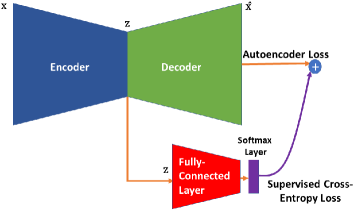
Figure 2: Schematic of a single layer Supervised Autoencoder Neural Network (SAE-NN)

2.2 Deep Supervised Autoencoder Classification Neural Networks (DSAE-NNs)

The overall goal is to learn a function that predicts the class labels in one-hot encoded form $\textbf{y}_{i}\in\mathbb{R}^{m}$ from inputs $\textbf{x}_{i}\in\mathbb{R}^{d_{x}}$. The operation performed by the encoder for a single hidden layer between the input variables to the latent variables $\mathbf{z}_{i}\in\mathbb{R}^{d_{z}}$ can be mathematically described as follows:

$$\textbf{z}_{i}=f_{e}(\textbf{W}_{e}\textbf{x}_{i}+\textbf{b}_{e})$$ (4)

The latent variables are used both to predict the class labels and to reconstruct back the inputs x as follows:

$$\hat{\textbf{x}_{i}}=f_{d}(\textbf{W}_{d}\textbf{z}_{i}+\textbf{b}_{d})$$ (5)

$$\hat{\textbf{y}_{i}}=f_{c}(\textbf{W}_{c}\textbf{z}_{i}+\textbf{b}_{c})$$ (6)

where $f_{c}$ is a non-linear activation function applied for the output layer. $\textbf{W}_{c}\in\mathbb{R}^{m\times d_{z}}$ and $\textbf{b}_{c}\in\mathbb{R}^{m}$ are output weight matrix and bias vector respectively. The training of an Deep Supervised Autoencoder Neural Network (DSAE-NN) model, schematically shown in Figure 2, is based on the minimization of a weighted sum of the reconstruction loss function and the supervised classification loss corresponding to the first and second terms in (Equation (7)) respectively. The reconstruction loss function in Equation (7) is ensuring that the estimated latent variables are able to capture the variance in the input data while the classification loss is ensuring that only those non-linear latent variables are extracted that are correlated with output classes. Mean squared error function is used as a reconstruction loss and softmax cross-entropy as the classification loss.

$$l_{DSAE} =\lambda_{1}\sum_{s=1}^{N}L_{r}^{s}(\textbf{x}_{s},\textbf{W}_{d}\textbf{W}_{e}\textbf{x}_{s})+\sum_{s=1}^{N}L_{p}^{s}(\textbf{W}_{c}\textbf{W}_{e}\textbf{x}_{s},\textbf{y}_{s})$$

$$=\frac{\lambda_{1}}{N}||\textbf{x}_{s}-\hat{\textbf{x}}_{s}||_{2}^{2}+\frac{1}{N}\sum_{s=1}^{N}\sum_{c=1}^{m}-y_{s,c}log(p_{s,c})$$

$$=\frac{1}{N}\bigg{[}\lambda_{1}||\textbf{x}_{s}-\hat{\textbf{x}}_{s}||_{2}^{2}+\sum_{s=1}^{N}\sum_{c=1}^{m}-y_{s,c}log(p_{s,c})\bigg{]}$$ (7)

$$p_{s,c} =\frac{e^{(\hat{y_{s,c}})}}{\sum_{c=1}^{m}e^{(\hat{y_{s,c}})}}$$ (8)

where $\lambda_{1}$ is the weight for the reconstruction loss $L_{r}$, $m$ is the number of classes, $y_{s,c}$ is a binary indicator (0 or 1) equal to 1 if the class label $c$ is the correct one for observation $s$ and 0 otherwise, $\hat{y_{s,c}}$ is the non-normalized log probabilities and $p_{s,c}$ is the predicted probability for a sample $s$ of class $c$. Moreover, to avoid over-fitting, a regularization term is added to the objective function in Equation 7. Hence, the objective function for Deep Supervised Autoencoder NNs used for Fault Detection (number of classes $m=2$, normal or faulty) is as follows:

$$\min_{\textbf{W}}l_{DSAE}=\min~{}~{}\frac{1}{N}\bigg{[}\lambda_{1}||\textbf{x}_{s}-\hat{\textbf{x}}_{s}||_{2}^{2}+\lambda_{2}\sum_{s=1}^{N}\sum_{c=1}^{m}-y_{s,c}log(p_{s,c})+\lambda_{3}\sum_{L}\sum_{k}\sum_{j}\textbf{W}_{{kj}}^{2[L]}\bigg{]}$$ (9)

where $\textbf{W}_{kj}^{[L]}$ are the weight matrices for each layer $L$ in the network (L = 1 in this example) and the weights on the individual objective functions $\lambda_{1},\lambda_{2},\lambda_{3}$ are chosen using validation data.

2.3 Dynamic Deep Supervised Autoencoder Classification Neural Networks (DDSAE-NNs)

The static DSAE-NN presented above assumes that the sampled data are independent to each other, and hence, temporal correlations are ignored. To account for the correlations in time between the data samples, a Dynamic Deep Supervised Autoencoders (DDSAE) model has been proposed by using a dynamic extension matrix. Accordingly, the original DSAE-NN model can be extended to take into account auto-correlations in time correlated data by augmenting each sample vector with the previous $l$ observations and stacking the data matrix with the resulting vectors, each corresponding to different time intervals.

The dynamic augmentation of the input data matrix $\textbf{X}_{D}$ by stacking previous $l$ observations to input data matrix X is as follows:

$$\textbf{X}_{D}=\big{[}\textbf{x}_{l+1}^{D}~{}\textbf{x}_{l+2}^{D}~{}\textbf{x}_{l+3}^{D}\ldots\textbf{x}_{N}^{D}\big{]}^{T}\in\mathbb{R}^{(N-l)\times((l+1)d_{x})}$$ (10)

where $\textbf{x}_{n}^{D}=[\textbf{x}_{n}~{}\textbf{x}_{n-1}~{}\textbf{x}_{n-2}\ldots\textbf{x}_{1}]$, where $\textbf{x}_{n}$ is a $\mathbb{R}^{d_{x}}$ dimensional vector of all the input feature vectors/ variables. The different time window length is chosen to build DDSAE models, in which the best classification performance is the final time window length. The following objective function ( Equation 11) is minimized with training data $\textbf{X}_{D}^{N-l+1}=\{\textbf{x}\}_{i=1}^{N-l+1},\textbf{y}_{D}=\{y\}_{i=1}^{N-l+1}$, where $N-l+1$ is the total number of samples:

$$\min_{\textbf{W}}l_{DDSAE}=\min~{}~{}\frac{1}{(N-l+1)}\bigg{[}\lambda_{1}||\textbf{x}^{D}_{s}-\hat{\textbf{x}}^{D}_{s}||_{2}^{2}+\lambda_{2}\sum_{s=1}^{N-l+1}\sum_{c=1}^{m}-y_{s,c}log(p_{s,c})+\lambda_{3}\sum_{L}\sum_{k}\sum_{j}\textbf{W}^{2[L]}_{{kj}}\bigg{]}$$ (11)

Note that the number of samples for the augmented dynamic matrix for the training data decreases as compared to the static DSAE case.

2.4 Layer-wise Relevance Propagation (LRP)

Layer-wise Relevance Propagation (LRP) was introduced by Bach et al., (2015)[4] to assess the relevance of each input variable or features with respect to outputs using a trained NN. It is based on a layer-wise relevance conservation principle where each relevance $[R_{c}(x_{i};f_{c})]_{j},~{}~{}i=1,2,...,n$, where $n$ is the number of input variables/ feature vectors ($x_{i},~{}~{}i=1,2,...,n$) for a $j^{th}$ sample where $j=1,2,...,N$, where $N$ is the total number of samples in the training dataset, is calculated by propagating the output scores for a particular task $c$ towards the input layer of the network. Previously, it has been used in the area of health-care for attributing a relevance value to each pixel of an image to explain the relevance in a image classification task using DNNs [45], to explain the predictions of a NN in the area of sentiment analysis [3], to identify the audio source in reverberant environments when multiple sources are active [30], and to identify EEG patterns that explain decisions in brain-computer interfaces [39]. In process systems engineering LRP has been recently applied by the authors for the first time for FDD problems. The method was used for identifying relevant input variables and pruning irrelevant input variables (input nodes) with respect to a specific classification task for both Multilayer Perceptron (MLP) NN and Long-Short Term Memory (LSTM) NN by Agarwal and Budman, (2019) [1, 2].

To compute the relevance of each input variable $x_{i},i=1,2,...,n$ for the DSAE-NNs and DDSAE-NNs models (used in this work), are trained for both fault detection and fault classification using the training dataset $\mbox{\Large$\chi$}:\{\textbf{X}^{l},\textbf{y}^{l}\}$ and $\mbox{\Large$\chi$}_{D}:\{\textbf{X}_{D}^{l},\textbf{y}_{D}^{l}\}$ ($\mbox{\Large$\chi$}_{D}$: dynamic version of $\chi$ ) respectively. Subsequently, the score value $f_{c}$ of the corresponding class for the $j^{th}$ sample is back-propagated through the network towards the input. Depending on the nature of the connection between layers and neurons, a layer-by-layer relevance score is computed for each intermediate lower-layer neuron. Different LRP rules have been proposed for attributing relevance for the input variables. In this work, we use the $\epsilon$ epsilon rule[4] for computing relevances that are given as follows:

$$R_{l\leftarrow u}=\sum_{u}\frac{x_{l}w_{lu}}{\sum_{j}x_{l}w_{lu}+\epsilon}R_{u}$$ (12)

where $\epsilon$ is used to prevent numerical instability when $z_{u}$ is close to zero and $w_{ul}$ are the weights connecting lower layer neurons $l$ and upper-layer neurons $u$. As $\epsilon$ becomes larger, only the most salient explanation factors survive the absorption. This typically leads to explanations that are sparser in terms of input features and less noisy [28]. Relevances $\textbf{R}_{c}(\textbf{x};\textbf{f}_{c})_{j}=[R_{c_{1}}(x_{1};f_{c}),R_{c_{2}}(x_{2};f_{c}),...,R_{c_{n}}(x_{n};f_{c})]_{j}\in\mathbb{R}^{n},~{}i=1,2,..,n$ for each input feature $x_{i}$ are calculated for the $j^{th}$ sample with respect to a classification task $c$ in the training dataset $\chi$ or $\mbox{\Large$\chi$}_{D}$. Since the goal is to prune the irrelevant input features DNNs based on estimated relevance scores using LRP, it is important to average the relevance scores over all the correctly classified samples in the training dataset. Therefore, the final input relevances with respect to the overall classification task $c$ can be calculated as follows:

$$\textbf{R}_{c}=\frac{1}{N_{c}}\sum_{j=1}^{N_{c}}\textbf{R}_{c}(\textbf{x};\textbf{f}_{c})_{j}$$ (13)

where $N_{c}$ is the number of correctly classified samples in the training dataset. Furthermore, the least relevant input features are pruned based on the average relevance scores for all input variables calculated with Equation 13. In practise a threshold of $\lambda\times\max(\textbf{R}_{c})$ is chosen to prune the irrelevant variables where $\lambda$ is an hyper-parameter that is determined by using the validation dataset (heuristically $\lambda$ is chosen as 0.01 as the starting value). Relevance of input variables below the threshold are removed from the dataset and the network is re-trained until the same or higher validation accuracy is achieved. It is to be noted that the DNN has to be re-trained with the set of remaining input variables after pruning and the testing accuracy increases with successive iterations as shown later in Section 4. For the dynamic augmented input matrix $\mbox{\Large$\chi$}_{D}$ shown in Equation 10, the final input relevances (combining effects of individual lagged variables) with respect to the overall classification task $c$ is:

$$\textbf{R}_{c}=\frac{1}{N_{c}}\sum_{j=1}^{N_{c}}\sum_{i=1}^{l+1}|R_{c_{i}}(x_{i};f_{c})|_{j}$$ (14)

where $l$ is the number of time lag window included in the dataset $\textbf{X}^{l}_{D}$.

3 Fault Detection and Diagnosis Methodology based on DSAE-NNs and DDSAE-NNs

Both the Deep Supervised Autoencoder NN (DSAE-NN)and Dynamic Deep Supervised Autoencoder NN (DDSAE-NN) are used for FDD and are the basis for the explainable-pruning based methodology presented in the previous section. The proposed fault detection algorithm is first used to extract deep features to detect if the process is operating in a normal or faulty region. Then, a fault diagnosis algorithm is applied in case the sample indicates faulty operation to identify the particular fault and possible root-cause of the occurring fault in the process using an DDSAE-NN. Since the latter is iteratively trained by using the LRP based pruning procedure that provides explainability of input variables the resulting DDSAE-NN model will be referred to as xDDSAE-NN.

3.1 Fault Detection Methodology

First, a DSAE-NN is trained using the training data ($\textbf{X}^{l},\textbf{y}^{l}$). The fault detection process is formulated as a binary classification problem. Often, this binary classification task for Fault Detection is susceptible to a ‘class imbalance problem’ because of the unequal distribution of classes in the training dataset. For example, the number of training samples for the normal operating region may be far less than the samples for abnormal operating region or vice-versa. To address this class imbalance problem an extra weight $\delta$ is introduced in the loss functions in Equation 15 and Equation 16 is as follows:

$$\min_{\textbf{W}}l_{DSAE}=\min~{}~{}\frac{1}{N}\bigg{[}\lambda_{1}\sum_{i=1}^{N}||\textbf{x}_{s}-\hat{\textbf{x}}_{s}||_{2}^{2}-\lambda_{2}\sum_{s=1}^{N}\big{(}\delta y_{s,1}\log(p_{s,1})+y_{s,2}\log(p_{s,2})\big{)}+\lambda_{3}\sum_{L}\sum_{k}\sum_{j}\textbf{W}_{kj}^{2[L]}\bigg{]}$$ (15)

$$\min_{\textbf{W}}l_{DDSAE}=\min~{}~{}\frac{1}{N}\bigg{[}\lambda_{1}\sum_{i=1}^{N}||\textbf{x}^{D}_{s}-\hat{\textbf{x}}^{D}_{s}||_{2}^{2}-\lambda_{2}\sum_{s=1}^{N}\big{(}\delta y_{s,1}\log(p_{s,1})+y_{s,2}\log(p_{s,2})\big{)}+\lambda_{3}\sum_{L}\sum_{k}\sum_{j}\textbf{W}_{{kj}}^{2[L]}\bigg{]}$$ (16)

For example, if there are more data samples of faulty operation than samples for normal operation higher weights would be assigned to the samples belonging to the normal operating region class. The value of $\delta$ dictates a trade-off between false positives and true negatives and is considered as an additional hyper-parameter to the model that is ultimately chosen using the validation data-set. Initially the DSAE-NN is trained on the training dataset ${\textbf{X}^{l},\textbf{y}^{l}}$ using all the input-variables. The best performing model is chosen using a validation dataset $\textbf{X}^{v},\textbf{y}^{v}$. Then, the LRP is implemented to explain the predictions of the chosen DSAE-NN with a set of hyper-parameters by computing the relevance of each input variable. The irrelevant input feature vectors are discarded based on a threshold as described in Section 2.4. Subsequently, the eXplainable DSAE (xDSAE) neural network is re-trained using the reduced training dataset $\{\textbf{X}^{l},\textbf{y}^{l}\}\rightarrow\{\textbf{X}^{l}_{r},\textbf{y}^{l}_{r}\}$ at each iteration. The premise for reducing the dimensionality of the input data by discarding less relevant inputs is that the information content can often be represented by a lower dimensional space, implying that only a few fundamental variables are sufficient to account for the variation in the data that are most informative about the identification of faults and normal regions. Once all the relevant input variables that are significant to the classification task are chosen, an eXplainable DDSAE-NN (xDDSAE-NN) is trained with the remaining inputs and the reduced training data matrix $\textbf{X}^{l}_{r}$ is augmented with the lagged variables of the remaining input variables $\textbf{X}^{l~{}D}_{r}$. The process of discarding input feature vectors is iterative and xDDSAE-NN is iteratively retrained using the validation dataset. This approach has multiple advantages over other reported methods used for fault detection as follows:

1. Improvement in test classification accuracy.

2. Identification of an eXplainable empirical model

3. Synthesis of a smaller network with fewer parameters

3.2 Fault Diagnosis Methodology

After detecting that the process has deviated from the normal operation and a fault has occurred, it is desired to diagnose the type of fault. For fault diagnosis, a similar methodology to the one used for fault detection is applied for the classification of the type of fault. First, the static DSAE is used to extract deep features and predict the type of fault in a process plant. For this task one-hot encoded outputs are utilized as the labels for training the model. Initially, the DSAE-NN is trained on the training dataset ${\textbf{X}^{l},\textbf{y}^{l}}$ using all the input-variables. The best performing model is chosen using a validation $\textbf{X}^{v},\textbf{y}^{v}$. LRP is subsequently implemented to explain the predictions of the selected DSAE-NN by computing the relevance of each input variable. The irrelevant features are removed by comparing the relevances to a threshold. Then an xDSAE NN is trained using the reduced training dataset $\textbf{X}^{l}_{r},\textbf{y}^{l}_{r}$ by successive iterations of pruning of irrelevant inputs and model re-training until the relevance of all the remaining input variables are above the threshold. Since data collected from chemical processes have strong dynamic/temporal correlations, the input data matrix X is augmented with observations at $l$ previous time steps for each input feature dimension (refer Equation 10) and a DDSAE-NN is trained. The iterative procedure of discarding input variables from the reduced dynamic matrix $\textbf{X}^{l~{}D}_{r}$ is implemented and pruning and re-training is applied as long as validation accuracy continue to increase after discarding features. The decision of adding lagged variables only to the remaining input variables of the final iteration of xDSAE model is justified by the fact that the input variables that were eliminated do not have an instantaneous effect of $x_{k}$ on fault detection. Then, since the pruned input variables at current time are auto-correlated in time to previous values ($x_{k}\propto f(\textbf{x}_{k-1},\textbf{x}_{k-2},..,\textbf{x}_{k-n})$), if current values are not correlated to the model outputs then their corresponding previous values (lagged variables) are also not correlated to these outputs.

3.3 Proposed Methodology for FDD

The proposed methodology for FDD is schematically described in Figure 3 and it is summarized by the following steps.

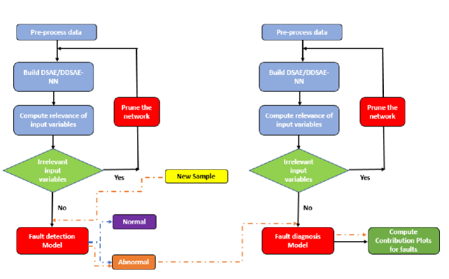
Figure 3: Flowchart for fault detection and diagnosis based on explainable DNN

1. Pre-process the input data. $\textbf{X}_{\text{raw}}\rightarrow\textbf{X}^{l}$.

2. Build a DSAE-NN that maps the input vectors into the latent feature space by using a DSAE model structure. The goal is to extract discriminative features that capture the latent manifold in the input data that are most correlated with the output classes. The parameters are optimized using a combination of the reconstruction error, $L_{2}$ regularization error and binary softmax cross-entropy error of the input data (refer Equation 15).

3. Select the best performing model architecture (number of layers and nodes) along with the set of hyper-parameters that include learning rate, batch size, and all other weighting ($\lambda_{1},\lambda_{2},\lambda_{3}$ and $\delta$) parameters using the validation dataset. ($\textbf{X}^{v},\textbf{y}^{v}$).

4. Evaluate the classification accuracy using the chosen trained DSAE model in Step 3 for testing dataset  ($\textbf{X}^{t},\textbf{y}^{t}$). If the model in testing is satisfactory, the model will be used for further analysis; if unsatisfactory, return to Step 3 to redesign the DSAE-NN model.

5. Compute input relevances using the LRP method on the test dataset and discard irrelevant input features from the dataset $\textbf{X}^{l},\textbf{X}^{v}$ and $\textbf{X}^{t}$.

6. Repeat steps 3,4 and 5 until relevances of all input variables are above the threshold and no improvement over the validation accuracy is achieved for xDSAE NN.

7. Build xDDSAE model using the reduced input dataset $\textbf{X}^{l}_{r}$ computed in Step 6 along with augmenting $l$ lagged variables.

8. Select the best performing model architecture (number of layers and nodes) using the validation dataset ($\textbf{X}^{v}_{r},\textbf{y}^{v}_{r}$).

9. Repeat steps 3,4 and 5 until relevances of all input variables are above the threshold and no improvement of the validation accuracy is achieved.

10. For online process monitoring: When a new data vector $\textbf{X}_{new}$ becomes available, import it into the model after normalizing to determine whether the current state of the process is in normal or abnormal operating region and to determine the type of fault that is responsible for the deviation.

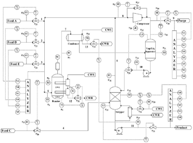
Figure 4: Schematic: Tennessee Eastman plant process (Downs and Vogel, 1993)

Table 1: Measured and manipulated variables (from Downs and Vogel, 1993)

Variable Name	Variable Number	Units	Variable Name	Variable Number	Units
A feed (stream 1)	XMEAS (1)	kscmh	Reactor cooling water outlet temperature	XMEAS (21)	∘ C
D feed (stream 2)	XMEAS (2)	kg h-1	Separator cooling water outlet temperature	XMEAS (22)	∘C
E feed (stream 3)	XMEAS (3)	kg h-1	Feed %A	XMEAS(23)	mol%
A and C feed (stream 4)	XMEAS (4)	kscmh	Feed %B	XMEAS(24)	mol%
Recycle flow (stream 8)	XMEAS (5)	kscmh	Feed %C	XMEAS(25)	mol%
Reactor feed rate (stream 6)	XMEAS (6)	kscmh	Feed %D	XMEAS(26)	mol%
Reactor pressure	XMEAS (7)	kPa guage	Feed %E	XMEAS(27)	mol%
Reactor level	XMEAS (8)	%	Feed %F	XMEAS(28)	mol%
Reactor temperature	XMEAS (9)	∘C	Purge %A	XMEAS(29)	mol%
Purge rate (stream 9)	XMEAS (10)	kscmh	Purge %B	XMEAS(30)	mol%
Product separator temperature	XMEAS (11)	∘C	Purge %C	XMEAS(31)	mol%
Product separator level	XMEAS (12)	%	Purge %D	XMEAS(32)	mol%
Product separator pressure	XMEAS (13)	kPa guage	Purge %E	XMEAS(33)	mol%
Product separator underflow (stream 10)	XMEAS (14)	m3 h-1	Purge %F	XMEAS(34)	mol%
Stripper level	XMEAS (15)	%	Purge %G	XMEAS(35)	mol%
Stripper pressure	XMEAS (16)	kPa guage	Purge %H	XMEAS(36)	mol%
Stripper underflow (stream 11)	XMEAS (17)	m3 h-1	Product %D	XMEAS(37)	mol%
Stripper temperature	XMEAS (18)	∘C	Product %E	XMEAS(38)	mol%
Stripper steam flow	XMEAS (19)	kg h-1	Product %F	XMEAS(39)	mol%
Compressor Work	XMEAS (20)	kW	Product %G	XMEAS(40)	mol%
D Feed Flow	XMV (1)	kg h-1	Product %H	XMEAS(41)	mol%
E Feed Flow	XMV (2)	kg h-1	A Feed Flow	XMV (3)	kscmh
A + C Feed Flow	XMV (4)	kscmh	Compressor Recycle Valve	XMV(5)	%
Purge Valve	XMV (6)	%	Separator pot liquid flow	XMV (7)	m3h-1
Stripper liquid product flow	XMV (8)	m3h-1	Stripper Steam Valve	XMV (9)	%
Reactor cooling water flow	XMV (10)	m3h-1	Condenser cooling water flow	XMV (11)	m3h-1

Table 2: Process Faults for classification in TE Process

Fault	Description	Type
IDV(1)	A/C feed ratio, B composition constant (stream 4)	step
IDV(2)	B composition, A/C ratio constant (stream 4)	step
IDV(3)	D Feed Temperature	step
IDV(4)	Reactor cooling water inlet temperature	step
IDV(5)	Condenser cooling water inlet temperature (stream 2)	step
IDV(6)	A feed loss (stream 1)	step
IDV(7)	C header pressure loss reduced availability (stream 4)	step
IDV(8)	A, B, C feed composition (stream 4)	random variation
IDV(9)	D Feed Temperature	random variation
IDV(10)	C feed temperature (stream 4)	random variation
IDV(11)	Reactor cooling water inlet temperature	random variation
IDV(12)	Condenser cooling water inlet temperature	random variation
IDV(13)	Reaction kinetics	slow drift
IDV(14)	Reactor cooling water	valve sticking
IDV(15)	Condenser Cooling Water Valve	stiction
IDV(16)	Deviations of heat transfer within stripper	random variation
IDV(17)	Deviations of heat transfer within reactor	random variation
IDV(18)	Deviations of heat transfer within condenser	random variation
IDV(19)	Recycle valve of compressor, underflow stripper and steam valve stripper	stiction
IDV(20)	unknown	random variation

4 Case Study: Tennessee Eastman Process

In this section the proposed methodology is implemented for FDD and the performance is compared with different approaches in the literature on the benchmark Tennessee Eastman Process (TEP). The Tennessee Eastman plant has been used widely for testing several process monitoring and fault detection algorithms [9, 24, 31, 44, 33, 5, 22, 23]. The TEP involves different unit operations including a vapor-liquid separator, a reactor, stripper a recycle compressor and a condenser. Four gaseous reactants (A, B, C and D) forms two liquid products streams (G and H) and a by-product (F). A schematic of the Tennessee Eastman Process is illustrated in Figure 4. Downs and Vogel (1993)[10] reported the original simulator for this process and has been widely used as a benchmark process for control and monitoring studies (simulator available at http://depts.washington.edu/control/LARRY/TE/download.html). The process simulator involves a total of $52$ measured variables including $22$ process (output) variables, $12$ manipulated variables and $19$ composition measurements. A complete list of output measurements and manipulated variables are presented in Table 1. Additional details about the process model can be found in the original paper [10] and descriptions of the different control schemes that have been applied to the simulator can be found in [33] and its revised version [5]. Several data-driven statistical process monitoring approaches have been reported for the detection and diagnosis of disturbances in the Tennessee Eastman simulation. There are $20$ different process disturbances (fault types) in the industrial simulator (shown in Table 2) though only $17$ were used in this work to be consistent with other methods in the literature. Each of these methods has shown different levels of success in detecting and diagnosing the faults considered in the simulations (Table 1). Several statistical studies have reported faults 3, 9 and 15 as unobservable or difficult to diagnose due to the close similarity in the responses of the noisy measurements used to detect these faults [24, 35, 9, 11] and therefore these 3 faults were not considered in the current study.

The training data consists of $500$ samples of normal data and $480$ samples for each fault. The testing dataset has $960$ samples for both faulty and normal operation data. For the faulty testing dataset, the fault is introduced at $160$ time-sample. A part of the training data $\{\textbf{X}^{l},\textbf{y}^{l}\}$ is used as the validation dataset $\{\textbf{X}^{v},\textbf{y}^{v}\}$ for tuning the hyper-parameters (learning rate, weights: $\lambda,\lambda_{1},~{}\lambda_{2},~{}\lambda_{3}$ and $\delta$, number of epochs,layers an nodes in each layer) for both DSAE/ xDSAE and DDSAE/ xDDSAE DNNs for all iterations. The network architecture and test accuracies for fault detection and fault classification are presented in Table 3 and 4 respectively. After applying the LRP procedure to the static fault detection model, it is found that only 24 out of 52 variables are the most important for obtaining the highest testing accuracy for detecting the correct state of the process plant. After every iteration of the input pruning-relevance (LRP) based procedure it is shown in Table 3 that the removal of irrelevant input variables results in successive improvement of fault class separability. To account for the dynamic information after identifying the 24 most relevant process variables, the reduced input data matrix $\{\textbf{X}^{l}_{r}\}$ is stacked with lagged time stamps and an DDSAE NN model is retrained. The best fault detection test accuracy of $96.43\%$ is achieved by stacking two previous time-stamp process values. The fault detection rates for all the faults are shown in Table 5. These results are compared in the same Table 5 with several methods as follows: PCA [26], DPCA[26], ICA[16], Convolutional NN (CNN) [37], Deep Stacked Network (DSN) [6], Stacked Autoencoder (SAE) [6], Generative Adversarial Network (GAN) [38] and One-Class SVM (OCSVM) [38]. It can been seen from Table 5 that the proposed method outperformed the linear multivariate methods and other DL based methods for most fault modes. For example, for PCA with 15 principal components, the average fault detection rates are 61.77% and 74.72% using $T^{2}$ and $Q$ statistic respectively. Since the principal components extracted using PCA captures static correlations between variables, DPCA (Dynamic PCA) is used to account for temporal correlations (both auto-correlations and cross-correlations) in the data. Since DPCA is only an input data compression technique, it must be combined with a classification model for the purpose of fault detection. Accordingly, the output features from the DPCA model are fed into an SVM model that is used for final classification. The effect of increasing the number of lagged variables in the dataset is also investigated following the hypothesis that increasing the time horizon will enhance classification accuracy. It can be seen in Table 3 that the increasing number of lags and simultaneous pruning improves the classification accuracy. The average detection rate obtained was 72.35%. ICA [16] based monitoring scheme was found to perform better than both PCA and DPCA based methods with an averaged accuracy of approximately 90%. In addition to the comparison to linear methods, the proposed methodology was also compared with different DNN architectures such as CNN[6], DSN [6], SAE-NN (results reported in Chadha and Schwung,2017) and GAN[38], OCSVM (results reported in Spyridon and Boutalis,2018) reported previously. It can be seen that the proposed method also outperforms these DNN based methodologies. Also, the false alarm rate (FAR) i.e. normal samples miss-classified as faulty is $1.46\%$ which is the lowest as compared to all the other methods.

Table 3: Network Architecture and iterations for fault detection methodology

Iteration	Network Type DSAE/ DDSAE	Architecture	Averaged Test Classification Accuracy (FDR)
1	DSAE	$52-5-10^{*}-10-5-52$	91.55%
2	xDSAE	$30-5-10^{*}-10-5-30$	93%
3	xDSAE	$24-7-6^{*}-6-7-30$	93.23%
1	DDSAE (lag1)	$48-4-6^{*}-6-4-48$	93.96%
2	xDDSAE (lag1)	$46-5-7^{*}-7-5-46$	95.52%
3	xDDSAE (lag1)	$41-5-10^{*}-10-5-41$	95.63%
4	xDDSAE (lag1)	$40-5-10^{*}-10-2-40$	95.85%
1	DDSAE (lag2)	$72-4-10^{*}-10-4-72$	93.5%
2	xDDSAE (lag2)	$70-2-10^{*}-10-2-70$	93.53%
3	xDDSAE (lag2)	$54-4-10^{*}-10-4-54$	95.44%
4	xDDSAE (lag2)	$50-6-12^{*}-12-6-50$	96.43%

• A dense layer is present where the number of input nodes are shown with an asterisk and the number of output nodes are 2 (equal to the number of classes).

Figure 5: Final Iteration: Averaged Relative Relevance Plot for Fault Detection (DDSAE Model with 2 lagged input variables as $\textbf{X}^{l}$)

Table 4: Network Architecture and iterations for fault diagnosis methodology

Iteration	Network Type DSAE/ DDSAE	Architecture	Averaged Test Classification Accuracy (FDR)
1	DSAE	$52-25-20-20^{*}-20-20-25-52$	81.90%
2	xDSAE	$45-10-10-20^{*}-20-10-10-45$	82.60%
3	xDSAE	$33-21-20-20^{*}-20-20-21-33$	83.15%
1	DDSAE (5 lags)	$198-14-10-30^{*}-30-10-14-198$	83.41%
2	xDDSAE (5 lags)	$159-24-10-30^{*}-30-10-24-159$	85.14%
3	xDDSAE (5 lags)	$155-24-8-30^{*}-30-8-24-155$	85.87%
4	xDDSAE (5 lags)	$140-30-20-17^{*}-17-20-30-140$	86.91%
1	DDSAE (10 lags)	$363-14-20-30^{*}-30-20-14-363$	83.08%
2	xDDSAE (10 lags)	$317-18-15-30^{*}-30-15-18-317$	85.04%
3	xDDSAE (10 lags)	$293-24-18-30^{*}-30-18-24-293$	85.51%
4	xDDSAE (10 lags)	$259-28-18-30^{*}-30-18-28-259$	87.07%
5	xDDSAE (10 lags)	$244-34-20-30^{*}-30-20-34-244$	87.86%
6	xDDSAE (10 lags)	$235-38-21-30^{*}-30-21-38-235$	88.41%

• A dense layer is present where the number of input nodes are shown with an asterisk and the number of output nodes are 17 (equal to the number of classes).

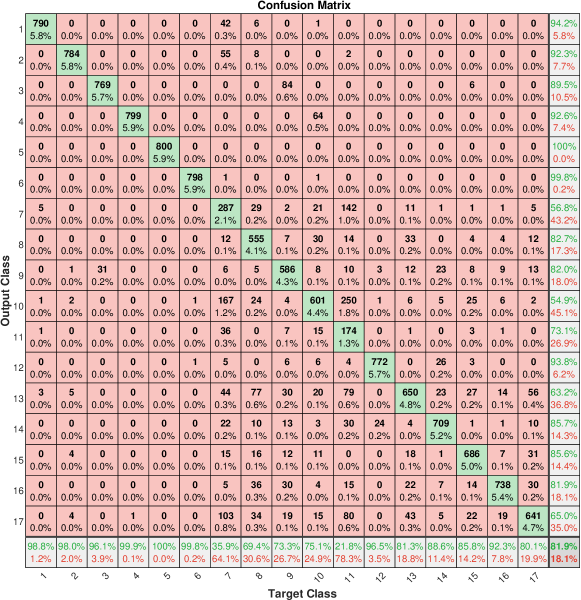
Figure 6: Confusion Matrix for Fault Classification (First Iteration: DSAE Model with 52 input variables)

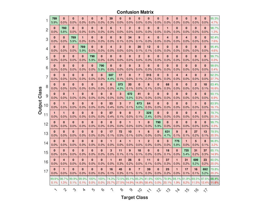
Figure 7: Confusion Matrix for Fault Classification (Final Iteration: DDSAE Model with 10 lagged input variables)

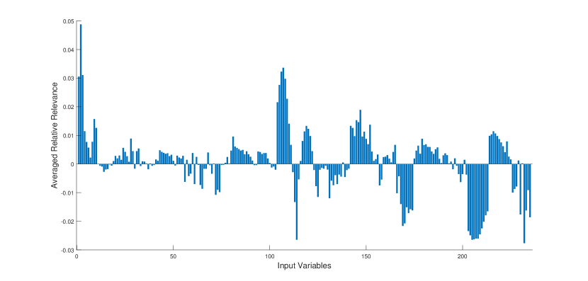
Figure 8: Final Iteration: Averaged Relative Relevance Plot for Fault Diagnosis (DDSAE Model with 10 lagged input variables as $\textbf{X}^{l}$)

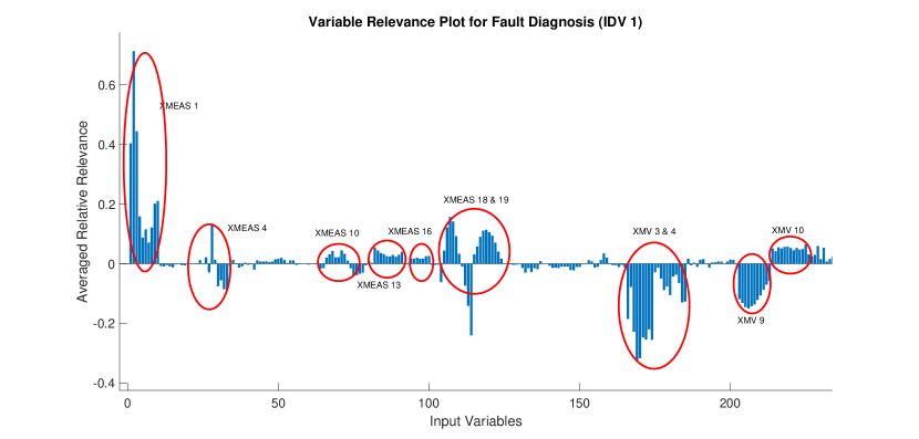
Figure 9: Input variable relevance plot for Fault Diagnosis (IDV 1)

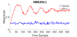
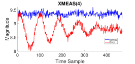
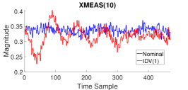
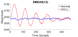
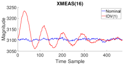
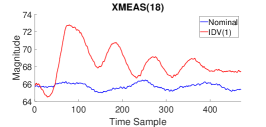
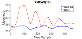
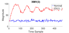
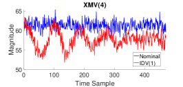
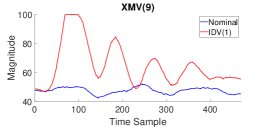
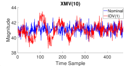
Figure 10: Relevant variables contributing to IDV(1) with nominal and abnormal profiles

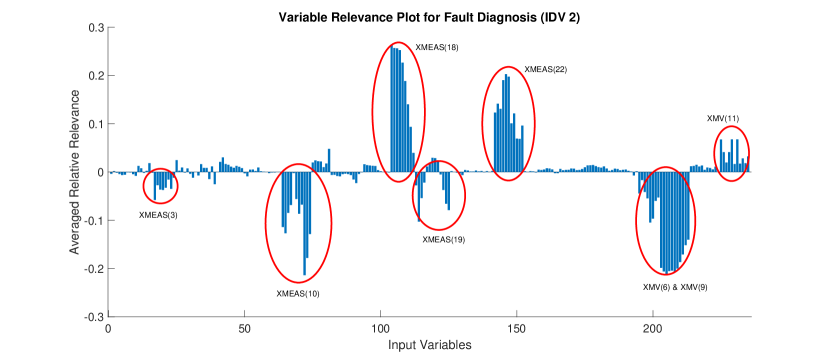
Figure 11: Input variable relevance plot for Fault Diagnosis (IDV 2)

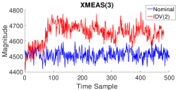
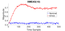
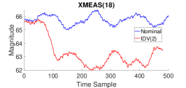
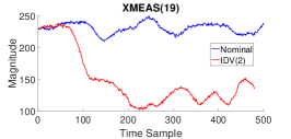
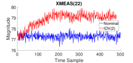
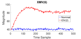
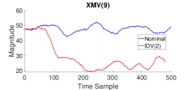
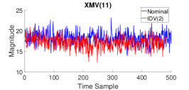
Figure 12: Relevant variables contributing to IDV(2) with nominal and abnormal profiles

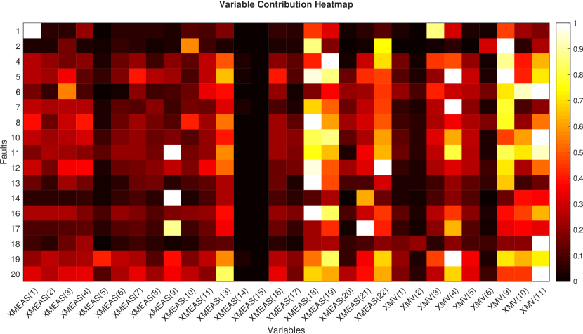
Figure 13: Variable Contribution Heatmap corresponding to all faults

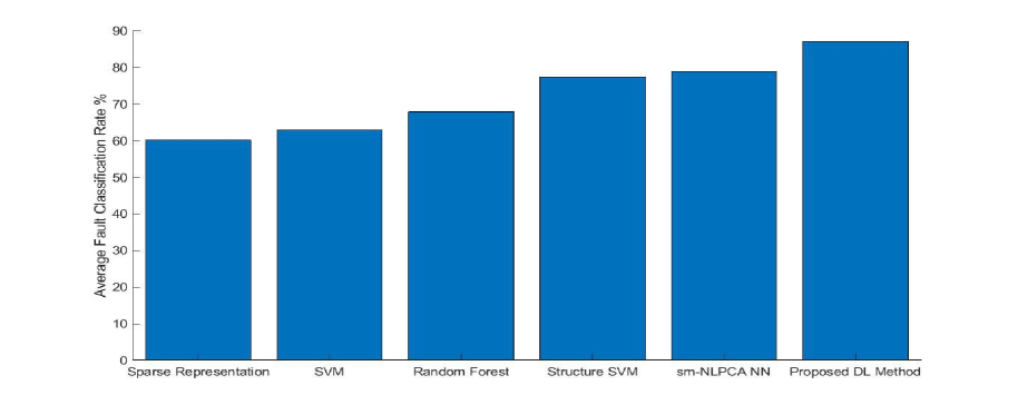
Figure 14: Comparison of Fault Classification rate with different methods

Table 5: Comparison of Fault Detection Rate with different methods with non-incipient faults only

Fault	PCA (15 comp.)		DPCA (22 comp.)	ICA (9 comp.)		DL (2017)	DL (2017)	DL (2018)	DL (2018)	DL (2019)	Proposed DL
	$T^{2}$	SPE	$T^{2}$	$I^{2}$	AO	SAE-NN	DSN	GAN	OCSVM	CNN	DDSAE
1	99.2%	99.8%	99%	100%	100%	77.6%	90.8%	99.62%	99.5%	91.39%	99.9%
2	98%	98.6%	98%	98%	98%	85%	89.6%	98.5%	98.5%	87.96%	98.2%
4	4.4%	96.2%	26%	61%	84%	56.6%	47.6%	56.25%	50.37%	99.73%	99.7%
5	22.5%	25.4%	36%	100%	100%	76%	31.6%	32.37%	30.5%	90.35%	100%
6	98.9%	100%	100%	100%	100%	82.8%	91.6%	100%	100%	91.5%	99.7%
7	91.5%	100%	100%	99%	100%	80.6%	91%	99.99%	99.62%	91.55%	99.9%
8	96.6%	97.6%	98%	97%	97%	83%	90.2%	97.87%	97.37%	82.95%	94%
10	33.4%	34.1%	55%	78%	82%	75.3%	63.2%	50.87%	53.25%	70.05%	89.1%
11	20.6%	64.4%	48%	52%	70	75.9%	54.2%	58%	54.75%	60.16%	87.7%
12	97.1%	97.5%	99%	99%	100%	83.3%	87.8%	98.75%	98.63%	85.56%	99.4%
13	94%	95.5%	94%	94%	95%	83.3%	85.5%	95%	94.87%	46.92%	95.6%
14	84.2%	100%	100%	100%	100%	77.8%	89%	100%	100 %	88.88%	100%
16	16.6%	24.5%	49%	71%	78%	78.3%	74.8%	34.37%	36.37%	66.84%	94%
17	74.1%	89.2%	82%	89%	94%	78%	83.3%	91.12%	87.25%	77.11%	97.7%
18	88.7%	89.9%	90%	90%	90%	83.3%	82.4%	90.37%	90.12%	82.74%	90.9%
19	0.4%	12.7%	3%	69%	80%	67.7%	52.4%	11.8%	3.75%	70.87%	89.9%
20	29.9%	45%	53%	87%	91%	77.1%	44.1%	58.37%	52.75%	72.88%	89.6%
Average	61.77%	74.72%	72.35%	87.29%	91.70%	77.7%	76.84%	74.04%	62.78%	85.47%	96.43%

For fault classification with the static DSAE-NN models it is observed that only 235 out of 363 input variables are the most relevant features for obtaining the highest testing accuracy in identifying the type of fault. Every iteration of the proposed methodology conducted for pruning of irrelevant input features increase the classification accuracy as shown in Table 4. After identifying the 33 most relevant process variables with the static DSAE-NN model, the reduced input data matrix $\{\textbf{X}^{l}_{r}\}$ is stacked with lagged time stamps $\{\textbf{X}^{l}_{r}\}\rightarrow\{\textbf{X}^{lD}_{r}\}$ and the network is retrained. The best test classification accuracy of $88.41\%$ is achieved by stacking ten previous time-stamp process values. The confusion matrices for the first iteration and the final iteration are shown in Figure 6 and 7 respectively. It can be seen that there is a significant improvement in the average test classification due to the implementation of proposed methodology. For example: there is an increase of $38\%$ in degree of separability in IDV(8) and $20\%$ increase in IDV(13).The averaged test accuracy for fault classification problem is compared with various non-linear classification algorithms such as Sparse representation, SVM, Random Forest, Structure SVM, AE based classification (sm-NLPCA) method. As shown in Figure 14 the proposed methodology outperforms other methods by a significant margin. The averaged relative importance of each relevant input feature $\textbf{R}_{c}$ (estimated using Equation 14) towards the classification task $c$ (fault classification) is shown in Figure 8. An important by-product of the proposed pruning methodology is that it can explain which input variables significantly deviate from their normal trajectories while the fault is occurring or to identify the root cause of the process fault. Towards that task, averaged input relevances’ values for the correctly classified samples for a specific process fault are computed using LRP. For example for Fault 1 (a step change in A/C Feed ratio) the average relative relevance plot for IDV(1) is shown in Figure 9. Then, using this plot which are the variables that will significantly deviate from their trajectories during normal operation following the occurrence of the fault. Figure 10 shows the evolution of the IDV(1) relevant input variables as a function of time. This figure corroborates that all the identified variables according to the average relevance analysis do significantly deviate from their nominal operation values during the occurrence of fault IDV(1). Similarly, an averaged relative relevance plot for IDV(2) is shown in Figure 11 and the input variables identified as significant to detect this fault are then plotted in Figure 12 as functions of time corroborating that the variables identified as significant in the plot 11 are significantly deviating following the fault from their trajectories during normal operation. Similar diagnostics can be run for all the other faults for the TEP problem.

Finally, for easier visualization, using these average relative relevances’ values for each fault a variable contribution heatmap is generated and shown in Figure 13 can be computed using Equation 14. In this heatmap the significance of different variables are color coded to identify the possible root-cause of different variables for each particular fault. For example for fault 1, variables 1 and 3 are shown as significant in the heatmap and it can be verified from Figure 9 that these same variables deviate the most during faulty operation from their trajectories during normal operation.

5 Conclusion

In this paper, an explainability based fault detection and classification methodology is proposed using both a deep supervised autoencoder (DSAE) and dynamic supervised autoencoder (DDSAE) for the extraction of features. A Layerwise Relevance Propagation (LRP) algorithm is used as the main tool for explaining the classification predictions for the deep neural networks. The explainability measure serves two major objectives: i) Pruning of irrelevant input variables and further improvement in the test classification accuracy and ii) Identification of possible root cause of different faults occurring in the process. The fault detection and classification performance of the proposed DSAE/xDSAE and DDSAE/xDSSAE DNN models together is tested on the TE benchmark process. The proposed methodology outperforms both multivariate linear methods and other DL based methods reported in the literature on the same standard data.

Although this study make use of the powerful feature extraction capability of deep learning neural network models and XAI (eXplainable AI) their use in industrial processes must face practical challenges such as availability of data for training and a longer development time for off-line model calibration because of the sequence of pruning and re-training steps.

6 Acknowledgement

This work is the result of the research project supported by MITACS grant IT10393 through MITACS-Accelerate Program.

References

- Agarwal and Budman [2019] Agarwal, P., Budman, H., 2019. Classification of profit-based operating regions for the tennessee eastman process using deep learning methods. IFAC-PapersOnLine 52, 556–561.
- Agarwal et al. [2019] Agarwal, P., Tamer, M., Sahraei, M.H., Budman, H., 2019. Deep learning for classification of profit-based operating regions in industrial processes. Industrial & Engineering Chemistry Research .
- Arras et al. [2017] Arras, L., Montavon, G., Müller, K.R., Samek, W., 2017. Explaining recurrent neural network predictions in sentiment analysis. arXiv preprint arXiv:1706.07206 .
- Bach et al. [2015] Bach, S., Binder, A., Montavon, G., Klauschen, F., Müller, K.R., Samek, W., 2015. On pixel-wise explanations for non-linear classifier decisions by layer-wise relevance propagation. PloS one 10, e0130140.
- Bathelt et al. [2015] Bathelt, A., Ricker, N.L., Jelali, M., 2015. Revision of the tennessee eastman process model. IFAC-PapersOnLine 48, 309–314.
- Chadha and Schwung [2017] Chadha, G.S., Schwung, A., 2017. Comparison of deep neural network architectures for fault detection in tennessee eastman process, in: 2017 22nd IEEE International Conference on Emerging Technologies and Factory Automation (ETFA), IEEE. pp. 1–8.
- Chen et al. [2015] Chen, Z., Li, C., Sanchez, R.V., 2015. Gearbox fault identification and classification with convolutional neural networks. Shock and Vibration 2015.
- Chiang et al. [2004] Chiang, L.H., Kotanchek, M.E., Kordon, A.K., 2004. Fault diagnosis based on fisher discriminant analysis and support vector machines. Computers & chemical engineering 28, 1389–1401.
- Chiang et al. [2000] Chiang, L.H., Russell, E.L., Braatz, R.D., 2000. Fault diagnosis in chemical processes using fisher discriminant analysis, discriminant partial least squares, and principal component analysis. Chemometrics and intelligent laboratory systems 50, 243–252.
- Downs and Vogel [1993] Downs, J.J., Vogel, E.F., 1993. A plant-wide industrial process control problem. Computers & chemical engineering 17, 245–255.
- Du and Du [2018] Du, Y., Du, D., 2018. Fault detection using empirical mode decomposition based pca and cusum with application to the tennessee eastman process. IFAC-PapersOnLine 51, 488–493.
- Gan et al. [2016] Gan, M., Wang, C., et al., 2016. Construction of hierarchical diagnosis network based on deep learning and its application in the fault pattern recognition of rolling element bearings. Mechanical Systems and Signal Processing 72, 92–104.
- Harmouche et al. [2014] Harmouche, J., Delpha, C., Diallo, D., 2014. Incipient fault detection and diagnosis based on kullback–leibler divergence using principal component analysis: Part i. Signal Processing 94, 278–287.
- He and He [2017] He, M., He, D., 2017. Deep learning based approach for bearing fault diagnosis. IEEE Transactions on Industry Applications 53, 3057–3065.
- Hoskins et al. [1991] Hoskins, J., Kaliyur, K., Himmelblau, D.M., 1991. Fault diagnosis in complex chemical plants using artificial neural networks. AIChE Journal 37, 137–141.
- Hsu et al. [2010] Hsu, C.C., Chen, M.C., Chen, L.S., 2010. A novel process monitoring approach with dynamic independent component analysis. Control Engineering Practice 18, 242–253.
- Janssens et al. [2016] Janssens, O., Slavkovikj, V., Vervisch, B., Stockman, K., Loccufier, M., Verstockt, S., Van de Walle, R., Van Hoecke, S., 2016. Convolutional neural network based fault detection for rotating machinery. Journal of Sound and Vibration 377, 331–345.
- Jia et al. [2016] Jia, F., Lei, Y., Lin, J., Zhou, X., Lu, N., 2016. Deep neural networks: A promising tool for fault characteristic mining and intelligent diagnosis of rotating machinery with massive data. Mechanical Systems and Signal Processing 72, 303–315.
- Jing et al. [2017] Jing, L., Zhao, M., Li, P., Xu, X., 2017. A convolutional neural network based feature learning and fault diagnosis method for the condition monitoring of gearbox. Measurement 111, 1–10.
- Kaistha and Upadhyaya [2001] Kaistha, N., Upadhyaya, B., 2001. Incipient fault detection and isolation in a pwr plant using principal component analysis, in: Proceedings of the 2001 American Control Conference.(Cat. No. 01CH37148), IEEE. pp. 2119–2120.
- Ku et al. [1995] Ku, W., Storer, R.H., Georgakis, C., 1995. Disturbance detection and isolation by dynamic principal component analysis. Chemometrics and intelligent laboratory systems 30, 179–196.
- Kulkarni et al. [2005] Kulkarni, A., Jayaraman, V.K., Kulkarni, B.D., 2005. Knowledge incorporated support vector machines to detect faults in tennessee eastman process. Computers & chemical engineering 29, 2128–2133.
- Larsson et al. [2001] Larsson, T., Hestetun, K., Hovland, E., Skogestad, S., 2001. Self-optimizing control of a large-scale plant: The tennessee eastman process. Industrial & engineering chemistry research 40, 4889–4901.
- Lau et al. [2013] Lau, C., Ghosh, K., Hussain, M.A., Hassan, C.C., 2013. Fault diagnosis of tennessee eastman process with multi-scale pca and anfis. Chemometrics and Intelligent Laboratory Systems 120, 1–14.
- Lundberg and Lee [2017] Lundberg, S., Lee, S.I., 2017. A unified approach to interpreting model predictions. arXiv preprint arXiv:1705.07874 .
- Lv et al. [2016] Lv, F., Wen, C., Bao, Z., Liu, M., 2016. Fault diagnosis based on deep learning, in: 2016 American Control Conference (ACC), IEEE. pp. 6851–6856.
- Mahadevan and Shah [2009] Mahadevan, S., Shah, S.L., 2009. Fault detection and diagnosis in process data using one-class support vector machines. Journal of process control 19, 1627–1639.
- Montavon et al. [2019] Montavon, G., Binder, A., Lapuschkin, S., Samek, W., Müller, K.R., 2019. Layer-wise relevance propagation: an overview. Explainable AI: interpreting, explaining and visualizing deep learning , 193–209.
- Odiowei and Cao [2009] Odiowei, P.E.P., Cao, Y., 2009. Nonlinear dynamic process monitoring using canonical variate analysis and kernel density estimations. IEEE Transactions on Industrial Informatics 6, 36–45.
- Perotin et al. [2019] Perotin, L., Serizel, R., Vincent, E., Guérin, A., 2019. Crnn-based multiple doa estimation using acoustic intensity features for ambisonics recordings. IEEE Journal of Selected Topics in Signal Processing 13, 22–33.
- Rato and Reis [2013] Rato, T.J., Reis, M.S., 2013. Fault detection in the tennessee eastman benchmark process using dynamic principal components analysis based on decorrelated residuals (dpca-dr). Chemometrics and Intelligent Laboratory Systems 125, 101–108.
- Ribeiro et al. [2016] Ribeiro, M.T., Singh, S., Guestrin, C., 2016. " why should i trust you?" explaining the predictions of any classifier, in: Proceedings of the 22nd ACM SIGKDD international conference on knowledge discovery and data mining, pp. 1135–1144.
- Ricker [1996] Ricker, N.L., 1996. Decentralized control of the tennessee eastman challenge process. Journal of Process Control 6, 205–221.
- Rios et al. [2020] Rios, A., Gala, V., Mckeever, S., et al., 2020. Explaining deep learning models for structured data using layer-wise relevance propagation. arXiv preprint arXiv:2011.13429 .
- Shams et al. [2010] Shams, M.B., Budman, H., Duever, T., 2010. Fault detection using cusum based techniques with application to the tennessee eastman process. IFAC Proceedings Volumes 43, 109–114.
- Shrikumar et al. [2017] Shrikumar, A., Greenside, P., Kundaje, A., 2017. Learning important features through propagating activation differences, in: International Conference on Machine Learning, PMLR. pp. 3145–3153.
- Singh Chadha et al. [2019] Singh Chadha, G., Krishnamoorthy, M., Schwung, A., 2019. Time series based fault detection in industrial processes using convolutional neural networks, in: IECON 2019 - 45th Annual Conference of the IEEE Industrial Electronics Society, pp. 173–178. doi:10.1109/IECON.2019.8926924.
- Spyridon and Boutalis [2018] Spyridon, P., Boutalis, Y.S., 2018. Generative adversarial networks for unsupervised fault detection, in: 2018 European Control Conference (ECC), IEEE. pp. 691–696.
- Sturm et al. [2016] Sturm, I., Lapuschkin, S., Samek, W., Müller, K.R., 2016. Interpretable deep neural networks for single-trial eeg classification. Journal of neuroscience methods 274, 141–145.
- Sun et al. [2016] Sun, W., Shao, S., Zhao, R., Yan, R., Zhang, X., Chen, X., 2016. A sparse auto-encoder-based deep neural network approach for induction motor faults classification. Measurement 89, 171–178.
- Wang et al. [2018] Wang, H.g., Li, X., Zhang, T., 2018. Generative adversarial network based novelty detection usingminimized reconstruction error. Frontiers of Information Technology & Electronic Engineering 19, 116–125.
- Wise et al. [1990] Wise, B.M., Ricker, N., Veltkamp, D., Kowalski, B.R., 1990. A theoretical basis for the use of principal component models for monitoring multivariate processes. Process control and quality 1, 41–51.
- Wu and Zhao [2018] Wu, H., Zhao, J., 2018. Deep convolutional neural network model based chemical process fault diagnosis. Computers & chemical engineering 115, 185–197.
- Xie and Bai [2015] Xie, D., Bai, L., 2015. A hierarchical deep neural network for fault diagnosis on tennessee-eastman process, in: 2015 IEEE 14th International Conference on Machine Learning and Applications (ICMLA), IEEE. pp. 745–748.
- Yang et al. [2018] Yang, Y., Tresp, V., Wunderle, M., Fasching, P.A., 2018. Explaining therapy predictions with layer-wise relevance propagation in neural networks, in: 2018 IEEE International Conference on Healthcare Informatics (ICHI), IEEE. pp. 152–162.
- Yin et al. [2012] Yin, S., Ding, S.X., Haghani, A., Hao, H., Zhang, P., 2012. A comparison study of basic data-driven fault diagnosis and process monitoring methods on the benchmark tennessee eastman process. Journal of process control 22, 1567–1581.
- Yuan et al. [2018] Yuan, X., Zhou, J., Wang, Y., Yang, C., 2018. Multi-similarity measurement driven ensemble just-in-time learning for soft sensing of industrial processes. Journal of Chemometrics 32, e3040.
- Zeiler and Fergus [2014] Zeiler, M.D., Fergus, R., 2014. Visualizing and understanding convolutional networks, in: European conference on computer vision, Springer. pp. 818–833.
- Zhang [2009] Zhang, Y., 2009. Enhanced statistical analysis of nonlinear processes using kpca, kica and svm. Chemical Engineering Science 64, 801–811.
- Zhao et al. [2018a] Zhao, H., Liu, H., Hu, W., Yan, X., 2018a. Anomaly detection and fault analysis of wind turbine components based on deep learning network. Renewable energy 127, 825–834.
- Zhao et al. [2018b] Zhao, H., Sun, S., Jin, B., 2018b. Sequential fault diagnosis based on lstm neural network. IEEE Access 6, 12929–12939.
- Zhou and Troyanskaya [2015] Zhou, J., Troyanskaya, O.G., 2015. Predicting effects of noncoding variants with deep learning–based sequence model. Nature methods 12, 931–934.