Analysis and control of agreement and disagreement opinion cascades

Abstract

We introduce and analyze a continuous time and state-space model of opinion cascades on networks of large numbers of agents that form opinions about two or more options. By leveraging our recent results on the emergence of agreement and disagreement states, we introduce novel tools to analyze and control agreement and disagreement opinion cascades. New notions of agreement and disagreement centrality, which depend only on network structure, are shown to be key to characterizing the nonlinear behavior of agreement and disagreement opinion formation and cascades. Our results are relevant for the analysis and control of opinion cascades in real-world networks, including biological, social and artificial networks, and for the design of opinion-forming behaviors in robotic swarms. We illustrate an application of our model to a multi-robot task-allocation problem and discuss extensions and future directions opened by our modeling framework.

1 Introduction

Network cascades are classically modeled as the spread of a binary transition from an inactive (e.g., uninformed, not infected) to an active (e.g., informed, infected) state. Models have been used to examine a variety of phenomena, including the spread of fads (Gladwell, 2006; Bikhchandani et al., 1992), competing technologies (Arthur, 1989), diffusion of innovations (Valente, 1995; Rosa and Giua, 2013), and the spread of influence (Kempe et al., 2003). The linear threshold model (LTM), introduced in Granovetter (1978); Schelling (2006), defines a basic modeling hypothesis for studying network cascades, namely, discrete time and binary states of agents that update as a threshold function of the states of neighbors (Watts, 2002; Lim et al., 2015; Garulli et al., 2015; Rossi et al., 2017). Recently, the LTM was extended to multi-layer interaction networks (Yağan and Gligor, 2012; Salehi et al., 2015; Zhong et al., 2020).

In an opinion formation context the situation is more general. When agents form opinions about a set of options, the transition from an unopinionated to an opinionated state is not a binary process because the opinionated state can correspond to a variety of distinct opinion configurations. Even in the simplest case of two options, the opinionated state can evolve in two qualitatively distinct directions, that is, preferring option A or preferring option B. Thus, for opinion cascades, not only does the active or inactive nature of an agent’s neighbors matter but also the opinion state of neighbors, i.e., their preferences among options. That is, the opinion state to which an agent will converge during an opinion cascade depends not only on the agent’s susceptibility to forming an opinion (i.e., its activation threshold) but also the agent’s tendency to align with, or reject, its neighbors’ opinions. Further, the transition from being unopinionated to holding a strong opinion in favor or disfavor of one or more options can be more or less continuous, both in time and in strength, and the graded transition from one opinion state to another cannot be captured in binary models. A continuous time and state-space approach to threshold cascade behavior was explored in Zhong and Leonard (2019). A multi-option, agent-based approach to opinion cascades was studied in Pilditch (2017). The approach followed in the present paper considers both the presence of multiple options and multiple possible opinion states and a process that is continuous both in time and in state.

In recent work (Bizyaeva et al., 2020a), we developed a general model of continuous time and state-space opinion formation for an arbitrary number of agents exchanging information over a communication network and forming opinions about an arbitrary number of options. Our model is both analytically tractable and general because it is motivated by a tractable and general model-independent theory of opinion formation (Franci et al., 2020). In particular, very general opinion-formation behaviors like consensus, dissensus, and various intermediate forms of agreement and disagreement, can all be realized and controlled in our model with only a handful of key parameters with clear real-world interpretations (e.g., parameters that represent the agents’ level of cooperativity or competitivity).

In our model, opinion formation happens through a bifurcation. While much can be investigated with linear models (see, e.g., Mateo et al. (2019)), the nonlinearity of our model allows for richer possibilities. Notably, the resulting opinion-formation process can be continuous or switch-like, depending on the nature of the bifurcation and the way the model crosses it (Franci et al., 2020). Further, when options are close to equally valuable, there is multistability of either agreement or disagreement opinion configurations. In this case, the opinion-forming bifurcation breaks deadlock by pushing the state away from the neutral (deadlock) equilibrium and towards one of the stable opinion states. The key (bifurcation) parameter of our model is the “attention” $u_{i}$ that agent $i$ pays to its neighbors in the communication network. This parameter can also be interpreted as the urgency to form an opinion that the agent perceives. When agents have low attention, they form opinions linearly according to the information-rich inputs they receive about the available options. Agents that receive no inputs (i.e., those that do not gather information about the options) remain neutral or unopinionated. Conversely, when agents have high attention, they form a robust opinion through nonlinear network interactions, independently of, but also influenced by, their inputs.

In this paper, we leverage the state-dependent attention dynamics introduced in Bizyaeva et al. (2020a) to show that a positive feedback coupling between attention and opinion strength at the single-agent level provides the basic mechanism underlying the emergence of tunable opinion cascades at the network level. The positive feedback makes single-agent opinion formation switch-like and provides it with a tunable threshold, like in binary models of opinion cascade, while also preserving the continuous-time, graded evolution of the opinion and attention states. We develop a detailed geometrical analysis of the single-agent attention-opinion dynamics for the case of three options, which extends the two-option geometrical analysis in Bizyaeva et al. (2020a). The two cases have similarities (i.e., hysteresis and switches between unopinionated and opinionated states) but also differences (i.e., the much richer menu of possible opinionated configurations for three options).

Because of the intrinsic multistability of opinion configurations, our model naturally captures “afterthoughts” during the opinion cascade process: an early opinionated agent can change its opinion under the influence of sufficiently strong signals from other agents. Binary threshold models do not exhibit the same degree of behavioral flexibility. Further, due to its continuous time and state-space nature, our model features both simple and complex contagion (in the sense of Centola and Macy (2007)). That is, along the same opinion cascade process, contagion can be simple for some agents and complex for others.

To analyze and control the emergent behavior of the cascade model on undirected network topologies, we introduce the notions of agreement centrality, disagreement centrality and signed disagreement centrality. Agreement centrality coincides with the classical notion of eigenvector centrality (Bonacich, 1972, 2007). Disagreement and signed disagreement centralities are new. Our definitions are motivated by the tight connections existing between the patterns of opinion formation emerging at an opinion forming bifurcation and the spectral properties of the underlying adjacency matrix (Bizyaeva et al., 2020b). We show that our definitions provide powerful tools to analyze and control opinion cascades and their sensitivity to cascade seed inputs.

Our opinion-formation and opinion-cascade modeling, analysis, and control tools are naturally suited for engineering, biological, and sociopolitical applications. For example, biological and artificial swarms in motion can make both agreement decisions, such as to move in the same direction like schooling fish (Couzin et al., 2005, 2011; Leonard et al., 2012), and disagreement decisions, such as to go in different directions during search and foraging (Traniello, 1989; Zedadra et al., 2017). Sociopolitical networks, both at the citizen and political elite level, are made of agents that can more or less rapidly change between agreement and disagreement behaviors, depending on the topic, time and context (McCarty, 2019; Macy et al., 2019).

Two main types of collective decision making, across applications, can broadly be classified as “best of $n$" and “task allocation" (Valentini et al., 2017; Gerkey and Matarić, 2004; Brambilla et al., 2013; Schranz et al., 2020). In the former, agents must reach a consensus about the best-of-$n$ options, while in the latter, agents must allocate across the $n$ options. Thus, solving a best-of-$n$ problem requires a specific type of agreement opinion formation. Indeed, an earlier special case of our model was originally inspired by best-of-$n$ collective decision making in house hunting honeybees (Gray et al., 2018).

Alternatively, solving a task-allocation problem requires a specific type of disagreement opinion formation. In this paper, we illustrate this fact with an original example describing distributed allocation over three tasks by a swarm of robots. With this example, we highlight the importance of task-allocation cascades. The result is a dynamical task-allocation algorithm controlled by just a few parameters. Given its continuous time and state-space nature, the algorithm is naturally suited to implementation in low-level (e.g., analog) hardware, making it relevant for any multi-robot application with restricted computational power.

The paper is structured as follows. In Section 2, we introduce the general opinion dynamics model of Bizyaeva et al. (2020a) and we rigorously analyze its opinion-forming behavior. In Section 3, we frame a multi-robot task allocation problem using our opinion formation dynamics. In Section 4, we show how an attention positive feedback mechanism at the agent and network scales engenders opinion cascade with tunable sensitivity in our opinion formation dynamics. To analyze and control opinion cascades, in Section 5 we introduce new notions of centrality and illustrate their power mechanistically in low-dimensional agreement and disagreement opinion cascade examples. In Section 6, we show how introducing a cascade mechanism makes the multi-robot task-allocation model introduced in Section 3 reactive to changes in task urgency and more robust to initial conditions and parameter uncertainties. Application to large scale complex networks is presented in Section 7. Section 8 provides a discussion of results, our notion of agreement and disagreement centralities, and the connection between our notion of opinion cascade and complex contagion. Section 8 also describes extensions and future research directions opened up by our modeling framework, including time-varying network topologies and communication losses, and applications beyond multi-robot task allocation.

2 A general model of agreement and disagreement opinion formation

We consider a network of ${N_{\rm a}}$ agents forming opinions about ${N_{\rm o}}$ options. Let $z_{ij}\in{\mathds{R}}$ denote the opinion of agent $i$ about option $j$. The greater $z_{ij}$ is, the stronger is the preference of agent $i$ for option $j$. We assume that

$$z_{i1}+\cdots+z_{i{N_{\rm o}}}=0.$$ (1)

This assumption means that we are only interested in modeling an agent’s relative preference for the various options. Indeed, to determine if agent $i$ prefers option $j$ over option $l$, $l\neq j$, only the value of $z_{ij}$ relative to $z_{il}$ matters. Condition (1) can also be interpreted as a linearized simplex condition, as detailed in Franci et al. (2020).

Let $\boldsymbol{Z}_{i}=(z_{i1},\dots,z_{iN_{o}})$ be the opinion state of agent $i$ and $\boldsymbol{Z}=(\boldsymbol{Z}_{1},\dots,\boldsymbol{Z}_{N_{a}})$ the opinion state of the agent network. We recall some useful definitions from Franci et al. (2020); Bizyaeva et al. (2020a). Agent $i$ is neutral if $\boldsymbol{Z}_{i}=\mathbf{0}$. The origin $\boldsymbol{Z}=\mathbf{0}$ is called the network’s neutral state. Agent $i$ is unopinionated if its opinion state is small, i.e., $\|\boldsymbol{Z}_{i}\|\leq\vartheta$, for a fixed threshold $\vartheta\geq 0$. Agent $i$ is opinionated if $\|\boldsymbol{Z}_{i}\|\geq\vartheta$. If $z_{ij}\geq z_{il}-\vartheta$ for all $l\neq j$, then agent $i$ is said to favor option $j$. If $z_{ij}<z_{il}-\vartheta$ for all $l\neq j$, then agent $i$ is said to disfavor option $j$. An agent is conflicted about a set of options if it has near equal and favorable opinions of them all. Agents can agree and disagree. Two agents agree when they are opinionated and have the same qualitative opinion state (e.g., they both favor the same option). They disagree when they have qualitatively different opinion states. We refer the reader to Franci et al. (2020) for a geometric illustration of these definitions. The network is in an agreement state when all agents are opinionated and agree and in a disagreement state when at least two agents disagree.

Agents’ opinions are assumed to evolve in continuous time. The networked opinion dynamics (Bizyaeva et al., 2020a) are the following:

$$\quad\;\;\;\dot{z}_{ij}=F_{ij}(\boldsymbol{Z})-\frac{1}{{N_{\rm o}}}\sum_{l=1}^{{N_{\rm o}}}F_{il}(\boldsymbol{Z})$$ (2a)

$$F_{ij}(\boldsymbol{Z})=-d_{ij}z_{ij}+u_{i}\left(S_{1}\left(\sum_{\begin{subarray}{c}k=1\end{subarray}}^{N_{\rm a}}A_{ik}^{jj}z_{kj}\right)+\sum_{\begin{subarray}{c}l\neq j\\ l=1\end{subarray}}^{N_{\rm o}}S_{2}\left(\sum_{k=1}^{N_{\rm a}}A_{ik}^{jl}z_{kl}\right)\right)+b_{ij},$$ (2b)

where $\dot{z}_{ij}$ is the rate of change, with respect to time $t$, of the opinion of agent $i$ about option $j$. Observe that, by (2a), $\dot{z}_{i1}+\cdots+\dot{z}_{i{N_{\rm o}}}=0$, which ensures that $z_{i1}(t)+\cdots+z_{i{N_{\rm o}}}(t)=0$ for all $t>0$, provided $z_{i1}(0)+\cdots+z_{i{N_{\rm o}}}(0)=0$. The parameter $d_{ij}>0$ models the resistance of agent $i$ to form an opinion about option $j$. Exogenous inputs (e.g., prior biases or incoming information) influencing the opinion formation of agent $i$ about option $j$ are captured in the affine parameter $b_{ij}$. Network interactions are modeled in the adjacency tensor $A$. There are four types of network interactions represented by elements of the adjacency tensor as follows:

1. intra-agent, same-option (with weights $A_{ii}^{jj}$), modeling the influence of agent $i$’s opinion about option $j$ on itself;

2. intra-agent, inter-option (with weights $A_{ii}^{jl}$), modeling the influence of agent $i$’s opinion about option $l$ on the same agent’s opinion about option $j$;

3. inter-agent, same-option (with weights $A_{ik}^{jj}$), modeling the influence of agent $k$’s opinion about option $j$ on agent $i$’s opinion about the same option;

4. inter-agent, inter-option (with weights $A_{ik}^{jl}$), modeling the influence of agent $k$’s opinion about option $l$ on agent $i$’s opinion about option $j$.

Network interactions can be excitatory, if the associated weight is positive, or inhibitory, if the associated weight is negative. $S_{q}:\mathds{R}\to[-k_{q1},k_{q2}]$ with $k_{q1},k_{q2}\in\mathds{R}^{>0}$ for $q\in\{1,2\}$ is a generic sigmoidal saturating function satisfying constraints $S_{q}(0)=0$, $S_{q}^{\prime}(0)=1$, $S_{q}^{\prime\prime}(0)\neq 0$, $S_{q}^{\prime\prime\prime}(0)\neq 0$. The two sigmoids $S_{1}$ and $S_{2}$ saturate same-option interactions and inter-option interactions, respectively. They are the only nonlinearity of the model.

The attention parameter $u_{i}$ tunes how strongly nonlinear network interactions affect agent $i$ (Figure 1):

• for small $u_{i}$, agent $i$’s opinion formation is dominated by a linear behavior determined by $d_{ij}$ and $b_{ij}$;

• for large $u_{i}$, agent $i$’s opinion formation is dominated by a nonlinear behavior determined by network interactions.

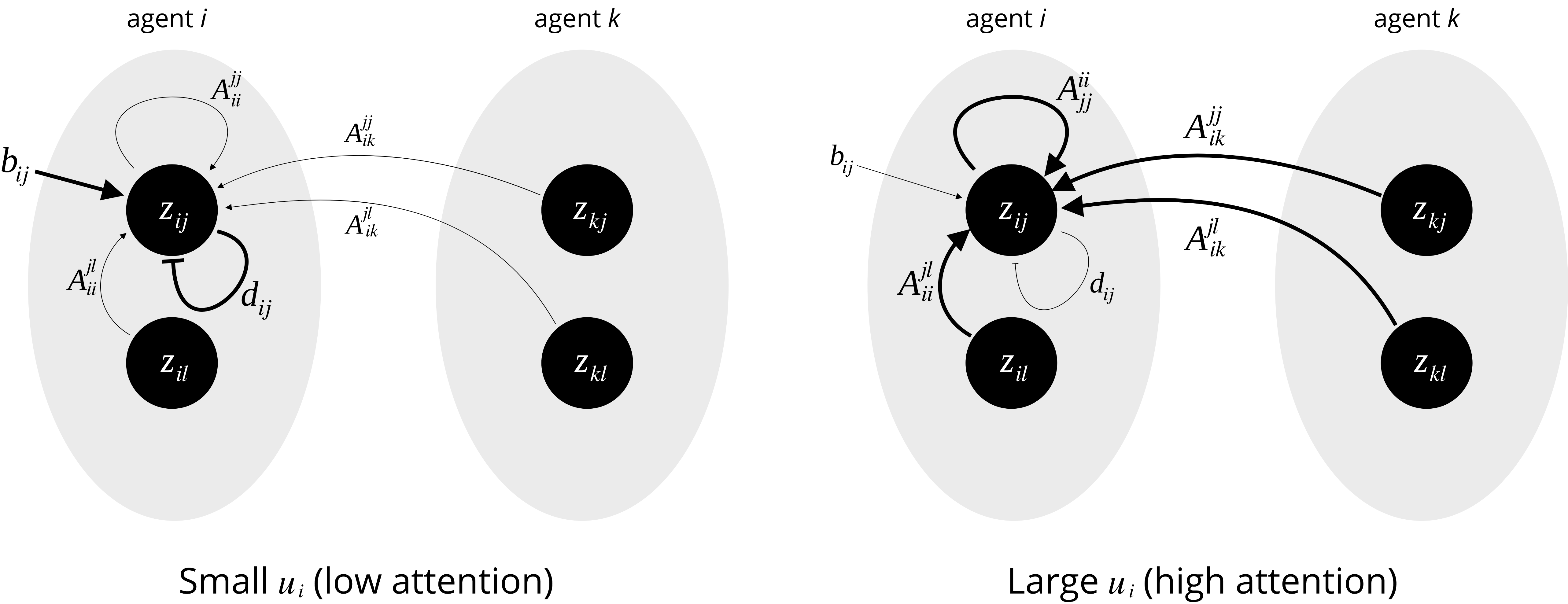
Figure 1: Schematic model description.

In the linear regime, an agent develops an opinion proportional to the ratio of its inputs and its resistance, much like a classical leaky evidence integrator (Bogacz, 2007). In the nonlinear regime, much richer network opinion formation behaviors can be expected. Model (2) was inspired by and specializes to the honeybee-inspired model in Gray et al. (2018). See also Bizyaeva et al. (2020a) for a discussion of the similarities and difference between model (2) and previous opinion formation models in the literature.

2.1 Agreement and disagreement opinion formations are determined by network spectral properties

Model (2) contains hundreds of intrinsic and interaction parameters when ${N_{\rm a}}$ and/or ${N_{\rm o}}$ are sufficiently large. As such, it is intractable in general. However, the model-independent theory in Franci et al. (2020) shows that even in the simplest case in which all four types of network interaction are all-to-all and homogeneous, inputs are zero, attention is uniform across the agents, and the resistance is the same for all the agents, a plethora of rich prototypical opinion formations are still possible in model (2).

To study the role of complex inter-agent network interactions, while preserving analytical tractability, we consider the homogeneous regime of model (2), defined by imposing the following restrictions on the model parameters:

$$d_{ij} =d>0,\ u_{i}=u,\ A_{ii}^{jj}=\alpha\in\mathds{R}$$

$$A_{ii}^{jl} =\beta\in\mathds{R},\ A_{ik}^{jj}=\gamma\tilde{a}_{ik},\ A_{ik}^{jl}=\delta\tilde{a}_{ik}$$ (3)

where $\alpha,\beta,\gamma,\delta\in\mathds{R}$ and $\tilde{a}_{ik}\in\{0,1\}$, for all $i,k=1,\ldots,{N_{\rm a}}$, $i\neq k$, and for all $j,l=1,\ldots,{N_{\rm o}}$, $j\neq l$. The resulting dynamics are

$$\quad\;\;\;\dot{z}_{ij}=F_{ij}(\boldsymbol{Z})-\frac{1}{{N_{\rm o}}}\sum_{l=1}^{{N_{\rm o}}}F_{il}(\boldsymbol{Z})$$ (4a)

$$F_{ij}(\boldsymbol{Z})=-dz_{ij}+u\left(S_{1}\left(\alpha z_{ij}+\sum_{\begin{subarray}{c}k\neq i\\ k=1\end{subarray}}^{N_{\rm a}}\gamma\tilde{a}_{ik}z_{kj}\right)+\sum_{\begin{subarray}{c}l\neq j\\ l=1\end{subarray}}^{N_{\rm o}}S_{2}\left(\beta z_{il}+\sum_{\begin{subarray}{c}k\neq i\\ k=1\end{subarray}}^{N_{\rm a}}\delta\tilde{a}_{ik}z_{kl}\right)\right)+b_{ij}.$$ (4b)

In this regime, the intra-agent network is all-to-all and homogeneous, with weight $\alpha$ for same-option interactions and weight $\beta$ for inter-option interactions. The topology of the inter-agent network is encoded in the adjacency matrix $\tilde{A}=[\tilde{a}_{ik}]\in{\mathds{R}}^{N_{\rm a}}\times{\mathds{R}}^{N_{\rm a}}$. For all existing inter-agent links, i.e., those satisfying $\tilde{a}_{ik}=1$, the inter-agent same-option weight is $\gamma$ and the inter-agent inter-option weight is $\delta$. It is natural to assume that

$$\alpha\geq 0,\quad\text{and}\quad\beta<0,$$ (5)

which means that opinions are self-reinforcing ($\alpha\geq 0$) and mutually exclusive ($\beta<0$). The two remaining parameters, $\gamma$ and $\delta$, determine whether agents cooperate or compete in forming opinions. More precisely, if $\gamma>\delta$, agents cooperate in forming opinions, since the opinion of any agent $i$ about any option $j$ is more strongly excited by the opinions of its neighbors about the same option $j$ than by their opinions about all the other options $l\neq j$. Conversely, if $\gamma<\delta$, agents compete in forming opinions, since the opinion of any agent $i$ about any option $j$ is more strongly excited by the opinions of its neighbors about all the other options $l\neq j$ than by their opinions about the same option $j$.

Remark 1

Because intra-agent coupling is all-to-all and homogeneous in model (4), options are indistinguishable from a network topology perspective. A natural extension of model (4) would be to consider a topologically richer intra-agent network. This generalization is natural in the presence of distinguished options or “issues", i.e., subgroups of more tightly related options.

For homogeneous networks, the cooperative or competitive nature of agent interactions is the key determinant of the opinion formation behavior. The proof of the following theorem follows by linearizing the opinion dynamics (4) at the neutral equilibrium and by studying the kernel of the resulting Jacobian matrix (see (Bizyaeva et al., 2020b, Theorem 1) for details). Let ${\mathds{R}}\{v_{1},\ldots,v_{k}\}$ be the span of vectors $v_{1},\ldots,v_{k}\in{\mathds{R}}^{n}$ and $\mathbf{1}_{n}^{\perp}$ be the orthogonal complement to the vector of ones in ${\mathds{R}}^{n}$.

Theorem 2.1

Suppose that $b_{ij}=0$ for all $i=1,\ldots,{N_{\rm a}}$ and all $j=1,\ldots,{N_{\rm o}}$.

• If $\gamma>\delta$, then in model (4) opinion formation emerges as a bifurcation from the neutral state for

  $$u=u_{a}:=\frac{d}{\alpha-\beta+\lambda_{max}(\gamma-\delta)}$$ (6)

  where $\lambda_{max}$ is the maximum eigenvalue of $\tilde{A}$. All bifurcation branches are tangent to the $({N_{\rm o}}-1)$-dimensional kernel ${\mathds{R}}\{v_{max}\}\otimes\mathbf{1}_{{N_{\rm o}}}^{\perp}$, where $v_{max}$ is the positive (Perron-Frobenius) eigenvector associated to $\lambda_{max}$. More precisely, each bifurcation branch is tangent to a one-dimensional subspace ${\mathds{R}}\{v_{max}\otimes v_{ax}\}$ of ${\mathds{R}}\{v_{max}\}\otimes\mathbf{1}_{{N_{\rm o}}}^{\perp}$, for some $v_{ax}\in\mathbf{1}_{{N_{\rm o}}}^{\perp}$. In particular, because every agent’s opinion state is directly proportional (according to the entries of $v_{max}$) to the same opinion configuration vector $v_{ax}$, all the opinion-formation bifurcation branches are of agreement type.

• If $\gamma<\delta$ and the minimum eigenvalue of $\tilde{A}$ is simple, then in model (4) opinion formation emerges as a bifurcation from the neutral state for

  $$u=u_{d}:=\frac{d}{\alpha-\beta+\lambda_{min}(\gamma-\delta)}$$ (7)

  where $\lambda_{min}$ is the minimum eigenvalue of $\tilde{A}$. All bifurcation branches are tangent to the $({N_{\rm o}}-1)$-dimensional kernel ${\mathds{R}}\{v_{min}\}\otimes\mathbf{1}_{{N_{\rm o}}}^{\perp}$, where $v_{min}$ is the eigenvector associated to $\lambda_{min}$. Each bifurcation branch is tangent to a one-dimensional subspace ${\mathds{R}}\{v_{min}\otimes v_{ax}\}$ of ${\mathds{R}}\{v_{min}\}\otimes\mathbf{1}_{{N_{\rm o}}}^{\perp}$, for some $v_{ax}\in\mathbf{1}_{{N_{\rm o}}}^{\perp}$. Because the vector $v_{min}$ is orthogonal to $v_{max}$, it has mixed-sign entries. In particular, some agents have opinion state directly proportional to the opinion configuration vector $v_{ax}$, whereas some agents have opinion state inversely proportional to it, and so all the opinion-formation bifurcation branches are of disagreement type.

Proof

Equations (6) and (7) were derived in Bizyaeva et al. (2020a)[Theorem IV.1] and Bizyaeva et al. (2020b)[Theorem 1]. The form of the one-dimensional subspaces along which agreement and disagreement bifurcations occur, in particular, the vectors $v_{ax}$, can be constructed using equivariant bifurcation theory methods (Golubitsky et al., 1988; Golubitsky and Stewart, 2002). Because the intra-agent opinion network is all-to-all and homogeneous, model (4) is symmetric with respect to arbitrary option permutations, i.e., it is ${\mathbf{S}}_{N_{\rm o}}$-equivariant, where ${\mathbf{S}}_{N_{\rm o}}$ is the symmetric group of order ${N_{\rm o}}$. It follows from the Equivariant Branching Lemma (Golubitsky et al., 1988, Therem XIII.3.3) that, generically, $v_{ax}$ is the generator of the fixed point subspace of one of the axial subgroups of the action of ${\mathbf{S}}_{N_{\rm o}}$ on $\mathbf{1}_{{N_{\rm o}}}^{\perp}$. There is, of course, only one (modulo multiplication by a non-zero scalar) such vector for ${N_{\rm o}}=2$, i.e., $v_{ax}=(1,-1)$. Modulo multiplication by a non-zero scalar, there are three such vectors for ${N_{\rm o}}=3$, i.e., $v_{ax}=(1,1,-2)$, $v_{ax}=(1,-2,1)$, $v_{ax}=(-2,1,1)$. The form of $v_{ax}$ for $N_{o}>3$ can be similarly derived.

Although derived for the simplified homogeneous dynamics (4), Theorem 2.1 is predictive of the model behavior in the presence of small heterogeneities in the coupling parameter, i.e., when the homogeneous regime is weakly violated. Also, the same bifurcation techniques used to prove this theorem generalize to the case in which large heterogeneities are present. See, e.g., (Bizyaeva et al., 2020a, Section III.C) for a general clustering result in the presence of large difference in the coupling parameter between two or more agent subpopulations.

Remark 2

In (4), we can bring the sums appearing inside $S_{1}$ and $S_{2}$ outside of the sigmoids without changing the qualitative behavior of the model. In particular, because the model Jacobian does not change if sums and sigmoids are swapped, Theorem 2.1 remains true.

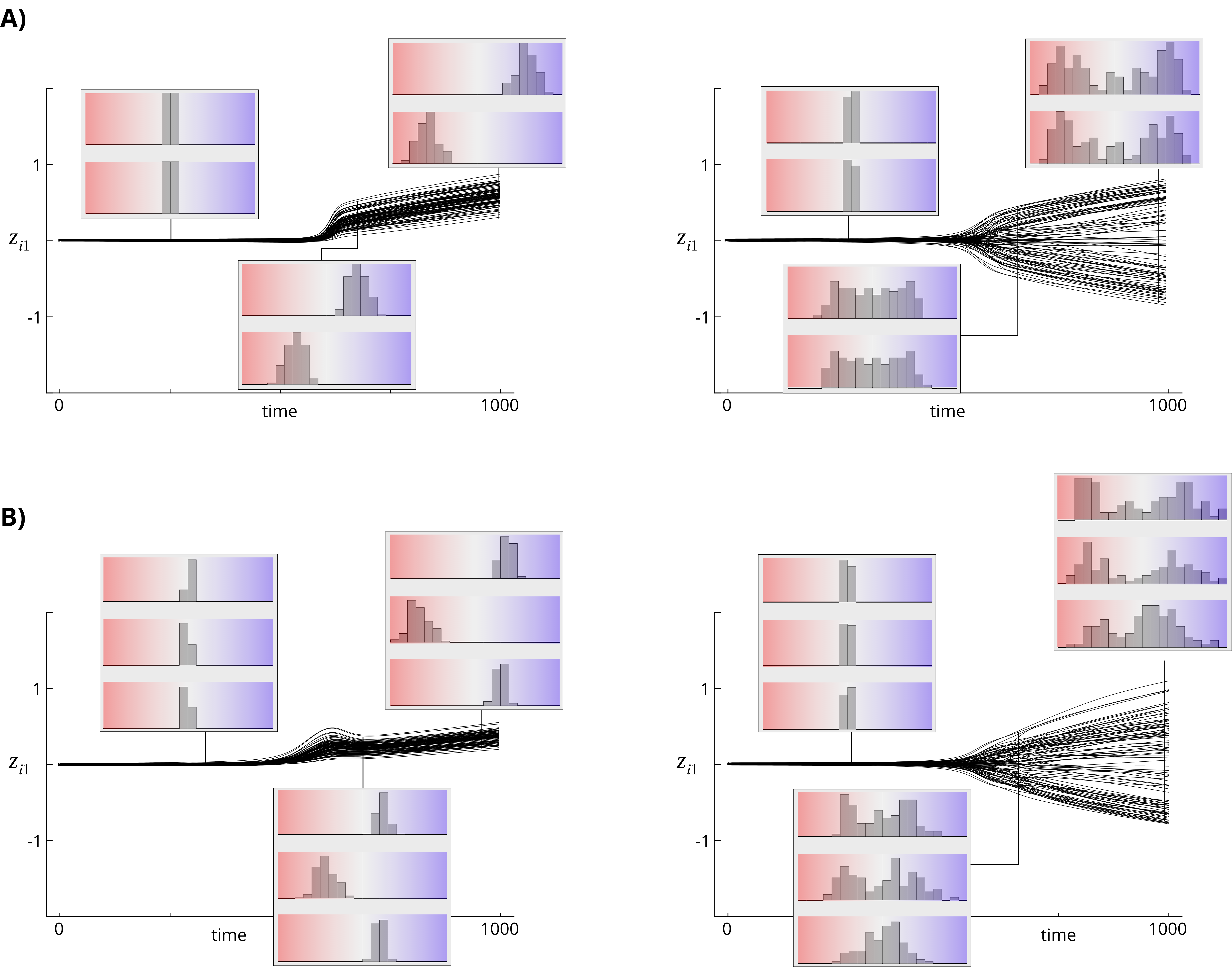
Figure 2: Agreement (left) and disagreement (right) opinion formation in Watts-Strogatz networks with ${N_{\rm a}}=100$ agent nodes and (A) ${N_{\rm o}}=2$ and (B) ${N_{\rm o}}=3$ options. The Watts-Strogatz rewiring probability is $0.9$. Other parameters: $\alpha=0.2$, $\beta=-0.5$, $\gamma=-\delta=0.1$ (agreement), $\gamma=-\delta=-0.1$ (disagreement). Initial conditions and inputs are drawn from a normal distribution with zero mean and variance $10^{-3}$. In all the simulations, $S_{1}(x)=\tanh(x+0.5\tanh(x^{2}))$ and $S_{2}(x)=0.5\tanh(2x+\tanh(x^{2}))$.

In Figures 2 and 3, we illustrate the prediction of Theorem 2.1 for two types of (undirected) complex networks: a Watts-Strogatz “small-world” network (Watts and Strogatz, 1998) and a Barabasi-Albert “scale-free” network (Albert and Barabási, 2002), respectively. Panel A of both figures corresponds to ${N_{\rm o}}=2$ and panel B to ${N_{\rm o}}=3$. In the left plots of each panel, agents are cooperative, whereas in the right plots, agents are competitive. In all the simulations ${N_{\rm a}}=100$ and small Gaussian-distributed random perturbations were added to all inputs $b_{ij}$ to verify the robustness of the theory. Theorem 2.1 is indeed valid for $b_{ij}=0$ but, by normal hyperbolicity of the predicted bifurcation branches of agreement and disagreement equilibria, its predictions remain valid in the case where the $b_{ij}$ are not exactly zero or other types of perturbations (e.g., coupling weights perturbations that weakly violate the homogeneous regime assumption) are present. Precise robustness bounds can be computed using the methods introduced in Wang and Michel (1994). This observation makes Theorem 2.1 relevant for real-world applications.

Each plot in Figures 2 and 3 shows the temporal evolution of $z_{i1}$, i.e., agent $i$’s opinion about the first option, as the attention parameter is slowly increased from below to above the agreement and disagreement opinion-formation critical values $u_{a}$ and $u_{d}$ defined in (6) and (7), respectively. The critical value is reached at half of the simulation time. The insets show the distribution of agent opinions about all the options at one third of the simulation time (i.e., before the opinion forming bifurcation), two thirds of the simulation time (i.e., right after the opinion-forming bifurcation), and at the end of the simulation time. The first (second, third) line shows the distribution of the agent opinions about the first (second, third) option. Colors indicate the strength of favor/disfavor for a given option, with light blue (resp., red) indicating weak favor (resp. disfavor) and dark blue (resp., red) indicating strong favor (resp., disfavor). Asymmetric distributions on the right (left) indicate that agents agree in favoring (disfavoring) the option. A roughly symmetric distribution indicates disagreement about an option, with some agents favoring it and other agents disfavoring it. A sharply bimodal distribution corresponds to polarization of opinions about the option.

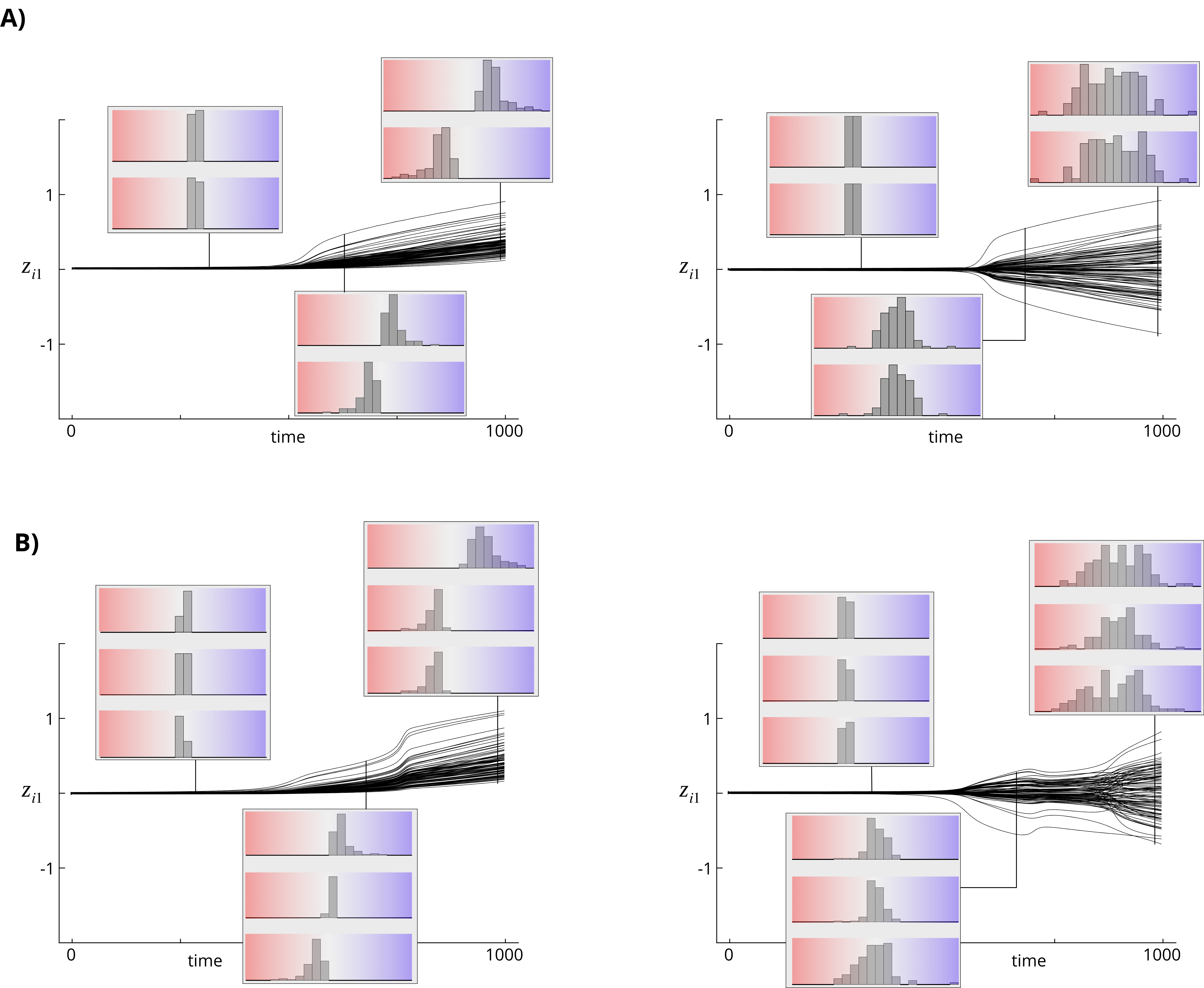
Figure 3: Agreement (left) and disagreement (right) opinion formation in Barabasi-Albert networks with ${N_{\rm a}}=100$ agent nodes and (A) ${N_{\rm o}}=2$ options and (B) ${N_{\rm o}}=3$ options. The Watts-Strogatz rewiring probability is $0.9$. Other parameters: $\alpha=0.2$, $\beta=-0.5$, $\gamma=-\delta=0.1$ (agreement), $\gamma=-\delta=-0.1$ (disagreement). Initial conditions and inputs are drawn from a normal distribution with zero mean and variance $10^{-3}$.

The model behavior follows our theoretical predictions. When agents cooperate, the neutral equilibrium bifurcates at $u=u_{a}$ into an agreement branch where all the agents share the same qualitative opinion. The larger is $u$ relative to $u_{a}$, the stronger are the emerging opinions. In Figures 2A and 3A, left, all the agents favor Option 1 and disfavor Option 2. In Figure 2B, left, all agents disfavor Option 2 and are conflicted between Options 1 and 3. In Figure 3B, left, all agents favor Option 1 and are conflicted between Options 2 and 3. Conversely, when agents compete, the bifurcation branches emerging from the neutral equilibrium are of disagreement type and again opinion strength increases as $u$ increases above $u_{d}$. In Figures 2A and 3A, right, roughly half of the agents favor Option 1, while the other half favor Option 2. In Figures 2B and 3B, right, for each of the three options the group is roughly split into agents that favor the option and agents that disfavor it.

Remark 3

The precise effect of the inputs $b_{ij}$ on the bifurcation and steady-state behavior can be computed using Lyapunov-Schmidt reduction techniques (Golubitsky and Schaeffer, 1985). More precisely, the projection of the input vector onto the bifurcation kernel predicts, to first order, in which direction along the one-dimensional kernel’s subspaces, $\mathbb{R}\{v_{max}\otimes v_{ax}\}$ (agreement case) or $\mathbb{R}\{v_{min}\otimes v_{ax}\}$ (disagreement case) defined in Theorem 2.1, the agreement or disagreement bifurcation unfolds (see (Gray et al., 2018, Theorem 1) for the agreement, 2-option case). At bifurcation, the unfolding direction determines which options are favored or disfavored by the inputs (see, e.g., (Gray et al., 2018, Figure 2)). Here we generalize  (Gray et al., 2018, Theorem 1) to the disagreement and 3-option cases.

3 Multi-Robot Task Allocation as Disagreement Opinion Formation

We illustrate using a detailed example how our opinion dynamics (4) can be applied in robot swarm coordination and control, in particular, to a distributed task-allocation problem. Given its dynamical nature and the small number of parameters, the proposed distributed control algorithm can be implemented in analog circuits and is thus a good candidate for low-computational-power robot swarms that require dynamic task allocation. A single-agent motivation dynamics framework was also recently proposed and applied to a task coordination problem for a mobile robot (Reverdy and Koditschek, 2018; Reverdy et al., 2021). In the spirit of these works, the distributed opinion dynamics of Bizyaeva et al. (2020a) allows us to move beyond a single robotic unit and consider distributed task coordination in a robotic swarm.

Consider that a robot swarm is given ${N_{\rm o}}$ tasks to complete, in which each task has a distinct priority level and each robot may have its own preference to work on certain tasks. To formalize, we denote by a positive constant $\mu_{j}\in[0,1]$, $j=1,\ldots,{N_{\rm o}}$, satisfying $\sum_{j=1}^{N_{\rm o}}\mu_{j}=1$, the priority of each task $j$. The main objective in this example is to design a simple distributed decision-making algorithm that assigns robots to each task. The algorithm should be designed to respect task priority, i.e., the larger the task priority $\mu_{j}$, the larger the number of robots assigned to that task by the algorithm.

Given an undirected communication network between the robots, with adjacency matrix $[\tilde{a}_{ik}]_{i,k=1}^{N_{\rm a}}$, let $\mathcal{N}_{i}$ be set of neighbors of robot $i$. We adapt opinion dynamics (4) to the task-allocation problem as follows. The preference that robot $i$ gives to performing task $j$ evolves accordingly to vector field

$$\dot{z}_{ij} =F_{ij}(\mathbf{Z})-\frac{1}{N_{o}}\sum_{l=1}^{N_{o}}F_{il}(\mathbf{Z})$$ (8a)

$$F_{ij}(\mathbf{Z}) =-z_{ij}+u\,\left(\mu_{j}\,(|\mathcal{N}_{i}|+\nu_{ij})-\frac{1}{2}\sum_{k\in\mathcal{N}_{i}}S\left(2\tilde{\gamma}z_{kj}\right)\right).$$ (8b)

The positive parameter $\nu_{ij}$ is the intrinsic zealousness of robot $i$ to perform task $j$. As we will see, the zealousness parameter can be used as control input to the robot swarm to trigger the distributed task allocation. Opinion dynamics (4) specialize to model (8) by letting $b_{ij}=u\mu_{j}(|\mathcal{N}_{i}|+\nu_{ij})$, $\alpha=\beta=\delta=0$, $\tilde{\gamma}=-\gamma>0$, and by swapping the inter-agent interaction sum with the sigmoid $S_{1}$ (as discussed in Remark 2, this choice does not affect the qualitative behavior of the model).

The rationale behind the derivation of model (8) is the following. Let $N_{i}^{j}$ be the number of robots in $\mathcal{N}_{i}$ that express preference for task $j$, i.e., such that $z_{kj}>0$. Because generically $z_{kj}\neq 0$ and if the upper and lower limits of $S$ are $\pm 1$, respectively, for sufficiently large $\gamma$ the term $\frac{1}{2}\sum_{k\in\mathcal{N}_{i}}S\left(2\gamma z_{kj}\right)\approx\frac{1}{2}\left(N_{i}^{j}-\left(|\mathcal{N}_{i}|-N_{i}^{j}\right)\right)=N_{i}^{j}-\frac{|\mathcal{N}_{i}|}{2}$. Imposing the simplex condition by subtracting the average opinion drift as in (8a), the constant $\frac{|\mathcal{N}_{i}|}{2}$ disappears from the opinion dynamics on the simplex and, for $\nu_{ij}=0$ the effective interaction term reduces to

$$\mu_{j}\,|\mathcal{N}_{i}|-\frac{1}{2}\sum_{k\in\mathcal{N}_{i}}S\left(\epsilon z_{kj}\right)\approx\mu_{j}\,|\mathcal{N}_{i}|-N_{i}^{j}\,.$$ (9)

In other words, in our task-allocation model, each robot updates its preference for task $j$ roughly proportionally to the priority of task $j$, scaled by the number of its neighbors, minus the number of its neighbors that already show a preference for the same task. A non-zero zealousness $\nu_{ij}$ increases the tendency of robot $i$ to choose task $j$.

Observe that the condition $-\tilde{\gamma}=\gamma<0$ and $\delta=0$ imposes that the model is in the disagreement regime for $u>u_{d}>0$. Thus, in our model, the robots naturally develop different opinions about the tasks, i.e., they self-allocate across the task in a distributed fashion. Furthermore, robot task-allocation will reflect task priorities, which, from a bifurcation viewpoint, breaks the symmetry between the tasks.

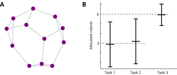
Figure 4: A. The Frucht Graph. B. Average (large bar) and standard deviation (short bar) of the number of agents allocated to Tasks 1,2,3 over one-hundred instances of our task-allocation algorithm. Details in the main text.

We illustrate the performance of our task-allocation algorithm for a swarm of ${N_{\rm a}}=12$ robots allocating themselves across ${N_{\rm o}}=3$ tasks. We assume that the inter-agent communication graph is the Frucht graph (Frucht, 1939) (see Figure 4A), which is 3-regular ($|\mathcal{N}_{i}|=3$ for all $i=1,\ldots,{N_{\rm a}}$) but possesses no non-trivial symmetries, i.e., all robots can be distinguished by their position in the graph. Our algorithm is particularly suited in a priori deadlocked situations, i.e., those in which two or more tasks have the same objective priority. In our example, we set $\mu_{1}=\mu_{2}=0.3$ and $\mu_{3}=0.4$. We also set $\tilde{\gamma}=1.0$ and $u=2u_{d}$. For the sigmoid function we use $S(x)=\tanh(x+0.5\tanh(x^{2}))$, where the $\tanh(x^{2})$ ensure genericity (i.e., non-vanishing even partial derivatives) of the $S$ at the origin. We run one hundred repetitions of our example with small random zealousness parameters $\nu_{ij}$ (modeling parametric uncertainties) and small random initial conditions, and computed the resulting average and standard deviation of the number of robots allocated to each option.

Robot $i$ is considered allocated to task $j$ if at the end of the simulation $\|\boldsymbol{Z}_{i}\|\geq\theta$ and $z_{ij}>z_{il}$ for all $l\neq j$, where $\theta$ is a control threshold parameter that determines whether a robot became opinionated (in the simulations, $\theta=0.1$). The final simulation time can be considered as a tunable decision deadline for the task-allocation decision. Figure 4B shows the results of our analysis. On average, a larger number of agents is allocated to the highest-priority task. A roughly equal number of agents is allocated on average to the less urgent tasks. The standard deviation of the allocation number is also smaller for the highest-priority task, which indicates that our algorithm consistently allocates the largest number of robots to the highest-priority task. Of course, there is a lot of room for improving the simple algorithm proposed in this section, in particular, in order to drastically reduce variability in the number of agents allocated to the various tasks, and thus increase robustness to initial conditions and parameter uncertainties. In some instances of our example, depending on initial conditions or the intrinsic zealousness parameters, no robots were allocated to either Task 1 or Task 2, which is clearly an undesirable situation in practice. We suggest a strategy to overcome these limitations in Section 6.

4 Opinion cascades with tunable sensitivity from feedback attention dynamics

In this section we couple the opinion dynamics (4) with the attention dynamics introduced in  Bizyaeva et al. (2020a). Using a detailed geometrical analysis for the case ${N_{\rm o}}=3$ (the case ${N_{\rm o}}=2$ is studied in Bizyaeva et al. (2020a)), we show that the resulting positive feedback between attention and opinion strength allows an agent to transition from being in a stable unopinionated state to a stable opinionated state in response to an input $\mathbf{b}_{i}=(b_{i1},\ldots,b_{iN_{o}})$ sufficiently large in magnitude. The associated activation threshold is implicitly defined by the geometric properties of the dynamics and is explicitly tunable with the model parameters. The threshold effect mediated by the positive feedback between attention and opinion strength scales up to networks of interconnected agents under the influence of inputs on a small number of “seed nodes". At the network level, the coupling between opinion and attention dynamics creates a threshold for the input magnitude below which the network remains close to neutral and above which an opinion cascade is triggered.

4.1 Feedback attention dynamics and tunable sensitivity of opinion formation at the single agent level

To understand the effect of coupled opinion and attention dynamics we first consider an agent without any neighbors. Even without an inter-agent communication network, the dynamics of each agent’s opinions are organized by a bifurcation at which the agent develops preferences for the available options. When $\tilde{a}_{ik}=0$ for all $i,k=1,\dots,N_{a}$, the $F_{ij}(\boldsymbol{Z})$ function in (4b) becomes

$$F_{ij}(\boldsymbol{Z})=-dz_{ij}+u_{i}\left(S_{1}\left(\alpha z_{ij}\right)+\sum_{\begin{subarray}{c}l\neq j\\ l=1\end{subarray}}^{N_{\rm o}}S_{2}\left(\beta z_{il}\right)\right)+b_{ij}.$$ (10)

When $b_{ij}=0$, for all $j=1,\dots,N_{o}$, and $u_{i}<\frac{d}{\alpha-\beta}$, the neutral opinion state $\boldsymbol{Z}_{i}=\mathbf{0}$ of agent $i$ is stable. At $u_{i}^{*}=\frac{d}{\alpha-\beta}$ branches of opinionated solutions emerge in an $S_{N_{o}}$-equivariant bifurcation, which is studied in detail in Elmhirst (2004). We omit the formal details of this bifurcation analysis here, and simply note that for $u_{i}<u_{i}^{*}$ the agent’s opinion converges to the neutral equilibrium with $\|\boldsymbol{Z}_{i}^{*}\|=0$, whereas for $u_{i}>u_{i}^{*}$ it converges to some nonzero magnitude equilibrium $\|\boldsymbol{Z}_{i}^{*}\|>0$, whose norm grows monotonically with $u_{i}$. The stable opinionated equilibria that appear as primary bifurcation branches correspond either to agent $i$ choosing one option and rejecting all others, or to it being conflicted between a subset of the available options (Figure 5A, left).

The dynamics of an agent $i$’s opinion with nonzero input $\mathbf{b}_{i}$ directly follow from the bifurcation behavior of its opinion dynamics with $\mathbf{b}_{i}=\mathbf{0}$. As discussed in Section 2, when $u_{i}$ is small, the input $\mathbf{b}_{i}$ and resistance $d$ define the linear opinion formation behavior of agent $i$. For large $u_{i}$ the nonlinear behavior dominates and agent $i$’s opinion can become much larger in magnitude than its input $\mathbf{b}_{i}$. Generically, when $\mathbf{b}_{i}\neq 0$, for values of $u_{i}$ near $u_{i}^{*}$, a single branch of stable opinionated solutions is selected accordingly to ${\mathbf{b}}_{i}$, while all other solutions are removed (Figure 5A, right).

How the opinion bifurcation diagram changes in response to inputs motivates the design of an attention feedback dynamic that increases an agent’s attention from below to above its bifurcation point when sufficiently large inputs are present. We define the closed-loop attention dynamics as

$$\tau_{u}\dot{u}_{i}=-u+u_{min}+(u_{max}-u_{min})S_{u}(\|\boldsymbol{Z}_{i}\|)$$ (11)

where $\tau_{u}$ is an integration timescale and $S_{u}:{\mathds{R}}_{\geq 0}\to[0\ 1]$ is a smooth saturating function, satisfying $S_{u}(0)=0$, $S_{u}(y)\to 1$ as $y\to\infty$, $S_{u}^{\prime}(y)>0$ for all $y\in{\mathds{R}}_{\geq 0}$, $S^{\prime\prime}_{u}(y)>0$ for all $0\leq y<u_{th}$ and $S^{\prime\prime}_{u}(y)<0$ for all $y>u_{th}$, with $u_{th}>0$. For the sake of numerical illustrations we use $S_{u}(y)=\frac{y^{n}}{u_{th}^{n}+y^{n}}$. The larger is $n$ the steeper is the sigmoid around its threshold $u_{th}$. We assume $u_{min}<u_{i}^{*}<u_{max}$ and $n$ sufficiently large so that the saturation is sufficiently steep.

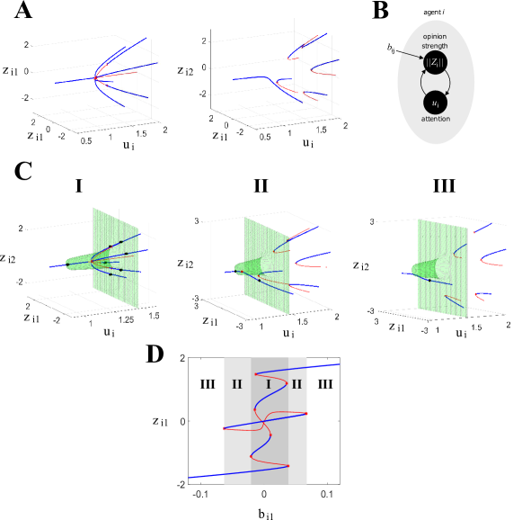
Figure 5: A. Bifurcation diagram of the single agent dynamics with respect to the attention parameter. Left: ${\mathbf{b}}_{i}=0$. Right: ${\mathbf{b}}_{i}\neq 0$. B. Schematic of the relationship between an agent’s opinion strength, attention, and input. C. Representative intersections of the attention nullclines (green surface) and opinion nullclines (red and blue lines) for the three parameter regimes with $N_{o}=3$. D. Bifurcation diagram of the coupled system (10),(11) with $N_{o}=3$, projected to the $b_{i1}$, $z_{i1}$ plane. In D blue (red) lines correspond to stable (unstable) equilibria of the coupled system. In A,C blue (red) lines correspond to stable (unstable) equilibria of the opinion dynamics (10) with a static attention parameter. Additional branches of unstable equilibria are not shown in A,C-I for diagram clarity. Black (red) spheres mark the stable (unstable) equilibria of the coupled system. Parameters: $d=1$, $\alpha=0.4$, $\beta=-0.4$, $u_{min}=1.05$, $u_{max}=1.45$, $n=3$, $u_{th}=0.15$. B: $b_{i2}=0.005,b_{i3}=-0.002$, $b_{i1}$ varied as illustratd. A (left) and CI: $\mathbf{b}_{i}=0$; A (right) and CII : $\mathbf{b}_{i}=(0.05,-0.01,0.02)$; CIII: $\mathbf{b}_{i}=(0.1,-0.01,0.02)$. Diagrams in A,C,D are generated with help of MatCont numerical continuation package (Dhooge et al., 2008).

The closed-loop attention dynamics (11) create a localized positive feedback between an agent’s attention and its opinion strength, as illustrated in Fig. 5B. We use the chain rule to compute partial derivatives at $\boldsymbol{Z}_{i}=0$ of the time-derivative of $z_{ij}^{2}$ with respect to attention $u_{i}$ of an agent whose dynamics are defined by (11) and, conversely, the time-derivative of $u_{i}$ (11) with respect to $z_{ij}^{2}$. The sign of the product of these two partial derivatives gives the sign of the feedback between attention and opinion strength at the neutral equilibrium. Computing, we get

$$\frac{\partial\dot{(z_{ij}^{2})}}{\partial u_{i}} =2z_{ij}\left(\frac{N_{o}-1}{N_{o}}\Big{(}S_{1}(\alpha z_{ij})-S_{2}(\beta z_{ij})\Big{)}-\frac{1}{N_{o}}\sum_{\begin{subarray}{c}l\neq j\\ l=1\end{subarray}}^{N_{o}}\Big{(}S_{1}(\alpha z_{il})-S_{2}(\beta z_{il})\Big{)}\right),$$

$$\frac{\partial\dot{u}_{i}}{\partial(z_{ij}^{2})} =\frac{1}{\tau_{u}}(u_{max}-u_{min})S_{u}^{\prime}(\|\boldsymbol{Z}\|).$$

Near the neutral equilibrium $\boldsymbol{Z}_{i}=0$ we can approximate $S_{1}(\alpha z_{il})-S_{2}(\beta z_{il})\approx(\alpha-\beta)z_{il}$, and using the simplex constraint on the opinions we find that for small $\boldsymbol{Z}_{i}$ and any $j=1,\dots,N_{o}$, $\frac{\partial\dot{(z_{ij}^{2})}}{\partial u_{i}}\approx 2(\alpha-\beta)z_{ij}^{2}$. Therefore

$$\frac{\partial\dot{(z_{ij}^{2})}}{\partial u_{i}}\frac{\partial\dot{u}_{i}}{\partial(z_{ij}^{2})}\approx\frac{2}{\tau_{u}}(\alpha-\beta)(u_{max}-u_{min})z_{ij}^{2}S_{u}^{\prime}(\|\boldsymbol{Z}\|).$$ (12)

The right-hand side of (12) is positive whenever $z_{ij}\neq 0$. Thus, a positive feedback loop between an agent’s opinion strength and its attention is triggered as soon as its opinion deviates from zero.

The localized positive feedback between attention and opinion strength creates multistability and threshold behavior in the closed-loop opinion dynamics. Figures 5C and 5D illustrate the three-dimensional phase portrait and the steady-state behavior (bifurcation diagram) of the closed-loop opinion-attention dynamics for ${N_{\rm o}}=3$, respectively. The bifurcation diagram in Fig. 5D is projected onto the $z_{i1}$,$b_{i1}$ plane. Note that the bifurcation diagram characterizes the input-output relationship, where the input is ${\mathbf{b}}_{i}$ and the output is the steady-state opinion.

We can distinguish three regimes (labels as in Fig. 5D):

1. Multistability: $\|\mathbf{b}_{i}^{\perp}\|<\varepsilon_{1}$. For small $\|\mathbf{b}_{i}^{\perp}\|$, the opinion and attention nullclines intersect in many locations and a number of these intersections are stable equilibria. One of the intersections is near to $u_{i}=u_{min}$ and $\boldsymbol{Z}_{i}=\mathbf{0}$ and is stable. The other stable equilibria correspond to intersections of opinionated solution branches with attention nullcline near $u_{i}=u_{max}$. For small initial conditions, agent $i$’s opinion and attention remain small, attracted by the stable equilibrium near to $u_{i}=u_{min}$. For large initial conditions they approach one of the opinionated equilibria. In this parameter regime the initial conditions determine whether agent $i$ becomes opinionated, and also which opinion it forms.

2. Bistability: $\varepsilon_{1}<\|\mathbf{b}_{i}^{\perp}\|<\varepsilon_{2}$. For intermediate $\|\mathbf{b}_{i}^{\perp}\|$, the coupled dynamics admit only two stable equilibria: one is the unopinionated equilibrium near $u_{i}=u_{min}$ and the other is an opinionated equilibrium on the solution branch favored by the input $\mathbf{b}_{i}$. For small initial conditions, agent $i$’s opinion and attention remain small, wherease for large initial conditions they approach the stable equilibrium picked out by the input. In this regime, initial conditions determine whether or not an agent becomes opinionated, but the input governs the opinion formation outcome.

3. Cascade: $\|\mathbf{b}_{i}^{\perp}\|>\varepsilon_{2}$. For sufficiently large $\|\mathbf{b}_{i}^{\perp}\|$, the coupled system has a unique stable equilibrium point which corresponds to an opinionated state favoring the opinion picked out by the input $\mathbf{b}_{i}$. From any initial condition, an agent will reliably become opinionated in the direction informed by the input.

The boundaries $\varepsilon_{1}$, $\varepsilon_{2}$ between these three regimes can be tuned by the parameters of the saturation function $S_{u}$ in (11). In other words, the sensitivity of the closed-loop dynamics to forming opinions in response to inputs is tunable.

4.2 Network opinion cascades with tunable sensitivity

In the presence of symmetric network interactions, the intra-agent positive feedback loop between attention and opinion strength scales up to the network level, as illustrated in Figure 6. Independent of their excitatory or inhibitory nature, network interactions create a positive feedback loop between the opinion strengths of any pair of interconnected agents, at least close to the neutral equilibrium where the interaction nonlinearities are steeper and thus the opinion interaction is stronger. To show this statement we use the chain rule to compute partial derivatives at the neutral equilibrium of the time-derivative of $z_{ij}^{2}$ with respect to $z_{kl}^{2}$ for two agents $i$ and $k$ interacting according to (4) and for symmetric network coupling. Computing, we get

$$\left.\frac{\partial\dot{(z_{ij}^{2})}}{\partial z_{kl}^{2}}\right|_{\boldsymbol{Z}=0}=\frac{1}{{N_{\rm o}}}\frac{z_{ij}}{z_{kl}}u_{i}\tilde{a}_{ik}(\delta-\gamma),\text{ if }l\neq j,\quad\left.\frac{\partial\dot{(z_{ij}^{2})}}{\partial z_{kj}^{2}}\right|_{\boldsymbol{Z}=0}=\frac{{N_{\rm o}}-1}{{N_{\rm o}}}\frac{z_{ij}}{z_{kj}}u_{i}\tilde{a}_{ik}(\gamma-\delta)$$

Thus, if $\tilde{a}_{ik}=1$, by symmetry,

$$\left.\frac{\partial\dot{(z_{ij}^{2})}}{\partial z_{kl}^{2}}\frac{\partial\dot{(z_{kl}^{2})}}{\partial z_{ij}^{2}}\right|_{\boldsymbol{Z}=0}=\frac{1}{{N_{\rm o}}^{2}}u_{i}u_{k}(\gamma-\delta)^{2},\text{ if }l\neq j,\quad\left.\frac{\partial\dot{(z_{ij}^{2})}}{\partial z_{kj}^{2}}\frac{\partial\dot{(z_{kj}^{2})}}{\partial z_{ij}^{2}}\right|_{\boldsymbol{Z}=0}=\left(\frac{{N_{\rm o}}-1}{{N_{\rm o}}}\right)^{2}u_{i}u_{k}(\gamma-\delta)^{2},$$ (13)

which yields an element-wise positive feedback loop between the opinion strengths of agent $i$ and agent $k$. As a consequence, when equations (2) and (11) are coupled, the attention variables of agents $i$ and $k$ are also interconnected in an (indirect) positive feedback loop. This can easily be seen by computing the overall sign of the interconnection loop from $u_{i}$ to $u_{k}$ and back, passing through $||\boldsymbol{Z}_{i}||$ and $||\boldsymbol{Z}_{k}||$ (see Fig. 6). The existence of a networked positive feedback between the agents’ attention variables and opinion strengths suggests the existence of a network threshold for the trigger of opinion cascades.

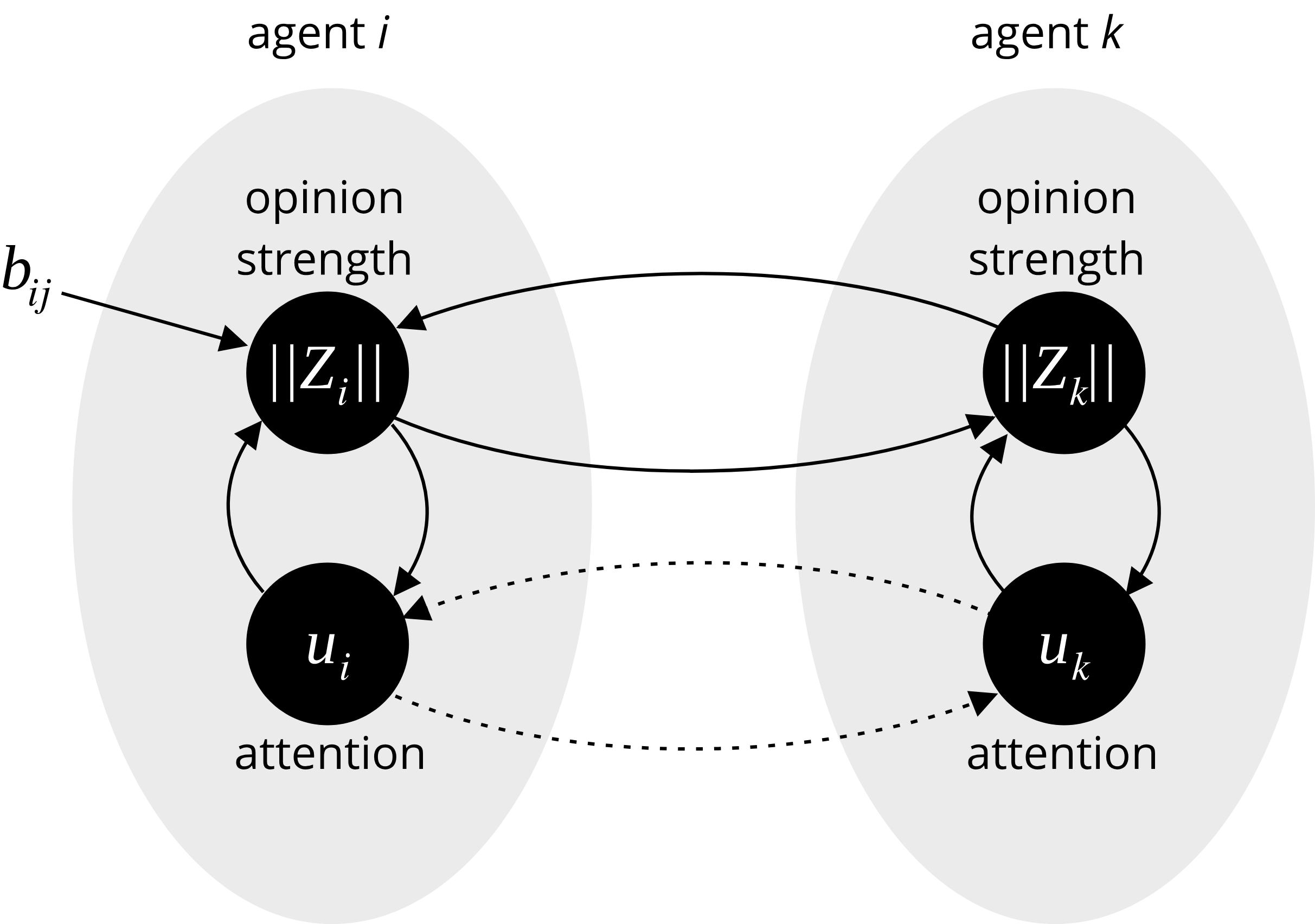
Figure 6: Intra- and inter-agent positive feedback loops between the agents’ opinion strengths and their attention.

An opinion cascade refers to the situation in which only a small number $N_{seeds}\ll{N_{\rm a}}$ of agents, called seeds, receive non-zero inputs $\boldsymbol{b}_{1},\ldots,\boldsymbol{b}_{N_{seeds}}$ and yet a large part of the network develops a markedly non-zero opinion. In the network example of Figure 7A, the cascade seeds are indicated with blue and red arrows depending on the options favored or disfavored by the input (see the figure caption for details). When the inputs to the seeds are small, only the seeds develop clear opinions aligned with their respective inputs, while the other agents remain weakly opinionated or unopinionated in such a way that the network average opinion strength remains small (Figure 7B1). When the inputs to the seeds are sufficiently strong, the seeds develop opinions that are sufficiently strong to engage the positive feedback of the network attention, which spreads to some or all of the rest of the agents with some variable delay. This yields an opinion cascade such that the network average opinion strength grows large (Figure 7B2). Whether the cascade is towards agreement or disagreement depends on the cooperative (left plots) or competitive (right plots) nature of the agents. Observe that in both agreement and disagreement cases, a number of agents have afterthoughts: they develop an early opinion about Option 1 but either exhibit the opposite opinion or become neutral by the end of the cascade process.

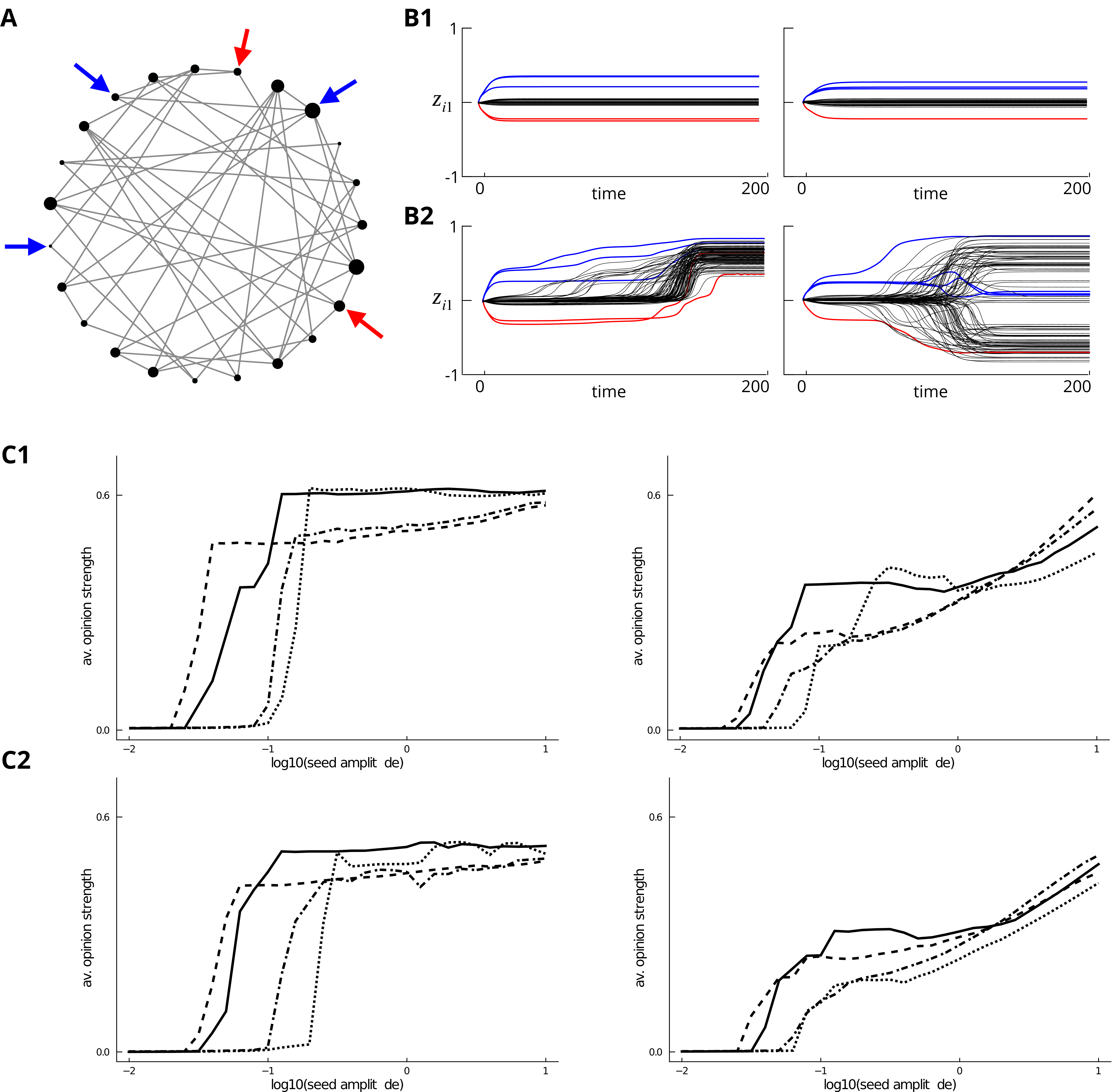
Figure 7: Agreement and disagreement opinion cascades. A. Schematic of the network structure. In a large network, only a small number of agents receive inputs, indicated by arrows. Inputs have the same strength, i.e., the same norm, but they can differ in the information they bring, i.e., which option they favor. In the numerical simulations, inputs are in favor (blue arrows) or in disfavor (red arrows) of Option 1. B. Network response to inputs for cooperative (left) and competitive (right) agents. B1. Small inputs (no cascade). B2. Large inputs (cascade). C. Cascade threshold analysis. The plots show how the average network opinion strength changes as a function of the seed input amplitude (in logarithmic scale) over ten network instances with random seed placement. ${N_{\rm o}}=2$ in C1 and ${N_{\rm o}}=3$ in C2. Left plots: Watts-Strogatz network. Right plots: Barabasi-Albert network. Full lines: cooperative agents, $u_{th}=0.05$. Dashed line: competitive agents, $u_{th}=0.05$. Dotted lines: cooperative agents, $u_{th}=0.1$. Dashed-dotted lines: competitive agents, $u_{th}=0.1$. Other parameters as in Figures 2 (Watts-Strogatz case) and 3 (Barabasi-Albert case). In all simulations, $\delta_{u}=0.2$.

In the following, we fix the number $N_{seeds}$ and let all inputs $\boldsymbol{b}_{1},\ldots,\boldsymbol{b}_{N_{seeds}}$ have the same norm $\bar{b}$ but still allow each to bring information either in favor or in disfavor of Option 1. In the attention dynamics (11), we use $u_{min}=u_{a}-\delta_{u}$ and $u_{max}=u_{a}+\delta_{u}$, where $u_{a}$ is defined in (6), in the agreement (cooperative agents) regime, and $u_{min}=u_{d}-\delta_{u}$ and $u_{max}=u_{d}+\delta_{u}$, where $u_{d}$ is defined in (7), in the disagreement (competitive agents) regime. This choice makes the opinion cascade behavior independent of the network-specific opinion-formation bifurcation point. The network topology, seed placement, seed input amplitude, and the attention threshold $y_{m}$ are thus the only determinants of the observed opinion cascade behavior.

To verify the existence of a network threshold for the trigger of opinion cascades, in Figure 7 we systematically vary network topology, attention threshold, and seed input amplitude, for randomly placed seeds. Figures 7C1 and  7C2 correspond to the case ${N_{\rm o}}=2$ and ${N_{\rm o}}=3$, respectively. All plots show the steady-state average network opinion strength $\frac{1}{{N_{\rm a}}}\sum_{i=1}^{N_{\rm a}}||\boldsymbol{Z}_{i}^{*}||$ as a function of the seed input amplitude in the coupled (4)-(11) system. Right plots are the average results for ten instances of a Watts-Strogatz network with randomly placed seeds and left plots are the average results for ten instances of a Barabasi-Albert network with randomly placed seeds ($N_{seeds}=5$ for both types of network). For each network and each value of ${N_{\rm o}}$, we consider four different regimes: cooperative agents, $y_{m}=0.05$ (full lines); competitive agents, $y_{m}=0.05$ (dashed lines); cooperative agents, $y_{m}=0.1$ (dotted lines); competitive agents, $y_{m}=0.1$ (dashed-dotted lines). In all cases one can detect a threshold value above which distinctively non-zero average opinion emerge, indicating a cascade as in Figures 7B1 and B2.

The cascade threshold increases monotonically with $u_{th}$. The parameter $u_{th}$ tunes cascade sensitivity at the single agent level, in the sense that smaller (larger) values of $u_{th}$ decrease (increase) the minimum input strength necessary to trigger a cascade at the single agent level (Bizyaeva et al., 2020a, Theorem VI.6). In the presence of networked interaction, the tunable cascade sensitivity of the single agent level scales up to the network level: for large $u_{th}$, large seed input strengths are necessary to trigger a cascade; for small $u_{th}$, small seed input strengths are sufficient to trigger a cascade.

Observe that in our model cascades can be partial or complete. For instance, the agreement cascade is complete in Figure 7B2 left because all agents develop a markedly non-zero opinion. Conversely, the disagreement cascade is only partial in Figure 7B2 right because some of the agents, including one of the seeds, possess a roughly neutral opinion at the post-cascade steady state. We further observe that, generically, when the bifurcation parameter is the seeds’ input strength, as considered here, cascades happen through a simple saddle-node bifurcation. It follows that for supra-threshold inputs the time to reach the post-cascade steady state is inversely proportional to the input strength, a phenomenon known in the dynamical system literature as “traversing the ghost of the saddle-node bifurcation" (Izhikevich, 2007, Section 3.3.5). A detailed analysis of both the transition from partial to complete cascades and the time to the post-cascade steady state is left for future developments.

5 Control of agreement and disagreement opinion cascade by input centrality assignment

This section explores how the sensitivity of an opinion-forming network to trigger an agreement or disagreement cascade in response to a small number of inputs can be controlled by exploiting the emergent properties of the network. We introduce notions of agreement and disagreement centrality. These centrality indices can be used to guide the cascade seed placement towards maximizing or minimizing the network response to inputs, independent of the intrinsic node properties like, e.g., the attention threshold parameter $u_{th}$. In other words, our cascade model can be controlled independently and simultaneously in two ways: intrinsically at the agent level, by tuning the attention dynamic parameters, and extrinsically at the network level, by exploiting the network topology for efficient seed placement. We consider extrinsic control that enhances or diminishes sensitivity to inputs for agreement (disagreement) cascades by selecting as seeds the most or least central agents as defined by the agreement (disagreement) centrality index. The selected set of agents is optimal in the case centrality is modular; otherwise, it provides only an approximation to the optimal set of agents (see, for example, (Clark et al., 2014; Fitch and Leonard, 2016)). We save the investigation of optimality for future work.

5.1 Agreement and disagreement centrality

A key prediction of Theorem 2.1 is that the absolute value of the entries of the adjacency matrix’s eigenvectors $v_{max}$ and $v_{min}$ predict (up to linear order) the opinion strength (and sign) of each agent along agreement and disagreement bifurcation branches, respectively. This result suggests the following notion of centrality for agreement and disagreement opinion formation.

Let $\tilde{A}$ be the unweighted adjacency matrix of an undirected, connected network. Let $v_{max}$ be the normalized positive eigenvector associated to the unique maximal eigenvalue of $\tilde{A}$. Assume that the minimal eigenvalue is also unique and let $v_{min}$ be the associated normalized eigenvector.

Definition 1

We define agreement centrality of agent $i$ as $[v_{max}]_{i}$, disagreement centrality of agent $i$ as $|[v_{min}]_{i}|$, and signed disagreement centrality of agent $i$ as $[v_{min}]_{i}$

The proposed notion of agreement centrality is the same notion of eigenvector centrality introduced in Bonacich (1972). The proposed notion of disagreement centrality is new. Both notions of centrality will be key to analyzing and controlling opinion cascades over networks. It makes sense to talk about a signed disagreement centrality because the eigenvector $v_{min}$ has mixed sign entries (whereas $v_{max}$ can always be chosen to be positive). We will show that signed disagreement centrality is instrumental to controlling disagreement opinion cascades. For directed networks, one could use the eigenvectors of $\tilde{A}+\tilde{A}^{T}$ to define suitable centrality indices. We leave these ideas for future investigations.

5.2 Control of agreement opinion cascades by centrality assignment

Suppose that we can choose $N_{seeds}$ agents to receive input, and suppose that each input has the same norm $\bar{b}$, but brings potentially different information (i.e., favoring or disfavoring) about, say, Option 1.

• Towards maximization of agreement cascade sensitivity. Let the control objective be to maximize the sensitivity of agreement opinion cascades to the $N_{seeds}$ inputs. Then an effective approach is to select the cascade seeds to be the $N_{seeds}$ most central agents, according to the agreement centrality.

• Towards minimization of agreement cascade sensitivity. Let the control objective be to minimize the sensitivity of agreement opinion cascades to the $N_{seeds}$ inputs. Then an effective approach is to select the cascade seeds to be the $N_{seeds}$ least central agents, according to the agreement centrality.

The rationale behind the proposed control strategy is the following. Maximally central agents are those that tend to develop stronger opinions at an agreement bifurcation. Triggering the network attention/opinion-strength positive feedback at maximally central agents therefore enhances the network response toward crossing the agreement cascade threshold. Likewise, minimally central agents tend to develop small opinions at an agreement bifurcation. Triggering the network attention/opinion-strength positive feedback at minimally central agents therefore diminishes the network response and keeps it away from crossing the agreement cascade threshold.

We illustrate the effectiveness of our agreement cascade control strategy in an eleven-agent network with $N_{seeds}=2$ and ${N_{\rm o}}=3$. Figure 8A1 shows the network topology and the resulting node agreement centralities (visualized as the node sizes). The two black arrows point to the two most central agents. The two gray arrows point to the two less central agents. All agents have an intrinsic attention threshold $u_{th}=0.1$. When the two inputs affect the two most central agents following our sensitivity-maximization algorithm, inputs with amplitudes as small as $0.1$ are sufficient to trigger a full network cascade with large average opinion strength (Figure 8B1 - black curve) and in which all agents become opinionated (Figure 8C1, top). Conversely, when the two inputs affect the two less central agents following our sensitivity-minimization algorithm, the network is still resisting to trigger a full cascade even for input amplitude as large as $1.0$ (Figure 8B1 - gray curve). Only the two agents receiving an input are opinionated, while the rest of the agents remain close to neutral (Figure 8C1, bottom).

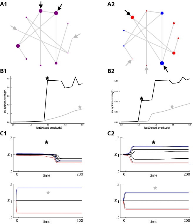
Figure 8: Control of agreement and disagreement opinion cascade by centrality assignment. A1: network topology and agreement centrality. The node size is proportional to its agreement centrality. A2: network topology and signed disagreement centrality. The node size is proportional to its (absolute) disagreement centrality. Blue nodes have positive signed disagreement centrality. Red nodes have negative signed disagreement centrality. B1: Average opinion strength as a function of the seed input amplitude under agreement cascade sensitivity maximization (black curve) and agreement cascade sensitivity minimization (gray curve). The network is in an agreement/cooperative regime. B2: Average opinion strength as a function of the seed input amplitude under disagreement cascade sensitivity maximization (black curve) and disagreement cascade sensitivity minimization (gray curve). The network is in a disagreement/competitive regime. C1: Evolution of agents’ opinion about Option 1 in the agreement regime for the seed input amplitude indicated by the stars in B1. Top: under sensitivity maximization. Bottom: under sensitivity minimization. C2: Evolution of agents’ opinion about Option 1 in the disagreement regime for the seed input amplitude indicated by the stars in B2. Top: under sensitivity maximization. Bottom: under sensitivity minimization. Parameters: $\alpha=0.2$, $\beta=-0.5$, $\gamma=-\delta=0.1$ (agreement case), $\gamma=-\delta=-0.1$ (disagreement case), $u_{th}=0.1$, $n=5$, $\delta_{u}=0.2$.

5.3 Control of disagreement opinion cascades by centrality assignment

The control strategy described in the previous section to control the sensitivity of agreement opinion cascade can be generalized to the disagreement case. In this case, we exploit the notion of signed disagreement centrality introduced in Definition 1. Suppose again that we can choose $N_{seeds}$ agents to receive input, and suppose that each input has the same norm $\bar{b}$, but brings potentially different information (i.e., favoring or disfavoring) about Option 1. The proposed control strategy is the following.

• Towards maximization of disagreement cascade sensitivity. Let the control objective be to maximize the sensitivity of disagreement opinion cascades to the $N_{seeds}$ inputs. Then an effective approach is to select the cascade seeds as follows. Assign inputs bringing information in favor of Option 1 to the agents with the largest signed disagreement centrality. Assign inputs bringing information in disfavor of Option 1 to the agents with the smallest signed disagreement centrality.

• Towards minimization of disagreement cascade sensitivity. Let the control objective be to minimize the sensitivity of disagreement opinion cascades to the $N_{seeds}$ inputs. Then an effective approach is to select cascade seeds to be the $N_{seeds}$ least central agents, according to the (absolute) disagreement centrality index.

The rationale behind the proposed control strategy is the following. Two agents with large positive and large negative signed disagreement centrality, respectively, naturally tend to develop strongly disagreeing opinions at a disagreement bifurcation. Injecting two discordant inputs at two such agents, on the one hand, will contribute to the triggering of the network attention/opinion-strength positive feedback and, on the other hand, will amplify the disagreeing nature of the two agents. Taken together, these two effects greatly enhance the network response towards crossing the disagreement cascade threshold. Likewise, minimally central agents tend to develop small opinions at a disagreement bifurcation. Triggering the network attention/opinion-strength positive feedback at minimally central agents therefore great diminishes the network response and keeps it away from crossing the disagreement cascade threshold.

We illustrate the effectiveness of our disagreement cascade control strategy on the same eleven-agent network used for the agreement case. Figure 8A2 shows the resulting signed disagreement centralities, where red (blue) corresponds to negative (positive) signed disagreement centrality and the node size is proportional to the (absolute) disagreement centrality. As for the agreement case, our control strategy maximizes network sensitivity when inputs are placed on the most central agents (indicated by black arrows) according to our disagreement sensitivity-maximization algorithm, resulting in large disagreement cascades, with large average opinion strength (Figure 8B2 - black curve) and all agents exhibiting strong opinions (Figure 8C2, top), for inputs with amplitude as small as $10^{-1.4}\simeq 0.04$. Conversely, when inputs are placed on the less central agents (indicated by gray arrows) according to our disagreement sensitivity-minimization algorithm, the network is still resisting to trigger a full disagreement cascade even for input amplitude as large as $10^{-0.5}\simeq 0.3$ (Figure 8B2 - gray curve). All but four agents remain close neutral (Figure 8C2, bottom).

6 Multi-Robot Task-Allocation Disagreement Cascades

We now introduce attention dynamics (11) into the distributed multi-robot task-allocation dynamics (8) introduced in Section 3. The benefit of introducing attention dynamics in the task-allocation algorithm is to let the robot engage in task allocation only in the presence of a sufficiently large urgency to accomplish the tasks. We assume that only a limited number of robots (e.g., those equipped with suitable sensors, or those located in suitable positions) can sense real-time changes in task urgency above or below the basal urgency levels $\mu_{j}$. We call urgency-sensing robots zealous. Zealous robots act as the seeds, or leaders, of task-allocation cascades.

An interesting property of the Frucht graph is that, despite all agents having the same degree, node disagreement centralities are highly heterogeneous, as illustrated in Figure 9A. In such a situation, our cascade-control strategy becomes crucial for efficient network placement of zealous robots.

Figure 9: Distributed allocation over three tasks by robot swarm with attention dynamics, one zealous robot, and communication defined by the Frucht graph. The zealous robot perceives an increase in task urgency defined by $\rho_{3}$. A. The Frucht graph and its node signed disagreement centralities graphically represented as the node size and color (the larger the node, the larger its disagreement centrality; blue means positive signed disagreement centrality and red means negative signed disagreement centrality). The black (gray) arrow indicates the most (least) central node. B. Average (large bar) and standard deviation (short bar) of the number of agents allocated to Tasks 1,2,3 over one-hundred instances of our task-allocation cascade algorithm. Black: zealous robot is most central node. Gray: zealous robot is least central node. See main text for details. B1: $\rho_{3}=10^{-0.9}$. B2: $\rho_{3}=10^{-0.6}$. B3: $\rho_{3}=10^{-0.3}$. Basal task urgency: $\mu_{1}=\mu_{2}=0.3$ and $\mu_{3}=0.4$. Other parameters as Figure 4.

.

To illustrate this fact, we consider a robot swarm as described by Figure 9A and suppose that only one zealous robot is available, which detects an increase in the urgency of Task 3 of magnitude $\rho_{3}$. More precisely, if $i_{z}$ is the index of the zealous robot, then $\nu_{i_{z}3}=3\rho_{3}$, and, by (8), the effective urgency of Task 3 perceived by the zealous robot is $\mu_{3}+\rho_{3}$. Furthermore, all robots are equipped with the attention dynamics (11), with $u_{min}=u_{d}/2$, $u_{max}=2u_{d}$, $u_{th}=0.1$, $n=5$.

Figure 9B reproduces the model behavior in two cases: when the zealous robot is the least central node (according to disagreement centrality) and when the zealous robot is the most central node (according to signed disagreement centrality). As in Figure 4B, we run one-hundred simulations with random initial conditions and small random zealousness parameter perturbations for three different values of $\rho_{3}$, i.e., the urgency increase of Task 3 as perceived by the zealous robot. For small $\rho_{3}$ (Figure 9B1), the zealous robot does not trigger a task-allocation cascade when it is in the least central or most central location in the network. All robots remain neutral (i.e., not allocated).

For intermediate values of $\rho_{3}$ (Figure 9B2), only when the zealous robot is in the most central location does the task-allocation cascade get triggered. Observe that the standard deviation of the number of agents allocated to Task 3 drops to zero and that the standard deviations of the number of agents allocated to Tasks 1 and 2 also drop drastically as compared to the model behavior without attention (Figure 4B). Furthermore, the ratio between the average number of robots allocated to Task 3 and the average number of robots allocated to Task 1 or Task 2 is closer to the ratio of the tasks’ basal urgency $\mu_{3}/\mu_{1}=\mu_{3}/\mu_{2}$ as compared to the model behavior without attention. We will analytically investigate these observations in future works.

Finally, for large values of $\rho_{3}$ (Figure 9B3), a task-allocation cascade is triggered when the zealous robot is in the most central or least central location. However, only when the zealous robot is the most central node, do the robots allocate according to the task urgencies. When the zealous robot is the least central node, a disproportionate number of robots is allocated to Task 3. The allocation is not efficient. To summarize, disagreement centrality is key in placing urgency-sensing robots in a distributed task-allocation setting.

7 Application to large-scale complex networks

In this section we provide numerical evidence that the analysis and control strategies introduced in this work scale up naturally to large networks with complex interactions. For comparison purposes, we focus on two types of complex networks: Watts-Strogatz with large rewiring probability and Barabasi-Albert. For the sake of illustration, we fix ${N_{\rm a}}=100$ and ${N_{\rm o}}=2$ or ${N_{\rm o}}=3$.

7.1 Centrality index predicts complex networks opinion formation behavior

The agreement and disagreement opinion formation behavior in Watts-Strogatz networks (Figure 2) exhibits quantitative differences as compared to Barabasi-Albert networks (Figure 3). Despite possessing the same average degree and for the same set of parameters, in the Barabasi-Albert network (Figure 3) agents tend to develop weaker opinions as compared to the Watts-Strogatz network (Figure 2). Also, in the disagreement regime, only in the Watts-Strogatz network do the group opinions organize into markedly bimodal (polarized) distributions. These two observations can be explained and predicted in terms of the different centrality distributions in the two networks.

As predicted by Theorem 2.1, at an opinion-forming bifurcation, the agent states are distributed along a one-dimensional kernel subspace according to the entries of the adjacency matrix’s eigenvectors $v_{max}$ and $v_{min}$, corresponding to its maximum (agreement) and minimum (disagreement) eigenvalues, respectively. The opinion strength of agent $i$ along an agreement (resp. disagreement) branch is thus expected to be roughly (i.e., modulo nonlinear terms in the center manifold expansion) proportional to the absolute value of the $i$-th entry of $v_{max}$ (resp. $v_{min}$). Figure 10 illustrates this fact by plotting $|[v_{max}]_{i}|$ (resp. $|[v_{min}]_{i}|$) against $||\boldsymbol{Z}_{i}^{*}||$, i.e., the opinion strength of agent $i$ at the agreement (resp. disagreement) equilibrium reached for $u$ slightly above the agreement (resp. disagreement) bifurcation point (6) (resp. (7)). In all cases, one can observe a monotone relationship between the two quantities, and the relationship is basically linear for the largest entries/opinion strengths. However, for such large networks (${N_{\rm a}}=100$ in the numerical examples), the high-dimensionality of the state space makes nonlinear effects noticeable in some cases, particularly at small entries/opinion strengths.

Figure 10: First and second column: Scatter plots of agent opinion strengths $||\boldsymbol{Z}_{i}^{*}||$ (vertical axes) at agreement steady-states against the absolute value of the entries of the adjacency matrix’s eigenvector $v_{max}$ (horizontal axes). Third and fourth columns: Scatter plots of agent opinion strengths $||\boldsymbol{Z}_{i}^{*}||$ (vertical axes) at disagreement steady-states against the absolute value of the entries of the adjacency matrix’s eigenvector $v_{min}$ (horizontal axes) Plot titles indicate the network type, if the bifurcation was of agreement or disagreement type, and the number of options.

The quantitative difference between agreement and disagreement opinion formation on Watts-Strogatz and Barabasi-Albert networks can thus be understood (and predicted) by looking at the distribution of the absolute values of the entries of $v_{max}$ and $v_{min}$. Figure 11 shows the empirical distributions $f\left(\left|[v_{max}]_{i}\right|\right)$ and $f\left(\left|[v_{min}]_{i}\right|\right)$ of $|[v_{max}]_{i}|$ and $|[v_{min}]_{i}|$ obtained from one thousand realizations of Watts-Strogatz and Barabasi-Albert networks with the same size and parameters as those used in the simulation in Figures 2 and 3. Both for $v_{max}$ and $v_{min}$, the distributions are heavier at smaller values and lighter at larger values for the Barabasi-Albert case than for the Watts-Strogatz case. Both the median and expected value are larger in Watts-Strogatz networks than in Barabasi-Albert networks. In other words, both agreement and disagreement opinion formation in Barabasi-Albert networks tend to be characterized by a larger (resp. smaller) number of agents developing weak (resp. strong) opinions than in Watts-Strogatz networks. For the disagreement case, this translates into the fact that disagreeing agents tend to polarize more easily over a Watts-Strogatz topology than over a Barabasi-Albert topology.

Figure 11: Empirical distributions of the absolute values of the entries of $v_{max}$ (left) and $v_{min}$ (right) for Watts-Strogatz (black curves) and Barabasi-Albert (gray curves) networks.

7.2 Centrality index predicts complex networks opinion cascade behavior

Figure 7 highlights another quantitative difference between Watts-Strogatz and Barabasi-Albert networks. Only in Watts-Strogatz networks does the threshold behavior exhibit a marked all-or-none characteristic, in the sense that only for this kind of network does the average opinion switch from close to zero to a relatively constant non-zero value. This indicates that Watts-Strogatz networks are able to robustly trigger an opinion cascade as soon as the seed amplitude is above threshold, roughly independently of seed placement (which is random in the ten repetitions over which the results were averaged). Conversely, in Barabasi-Albert networks, random seed placement is incapable of robustly triggering a cascade. The averaged data does not exhibit a sharp threshold because different seed placements lead to sharply different cascade thresholds. As a consequence, the average opinion strength exhibits a strong linear dependence on the seed amplitude, reflecting the increasing fraction of cases in which even highly inefficient seed placements are able to trigger a cascade.

The quantitative differences between Watts-Strogatz and Barabasi-Albert networks can again be interpreted in simple algebraic terms from their agreement and disagreement centrality distributions (Figure 11). Because Barabasi-Albert networks tend to have smaller centrality values than Watts-Strogatz networks, random agents used as seeds tend to develop weaker opinions in the former than in the latter. As a consequence, it is harder to spread the attention threshold-crossing behavior in Barabasi-Albert networks than in Watts-Strogatz networks because, on average, the attention-opinion positive feedback loop is less active in the former than in the latter.

Qualitatively, one could have predicted the same result by looking at more classical network properties, like the global clustering coefficient or the network diameter, which are both smaller in WS than BA networks. However, such statistical indices do not predict the patterns of opinion formation as our centrality indices do. In particular, they cannot distinguish between agreement and disagreement opinion formation and cascades. The crucial point of Theorem 1 is indeed that the bifurcation behavior at an agreement or a disagreement bifurcation is fully determined by the agreement and disagreement centralities, respectively. Local indices of clustering or shortest path length, like eccentricity, are also unsuitable to predict agreement and disagreement opinion formation and cascade behavior because (to the best of our knowledge) there are no general or simple connections between our notion of agreement and disagreement centrality and other local network properties.

7.3 Control of opinion cascade in complex networks

We finally illustrate the effectiveness of the control strategy introduced in Sections 5.2 and 5.3 to maximize or minimize the sensitivity of agreement and disagreement opinion cascades to inputs on a large scale complex network. We use a Watts-Strogatz network in the case ${N_{\rm o}}=2$ and ${N_{\rm o}}=3$ and for two values of the intrinsic threshold $u_{th}$, which is assumed to be equal for all agents. Recall from Section 4.2 and Figure 7 that the effect of increasing (resp., decreasing) $u_{th}$ is to decrease (resp., increase) the global sensitivity of the network cascade to inputs.

Figures 12 top left (agreement, ${N_{\rm o}}=2$) and 12 bottom left (agreement ${N_{\rm o}}=3$) show that an agreement opinion network with a global small sensitivity ($u_{th}=0.1$) can be made as sensitive as (or even more sensitive than) a network with relatively large global sensitivity ($u_{th}=0.05$) by using our control strategy to maximize the agreement cascade sensitivity of the former (dashed-dotted lines) and minimize the agreement cascade sensitivity of the latter (full lines). For all cases, there is roughly an order of magnitude between the seed amplitudes required to trigger a cascade in the same network controlled towards maximizing versus minimizing its sensitivity.

Figure 12: Control of agreement (left plots) and disagreement (right plots) opinion cascades for ${N_{\rm o}}=2$ (top) and ${N_{\rm o}}=3$ (bottom) in a Watts-Strogatz network with ${N_{\rm a}}=100$ agents. Full and dashed lines correspond to $u_{th}=0.05$ (i.e., relatively large global sensitivity) with minimizing and maximizing sensitivity control, respectively. Dotted and dashed-dotted lines correspond to $u_{th}=0.1$ (i.e., relatively small global sensitivity) with minimizing and maximizing sensitivity control, respectively.

Figures 12 top right (disagreement, ${N_{\rm o}}=2$) and 12 bottom right (disagreement ${N_{\rm o}}=3$) show that also in the disagreement case a network with a global small sensitivity ($u_{th}=0.1$) can be made as sensitive as (or even more sensitive than) a network with relatively large global sensitivity ($u_{th}=0.05$) by using our sensitivity control strategy. As in the agreement case, for a fixed network topology, the seed amplitude required to trigger a cascade under sensitivity-maximizing control is much small (roughly half of an order of magnitude) than the seed amplitude required to trigger a cascade under sensitivity-minimizing control. As discussed at the end of Section 7.2, we are not aware of local network properties other than our agreement and disagreement centrality indices that could provide such an efficient agreement and disagreement opinion-cascade control.

8 Discussion and future directions

8.1 Summary of results

The possibility of forming an opinion in favor or disfavor of different options makes opinion cascades intrinsically different from binary network cascades (e.g., spread of fads or information) usually analyzed and modeled in the literature. Motivated by these differences, we introduced two types of centrality for opinion cascades: agreement centrality and disagreement centrality. The former predict the pattern of opinion formation when agents cooperate in the opinion formation process (i.e., when they tend to align their opinion to that of other agents) and provide an efficient, although heuristic and possibly sub-optimal, way to control the sensitivity of agreement opinion cascades by seed placement. The latter predict the pattern of opinion formation when agents compete in the opinion formation process (i.e., when they tend to reject other agents’ opinions) and provide an efficient, although heuristic and possibly sub-optimal, way to control the sensitivity of disagreement opinion cascades by seed placement. We illustrated the practical validity of our theoretical predictions through an original example of distributed task allocation in multi-robot swarms and through numerical simulations in large random networks. Our centrality indices are grounded in the bifurcation behavior from a neutral to an opinionated state. To the best of our knowledge, this is the first time that centrality indices arise from intrinsically nonlinear bifurcation phenomena.

8.2 Agreement vs disagreement centrality

Our notion of agreement centrality is the same notion of eigenvector centrality introduced in (Bonacich, 1972). Our notions of disagreement centrality are new. Crucially, the two indices of centrality can be sharply different for the same graph. The Frucht graph used for the task-allocation example in Section 3 reveals a key difference between agreement and disagreement centrality: whereas the former cannot distinguish nodes in a regular graph (eigenvector centrality is the same for all nodes in a regular graph), the latter can. We thus suggest that disagreement centrality might turn out to be a key to understanding complex networks where disagreement opinion formation is the norm, e.g., sociopolitical networks.

8.3 Simple and complex contagion

The seminal work (Centola and Macy, 2007) revealed that the same network topology, in particular, in the presence of the bridges typical of small-world networks, can behave very differently during “simple” versus “complex” contagion. A simple contagion is one in which a single active neighbor is sufficient to spread the contagion to a node. A complex contagion is one in which multiple active neighbors are necessary to spread the contagion to a node. Because time and state-space are continous in our model, the difference between simple and complex contagions becomes nuanced, i.e., contagions can simultaneously be simple and complex. In the presence of neighbors with sufficiently strong opinions the contagion is simple, because a single, strongly opinionated neighbor can be sufficient to let a given agent cross the cascade threshold. Conversely, if neighbors’ opinions are weak the contagion is complex, because multiple opinionated neighbors are necessary to let a given agent cross the cascade threshold. The weaker the neighbors’ opinions, the more complex the contagion. The results of this paper show that our notion of agreement and disagreement centrality are naturally suited to analysis and control of mixed, i.e., both simple and complex, contagions.

8.4 Extensions and future directions

8.4.1 Joint centrality and connection with other centrality indices

The proposed centralities exactly (up to nonlinear order in the center manifold expansion) characterize the pattern of agreement and disagreement opinion formation for open-loop changes of the attention parameter in the homogeneous system (4) without inputs. As such, they have been shown to provide a powerful heuristic for cascade seed placement. However, whether the resulting seed-placement algorithm is optimal remains an open question. A number of other centrality indices (e.g., information centrality (Stephenson and Zelen, 1989), diffusion centrality (Banerjee et al., 2013)) are available for comparison. Most importantly, the results presented in Clark et al. (2014); Fitch and Leonard (2016) show that agent-selection based on centrality becomes subtle if more than one agent must be selected. In the case of two agents, simply selecting the first and second most central agent generically does not provide the optimal solution, at least in highly regular networks. In particular, the notion of joint centrality introduced in Fitch and Leonard (2016) provides the tool to more rigorously tackle the multi-agent selection problem with respect to a given centrality index. We will explore how the notion of joint centrality applies to the proposed centralities in future works.

8.4.2 Heterogeneous agent thresholds

As in classical work on network cascades (Granovetter, 1978; Schelling, 2006; Watts, 2002; Lim et al., 2015; Garulli et al., 2015; Rossi et al., 2017), the parameters of the closed-loop attention dynamics, and thus the resulting single-agent cascade threshold, can be assumed to be heterogeneous and drawn from some random distribution. By the intrinsic robustness of hyperbolic dynamical systems organized by bifurcations (Golubitsky and Schaeffer, 1985), for small heterogeneity, we expect the the result derived in this paper to remain robustly true. How large random heterogeneity interacts with the underlying network structure is an open question.

8.4.3 Non all-to-all intra-agent coupling

Another important extension will be to consider other than all-to-all intra-agent coupling topologies in the homogeneous regime (4). All-to-all intra-agent coupling models the case in which options are a priori equivalent, with no hierarchies or clustering among them. Introducing more structured intra-agent coupling allows to group and order options into different issues, with or without hierarchies among them. This modeling option is particularly relevant when the opinion developed over an issue (e.g., at which restaurant to have dinner) influences and is influenced by opinion formation over another issue (e.g., which type of dish to eat). We will extend our modeling and analysis work to other than all-to-all intra-agent coupling in future work.

8.4.4 Time-varying network topologies and communication loss

We remark that, although not yet addressed by our theory, our modeling framework naturally allows to model and exploit time-varying network topologies. For instance, the network topology can change dynamically as a function of the agents’ opinion state (as in classical bounded-confidence opinion-formation models Li et al. (2013)), which can naturally lead to clustered networks with clusters of agents having similar opinions, e.g., clusters of robots accomplishing similar tasks (see (Bizyaeva et al., 2020a, Theorem III.5) for a static topology clustering result). Time-varying network topologies can also arise from communication loss between the agents, e.g., due to faults or when robots move too far away from each other. Crucially, as detailed in Section 4.1, our attention dynamics realizes a local multi-stable memory of the opinion developed during a cascade. This distributed memory might naturally be suited to make the opinion formation behavior robust to temporary loss of communication between two or more agent subpopulations.

8.4.5 Reversal to a neutral state through excitable attention-opinion dynamics

In some occasions it might be useful for the swarm to revert from an opinionated state back to a neutral state, e.g., when a set of tasks or a foraging mission has been accomplished. This can be achieved by making the attention-opinion dynamics excitable, i.e., the transition to an excited (opinionated) state from the neutral state in response to inputs is only transient. Mimicking neural excitable dynamics (FitzHugh, 1961; Hodgkin and Huxley, 1952), the multi-stable attention-opinion dynamics present in each agent can be transformed into excitable dynamics by adding a slow adaptation variable, providing slow negative feedback on the attention-opinion dynamics. Fast positive feedback acting in conjunction with slow negative feedback constitutes the basic motif of excitability (Franci et al., 2018). Depending on the timescale of the slow adaptation variable, a transition to opinion through a cascade is returned to neutral after a tunable delay, allowing the swarm to become again reactive to new circumstances. The implementation of such an excitable attention-opinion dynamics will be the subject of future work.

8.5 Applications beyond multi-robot task-allocation

8.5.1 A flexible best-of-$n$ and task-allocation model

Our model can rapidly and reliably switch between agreement and disagreement behavior. As such, it constitutes a dynamical opinion formation model that, when applied to robot swarms, can rapidly and reliably switch between best-of-$n$ and task allocation. This flexibility can be key for adaptive behavior in robot swarms. For instance, during a foraging task (Zedadra et al., 2017; Pitonakova et al., 2018) the possibility to switch between exploration, when the robots use the opinion dynamics in the disagreement regime to allocate them to explore different directions, and exploitation, when the robots use the opinion dynamics in the agreement regime to reach a consensus about the richest source location, is key to adaptive capabilities for the swarm. The parameters $\gamma$ and $\delta$, which determine the agreement ($\gamma>\delta$) or disagreement ($\gamma<\delta$) regime, can be equipped with input and state-dependent dynamics as in (Bizyaeva et al., 2020a, Section VI.D), which allows for flexible transitions between exploration and exploitation as a function of the information collected about the environment and the state of each robot.

Opinion cascades, both in a best-of-$n$ or a task-allocation setting, are useful when only a limited number of information-gathering agents are available. The information-gathering agents work as the seeds of an opinion cascade in the robot swarm. Through our threshold mechanism, a robot swarm can decide to remain in a neutral state (i.e., “do nothing” or “stay charging at the dock”) until a sufficiently large amount of information has been gathered by the seeds. Past this threshold, opinion formation spreads through the network. The resulting opinion (i.e., task-allocation) state depends on the network topology, on the seed opinion states, and on possibly small (i.e., sub-threshold) biases of non-information gathering agents. Importantly, the seed-placement algorithm developed in Section 5 can be used to tune the swarm sensitivity to engage in the multi-task activity. When the sensitivity is small, the swarm behaves “lazily,”, with relatively large inputs needed to trigger the transition to an active (i.e., opinionated) state. When the sensitivity is large, the swarm behaves “hyperactively,” with only relatively small inputs needed to trigger the beginning of the multi-task activity.

8.5.2 Biological and artificial swarms in motion

In both animal and robot swarms in motion, the decision to be made is about when and where to move. As discussed in Franci et al. (2020) our modeling framework naturally accommodates this situation, too, by letting the attention/bifurcation parameter be related to the geometry of the motion space, e.g., the group distance and relative position with respect to relevant objects like food sources, prey or predators, resources, or searched items. A number of works showed the relevance of similar approaches for biological systems (Couzin et al., 2005; Nabet et al., 2009; Couzin et al., 2011; Leonard et al., 2012; Pinkoviezky et al., 2018). Collision avoidance (Wang et al., 2017; Berg et al., 2011) can also be modeled and tackled in our opinion formation framework. A neutral opinion means in this setting moving straight, favoring Option 1 means turn right and favoring Option 2 means turn left. If in agreement regime, two colliding robots will either both turn right or turn left and collision will be avoided. In this simple setting, the attention parameter dynamics can be a function of the robots’ relative positions.

Similarly to the multi-task setting, the introduction of opinion cascades allows to model and design agent swarms in motion in which only a small number of agents (i.e., those that can sense objects and items in the environment) gather information about the geometry of the motion space. The same emergent behaviors described in the multi-task setting (e.g., tunable sensitivity of the swarm to informative inputs) are to be expected in the motion setting.

8.5.3 Sociopolitical networks and political polarization

The notion of “opinion” most naturally applies to networks of people discussing, expressing, and forming ideas (and opinions) about sociopolitical issues (e.g., governance, economics). Models of opinion dynamics have a long history (DeGroot, 1974; Friedkin and Johnsen, 1999; Cisneros-Velarde et al., 2019; Olfati-Saber and Murray, 2004; Altafini, 2013). Many modeling efforts focus on understanding the origin of polarized political views (McCarty, 2019; Galam and Moscovici, 1991; Macy et al., 2003; Robert, 1997; Dandekar et al., 2013). Our modeling approach generalizes many existing opinion-formation models (Bizyaeva et al., 2020a) and provides the means towards a unified theoretical viewpoint on political polarization (Franci et al., 2020, Section 3.3).

Results from a recent experiment (Macy et al., 2019) support a ground-breaking hypothesis about the origin of polarized political views. Namely, in a network of initially neutral agents with heterogeneous political predispositions, political polarization arises from opinion cascades triggered by early movers (i.e., the cascade seeds) with the final opinion state unpredictable from the original political predispositions. Our model provides a rigorous explanation of these observations. The pattern of opinion formation reached at the end of a disagreement cascade is largely determined by the complex network topology and the seed placement, more than the intrinsic biases (i.e., political predispositions) of the agents. For fixed agent biases, different random distribution of seeds or changes in the random network topology can lead to completely different opinion formation patterns at the end of the cascade in our model. We are currently working on interdisciplinary sociopolitical research exploring these and other ideas.

Conflict of interest

The authors declare that they have no conflict of interest.

References

- Albert and Barabási (2002) Albert, R. and Barabási, A.-L. Statistical mechanics of complex networks. Reviews of modern physics, 74(1):47, 2002.
- Altafini (2013) Altafini, C. Consensus problems on networks with antagonistic interactions. IEEE Transactions on Automatic Control, 58(4):935–946, 2013. doi: 10.1109/TAC.2012.2224251.
- Arthur (1989) Arthur, W. Competing technologies, increasing returns, and lock-in by historical events. The Economic Journal, 99(394):116–131, 1989.
- Banerjee et al. (2013) Banerjee, A., Chandrasekhar, A. G., Duflo, E., and Jackson, M. O. The diffusion of microfinance. Science, 341(6144), 2013.
- Berg et al. (2011) Berg, J. V. D., Guy, S., Lin, M., and Manocha, D. Reciprocal n-body collision avoidance. In Robotics research, pages 3–19. Springer, 2011.
- Bikhchandani et al. (1992) Bikhchandani, S., Hirshleifer, D., and Welch, I. A theory of fads, fashion, custom, and cultural change as informational cascades. Journal of Political Economy, 100(5):992–1026, 1992.
- Bizyaeva et al. (2020a) Bizyaeva, A., Franci, A., and Leonard, N. A general model of opinion dynamics with tunable sensitivity. arXiv preprint arXiv:2009.04332, 2020a.
- Bizyaeva et al. (2020b) Bizyaeva, A., Matthews, A., Franci, A., and Leonard, N. Patterns of nonlinear opinion formation on networks. arXiv preprint arXiv:2009.13600, 2020b.
- Bogacz (2007) Bogacz, R. Optimal decision-making theories: linking neurobiology with behaviour. Trends in Cognitive Sciences, 11(3):118–125, 2007.
- Bonacich (1972) Bonacich, P. Factoring and weighting approaches to status scores and clique identification. Journal of Mathematical Sociology, 2(1):113–120, 1972.
- Bonacich (2007) Bonacich, P. Some unique properties of eigenvector centrality. Social networks, 29(4):555–564, 2007.
- Brambilla et al. (2013) Brambilla, M., Ferrante, E., Birattari, M., and Dorigo, M. Swarm robotics: a review from the swarm engineering perspective. Swarm Intelligence, 7(1):1–41, 2013.
- Centola and Macy (2007) Centola, D. and Macy, M. Complex contagions and the weakness of long ties. American journal of Sociology, 113(3):702–734, 2007.
- Cisneros-Velarde et al. (2019) Cisneros-Velarde, P., Chan, K. S., and Bullo, F. Polarization and fluctuations in signed social networks. ArXiv, abs/1902.00658, 2019.
- Clark et al. (2014) Clark, A., Bushnell, L., and Poovendran, R. A supermodular optimization framework for leader selection under link noise in linear multi-agent systems. IEEE Transactions on Automatic Control, 59(2):283–296, 2014. doi: 10.1109/TAC.2013.2281473.
- Couzin et al. (2005) Couzin, I., Krause, J., Franks, N., and Levin, S. Effective leadership and decision-making in animal groups on the move. Nature, 433(7025):513–516, 2005.
- Couzin et al. (2011) Couzin, I., Ioannou, C., Demirel, G., Gross, T., Torney, C., Hartnett, A., Conradt, L., Levin, S., and Leonard, N. Uninformed individuals promote democratic consensus in animal groups. Science, 334(6062):1578–1580, 2011.
- Dandekar et al. (2013) Dandekar, P., Goel, A., and Lee, D. T. Biased assimilation, homophily, and the dynamics of polarization. Proceedings of the National Academy of Sciences, 110(15):5791–5796, 2013. doi: 10.1073/pnas.1217220110.
- DeGroot (1974) DeGroot, M. H. Reaching a consensus. Journal of the American Statistical Association, 69(345):121–132, 1974. doi: 10.1080/01621459.1974.10480137.
- Dhooge et al. (2008) Dhooge, A., Govaerts, W., Kuznetsov, Y., Meijer, H., and Sautois, B. New features of the software matcont for bifurcation analysis of dynamical systems. Mathematical and Computer Modelling of Dynamical Systems, 14(2):147–175, 2008.
- Elmhirst (2004) Elmhirst, T. Sn-equivariant symmetry-breaking bifurcations. International Journal of Bifurcation and Chaos, 14(03):1017–1036, 2004.
- Fitch and Leonard (2016) Fitch, K. and Leonard, N. Joint centrality distinguishes optimal leaders in noisy networks. IEEE Transactions on Control of Network Systems, 3(4):366–378, 2016. doi: 10.1109/TCNS.2015.2481138.
- FitzHugh (1961) FitzHugh, R. Impulses and physiological states in theoretical models of nerve membrane. Biophysical journal, 1(6):445–466, 1961.
- Franci et al. (2018) Franci, A., Drion, G., and Sepulchre, R. Robust and tunable bursting requires slow positive feedback. Journal of neurophysiology, 119(3):1222–1234, 2018.
- Franci et al. (2020) Franci, A., Golubitsky, M., Bizyaeva, A., and Leonard, N. E. A model-independent theory of consensus and dissensus decision making. arXiv:1909.05765 [math.OC], September 2020.
- Friedkin and Johnsen (1999) Friedkin, N. E. and Johnsen, E. C. Social influence networks and opinion change. In Thye, S. R., Lawler, E. J., Macy, M. W., and Walker, H. A., editors, Advances in Group Processes, volume 16, page 1–29. Emerald Group Publishing Limited, 1999.
- Frucht (1939) Frucht, R. Herstellung von graphen mit vorgegebener abstrakter gruppe. Compositio Mathematica, 6:239–250, 1939.
- Galam and Moscovici (1991) Galam, S. and Moscovici, S. Towards a theory of collective phenomena: Consensus and attitude changes in groups. European Journal of Social Psychology, 21(1):49–74, 1991. doi: 10.1002/ejsp.2420210105.
- Garulli et al. (2015) Garulli, A., Giannitrapani, A., and Valentini, M. Analysis of threshold models for collective actions in social networks. In 2015 European Control Conference (ECC), pages 211–216. IEEE, 2015.
- Gerkey and Matarić (2004) Gerkey, B. and Matarić, M. A formal analysis and taxonomy of task allocation in multi-robot systems. The International journal of robotics research, 23(9):939–954, 2004.
- Gladwell (2006) Gladwell, M. The Tipping Point: How Little Things Can Make a Big Difference. Little, Brown, 2006.
- Golubitsky and Schaeffer (1985) Golubitsky, M. and Schaeffer, D. G. Singularities and Groups in Bifurcation Theory, volume 51 of Applied Mathematical Sciences. Springer-Verlag, New York, NY, 1985.
- Golubitsky and Stewart (2002) Golubitsky, M. and Stewart, I. The symmetry perspective: from equilibrium to chaos in phase space and physical space, volume 200. Birkh auser Basel, 2002.
- Golubitsky et al. (1988) Golubitsky, M., Stewart, I., and Schaeffer, D. Singularities and Groups in Bifurcation Theory, volume 2. Springer-Verlag, 1988.
- Granovetter (1978) Granovetter, M. Threshold models of collective behavior. American journal of sociology, 83(6):1420–1443, 1978.
- Gray et al. (2018) Gray, R., Franci, A., Srivastava, V., and Leonard, N. Multi-agent decision-making dynamics inspired by honeybees. IEEE Transactions on Control of Networked Systems, 5(2):793–806, 2018.
- Hodgkin and Huxley (1952) Hodgkin, A. and Huxley, A. A quantitative description of membrane current and its application to conduction and excitation in nerve. The Journal of physiology, 117(4):500–544, 1952.
- Izhikevich (2007) Izhikevich, E. M. Dynamical systems in neuroscience. MIT press, 2007.
- Kempe et al. (2003) Kempe, D., Kleinberg, J., and Tardos, É. Maximizing the spread of influence through a social network. In Proceedings of the Ninth ACM SIGKDD International Conference on Knowledge Discovery and Data Mining, pages 137–146, 2003.
- Leonard et al. (2012) Leonard, N., Shen, T., Nabet, B., Scardovi, L., Couzin, I., and Levin, S. Decision versus compromise for animal groups in motion. Proceedings of the National Academy of Sciences, 109(1):227–232, 2012.
- Li et al. (2013) Li, L., Scaglione, A., Swami, A., and Zhao, Q. Consensus, polarization and clustering of opinions in social networks. IEEE Journal on Selected Areas in Communications, 31(5):1072–1083, 2013. doi: 10.1109/JSAC.2013.130609.
- Lim et al. (2015) Lim, Y., Ozdaglar, A., and Teytelboym, A. A simple model of cascades in networks. Working Paper, Tech. Rep., 2015.
- Macy et al. (2019) Macy, M., Deri, S., Ruch, A., and Tong, N. Opinion cascades and the unpredictability of partisan polarization. Science Advances, 5(8):eaax0754, 2019.
- Macy et al. (2003) Macy, M., Kitts, J., Flache, A., and Benard, S. Polarization in dynamic networks: A hopfield model of emergent structure. In R., B., K., C., and P., P., editors, Dynamic Social Network Modeling and Analysis, pages 162–173. National Academies Pres, Washington DC, 2003.
- Mateo et al. (2019) Mateo, D., Horsevad, N., Hassani, V., Chamanbaz, M., and Bouffanais, R. Optimal network topology for responsive collective behavior. Science Advances, 5:eaau0999, 2019.
- McCarty (2019) McCarty, N. Polarization: What Everyone Needs to Know®. Oxford University Press, 2019.
- Nabet et al. (2009) Nabet, B., Leonard, N., Couzin, I., and Levin, S. Dynamics of decision making in animal group motion. Journal of Nonlinear Science, 19:399–435, 2009.
- Olfati-Saber and Murray (2004) Olfati-Saber, R. and Murray, R. M. Consensus problems in networks of agents with switching topology and time-delays. IEEE Transactions on Automatic Control, 49(9):1520–1533, 2004.
- Pilditch (2017) Pilditch, T. Opinion cascades and echo-chambers in online networks: A proof of concept agent-based model. Cognitive Science Society, 2017.
- Pinkoviezky et al. (2018) Pinkoviezky, I., Couzin, I., and Gov, N. Collective conflict resolution in groups on the move. Physical Review E, 97(3):032304, 2018.
- Pitonakova et al. (2018) Pitonakova, L., Crowder, R., and Bullock, S. The information-cost-reward framework for understanding robot swarm foraging. Swarm Intelligence, 12(1):71–96, 2018.
- Reverdy and Koditschek (2018) Reverdy, P. and Koditschek, D. A dynamical system for prioritizing and coordinating motivations. SIAM Journal on Applied Dynamical Systems, 17(2):1683–1715, 2018.
- Reverdy et al. (2021) Reverdy, P., Vasilopoulos, V., and Koditschek, D. E. Motivation dynamics for autonomous composition of navigation tasks. IEEE Transactions on Robotics, 37(4), 2021. In press.
- Robert (1997) Robert, A. The dissemination of culture: A model with local convergence and global polarization. Journal of Conflict Resolution, 41(2):203–226, 1997. doi: 10.1177/0022002797041002001. URL https://doi.org/10.1177/0022002797041002001.
- Rosa and Giua (2013) Rosa, D. and Giua, A. A non-progressive model of innovation diffusion in social networks. In 52nd IEEE Conference on Decision and Control, pages 6202–6207. IEEE, 2013.
- Rossi et al. (2017) Rossi, W., Como, G., and Fagnani, F. Threshold models of cascades in large-scale networks. IEEE Transactions on Network Science and Engineering, 2017.
- Salehi et al. (2015) Salehi, M., Sharma, R., Marzolla, M., Magnani, M., Siyari, P., and Montesi, D. Spreading processes in multilayer networks. IEEE Transactions on Network Science and Engineering, 2(2):65–83, 2015.
- Schelling (2006) Schelling, T. Micromotives and Macrobehavior. WW Norton & Company, 2006.
- Schranz et al. (2020) Schranz, M., Umlauft, M., Sende, M., and Elmenreich, W. Swarm robotic behaviors and current applications. Frontiers in Robotics and AI, 7:36, 2020.
- Stephenson and Zelen (1989) Stephenson, K. and Zelen, M. Rethinking centrality: Methods and examples. Social Networks, 11(1):1–37, 1989.
- Traniello (1989) Traniello, J. Foraging strategies of ants. Annual review of entomology, 34(1):191–210, 1989.
- Valente (1995) Valente, T. Network Models of the Diffusion of Innovations. Number 303.484 V3. 1995.
- Valentini et al. (2017) Valentini, G., Ferrante, E., and Dorigo, M. The best-of-n problem in robot swarms: Formalization, state of the art, and novel perspectives. Frontiers in Robotics and AI, 4:9, 2017.
- Wang and Michel (1994) Wang, K. and Michel, N. Robustness and perturbation analysis of a class of nonlinear systems with applications to neural networks. IEEE Transactions on Circuits and Systems I: Fundamental Theory and Applications, 41(1):24–32, 1994.
- Wang et al. (2017) Wang, L., Ames, A., and Egerstedt, M. Safety barrier certificates for collisions-free multirobot systems. IEEE Transactions on Robotics, 33(3):661–674, 2017.
- Watts (2002) Watts, D. A simple model of global cascades on random networks. Proceedings of the National Academy of Sciences, 99(9):5766–5771, 2002.
- Watts and Strogatz (1998) Watts, D. and Strogatz, S. Collective dynamics of ‘small-world’networks. nature, 393(6684):440–442, 1998.
- Yağan and Gligor (2012) Yağan, O. and Gligor, V. Analysis of complex contagions in random multiplex networks. Physical Review E, 86(3):036103, 2012.
- Zedadra et al. (2017) Zedadra, O., Jouandeau, N., Seridi, H., and Fortino, G. Multi-agent foraging: state-of-the-art and research challenges. Complex Adaptive Systems Modeling, 5(1):1–24, 2017.
- Zhong and Leonard (2019) Zhong, Y. and Leonard, N. A continuous threshold model of cascade dynamics. In 2019 IEEE 58th Conference on Decision and Control (CDC), pages 1704–1709. IEEE, 2019.
- Zhong et al. (2020) Zhong, Y., Srivastava, V., and Leonard, N. Influence spread in the heterogeneous multiplex linear threshold model. arXiv preprint arXiv:2008.04383, 2020.