Mining Workflows for Anomalous Data Transfers

Abstract

Modern scientific workflows are data-driven and are often executed on distributed, heterogeneous, high-performance computing infrastructures. Anomalies and failures in the workflow execution cause loss of scientific productivity and inefficient use of the infrastructure. Hence, detecting, diagnosing, and mitigating these anomalies are immensely important for reliable and performant scientific workflows. Since these workflows rely heavily on high-performance network transfers that require strict QoS constraints, accurately detecting anomalous network performance is crucial to ensure reliable and efficient workflow execution. To address this challenge, we have developed X-FLASH, a network anomaly detection tool for faulty TCP workflow transfers. X-FLASH incorporates novel hyperparameter tuning and data mining approaches for improving the performance of the machine learning algorithms to accurately classify the anomalous TCP packets. X-FLASH leverages XGBoost as an ensemble model and couples XGBoost with a sequential optimizer, FLASH, borrowed from search-based Software Engineering to learn the optimal model parameters. X-FLASH found configurations that outperformed the existing approach up to 28%, 29%, and 40% relatively for F-measure, G-score, and recall in less than 30 evaluations. From (1) large improvement and (2) simple tuning, we recommend future research to have additional tuning study as a new standard, at least in the area of scientific workflow anomaly detection.

I Introduction

Computational science today is increasingly data-driven, leading to development of complex, data-intensive applications accessing and analyzing large and distributed datasets emanating from scientific instruments and sensors. Scientific workflows have emerged as a flexible representation to declaratively express such complex applications with data and control dependencies. Scientific workflow management systems like Pegasus [1], are often used to orchestrate and execute these complex applications on high-performance, distributed computing infrastructure. Examples of these infrastructures include the Department of Energy Leadership Computing Facilities; Open Science Grid [2]; XSEDE , cloud infrastructures (CloudLab; Exogeni [3]) and national and regional network transit providers like ESnet.

Orchestrating and managing data movements for scientific workflows within and across this diverse infrastructure landscape is challenging. The problem is exacerbated by different kinds of failures and anomalies that can span all levels of such highly distributed infrastructures (hardware infrastructure, system software, middleware, networks, applications and workflows). Such failures add extra overheads to scientists that forestall or completely obstruct their research endeavors or scientific breakthrough. At the time of this writing, these problems are particularly acute (the COVID-19 pandemic has stretched the resources used to monitor, maintain and repair the infrastructure). In particular, scientific workflows rely heavily on high-performance file transfers with strict QoS (Quality of Service: guaranteed bandwidth, no packet loss or data duplication, etc.). Detecting, diagnosing and mitigating for these anomalies is essential for reliable scientific workflow execution on complex, distributed infrastructures.

TABLE I: Hyperparameter tuning options explored by DODGE($\epsilon$) in this paper, drawn from recent SE hyperparameter optimization work [4, 5, 6, 7] then consulting the documentation of a widely-used library (Scikit-learn by [8]). Randint, randuniform and randchoice are all random functions to choose either integer, float, or a choice among the parameter ranges.

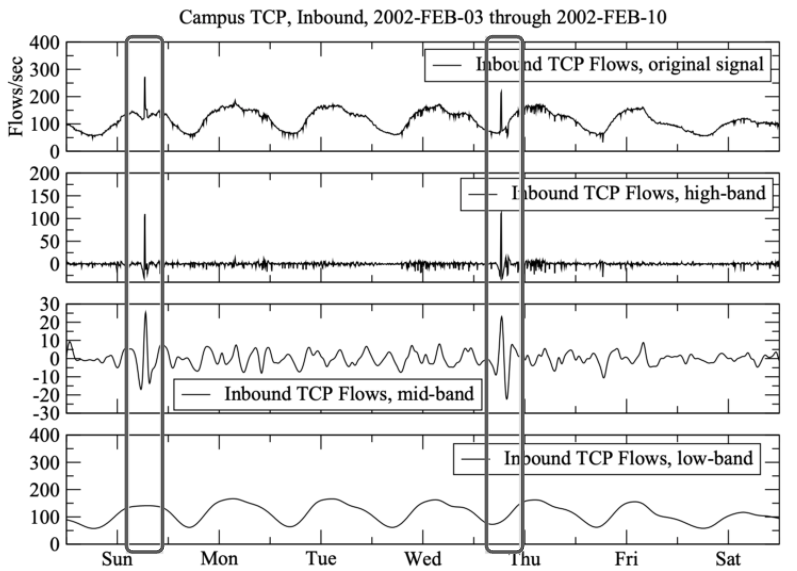
Figure 1: Example of packet flow signals for a one week period highlighting two anomalies plus high/mid/low decompositions.

Due to the mission-critical role of such work, this paper seeks ways to build anomaly detectors to specifically explore faulty Transmission Control Protocol (TCP) file transfers similar to those shown in grey boxes of Figure 1. According to Papadimitriou et al. [9], such anomalies represent a troubling class of problems. Several research works like [10, 11] have explored the use of Machine Learning (ML) to detect network anomalies. However, these existing works have mostly employed “off-the-shelf” ML models, e.g., scikit-learn, without exploring systematic hyperparameter tuning of the ML models themselves. Previous research on diverse Software Engineering (SE) problems have shown better learning can be achieved by tuning the control parameters of the ML tools [12, 7, 13, 14, 5]. Yet, tuning has its own limitations:

• A daunting number of options: Assuming that $R=25$ times we are analyzing $D$ data sets with say $L$ learners and $H$ hyperparameters with each $H$ has continuous or discrete $V$ values to pick, then with these settings, hyperparameter optimization with grid search needs to repeat the experiment millions of times ($R\times L\times D\times H\times V$). For instance, Table I is a sample of the options to explore in this space for $L,H,$ and $V$, which approximately reach billion of choices (assuming each numeric range divides into, say, 10 options). This is consistent with Agrawal et al.’s report [12].

• Slow convergence:  Fu et al. [15]’s replication work of Tantithamthavorn et al. [16] experiment requires 109 days of CPU. A worse case, decades of CPU time were needed by Treude et al. [17] to achieve a 12% improvement over the default settings.

• Poorly chosen default configuration: In ASE 2019’s Keynote speech, Zhou [18] remarked that 30% of errors in cloud environments are due to configuration errors.  Jamshidi and Casale [19] reported for text mining applications on Apache Storm, the throughput with the worst configuration is 480 times slower than the throughput achieved by the best configuration.

Recent work from the SE literature suggests that there exists better state-of-the-art (SOTA) methods to perform hyperparameter optimization with minimal computational cost [12, 7, 13, 14, 5]. In research on the DODGE($\epsilon$) algorithm,  Agrawal et al. [12] reported that with only 30 evaluations by navigating through the output (result) space of the sample of the learners, the preprocessors, and their corresponding parameter choices, DODGE($\epsilon$) outperforms traditional evolutionary approaches. In research on the FLASH algorithm, Nair et al. [20] reported that sequential model optimization method can be utilized for software configuration (and possibly hyperparameter tuning).

Drawing inspirations from these work. We designed a network anomaly detection method called X-FLASH, with (1) an ensemble model, XGBoost, and (2) FLASH as a sequential optimizer (to learn the optimal settings for the model). Overall, this paper makes the following contributions:

• Investigate the power of hyperparameter tuning to develop anomaly detectors for faulty TCP-based network transfer over SOTA off-the-shelf ML models.

• First to compare empirically the above two prominent SE-based approaches for hyperparameter tuning.

• Besides the performance improvement, tuning also changed the conclusion about the most important features for the anomaly detection.

As a service to other researchers, all the scripts and data of this study are available, on-line.

II Background

II-A Why Study Scientific Workflows?

Modern computational and data science often involve processing and analyzing vast amounts of data through large scale simulations of underlying science phenomena. With advantages in flexible representation to express complex applications with data and control dependencies, scientific workflows have become an essential component for data-intensive science. They have facilitated breakthroughs in several domains such as astronomy, physics, climate science, earthquake science, biology, among many others [21].

Reliable and efficient movement of large data sets is essential for achieving high performance in scientific workflow executions. Scientific workflow systems often leverage high-performance networks and networked systems to perform several kinds of data transfers for input data, output data and intermediate data. Hence, the performance and reliability of networks is key to achieving workflow performance. As the scientific workflows and the infrastructures supporting them keep increasing both in resource demands and complexity, there is an urgent need for the network to provide high throughput connectivity, in addition to being reliable, secure, and 99.9% available. However, there are bound to be anomalies in such large scale systems and applications. Such anomalies are particularly damaging for the scientific research community because (a) poor network performance (e.g., packet loss [11]) delays scientific discoveries, i.e., negatively impacts scientific productivity, and (b) data integrity issues arising from network errors [22] can jeopardize the validity of scientific results and the reputation of the researchers. Therefore, it is essential to identify and understand these network anomalies early on to allow the network administrator to respond to the anomalies and mitigate the problem.

II-B Anomaly Detection in Scientific Workflows

Scientific workflows can take a long time to complete execution because of their scale and complexity comprising a myriad of steps including data acquisition/transformation/pre-processing and model simulation/computing. Therefore, anomalies can be detrimental to both the scientists and the infrastructure providers in terms of lost productivity when long-running workflows fail. Various techniques could be used to predict and detect workflow anomalies. Although domain knowledge could be applied, e.g., “Execution $E_{i}$ has failed if it takes longer than $t$ seconds”, this approach is brittle and non-portable between applications and resource types.

Several existing works [23, 22, 24, 25, 26] in end-to-end monitoring of workflow applications and systems are essential building blocks to detect such problems. However, several techniques for anomaly detection are often based on thresholds and simple statistics (e.g., moving averages)  [27], which fail to understand longitudinal patterns, i.e., relationship between features. Hence, multivariate techniques based on ML are more appropriate to address the anomaly detection problem because they can capture the interactions and relationships between features, as recommended by Deelman et al. [28].

There is some existing research on the application of ML for scientific workflow anomaly detection. In 2013, Samak et al. [29] employed a Naive Bayes (NB) classifier to predict the failure probability of tasks for scientific workflows on the cloud using task performance data. They found that in some cases, a job destined for failure can potentially be executed successfully on a different resource. Others [30] have compared logistic regression, artificial neural nets (ANN), Random Forest (RF) and NB for failure prediction of cloud workflow tasks and found that the NB’s approach provided the maximum accuracy. In Buneci and Reed [31]’s work, the authors have used a k-nearest neighbors classifier to classify workflow tasks into “Expected” and “Unexpected” categories using feature vectors constructed from temporal signatures of task performance data. Recently, Dinal Herath et al. [25] developed RAMP, which is based on using an adaptive uncertainty function to dynamically adjust to avoid repetitive alarms while incorporating user feedback on repeated anomaly detection. In their previous work [32], they have presented a set of lightweight ML-based techniques, including both supervised and unsupervised algorithms, to identify anomalous workflow behaviors by doing workflow- and task-level analysis. However, none of the above ML-based approaches investigated the possibility of hyperparameter tuning.

II-C Model Optimization

All previous anomaly detection work in scientific workflow lack (1) model optimization and (2) a tuning study. Specifically, this paper is based on the work of Papadimitriou et al. [9] that applied solely off-the-shelf RF to study faulty TCP file transfers in scientific workflow. It is essential for this study to develop such anomaly detector with tuning as the backbone.

Many previous studies have advised that using data miners without parameter optimizer is not recommended [33, 5, 34] because: (1) such optimization can dramatically improve performance scores; and (2) any conclusions from unoptimized data miner can be changed by new results from the tuned algorithm. For example, Agrawal et al. [33] showed how optimizers can improve recall dramatically by more than 40%. Moreover, Fu et al. [5] showed how optimized data miners generate different features importance for software defect prediction task. Hence, it is necessary to use data miner using or used by optimizers. However, configuration in the analysis pipeline has numerous problems in their nature that are reported in the §I.

TABLE II: Top 10% important TCP Statistics features collected by the Tstat tool identified by the state-of-the-art model of [9] across the data. (S2C: Server to Client, C2S: Client to Server, Both: C2S and S2C)

Attribute	Types	Description
c_bytes_all	C2S	Number of bytes transmitted in the
		payload, including retransmissions
c_pkts_retx	C2S	Number of retransmitted segments
c_bytes_retx	C2S	Number of retransmitted bytes
s_ack_cnt_p	S2C	Number of segments with ACK field
		set to 1 and no data
durat	—	Flow duration since first to last packet
c/s_first	Both	Client/Server first segment with payload
		since the first flow segment
c/s_last	Both	Client/Server last segment with payload
		since the first flow segment
c/s_first_ack	Both	Client/Server first ACK segment (without
		SYN) since the first flow segment
c/s_rtt_avg	Both	Average RTT computed measuring the time
		elapsed between the data segment and
		the corresponding ACK
c/s_rtt_min	Both	Minimum RTT observed in connection lifetime
c/s_rtt_max	Both	Maximum RTT observed in connection lifetime

Solving these configurations is not limited to software systems and hyperparameter optimization in ML but also for cloud computing and software security. In cloud computing, different analytic jobs have diverse behaviors and resource requirements, choosing the correct combination of virtual machine type and cloud environment can be critical to optimize the performance of a system while minimizing cost [35, 36, 37, 38, 39]. In security of cloud computing, such problems of how to maximize conversions on landing pages or click-through rates on search-engine result pages [40, 41, 42] has gathered interest.

II-D Faulty TCP Case Study

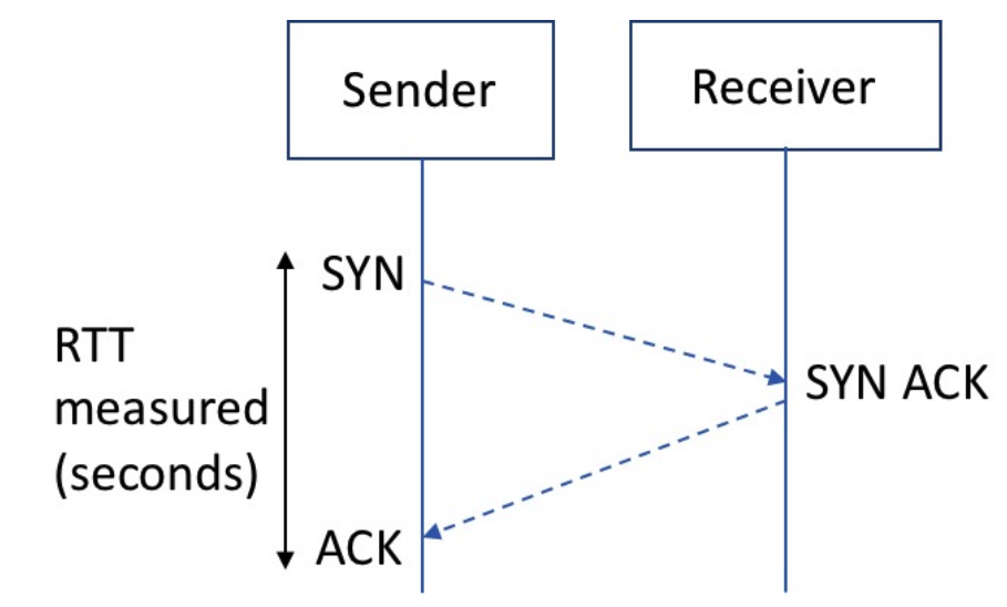
Figure 2: Round Trip Time measured in TCP’s three way communication.

In this work, we analyze anomalous network transfers by utilizing data collected using TCP statistics (Tstat) [43], which is a tool to collect TCP traces for transfers. How TCP works can be demonstrated in Figure 2 as follows: the server sends a packet to a client (with the load in bytes), when the client receives the packet, it sends an “acknowledgment” (ACK) signal back. The round trip time (RTT) is the total time from sending the package to receiving the ACK. Time windows is a measure that is used by the TCP protocol to allow servers to wait for the ACK, before deciding to resend the packet again.

Other than package loss, there is significant effort to recognize overflowing buffers [44, 45] and commonly occurring network anomalies seriously impact user experience and also affecting the clients’ work negatively as mentioned in §II.A. Described by [46, 47, 48], three common network anomalies targeted by this study are:

• Packet Loss happens when one or more packets fail to reach their destination. These could either be caused by errors in transmission or too much congestion on link, causing routers to randomly drop packets.

• Packet Duplication happens when the sender re- transmits packets, thinking that the previous packets have not reached their destination. This can be commonly observed when packet losses happen and retransmits increase.

• Packet Reordering happens when arrival order of packets or sequence number is completely out-of- order. In the case of real-time media streaming application, it is particularly relevant to show network instability.

Collectively, Tstat traces contain 133 variables per packet on both server and client sides so TCP protocol can ensure the packages are delivered reliably. These features are listed in details on Tstat’s documentation . Table II reports the top 10% features ranked by their importance shared across the data by applying the state-of-the-art work by Papadimitriou et al. [9]. It is mission-critical to understand what attributes are essential to the model to make decisions on classifying the right type of anomalies. Yet, the tuning study here showed that the important attributes reported before tuning and after tuning change significantly. This indicates that previous anomalies detection work reported misleading key features to the system managers or scientists which can cost them extra resource to debug. Accordingly, our proposed solution, X-FLASH does inform the right key features to the system experts to take appropriate action and prevent future network anomalies.

TCP provides reliable and error-checked delivery of a data stream between senders and receivers. Research efforts have been focusing on TCP extensions as variants to allow improvement of various network anomalies and enable congestion control. Jacobson et al. [49] established implementations of the modern TCP. Since that seminal work, some TCP variants are introduced to prioritize throughput over loss prevention. In this paper scope, we specifically focus on four of these variants: Cubic, Reno, Hamilton, and BBR. For more information regarding these variants, please see [9].

III Software Configuration Optimization

The case was made above that (a) anomalies detection in scientific workflow is mission-critical, (b) previous studies lack optimization for their analytics pipelinem, and (c) tuning is a daunting task that requires careful attention per domain. Therefore, X-FLASH is designed to include tuning in the data mining pipeline for anomalies detection in scientific workflow. This section described how FLASH and DODGE($\epsilon$) can tune the data mining pipeline for a better scientific workflow anomalies detection.

III-A Core Problem

The problem can be described starting with a configurable data miner has a set $X$ of configurations $x\in X$. Let $x_{i}$ represent the $ith$ configuration of a data miner method. $x_{i,j}$ represent the $jth$ configuration option of the configuration $x_{i}$. In general, $x_{i,j}$ indicates either an (i) integer variable or a (ii) Boolean variable. The configuration space (X) represents all the valid configurations of a data miner tool. The configurations are also referred to as independent variables ($x_{i}$) where $1\leq i\leq|X|$, has one (single-objective) corresponding performance measures $y_{i,k}\in Y$ indicating the $1\leq kth\leq m$ objective (dependent variable). In our setting, the cost of optimization technique is the total number of iteration required to find the best configuration settings.

We consider the problem of finding a good configuration, $x^{*}$, such that $f(x^{*})$ is less than other configurations in X. Our objective is to find $x^{*}$ while minimizing the number of iterations and measurements.

III-B Overview

The heart of this problem is to optimize the analytical results (performance) with the knowledge at hand while minimizing the iterations (time) for the model to converge. In SE literature, the solution can be seen with evolutionary optimization (based on mutating existing configurations). However, according to Nair et al. [20] and Agrawal et al. [6, 7, 12], such optimization can be cost inefficient, slow convergence, and poor performance. Hence, research in software configuration in the last decade has explored non-EA methods including Sequential Model-Based optimization, and $\epsilon$-dominance.

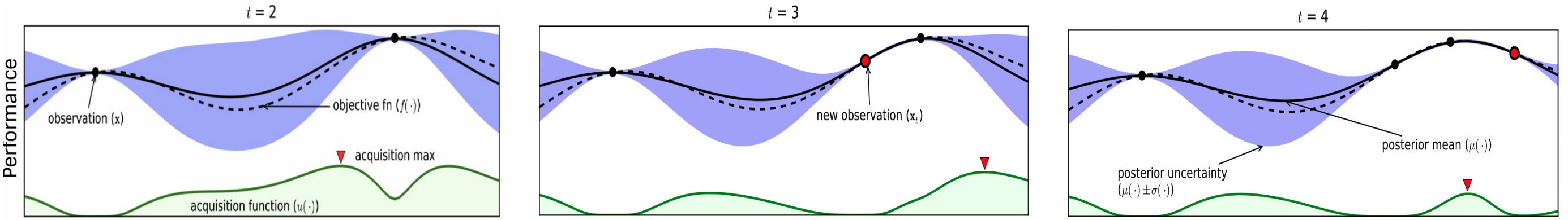
Figure 3: An example of Sequential Model-based method’s working process from Brochu et al. [50]. The figures show a Gaussian process model (GPM) of an objective function over four iterations of sampled values. Green shaded plots represent acquisition function. The value of the acquisition function is high where the GPM predicts larger objective and where the prediction uncertainty (confidence) is high such points (configurations in our case) is sampled first. Note that the area on the far left is never sampled even when it has high uncertainty (low confidence) associated.

For those reasons, research in this area in the last decade has explored non-EA methods for software configuration.

III-B1 Sequential Model-Based optimization

FLASH is a variant of Sequential Model-based Optimization (SMBO) whose core concept is “given what we know about the problem, what should we do next?”. To illustrate this, consider Figure 3 of SMBO. The bold black line represents the actual performance function ($f$, which is unknown in our setting) and the dotted black line represents the estimated objective function (in the language of SMBO, this is the prior). The optimization starts with two points (t=2). At each iteration, the acquisition function is maximized to determine where to sample next. A model is built on the points and these evaluated measurements as the prior belief. This model can then learn where to sample next and find extremes of an unknown objectives. A posterior is then defined and captured as our updated belief in the objective function or surrogate model. The purple regions represent the configuration or uncertainty of estimation in a region—the thicker that region, the higher the uncertainty. The green line in that figure represents the acquisition function. The acquisition function is a user-defined strategy, which takes into account the estimated performance measures (mean and variance) associated with each configuration. The chosen sample (or configuration) maximizes the acquisition function ($argmax$). This process terminates when a predefined stopping condition is reached which is related to the budget associated with the optimization process.

Gaussian process models are often the surrogate model of choice in the literature. Yet, building GPM can be very challenging since (1) GPM can be very fragile to the parameters setting and (2) GPM do not scale to high dimensional data as well as large data set (i.e., large option space). Therefore, Nair et al. [20] proposed the SMBO’s improvement, i.e., FLASH:

• FLASH models each objective as a separate Classification and Regression Tree (CART) model. Nair et al. reported that the CART algorithm can scale much better than other model constructors (e.g., Gaussian Process Models).

• FLASH replaces the actual evaluation of all combinations of parameters(which can be very slow) with a surrogate evaluation, where the CART decision trees are used to guess the objective scores (which is very fast). Such guesses may be inaccurate but, as shown by Nair et al. [20], such guesses can rank guesses in (approximately) the same order as that generated by other, much slower, methods [51].

FLASH can be executed as follow:

1. Initial Sampling: A sample of predefined configurations from the option space is evaluated. The evaluated configurations are removed from the unevaluated pool.

2. Surrogate Modeling: The evaluated configurations and the corresponding performance measures are then used to build CART models.

3. Acquisition Modeling: The acquisition function accepts the generated surrogate model (or models) and the pool of unevaluated configurations (uneval configs) to choose the next configuration to measure.

   For multi-objective problems, for each configuration $x_{i}$, $N$ (random projections) vectors $V$ of length $o$ (objectives) are generated with:

   • Guess it’s performance score $y_{i,j}$ using CART.

   • Compute its mean weight as:

     $mean_{i}=\frac{1}{N}\sum_{n}^{N}\sum_{j}^{o}(V_{n,j}\cdot y_{i,j})$

   • if $mean_{i}>max_{current}$ then $best=x_{i}$.

4. Evaluating: The configuration chosen by the acquisition function is evaluated and removed from the configuration candidates pool.

5. Terminating: The method terminates once it runs out of a predefined budget.

FLASH was invented for the software configuration problem as it performed faster than more traditional optimizers such as Differential Evolution [52] or NSGA-II [53]. FLASH is an improvement of SMBO and was chosen as the optimizer component for X-FLASH in a few technical areas including:

• For surrogate modeling, CART is replaced with GPM. GPM would have taken $O(M^{3})$ time whereas CART is a bifurcating algorithm that would only take $O(M\cdot N^{2})$ where M is the size of the training dataset and N is the number of attributes.

• FLASH’s acquisition function uses Maximum Mean. By assuming that the greatest mean might contain the values that most extend to the desired maximal (or minimal) goals. It cut the runtime from $O(M^{2})$ to only $O(M)$.

• GPM assumed smoothness where configurations that are close to each other have similar performance. However, CART makes no assumption that neighboring regions have the same properties.

III-B2 DODGE and $\epsilon$-Dominance

In 2005, Deb et al. [54] proposed partitioning the output space of an optimizer into $\epsilon$-sized grids. In multi-objective optimization (MOO), a solution is said to dominate the other solutions if and only if it is better in at least one objective, and no worse in other objectives. A set of optimal solutions that are not dominated by any other feasible solutions form the Pareto frontier. Figure 4 is an example of the output space based on $\epsilon$-dominance. The yellow dots in the figure form the Pareto frontier.

Deb’s principle of $\epsilon$-dominance is that if there exists some $\epsilon$ value below which is useless or impossible to distinguish results, then it is superfluous to explore anything less than $\epsilon$ [54]. Specifically, consider distinguishing the type of anomalies discussed in this paper, if the performances of two learners (or a learner with various parameters) differ in less than some $\epsilon$ value, then we cannot statistically distinguish them. For the learners which do not significantly improve the performance, we can further reduce the attention on them.

Agrawal et al. [12] successfully applied $\epsilon$-dominance to some SE tasks such as software defect prediction and SE text mining. Their proposed approach, named DODGE($\epsilon$), was a tabu search, i.e., if some settings arrive within $\epsilon$ of any older result, then DODGE($\epsilon$) marked that option as “to be avoided”.

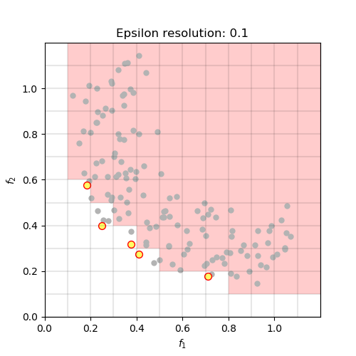
Figure 4: An example of Pareto frontier [55]. Objectives $f_{1}$ and $f_{2}$ are both to be minimized. $\epsilon$ value is set to 0.1. The gray dots represent the feasible solutions. The yellow dots represent the Pareto optimal solutions.

A tool for software analytics, DODGE($\epsilon$) needed just a few dozen evaluations to explore billions of configuration options for (a) choice of learner, for (b) choice of pre-processor, and for (c) control parameters for the learner and pre-processor. These configurations, when combined together, make up billions of options that are reported in Table 1 of [12]. DODGE($\epsilon$) executed by:

1. Assign weights $w=0$ to configuration options.

2. $N=30$ times repeat:

   1. Randomly pick options, favoring those with most weight;

   2. Configuring and executing data pre-processors and learners using those options;

   3. Dividing output scores into regions of size $\epsilon=0.2$;

   4. if some new configuration has scores with $\epsilon$ of prior configurations then…

      • …reduce the weight of those configuration options $w=w-1$;

      • Else, add to their weight with $w=w+1$.

3. Return the best option found in the above.

Note that after Step 2d, the choices made in subsequent Step 2a will avoid options that result in $\epsilon$ of other observed scores.

Experiments with DODGE($\epsilon$) found that best learner performance plateau after just $N=30$ repeats of Steps 2-5. To explain this result, [12] note that for a range of software analytics tasks, the outputs of a learner divide into only a handful of equivalent regions. For example, when a software analytics task is repeated 10 times, each time with 90% of the data, then the observed performance scores (e.g., recall, false alarm) can vary by 5 percent, or more. Assuming normality, then scores less than $\epsilon=1.96*2*0.05=0.196$ are statistically indistinguishable. Hence, for learners evaluated on (say) $N=2$ scores, those scores effectively divide into just $C=\left(\frac{1}{\epsilon=0.196}\right)^{N=2}=26$ different regions. Hence, it is hardly surprising that a few dozen repeats of Steps 2-5 were enough to explore a seemingly very large space of options.

IV Methodologies

While the above DODGE($\epsilon$) and FLASH algorithms have been shown to work well for analytics tasks in software engineering (e.g., effort estimation, bug location etc). These algorithms have not been successfully deployed outside the realm of SE. Accordingly, the rest of this paper tests if DODGE($\epsilon$) and/or FLASH work well for anomaly detection for faulty Transmission Control Protocol.

IV-A Data

The data here is adopted from the SOTA TCP anomaly detection [9]. It includes two sets of datasets of Mice&Elephant Flows and 1000 Genome Workflow where each set include four datasets corresponding to four TCP variants (Hamilton, BBR, Reno, and Cubic) under normal or anomalous conditions (loss, duplicate, and reordering). A summary of both sets is captured in Table III which depicts the number of collected flows across anomaly types and TCP variants.

IV-A1 Mice and Elephant Flows

ExoGENI testbed [3] is used to generate this labeled set of data. ExoGENI is a federated cloud testbed designed for experimentation and computational tasks. It is orchestrated over a set of independent cloud sites located across US and connected via national research circuit providers through their programmable exchange points. Mice flows were aimed for 1000 SFTP transfers with a transfer size between 80 MB and 120 MB, the link bandwidth is set to 1 Gbps among all the nodes. Elephant flows were aimed for 300 SFTP transfers with a transfer size between 1 and 1.2 GB, the link bandwidth is set to 100 Mbps among all the nodes.

TABLE III: Number of flows generated at Data Node across TCP variants (H-Hamilton, B-BBR, R-Reno, & C-Cubic) under normal or anomalous settings (loss, duplicate, & reordering) for Mice&Elephant Flows and 1000 Genome Workflow.

	Mice&Elephant Flows				1000 Genome Workflow
Type	H	B	R	C	H	B	R	C
Normal	1304	1304	1304	1304	550	508	532	528
Loss	3994	3975	3989	3995	6110	10588	1212	1721
Duplicate	2616	2615	2616	3778	1111	1016	1097	1083
Reordering	3830	2612	2612	2614	1141	1019	1078	1067

IV-A2 1000 Genome Workflow Transfers

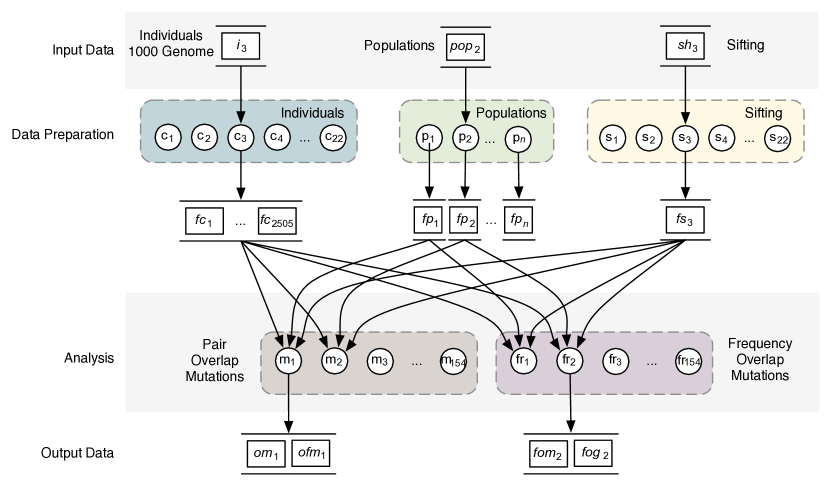
Figure 5: The overview of 1000 Genome sequencing analysis workflow.

The data used in this study are comprised of network traces produced by the 1000 Genome Pegasus workflow. This science workflow is inspired by the 1000 genomes project which provides a reference for human variation, having reconstructed the genomes of 2,504 individuals across 26 different populations [56]. The version of the 1000 Genome workflow used (Figure 5) is composed of five different tasks: (1) individuals – fetches and parses the Phase 3 data from the 1000 genomes project per chromosome; (2) populations – fetches and parses five super populations (African, Mixed American, East Asian, European, and South Asian) and a set of all individuals; (3) sifting – computes the SIFT scores of all of the SNPs (single nucleotide polymorphisms) variants, as computed by the Variant Effect Predictor; (4) pair overlap mutations – measures the overlap in mutations (SNPs) among pairs of individuals; and (5) frequency overlap mutations – calculates the frequency of overlapping mutations across subsamples of certain individuals. During the lifetime of the workflow, most of the data needs to be staged in during the first part of the workflow (individuals) with many smaller transfers following to accommodate the execution of the rest of the processing tasks. In their experiments, they included a comprehensive list of TCP and conducted workflow transfers under normal and various anomalous conditions in II-D.

IV-B Data Miners

Hyperparameter optimizers (i.e., FLASH) tune the settings of data miners. This section describes such data miner candidates to be tuned in this study.

IV-B1 CART and RF

We use CART to recursively build decision trees to find the features that reduce most of entropy, where a higher entropy indicates less ability to draw conclusion from the data being processed [57]. Using CART as a sub-routine, our Random Forest method builds many trees, each time with different subsets of the data rows $R$ and columns $C$. Test data is then passed across all $N$ trees and the conclusions are determined (say) a majority vote across all the trees [58]. Holistically, RF is based on bagging (bootstrap aggregation) which averages the results over many decision trees from sub-samples (reducing variance). Both are popular in the field of ML and implemented in popular open-source toolkit Scikit-learn by [8].

We choose to use CART for its explainability and efficiency, as discussed in [20, 59, 34]. RF was used in the previous study for this same problem for its advantages of performance [60]. However, we will show later in this paper that RF without optimization is not enough.

IV-B2 XGBoost

Gradient Boosting is chosen as a model for it’s advantages of reducing both variance and bias. It is an ensemble model which involves:

• Boosting builds models from individual so called “weak learners” in an iterative way. The individual models here are not built on completely random subsets of data and features but sequentially by putting more weight on instances with wrong predictions and high errors (reducing biases).

• The gradient is a partial derivative of our loss function - so it describes the steepness of our error function in order to minimize error in the next iteration.

Gradient Boosting reduces the variances with multiple models (similar to bagging in RF) and also reduces bias with subsequently learning from previous step (boosting). XGBoost is an improved Gradient Boosting method by (1) computing second-order gradients, i.e., second partial derivatives of the loss function (instead of using CART as the loss function); and (2) advanced regularization (L1 & L2) [61].

IV-C Evaluation Metrics

The problem studied in this paper is a multiclass classification task with four classes (1 normal class and 3 anomalous classes). The performance of such multiclass classifier can be assessed via a confusion matrix as shown in Table IV where each class is denoted as $C_{i}$.

Further, “false” means the learner got it wrong and “true” means the learner correctly identified a positive or negative class. The four counts include True Positives (TP), False Positive (FP), False Negative (FN) and True Negative (TN).

TABLE IV: Results Matrix of Multiclass Classification

	Actual
Prediction	C1	C2	C3	C4
C1	$\mathit{TP_{11}}$	$\mathit{FN_{12}}$	$\mathit{FN_{13}}$	$\mathit{FN_{14}}$
C2	$\mathit{FP_{21}}$	$\mathit{TP_{22}}$	$\mathit{FN_{23}}$	$\mathit{FN_{24}}$
C3	$\mathit{FP_{31}}$	$\mathit{FP_{32}}$	$\mathit{TP_{33}}$	$\mathit{FN_{34}}$
C4	$\mathit{FP_{41}}$	$\mathit{FP_{42}}$	$\mathit{FP_{43}}$	$\mathit{TP_{44}}$

Due to the multiclass and anomalies detection nature with no imbalanced class issue observed, we want to make sure all classes are treated fairly. A macro-average is preferred to compute each metric independently for each class $C_{i}$ and then take the average. Ling et al. [62] and Menzies et al. [63] had warned us against accuracy and precision as evaluation metrics even when the original work employed accuracy. Therefore, we used 3 macro-average measures, i.e., recall, F-measure (a harmonic mean of precision and recall), and G-score (a harmonic mean of recall and false-alarm rate, or FAR) to evaluate the learners that are calculated as below:

• $Precision=\frac{\sum_{i=1}^{L}\frac{TP_{i}}{TP_{i}+FP_{i}}}{L}$

• $FAR=\frac{\sum_{i=1}^{L}\frac{FP_{i}}{TP_{i}+TN_{i}}}{L}$

$$\scriptsize Recall=\frac{\sum_{i=1}^{L}\frac{TP_{i}}{TP_{i}+FN_{i}}}{L}$$ (1)

$$\scriptsize F-measure=\frac{2*Precision*Recall}{Precision+Recall}$$ (2)

$$\scriptsize\mathit{G-score}=\frac{2\cdot\mathit{Recall}\cdot\mathit{(1-FAR)}}{\mathit{Recall}+(1-\mathit{FAR})}$$ (3)

IV-D Statistical Testing

We compared our results using Scott-Knott method, which sorts results from different treatments, and then splits them to maximize the expected value of differences in the observed performances before and after divisions. For lists $l,m,n$ of size $\mathit{ls},\mathit{ms},\mathit{ns}$ where $l=m\cup n$, the “best” division maximizes $E(\Delta)$; i.e., the delta in the expected mean value before and after the split:

$$E(\Delta)=\frac{ms}{ls}abs(m.\mu-l.\mu)^{2}+\frac{ns}{ls}abs(n.\mu-l.\mu)^{2}$$

Scott-Knott then checks if that “best” division is actually useful. To implement that check, Scott-Knott would apply some statistical hypothesis test $H$ to check if $m,n$ are significantly different (and if so, Scott-Knott then recurses on each half of the “best” division). For this study, our hypothesis test $H$ was a conjunction of statistical significance test and an effect size test. Specifically, significance test here is non-parametric bootstrap sampling, which is useful for detecting if two populations differ merely by random noise, cliff’s delta [64, 4]. Cliff’s delta quantifies the number of difference between two lists of observations beyond p-values interpolation [65]. The division passes the hypothesis test if it is not a “small” effect ($Delta\geq 0.147$). The cliff’s delta non-parametric effect size test explores two lists $A$ and $B$ with size $|A|$ and $|B|$:

$$Delta=\frac{\sum\limits_{x\in A}\sum\limits_{y\in B}\left\{\begin{array}[]{l}+1,\mbox{ if $x>y$}\\ -1,\mbox{ if $x<y$}\\ 0,\mbox{ if $x=y$}\end{array}\right.}{|A||B|}$$ (4)

In this expression, cliff’s delta estimates the probability that a value in list $A$ is greater than a value in list $B$, minus the reverse probability [65]. This hypothesis test and its effect size is supported by Hess and Kromery [66].

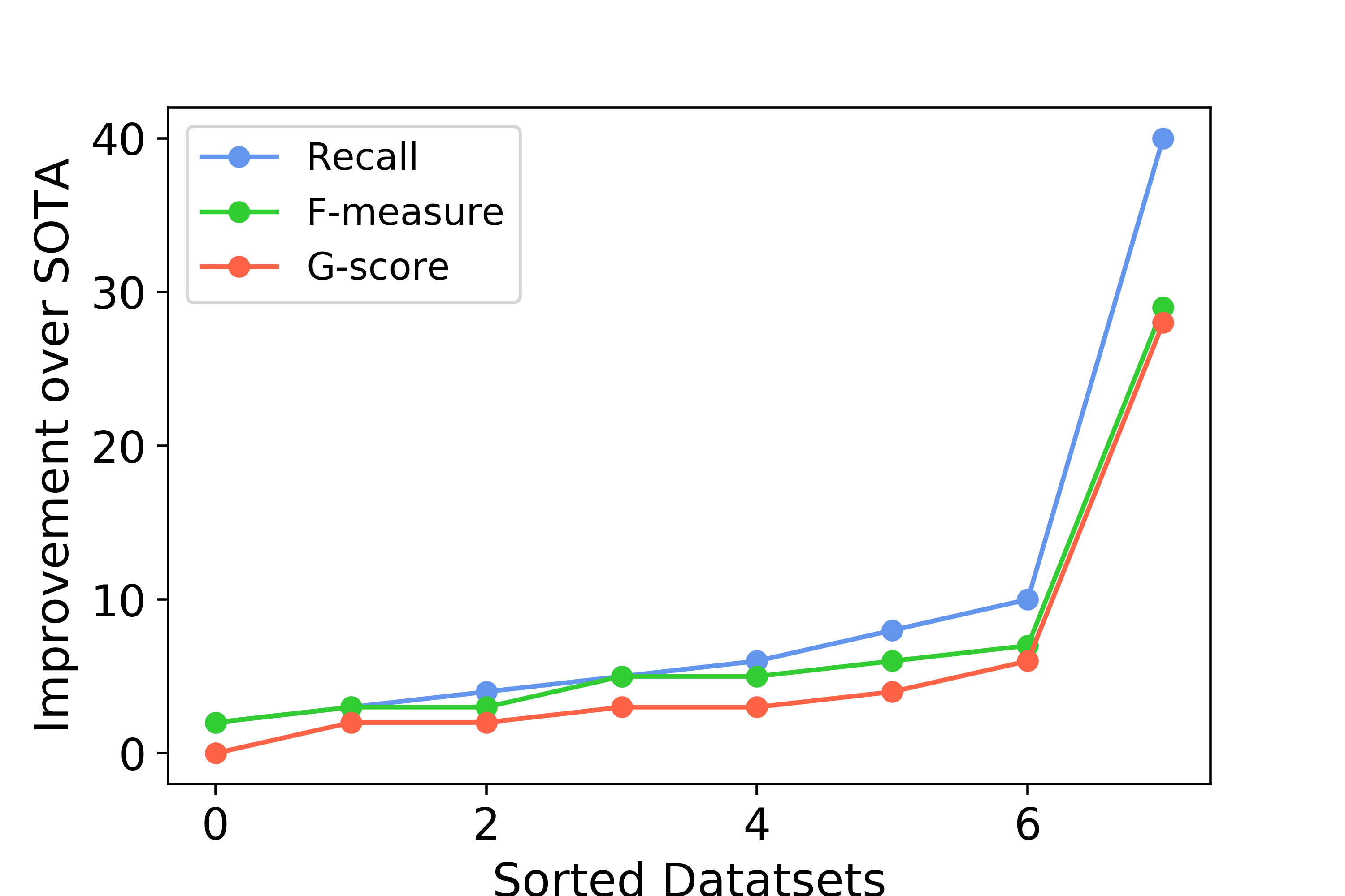
Figure 6: Sorted relative median delta for each performance across all datasets between X-FLASH and RF (SOTA work’s choice of data miner method).

IV-E Test Rig

We applied $k$-fold cross-validation, with $k=10$ to randomly partition the data into k equal sized subsamples. A single subsample among them is retained for testing, and the remaining $k-1$ subsamples are used for tuning and validation with the proportions of 80% and 20% respectively. FLASH and DODGE($\epsilon$) are applied on tuning dataset and validated on validation dataset before evaluated on the test dataset. The cross-validation process is then repeated $k$ times. The advantage of this method over repeated random sub-sampling is that all observations are used for both training and testing.

TABLE V: Default and median tuned configurations of four XGBOOST’s parameters when tuning for a specific metric (recall, F-measure, and G-score) across eight datasets.

Parameter	Defaut	Recall	F-measure	G-score
max_depth	3	12	17	19
learning_rate	0.1	0.53	0.53	0.58
#_estimators	100	107	105	106
booster	gbtree	dart	gbtree	dart

V Results

TABLE VI: Recall, F-measure, and G-score (higher the better) results are reported between all the methods that are ranked by Scott-Knott statistical tests. Medians and IQRs (delta between 75th percentile and 25th percentile, lower the better) are calculated for easy comparisons. The best performing one is noted as a gray cell for each metric per column. The column #Best shows the number of projects each treatment performs the best in.

Metrics	Treatment	Mice and Elephant Flows				1000 Genome Workflow				Median	IQR	#BEST
		HAMILTON	BBR	RENO	CUBIC	HAMILTON	BBR	RENO	CUBIC
Recall	X-FLASH	84	50	89	70	85	92	73	95	85	17	8
	FLASH_CART	81	49	84	68	71	82	66	87	76	15	2
	FLASH_RF	80	49	84	68	78	85	52	91	79	20	2
	DODGE	78	48	85	68	70	81	63	86	74	15	1
	CART	81	49	84	68	72	82	67	87	77	14	2
	RF	80	49	84	68	77	85	52	91	79	20	2
	XGBOOST	71	39	74	58	69	81	39	89	70	22	0
F-measure	X-FLASH	83	49	88	71	86	91	80	94	85	11	8
	FLASH_CART	81	48	85	69	70	80	67	87	75	13	2
	FLASH_RF	79	49	84	69	80	85	62	92	80	17	2
	DODGE	77	48	85	68	70	80	63	85	74	14	2
	CART	81	49	84	69	73	82	67	86	77	14	2
	RF	79	49	84	69	81	85	62	91	80	17	2
	XGBOOST	72	36	75	56	73	82	45	90	73	23	0
G-score	X-FLASH	88	62	92	80	90	94	83	96	89	10	8
	FLASH_CART	86	62	89	78	78	87	78	91	82	9	2
	FLASH_RF	86	62	89	78	85	89	64	94	86	14	2
	DODGE	85	61	90	78	79	87	73	91	82	11	1
	CART	87	62	90	78	81	87	77	91	84	10	2
	RF	86	62	89	78	85	90	65	94	86	14	2
	XGBOOST	80	52	83	70	79	88	52	93	80	18	0

RQ1: Does tuning improve the performance of anomalies detection?

For our first set of results, default learners (RF and CART and XGBOOST) are compared with data miners with optimization (FLASH and DODGE ($\epsilon$)).

Table VI shows those results, including the statistical ranking generated from Scott-Knott test in §IV.D for recall, F-measure, and G-score metrics defined in §IV.C. Across all 8 datasets (HAMILTON, BBR, RENO, and CUBIC for 1000 Genome Workflow and Mice&Elephant Flows), X-FLASH performed the best. Improvement with the previous work can be observed closely in Figure 6. X-FLASH improved up to 28%, 29%, and 40% relatively for F-measure, G-score, and recall respectively. The benefit of tuning is even higher when comparing between XGBOOST and X-FLASH. In one extreme case, it improved 45%, 52%, & 39% to 80%, 83,%, & 74% respectively for F-measure, G-score, and recall (which are 60%, 78%, and 87% relative improvement). This is explainable as shown in Table V. Except the number of estimators parameter (n_estimators), the other three parameters values, when tuned, are far away from the default values. This shows that the default configurations for a data miner are not one-size-fits-all across different datasets and domains, hence, should be deprecated. With a mission-critical task like anomalies detection, it is essential to optimize the solution at hand specific for the domain, dataset, and metric.

Moreover, X-FLASH notably outperformed DODGE($\epsilon$), where DODGE($\epsilon$) is a state-of-the-art data mining with optimization method taken from Software Engineering literature [12] (bug reports classification, close-issues prediction, defect prediction, etc). This shows that a method that works well for one disciplinary field may not work well in a different field. It is critical that the scientists and researchers revise and tune the method based on the specific conditions.

TABLE VII: Sorted time performance (in seconds) on median for the studied data mining methods on eight datasets, across TCP variants (H-Hamilton, B-BBR, R-Reno, and C-Cubic) for Mice&Elephant Flows and 1000 Genome Workflow.

	Mice&Elephant Flows				1000 Genome Workflow
Type	H	B	R	C	H	B	R	C
XGBOOST	6	5	5	5	16	4	15	4
DODGE($\epsilon$)	130	167	173	272	63	24	154	32
X-FLASH	628	400	437	563	453	139	617	165

RQ2: Is tuning anomalies detection impractically slow?

To our surprise, X-FLASH achieved statistically significant improvement in the performance scores for our data miners in less than 30 evaluations. In this space, our proposed solution took the most time among default and the state-of-the-art optimizer DODGE($\epsilon$) (30 evaluations). However, considering the mission-critical nature of the problem and it still take less than 11 minutes at most with standard hardware (i.e., CPU) from Table VII. The performance increments seen in Figure 6 and Table VI are more than to compensate for the extra CPU required for X-FLASH. Modern hardware choices (e.g., GPUs) and parallel computation can be configured to improve the time to be more practical for the industry.

TABLE VIII: Non-overlapped Features selected by default XGBOOST versus after tuned by FLASH across TCP variants (H-Hamilton, B-BBR, R-Reno, and C-Cubic) for Mice&Elephant Flows and 1000 Genome Workflow.

Datasets		DEFAULT	Tuned by FLASH
Mice	H	s_rtt_avg, s_ack_cnt_p	c_ttl_min, s_rtt_min
&	B	c_bytes_uniq, s_rtt_avg	c_fin_cnt, c_first_ack
Elephant	R	s_ack_cnt_p	c_ttl_min
Flows	C	s_rtt_avg, s_ack_cnt_p	c_first_ack, s_rtt_max
	H	s_last_handshakeT, c_rtt_std,	s_pkts_retx, s_pkts_data,
		c_pkts_unfs, c_ack_cnt_p	s_fin_cnt, s_rtt_cnt
	B	c_appdataT, s_first_ack,	c_pkts_reor, c_bytes_retx,
1000		s_win_max, s_rtt_std	c_win_max, c_pkts_fs
Genome	R	c_bytes_retx, c_first_ack	c_pkts_rto, c_pkts_retx,
Work-		s_first_ack, c_mss_max	c_pkts_ooo, s_win_min,
Flow		s_win_max, c_appdataT	c_pkts_unk, c_cwin_max
	C	c_pkts_rto, c_cwin_max,	c_pkts_fs, s_cwin_min,
		s_rtt_min, c_appdataT,	c_pkts_unfs, c_bytes_retx
		s_ack_cnt_p	c_ack_cnt_p

RQ3: Does tuning change conclusions about what factors are most important in anomalies detection?

It is important to understand which attribute(s) associated more with differentiating characteristics between different types of anomalies and normal scientific flows. Scientists and network managers can then inspect the flagged ones with high likelihood of anomalies. From Table VIII, among the top ten important features (curated from the built-in feature_importances_ function [67]), the median number of features is seven as commonly chosen decisive factors for the anomalies detectors (while the rest 30% of top ten features are not the same, non-overlapped features). It demonstrated how the previous study [9] and conclusion from default learner can be untrustworthy. They did not attempt to do the features importance analysis of their anomaly detectors.

Interestingly, the learners rankings were also changed slightly with tuning. Default CART model performed similarly or better than default XGBoost in 7 out of 8 datasets across recall, F-measure, and G-score respectively. However, after tuning through FLASH, XGBoost always better across 8 datasets for each metric.

VI Discussions

In this section, we discuss the possible factors that affect the effectiveness of evaluations. Such factors also commonly exist in other research works with large scale empirical studies.

VI-A Evaluation Bias

This paper employed recall, F-measure, and G-score to evaluate the overall performance. We have taken into generalization issues of single metrics (e.g., accuracy and precision) into consideration and instead evaluate our methods on metrics that aggregate multiple metrics like F-measure and G-score. As the future work, we plan to test the proposed methods with additional analysis that are endorsed within SE literature (e.g., P-opt20 [68]) or general ML literature (e.g., MCC [69]).

For result validity, we applied bootstrap significant test and the cliff-delta effect size test. Hence, in this paper, “X was different from Y” conclusions were based on both tests.

VI-B Learner Bias

This work proposed X-FLASH (XGBoost + FLASH) data mining method and compared it with DODGE ($\epsilon$), endorsed by the SE literature. As the future work, we plan to test if the conclusions (data miner + optimization, called X-FLASH, is a good way to detect and classify anomalies) hold across multiple tasks associated with scientific workflows.

VI-C Sampling Bias

As a common issue for data mining field, our work is subject to possible sampling bias, i.e., the conclusion for the data we studied in this paper may not hold for other types of data. To ensure data and code availability for the research community, we release our code and data at https://github.com/msr2021/tuningworkflow/.

VI-D External Validity

The approach, DODGE($\epsilon$), that SE literature have established as “standard tool” may not be “general” to all the fields. Rather, the tools that are powerful in their home domain may need to be used with caution, if applied to new domains such as scientific workflow (and specifically, anomalies detection). Some of the data quirks that essential to the success of DODGE($\epsilon$) include: (1) the prediction is binary (e.g., 0 or 1, faulty or non-faulty, etc); and (2) the target class is infrequent. Those data quirks may lead to issues such as:

• It is harder to find the target;

• The larger the observed $\epsilon$ in the results;

• The greater the number of redundant tunings;

Therefore, since software engineering often deals with relatively infrequent target classes, we should expect to see a large $\epsilon$ uncertainty in our conclusion which is more likely that DODGE($\epsilon$) will work. However, for the faulty TCP file transfers detection in this paper, it is a multiclass classification and the distribution is only infrequent for the normal flows instead of the targets (i.e., anomalies flows). Therefore, for such a more dynamic problem with multiple target classes and the distribution is diverse, FLASH is recommended as a more general approach for optimization.

In summary, and in support of the general theme of this paper, this external validity demonstrates the danger of treating all data with the state-of-the-art method, especially when switching domain (e.g., DODGE($\epsilon$) from SE literature).

VII Conclusion

In this paper, we show that utilizing general anomalies learning tools for faulty TCP file transfers without tuning can be considered harmful and misleading to the reliability of networked infrastructures. Our proposed solution X-FLASH combined an ensemble model (XGBoost) and a sequential model-based optimizer (FLASH) from Software Engineering literature to detect and classify the correct malicious activity or attacks, before it contaminates downstream scientific process:

• Tuning default learners will improve the relative performance up to 28%, 29%, and 40% for F-measure, G-score, and recall (see Table VI) from the SOTA work [9].

• Tuning changes previous conclusions on what learner is the best performing, i.e., from RF to XGBoost.

• Tuning changes previous conclusions on what factors are most influential in detecting for anomalies by 30% (see Table VIII).

Moreover, results showed that X-FLASH out-performed state-of-the-art data mining in SE literature, DODGE($\epsilon$) by  Agrawal et al. [12]. This result is suggestive (but not conclusive) evidence that (a) prior work on analytics has over-fitted methods (to systems like Apache); and that (b) there is no better time than now to develop new case studies (like scientific workflows).

As to future work, it is now important to explore the implications of these conclusions to other kinds of scientific workflow analytics. Specifically, previous papers for anomalies detection for scientific workflow [23, 22, 24, 25, 26, 25, 31, 30, 29] that not based on TCP data transfers should be also reinvestigated as none have done tuning study to avoid falling in the same retracted category.

VIII Acknowledgements

We thank the Computational Science community from the Pegasus Research group and Renaissance Computing Institute at UNC (RENCI) for their assistance with this work.

This work was partially funded by an NSF CISE Grant #1826574, #1931425 and DOE contract number #DE- SC0012636M, “Panorama 360: Performance Data Capture and Analysis for End-to-end Scientific Workflows”.

References

- Deelman et al. [2015] E. Deelman, K. Vahi, G. Juve, M. Rynge, S. Callaghan, P. J. Maechling, R. Mayani, W. Chen, R. Ferreira da Silva, M. Livny, and K. Wenger, “Pegasus: a workflow management system for science automation,” Future Generation Computer Systems, 2015.
- Pordes et al. [2007] R. Pordes, D. Petravick, B. Kramer, D. Olson, M. Livny, A. Roy, P. Avery, K. Blackburn, T. Wenaus, F. Würthwein, I. Foster, R. Gardner, M. Wilde, A. Blatecky, J. McGee, and R. Quick, “The open science grid,” Journal of Physics: Conference Series, 2007.
- Baldine et al. [2012] I. Baldine, Y. Xin, A. Mandal, P. Ruth, C. Heerman, and J. Chase, “Exogeni: A multi-domain infrastructure-as-a-service testbed,” 2012.
- Ghotra et al. [2015] B. Ghotra, S. McIntosh, and A. E. Hassan, “Revisiting the impact of classification techniques on the performance of defect prediction models,” in ICSE, 2015.
- Fu et al. [2016a] W. Fu, T. Menzies, and X. Shen, “Tuning for software analytics: Is it really necessary?” IST, 2016.
- Agrawal and Menzies [2018a] A. Agrawal and T. Menzies, “Is “better data” better than “better data miners” (benefits of tuning smote for defect prediction),” ICSE, 2018.
- Agrawal et al. [2018a] A. Agrawal, W. Fu, and T. Menzies, “What is wrong with topic modeling? and how to fix it using search-based software engineering,” IST, 2018.
- Pedregosa et al. [2011] F. Pedregosa, G. Varoquaux, A. Gramfort, V. Michel, B. Thirion, O. Grisel, M. Blondel, P. Prettenhofer, R. Weiss, V. Dubourg et al., “Scikit-learn: Machine learning in python,” JMLR, 2011.
- Papadimitriou et al. [2019] G. Papadimitriou, M. Kiran, C. Wang, A. Mandal, and E. Deelman, “Training classifiers to identify tcp signatures in scientific workflows,” in INDIS, 2019.
- Lakhina et al. [2004] A. Lakhina, M. Crovella, and C. Diot, “Diagnosing network-wide traffic anomalies,” in SIGCOMM, 2004.
- Mellia et al. [2008a] M. Mellia, M. Meo, L. Muscariello, and D. Rossi, “Passive analysis of tcp anomalies,” Comput. Netw., 2008.
- Agrawal et al. [2019] A. Agrawal, W. Fu, D. Chen, X. Shen, and T. Menzies, “How to ”dodge” complex software analytics,” TSE, 2019.
- Majumder et al. [2018] S. Majumder, N. Balaji, K. Brey, W. Fu, and T. Menzies, “500+ times faster than deep learning (a case study exploring faster methods for text mining stackoverflow),” in MSR. ACM, 2018.
- Agrawal et al. [2018b] A. Agrawal, W. Fu, and T. Menzies, “What is wrong with topic modeling? and how to fix it using search-based software engineering,” IST, 2018.
- Fu et al. [2016b] W. Fu, V. Nair, and T. Menzies, “Why is differential evolution better than grid search for tuning defect predictors?” CoRR, vol. abs/1609.02613, 2016.
- Tantithamthavorn et al. [2016] C. Tantithamthavorn, S. McIntosh, A. E. Hassan, and K. Matsumoto, “Automated parameter optimization of classification techniques for defect prediction models,” in ICSE, 2016.
- Treude and Wagner [2019] C. Treude and M. Wagner, “Predicting good configurations for github and stack overflow topic models,” in MSR, 2019.
- Zhou [2019] Y. Zhou, “The human dimension of cloud computing,” ASE, 2019.
- Jamshidi and Casale [2016] P. Jamshidi and G. Casale, “An uncertainty-aware approach to optimal configuration of stream processing systems,” in MASCOTS, 2016.
- Nair et al. [2018] V. Nair, Z. Yu, T. Menzies, N. Siegmund, and S. Apel, “Finding faster configurations using flash,” TSE, 2018.
- Taylor et al. [2014] I. J. Taylor, E. Deelman, D. B. Gannon, and M. Shields, Workflows for E-Science: Scientific Workflows for Grids, 2014.
- Gaikwad et al. [2016] P. Gaikwad, A. Mandal, P. Ruth, G. Juve, D. Król, and E. Deelman, “Anomaly detection for scientific workflow applications on networked clouds,” in HPCS, 2016.
- Mandal et al. [2016] A. Mandal, P. Ruth, I. Baldin, D. Król, G. Juve, R. Mayani, R. F. D. Silva, E. Deelman, J. Meredith, J. Vetter, V. Lynch, B. Mayer, J. Wynne, M. Blanco, C. Carothers, J. Lapre, and B. Tierney, “Toward an end-to-end framework for modeling, monitoring and anomaly detection for scientific workflows,” in IPDPSW, 2016.
- Rodriguez et al. [2018] M. A. Rodriguez, R. Kotagiri, and R. Buyya, “Detecting performance anomalies in scientific workflows using hierarchical temporal memory,” Future Generation Computer Systems, 2018.
- Dinal Herath et al. [2019] J. Dinal Herath, C. Bai, G. Yan, P. Yang, and S. Lu, “Ramp: Real-time anomaly detection in scientific workflows,” in Big Data, 2019.
- Samak et al. [2011] T. Samak, D. Gunter, M. Goode, E. Deelman, G. Juve, G. Mehta, F. Silva, and K. Vahi, “Online fault and anomaly detection for large-scale scientific workflows,” in HPCC, 2011.
- Jinka [2015] P. Jinka, Anomaly Detection for Monitoring: A Statistical Approach to Time Series Anomaly Detection. O’Reilly Media, 2015.
- Deelman et al. [2019] E. Deelman, A. Mandal, M. Jiang, and R. Sakellariou, “The role of machine learning in scientific workflows,” IJHPCA, 2019.
- Samak et al. [2012] T. Samak, D. Gunter, M. Goode, E. Deelman, G. Juve, F. Silva, and K. Vahi, “Failure analysis of distributed scientific workflows executing in the cloud,” in CNSM, 2012.
- Bala and Chana [2015] A. Bala and I. Chana, “Intelligent failure prediction models for scientific workflows,” ESA, 2015.
- Buneci and Reed [2008] E. S. Buneci and D. A. Reed, “Analysis of application heartbeats: Learning structural and temporal features in time series data for identification of performance problems,” in SC, 2008.
- Wang et al. [2020] C. Wang, G. Papadimitriou, M. Kiran, A. Mandal, and E. Deelman, “Identifying execution anomalies for data intensiveworkflows using lightweight ml techniques,” in HPEC, 2020.
- Agrawal and Menzies [2018b] A. Agrawal and T. Menzies, “Is “better data” better than “better data miners”? on the benefits of tuning smote for defect prediction,” in ICSE, 2018.
- Chen et al. [2019] J. Chen, J. Chakraborty, P. Clark, K. Haverlock, S. Cherian, and T. Menzies, “Predicting breakdowns in cloud services (with spike),” in FSE, 2019.
- Alipourfard et al. [2017] O. Alipourfard, H. H. Liu, J. Chen, S. Venkataraman, M. Yu, and M. Zhang, “Cherrypick: Adaptively unearthing the best cloud configurations for big data analytics,” in NSDI, 2017.
- Venkataraman et al. [2016] S. Venkataraman, Z. Yang, M. Franklin, B. Recht, and I. Stoica, “Ernest: Efficient performance prediction for large-scale advanced analytics,” in NSDI, 2016.
- Zhu et al. [2017a] Y. Zhu, J. Liu, M. Guo, Y. Bao, W. Ma, Z. Liu, K. Song, and Y. Yang, “Bestconfig: Tapping the performance potential of systems via automatic configuration tuning,” in SoCC, 2017.
- Dalibard et al. [2017] V. Dalibard, M. Schaarschmidt, and E. Yoneki, “Boat: Building auto-tuners with structured bayesian optimization,” in WWW, 2017.
- Yadwadkar et al. [2017] N. J. Yadwadkar, B. Hariharan, J. E. Gonzalez, B. Smith, and R. H. Katz, “Selecting the best vm across multiple public clouds: A data-driven performance modeling approach,” in SoCC, 2017.
- Wang et al. [2018] Y. Wang, D. Yin, L. Jie, P. Wang, M. Yamada, Y. Chang, and Q. Mei, “Optimizing whole-page presentation for web search,” ACM Trans. Web, 2018.
- Zhu et al. [2017b] H. Zhu, J. Jin, C. Tan, F. Pan, Y. Zeng, H. Li, and K. Gai, “Optimized cost per click in taobao display advertising,” in SIGKDD, 2017.
- Hill et al. [2017] D. Hill, H. Nassif, Y. Liu, A. Iyer, and S. Vishwanathan, “An efficient bandit algorithm for realtime multivariate optimization,” in SIGKDD, 2017.
- di Torino [2016] T. N. G. P. di Torino, “Tstat: Log tcp complete,” 2016.
- Afanasyev et al. [2010] A. Afanasyev, N. Tilley, P. Reiher, and L. Kleinrock, “Host-to-host congestion control for tcp,” IEEE Communications Surveys Tutorials, 2010.
- Parichehreh et al. [2018] A. Parichehreh, S. Alfredsson, and A. Brunstrom, “Measurement analysis of tcp congestion control algorithms in lte uplink,” in TMA, 2018.
- Ghasemi et al. [2017] M. Ghasemi, T. Benson, and J. Rexford, “Dapper: Data plane performance diagnosis of tcp,” ser. SOSR, 2017.
- Ahmed et al. [2016] M. Ahmed, A. Naser Mahmood, and J. Hu, “A survey of network anomaly detection techniques,” J. Netw. Comput. Appl., 2016.
- Mellia et al. [2008b] M. Mellia, M. Meo, L. Muscariello, and D. Rossi, “Passive analysis of tcp anomalies,” Comput. Netw., 2008.
- Jacobson [1988] V. Jacobson, “Congestion avoidance and control,” ser. SIGCOMM ’88, 1988.
- Brochu et al. [2010] E. Brochu, V. M. Cora, and N. de Freitas, “A tutorial on bayesian optimization of expensive cost functions, with application to active user modeling and hierarchical reinforcement learning,” CoRR, 2010.
- Nair et al. [2017] V. Nair, T. Menzies, N. Siegmund, and S. Apel, “Using bad learners to find good configurations,” in FSE, 2017.
- Storn and Price [1997] R. Storn and K. V. Price, “Differential evolution – a simple and efficient heuristic for global optimization over continuous spaces,” JOGO, 1997.
- Deb et al. [2002] K. Deb, A. Pratap, S. Agarwal, and T. Meyarivan, “A fast and elitist multiobjective genetic algorithm: Nsga-ii,” TSE, 2002.
- Deb et al. [2005] K. Deb, M. Mohan, and S. Mishra, “Evaluating the -domination based multi-objective evolutionary algorithm for a quick computation of pareto-optimal solutions,” Evolutionary computation, 2005.
- Shu et al. [2019] R. Shu, T. Xia, J. Chen, L. Williams, and T. Menzies, “Improved recognition of security bugs via dual hyperparameter optimization,” 2019.
- Auton et al. [2015] A. Auton, A. Goncalo, D. M. Altshuler, R. M. Durbin, D. R. Bentley, A. Chakravarti, A. G. Clark, P. Donnelly, E. E. Eichler, P. Flicek, S. B. Gabriel, R. Gibbs, E. D. Green, M. E. Hurles, B. Knoppers, J. O. Korbel, E. S. Lander, C. Lee, H. Lehrach, and J. A. Schloss, “A global reference for human genetic variation,” Nature, 2015.
- Breiman et al. [1987] L. Breiman, J. H. Friedman, R. A. Olshen, and C. J. Stone, “Classification and regression trees,” Cytometry, 1987.
- Breiman [2001] L. Breiman, “Random forests,” Machine Learning, 2001.
- Xia et al. [2019] T. Xia, R. Shu, X. Shen, and T. Menzies, “Sequential model optimization for software process control,” 2019.
- Kiran et al. [2020] M. Kiran, C. Wang, G. Papadimitriou, A. Mandal, and E. Deelman, “Detecting anomalous packets in network transfers: investigations using pca, autoencoder and isolation forest in tcp,” Machine Learning, 2020.
- Chen and Guestrin [2016] T. Chen and C. Guestrin, “Xgboost: A scalable tree boosting system,” in SIGKDD, 2016.
- Ling et al. [2003] C. X. Ling, J. Huang, and H. Zhang, “Auc: A better measure than accuracy in comparing learning algorithms,” in Advances in Artificial Intelligence, 2003.
- Menzies et al. [2007] T. Menzies, A. Dekhtyar, J. Di Stefano, and J. Greenwald, “Problems with precision: A response to comments on ’data mining static code attributes to learn defect predictors’,” TSE, 2007.
- Mittas and Angelis [2013] N. Mittas and L. Angelis, “Ranking and clustering software cost estimation models through a multiple comparisons algorithm,” TSE, 2013.
- Macbeth et al. [2011] G. Macbeth, E. Razumiejczyk, and R. D. Ledesma, “Cliff’s delta calculator: A non-parametric effect size program for two groups of observations,” Universitas Psychologica, 2011.
- Hess and Kromrey [2004] M. R. Hess and J. D. Kromrey, “Robust confidence intervals for effect sizes: A comparative study of cohen’sd and cliff’s delta under non-normality and heterogeneous variances,” in AERA, 2004.
- Pedregosa and Varoquaux [2011] F. Pedregosa and G. Varoquaux, “Scikit-learn: Machine learning in Python,” JMLR, 2011.
- Tu et al. [2020] H. Tu, Z. Yu, and T. Menzies, “Better data labelling with emblem (and how that impacts defect prediction),” TSE, 2020.
- Chicco and Jurman [2020] D. Chicco and G. Jurman, “The advantages of the matthews correlation coefficient (mcc) over f1 score and accuracy in binary classification evaluation,” BMC Genomics, 2020.