Mathematical Theory of Computational Resolution Limit in Multi-dimensions

Abstract

Resolving a linear combination of point sources from their band-limited Fourier data is a fundamental problem in imaging and signal processing. With the incomplete Fourier data and the inevitable noise in the measurement, there is a fundamental limit on the separation distance between point sources that can be resolved. This is the so-called resolution limit problem. Characterization of this resolution limit is still a long-standing puzzle despite the prevalent use of the classic Rayleigh limit. It is well-known that Rayleigh limit is heuristic and its drawbacks become prominent when dealing with data that is subjected to delicate processing, as is what modern computational imaging methods do. Therefore, more precise characterization of the resolution limit becomes increasingly necessary with the development of data processing methods. For this purpose, we developed a theory of “computational resolution limit" for both number detection and support recovery in one dimension in [38, 39]. In this paper, we extend the one dimensional theory to multi-dimensions. More precisely, we define and quantitatively characterize the “computational resolution limit" for the number detection and support recovery problems in a general $k$ dimensional space. Our results indicate that there exist a phase transition phenomenon regarding to the super-resolution factor and the signal-to-noise ratio in each of the two recovery problems. Our main results are derived using a subspace projection strategy. Finally, to verify the theory, we proposed deterministic subspace projection based algorithms for the number detection and support recovery problems in dimension two and three. The numerical results confirm the phase transition phenomenon predicted by the theory.

1 Introduction

It is well-known that there is a fundamental diffraction limit in optical imaging systems due to the physical nature of wave propagation and diffraction. Since the first theory of diffraction limit by Ernst Abbe [1, 63], there have been various limits or criterion proposed in the literature as candidates for the gauge of resolution limit, see for instance the Rayleigh limit [48]. This initiated the long-standing debate of identifying the right resolution limit [48, 57, 6], and the argument still goes on as new imaging technologies are constantly being developed [17, 15]. We refer the readers to the appendix of [8] for an excellent recount of history on the debates. On the other hand, from the perspective of mathematics, there is no resolution limit when one has perfect access of the exact intensity profile of the diffraction images. This simple fact is noticed by many [19, 17] and here we quote a remark of di Francia [19] for better exposition: “ Moreover it is only too obvious that from the mathematical standpoint, the image of two points, however close to one another, is different from that of one point.” Therefore, the resolution limit can only be rigorously set when taking into account the measurement noise or aberration to preclude perfect access to the diffraction images. As none of the classical resolution criterion is relevant to noise, they are mostly applicable for direct observation but not useful for data subjected to elaborate processing [45, 17]. For example, in the case of two point sources, computer algorithms can be applied to discriminate the two sources to a smaller distance when the signal-to-noise ratio (SNR) is relatively high. Determining the number and exact position of two adjacent point sources then becomes a question of experimental precision dictated by photon statistics and noise level rather than being described by the Rayleigh limit. This kind of understanding motivates many researches for the two-point resolution from the perspective of statistical inference [26, 27, 41, 40, 16]. These attempts spanned the course of several decades in the last century, see [54, 55, 56] for a generalization and unification of the results in this direction. Therein, the authors derived explicit formula for the minimum SNR that is required to discriminate two point sources separated by a distance smaller than the Rayleigh limit. For the general case of $n$ point sources or infinity point sources, the first result was derived in 1992 [20]. In recent years, due to the development of new super-resolution technologies [51, 30, 11] and sparsity-promoting super-resolution algorithms [7, 61, 21], there have been many works to investigate the resolving power of super-resolution algorithms, where a particular goal is to derive the minimax error estimation for the amplitude and support recovery. We refer the readers to [14, 4, 34, 5] and the references therein for detail. Especially, the analysis of resolution limits of some popular super-resolution algorithms were presented in [12, 60, 21].

Despite considerable research effort over the years, the mystery of resolution limit is still illusive. For instance, many established results only focus on the support and amplitude recovery with a prior information of source number. There is few result on the minimum resolvable distance of $n$ point sources so that the source number can be detected exactly. To resolve the issue, we introduced the concept “computational resolution limit” for the number detection problem and quantitatively characterize it in dimension one in [38, 39]. We also investigated the “computational resolution limit” for the support recovery in [39]. We proved that the computational resolution limit for the number detection is of the order $\frac{1}{\Omega}(\frac{\sigma}{m_{\min}})^{\frac{1}{2n-2}}$, while for the support recovery is of the order $\frac{1}{\Omega}(\frac{\sigma}{m_{\min}})^{\frac{1}{2n-1}}$, where $\Omega$ is the cutoff frequency, $\sigma$ is the noise level and $m_{\min}$ is the minimum intensity of the sources. The goal of this paper is to extend these results from dimension one to multi-dimensions, where there is even fewer theoretical results despite the fact that many sophisticated multi-dimensional algorithms are in practical use, see for instance [36, 46, 32, 72, 65, 69, 23, 68, 70, 71]. To our knowledge, only two theoretical results are available. In [55], the authors derived explicit relationships between SNR and the minimum detectable distance of two point sources from their 2-dimensional image with zero-mean Gaussian white noise based on hypothesis testing. They showed that the SNR required to discriminate two point sources is inversely related to a polynomial of the separation distance of them. In [8], the authors formulated the resolution limit problem as a statistical inverse problem and, based on connections to provable algorithms for learning mixture models, they rigorously proved upper and lower bounds on the statistical and algorithmic complexity needed to resolve closely spaced point sources. Especially, they demonstrated that there is a phase transition where the sample complexity goes from polynomial to exponential. Similar phase transition of the required noise intensity for resolving 1-dimensional point sources is also reported in [42].

In this paper, we investigate resolution limit for recovering a cluster of closely spaced point sources in a general $k$-dimensional space from their band-limited Fourier data. We define and quantitatively characterize the computational resolution limit for the number detection problem. The characterization implies a phase transition phenomenon regarding to the super-resolution factor and the SNR in the detection of source numbers. Following a similar approach, we also define and quantitatively characterize the computational resolution limit for the support recovery problem. The characterization implies a similar phase transition phenomenon in the recovery of source supports. These results are based on a subspace projection approach which reduces the $k$-dimensional problem to multiple $(k-1)$-dimensional problems. Such an approach was also used in [8]. Finally, to verify the theory, we propose subspace projection based algorithms for both number detection and support recovery. The numerical experiments in dimension two and three confirm the results on the phase transition phenomenon.

1.1 Organization of the paper

The rest of the paper is organized in the following way. In Section 2, we present the main results on computational resolution limit to which the proofs are provided in Section 3. In Section 4 and Section 5 we introduce respectively the subspace projection based number detection and support recovery algorithms in two and three dimensions. We also conduct numerical experiments which confirm the phase transition phenomenon. Finally, in Section 6, we present and prove some technical lemmas that are used in the subspace projection strategy.

2 Main results on computational resolution limits in multi-dimensions

Throughout the paper, we consider the following model of a linear combination of point sources in a general k-dimensional space:

$$\mu=\sum_{j=1}^{n}a_{j}\delta_{\bm{\mathbf{y}}_{j}}$$

where $\delta$ denotes Dirac’s $\delta$-distribution in $\mathbb{R}^{k}$, $\bm{\mathbf{y}}_{j}\in\mathbb{R}^{k},1\leq j\leq n$, represent the support of the point sources and $a_{j}\in\mathbb{C},j=1,\cdots,n$ their amplitudes. We call that measure $\mu$ is $n$-sparse if all $a_{j}$’s are not zero. We denote

$$m_{\min}=\min_{j=1,\cdots,n}|a_{j}|,\quad d_{\min}=\min_{p\neq j}||\bm{\mathbf{y}}_{p}-\bm{\mathbf{y}}_{j}||_{2}.$$

We assume that the available measurement is

$$\mathbf{Y}(\bm{\mathbf{\omega}})=\mathcal{F}\mu(\bm{\mathbf{\omega}})+\mathbf{W}(\bm{\mathbf{\omega}})=\sum_{j=1}^{n}a_{j}e^{i\bm{\mathbf{y}}_{j}\cdot\bm{\mathbf{\omega}}}+\mathbf{W}(\bm{\mathbf{\omega}}),\ \bm{\mathbf{\omega}}\in\mathbb{R}^{k},\ ||\bm{\mathbf{\omega}}||_{2}\leq\Omega,$$ (2.1)

where $\mathcal{F}\mu$ denotes the Fourier transform of $\mu$, $\Omega$ is the cut-off frequency, and $\mathbf{W}$ is the noise. We assume that

$$||\mathbf{W}(\bm{\mathbf{\omega}})||_{\infty}<\sigma,$$

where $\sigma$ is the noise level. We are interested in the resolution limit for a cluster of tightly spaced point sources. To be more specific, we denote

$$B_{\delta}^{k}(\bm{\mathbf{x}}):=\Big{\{}\mathbf{y}\ \Big{|}\ \mathbf{y}\in\mathbb{R}^{k},\ ||\bm{\mathbf{y}}||_{2}<\delta\Big{\}},$$

and assume that the following assumption holds.

Assumption 2.1.

1: $\bm{\mathbf{y}}_{j}\in B_{\frac{(n-1)\pi}{2\Omega}}^{k}(\bm{\mathbf{0}})$ or $||\bm{\mathbf{y}}_{j}||_{2}\leq\frac{(n-1)\pi}{2\Omega}$, $j=1,\cdots,n$;
2: $\bm{\mathbf{Y}}(\bm{\mathbf{\omega}})=\mathcal{F}\mu(\bm{\mathbf{\omega}})+\bm{\mathbf{W}}(\bm{\mathbf{\omega}}),||\bm{\mathbf{\omega}}||_{2}\leq\Omega$ with $||\bm{\mathbf{W}}(\bm{\mathbf{\omega}})||_{\infty}<\sigma$.

The inverse problem we are interested in is to recover the discrete measure $\mu$ from the above noisy measurement $\mathbf{Y}$. In the spacial domain, the inverse problem can be formulated as a convolution problem where the measurement is the convolution of point sources and a band-limited point spread function $f$. More precisely, in the presence of additive noise $\bm{\mathbf{\epsilon}}(t)$, the measurement is

$$\bm{\mathbf{y}}(\bm{\mathbf{t}})=\mu*f(\bm{\mathbf{t}})+\bm{\mathbf{\epsilon}}(\bm{\mathbf{t}})=\sum_{j=1}^{n}a_{j}f(\bm{\mathbf{t}}-\bm{\mathbf{y}}_{j})+\bm{\mathbf{\epsilon}}(\bm{\mathbf{t}}),\ \bm{\mathbf{t}}\in\mathbb{R}^{k}.$$ (2.2)

By taking Fourier transform on both sides, we obtain

$$\mathcal{F}\bm{\mathbf{y}}(\bm{\mathbf{\omega}})=\mathcal{F}f(\bm{\mathbf{\omega}})\cdot\mathcal{F}\mu(\bm{\mathbf{\omega}})+\mathcal{F}\bm{\mathbf{\epsilon}}(\bm{\mathbf{\omega}})=\mathcal{F}f(\bm{\mathbf{\omega}})(\sum_{j=1}^{n}a_{j}e^{i\bm{\mathbf{y}}_{j}\cdot\bm{\mathbf{\omega}}})+\mathcal{F}\epsilon(\bm{\mathbf{\omega}}),$$ (2.3)

which is reduced to (2.1).

2.1 Computational Resolution Limit for number detection

In this section, we introduce and characterize the computational resolution limit for the number detection problem in $k$-dimensions. Our main results are built upon delicate analysis of the $\sigma$-admissible measure defined below.

Definition 2.1.

Given measurement $\mathbf{Y}$, we say that $\hat{\mu}=\sum_{j=1}^{m}\hat{a}_{j}\delta_{\mathbf{\hat{y}}_{j}},\ \mathbf{\hat{y}}_{j}\in\mathbb{R}^{k}$ is a $\sigma$-admissible discrete measure of $\mathbf{Y}$ if

$$||\mathcal{F}\hat{\mu}(\bm{\mathbf{\omega}})-\bm{\mathbf{Y}}(\bm{\mathbf{\omega}})||_{\infty}<\sigma,\quad||\bm{\mathbf{\omega}}||_{2}\leq\Omega,\ \bm{\mathbf{\omega}}\in\mathbb{R}^{k}.$$

The set of $\sigma$-admissible measures of $\mathbf{Y}$ characterizes all possible solutions to the inverse problem with the given measurement $\mathbf{Y}$. A good reconstruction algorithm should give a $\sigma$-admissible measure. If there exists one $\sigma$-admissible measure with less than $n$ supports, then one may detect less than $n$ sources and miss the exact one if there is no additional a priori information. On the other hand, if all $\sigma$-admissible measures have at least $n$ supports, then one can determine the number $n$ correctly if one restricts to the sparsest admissible measures. This leads to the following definition of computational resolution limit to the number detection problem.

Definition 2.2.

The computational resolution limit to the number detection problem in $k$-dimensional space is defined as the smallest nonnegative number $\mathcal{D}_{k,num}$ such that for all $n$-sparse measure $\sum_{j=1}^{n}a_{j}\delta_{\mathbf{y}_{j}},\bm{\mathbf{y}}_{j}\in B_{\frac{(n-1)\pi}{2\Omega}}^{k}(\bm{\mathbf{0}})$ and the associated measurement $\bm{\mathbf{Y}}$ satisfying Assumption 2.1, if

$$\min_{p\neq j}||\mathbf{y}_{j}-\mathbf{y}_{p}||_{2}\geq\mathcal{D}_{k,num},$$

then there does not exist any $\sigma$-admissible measure with less than $n$ supports for $\mathbf{Y}$.

The above resolution limit is termed “computational resolution limit” to distinguish from the classic Rayleigh limit. Its explicit estimate in dimension one was presented in [39]. Here we quantitatively characterize the computational resolution limit for the number detection problem in a general $k$-dimensional space. We denote

$$\xi(k)=\begin{cases}\sum_{j=1}^{k}\frac{1}{j},&\ k\geq 1,\\ 0,&\ k=0.\end{cases}$$ (2.4)

We have the following upper bound for the computational resolution limit.

Theorem 2.3.

Let the source $\mu=\sum_{j=1}^{n}a_{j}\delta_{\mathbf{y}_{j}},\bm{\mathbf{y}}_{j}\in\mathbb{R}^{k}$ and measurement $\mathbf{Y}$ satisfy the Assumption 2.1. Let $n\geq 2$ and assume that the following separation condition is satisfied

$$\min_{p\neq j,1\leq p,j\leq n}\Big{|}\Big{|}{\mathbf{y}_{p}-\mathbf{y}_{j}}\Big{|}\Big{|}_{2}\geq\frac{4.4\pi e\ (\pi/2)^{s-1}(n(n-1)/\pi)^{\xi(s-1)}}{\Omega}\Big{(}\frac{\sigma}{m_{\min}}\Big{)}^{\frac{1}{2n-2}},$$ (2.5)

where $\xi(\cdot)$ is defined in (2.4) and $s$ is the dimension of the smallest subspace in $\mathbb{R}^{k}$ which contains the set of points $\{\bm{\mathbf{y}}_{1},\cdots,\bm{\mathbf{y}}_{n}\}$. Then there do not exist any $\sigma$-admissible measures of  $\mathbf{Y}$ with less than $n$ supports.

Remark 2.1.

The constant factor before $\frac{\sigma}{m_{\min}}$ on the right hand side of (2.5) may not be optimal. Especially, the dependence on the source number $n$ is a result of the project strategy we used in the proof. We conjecture that the optimal constant is independent of the source number $n$.

Compared with the Rayleigh limit $\frac{c_{k}\pi}{\Omega}$ where the constant $c_{k}$ depends on the spacial dimension $k$, Theorem 2.3 indicates that resolving the source number in the sub-Rayleigh regime is theoretically possible if the SNR is sufficiently large. We next show that the above upper bound is optimal in terms of the SNR.

Proposition 2.4.

For given $0<\sigma<m_{\min}$ and integer $n\geq 2$, there exist $\mu=\sum_{j=1}^{n}a_{j}\delta_{\mathbf{y}_{j}},\bm{\mathbf{y}}_{j}\in\mathbb{R}^{k}$ with $n$ supports, and $\hat{\mu}=\sum_{j=1}^{n-1}\hat{a}_{j}\delta_{\mathbf{\hat{y}_{j}}}$ with $n-1$ supports such that $||\mathcal{F}\hat{\mu}(\bm{\mathbf{\omega}})-\mathcal{F}\mu(\bm{\mathbf{\omega}})||_{\infty}<\sigma,||\bm{\mathbf{\omega}}||_{2}\leq\Omega$. Moreover

$$\min_{1\leq j\leq n}|a_{j}|=m_{\min},\quad\min_{p\neq j}\Big{|}\Big{|}{\mathbf{y}_{p}-\mathbf{y}_{j}}\Big{|}\Big{|}_{2}=\frac{0.81e^{-\frac{3}{2}}}{\Omega}\Big{(}\frac{\sigma}{m_{\min}}\Big{)}^{\frac{1}{2n-2}}.$$

The above results indicate that

$$\frac{C_{1,k}(n)}{\Omega}\Big{(}\frac{\sigma}{m_{\min}}\Big{)}^{\frac{1}{2n-2}}<\mathcal{D}_{k,num}\leq\frac{C_{2,k}(n)}{\Omega}\Big{(}\frac{\sigma}{m_{\min}}\Big{)}^{\frac{1}{2n-2}}.$$

where $C_{1,k}(n)=0.81e^{-\frac{3}{2}}$ and $C_{2,k}(n)=4.4\pi e(\pi/2)^{k-1}(n(n-1)/\pi)^{\xi(k-1)}$. The two bounds on the computational resolution limit for number detection imply an phase transition phenomenon in the number detection problem. Indeed, we define the super-resolution factor to be the ratio between Rayleigh limit and the minimum separation distance in the off-the-grid setting (the grid scale in the grid setting). In our case, since the Rayleigh limit is $\frac{c_{k}\pi}{\Omega}$ for some constant $c_{k}$ depending on space dimension, we define simply the super-resolution factor as

$$SRF:=\frac{\pi}{\Omega d_{\min}},$$

where $d_{\min}=\min_{p\neq j}||\bm{\mathbf{y}}_{p}-\bm{\mathbf{y}}_{j}||_{2}$. We let $SNR=\frac{m_{\min}}{\sigma}$ be the signal-to-noise ratio. From the two bounds for the resolution limit, we can draw the conclusion that exact number detection is guaranteed if

$$\log(SNR)>(2n-2)\log(SRF)+(2n-2)\log\frac{C_{1,k}(n)}{\pi},$$

and may fail if

$$\log(SNR)<(2n-2)\log(SRF)+(2n-2)\log\frac{C_{2,k}(n)}{\pi}.$$

It indicates that we expect two lines both of slope $2n-2$ in the parameter space of $\log SNR-\log SRF$ such that the number detection is successful for cases above the first line and unsuccessful for cases below the second. In the intermediate region between the two lines, the number detection can be either successful or unsuccessful from case to case. This is clearly demonstrated in the numerical experiments in dimension two and three in Section 4.

2.2 Computational Resolution Limit for stable support recovery

We next present results on the resolution limit for the support recovery problem in $k$-dimensions. We first introduce the following concept of $\delta$-neighborhood of discrete measures.

Definition 2.5.

Let $\mu=\sum_{j=1}^{n}a_{j}\delta_{\bm{\mathbf{y}}_{j}},\bm{\mathbf{y}}_{j}\in\mathbb{R}^{k}$ be a discrete measure and let $\delta>0$ be such that the $n$ balls $B_{\delta}^{k}(\bm{\mathbf{y}}_{j}),1\leq j\leq n$ are pairwise disjoint. We say that $\hat{\mu}=\sum_{j=1}^{n}\hat{a}_{j}\delta_{\mathbf{\hat{y}}_{j}}$ is within $\delta$-neighborhood of $\mu$ if each $\mathbf{\hat{y}}_{j}$ is contained in one and only one of the $n$ balls $B_{\delta}^{k}(\bm{\mathbf{y}}_{j}),1\leq j\leq n$.

According to the above definition, a measure in a $\delta$-neighborhood preserves the inner structure of the sources. For any stable support recovery algorithm, the output should be a measure in some $\delta$-neighborhood of the real measure. Moreover, $\delta$ should tend to zero as the noise level $\sigma$ tends to zero. We now introduce the computational resolution limit for a stable support recovery. For ease of exposition, we only consider measures supported in $B_{\frac{(n-1)\pi}{2\Omega}}^{k}(\bm{\mathbf{0}})$ where $n$ is the source number.

Definition 2.6.

The computational resolution limit to the stable support recovery problem is defined as the smallest non-negative number $\mathcal{D}_{k,supp}$ so that for all $n$-sparse measure $\mu=\sum_{j=1}^{n}a_{j}\delta_{\mathbf{y}_{j}},\bm{\mathbf{y}}_{j}\in B_{\frac{(n-1)\pi}{2\Omega}}^{k}(\bm{\mathbf{0}})$ and associated measurement $\bm{\mathbf{Y}}$ satisfying Assumption 2.1, if

$$\min_{p\neq j,1\leq p,j\leq n}\Big{|}\Big{|}{\mathbf{y}_{p}-\mathbf{y}_{j}}\Big{|}\Big{|}_{2}\geq\mathcal{D}_{k,supp},$$

then there exists $\delta>0$ such that any $\sigma$-admissible measure for $\mathbf{Y}$ with $n$ supports in $B_{\frac{(n-1)\pi}{2\Omega}}^{k}(\mathbf{0})$ is within $\delta$-neighbourhood of $\mu$.

We have the following result on the characterization of $\mathcal{D}_{k,supp}$.

Theorem 2.7.

Let $n\geq 2$, assume that $\mu=\sum_{j=1}^{n}a_{j}\delta_{\bm{\mathbf{y}}_{j}},\bm{\mathbf{y}}_{j}\in\mathbb{R}^{k}$ and measurement $\bm{\mathbf{Y}}$ satisfy Assumption 2.1 and the separation condition that

$$d_{\min}:=\min_{p\neq j}\Big{|}\Big{|}\mathbf{y}_{p}-\mathbf{y}_{j}\Big{|}\Big{|}_{2}\geq\frac{5.88\pi e4^{k-1}((n+2)(n-1)/2)^{\xi(k-1)}}{\Omega}\Big{(}\frac{\sigma}{m_{\min}}\Big{)}^{\frac{1}{2n-1}},$$ (2.6)

where $\xi(k-1)$ is defined as in (2.4). If $\hat{\mu}=\sum_{j=1}^{n}\hat{a}_{j}\delta_{\mathbf{\hat{y}}_{j}}$ supported on $B_{\frac{(n-1)\pi}{2\Omega}}^{k}(\bm{\mathbf{0}})$ is a $\sigma$-admissible measure for $\bm{\mathbf{Y}}$, then $\hat{\mu}$ is within the $\frac{d_{\min}}{2}$-neighborhood of $\mu$. Moreover, after reordering the $\mathbf{\hat{y}}_{j}$’s, we have

$$\Big{|}\Big{|}\mathbf{\hat{y}}_{j}-\mathbf{y}_{j}\Big{|}\Big{|}_{2}\leq\frac{C(k,n)}{\Omega}SRF^{2n-2}\frac{\sigma}{m_{\min}},\quad 1\leq j\leq n,$$ (2.7)

where $C(k,n)=\big{(}4^{k-1}((n+2)(n-1)/2)^{\xi(k-1)}\big{)}^{(2n-1)}n2^{4n-2}e^{2n}\pi^{-\frac{1}{2}}$.

Remark 2.2.

The constant factor before $\frac{\sigma}{m_{\min}}$ on the right hand side of (2.6) may not be optimal. Especially, the dependence on the source number $n$ is a result of the project strategy we used in the proof. We conjecture that the optimal constant is independent of the source number $n$. Similar statement also holds for the constant factor $C(k,n)$.

Theorem 2.7 gives an upper bound for the computational resolution limit for stable support recovery in $k$-dimensional space. This bound is optimal in terms of the order of the SNR as is shown by the proposition below.

Proposition 2.8.

For given $0<\sigma<m_{\min}$ and integer $n\geq 2$, let

$$\tau=\frac{0.49e^{-\frac{3}{2}}}{\Omega}\ \Big{(}\frac{\sigma}{m_{\min}}\Big{)}^{\frac{1}{2n-1}}.$$ (2.8)

Then there exist measure $\mu=\sum_{j=1}^{n}a_{j}\delta_{\bm{\mathbf{y}}_{j}},\bm{\mathbf{y}}_{j}\in\mathbb{R}^{k}$ with $n$ supports at $\{(-\tau,0,\cdots,0),\cdots,(-n\tau,0,\cdots,0)\}$ and a measure $\hat{\mu}=\sum_{j=1}^{n}\hat{a}_{j}\delta_{\mathbf{\hat{y}}_{j}}$ with $n$ supports at $\{(0,0,\cdots,0),(\tau,0,\cdots,0),\cdots,((n-1)\tau,0,\cdots,0)\}$ such that $||\mathcal{F}\hat{\mu}(\bm{\mathbf{\omega}})-\mathcal{F}\mu(\bm{\mathbf{\omega}})||_{\infty}<\sigma,||\bm{\mathbf{\omega}}||_{2}\leq\Omega$ and either $\min_{1\leq j\leq n}|a_{j}|=m_{\min}$ or $\min_{1\leq j\leq n}|\hat{a}_{j}|=m_{\min}$.

Proposition 2.8 provides a lower bound to the computational resolution limit $\mathcal{D}_{k,supp}$. Combined with Theorem 2.7, it reveals that

$$\frac{0.49e^{-\frac{3}{2}}}{\Omega}\ \Big{(}\frac{\sigma}{m_{\min}}\Big{)}^{\frac{1}{2n-1}}<\mathcal{D}_{k,supp}\leq\frac{5.88\pi e4^{k-1}((n+2)(n-1)/2)^{\xi(k-1)}}{\Omega}\Big{(}\frac{\sigma}{m_{\min}}\Big{)}^{\frac{1}{2n-1}}.$$

Similar to the number detection problem, the two bounds imply a phase transition phenomenon in the support recovery. More precisely, in the parameter space of $\log SNR-\log SRF$, we expect two lines both with slope $2n-1$ such that the support recovery is successful for cases above the first line and unsuccessful for cases below the second. In the intermediate region between the two lines, the support recovery can be either successful or unsuccessful from case to case. This is clearly demonstrated in the numerical experiments in dimension two and three in Section 5.

2.3 Remark on the projection based reconstruction approach

We remark that the inverse problem of recovering point sources from their band-limited Fourier data is closely related to the problem of direction of arrival (DOA) which aims to determine the azimuth and elevation angles of a plane wave that impinge on an antenna array. The subspace projection based reconstruction approach was used in many classical DOA algorithms, see for instance [62, 71, 65, 64, 69] where the azimuth and elevation angles are usually estimated separately and then paired together by some ad hoc schemes. Specifically, in these algorithms, one first recover the components in two or three specific one dimensional subspaces, typically the x, y, z axis. For such an projection approach to works it is required that the projected components in these subspaces are distinct. In contrast, the subspaces are chosen in a random manner in [8]. In this paper, we propose a strategy to choose the subspaces in a deterministic manner which can guarantee a stable recovery. The key idea follows from our theory that the stability of the support recovery depends crucially on the separation distance of the sources. Therefore the reconstructed projected components in the subspaces are more reliable when their minimum separation distance therein is larger. In practice, the multiple subspace measurements (sub-array measurements) can be obtained from the received data of the antenna arrays or by designing some specific array geometries which encompasses antennas aligned in multiple directions. On the other hand, in view of the development of computationally efficient high performance algorithms [22, 64] for recovering components in one dimensional space, the computational burden of recovering in multiple subspaces will not be a crucial issue in practical application. We expect our results can inspire new ideas for developing algorithms for multi-dimensional DOA problem.

3 Proof of main results

In this section, we prove the main results in the previous section using subspace projection approach and induction arguments. We first introduce some notations. For a vector $\bm{\mathbf{v}}\in\mathbb{R}^{k}$, we denote $\bm{\mathbf{v}}^{\perp}$ the orthogonal complement space of the 1-dimensional space spanned by $\bm{\mathbf{v}}$. For $\bm{\mathbf{y}}\in\mathbb{R}^{k}$ and a subspace $Q\subset\mathbb{R}^{k}$, we denote $\mathcal{P}_{Q}(\bm{\mathbf{y}})$ the orthogonal projection of $\bm{\mathbf{y}}$ onto $Q$.

3.1 Proofs of results for number detection

Proof of Theorem 2.3:
We first prove the case when the dimension of the smallest subspace containing all the point sources are exactly $k$, i.e. $s=k$. We prove the result by induction. We first note that the case $k=1$ is proved in Theorem 2.1 in [39]. Suppose the claim holds for $k=l$, we validate the claim for $k=l+1$. By contradiction, assume that for some $\mu=\sum_{j=1}^{n}a_{j}\delta_{\mathbf{y}_{j}},\ \bm{\mathbf{y}}_{j}\in\mathbb{R}^{l+1}$ with measurements $\bm{\mathbf{Y}}$ satisfying Assumption 2.1 and the following separation condition

$$\min_{p\neq j,1\leq p,j\leq n}\Big{|}\Big{|}{\mathbf{y}_{p}-\mathbf{y}_{j}}\Big{|}\Big{|}_{2}\geq\frac{4.4\pi e(\pi/2)^{l}(n(n-1)/\pi)^{\xi(l)}}{\Omega}\Big{(}\frac{\sigma}{m_{\min}}\Big{)}^{\frac{1}{2n-2}}=:d_{\min},$$ (3.1)

there exists a $\sigma$-admissible measure $\hat{\mu}=\sum_{j=1}^{m}\hat{a}_{j}\delta_{\mathbf{\hat{y}}_{j}}$ with $m<n$ such that

$$||\mathcal{F}\hat{\mu}(\bm{\mathbf{\omega}})-\bm{\mathbf{Y}}(\bm{\mathbf{\omega}})||_{2}<\sigma,\quad||\bm{\mathbf{\omega}}||_{2}\leq\Omega,\ \bm{\mathbf{\omega}}\in\mathbb{R}^{l+1}.$$ (3.2)

Let $\Delta=(\frac{\pi}{n(n-1)})^{\frac{1}{l}}$. By Lemma 6.3, there exists an unit vector $\bm{\mathbf{v}}\in\mathbb{R}^{l+1}$ so that

$$\min_{p\neq j,1\leq p,j\leq n}\Big{|}\Big{|}{\mathcal{P}_{\bm{\mathbf{v}}^{\perp}}(\bm{\mathbf{y}}_{p})-\mathcal{P}_{\bm{\mathbf{v}}^{\perp}}(\bm{\mathbf{y}}_{j})}\Big{|}\Big{|}_{2}\geq\frac{2\Delta d_{\min}}{\pi}.$$ (3.3)

We now consider the discrete measure $\sum_{j=1}^{n}a_{j}\delta_{\mathcal{P}_{\bm{\mathbf{v}}^{\perp}}(\mathbf{y}_{j})}$ in the $l$-dimensional subspace $\bm{\mathbf{v}}^{\perp}$ with measurement $\bm{\mathbf{Y}}(\bm{\mathbf{\omega}}),\bm{\mathbf{\omega}}\in\bm{\mathbf{v}}^{\perp}$. By (3.1) and (3.3), we have

$$\min_{p\neq j,1\leq p,j\leq n}\Big{|}\Big{|}{\mathcal{P}_{\bm{\mathbf{v}}^{\perp}}(\bm{\mathbf{y}}_{p})-\mathcal{P}_{\bm{\mathbf{v}}^{\perp}}(\bm{\mathbf{y}}_{j})}\Big{|}\Big{|}_{2}\geq\frac{4.4\pi e(\pi/2)^{l-1}(n(n-1)/\pi)^{\xi(l-1)}}{\Omega}\Big{(}\frac{\sigma}{m_{\min}}\Big{)}^{\frac{1}{2n-2}}.$$ (3.4)

Therefore, the separation condition (2.5) holds for the projected source locations $\mathcal{P}_{\bm{\mathbf{v}}^{\perp}}(\mathbf{y}_{j}),j=1,\cdots,n$. On the other hand, it is clear that $||\mathcal{P}_{\bm{\mathbf{v}}^{\perp}}(\mathbf{y}_{j})||_{2}\leq\frac{(n-1)\pi}{2\Omega}$. Hence Assumption 2.1 holds. Therefore, applying the claim of the theorem for dimension $k=l$, we can conclude that there should be no $\sigma$-admissible measures of  $\mathbf{Y}(\bm{\mathbf{\omega}}),\bm{\mathbf{\omega}}\in\bm{\mathbf{v}}^{\perp}$ with less than $n$ supports. However, (3.2) implies

$$\Big{|}\Big{|}{\sum_{j=1}^{m}\hat{a}_{j}e^{i\mathcal{P}_{\bm{\mathbf{v}}^{\perp}}(\mathbf{\hat{y}}_{j})\cdot\bm{\mathbf{\omega}}}-(\sum_{j=1}^{n}\hat{a}_{j}e^{i\mathcal{P}_{\bm{\mathbf{v}}^{\perp}}(\mathbf{y}_{j})\cdot\bm{\mathbf{\omega}}}+\bm{\mathbf{W}}(\bm{\mathbf{\omega}}))}\Big{|}\Big{|}_{2}<\sigma,\quad||\bm{\mathbf{\omega}}||_{2}\leq\Omega,\ \bm{\mathbf{\omega}}\in\bm{\mathbf{v}}^{\perp},$$ (3.5)

which implies that $\sum_{j=1}^{m}\hat{a}_{j}\delta_{\mathcal{P}_{\bm{\mathbf{v}}^{\perp}}(\mathbf{\hat{y}}_{j})}$ is a $\sigma$ admissible measure of  $\mathbf{Y}(\bm{\mathbf{\omega}}),\bm{\mathbf{\omega}}\in\bm{\mathbf{v}}^{\perp}$. This is a contradiction and it proves the claim for the case $k=l+1$. By induction, we have proved the claim for all $k\geq 1$.

Finally, we prove the theorem for the case when $k>s$ where $s$ is the dimension of smallest subspace containing $\{\bm{\mathbf{y}}_{1},\cdots,\bm{\mathbf{y}}_{n}\}$. We first find a $s$-dimensional subspace $S$ so that $\bm{\mathbf{y}}_{j}\in S,1\leq j\leq n$. By considering only the Fourier measurement in the space $S$, the problem is reduced to the one corresponding to the case $k=s$ which we proved previously. This completes the proof of Theorem 2.3.

Proof of Proposition 2.4:
Consider $\gamma=\sum_{j=1}^{2n-1}a_{j}\delta_{\bm{\mathbf{t}}_{j}}$ with $\bm{\mathbf{t}}_{1}=(-(n-1)\tau,0,\cdots,0),\bm{\mathbf{t}}_{2}=(-(n-2)\tau,0,\cdots,0),\cdots,\bm{\mathbf{t}}_{2n-1}=((n-1)\tau,0,\cdots,0)$ and $\tau=\frac{0.81e^{-\frac{3}{2}}}{\Omega}\Big{(}\frac{\sigma}{m_{\min}}\Big{)}^{\frac{1}{2n-2}}$. For every $\bm{\mathbf{\omega}}=(\omega_{1},\omega_{2},\cdots,\omega_{k})^{T}$, $\mathcal{F}\gamma(\bm{\mathbf{\omega}})=\sum_{j=1}^{2n-1}a_{j}e^{i\bm{\mathbf{t}}_{j}\cdot\bm{\mathbf{\omega}}}=\sum_{j=1}^{2n-1}a_{j}e^{i(-n+j)\tau\omega_{1}},|\omega_{1}|\leq\Omega$. This reduces the estimation of $\mathcal{F}\gamma(\bm{\mathbf{\omega}})$ to the one dimensional case. By Proposition 2.1 in [39], there exist $a_{j},|a_{j}|\geq m_{\min},1\leq j\leq 2n-1$ so that $||\mathcal{F}\gamma(\bm{\mathbf{\omega}})||_{\infty}<\sigma$. As a consequence,

$$\mu=\sum_{j=1}^{n}a_{j}\delta_{\bm{\mathbf{t}}_{j}},\quad\hat{\mu}=\sum_{j=n+1}^{2n-1}-a_{j}\delta_{\bm{\mathbf{t}}_{j}}$$

yields the proposition.

3.2 Proofs of results for support recovery

Proof of Theorem 2.7:
We prove the theorem by induction. We first note that the case when $k=1$ is exactly Theorem 2.2 in [39]. Suppose that Theorem 2.7 holds for the case $k=l$, we now prove for the case $k=l+1$. Let $\mu=\sum_{j=1}^{n}a_{j}\delta_{\mathbf{y}_{j}},\bm{\mathbf{y}}_{j}\in\mathbb{R}^{l+1}$ and the associated measurement $\bm{\mathbf{Y}}(\bm{\mathbf{\omega}}),\bm{\mathbf{\omega}}\in\mathbb{R}^{l+1}$ satisfy Assumption 2.1 and the minimum separation condition

$$d_{\min}^{(l+1)}:=\min_{p\neq j,1\leq p,j\leq n}\Big{|}\Big{|}{\mathbf{y}_{p}-\mathbf{y}_{j}}\Big{|}\Big{|}_{2}\geq\frac{5.88\pi e4^{l}((n+2)(n-1)/2)^{\xi(l)}}{\Omega}\Big{(}\frac{\sigma}{m_{\min}}\Big{)}^{\frac{1}{2n-1}},$$ (3.6)

where $\xi(\cdot)$ is defined by (2.4). Assume $\hat{\mu}=\sum_{j=1}^{n}\hat{a}_{j}\delta_{\mathbf{\hat{y}}_{j}},||\mathbf{\hat{y}}_{j}||_{2}\leq\frac{(n-1)\pi}{2\Omega},\mathbf{\hat{y}}_{j}\in\mathbb{R}^{l+1}$ is a $\sigma$-admissible measure. Let $\Delta=\frac{\pi}{8}(\frac{2}{(n+2)(n-1)})^{\frac{1}{l}}$. By Lemma 6.7, there exist $n+1$ unit vectors $\bm{\mathbf{v}}_{q}$’s so that $0\leq\bm{\mathbf{v}}_{p}\cdot\bm{\mathbf{v}}_{j}\leq\cos 2\Delta,1\leq p<j\leq n$, and for each $q$,

$$\min_{p\neq j}\Big{|}\Big{|}{\mathcal{P}_{\bm{\mathbf{v}}_{q}^{\perp}}(\bm{\mathbf{y}}_{p})-\mathcal{P}_{\bm{\mathbf{v}}_{q}^{\perp}}(\bm{\mathbf{y}}_{j})}\Big{|}\Big{|}_{2}\geq d_{\min}^{(l)},$$ (3.7)

where we define

$$d_{\min}^{(l)}=\min_{p\neq j}\Big{|}\Big{|}{\bm{\mathbf{y}}_{p}-\bm{\mathbf{y}}_{j}}\Big{|}\Big{|}_{2}\frac{2\Delta}{\pi}=\frac{d_{\min}^{(l+1)}}{4((n+2)(n-1)/2)^{\frac{1}{l}}}.$$

By (3.6) we have

$$\min_{p\neq j}\Big{|}\Big{|}{\mathcal{P}_{\bm{\mathbf{v}}_{q}^{\perp}}(\bm{\mathbf{y}}_{p})-\mathcal{P}_{\bm{\mathbf{v}}_{q}^{\perp}}(\bm{\mathbf{y}}_{j})}\Big{|}\Big{|}_{2}\geq d_{\min}^{(l)}>\frac{5.88\pi e4^{l-1}((n+2)(n-1)/2)^{\xi(l-1)}}{\Omega}\Big{(}\frac{\sigma}{m_{\min}}\Big{)}^{\frac{1}{2n-1}}.$$ (3.8)

Now for each $q$, consider the projected measure $\sum_{j=1}^{n}a_{j}\delta_{\mathcal{P}_{\bm{\mathbf{v}}_{q}^{\perp}}(\mathbf{y}_{j})}$ in the $l$-dimensional subspace $\bm{\mathbf{v}}_{q}^{\perp}$ and the associated measurement $\bm{\mathbf{Y}}(\bm{\mathbf{\omega}}),\bm{\mathbf{\omega}}\in\bm{\mathbf{v}}_{q}^{\perp}$. It is clear that Assumption 2.1 and the separation condition (2.6) are satisfied. On the other hand, $\mathbf{\hat{\mu}}$ is a $\sigma$-admissible measure of $\bm{\mathbf{Y}}$ implies $\sum_{j=1}^{n}\hat{a}_{j}\delta_{\mathcal{P}_{\bm{\mathbf{v}}_{q}^{\perp}}(\mathbf{\hat{y}}_{j})}$ is a $\sigma$-admissible measure of the measurement $\bm{\mathbf{Y}}(\bm{\mathbf{\omega}}),\bm{\mathbf{\omega}}\in\bm{\mathbf{v}}_{q}^{\perp}$. Using the assumption that Theorem 2.7 holds for the case $k=l$, we can conclude that for each $q$, we have a permutation $\tau_{q}$ of $\{1,\cdots,n\}$ so that

$$\Big{|}\Big{|}{\mathcal{P}_{\bm{\mathbf{v}}_{q}^{\perp}}(\mathbf{\hat{y}}_{\tau_{q}(j)})-\mathcal{P}_{\bm{\mathbf{v}}_{q}^{\perp}}(\mathbf{y}_{j})}\Big{|}\Big{|}_{2}\leq\frac{C(l,n)}{\Omega}\Big{(}\frac{\pi}{d_{\min}^{(l)}\Omega}\Big{)}^{2n-2}\frac{\sigma}{m_{\min}},\quad 1\leq j\leq n.$$ (3.9)

Note that for each fixed $\bm{\mathbf{y}}_{j}$, we can find two different $q$’s, say, $q_{1}$ and $q_{2}$, such that $\mathbf{\hat{y}}_{\tau_{q_{1}}(j)}=\mathbf{\hat{y}}_{\tau_{q_{2}}(j)}=\mathbf{\hat{y}}_{p_{j}}$. Since $0\leq\bm{\mathbf{v}}_{q_{1}}\cdot\bm{\mathbf{v}}_{q_{2}}\leq\cos 2\Delta$, we can apply Lemma 6.8 to get

$$\Big{|}\Big{|}{\mathbf{\hat{y}}_{p_{j}}-\bm{\mathbf{y}}_{j}}\Big{|}\Big{|}_{2}\leq\frac{\sqrt{2}}{\sqrt{1-\cos(2\Delta)}}\frac{C(l,n)}{\Omega}\Big{(}\frac{\pi}{d_{\min}^{(l)}\Omega}\Big{)}^{2n-2}\frac{\sigma}{m_{\min}},\quad 1\leq j\leq n.$$

Using the inequality $1-\cos 2\Delta\geq\frac{8}{\pi^{2}}\Delta^{2}\geq\frac{1}{8}\big{(}\frac{2}{(n+2)(n-1)}\big{)}^{\frac{2}{l}}$, we further obtain

$$\Big{|}\Big{|}{\mathbf{\hat{y}}_{p_{j}}-\bm{\mathbf{y}}_{j}}\Big{|}\Big{|}_{2}\leq\frac{4((n+2)(n-1)/2)^{\frac{1}{l}}C(l,n)}{\Omega}\Big{(}\frac{\pi}{d_{\min}^{l}\Omega}\Big{)}^{2n-2}\frac{\sigma}{m_{\min}},\quad 1\leq j\leq n.$$ (3.10)

We next claim that

$$\Big{|}\Big{|}{\mathbf{\hat{y}}_{p_{j}}-\bm{\mathbf{y}}_{j}}\Big{|}\Big{|}_{2}<\frac{d_{\min}^{(l+1)}}{2}.$$

Indeed, by direct calculation, we can verify that

$$4((n+2)(n-1)/2)^{\frac{1}{l}}C(l,n)\Big{(}\frac{1}{5.88e4^{l-1}((n+2)(n-1)/2)^{\xi(l-1)}}\Big{)}^{2n-2}<\frac{1}{2}5.88\pi e4^{l}((n+2)(n-1)/2)^{\xi(l)}.$$

On the other hand, (3.8) yields that

$$(\frac{\pi}{d_{\min}^{(l)}\Omega})^{2n-2}\frac{\sigma}{m_{\min}}\leq\Big{(}\frac{1}{5.88e4^{l-1}((n+2)(n-1)/2)^{\xi(l-1)}}\Big{)}^{2n-2}\Big{(}\frac{\sigma}{m_{\min}}\Big{)}^{\frac{1}{2n-1}}.$$

Therefore we have

$$\frac{4((n+2)(n-1)/2)^{\frac{1}{l}}C(l,n)}{\Omega}\Big{(}\frac{\pi}{d_{\min}^{(l)}\Omega}\Big{)}^{2n-2}\frac{\sigma}{m_{\min}}<\frac{1}{2}\frac{5.88\pi e4^{l}((n+2)(n-1)/2)^{\xi(l)}}{\Omega}\Big{(}\frac{\sigma}{m_{\min}}\Big{)}^{\frac{1}{2n-1}}.$$

The claim follows by combining the above inequality with (3.10) and (3.6). So far, we have proved that for each $\bm{\mathbf{y}}_{j}$, there exists a point $\mathbf{\hat{y}}_{p_{j}}$ which is in a $\frac{d_{\min}^{(l+1)}}{2}$ neighborhood of $\bm{\mathbf{y}}_{j}$. Since these neighborhoods do not overlap, there exists only one $\mathbf{\hat{y}}_{p_{j}}\in\{\mathbf{\hat{y}}_{1},\cdots,\mathbf{\hat{y}}_{n}\}$ in the $\frac{d_{\min}^{(l+1)}}{2}$ neighborhood of $\bm{\mathbf{y}}_{j}$. Thus we can reorder the index so that $\mathbf{\hat{y}}_{j}$ is in the $\frac{d_{\min}^{(l+1)}}{2}$ neighborhood of $\bm{\mathbf{y}}_{j}$. Moreover we have

$$\Big{|}\Big{|}{\mathbf{\hat{y}}_{j}-\bm{\mathbf{y}}_{j}}\Big{|}\Big{|}_{2}\leq\frac{(4((n+2)(n-1)/2)^{\frac{1}{l}})^{2n-1}C(l,n)}{\Omega}\Big{(}\frac{\pi}{d_{\min}^{(l+1)}\Omega}\Big{)}^{2n-2}\frac{\sigma}{m_{\min}},\quad 1\leq j\leq n,$$

which follows from (3.10) and the equation that $d_{\min}^{(l)}=\frac{d_{\min}^{(l+1)}}{4((n+2)(n-1)/2)^{\frac{1}{l}}}$. This completes our induction argument and concludes the proof of Theorem 2.7.

Proof of Proposition 2.8:
Similar to the proof of Proposition 2.4, let $\gamma=\sum_{j=1}^{2n-1}a_{j}\delta_{\bm{\mathbf{t}}_{j}}$ with $\bm{\mathbf{t}}_{j}=(-(n+1-j)\tau,0,\cdots,0)$. The estimation of $\mathcal{F}\gamma(\bm{\mathbf{\omega}})$ can be reduced to one dimensional case. Employing the proof of Proposition 2.2 in [39], there exist $a_{j},|a_{j}|\geq m_{\min},1\leq j\leq 2n-1$ so that $||\mathcal{F}\gamma(\bm{\mathbf{\omega}})||_{\infty}<\sigma$. Then

$$\mu=\sum_{j=1}^{n}a_{j}\delta_{\bm{\mathbf{t}}_{j}},\quad\hat{\mu}=\sum_{j=n+1}^{2n}-a_{j}\delta_{\bm{\mathbf{t}}_{j}},$$

yields the desired result.

4 Subspace projection based number detection algorithm

In this section, we propose a subspace projection based sweeping singular-value-thresholding number detection algorithm in multi-dimensions based on Theorem 2.3. For ease of exhibition, we only present the algorithm in dimension two and three. We shall use the algorithm to demonstrate the phase transition phenomenons predicted by our theory in Section 2.

4.1 1-dimensional sweeping singular-value-thresholding number detection algorithm

In this section, we review the sweeping singular-value-thresholding number detection algorithm in 1 dimension [39]. We refer to [2, 3, 66, 53, 49, 67, 33, 9, 25, 24, 39] and the references therein for other interesting algorithms in one dimension.

For $\mu=\sum_{j=1}^{n}a_{j}\delta_{y_{j}},y_{j}\in\mathbb{R}$ and measurement $\bm{\mathbf{Y}}(\omega)$ satisfying Assumption 2.1, we first choose a proper integer $s\geq n$ as an a prior estimation of the source number. We choose measurement at the sample points $z_{t}=-\Omega+\frac{t-1}{s}\Omega,t=1,\cdots,2s+1$:

$$\mathbf{Y}(z_{t})=\mathcal{F}\mu(z_{t})+\mathbf{W}(z_{t})=\sum_{j=1}^{n}a_{j}e^{iy_{j}z_{t}}+\mathbf{W}(z_{t}),\quad 1\leq t\leq 2s+1.$$

We then form the following Hankel matrix

$$\mathbf{H}(s)=\left(\begin{array}[]{cccc}\mathbf{Y}(-\Omega)&\mathbf{Y}(-\Omega+\frac{1}{s}\Omega)&\cdots&\mathbf{Y}(0)\\ \mathbf{Y}(-\Omega+\frac{1}{s}\Omega)&\mathbf{Y}(-\Omega+\frac{2}{s}\Omega)&\cdots&\mathbf{Y}(\frac{1}{s}\Omega)\\ \cdots&\cdots&\ddots&\cdots\\ \mathbf{Y}(0)&\mathbf{Y}(\frac{1}{s}\Omega)&\cdots&\mathbf{Y}(\Omega)\end{array}\right),$$ (4.1)

and consider the singular value decomposition of $\mathbf{H}(s)$

$$\mathbf{H}(s)=\hat{U}\hat{\Sigma}\hat{U}^{*},$$

where $\hat{\Sigma}=\text{diag}(\hat{\sigma}_{1},\cdots,\hat{\sigma}_{n},\hat{\sigma}_{n+1},\cdots,\hat{\sigma}_{s+1})$ with the singular values $\hat{\sigma}_{j}$, $1\leq j\leq s+1$, ordered in a decreasing manner. We then determine the source number by thresholding on these singular values with a properly chosen threshold based on Theorem 5.1 in [39]. The procedure is summarized in Algorithm 1 below. Note that in Algorithm 1, it is required that the input integer $s$ is greater than the source number $n$. However, a suitable $s$ is not easy to estimate and large $s$ may incur a deterioration of resolution. To remedy the issue, we proposed a sweeping singular-value-thresholding number detection algorithm which allows us to find the minimum (or sparsest) source number from those admissible measures; see Algorithm 2 below.

Input: Number $s$, Noise level $\sigma$

Input: measurement: $\mathbf{Y}=(\mathbf{Y}(\omega_{1}),\cdots,\mathbf{Y}(\omega_{M}))^{T}$

1: $r=(M-1)\mod 2s$, $\mathbf{Y}_{new}=(\mathbf{Y}(\omega_{1}),\mathbf{Y}(\omega_{r+1}),\cdots,\mathbf{Y}(\omega_{2sr+1}))^{T}$;

2: Formulate the $(s+1)\times(s+1)$ Hankel matrix $\mathbf{H}(s)$ from $\mathbf{Y}_{new}$, and compute the singular value of $\mathbf{H}(s)$ as $\hat{\sigma}_{1},\cdots,\hat{\sigma}_{s+1}$ distributed in a decreasing manner;

4: Determine $n$ by $\hat{\sigma}_{n}>(s+1)\sigma$ and $\hat{\sigma}_{j}\leq(s+1)\sigma,j=n+1,\cdots,s+1$;

Return: $n$

Algorithm 1 Singular-value-thresholding number detection algorithm

Input: Noise level $\sigma$, measurement: $\mathbf{Y}=(\mathbf{Y}(\omega_{1}),\cdots,\mathbf{Y}(\omega_{M}))^{T}$

Input: $n_{max}=0$

for $s=1:\lfloor\frac{M-1}{2}\rfloor$ do

       Input $s,\sigma,\mathbf{Y}$ to Algorithm 1, save the output of Algorithm 1 as $n_{recover}$;

       if $n_{recover}>n_{max}$ then

            $n_{max}=n_{recover}$

      

Return $n_{max}$

Algorithm 2 Sweeping singular-value-thresholding number detection algorithm

4.2 Multi-dimensional sweeping singular-value-thresholding number detection algorithm

We now derive the multi-dimensional sweeping singular-value-thresholding number detection algorithms. The strategy is to detect the source number in some properly chosen low-dimensional subspace.

We first look at the 2-dimensional case. To be specific, let $\mu=\sum_{j=1}^{n}a_{j}\delta_{\bm{\mathbf{y}}_{j}},\bm{\mathbf{y}}_{j}\in\mathbb{R}^{2}$ and let $\bm{\mathbf{Y}}(\bm{\mathbf{\omega}}),||\bm{\mathbf{\omega}}||_{2}\leq\Omega$ be the associated measurement. We first choose the following $\frac{n(n+1)}{2}$ unit vectors

$$\bm{\mathbf{v}}(\theta_{q})=(\cos{\theta_{q}},\sin\theta_{q})^{T}\in\mathbb{R}^{2},\ q=1,\cdots,\frac{n(n+1)}{2},$$ (4.2)

where $\theta_{q}=\frac{q2\pi}{n(n+1)}$. For each $q$, we form Hankel matrix $\bm{\mathbf{H}}_{q}(s)$ in the same way as (4.1) from the measurement in the subspace $\bm{\mathbf{v}}(\theta_{q})^{\perp}$. Denote $\hat{\sigma}_{q,j}$ the $j$th singular value of $\bm{\mathbf{H}}_{q}(s)$, we can detect the exact source number by thresholding on $\hat{\sigma}_{q,j}$’s under a suitable separation condition as is shown in the theorem below.

Theorem 4.1.

Let $n\geq 2,s\geq n$ and $\mu=\sum_{j=1}^{n}a_{j}\delta_{\bm{\mathbf{y}}_{j}},\bm{\mathbf{y}}_{j}\in\mathbb{R}^{2}$ with $\bm{\mathbf{y}}_{j}\in B_{\frac{(n-1)\pi}{2\Omega}}^{k}(\bm{\mathbf{0}}),1\leq j\leq n$. For the singular values of $\ \bm{\mathbf{H}}_{q}(s)$, we have

$$\hat{\sigma}_{q,j}\leq(s+1)\sigma,\quad j=n+1,\cdots,s+1,\quad q=1,\cdots,\frac{n(n+1)}{2}.$$ (4.3)

Moreover, if the following separation condition is satisfied

$$d_{\min}:=\min_{p\neq j}\Big{|}\Big{|}{\bm{\mathbf{y}}_{p}-\bm{\mathbf{y}}_{j}}\Big{|}\Big{|}_{2}>\frac{\pi sn(n+1)}{2\Omega}\Big{(}\frac{n(s+1)}{\zeta(n)^{2}}\frac{\sigma}{m_{\min}}\Big{)}^{\frac{1}{2n-2}},$$ (4.4)

there exists $q^{*}$ so that

$$\hat{\sigma}_{q^{*},n}>(s+1)\sigma.$$ (4.5)

Proof: Note that for each $q$ the projected measure $\sum_{j=1}^{n}a_{j}\delta_{\mathcal{P}_{\bm{\mathbf{v}}(\theta_{q})^{\perp}}(\bm{\mathbf{y}}_{j})}$ on the subspace $\bm{\mathbf{v}}(\theta_{q})^{\perp}$ satisfies Assumption 2.1. By applying Theorem 5.1 in [39] to the Hankel matrix $\bm{\mathbf{H}}_{q}(s)$ formulated from the measurement $\bm{\mathbf{Y}}(\bm{\mathbf{\omega}})$ where $\bm{\mathbf{\omega}}$ is restricted to the subspace $\bm{\mathbf{v}}(\theta_{q})^{\perp}$, we get (4.3) immediately. Moreover, when separation condition (4.4) holds, by Lemma 6.4, there is some $q^{*}$ so that

$$\min_{p\neq j,1\leq p,j\leq n}\Big{|}{\mathcal{P}_{\bm{\mathbf{v}}(\theta_{q^{*}})^{\perp}}(\bm{\mathbf{y}}_{p})-\mathcal{P}_{\bm{\mathbf{v}}(\theta_{q^{*}})^{\perp}}(\bm{\mathbf{y}}_{j})}\Big{|}\geq\frac{2d_{\min}}{n(n+1)}>\frac{\pi s}{\Omega}\Big{(}\frac{2n(s+1)}{\zeta(n)^{2}}\frac{\sigma}{m_{\min}}\Big{)}^{\frac{1}{2n-2}}.$$

Applying Theorem 5.1 in [39] again, we get $\hat{\sigma}_{q^{*},n}>(s+1)\sigma$.

The above theorem shows that for point sources that are well separated, we can determine the correct source number $n$ by thresholding on the singular values of the Hankel matrices $\bm{\mathbf{H}}_{q}(s)$’s. We note that the number of required unit vectors $\bm{\mathbf{v}}(\theta_{q})$ is not available since $n$ is unknown. In practice, we can choose a large enough $N$, say $N\geq\frac{n(n+1)}{2}$. We summarize our algorithm as below.

Input: Noise level $\sigma$, measurement: $\mathbf{Y}(\bm{\mathbf{\omega}}),\bm{\mathbf{\omega}}\in\mathbb{R}^{2},||\bm{\mathbf{\omega}}||_{2}\leq\Omega$, and $n_{\max}=0$

Input: A large enough $N$, and corresponding $N$ unit vectors $\bm{\mathbf{v}}(\theta_{q}),\theta_{q}=\frac{q\pi}{N},q=1,\cdots,N$

for $q=1,\cdots,N$ do

       Input $\sigma$ and $\mathbf{Y}(\bm{\mathbf{\omega}}),\bm{\mathbf{\omega}}\in\bm{\mathbf{v}}(\theta_{q})^{\perp}$ to Algorithm 2, save the output of Algorithm 2 as $n_{recover}$;

       if $n_{recover}>n_{max}$ then

            $n_{max}=n_{recover}$

      

Return $n_{max}$

Algorithm 3 Two-dimensional sweeping singular-value-thresholding number detection algorithm

We now consider the number detection algorithm in $3$-dimensions. Similar to Theorem 4.1, when sources are well separated, we can recover the exact source number $n$ by applying Algorithm 3 to measurement in some properly chosen 2-dimensional subspace. Precisely, for $N=\lfloor(\frac{n(n-1)}{2})^{\frac{1}{2}}\rfloor+1$, we denote the following unit vectors

$$\bm{\mathbf{v}}(\phi_{1},\phi_{2})=(\cos\phi_{1}\sin\phi_{2},\ \sin{\phi_{1}}\sin{\phi_{2}},\ \cos\phi_{2})^{T},\quad\phi_{1},\phi_{2}\in\Big{\{}\frac{\pi}{2N},\frac{2\pi}{2N},\cdots,\frac{\pi}{2}\Big{\}}.$$ (4.6)

Then we use the measurement in each of the 2-dimensional subspaces $\bm{\mathbf{v}}(\phi_{1},\phi_{2})^{\perp}$’s and utilize Algorithm 3 to detect the source number therein. The algorithm is summarized as below.

Input: Noise level $\sigma$, measurement: $\mathbf{Y}(\bm{\mathbf{\omega}}),\bm{\mathbf{\omega}}\in\mathbb{R}^{3},||\bm{\mathbf{\omega}}||_{2}\leq\Omega$, and $n_{\max}=0$

Input: A large enough $N$, and corresponding $N^{2}$ unit vectors $\bm{\mathbf{v}}(\phi_{1},\phi_{2})=(\cos\phi_{1}\sin\phi_{2},\ \sin{\phi_{1}}\sin{\phi_{2}},\ \cos\phi_{2})^{T},\quad\phi_{1},\phi_{2}\in\Big{\{}\frac{\pi}{2N},\frac{2\pi}{2N},\cdots,\frac{\pi}{2}\Big{\}}$.

for $\phi_{1},\phi_{2}\in\big{\{}\frac{\pi}{2N},\frac{2\pi}{2N},\cdots,\frac{\pi}{2}\big{\}}$ do

       Input $\sigma$ and $\mathbf{Y}(\bm{\mathbf{\omega}}),\bm{\mathbf{\omega}}\in\bm{\mathbf{v}}(\phi_{1},\phi_{2})^{\perp}$ to Algorithm 3 (with some modifications of the $\bm{\mathbf{v}}(\theta_{q})$’s therein), save the output of Algorithm 3 as $n_{recover}$;

       if $n_{recover}>n_{max}$ then

            $n_{max}=n_{recover}$

      

Return $n_{max}$

Algorithm 4 Three-dimensional sweeping singular-value-thresholding number detection algorithm

4.3 Numerical experiments and phase transition

In this section we conduct numerical experiments to demonstrate the phase transition phenomenon regarding to the super-resolution factor and the SNR using Algorithm 3 and 4. In view of the computational resolution limit for the number detect (which is of the order $O(\frac{1}{\Omega}\big{(}\frac{\sigma}{m_{\min}}\big{)}^{\frac{1}{2n-2}})$), recovering $5$ closely-spaced point sources demands extremely low noise level. Therefore, in the experiments we only consider the case with three or four point sources. For the $2$-dimensional case, we fix $\Omega=1$ and detect the source number from their noisy Fourier measurement. The noise intensity is $\sigma$ and the minimum separation distance of point source is $d_{\min}$. We perform $10000$ random experiments (the randomness is in the choice of ($d_{\min}$,$\sigma$, $\bm{\mathbf{y}}_{j}$, $a_{j}$)) and detect the number by Algorithm 3. For the 3-dimensional case, We detect the source number by Algorithm 4 and perform 10000 random experiments under the same setup as the 2-dimensional case.

Figure 4.1 and 4.2 shows the results of detecting source numbers in 2-dimensions and 3-dimensions respectively. It is shown that, in each case, two lines of slope $2n-2$ strictly separate the blue points (successful recoveries) and red points (unsuccessful recoveries) and in-between is the phase transition region. This phenomenon is exactly the one predicted by our theoretical analysis on the computational resolution limit of the number detection problem. It also manifests the efficiency of the two algorithms as they can resolve the source number correctly in the regime where the source separation distance is of the order of the computational resolution limit.

(a) detection success

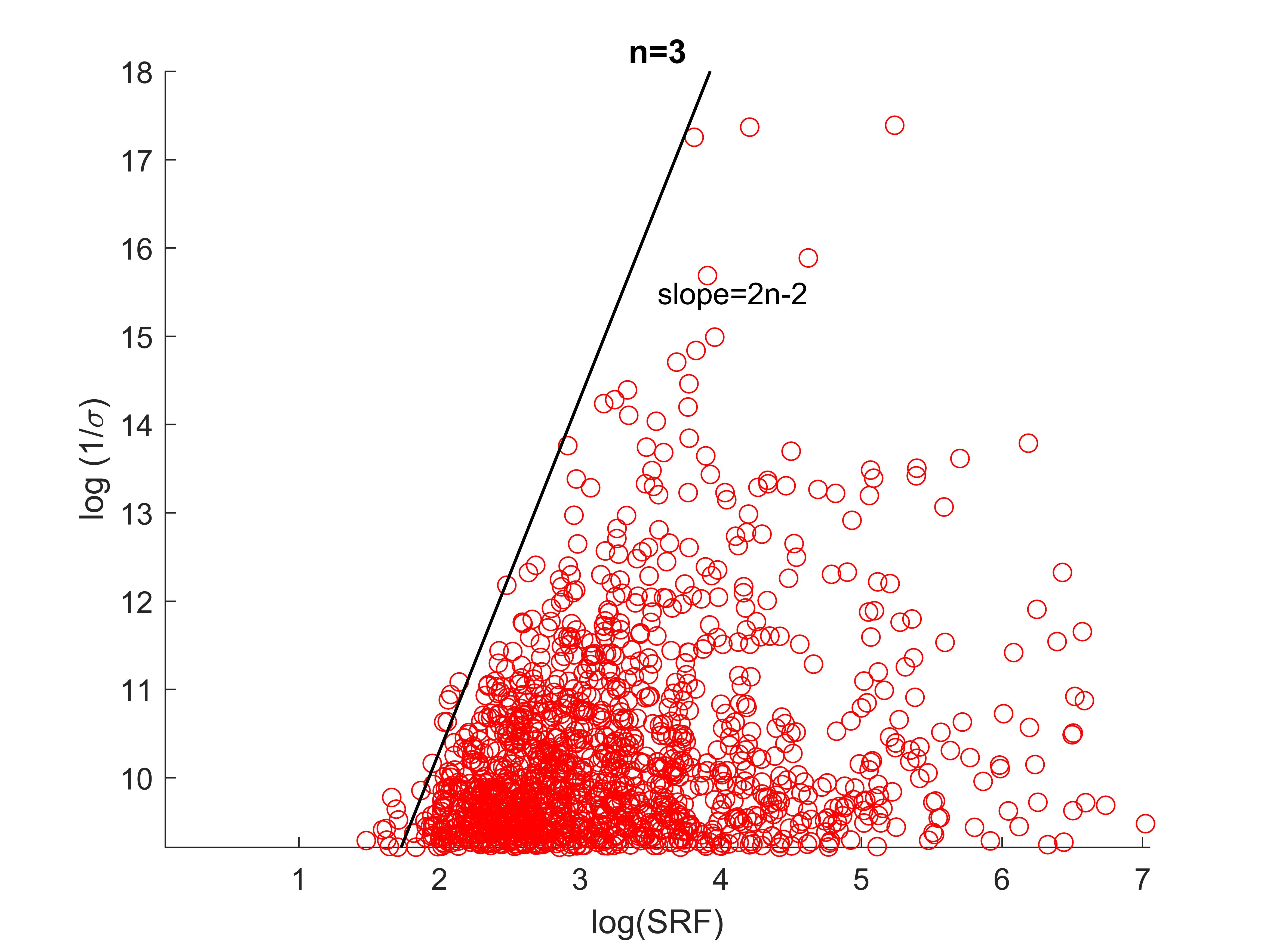
(b) detection fail

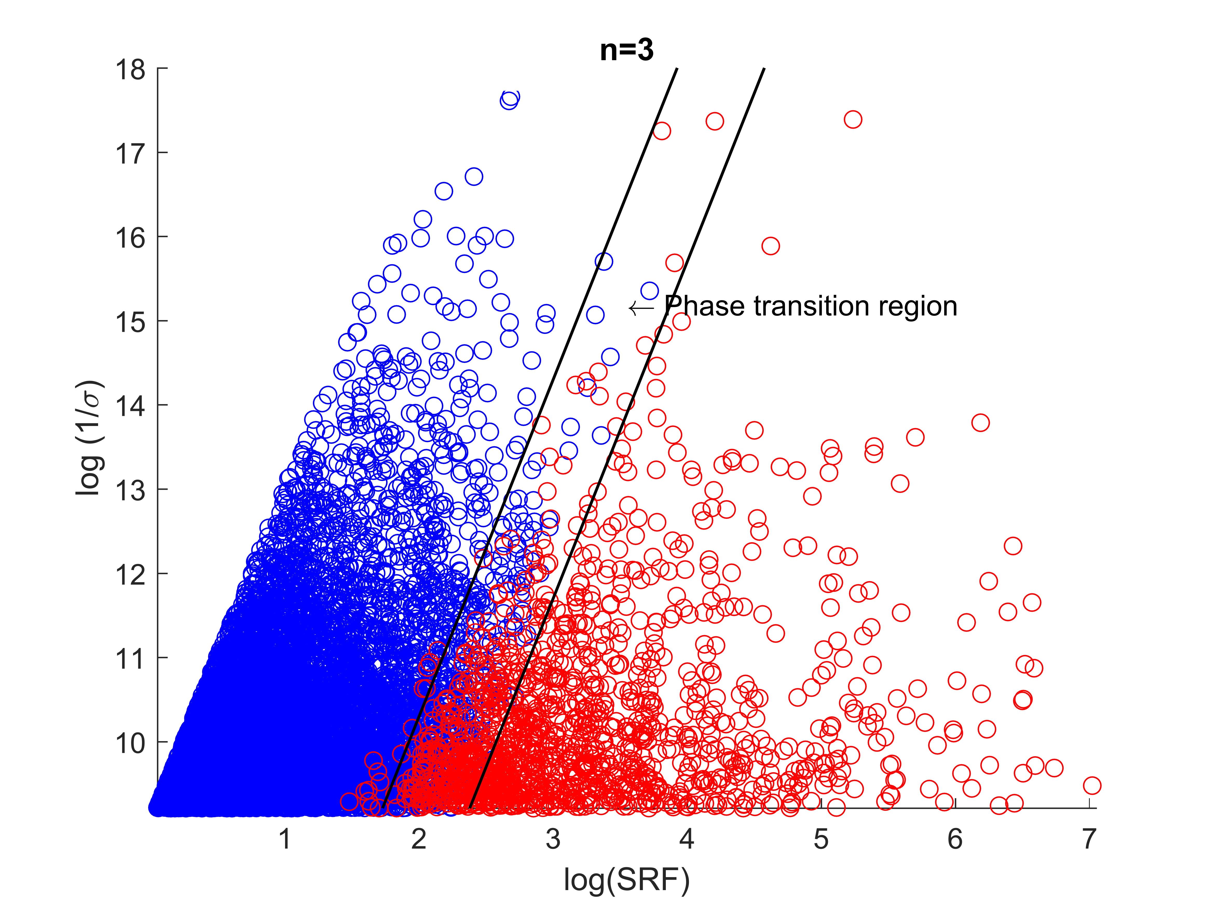
(c) phase transition region

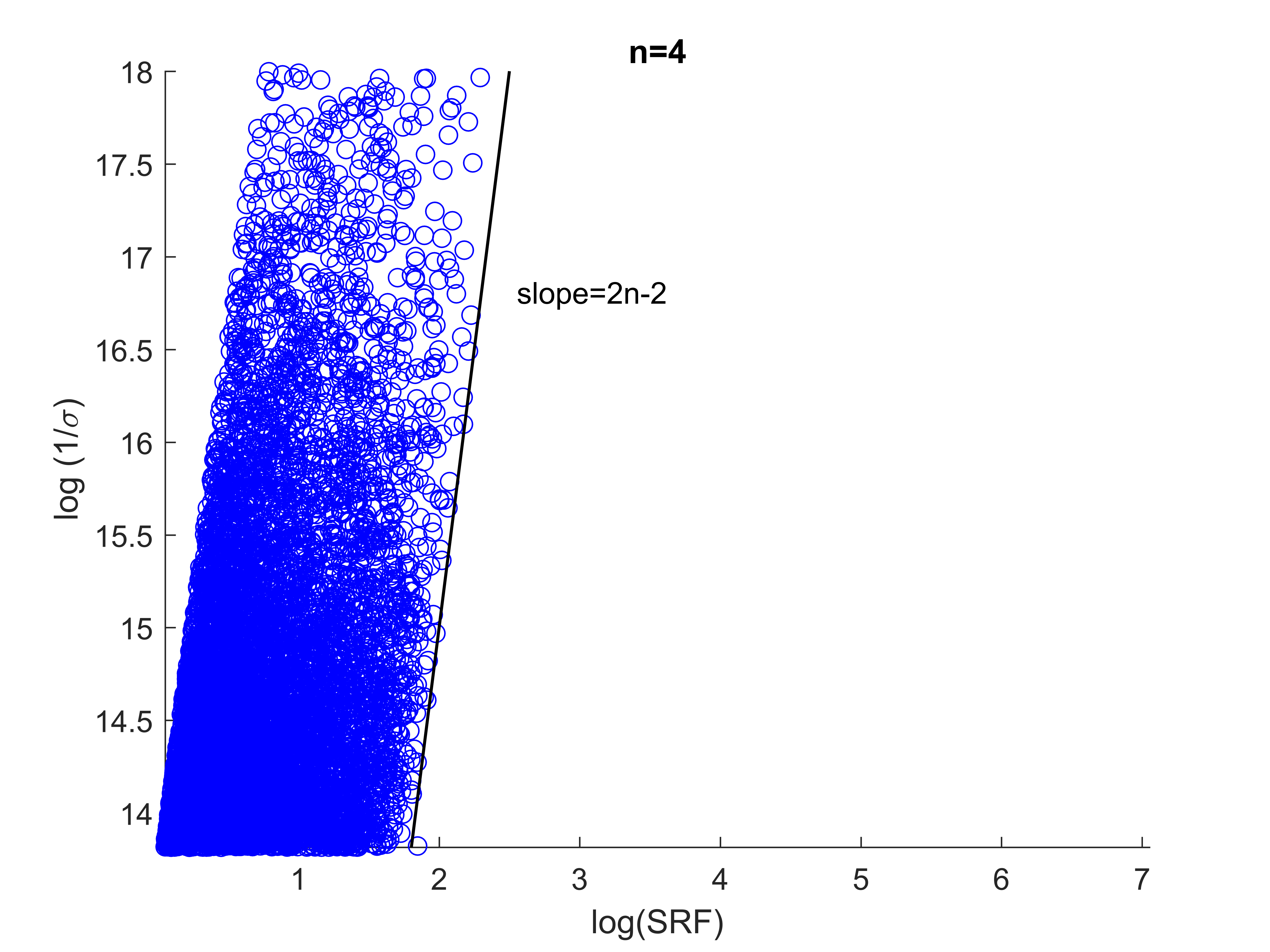
(d) detection success

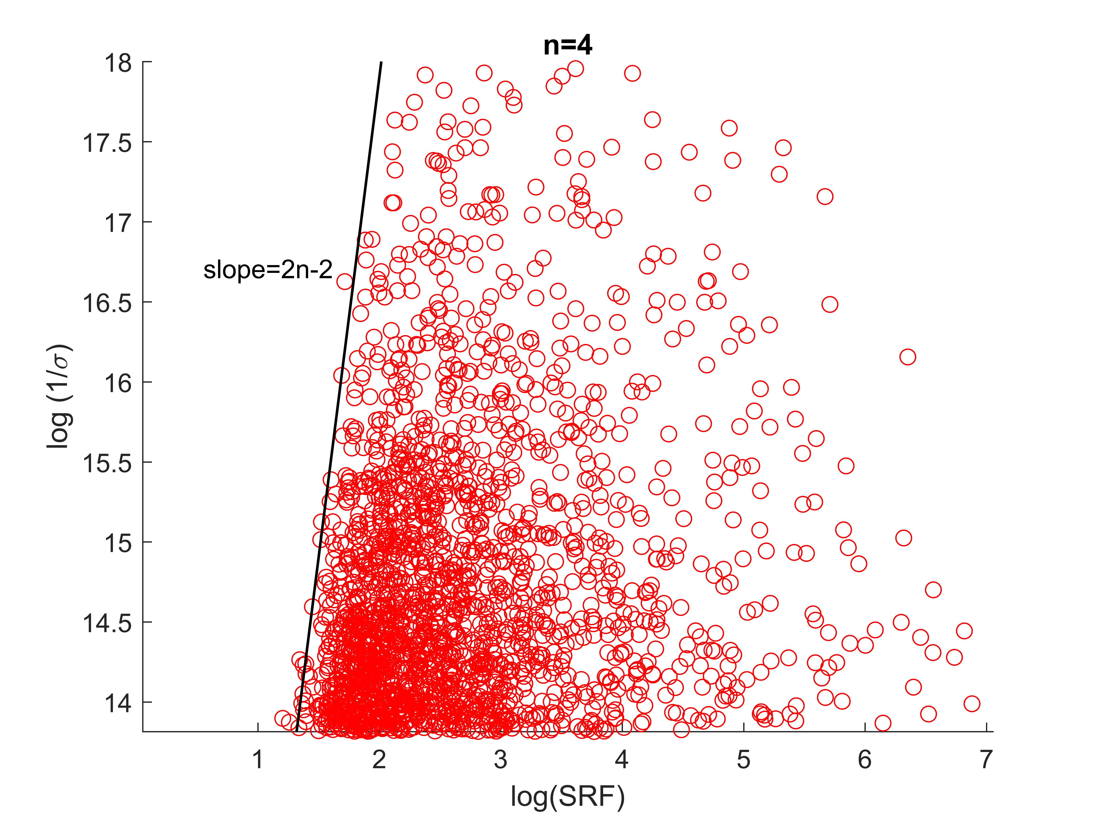
(e) detection fail

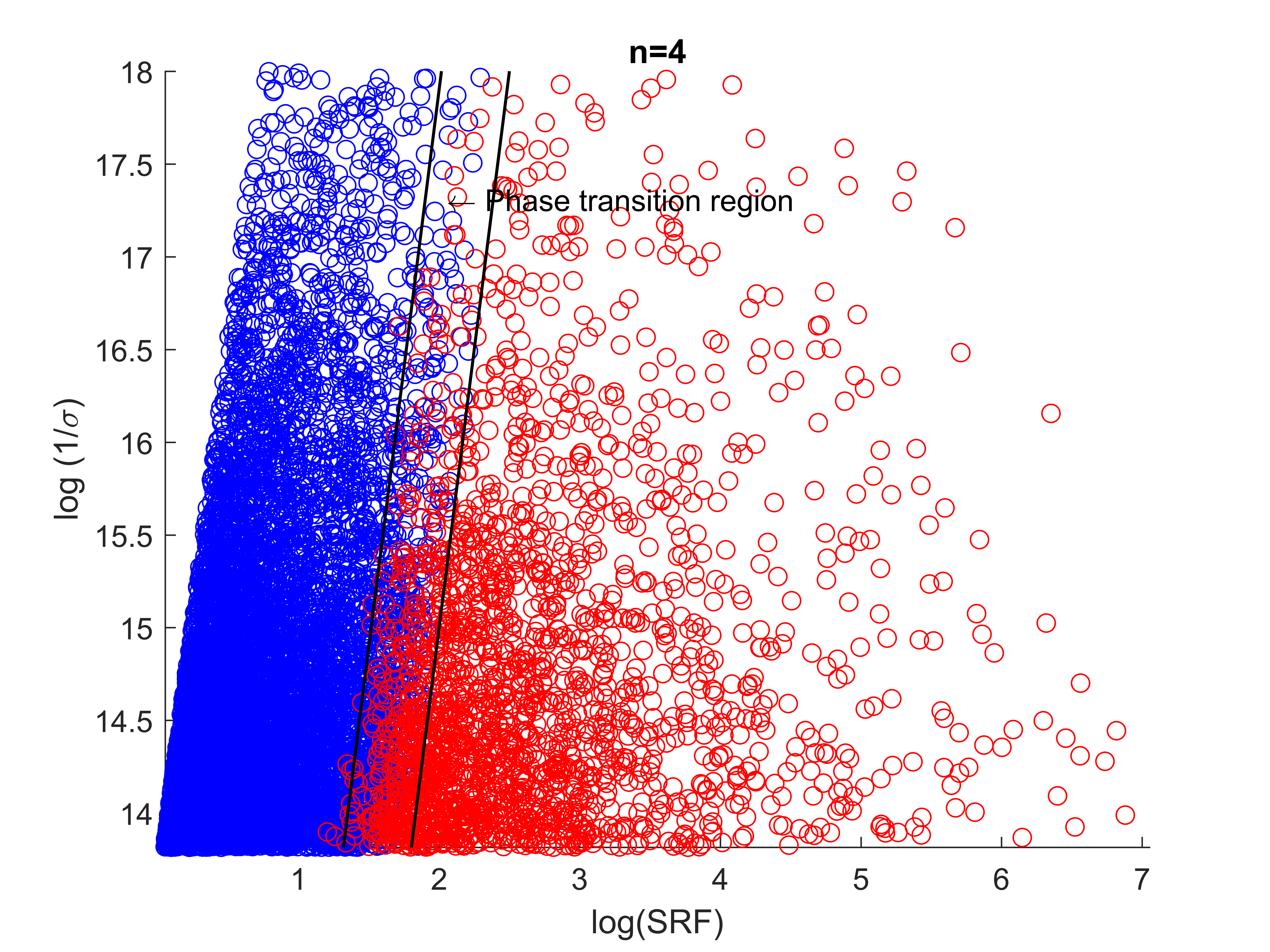
(f) phase transition region

Figure 4.1: Plots of the successful and the unsuccessful number detection by Algorithm 3 depending on the relation between $\log(SRF)$ and $\log(\frac{1}{\sigma})$. (a) illustrates that three point sources can be exactly detected if $\log(\frac{1}{\sigma})$ is above a line of slope $4$ in the parameter space. Conversely, for the same case, (b) shows that the number detection fails if $\log(\frac{1}{\sigma})$ falls below another line of slope $4$. (f) highlights the phase transition region which is bounded by the black slashes in (a) and (b). (d),(e) and (f) illustrate parallel results for four point sources.

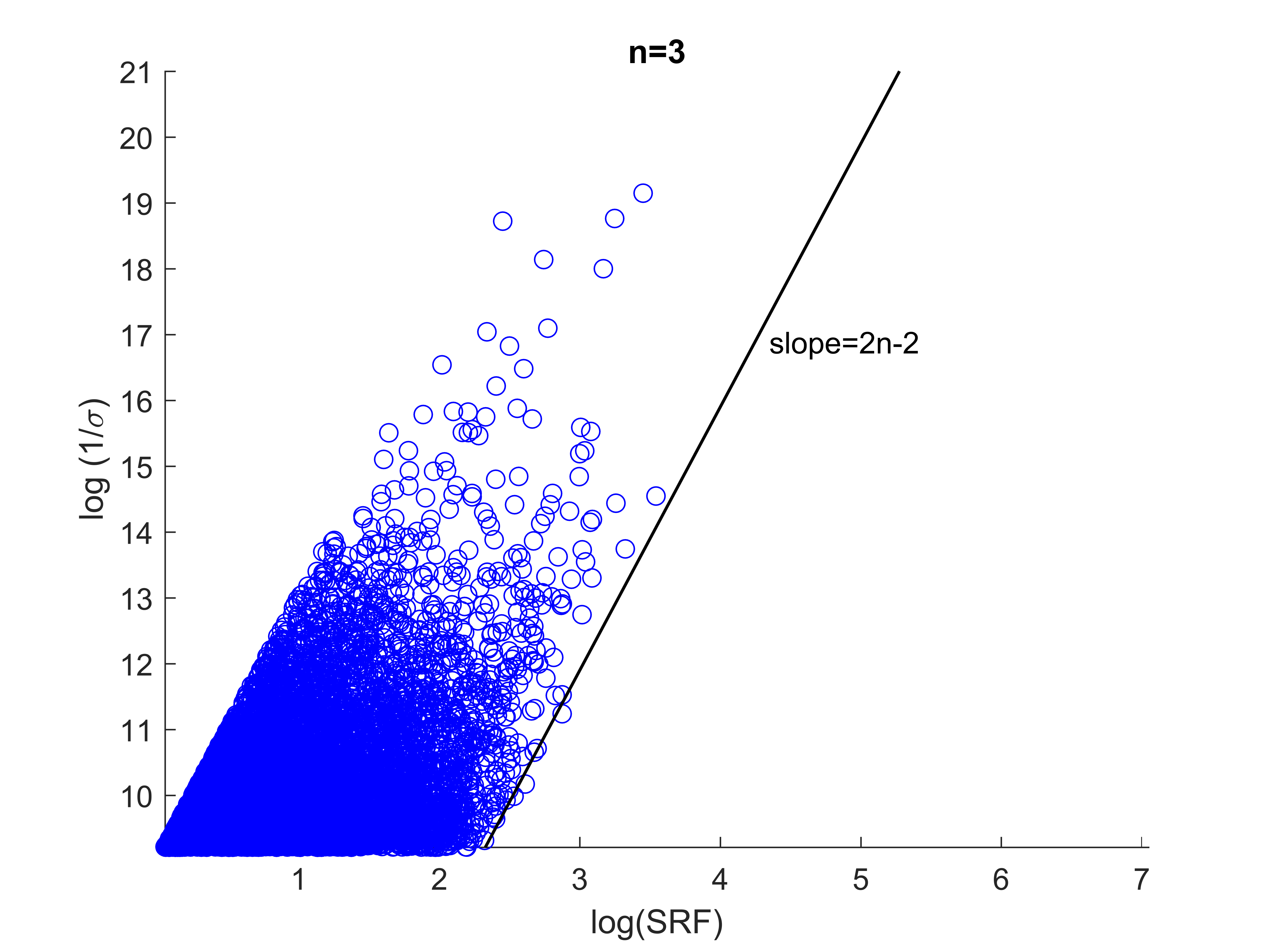
(a) detection success

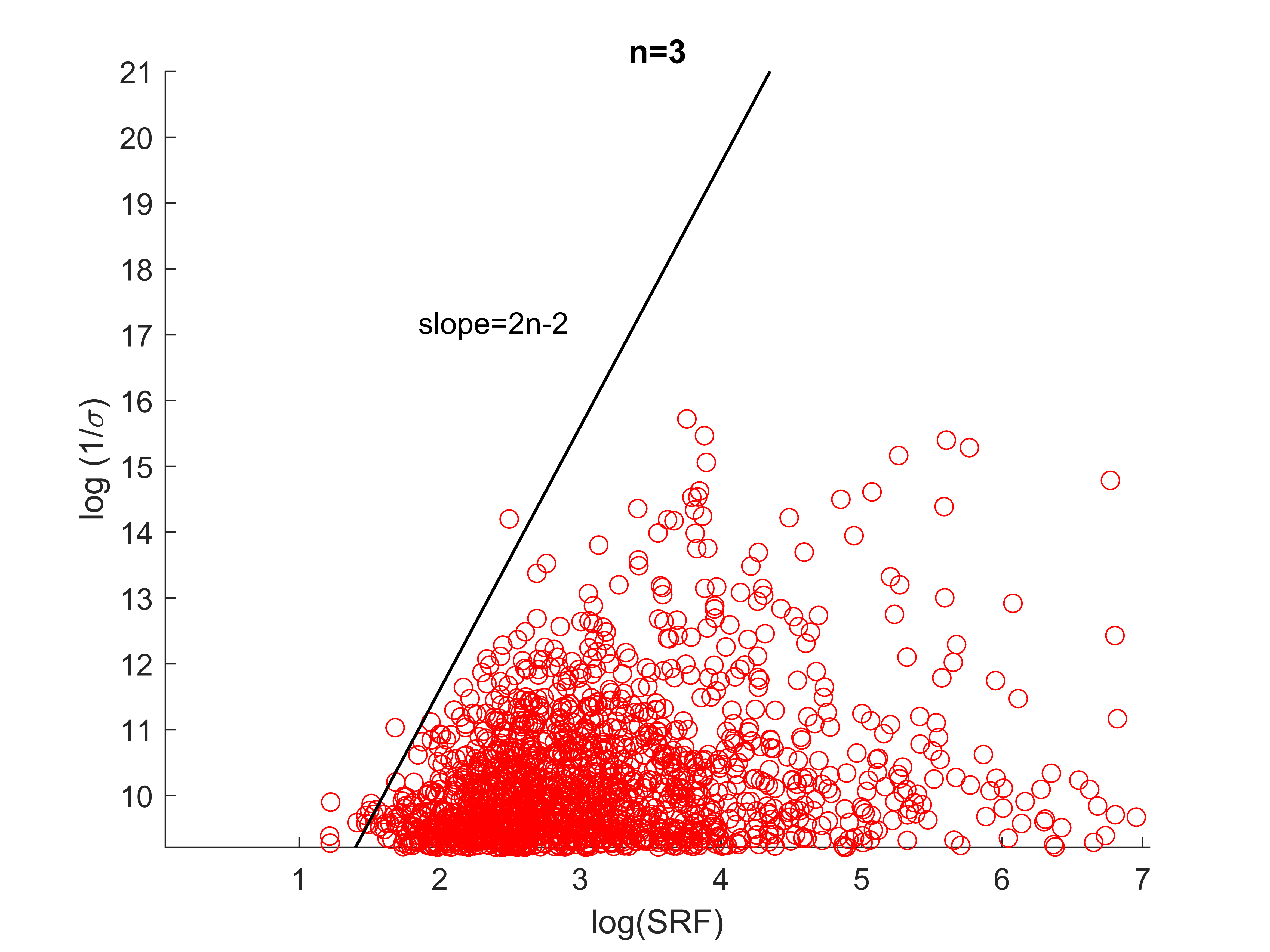
(b) detection fail

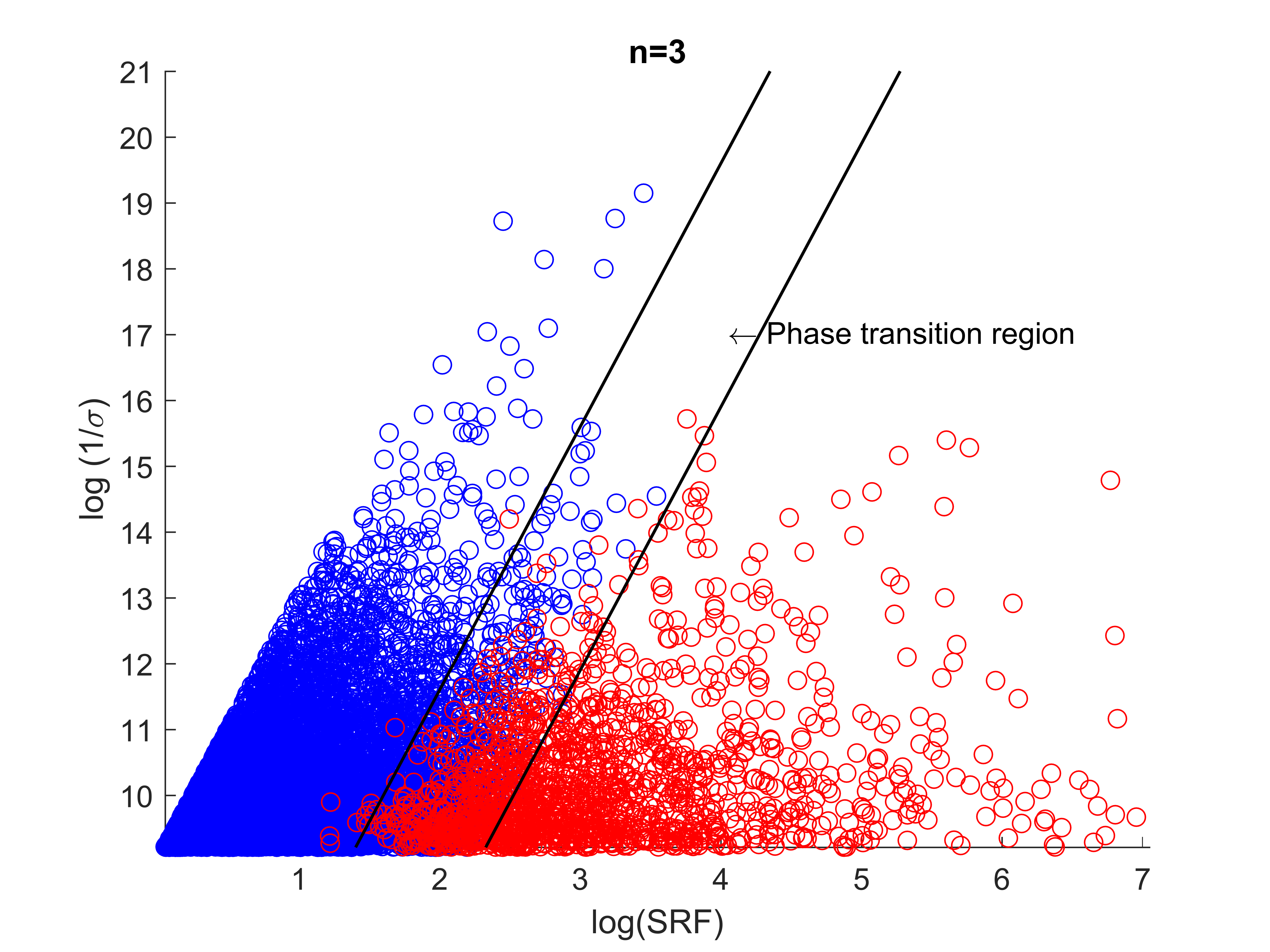
(c) phase transition region

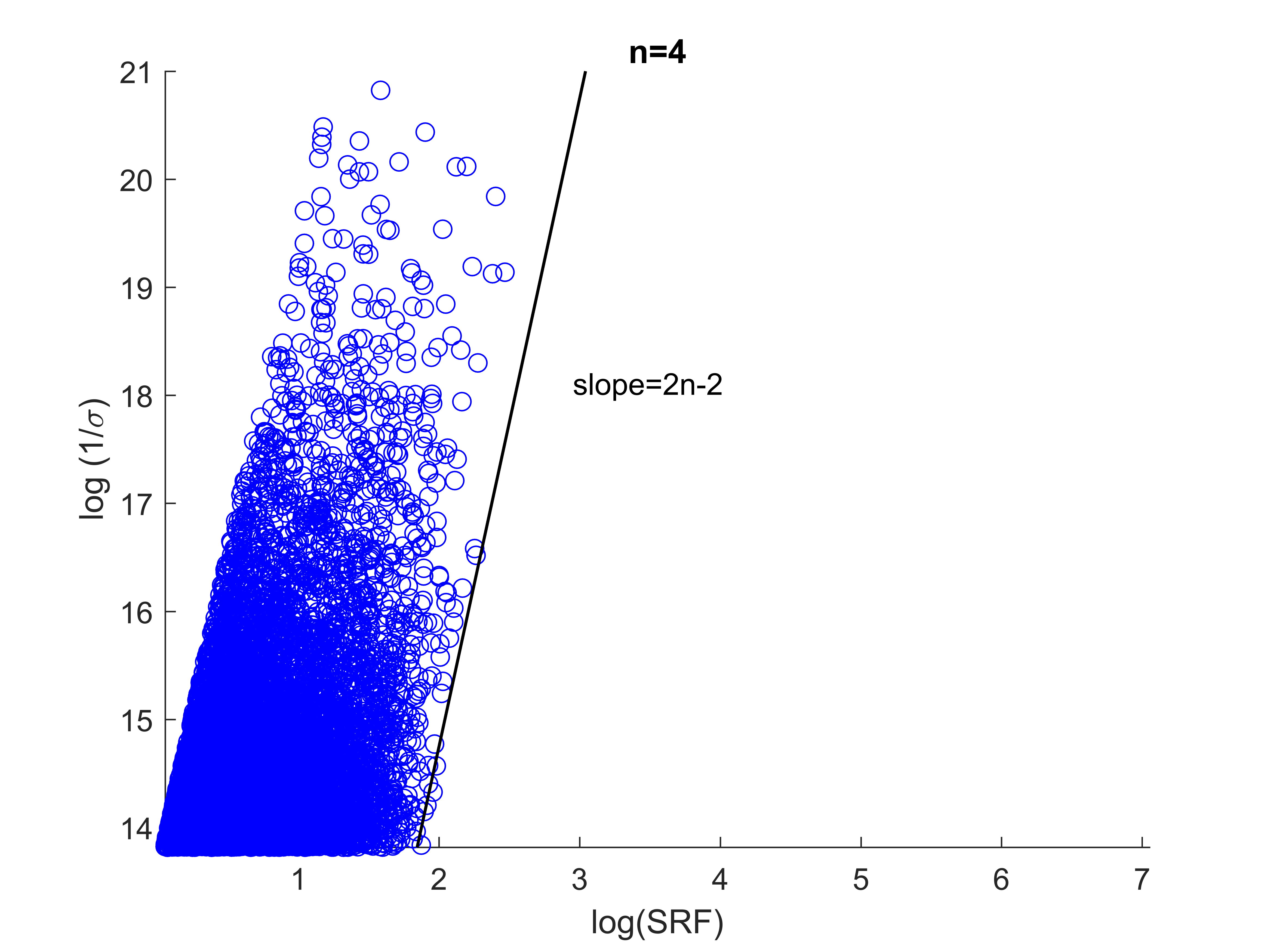
(d) detection success

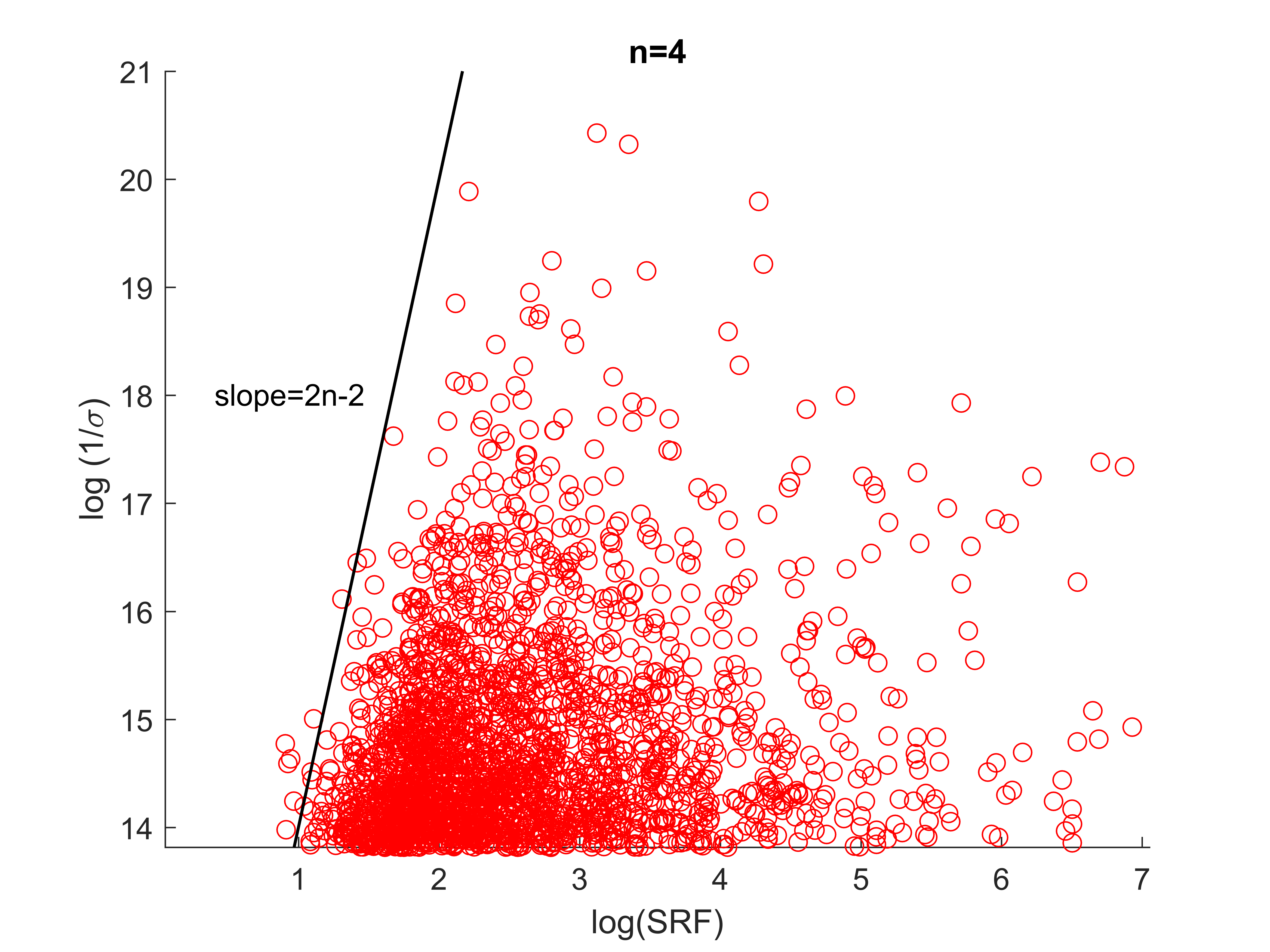
(e) detection fail

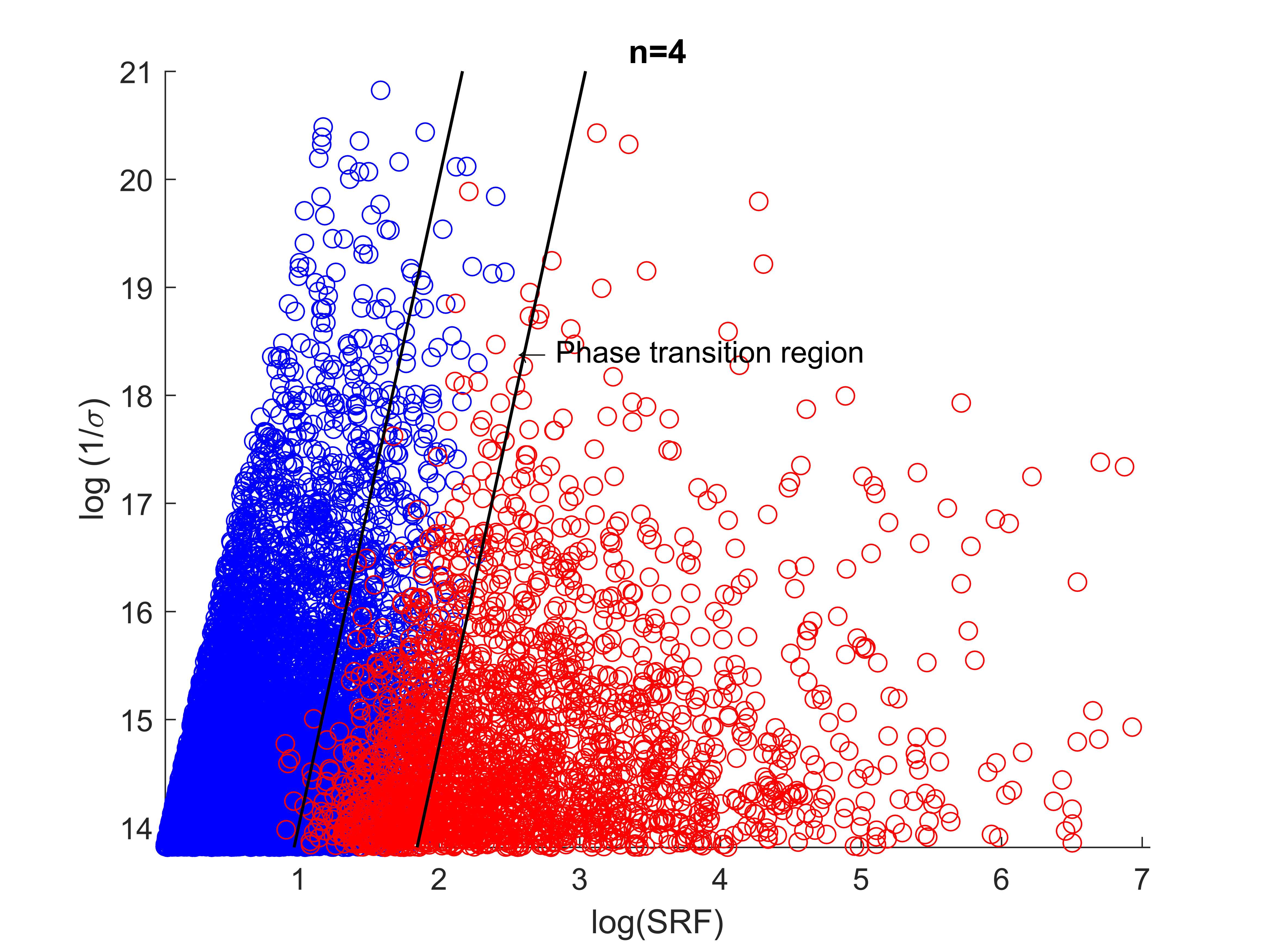
(f) phase transition region

Figure 4.2: Plots of the successful and the unsuccessful number detection by Algorithm 4 depending on the relation between $\log(SRF)$ and $\log(\frac{1}{\sigma})$. (a) illustrates that four point sources can be exactly detected if $\log(\frac{1}{\sigma})$ is above a line of slope $4$ in the parameter space. Conversely, for the same case, (b) shows that the number detection fails if $\log(\frac{1}{\sigma})$ falls below another line of slope $4$. (f) highlights the phase transition region which is bounded by the black slashes in (a) and (b). (d),(e) and (f) illustrate parallel results for four point sources.

5 Subspace projection based support recovery algorithms

In this section, we propose a subspace projection based support recovery algorithm in multi-dimensions. We remark that there are many algorithms that works efficiently to resolve point sources in one dimension. See for instance [47, 52, 58, 50, 28, 29, 18, 44, 43]. Among them, subspace methods such as MUSIC, ESPRIT and Matrix Pencil method are shown to have favourable performance. A typical subspace method estimates the source locations based on the singular value decomposition of the data matrix, see for instance [35, 37]. In [5], the authors provide numerical evidence that the Matrix Pencil method attains the performance bounds of the order of the computational resolution limit. In this paper, we shall use the Matrix Pencil method for the 1-dimensional problem.

5.1 Matrix Pencil Method for support recovery

In this section, we review the Matrix Pencil method for 1-dimensional support recovery problem. Our presentation follows the one in [5].

Let $\bm{\mathbf{H}}_{u}:=\bm{\mathbf{H}}(s)[1:s,:]$ (and $H_{l}:=H(s)[2:s+1,:]$) be the $s\times(s+1)$ matrix obtained from the Hankel matrix $\bm{\mathbf{H}}(s)$ (4.1) by selecting the first $s$ rows (respectively, the $2$ to $s+1$ rows). Then it turns out that, in the noiseless case, $e^{iy_{j}\frac{\Omega}{s}},1\leq j\leq n$, are exactly the nonzero generalized eigenvalues of the pencil $\bm{\mathbf{H}}_{l}-z\bm{\mathbf{H}}_{u}$. In the noisy case, when the sources are well separated, each of the first $n$ nonzero generalized eigenvalues of the pencil $\bm{\mathbf{H}}_{l}-z\bm{\mathbf{H}}_{u}$ is close to $e^{iy_{j}\frac{\Omega}{s}}$ for some $j$ [42]. We summarize the MP method in Algorithm 5 (see also Algorithm 3.1 in [5]), and the interested reader is referred to the widely available literature on the subject (e.g. [29, 28, 42], and references therein) for further details.

Input: Source number $n$, measurement: $\mathbf{Y}(\omega),\bm{\mathbf{\omega}}\in\mathbb{R},||\bm{\mathbf{\omega}}||_{2}\leq\Omega$

1: $r=(M-1)\mod 2s$, $\mathbf{Y}_{new}=(\mathbf{Y}(\omega_{1}),\mathbf{Y}(\omega_{r+1}),\cdots,\mathbf{Y}(\omega_{2sr+1}))^{T}$;

2: Formulate the $(s+1)\times(s+1)$ Hankel matrix $\mathbf{H}(s)$ from $\mathbf{Y}_{new}$, and the matrices $\bm{\mathbf{H}}_{u},\bm{\mathbf{H}}_{l}$;

3: Compute the truncated Singular Value Decomposition (SVD) of $\bm{\mathbf{H}}_{u}$, $\bm{\mathbf{H}}_{l}$ of order $n$:

$$\bm{\mathbf{H}}_{u}=U_{1}\Sigma_{1}V_{1}^{*},\quad\bm{\mathbf{H}}_{l}=U_{2}\Sigma_{2}V_{2}^{*},$$

where $U_{1},U_{2},V_{1},V_{2}$ are $s\times n$ and $\Sigma_{1},\Sigma_{2}$ are $n\times n$;

4: Generate the reduced pencil

$$\mathbf{\hat{H}}_{u}=U_{2}^{*}U_{1}\Sigma_{1}V_{1}^{*}V_{2},\quad\mathbf{\hat{H}}_{l}=\Sigma_{2},$$

where $\mathbf{\hat{H}}_{u}$, $\mathbf{\hat{H}}_{l}$ are $n\times n$;

5: Compute the generalized eigenvalues $\{\hat{z}_{j}\}$ of the reduced pencil $(\mathbf{\hat{H}}_{u},\mathbf{\hat{H}}_{l})$, and put $\{\hat{y}_{j}\}=\{\angle\hat{z}_{j}\},j=1,\cdots,n$;

Return $\{\hat{y}_{j}\}$

Algorithm 5 The Matrix Pencil algorithm

5.2 Subspace projection based Matrix Pencil Method for support recovery

In this section we propose a subspace projection based Matrix Pencil algorithm for the support recovery in multi-dimensions. We refer the readers to ([13, 59, 32, 72, 71, 65, 69, 23, 68, 70]) for other algorithms in various settings in dimension two or three.

As is indicated by the proof of Theorem 2.7, when sources are well separated in $\mathbb{R}^{k+1}$, there exist two unit vectors $\bm{\mathbf{v}}_{1},\bm{\mathbf{v}}_{2}$ so that the projection of source locations in the two $k$-dimensional subspaces $\bm{\mathbf{v}}_{1}^{\perp}$ and $\bm{\mathbf{v}}_{2}^{\perp}$ can be stably recovered simultaneously. We can then find the original source positions from their projections. To demonstrate the idea, We first consider the 2-dimensional case. Let $N=\frac{(n+2)(n-1)}{2}$ and

$$\bm{\mathbf{v}}_{q}=(\cos\phi_{1,q},\ \sin{\phi_{1,q}})^{T},\quad\phi_{1,q}=\frac{q\pi}{N},1\leq q\leq N.$$ (5.1)

For each 1-dimensional subspace $\bm{\mathbf{v}}_{q}^{\perp}$, we first recover the source number therein and choose only those where the recovered number is exactly $n$. We then recover the projection of the source positions in each of those 1-dimensional subspace using the 1-dimensional Matrix Pencil method. We choose two vectors, denoted by $\bm{\mathbf{v}}_{1},\bm{\mathbf{v}}_{2}$, from those $\bm{\mathbf{v}}_{q}$’s so that the recovered positions in $\bm{\mathbf{v}}_{1}^{\perp},\bm{\mathbf{v}}_{2}^{\perp}$ have respectively the largest and second largest minimum separation distance. We remark that, when $N$ is large, one can require additionally that $\bm{\mathbf{v}}_{1}$ is not too much correlated to $\bm{\mathbf{v}}_{2}$, say $|\bm{\mathbf{v}}_{1}\cdot\bm{\mathbf{v}}_{2}|\leq c$ for some constant $0<c<1$ to ensure that the reconstruction of 2-dimensional locations from their projections on $\bm{\mathbf{v}}_{1}^{\perp},\bm{\mathbf{v}}_{2}^{\perp}$ is stable.

We next construct the original source locations from their projection on the 1-dimensional subspaces $\bm{\mathbf{v}}_{1}^{\perp}$ and $\bm{\mathbf{v}}_{2}^{\perp}$. This is usually called the pair matching in DOA problem that ad hoc schemes [73, 31, 10, 71] are derived to associate the estimated azimuth and elevation angles. In our paper, this can be done in the following manner. From the projected locations on the subspaces $\bm{\mathbf{v}}_{1}^{\perp},\bm{\mathbf{v}}_{2}^{\perp}$, we first form a grid of $n^{2}$ points $\bm{\mathbf{z}}_{1,1},\bm{\mathbf{z}}_{1,2},\cdots,\bm{\mathbf{z}}_{n,n}$. It can be shown that the original source positions are close to these grid points. These grid points reduce the off-the-grid recovery problem to an on-the-grid one. We then employ an enumeration method to recover the source locations from these grid points. To be more specific, we define $G(\bm{\mathbf{z}}_{1,j_{1}},\cdots,\bm{\mathbf{z}}_{n,j_{n}})=\big{(}e^{i\bm{\mathbf{z}}_{1,j_{1}}\bm{\mathbf{\omega}}}\ e^{i\bm{\mathbf{z}}_{2,j_{2}}\bm{\mathbf{\omega}}}\ \cdots\ e^{i\bm{\mathbf{z}}_{n,j_{n}}\bm{\mathbf{\omega}}}\big{)}$ and solve the following optimization problem by enumeration,

$$\min_{\mathbf{\hat{a}},\pi\in\zeta(n)}||G(\bm{\mathbf{z}}_{1,\pi_{1}},\cdots,\bm{\mathbf{z}}_{n,\pi_{n}})\mathbf{\hat{a}}-\bm{\mathbf{Y}}||_{2},$$ (5.2)

where $\zeta(n)$ is the set of all permutations of $\{1,\cdots,n\}$. We note that the computational complexity of the enumeration is low when $n$ is not large. We summarize the algorithm in Algorithm 6 below.

Input: Noise level $\sigma$, source number $n$,and measurement: $\mathbf{Y}(\bm{\mathbf{\omega}}),\bm{\mathbf{\omega}}\in\mathbb{R}^{2},||\bm{\mathbf{\omega}}||_{2}\leq\Omega$

Input: A large enough $N$, and corresponding $N$ unit vectors $\bm{\mathbf{v}}(\phi),\phi\in\Big{\{}\frac{\pi}{N},\frac{2\pi}{N},\cdots,\pi\Big{\}}$

1:for $\phi\in\Big{\{}\frac{\pi}{N},\frac{2\pi}{N},\cdots,\pi\Big{\}}$ do

       Input $\sigma$ and $\mathbf{Y}(\bm{\mathbf{\omega}}),\bm{\mathbf{\omega}}\in\bm{\mathbf{v}}(\phi_{1})^{\perp}$ to Algorithm 2 to recover the projected source number $\hat{n}$;

       if $\hat{n}==n$ then

             Input $\sigma,\mathbf{Y}(\bm{\mathbf{\omega}}),\bm{\mathbf{\omega}}\in\bm{\mathbf{v}}(\phi_{1})^{\perp}$ and $\hat{n}$ to Algorithm 5, save the output of Algorithm 5 as $\bm{\mathbf{\hat{p}}}_{1},\cdots,\mathbf{\hat{p}}_{n}$;

      

2: Choose two vectors, denoted by $\bm{\mathbf{v}}_{1},\bm{\mathbf{v}}_{2}$, from those $\bm{\mathbf{v}}(\phi)$’s so that the recovered positions $\bm{\mathbf{\hat{y}}}_{j}(\bm{\mathbf{v}}_{1}^{\perp})$’s, $\mathbf{\hat{y}}_{j}(\bm{\mathbf{v}}_{2}^{\perp})$’s in spaces $\bm{\mathbf{v}}_{1}^{\perp},\bm{\mathbf{v}}_{2}^{\perp}$ have respectively the largest and second largest minimum separation distance;

3:Construct the $n^{2}$ grid points $\bm{\mathbf{z}}_{1,1},\bm{\mathbf{z}}_{1,2},\cdots,\bm{\mathbf{z}}_{n,n}$ by considering the intersection points of lines $\mathbf{\hat{y}}_{q}(\bm{\mathbf{v}}_{j}^{\perp})+\lambda\bm{\mathbf{v}}_{j},\ \lambda\in\mathbb{R},\ q=1,\cdots,n,\ j=1,2$;

4: Solve the following optimization problem by enumeration,

$$\min_{\mathbf{\hat{a}},\pi\in\zeta(n)}||G(\bm{\mathbf{z}}_{1,\pi_{1}},\cdots,\bm{\mathbf{z}}_{n,\pi_{n}})\mathbf{\hat{a}}-\bm{\mathbf{Y}}||_{2}$$

where $\zeta(n)$ is the set of all permutations of $\{1,\cdots,n\}$ and $G(\bm{\mathbf{z}}_{1,\pi_{1}},\cdots,\bm{\mathbf{z}}_{n,\pi_{n}})=\big{(}e^{i\bm{\mathbf{z}}_{1,\pi_{1}}\bm{\mathbf{\omega}}}\ e^{i\bm{\mathbf{z}}_{2,\pi_{2}}\bm{\mathbf{\omega}}}\ \cdots\ e^{i\bm{\mathbf{z}}_{n,\pi_{n}}\bm{\mathbf{\omega}}}\big{)}$;

6: The minimizer $\bm{\mathbf{z}}_{1,\pi_{1}},\cdots,\bm{\mathbf{z}}_{n,\pi_{n}}$’s are the recovered source locations $\mathbf{\hat{y}}_{1},\cdots,\mathbf{\hat{y}}_{n}$;

Return $\mathbf{\hat{y}}_{1},\cdots,\mathbf{\hat{y}}_{n}$.

Algorithm 6 Two-dimensional subspace projection based support recovery algorithm

Now we present the algorithm for 3-dimensional support recovery. For point sources located in dimension three, we first recover their projections in two properly chosen 2-dimensional subspaces. Precisely, we choose the unit vectors

$$\bm{\mathbf{v}}(\phi_{1},\phi_{2})=(\cos\phi_{1},\ \sin{\phi_{1}}\cos{\phi_{2}},\ \sin\phi_{1}\sin\phi_{2})^{T},\quad\phi_{1},\phi_{2}\in\Big{\{}\frac{\pi}{2N},\frac{2\pi}{2N},\cdots,\frac{\pi}{2}\Big{\}},$$ (5.3)

where $N=\lfloor(\frac{n(n-1)}{2})^{\frac{1}{2}}\rfloor+1$. Utilizing measurement in each of the 2-dimensional subspaces $\bm{\mathbf{v}}(\phi_{1},\phi_{2})^{\perp}$, we can recover the source locations in some of these spaces stably by Algorithm 6. We choose the two subspaces where the minimum separation distance of the reconstructed project source locations is the largest and second largest and denote them by $\bm{\mathbf{v}}_{1}^{\perp}$ and $\bm{\mathbf{v}}_{2}^{\perp}$ respectively. The recovered locations in these two subspaces are denoted by $\mathbf{\hat{y}}_{j}(\bm{\mathbf{v}}_{1}^{\perp})$, $1\leq j\leq n$, and $\mathbf{\hat{y}}_{j}(\bm{\mathbf{v}}_{2}^{\perp})$, $1\leq j\leq n$, respectively. For each pair of $j,p$, we construct two lines $\bm{\mathbf{\hat{y}}}_{j}(\bm{\mathbf{v}}_{1}^{\perp})+\lambda\bm{\mathbf{v}}_{1}$ and $\bm{\mathbf{\hat{y}}}_{p}(\bm{\mathbf{v}}_{2}^{\perp})+\lambda\bm{\mathbf{v}}_{2}$ and denote them by $l_{1,j},l_{2,p}$ respectively. For the line pair $(l_{1,j},l_{2,p})$, we find the two points $\bm{\mathbf{c}}_{1,j}\in l_{1,j},\bm{\mathbf{c}}_{2,p}\in l_{2,j}$ which minimize the distance of the two lines. We then choose the middle point $\frac{\bm{\mathbf{c}}_{1,j}+\bm{\mathbf{c}}_{2,p}}{2}$ as a possible source location if $\|\bm{\mathbf{c}}_{1,j}-\bm{\mathbf{c}}_{2,p}\|_{2}$ is not great than the two minimum separation distances in $\bm{\mathbf{v}}_{1}^{\perp}$ and $\bm{\mathbf{v}}_{2}^{\perp}$. Finally by solving an optimization problem with these possible source locations, we can reconstruct stably the original source positions. The procedure is similar to the two dimensional case and is summarized in Algorithm 7 below.

Input: Noise level $\sigma$, source number $n$,and measurement: $\mathbf{Y}(\bm{\mathbf{\omega}}),\bm{\mathbf{\omega}}\in\mathbb{R}^{2},||\bm{\mathbf{\omega}}||_{2}\leq\Omega$

Input: A large enough $N$, and corresponding $N^{2}$ unit vectors $\bm{\mathbf{v}}(\phi_{1},\phi_{2}),\phi_{1},\phi_{2}\in\Big{\{}\frac{\pi}{2N},\frac{2\pi}{2N},\cdots,\frac{\pi}{2}\Big{\}}$

1:for $\phi_{1},\phi_{2}\in\Big{\{}\frac{\pi}{2N},\frac{2\pi}{2N},\cdots,\frac{\pi}{2}\Big{\}}$ do

       Input $\sigma$ and $\mathbf{Y}(\bm{\mathbf{\omega}}),\bm{\mathbf{\omega}}\in\bm{\mathbf{v}}(\phi_{1},\phi_{2})^{\perp}$ to Algorithm 3 to recover the projected source number $\hat{n}$;

       if $\hat{n}==n$ then

             Input $\sigma,\mathbf{Y}(\bm{\mathbf{\omega}}),\bm{\mathbf{\omega}}\in\bm{\mathbf{v}}(\phi_{1},\phi_{2})^{\perp}$ and $\hat{n}$ to Algorithm 6, save the output as $\bm{\mathbf{\hat{p}}}_{1},\cdots,\mathbf{\hat{p}}_{n}$;

      

2:Choose two vectors, denoted by $\bm{\mathbf{v}}_{1},\bm{\mathbf{v}}_{2}$, from those $\bm{\mathbf{v}}(\phi_{1},\phi_{2})$’s so that the recovered projected positions $\bm{\mathbf{\hat{y}}}_{j}(\bm{\mathbf{v}}_{1}^{\perp})^{\prime}s,\mathbf{\hat{y}}_{j}(\bm{\mathbf{v}}_{2}^{\perp})^{\prime}s$ in spaces $\bm{\mathbf{v}}_{1}^{\perp},\bm{\mathbf{v}}_{2}^{\perp}$ have respectively the largest and the second largest minimum separation distance (denoted by $d_{\min},\hat{d}_{\min}$ respectively);

3: Denote the line $\bm{\mathbf{\hat{y}}}_{j}(\bm{\mathbf{v}}_{1}^{\perp})+\lambda\bm{\mathbf{v}}_{1}$ by $l_{1,j}$ and the line $\bm{\mathbf{\hat{y}}}_{p}(\bm{\mathbf{v}}_{2}^{\perp})+\lambda\bm{\mathbf{v}}_{2}$ by $l_{2,p}$. For every pair of lines $l_{1,j},l_{2,p}$, find the two nearest points in the two lines and denote them by $\bm{\mathbf{c}}_{1,j},\bm{\mathbf{c}}_{2,p}$. If $||\bm{\mathbf{c}}_{1,j}-\bm{\mathbf{c}}_{2,p}||<\min(d_{\min},\hat{d}_{\min})$, consider the point $\frac{\bm{\mathbf{c}}_{1,j}+\bm{\mathbf{c}}_{2,p}}{2}$ as a candidate location and denote it by $\bm{\mathbf{z}}_{j,p}$. Ignore those $\frac{\bm{\mathbf{c}}_{1,j}+\bm{\mathbf{c}}_{2,p}}{2}$ if $||\bm{\mathbf{c}}_{1,j}-\bm{\mathbf{c}}_{2,p}||\geq\min(d_{\min},\hat{d}_{\min})$;

4: Solve the following optimization problem over the above $\bm{\mathbf{z}}_{j,p}$’s,

$$\min_{\mathbf{\hat{a}},j_{p}\neq j_{q},p\neq q}||G(\bm{\mathbf{z}}_{1,j_{1}},\cdots,\bm{\mathbf{z}}_{n,j_{n}})\mathbf{\hat{a}}-\bm{\mathbf{Y}}||_{2}$$

where $G(\bm{\mathbf{z}}_{1,j_{1}},\cdots,\bm{\mathbf{z}}_{n,j_{n}})=\big{(}e^{i\bm{\mathbf{z}}_{1,j_{1}}\bm{\mathbf{\omega}}}\ e^{i\bm{\mathbf{z}}_{2,j_{2}}\bm{\mathbf{\omega}}}\ \cdots\ e^{i\bm{\mathbf{z}}_{n,j_{n}}\bm{\mathbf{\omega}}}\big{)}$;

5: The minimizer $\bm{\mathbf{z}}_{1,j_{1}},\cdots,\bm{\mathbf{z}}_{n,j_{n}}$’s are the recovered source locations $\mathbf{\hat{y}}_{1},\cdots,\mathbf{\hat{y}}_{n}$;

Return $\mathbf{\hat{y}}_{1},\cdots,\mathbf{\hat{y}}_{n}$.

Algorithm 7 Three-dimensional subspace projection based support recovery algorithm

5.3 Numerical experiments and phase transition

We perform numerical experiments to demonstrate the phase transition phenomenon regarding to the super-resolution factor and the SNR for the support recovery in dimension two and three. In view of the computational resolution limit for support recovery (which is of the order $O(\frac{1}{\Omega}\big{(}\frac{\sigma}{m_{\min}}\big{)}^{\frac{1}{2n-1}})$), recovering $5$ closely-spaced point sources demands extremely low noise level. Therefore, in the experiments we only consider the case of three and four sources. For the $2$-dimensional case, we fix $\Omega=1$ and consider $n$ ($n=3$ or $4$) point sources separated with minimum separation $d_{\min}$. We perform 10000 random experiments (the randomness is in the choice of $(d_{\min},\sigma,\bm{\mathbf{y}}_{j},a_{j})$ to recover the source locations using Algorithm 8. For the $3$-dimensional case, we conduct $10000$ random experiments under the same setup. As is shown in Figure 5.1 and 5.2, in each case, two lines with slope $2n-1$ strictly separate the blue points (successful cases) and red points (unsuccessful cases), and in-between is the phase transition region. This is exactly the predicted phase transition phenomenon by our theory of computational resolution limit for support recovery. It also demonstrates that the proposed support recovery algorithm can resolve the location of point sources in the regime where the separation distance is on the order of the computational resolution limit.

Input: Sources $\mu=\sum_{j=1}^{n}a_{j}\delta_{\bm{\mathbf{y}}_{j}}$, Noise level $\sigma$

Input: Measurements: $\mathbf{Y}(\bm{\mathbf{\omega}}),||\bm{\mathbf{\omega}}||_{2}\leq\Omega$

1: $\text{Successnumber}=0$;

2: Input source number $n$ and measurement $\bm{\mathbf{Y}}$ to Algorithm 6 (Algorithm 7 for $3$-dimensional case) and save the output as $\bm{\mathbf{y}}_{1},\cdots,\bm{\mathbf{y}}_{n}$;

for each $1\leq j\leq n$ do

       Compute the error for the source location $\bm{\mathbf{y}}_{j}$: $e_{j}:=\min_{\mathbf{\hat{y}}_{l},l=1,\cdots,n}||\mathbf{\hat{y}}_{l}-\bm{\mathbf{y}}_{j}||_{2}$;

       The source location $\bm{\mathbf{y}}_{j}$ is recovered successfully if

$$e_{j}<\frac{\min_{p\neq j}||\bm{\mathbf{y}}_{p}-\bm{\mathbf{y}}_{j}||_{2}}{3};$$

and

$$\text{Successnumber}=\text{Successnumber}+1;$$

if $\text{Successnumber}==n$ then

       Return Success

else

      Return Fail

Algorithm 8 A single experiment

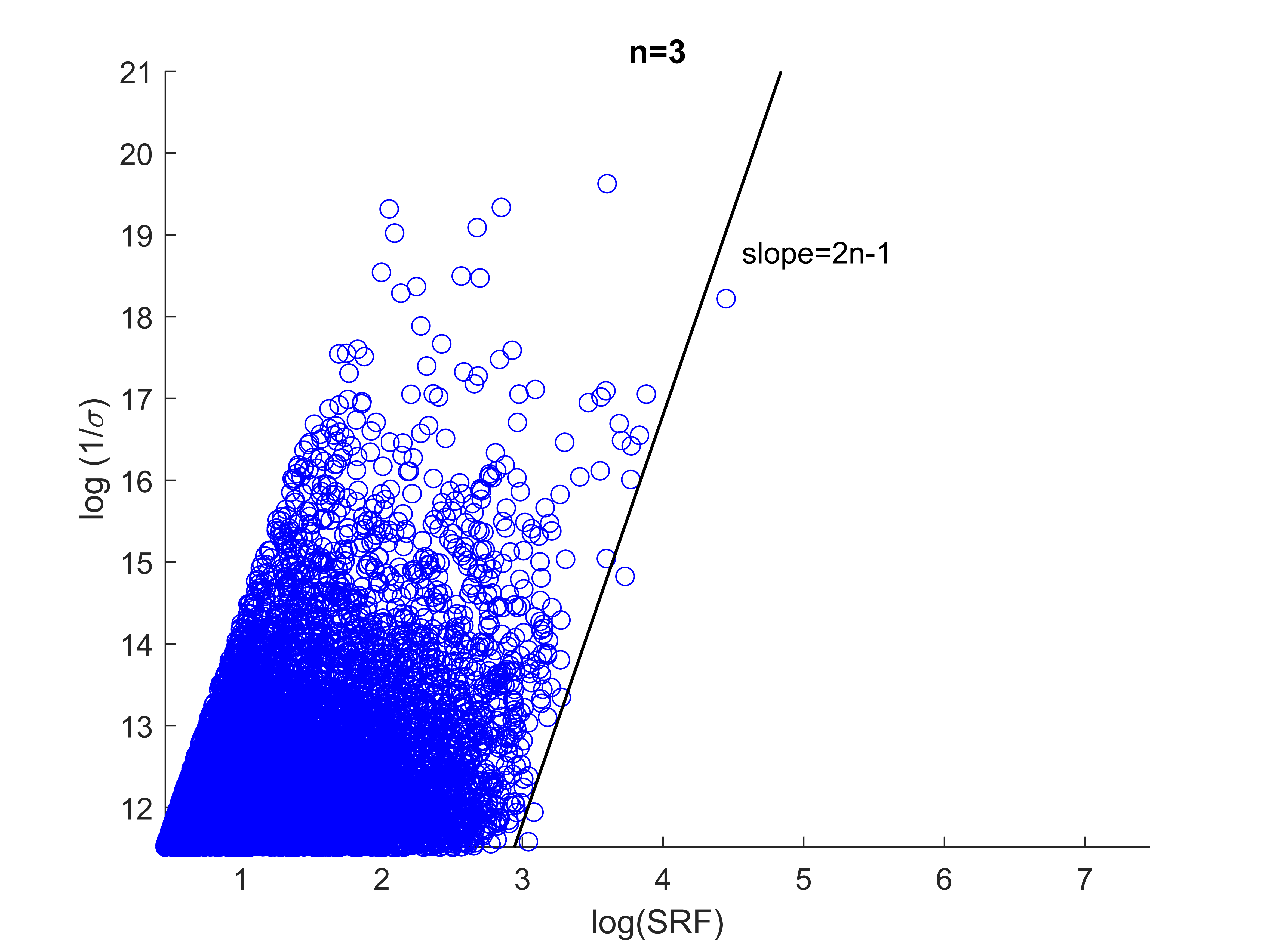
(a) recovery success

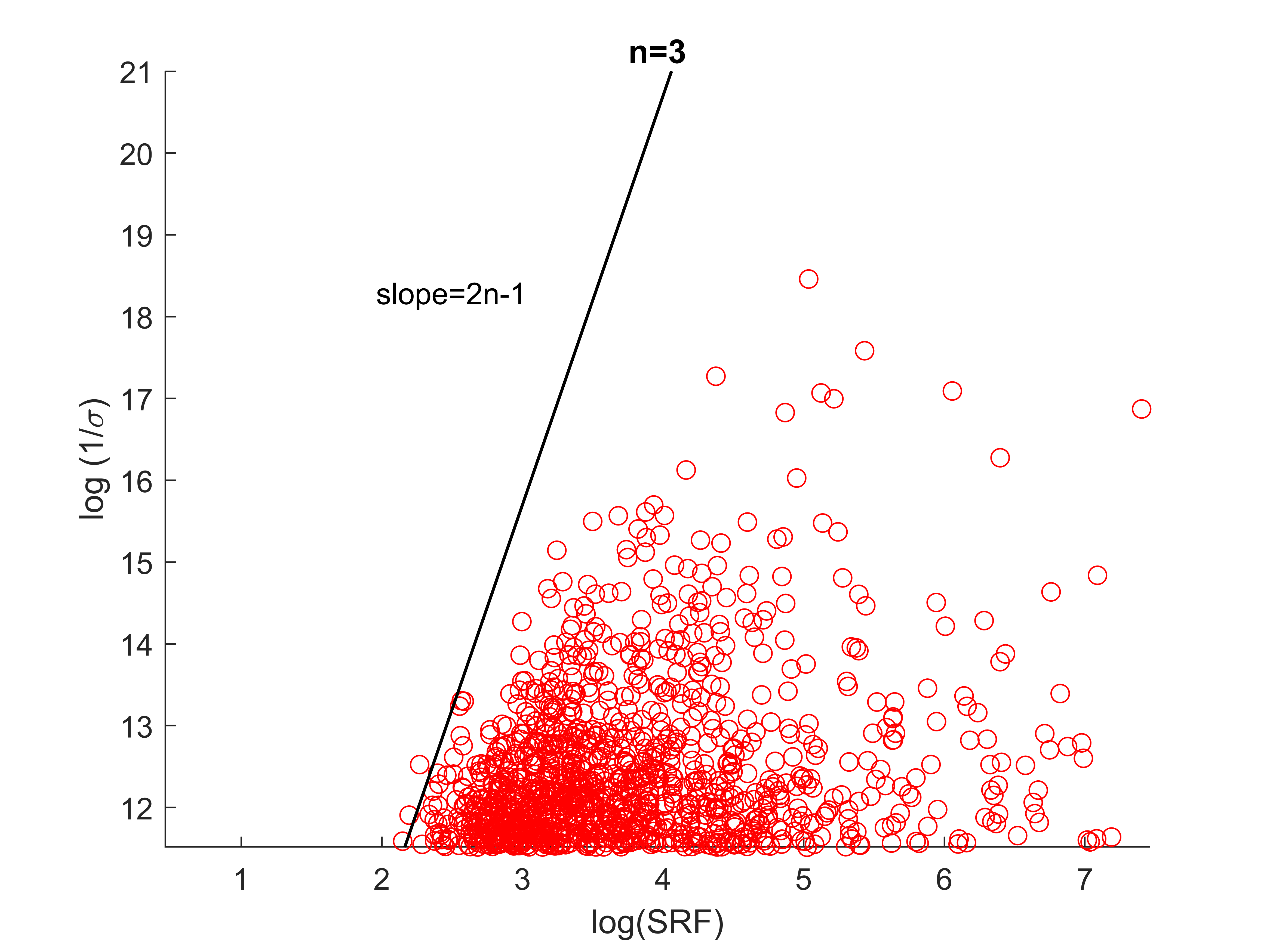
(b) recovery fail

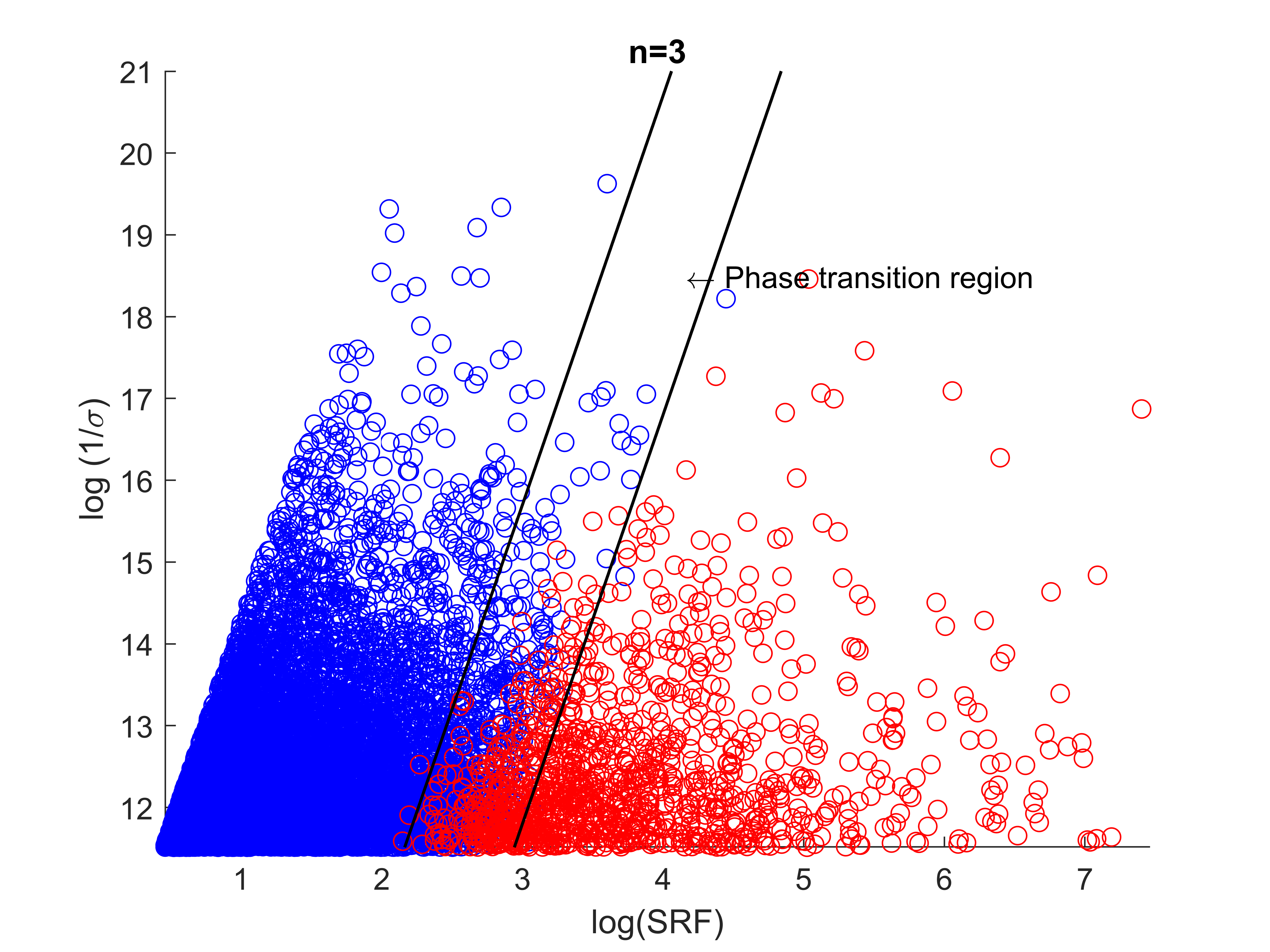
(c) phase transition region

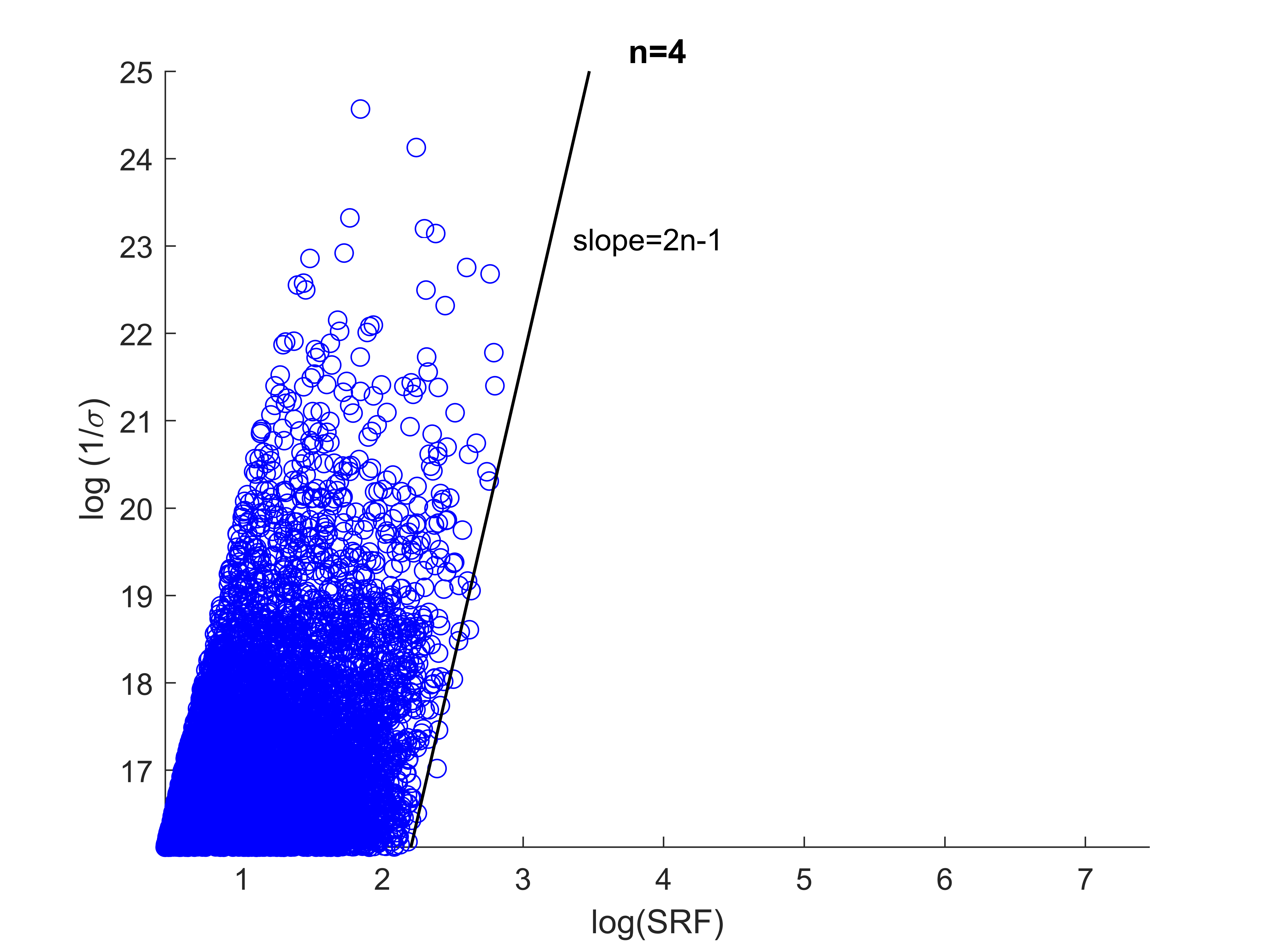
(d) recovery success

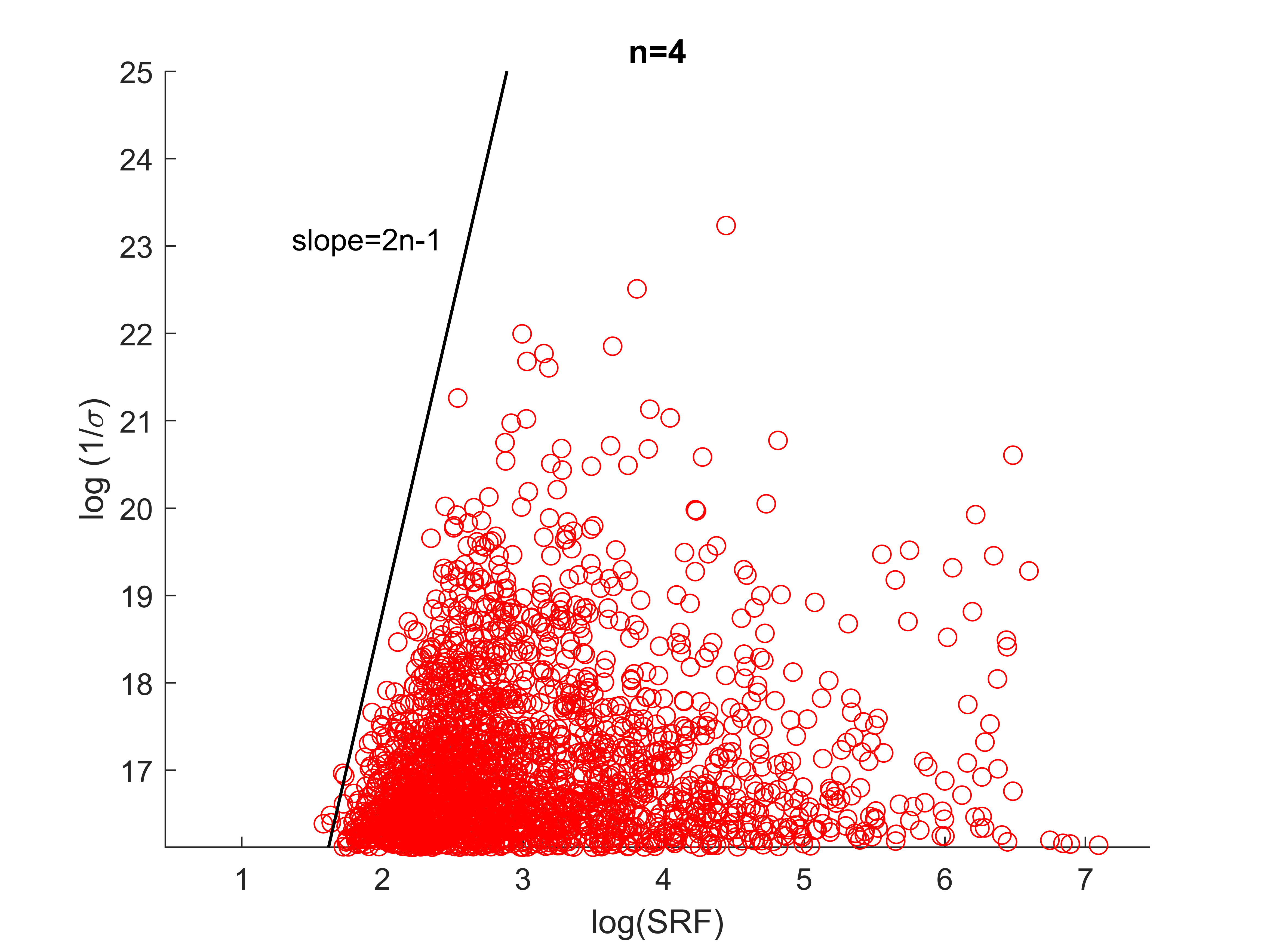
(e) recovery fail

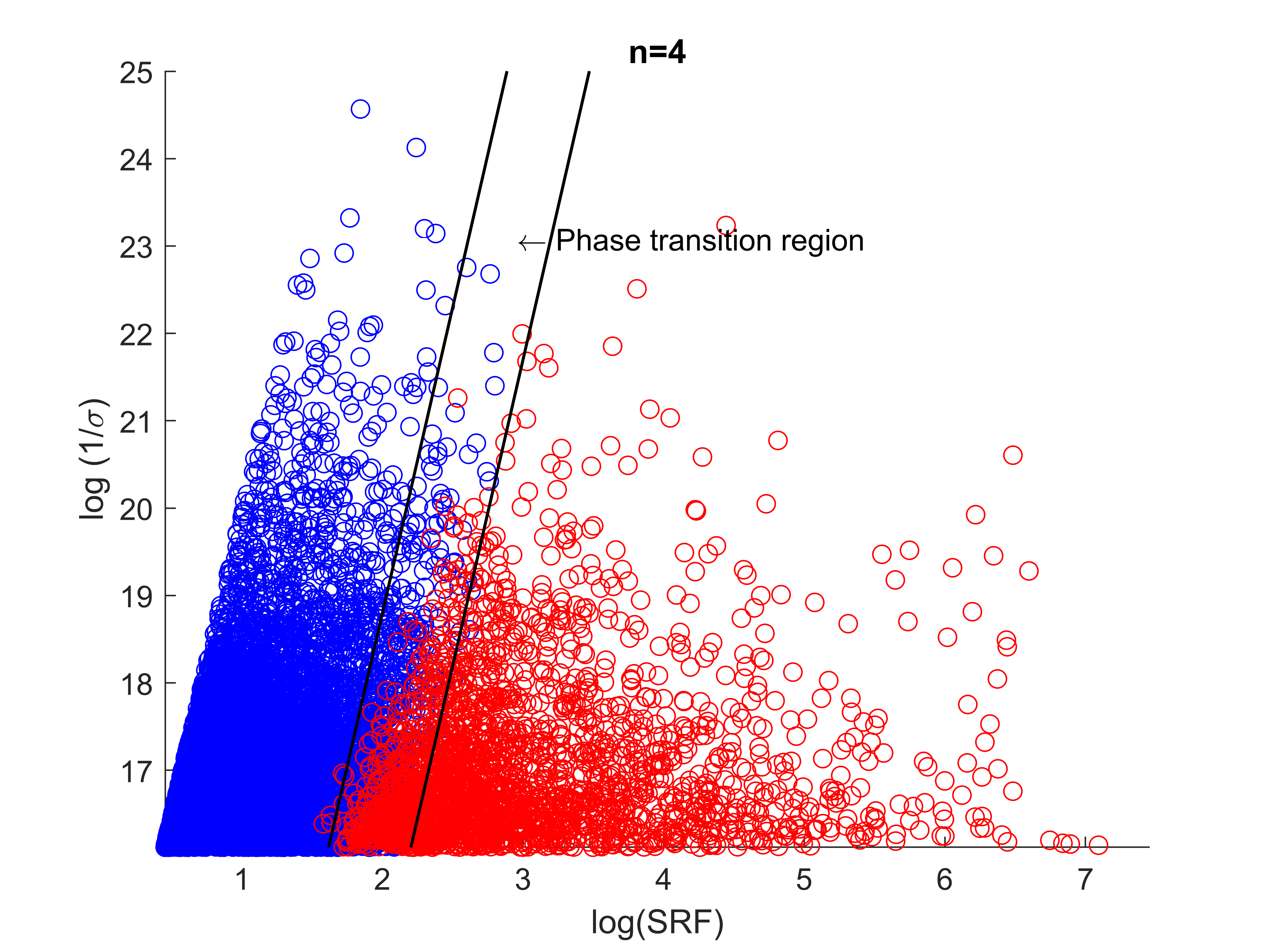
(f) phase transition region

Figure 5.1: Plots of the successful and the unsuccessful support recovery by Algorithm 6 depending on the relation between $\log(SRF)$ and $\log(\frac{1}{\sigma})$. (a) illustrates that locations of three point sources can be stably recovered if $\log(\frac{1}{\sigma})$ is above a line of slope $5$ in the parameter space. Conversely, for the same case, (b) shows that the 2-dimensional support recovery fails if $\log(\frac{1}{\sigma})$ falls below another line of slope $5$. (f) highlights the phase transition region which is bounded by the black slashes in (a) and (b). (d),(e) and (f) illustrate parallel results for four point sources.

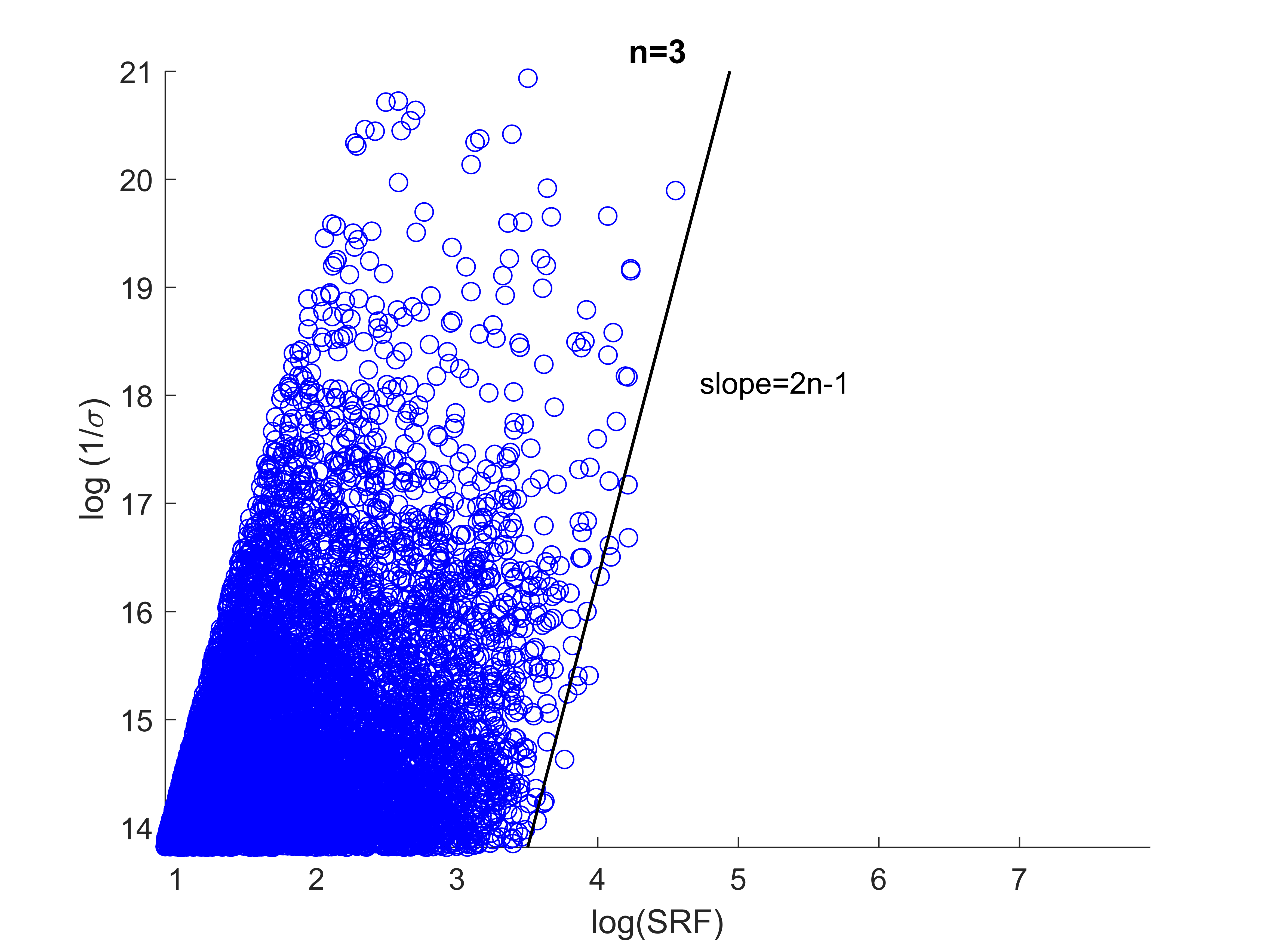
(a) recovery success

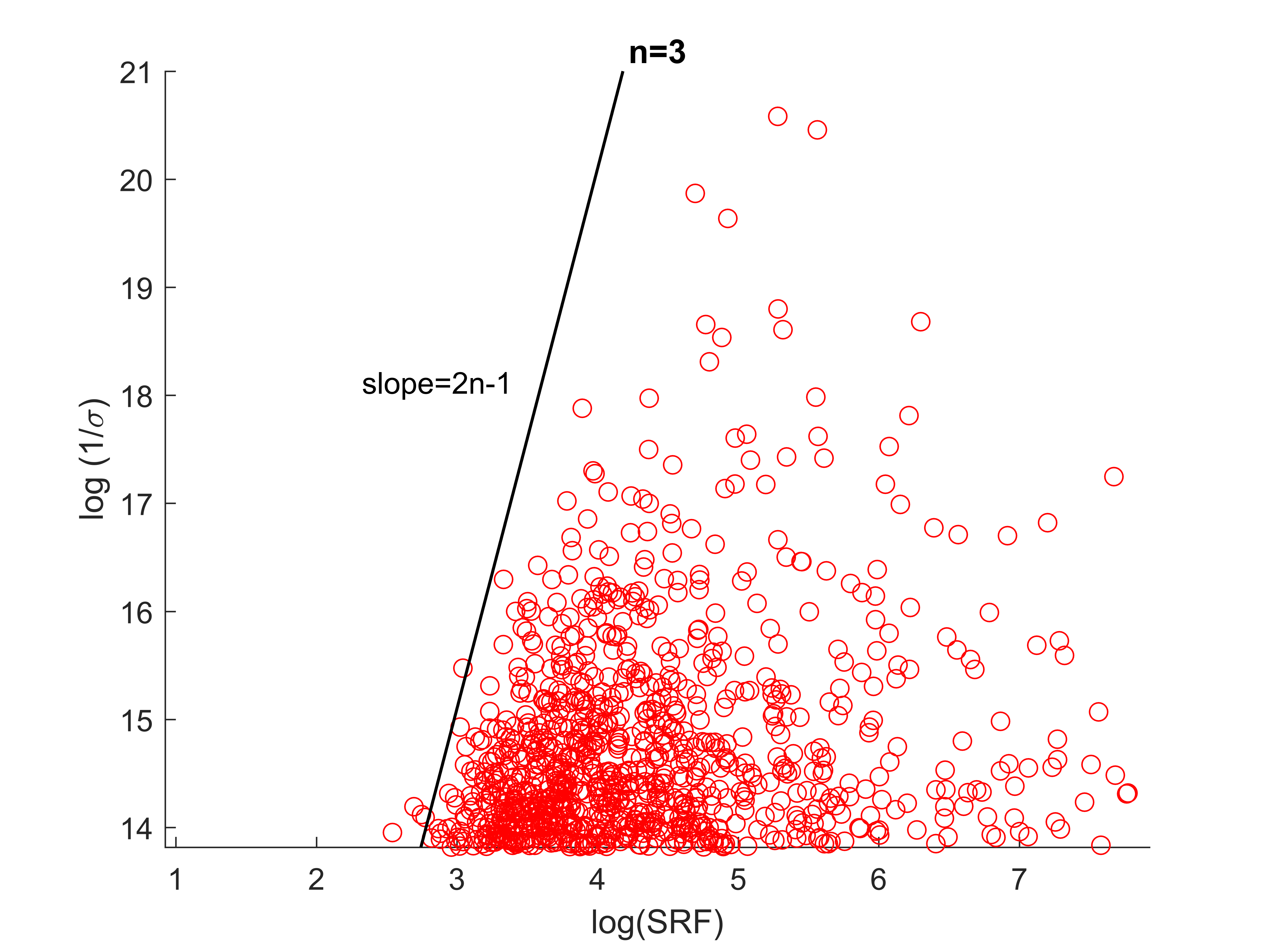
(b) recovery fail

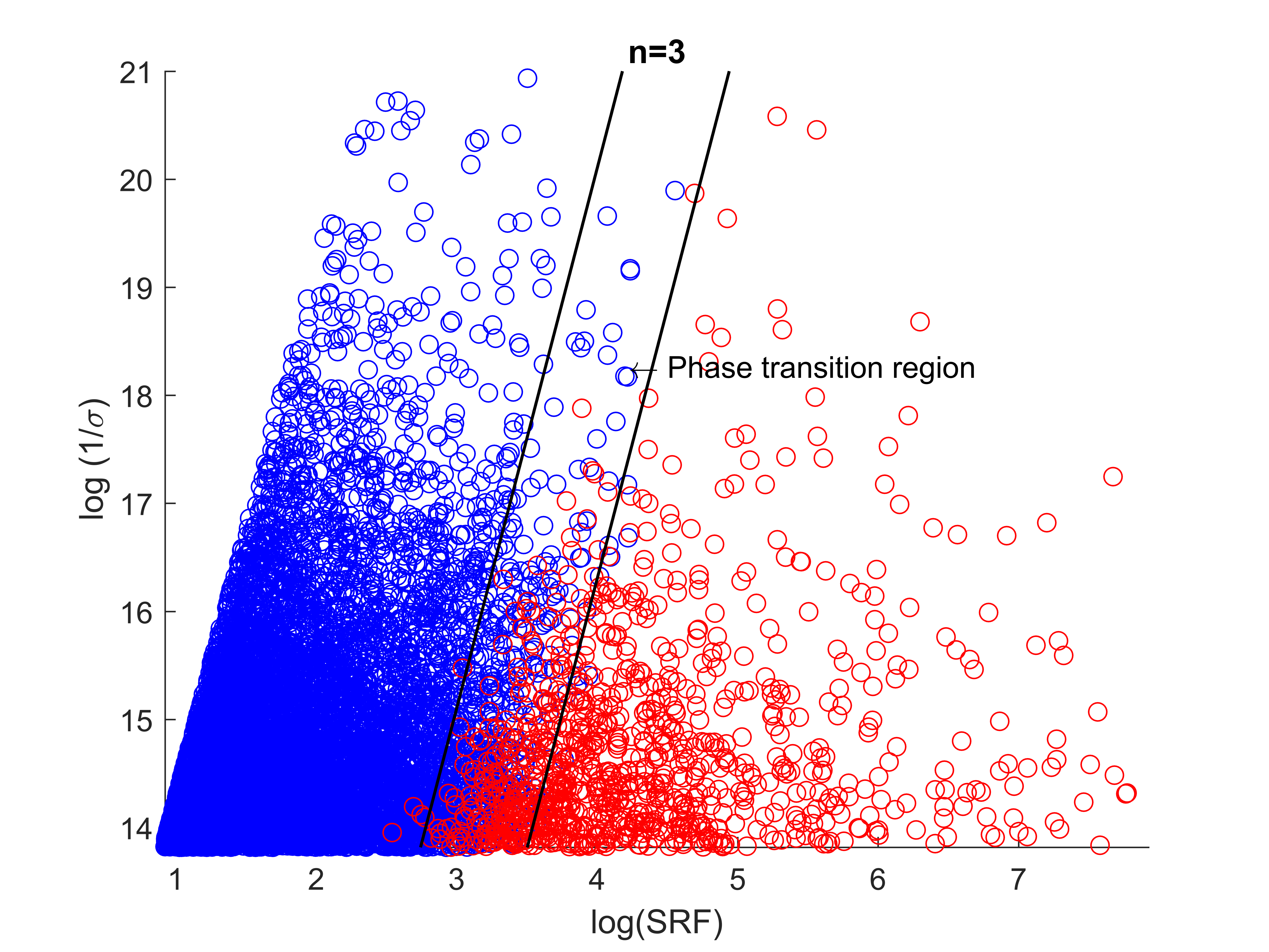
(c) phase transition region

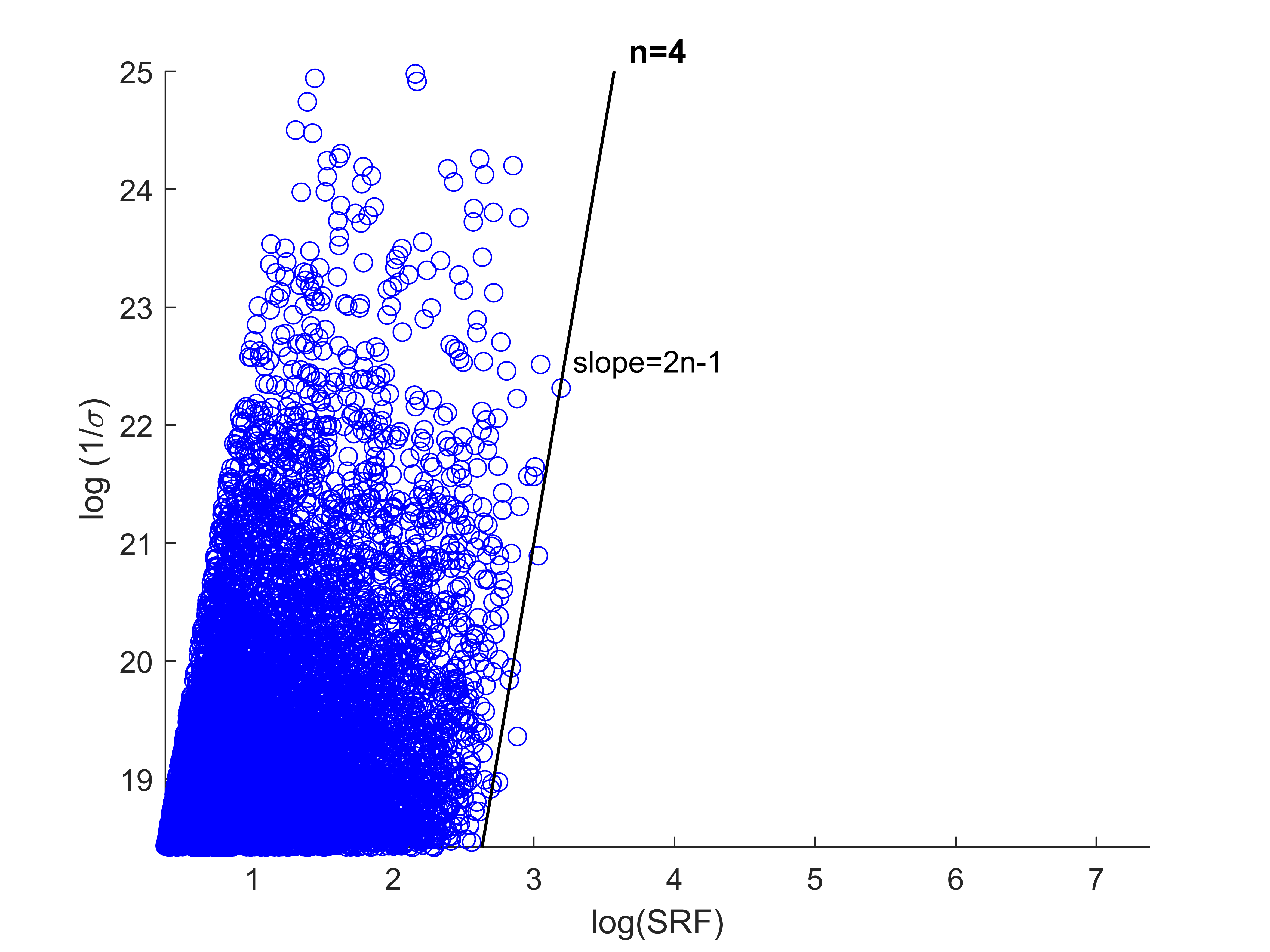
(d) recovery success

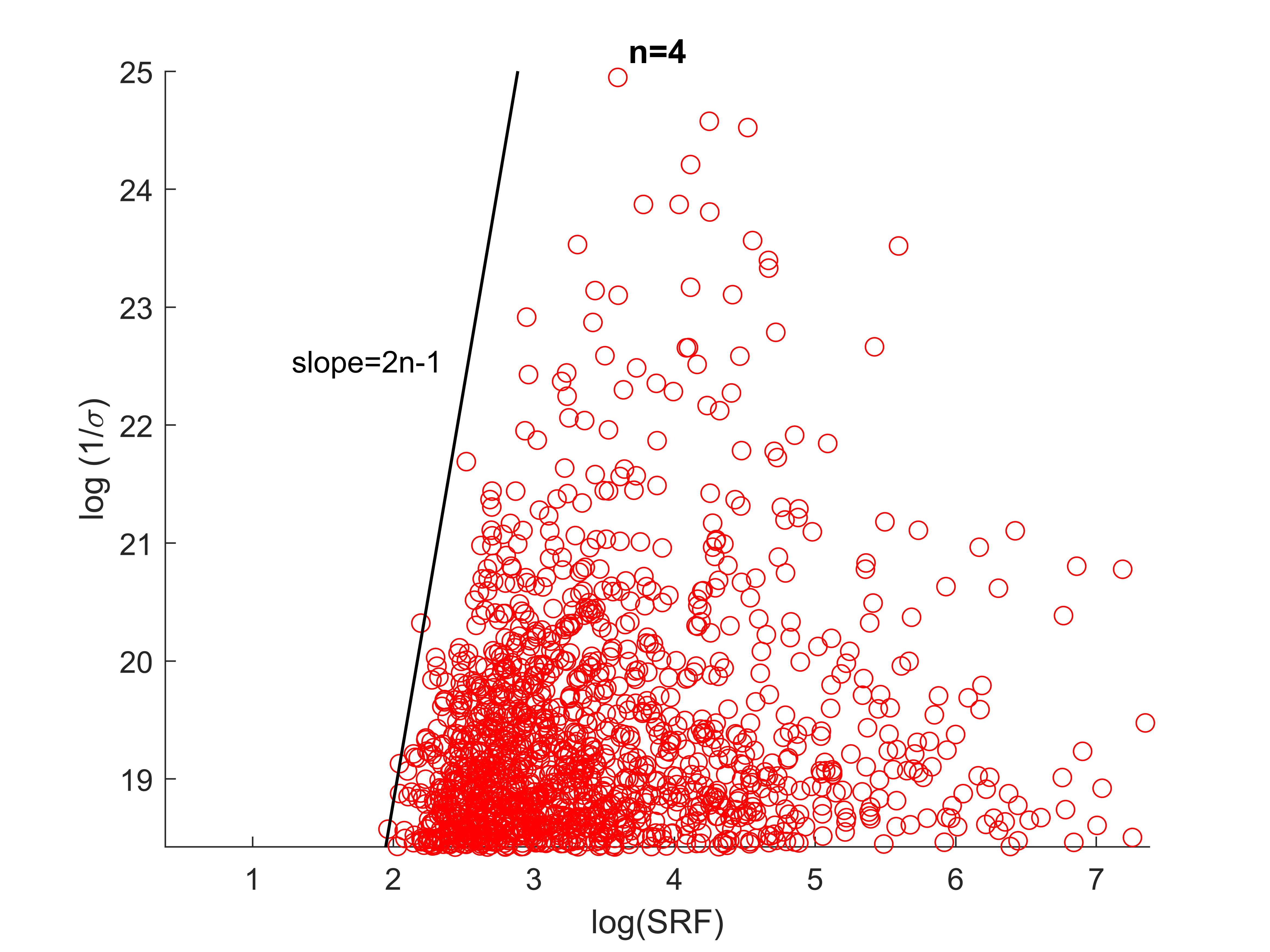
(e) recovery fail

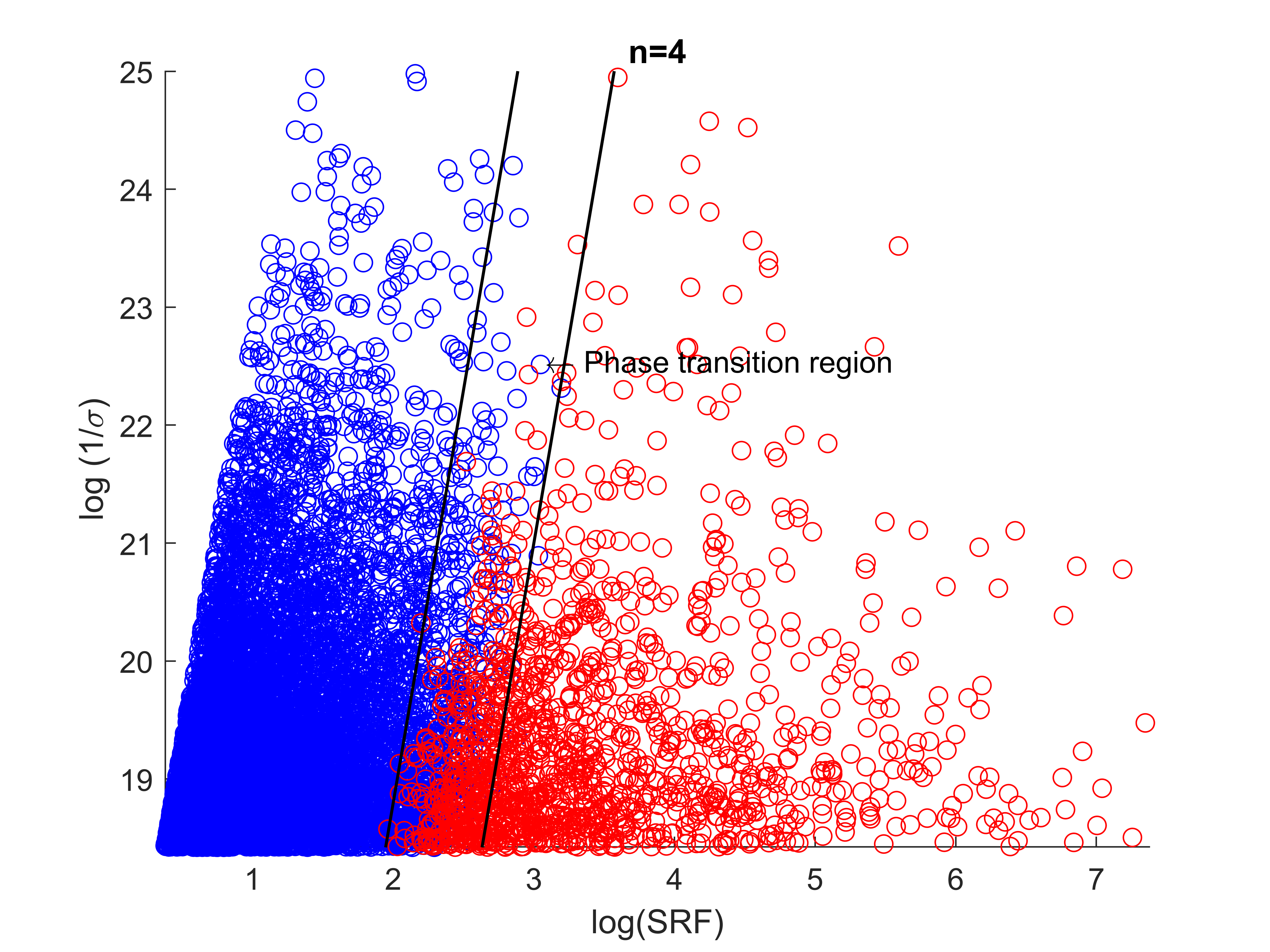
(f) phase transition region

Figure 5.2: Plots of the successful and the unsuccessful support recovery by Algorithm 7 depending on the relation between $\log(SRF)$ and $\log(\frac{1}{\sigma})$. (a) illustrates that locations of three point sources can be stably recovered if $\log(\frac{1}{\sigma})$ is above a line of slope $5$ in the parameter space. Conversely, for the same case, (b) shows that the 3-dimensional support recovery fails if $\log(\frac{1}{\sigma})$ falls below another line of slope $5$. (f) highlights the phase transition region which is bounded by the black slashes in (a) and (b). (d),(e) and (f) illustrate parallel results for four point sources.

6 Appendix

In this section, we present and prove some technical lemmas that are used in the subspace projection strategy we used to prove the main results on the computational resolution limit in multi-dimensions. We denote the unit sphere in $\mathbb{R}^{k}$ as $S_{k-1}$ and its area as $\text{area}(S_{k-1})$. For each $\bm{\mathbf{u}}\in\mathbb{R}^{k}$, we denote

$$N(\bm{\mathbf{u}},\Delta) =\Big{\{}\bm{\mathbf{v}}\Big{|}\bm{\mathbf{v}}\in S_{k-1},||\mathcal{P}_{\bm{\mathbf{v}}^{\perp}}(\bm{\mathbf{u}})||_{2}<||\bm{\mathbf{u}}||_{2}\sin\Delta\Big{\}}.$$ (6.1)

It can be verified that

$$N(\bm{\mathbf{u}},\Delta)=\Big{\{}\bm{\mathbf{v}}\ \Big{|}\bm{\mathbf{v}}\in S_{k-1},|\bm{\mathbf{u}}\cdot\bm{\mathbf{v}}|>||\bm{\mathbf{u}}||_{2}\cos\Delta\Big{\}}.$$

Lemma 6.1.

For $0<\Delta\leq\frac{\pi}{2}$, we have $\text{area}(N(\bm{\mathbf{u}},\Delta))\leq\frac{2\Delta^{k-1}}{k-1}\text{area}(S_{k-2}).$

Proof: WLOG, we consider the case when the unit vector $\bm{\mathbf{u}}=(1,0,\cdots,0)^{T}$. Using spherical coordinates (6.3), the points in $S_{k-1}$ so that $|\bm{\mathbf{u}}\cdot\bm{\mathbf{v}}|>\cos\Delta$ can be expressed by

$$\bm{\mathbf{v}}=(\cos\phi_{1},\ \sin\phi_{1}\cos\phi_{2},\ \cdots,\ \sin\phi_{1}\cdots\sin\phi_{k-2}\cos\phi_{k-1},\ \sin\phi_{1}\cdots\sin\phi_{k-2}\sin\phi_{k-1})^{T}$$

where $0\leq\phi_{1}<\Delta$ or $\pi-\Delta<\phi_{1}\leq\pi$, and $\phi_{2},\cdots,\phi_{k-2}\in[0,\pi],\phi_{k-1}\in[0,2\pi]$. Therefore,

$$\text{area}(N(\bm{\mathbf{u}},\Delta))= 2\int_{0}^{2\pi}\int_{0}^{\pi}\cdots\int_{0}^{\Delta}\sin^{k-2}(\phi_{1})\sin^{k-3}(\phi_{2})\cdots\sin(\phi_{k-1})d\phi_{1}d\phi_{2}\cdots d\phi_{k-2}d\phi_{k-1}$$

$$= 2\text{area}(S_{k-2})\int_{0}^{\Delta}\sin^{k-2}(\phi_{1})d\phi_{1}\leq 2\text{area}(S_{k-2})\int_{0}^{\Delta}\phi_{1}^{k-2}d\phi_{1}=\frac{2\text{area}(S_{k-2})}{k-1}\Delta^{k-1}.$$

Lemma 6.2.

We have the following inequality

$$\frac{(k-1)\text{area}(S_{k-1})}{\text{area}(S_{k-2})}\geq\pi.$$

Proof: It is easy to check the inequality for $k=1,\cdots,5$. For $k\geq 6$, since $\text{area}(S_{k-1})=\frac{2\pi^{\frac{k}{2}}}{\Gamma(\frac{k}{2})}$ where $\Gamma(x)$ is the Gamma function, $\text{area}(S_{k})<\text{area}(S_{k-1})$ when $k>5$. Therefore

$$\frac{\text{area}(S_{k-1})}{\text{area}(S_{k-2})}>\frac{\text{area}(S_{k})}{\text{area}(S_{k-2})}=\frac{2\pi}{k-1}>\frac{\pi}{k-1}$$

where the equality inside follows from a property of the Gamma function. This proves the lemma.

Lemma 6.3.

For $n$ points $\bm{\mathbf{y}}_{j}\in\mathbb{R}^{k},k\geq 2,n\geq 2$, with minimum separation $d_{\min}:=\min_{p\neq j}||\bm{\mathbf{y}}_{p}-\bm{\mathbf{y}}_{j}||_{2}$, let $\Delta=\Big{(}\frac{\pi}{n(n-1)}\Big{)}^{\frac{1}{k-1}}$. There exists an unit vector $\bm{\mathbf{v}}\in\mathbb{R}^{k}$ such that

$$\min_{p\neq j,1\leq p,j\leq n}||\mathcal{P}_{\bm{\mathbf{v}}^{\perp}}(\bm{\mathbf{y}}_{p})-\mathcal{P}_{\bm{\mathbf{v}}^{\perp}}(\bm{\mathbf{y}}_{j})||_{2}\geq\frac{2\Delta d_{\min}}{\pi}.$$ (6.2)

Proof: It is clear that there are at most $\frac{n(n-1)}{2}$ different $\bm{\mathbf{u}}_{pj}=\bm{\mathbf{y}}_{p}-\bm{\mathbf{y}}_{j},p<j$. Using Lemma 6.1 and 6.2, we have

$$\text{area}\left(\cup_{p<j,1\leq j,p\leq n}N(\bm{\mathbf{u}}_{pj},\Delta)\right)\leq\frac{n(n-1)}{2}\frac{2\text{area}(S_{k-2})}{k-1}\Delta^{k-1}\leq\text{area}(S_{k-1}).$$

On the other hand, $\cup_{1\leq j<p\leq n}N(\bm{\mathbf{u}}_{pj},\Delta)$ is an open set in $S_{k-1}$. Thus $S_{k-1}\setminus\cup_{1\leq j<p\leq n}N(\bm{\mathbf{u}}_{pj},\Delta)$ is not empty. By the definition of $N(\bm{\mathbf{u}}_{pj},\Delta)$, there exists an unit vector $\bm{\mathbf{v}}\in\mathbb{R}^{k}$ such that

$$||\mathcal{P}_{\bm{\mathbf{v}}^{\perp}}(\bm{\mathbf{u}}_{pj})||_{2}\geq d_{\min}\sin\Delta,\quad\forall 1\leq p<j\leq n.$$

Finally using the inequality $\sin\Delta\geq\frac{2}{\pi}\Delta$, we obtain (6.2) immediately.

Lemma 6.4.

For $n$ points $\bm{\mathbf{y}}_{j}\in\mathbb{R}^{2},n\geq 2$, with minimum separation $d_{\min}:=\min_{p\neq j}||\bm{\mathbf{y}}_{p}-\bm{\mathbf{y}}_{j}||_{2}$, let $\Delta=\frac{\pi}{n(n+1)}$ and choose $n$ unit vectors $\bm{\mathbf{v}}_{q}=(\cos(2q\Delta),\sin(2q\Delta))^{T}\in\mathbb{R}^{2},q=1,\cdots,\frac{n(n+1)}{2}$. There exists $q^{*}$ so that

$$\min_{p\neq j,1\leq p,j\leq n}||\mathcal{P}_{v_{q^{*}}^{\perp}}(\bm{\mathbf{y}}_{p})-\mathcal{P}_{\bm{\mathbf{v}}_{q^{*}}^{\perp}}(\bm{\mathbf{y}}_{j})||_{2}\geq\frac{2d_{\min}}{n(n+1)}.$$

Proof: It is clear there are at most $\frac{n(n-1)}{2}$ different $\bm{\mathbf{u}}_{pj}=\bm{\mathbf{y}}_{p}-\bm{\mathbf{y}}_{j},1\leq p<j\leq n$. Denote $\bm{\mathbf{v}}(\theta)=(\cos\theta,\sin\theta)^{T}$, we observe that if $||\mathcal{P}_{\bm{\mathbf{v}}(\theta)^{\perp}}(\bm{\mathbf{u}})||_{2}<||\bm{\mathbf{u}}||_{2}\sin\Delta,\theta\in[2\Delta,\pi]$, then $||\mathcal{P}_{\bm{\mathbf{v}}(\theta^{*})^{\perp}}(\bm{\mathbf{u}})||_{2}\geq||\bm{\mathbf{u}}||_{2}\sin\Delta$, for $|\theta^{*}-\theta|\geq 2\Delta,\theta^{*}\in[2\Delta,\pi]$. Therefore, recall definition (6.1), if $\bm{\mathbf{v}}_{q_{0}}\in N(\bm{\mathbf{u}}_{p_{0}j_{0}},\Delta)$ for some $1\leq p_{0},j_{0}\leq n$, then $\bm{\mathbf{v}}_{q}\not\in N(\bm{\mathbf{u}}_{p_{0}j_{0}},\Delta),\forall q\neq q_{0},q=1,\cdots,\frac{n(n+1)}{2}$. Since we have $\frac{n(n+1)}{2}$ different $q$’s, there must be some $\bm{\mathbf{v}}_{q^{*}}\not\in\cup_{p<j,1\leq j,p\leq n}N(\bm{\mathbf{u}}_{pj},\Delta)$. Hence,

$$\min_{p\neq j,1\leq p,j\leq n}||\mathcal{P}_{\bm{\mathbf{v}}_{q^{*}}^{\perp}}(\bm{\mathbf{y}}_{p})-\mathcal{P}_{\bm{\mathbf{v}}_{q^{*}}^{\perp}}(\bm{\mathbf{y}}_{j})||_{2}\geq d_{\min}\sin\Delta\geq d_{\min}\frac{2\Delta}{\pi},$$

whence the lemma follows.

We next present a lemmas that is used to prove the results for support recovery. We consider the unit sphere in $\mathbb{R}^{k}$ and the following spherical coordinate

$$x_{1}(\Phi) =\cos(\phi_{1})$$ (6.3)

$$x_{2}(\Phi) =\sin(\phi_{1})\cos(\phi_{2})$$

$$\vdots$$

$$x_{k-1}(\Phi) =\sin(\phi_{1})\cdots\sin(\phi_{k-2})\cos(\phi_{k-1})$$

$$x_{k}(\Phi) =\sin(\phi_{1})\cdots\sin(\phi_{k-2})\sin(\phi_{k-1}),$$

where $\Phi=(\phi_{1},\cdots,\phi_{k-1})\in[0,\pi]^{k-2}\times[0,2\pi)$. For $0<\theta<\frac{\pi}{2}$ and $N=\lfloor\frac{\pi}{2\theta}\rfloor$, we denote

$$\bm{\mathbf{v}}_{\tau_{1}\cdots\tau_{k-1}}=\big{(}x_{1}(\Phi_{\tau_{1}\cdots\tau_{k-1}}),\cdots,x_{k}(\Phi_{\tau_{1}\cdots\tau_{k-1}})\big{)}^{T},\quad 1\leq\tau_{j}\leq N,$$ (6.4)

where $\Phi_{\tau_{1}\cdots\tau_{k-1}}=(\tau_{1}\theta,\cdots,\tau_{k-1}\theta)$. It is obvious that $\Phi_{\tau_{1}\cdots\tau_{k-1}}\in[0,\frac{\pi}{2}]^{k-1}$ and $\bm{\mathbf{v}}_{\tau_{1}\cdots\tau_{k-1}}\neq\bm{\mathbf{v}}_{p_{1}\cdots p_{k-1}}$ if $(\tau_{1},\cdots,\tau_{k-1})\neq(p_{1},\cdots,p_{k-1})$. There are $N^{k-1}$ different unit vectors of the form (6.4).

Lemma 6.5.

For two different vectors $\bm{\mathbf{v}}_{\tau_{1}\cdots\tau_{k-1}}\neq\bm{\mathbf{v}}_{p_{1}\cdots p_{k-1}}$ in (6.4), we have

$$0\leq\bm{\mathbf{v}}_{\tau_{1}\cdots\tau_{k-1}}\cdot\bm{\mathbf{v}}_{p_{1}\cdots p_{k-1}}\leq\cos\theta.$$ (6.5)

Proof: Because $\sin\tau_{j}\theta\geq 0,\cos\tau_{j}\theta\geq 0$, for $\tau_{j}$ in (6.4), the first inequality, $0\leq\bm{\mathbf{v}}_{\tau_{1}\cdots\tau_{k-1}}\cdot\bm{\mathbf{v}}_{p_{1}\cdots p_{k-1}}$, is easy to verify using (6.3). We next prove $\bm{\mathbf{v}}_{\tau_{1}\cdots\tau_{k-1}}\cdot\bm{\mathbf{v}}_{p_{1}\cdots p_{k-1}}\leq\cos\theta$ by induction. When $k=2$, it is clear that (6.5) holds. Suppose when $k=j-1$, (6.5) holds. For $k=j$, we consider the inner product between the vector $\bm{\mathbf{v}}_{\tau_{1}\cdots\tau_{j-2}\tau_{j-1}}$ and $\bm{\mathbf{v}}_{p_{1}\cdots p_{j-2}p_{j-1}}$. We first observe that (using (6.3)), we have

$$\bm{\mathbf{v}}_{\tau_{1}\cdots\tau_{j-2}\tau_{j-1}}\cdot\bm{\mathbf{v}}_{p_{1}\cdots p_{j-2}\tau_{j-1}}=\bm{\mathbf{v}}_{\tau_{1}\cdots\tau_{j-2}}\cdot\bm{\mathbf{v}}_{p_{1}\cdots p_{j-2}},$$

where $\bm{\mathbf{v}}_{p_{1}\cdots p_{j-2}\tau_{j-1}}$ is an unit vector in $\mathbb{R}^{j}$ and $\bm{\mathbf{v}}_{\tau_{1}\cdots\tau_{j-2}},\bm{\mathbf{v}}_{p_{1}\cdots p_{j-2}}$ a unit vector in $\mathbb{R}^{j-1}$. By the assumption that (6.5) holds for $k=j-1$, the above equality gives

$$0\leq\bm{\mathbf{v}}_{\tau_{1}\cdots\tau_{j-2}\tau_{j-1}}\cdot\bm{\mathbf{v}}_{p_{1}\cdots p_{j-2}\tau_{j-1}}\leq\cos\theta.$$ (6.6)

We then prove $\bm{\mathbf{v}}_{\tau_{1}\cdots\tau_{j-2}\tau_{j-1}}\cdot\bm{\mathbf{v}}_{p_{1}\cdots p_{j-2}p_{j-1}}\leq\cos\theta$. Using the decomposition

$$\bm{\mathbf{v}}_{p_{1}\cdots p_{j-2}p_{j-1}}=\bm{\mathbf{v}}_{p_{1}\cdots p_{j-2}\tau_{j-1}}+\bm{\mathbf{x}},$$

where

$$\bm{\mathbf{x}}=\sin(\tau_{1}\theta)\sin(p_{1}\theta)\cdots\sin(\tau_{j-2}\theta)\sin(p_{j-2}\theta)\big{(}0,\cdots,0,\cos(p_{j-1}\theta)-\cos(\tau_{j-1}\theta),\sin(p_{j-1}\theta)-\sin(\tau_{j-1}\theta)\big{)}^{T},$$

we have

$$\bm{\mathbf{v}}_{\tau_{1}\cdots\tau_{j-1}}\cdot\bm{\mathbf{v}}_{p_{1}\cdots p_{j-1}}=\bm{\mathbf{v}}_{\tau_{1}\cdots\tau_{j-2}\tau_{j-1}}\cdot(\bm{\mathbf{v}}_{p_{1}\cdots p_{j-2}\tau_{j-1}}+\bm{\mathbf{x}})$$

$$= \bm{\mathbf{v}}_{\tau_{1}\cdots\tau_{j-2}\tau_{j-1}}\cdot\bm{\mathbf{v}}_{p_{1}\cdots p_{j-2}\tau_{j-1}}+\bm{\mathbf{v}}_{\tau_{1}\cdots\tau_{j-2}\tau_{j-1}}\cdot\bm{\mathbf{x}}$$

$$\leq \cos\theta+\bm{\mathbf{v}}_{\tau_{1}\cdots\tau_{j-2}\tau_{j-1}}\cdot\bm{\mathbf{x}}\quad(\text{by (\ref{equ:projectlemangle2})})$$

$$\leq \cos\theta+\sin(\tau_{1}\theta)\sin(p_{1}\theta)\cdots\sin(\tau_{j-2}\theta)\sin(p_{j-2}\theta)\cos(\tau_{j-1}\theta)\big{(}\cos(p_{j-1}\theta)-\cos(\tau_{j-1}\theta)\big{)}$$

$$+\sin(\tau_{1}\theta)\sin(p_{1}\theta)\cdots\sin(\tau_{j-2}\theta)\sin(p_{j-2}\theta)\sin(\tau_{j-1}\theta)\big{(}\sin(p_{j-1}\theta)-\sin({\tau_{j-1}}\theta)\big{)}$$

$$= \cos\theta+\sin(\tau_{1}\theta)\sin(p_{1}\theta)\cdots\sin(\tau_{j-2}\theta)\sin(p_{j-2}\theta)\big{(}\cos(\tau_{j-1}\theta)\cos(p_{j-1}\theta)+\sin(\tau_{j-1}\theta)\sin(p_{j-1}\theta)-1\big{)}$$

$$\leq \cos\theta.$$

This completes the induction argument and proves the lemma.

Lemma 6.6.

For a vector $\bm{\mathbf{u}}\in\mathbb{R}^{k}$, suppose $||\mathcal{P}_{\bm{\mathbf{v}}_{\tau_{1}\cdots\tau_{k-1}}^{\perp}}(\bm{\mathbf{u}})||_{2}<\sin(\frac{\theta}{2})||\bm{\mathbf{u}}||_{2}$ with $\bm{\mathbf{v}}_{\tau_{1}\cdots\tau_{k-1}}$ defined in (6.4), we have $||\mathcal{P}_{\bm{\mathbf{v}}_{p_{1}\cdots p_{k-1}}^{\perp}}(\bm{\mathbf{u}})||_{2}\geq\sin(\frac{\theta}{2})||\bm{\mathbf{u}}||_{2}$ for $\bm{\mathbf{v}}_{p_{1}\cdots p_{k-1}}\neq\bm{\mathbf{v}}_{\tau_{1}\cdots\tau_{k-1}}$.

Proof: We denote the $2$-dimensional space spanned by $\bm{\mathbf{v}}_{\tau_{1}\cdots\tau_{k-1}}$ and $\bm{\mathbf{v}}_{p_{1}\cdots p_{k-1}}$ by $S$. We decompose $\bm{\mathbf{u}}$ as $\bm{\mathbf{u}}=\bm{\mathbf{u}}_{S}+\bm{\mathbf{u}}_{S^{\perp}}$. The condition $||\mathcal{P}_{\bm{\mathbf{v}}_{\tau_{1}\cdots\tau_{k-1}}^{\perp}}(\bm{\mathbf{u}})||_{2}<\sin(\frac{\theta}{2})||\bm{\mathbf{u}}||_{2}$ implies that

$$||\mathcal{P}_{\bm{\mathbf{v}}_{\tau_{1}\cdots\tau_{k-1}}^{\perp}}(\bm{\mathbf{u}})||_{2}^{2}=||\bm{\mathbf{u}}_{S^{\perp}}||_{2}^{2}+||\bm{\mathbf{u}}_{S}-\big{(}\bm{\mathbf{u}}_{S}\cdot\bm{\mathbf{v}}_{\tau_{1}\cdots\tau_{k-1}}\big{)}\bm{\mathbf{v}}_{\tau_{1}\cdots\tau_{k-1}}||_{2}^{2}<\sin(\frac{\theta}{2})^{2}||\bm{\mathbf{u}}||_{2}^{2}.$$

Using the decomposition $\sin(\frac{\theta}{2})^{2}||\bm{\mathbf{u}}||_{2}^{2}=\sin(\frac{\theta}{2})^{2}(||\bm{\mathbf{u}}_{S}||_{2}^{2}+||\bm{\mathbf{u}}_{S^{\perp}}||_{2}^{2})$, we further get

$$||\bm{\mathbf{u}}_{S}-\big{(}\bm{\mathbf{u}}_{S}\cdot\bm{\mathbf{v}}_{\tau_{1}\cdots\tau_{k-1}}\big{)}\bm{\mathbf{v}}_{\tau_{1}\cdots\tau_{k-1}}||_{2}^{2}<\sin(\frac{\theta}{2})^{2}||\bm{\mathbf{u}}_{S}||_{2}^{2}.$$

It follows that

$$||\bm{\mathbf{u}}_{S}||_{2}^{2}-|\bm{\mathbf{u}}_{S}\cdot\bm{\mathbf{v}}_{\tau_{1}\cdots\tau_{k-1}}|^{2}=||\bm{\mathbf{u}}_{S}-\big{(}\bm{\mathbf{u}}_{S}\cdot\bm{\mathbf{v}}_{\tau_{1}\cdots\tau_{k-1}}\big{)}\bm{\mathbf{v}}_{\tau_{1}\cdots\tau_{k-1}}||_{2}^{2}<\sin(\frac{\theta}{2})^{2}||\bm{\mathbf{u}}_{S}||_{2}^{2}.$$

Therefore, $|\bm{\mathbf{u}}_{S}\cdot\bm{\mathbf{v}}_{\tau_{1}\cdots\tau_{k-1}}|^{2}>\cos(\frac{\theta}{2})^{2}||\bm{\mathbf{u}}_{S}||_{2}^{2}$. Denoting the angle between $\bm{\mathbf{v}}_{\tau_{1}\cdots\tau_{k-1}}$ and $\bm{\mathbf{u}}_{S}$ by $\angle(\bm{\mathbf{v}}_{\tau_{1}\cdots\tau_{k-1}},\bm{\mathbf{u}}_{S})$, we thus have $\angle(\bm{\mathbf{v}}_{\tau_{1}\cdots\tau_{k-1}},\bm{\mathbf{u}}_{S})<\frac{\theta}{2}$. On the hand, by Lemma 6.5, $0\leq\bm{\mathbf{v}}_{\tau_{1}\cdots\tau_{k-1}}\cdot\bm{\mathbf{v}}_{p_{1}\cdots p_{k-1}}\leq\cos\theta$ and this gives $\theta\leq\angle(\bm{\mathbf{v}}_{\tau_{1}\cdots\tau_{k-1}},\bm{\mathbf{v}}_{p_{1}\cdots p_{k-1}})\leq\frac{\pi}{2}$. Combining these estimates, we have

$$\frac{\theta}{2}\leq\angle(\bm{\mathbf{v}}_{p_{1}\cdots p_{k-1}},\bm{\mathbf{u}}_{S})\leq\frac{\pi}{2}+\frac{\theta}{2}.$$

Note that $\frac{\theta}{2}<\frac{\pi}{4}$, we can further get

$$|\bm{\mathbf{u}}_{S}\cdot\bm{\mathbf{v}}_{p_{1}\cdots p_{k-1}}|\leq\cos(\frac{\theta}{2})||\bm{\mathbf{u}}_{S}||_{2}.$$

As a consequence,

$$||\mathcal{P}_{\bm{\mathbf{v}}_{p_{1}\cdots p_{k-1}}^{\perp}}(\bm{\mathbf{u}})||_{2}^{2}=||\bm{\mathbf{u}}_{S^{\perp}}||_{2}^{2}+||\bm{\mathbf{u}}_{S}-\big{(}\bm{\mathbf{u}}_{S}\cdot\bm{\mathbf{v}}_{p_{1}\cdots p_{k-1}}\big{)}\bm{\mathbf{v}}_{p_{1}\cdots p_{k-1}}||_{2}^{2}\geq||\bm{\mathbf{u}}_{S^{\perp}}||_{2}^{2}+\sin(\frac{\theta}{2})^{2}||\bm{\mathbf{u}}_{S}||_{2}^{2}\geq\sin(\frac{\theta}{2})^{2}||\bm{\mathbf{u}}||_{2}^{2}.$$

This completes the proof.

Lemma 6.7.

Let $\bm{\mathbf{y}}_{1},\bm{\mathbf{y}}_{2},\cdots,\bm{\mathbf{y}}_{n}$ be $n$ different points in $\mathbb{R}^{k}$, $k\geq 2$. Let  $d_{\min}=\min_{p\neq j}||\bm{\mathbf{y}}_{p}-\bm{\mathbf{y}}_{j}||_{2}$ and $\Delta=\frac{\pi}{8}(\frac{2}{(n+2)(n-1)})^{\frac{1}{k-1}}$. Then there exist $n+1$ unit vectors $\bm{\mathbf{v}}_{q}$’s such that $0\leq\bm{\mathbf{v}}_{p}\cdot\bm{\mathbf{v}}_{j}\leq\cos 2\Delta$ for $p\neq j$ and

$$\min_{p\neq j,1\leq p,j\leq n}||\mathcal{P}_{\bm{\mathbf{v}}_{q}^{\perp}}(\bm{\mathbf{y}}_{p})-\mathcal{P}_{\bm{\mathbf{v}}_{q}^{\perp}}(\bm{\mathbf{y}}_{j})||_{2}\geq\frac{2\Delta d_{\min}}{\pi},\quad q=1,\cdots,n+1.$$ (6.7)

Proof: Note that there are at most $\frac{n(n-1)}{2}$ different vectors of the form $\bm{\mathbf{u}}_{pj}=\bm{\mathbf{y}}_{p}-\bm{\mathbf{y}}_{j},p<j$. For each $\bm{\mathbf{u}}_{pj}$, consider the set $N(\bm{\mathbf{u}}_{pj},\Delta)$ defined in (6.1). Let $\theta=2\Delta$ and introduce the vectors $\bm{\mathbf{v}}_{\tau_{1}\cdots\tau_{k-1}}$ as in (6.4). Using Lemma 6.6, we can derive that each set $N(\bm{\mathbf{u}}_{pj},\Delta)$ contains at most one of the vectors $\bm{\mathbf{v}}_{\tau_{1}\cdots\tau_{k-1}}$’s. As a result, $\cup_{p<j,1\leq j,p\leq n}N(\bm{\mathbf{u}}_{pj},\Delta)$ contains at most $\frac{n(n-1)}{2}$ vectors of the form $\bm{\mathbf{v}}_{\tau_{1}\cdots\tau_{k-1}}$.

Next recall that there are $N^{k-1}$ different vectors of the form in (6.4), where $N=\lfloor\frac{\pi}{2\theta}\rfloor\geq\frac{\pi}{2\theta}-1$. Since

$$\theta=2\Delta=\frac{\pi}{4}(\frac{2}{(n+2)(n-1)})^{\frac{1}{k-1}},$$

we have

$$N^{k-1}\geq\Big{(}\frac{\pi}{2\theta}-1\Big{)}^{k-1}=\Big{(}2(\frac{(n+2)(n-1)}{2})^{\frac{1}{k-1}}-1\Big{)}^{k-1}\geq\Big{(}(\frac{(n+2)(n-1)}{2})^{\frac{1}{k-1}}\Big{)}^{k-1}=\frac{(n+2)(n-1)}{2}.$$

Note that $\frac{(n+2)(n-1)}{2}-\frac{n(n-1)}{2}=n+1$, we can find $n+1$ vectors of the form $\bm{\mathbf{v}}_{\tau_{1}\cdots\tau_{k-1}}$ that are not contained in the set $\cup_{p<j,1\leq j,p\leq n}N(\bm{\mathbf{u}}_{pj},\Delta)$. That is, we can find $n+1$ unit vectors, say, $\bm{\mathbf{v}}_{q}$, $1\leq q\leq n+1$, which satisfy (6.7). Moreover, by Lemma 6.5, these vectors also satisfy the condition that $0\leq\bm{\mathbf{v}}_{p}\cdot\bm{\mathbf{v}}_{j}\leq\cos 2\Delta$ for $p\neq j$. This completes the proof.

Lemma 6.8.

Let $k\geq 2$. For a vector $\bm{\mathbf{u}}\in\mathbb{R}^{k}$, and two unit vectors $\bm{\mathbf{v}}_{1},\bm{\mathbf{v}}_{2}\in\mathbb{R}^{k}$ satisfying $0\leq\bm{\mathbf{v}}_{1}\cdot\bm{\mathbf{v}}_{2}\leq\cos\theta$, we have

$$||\mathcal{P}_{\bm{\mathbf{v}}_{1}^{\perp}}(\bm{\mathbf{u}})||_{2}^{2}+||\mathcal{P}_{\bm{\mathbf{v}}_{2}^{\perp}}(\bm{\mathbf{u}})||_{2}^{2}\geq(1-\cos(\theta))||\bm{\mathbf{u}}||_{2}^{2}.$$ (6.8)

Proof: We first prove the lemma for dimension two. Indeed, for $\bm{\mathbf{u}}\in\mathbb{R}^{2}$, and two unit vectors $\bm{\mathbf{v}}_{1},\bm{\mathbf{v}}_{2}\in\mathbb{R}^{2}$ satisfying $0\leq\bm{\mathbf{v}}_{1}\cdot\bm{\mathbf{v}}_{2}\leq\cos\theta$, we have

$$\Big{|}\Big{|}{(\bm{\mathbf{v}}_{1}\cdot\bm{\mathbf{u}},\ \bm{\mathbf{v}}_{2}\cdot\bm{\mathbf{u}})^{T}}\Big{|}\Big{|}_{2}^{2}=\Big{|}\Big{|}{\begin{pmatrix}\bm{\mathbf{v}}_{1}^{T}\\ \bm{\mathbf{v}}_{2}^{T}\end{pmatrix}\cdot\bm{\mathbf{u}}}\Big{|}\Big{|}_{2}^{2}\geq\sigma_{\min}^{2}(\begin{pmatrix}\bm{\mathbf{v}}_{1}^{T}\\ \bm{\mathbf{v}}_{2}^{T}\end{pmatrix})||\bm{\mathbf{u}}||_{2}^{2}\geq(1-\cos\theta)||\bm{\mathbf{u}}||_{2}^{2},$$ (6.9)

where the last inequality follows from calculating $\sigma_{\min}(\begin{pmatrix}\bm{\mathbf{v}}_{1}^{T}\\ \bm{\mathbf{v}}_{2}^{T}\end{pmatrix})$. We now prove the lemma for $k$ dimensional case. When $\cos\theta=1$, the lemma obviously holds. When $\cos\theta<1$, we denote the $2$-dimensional space spanned by $\bm{\mathbf{v}}_{1}$ and $\bm{\mathbf{v}}_{2}$ as $S$. Let $\bm{\mathbf{g}}_{1}$ and $\bm{\mathbf{g}}_{2}$ be the unit vectors in $S$ that are perpendicular to $\bm{\mathbf{v}}_{1}$ and $\bm{\mathbf{v}}_{2}$ respectively and satisfy $0\leq\bm{\mathbf{g}}_{1}\cdot\bm{\mathbf{g}}_{2}\leq\cos\theta$ as well. Then $\bm{\mathbf{u}}$ has the decomposition

$$\bm{\mathbf{u}}=\mathcal{P}_{S^{\perp}}(\bm{\mathbf{u}})+\lambda_{j}\bm{\mathbf{g}}_{j}+\eta_{j}\bm{\mathbf{v}}_{j},\quad j=1,2,$$

where $\lambda_{j}=\mathcal{P}_{S}(\bm{\mathbf{u}})\cdot\bm{\mathbf{g}}_{j}$ and $\eta_{j}=\mathcal{P}_{S}(\bm{\mathbf{u}})\cdot\bm{\mathbf{v}}_{j}$. Since $S$ is a 2-dimensional subspace, applying (6.9) in $S$, we have $||(\lambda_{1},\lambda_{2})^{T}||_{2}^{2}=||(\mathcal{P}_{S}(\bm{\mathbf{u}})\cdot\bm{\mathbf{g}}_{1},\mathcal{P}_{S}(\bm{\mathbf{u}})\cdot\bm{\mathbf{g}}_{2})^{T}||_{2}^{2}\geq(1-\cos\theta)||\mathcal{P}_{S}(\bm{\mathbf{u}})||_{2}^{2}$. Note that $\mathcal{P}_{\bm{\mathbf{v}}_{j}^{\perp}}(\bm{\mathbf{u}})=\mathcal{P}_{S^{\perp}}(\bm{\mathbf{u}})+\lambda_{j}\bm{\mathbf{g}}_{j},j=1,2$, we further have

$$||\mathcal{P}_{\bm{\mathbf{v}}_{1}^{\perp}}(\bm{\mathbf{u}})||_{2}^{2}+||\mathcal{P}_{\bm{\mathbf{v}}_{2}^{\perp}}(\bm{\mathbf{u}})||_{2}^{2}=2||\mathcal{P}_{S^{\perp}}(\bm{\mathbf{u}})||_{2}^{2}+\lambda_{1}^{2}+\lambda_{2}^{2}$$

$$\geq 2||\mathcal{P}_{S^{\perp}}(\bm{\mathbf{u}})||_{2}^{2}+(1-\cos\theta)||\mathcal{P}_{S}(\bm{\mathbf{u}})||_{2}^{2}\geq(1-\cos\theta)||\bm{\mathbf{u}}||_{2}^{2}.$$

This completes the proof of the lemma.

References

- [1] Ernst Abbe. Beiträge zur theorie des mikroskops und der mikroskopischen wahrnehmung. Archiv für mikroskopische Anatomie, 9(1):413–468, 1873.
- [2] Hirotogu Akaike. Information theory and an extension of the maximum likelihood principle. In Selected papers of hirotugu akaike, pages 199–213. Springer, 1998.
- [3] Hirotugu Akaike. A new look at the statistical model identification. In Selected Papers of Hirotugu Akaike, pages 215–222. Springer, 1974.
- [4] Dmitry Batenkov, Laurent Demanet, Gil Goldman, and Yosef Yomdin. Conditioning of partial nonuniform fourier matrices with clustered nodes. SIAM Journal on Matrix Analysis and Applications, 41(1):199–220, 2020.
- [5] Dmitry Batenkov, Gil Goldman, and Yosef Yomdin. Super-resolution of near-colliding point sources. Information and Inference: A Journal of the IMA, 05 2020. iaaa005.
- [6] Max Born and Emil Wolf. Principles of optics: electromagnetic theory of propagation, interference and diffraction of light. Elsevier, 2013.
- [7] Emmanuel J. Candès and Carlos Fernandez-Granda. Towards a mathematical theory of super-resolution. Communications on Pure and Applied Mathematics, 67(6):906–956, 2014.
- [8] Sitan Chen and Ankur Moitra. Algorithmic foundations for the diffraction limit. arXiv preprint arXiv:2004.07659, 2020.
- [9] Weiguo Chen, Kon Max Wong, and James P Reilly. Detection of the number of signals: A predicted eigen-threshold approach. IEEE Transactions on Signal Processing, 39(5):1088–1098, 1991.
- [10] Y-H Chen and C-H Chen. Direction-of-arrival and frequency estimations for narrowband sources using two single rotation invariance algorithms with the marked subspace. In IEE Proceedings F (Radar and Signal Processing), volume 139, pages 297–300. IET, 1992.
- [11] Anda Cornea and P Michael Conn. Fluorescence microscopy: Super-resolution and other novel techniques. 2014.
- [12] Maxime Ferreira Da Costa and Yuejie Chi. On the stable resolution limit of total variation regularization for spike deconvolution. IEEE Transactions on Information Theory, 66(11):7237–7252, 2020.
- [13] JE Fernandez Del Rio and MF Catedra-Perez. The matrix pencil method for two-dimensional direction of arrival estimation employing an l-shaped array. IEEE transactions on antennas and propagation, 45(11):1693–1694, 1997.
- [14] Laurent Demanet and Nam Nguyen. The recoverability limit for superresolution via sparsity. arXiv preprint arXiv:1502.01385, 2015.
- [15] Justin Demmerle, Eva Wegel, Lothar Schermelleh, and Ian M Dobbie. Assessing resolution in super-resolution imaging. Methods, 88:3–10, 2015.
- [16] Arnold J Den Dekker. Model-based optical resolution. In Quality Measurement: The Indispensable Bridge between Theory and Reality (No Measurements? No Science! Joint Conference-1996: IEEE Instrumentation and Measurement Technology Conference and IMEKO Tec, volume 1, pages 441–446. IEEE, 1996.
- [17] Arnold Jan Den Dekker and A Van den Bos. Resolution: a survey. JOSA A, 14(3):547–557, 1997.
- [18] Quentin Denoyelle, Vincent Duval, and Gabriel Peyré. Support recovery for sparse super-resolution of positive measures. Journal of Fourier Analysis and Applications, 23(5):1153–1194, 2017.
- [19] G. Toraldo Di Francia. Resolving power and information. Josa, 45(7):497–501, 1955.
- [20] David L. Donoho. Superresolution via sparsity constraints. SIAM journal on mathematical analysis, 23(5):1309–1331, 1992.
- [21] Vincent Duval and Gabriel Peyré. Exact support recovery for sparse spikes deconvolution. Foundations of Computational Mathematics, 15(5):1315–1355, 2015.
- [22] Anders Eriksson, Petre Stoica, and T Soderstrom. On-line subspace algorithms for tracking moving sources. IEEE Transactions on Signal Processing, 42(9):2319–2330, 1994.
- [23] Jian-Feng Gu, Wei-Ping Zhu, and MNS Swamy. Joint 2-d doa estimation via sparse l-shaped array. IEEE Transactions on Signal Processing, 63(5):1171–1182, 2015.
- [24] Keyong Han and Arye Nehorai. Improved source number detection and direction estimation with nested arrays and ulas using jackknifing. IEEE Transactions on Signal Processing, 61(23):6118–6128, 2013.
- [25] Zhaoshui He, Andrzej Cichocki, Shengli Xie, and Kyuwan Choi. Detecting the number of clusters in n-way probabilistic clustering. IEEE Transactions on Pattern Analysis and Machine Intelligence, 32(11):2006–2021, 2010.
- [26] C Helstrom. The detection and resolution of optical signals. IEEE Transactions on Information Theory, 10(4):275–287, 1964.
- [27] Carl W Helstrom. Detection and resolution of incoherent objects by a background-limited optical system. JOSA, 59(2):164–175, 1969.
- [28] Yingbo Hua and Tapan K. Sarkar. Matrix pencil method for estimating parameters of exponentially damped/undamped sinusoids in noise. IEEE Transactions on Acoustics, Speech, and Signal Processing, 38(5):814–824, 1990.
- [29] Yingbo Hua and Tapan K Sarkar. On svd for estimating generalized eigenvalues of singular matrix pencil in noise. In 1991., IEEE International Sympoisum on Circuits and Systems, pages 2780–2783. IEEE, 1991.
- [30] Bo Huang, Hazen Babcock, and Xiaowei Zhuang. Breaking the diffraction barrier: super-resolution imaging of cells. Cell, 143(7):1047–1058, 2010.
- [31] Richard L Johnson and Gina E Miner. An operational system implementation of the espirit df algorithm. IEEE transactions on aerospace and electronic systems, 27(1):159–166, 1991.
- [32] BR Karthikeyan, Govind R Kadambi, and Yuri A Vershinin. A formulation of 1-d search technique for 2-d doa estimation using orthogonally polarized components of linear array. IEEE Antennas and Wireless Propagation Letters, 14:1117–1120, 2015.
- [33] DN Lawley. Tests of significance for the latent roots of covariance and correlation matrices. biometrika, 43(1/2):128–136, 1956.
- [34] Weilin Li and Wenjing Liao. Stable super-resolution limit and smallest singular value of restricted fourier matrices. 2018.
- [35] Weilin Li, Wenjing Liao, and Albert Fannjiang. Super-resolution limit of the esprit algorithm. arXiv preprint arXiv:1905.03782, 2019.
- [36] Wenjing Liao. Music for multidimensional spectral estimation: stability and super-resolution. IEEE transactions on signal processing, 63(23):6395–6406, 2015.
- [37] Wenjing Liao and Albert C. Fannjiang. Music for single-snapshot spectral estimation: Stability and super-resolution. Applied and Computational Harmonic Analysis, 40(1):33–67, 2016.
- [38] Ping Liu and Hai Zhang. Computational resolution limit: a theory towards super-resolution. arXiv preprint arXiv:1912.05430, 2019.
- [39] Ping Liu and Hai Zhang. A theory of computational resolution limit for line spectral estimation. arXiv preprint arXiv:2003.02917, 2020.
- [40] Leon B Lucy. Resolution limits for deconvolved images. The Astronomical Journal, 104:1260–1265, 1992.
- [41] Leon B Lucy. Statistical limits to super resolution. Astronomy and Astrophysics, 261:706, 1992.
- [42] Ankur Moitra. Super-resolution, extremal functions and the condition number of vandermonde matrices. In Proceedings of the Forty-seventh Annual ACM Symposium on Theory of Computing, STOC ’15, pages 821–830, New York, NY, USA, 2015. ACM.
- [43] Veniamin I Morgenshtern. Super-resolution of positive sources on an arbitrarily fine grid. arXiv preprint arXiv:2005.06756, 2020.
- [44] Veniamin I. Morgenshtern and Emmanuel J. Candes. Super-resolution of positive sources: The discrete setup. SIAM Journal on Imaging Sciences, 9(1):412–444, 2016.
- [45] Athanasios Papoulis and Christodoulos Chamzas. Improvement of range resolution by spectral extrapolation. Ultrasonic Imaging, 1(2):121–135, 1979.
- [46] Clarice. Poon and Gabriel. Peyré. Multidimensional sparse super-resolution. SIAM Journal on Mathematical Analysis, 51(1):1–44, 2019.
- [47] R. Prony. Essai expérimental et analytique. J. de l’ Ecole Polytechnique (Paris), 1(2):24–76, 1795.
- [48] Lord Rayleigh. Xxxi. investigations in optics, with special reference to the spectroscope. The London, Edinburgh, and Dublin Philosophical Magazine and Journal of Science, 8(49):261–274, 1879.
- [49] Jorma Rissanen. Modeling by shortest data description. Automatica, 14(5):465–471, 1978.
- [50] Richard Roy and Thomas Kailath. Esprit-estimation of signal parameters via rotational invariance techniques. IEEE Transactions on acoustics, speech, and signal processing, 37(7):984–995, 1989.
- [51] Lothar Schermelleh, Rainer Heintzmann, and Heinrich Leonhardt. A guide to super-resolution fluorescence microscopy. Journal of Cell Biology, 190(2):165–175, 2010.
- [52] Ralph Schmidt. Multiple emitter location and signal parameter estimation. IEEE transactions on antennas and propagation, 34(3):276–280, 1986.
- [53] Gideon Schwarz et al. Estimating the dimension of a model. The annals of statistics, 6(2):461–464, 1978.
- [54] Morteza Shahram and Peyman Milanfar. Imaging below the diffraction limit: a statistical analysis. IEEE Transactions on image processing, 13(5):677–689, 2004.
- [55] Morteza Shahram and Peyman Milanfar. Statistical analysis of achievable resolution in incoherent imaging. In Signal and Data Processing of Small Targets 2003, volume 5204, pages 1–9. International Society for Optics and Photonics, 2004.
- [56] Morteza Shahram and Peyman Milanfar. On the resolvability of sinusoids with nearby frequencies in the presence of noise. IEEE Transactions on Signal Processing, 53(7):2579–2588, 2005.
- [57] Carroll Mason Sparrow. On spectroscopic resolving power. The Astrophysical Journal, 44:76, 1916.
- [58] Petre Stoica and Arye Nehorai. Music, maximum likelihood, and cramer-rao bound. IEEE Transactions on Acoustics, speech, and signal processing, 37(5):720–741, 1989.
- [59] AL Swindlehurst and THOMAS Kailath. Azimuth/elevation direction finding using regular array geometries. IEEE Transactions on Aerospace and Electronic Systems, 29(1):145–156, 1993.
- [60] Gongguo Tang. Resolution limits for atomic decompositions via markov-bernstein type inequalities. In 2015 International Conference on Sampling Theory and Applications (SampTA), pages 548–552. IEEE, 2015.
- [61] Gongguo Tang, Badri Narayan Bhaskar, and Benjamin Recht. Near minimax line spectral estimation. IEEE Transactions on Information Theory, 61(1):499–512, 2014.
- [62] Alle-Jan van der Veen, P Bas Ober, and Ed F Deprettere. Azimuth and elevation computation in high resolution doa estimation. IEEE Transactions on Signal Processing, 40(7):1828–1832, 1992.
- [63] Harald Volkmann. Ernst abbe and his work. Applied optics, 5(11):1720–1731, 1966.
- [64] Guangmin Wang, Jingmin Xin, Nanning Zheng, and Akira Sano. Computationally efficient subspace-based method for two-dimensional direction estimation with l-shaped array. IEEE Transactions on Signal Processing, 59(7):3197–3212, 2011.
- [65] Yung-Yi Wang, Liang-Cheng Lee, Shih-Jen Yang, and Jiunn-Tsair Chen. A tree structure one-dimensional based algorithm for estimating the two-dimensional direction of arrivals and its performance analysis. IEEE transactions on antennas and propagation, 56(1):178–188, 2008.
- [66] Mati Wax and Thomas Kailath. Detection of signals by information theoretic criteria. IEEE Transactions on acoustics, speech, and signal processing, 33(2):387–392, 1985.
- [67] Mati Wax and Ilan Ziskind. Detection of the number of coherent signals by the mdl principle. IEEE Transactions on Acoustics, Speech, and Signal Processing, 37(8):1190–1196, 1989.
- [68] Biao Wu and Hui Chen. Doa estimation and self-calibration algorithm for y-shaped array in the presence of mutual coupling. In 2009 2nd International Congress on Image and Signal Processing, pages 1–5. IEEE, 2009.
- [69] Nie Xi and Li Liping. A computationally efficient subspace algorithm for 2-d doa estimation with l-shaped array. IEEE signal processing letters, 21(8):971–974, 2014.
- [70] Z Ye, Y Zhang, and X Xu. Two-dimensional direction of arrival estimation in the presence of uncorrelated and coherent signals. IET Signal processing, 3(5):416–429, 2009.
- [71] Nuri Yilmazer, Raul Fernandez-Recio, and Tapan K Sarkar. Matrix pencil method for simultaneously estimating azimuth and elevation angles of arrival along with the frequency of the incoming signals. Digital Signal Processing, 16(6):796–816, 2006.
- [72] Michael D Zoltowski, Martin Haardt, and Cherian P Mathews. Closed-form 2-d angle estimation with rectangular arrays in element space or beamspace via unitary esprit. IEEE Transactions on Signal Processing, 44(2):316–328, 1996.
- [73] Michael D Zoltowski and Demosthenis Stavrinides. Sensor array signal processing via a procrustes rotations based eigenanalysis of the esprit data pencil. IEEE transactions on acoustics, speech, and signal processing, 37(6):832–861, 1989.