K-Regret Minimization Acceleration: A Sampling-based Approach

Efficient Processing of $k$-regret Minimization Queries with Theoretical Guarantees

Abstract

Assisting end users to identify desired results from a large dataset is an important problem for multi-criteria decision making. To address this problem, top-$k$ and skyline queries have been widely adopted, but they both have inherent drawbacks, i.e., the user either has to provide a specific utility function or faces many results. The $k$-regret minimization query is proposed, which integrates the merits of top-$k$ and skyline queries. Due to the NP-hardness of the problem, the $k$-regret minimization query is time consuming and the greedy framework is widely adopted. However, formal theoretical analysis of the greedy approaches for the quality of the returned results is still lacking. In this paper, we first fill this gap by conducting a nontrivial theoretical analysis of the approximation ratio of the returned results. To speed up query processing, a sampling-based method, StocPresGreed, is developed to reduce the evaluation cost. In addition, a theoretical analysis of the required sample size is conducted to bound the quality of the returned results. Finally, comprehensive experiments are conducted on both real and synthetic datasets to demonstrate the efficiency and effectiveness of the proposed methods.

I Introduction

For end users, identifying the most desired data points from a large dataset to support multi-criteria decision making is an essential functionality in many domains. For instance, when online shopping, it is difficult for a user to view all products. A possible solution is to show the user some representative products based on certain criteria, e.g., the user’s preferences. In the literature, top-$k$ queries [1] and skyline queries [2] are two well-studied and commonly used tools that can effectively reduce the output size. However, both queries suffer from some drawbacks. In the top-$k$ query, we assume that the user can provide a utility function (i.e., user’s preference function) in advance. Then, it can output $k$ data points with the largest scores. In real applications, users usually do not have a specific function in mind. A skyline query does not ask the user for any utility function. Instead, it retrieves all the data points that are not dominated by others in the dataset. For instance, Table I shows a skyline query toy example. It consists of the 16 skyline NBA players found from the 2009 regular season by considering 3 player attributes, i.e., points, rebounds and steals. These players do not dominate each other, such as Kevin Durant and LeBron James, where Kevin Durant is better in points and rebounds than LeBron James but not in steals. However, in real scenarios, the exact number of skyline results is generally large and uncontrollable and cannot be foreseen before the whole dataset is accessed. In addition, the output size of skyline queries usually increases rapidly with the dimensionality. Consequently, the user will still face many choices.

TABLE I: Skyline NBA players from the 2009 regular season.

ID	Player Name	Points	Rebounds	Steals
1	Kevin Durant	2,472	623	112
2	LeBron James	2,258	554	125
3	Dwyane Wade	2,045	373	142
4	Amare Stoudemire	1,896	732	52
5	Zach Randolph	1,681	950	80
6	Stephen Jackson	1,667	401	132
7	David Lee	1,640	949	85
8	Monta Ellis	1,631	257	143
9	Dwight Howard	1,503	1,082	75
10	Andre Iguodala	1,401	529	141
11	Stephen Curry	1,399	356	152
12	Gerald Wallace	1,386	762	117
13	Josh Smith	1,269	705	130
14	Rajon Rondo	1,110	360	189
15	Jason Kidd	824	445	145
16	Marcus Camby	556	871	95

To address these problems, Nanongkai et al. [3] introduced the $k$-regret minimization query. Given a positive integer $k$ and a dataset $D$, it returns a set $S$ of $k$ data points that can minimize the user’s maximum regret ratio under a class of utility functions. The $k$-regret minimization query integrates the merits of top-$k$ and skyline queries. It does not ask the user for any utility function and outputs a result with controllable size, i.e., only $k$ data points. Due to the NP-hardness of the problem, in [3], RDPGreed was proposed based on the Ramer-Douglas-Peucker greedy framework. The greedy strategy has also been used in most follow-up studies, e.g., [4, 5, 6, 7, 8, 9].

To answer the $k$-regret query, we need to exploit the linear utility function space to simulate all possible utility functions that users may be interested in [10]. However, it has a side effect of performing many function evaluations via linear programming (LP). Generally, the number of function evaluations conducted by RDPGreed is $nk$, where $n$ is the cardinality of the whole dataset. In real applications, $k$ is usually much smaller than the size of the skyline set. Thus, the skyline points are considered candidate points, whose setting has also been widely adopted by follow-up studies. Even if $n$ is the cardinality of the skyline, the cost of LPs still significantly affects the efficiency of the $k$-regret minimization query. Therefore, due to the time complexity, RDPGreed cannot scale well for larger $n$ and $k$.

Given the importance of the $k$-regret query, the following studies attempt to improve the performance from different perspectives. In [4], the authors attempted to address the scalability issues by reducing the candidate size, but the time complexity of decreasing the candidate set is still unacceptable when $n$ is large. In [11, 12, 13], the proposed approaches, such as $\epsilon$-kernel, hitting set and HD-Greedy, output the results of variable sizes. Some studies attempted to accelerate the processing by sacrificing the quality of returned results or compromising between the size of the returned set and the maximum regret ratio bounds, e.g., [13, 12, 11, 6]. However, except for [6], which partially adopts the greedy framework, none of them has attempted to speed up or optimize the greedy framework in RDPGreed [3]. Moreover, there is still no theoretical analysis of the greedy framework, which is widely adopted by the existing research.

In this paper, the main objective is to speed up existing greedy algorithms with theoretical guarantees. The developed techniques and theorems can also be used by the existing research if a similar greedy framework is involved. To simplify the theoretical analysis, we adopt the concept of the happiness ratio [14], which captures how happy a user can be after seeing $k$ representative data points instead of the whole dataset. We show that minimizing the maximum regret ratio is equal to maximizing the user’s minimum happiness ratio. The minimum happiness ratio function is a monotone set function, which is composed of a class of submodular functions corresponding to a class of utility functions of the regret minimization query. We know that the function for computing the maximum of a class of submodular functions is generally not submodular, which means that the minimum happiness ratio function is also not submodular. Therefore, executing the $k$-regret minimization query can be regarded as a monotone nonsubmodular maximization problem with cardinality constraint (i.e., return $k$ data points). By adopting the happiness ratio in RDPGreed, we introduce the PresGreed algorithm and conduct a rigorous theoretical analysis of the approximation ratio. Moreover, to further speed up the computation, we develop a sampling-based approach, StocPresGreed, to achieve a good tradeoff between query processing time and result quality, also with theoretical guarantees.

Contributions. Our principal contributions are summarized as follows.

• In this paper, we conduct the first work to provide rigorous theoretical analysis about the approximation ratio for RDPGreed.

• To reduce the number of evaluations to improve the efficiency, a sampling-based algorithm, StocPresGreed, is proposed. We also provide theoretical guarantees about the sample size required to bound the quality of returned results.

• Finally, through comprehensive experiments over synthetic and real-world datasets, we demonstrate the efficiency and effectiveness of the proposed methods.

Road map. The rest of the paper is organized as follows. We briefly introduce the problem to be studied and the related techniques in Section II. In Section III, we provide the theoretical analysis as well as the sampling-based method. We demonstrate the efficiency and effectiveness of the proposed framework in Section IV on both synthetic and real-world datasets and introduce the related works in Section V. Finally, we conclude the paper in Section VI.

II Preliminaries

In this section, we first formally introduce the problem studied in this paper, as well as the properties of the objective function. Then we provide some related concepts employed in the following sections. Table II summarizes the notations frequently used throughout the paper.

TABLE II: Notations

Symbol	Description
$D,S$	the whole dataset, a subset of $D$
$k,n,d$	a positive integer, cardinality of $D$, dimensionality of $D$
$u,f$	utility function
$\mathcal{U}$	a class of utility functions
$p,u(p)$	a data point in $D$, the utility of $p$
$H_{D}(S,u)$	happiness ratio of $S$ under a specific utility $u$
$H_{D}(S,\mathcal{U})$	minimum happiness ratio of $S$
$\Delta_{S}(p)$	marginal gain of point $p$ respect to $S$
$S_{i}$	the successive set in step $i$ of a greedy algorithm
$q_{i}$	the point selected into the solution set $S_{i-1}$ in step $i$
$\Delta_{i}$	marginal gain in step $i$ of a greedy algorithm
$\gamma,\gamma^{G}$	submodularity ratio, greedy submodularity ratio
$\alpha,\alpha^{G}$	generalized curvature, greedy curvature
$S^{*}$	the optimal solution
$o_{i}$	the element in $S_{k}\cap S^{*}$
$I(\cdot),x_{i}$	approximation ratio, the $i$th component of $I(\cdot)$
$\textbf{y},y_{i}$	the optimal solution of $I(\emptyset)$, the $i$th component of y
$\epsilon,\lambda,s$	approximation accuracy, sample factor, sample size

II-A K-Regret Minimization

Let $D$ be a set of $n$ $d$-dimensional points with positive real values. For each point $p\in D$, the value on the $i$th dimension is represented as $p[i]$. Before we introduce the problem, we first present some related concepts [3].

Utility function. A utility function $u$ is a mapping $u$: $\mathbb{R}_{+}^{d}\rightarrow\mathbb{R}_{+}$. Given a utility function $u$, the utility of a data point $p$ is denoted as $u(p)$, which shows how satisfied the user is with the data point.

Regret ratio. Given a dataset $D$, a subset $S$ of $D$ and a utility function $u$, the regret ratio of $S$, represented as $R_{D}(S,u)$, is defined as

$$R_{D}(S,u)=1-\frac{\max_{p\in S}u(p)}{\max_{p\in D}u(p)}$$

Since $S$ is a subset of $D$, given a utility function $u$, it is obvious that $\max_{p\in S}u(p)\leq\max_{p\in D}u(p)$ and the regret ratio ranges from 0 to 1. The user with utility function $u$ will be happy if the regret ratio approaches 0 because the maximum utility of $S$ is close to the maximum utility of $D$.

Linear utility function. Assume there are some nonnegative real values $\{v[1],v[2],\cdots,v[d]\}$, where $v[i]$ denotes the user’s preference for the $i$th dimension. Then, a linear utility function can be represented by these nonnegative reals and $u(p)=\sum_{i=1}^{d}v[i]\cdot p[i]$. A linear utility function can also be expressed by a vector, i.e., $v=<v[1],v[2],...,v[d]>$, so the utility of point $p$ can be expressed by the dot product of $v$ and $p$, i.e., $u(p)=v\cdot p$.

Maximum regret ratio [3]. Given a dataset $D$, a subset $S$ of $D$ and a class of utility functions $\mathcal{U}$. The maximum regret ratio of $S$, represented as $R_{D}(S,\mathcal{U})$, is defined as

$$R_{D}(S,\mathcal{U})=\sup_{u\in\mathcal{U}}R_{D}(S,u)=\sup_{u\in\mathcal{U}}\left(1-\frac{\max_{p\in S}u(p)}{\max_{p\in D}u(p)}\right)$$

To calculate $R_{D}(S,\mathcal{U})$, we call an LP solver such as the Simplex method or the Interior Point method [15]. To simplify the theoretical analysis, we introduce the concepts of happiness ratio $H_{D}(S,u)$ and minimum happiness ratio $H_{D}(S,\mathcal{U})$, where

$$H_{D}(S,u)=1-R_{D}(S,u)$$

$$H_{D}(S,\mathcal{U})=1-R_{D}(S,\mathcal{U})=\inf_{u\in\mathcal{U}}\frac{\max_{p\in S}u(p)}{\max_{p\in D}u(p)}$$

TABLE III: Example of our problem. We show utilities and happiness ratios of first 9 players in Table I with the corresponding value normalized.

id	player name	normalized points			$v_{0}=<.9,.05,.05>$		$v_{1}=<.05,.9,.05>$		$v_{2}<.05,.05,.9>$		$v_{3}=<.33,.33,.34>$		$\min$ h.r.
		$x$	$y$	$z$	utility	h.r.	utility	h.r.	utility	h.r.	utility	h.r.
1	Kevin Durant	1.00	0.58	0.59	0.96	$\frac{0.96}{0.96}=1.00$	0.60	0.63	0.61	0.84	0.72	1.00	0.63
2	LeBron James	0.91	0.51	0.66	0.88	$\frac{0.88}{0.96}=0.92$	0.54	0.57	0.67	0.92	0.69	0.96	0.57
3	Dwyane Wade	0.83	0.34	0.75	0.80	$\frac{0.80}{0.96}=0.83$	0.39	0.41	0.73	1.00	0.64	0.89	0.41
4	Amare Stoudemire	0.77	0.68	0.28	0.74	$\frac{0.74}{0.96}=0.77$	0.66	0.69	0.32	0.44	0.57	0.79	0.44
5	Zach Randolph	0.68	0.88	0.42	0.68	$\frac{0.68}{0.96}=0.71$	0.85	0.89	0.46	0.63	0.66	0.92	0.63
6	Stephen Jackson	0.67	0.37	0.70	0.66	$\frac{0.66}{0.96}=0.69$	0.40	0.42	0.68	0.93	0.58	0.81	0.42
7	David Lee	0.66	0.88	0.45	0.66	$\frac{0.66}{0.96}=0.69$	0.85	0.89	0.48	0.66	0.66	0.92	0.66
8	Monta Ellis	0.66	0.24	0.76	0.64	$\frac{0.64}{0.96}=0.67$	0.29	0.31	0.73	1.00	0.56	0.78	0.31
9	Dwight Howard	0.61	1.00	0.40	0.62	$\frac{0.62}{0.96}=0.66$	0.95	1.00	0.44	0.60	0.67	0.93	0.60

Example 1.

Table III shows utilities, happiness ratios and minimum happiness ratios of the first 9 skyline NBA players in Table I along with 4 linear utility functions $v_{0}=\left<0.9,0.05,0.05\right>$, $v_{1}=\left<0.05,0.9,0.05\right>$, $v_{2}=\left<0.05,0.05,0.9\right>$ and $v_{3}=\left<0.33,0.33,0.34\right>$. For Durant, his corresponding utilities are 0.96, 0.60, 0.61 and 0.72 with happiness ratios of 1, 0.63, 0.84 and 1. The minimum happiness ratio of {Durant} is 0.63.

Problem Definition. Given a dataset $D$, a positive integer $k$ and a class of linear utility functions $\mathcal{U}$, we attempt to efficiently answer the $k$-regret minimization query, which finds a subset $S^{*}$ of $D$ containing at most $k$ points such that the minimum happiness ratio is maximized, i.e.,

$$S^{*}=\operatorname*{arg\,max}_{S\subseteq D\wedge|S|\leq k}H_{D}(S,\mathcal{U})$$

II-B Function Properties

We first show that our happiness ratio function under a specified utility function is a monotone nondecreasing submodular function. Given a function $f:2^{D}\rightarrow\mathbb{R}$, $S\subseteq D$ and $p\in D\setminus S$, let $\Delta_{S}(p)\doteq f(\{p\}\cup S)-f(S)$ be the marginal gain of adding data point $p$ to the set $S$. The function $f$ is monotonically nondecreasing and submodular if $i)$ $\Delta_{S}(p)\geq 0$ and $ii)$ for $S_{1}\subseteq S_{2}$ and $p\notin S_{2}$, $\Delta_{S_{1}}(p)\geq\Delta_{S_{2}}(p)$ [16]. An equivalent form of a submodular function is expressed by $f(S_{1})+f(S_{2})\geq f(S_{1}\cup S_{2})+f(S_{1}\cap S_{2})$ compared to a modular function $f$ which has the form $f(S_{1})+f(S_{2})=f(S_{1}\cup S_{2})+f(S_{1}\cap S_{2})$.

We observe that for a specific utility function $u$, our minimum happiness ratio function $H_{D}(S,u)$ is a monotonic nondecreasing submodular function. The monotonicity is obvious for $S_{1}\subseteq S_{2}$. The observation of submodularity is shown as follows. Let $\triangle^{\prime}=H_{D}(S_{1}\cup\{q\},u)-H_{D}(S_{1},u)$ and $\triangle^{\prime\prime}=H_{D}(S_{2}\cup\{q\},u)-H_{D}(S_{2},u)$. We can see that the maximum value of $u(p)$ may be achieved in one of the three cases: $p\in S_{1}$, $p\in S_{2}\backslash S_{1}$ or $p\in D\backslash S_{2}$. In all the three cases, $\triangle^{\prime}\geq\triangle^{\prime\prime}$. Thus, $H_{D}(S,u)$ is submodular for a given utility function $u$.

Unfortunately, submodularity does not hold for $H_{D}(S,\mathcal{U})$, where $\mathcal{U}$ represents a class of utility functions. We show that the claim is correct by constructing a counterexample. According to [16], a function $f$ is submodular if it satisfies $f(S_{1})+f(S_{2})\geq f(S_{1}\cup S_{2})+f(S_{1}\cap S_{2})$ for $\forall S_{1},S_{2}\subseteq D$. Given a dataset $D=\{(0,1),(1,0)\}$ and a function class $\mathcal{U}$ with two linear functions $\left<1,0\right>,\left<0,1\right>$, let $S_{1}=\{(0,1)\}$ and $S_{2}=\{(1,0)\}$. Based on the definition, we have $H_{D}(D,\mathcal{U})=1$ and $H_{D}(S_{1},\mathcal{U})=H_{D}(S_{2},\mathcal{U})=H_{D}(\emptyset,\mathcal{U})=0$. It means $1=H_{D}(S_{1}\cup S_{2},\mathcal{U})+H_{D}(S_{1}\cap S_{2},\mathcal{U})\nleq H_{D}(S_{1},\mathcal{U})+H_{D}(S_{2},\mathcal{U})=0$. Therefore, the function $H_{D}(S,\mathcal{U})$ is not submodular.

Monotone nondecreasing submodular functions have been shown with an $1-1/e$ approximation ratio and can be well approximated, i.e., near optimal [17]. Because $H_{D}(S,u)$ is submodular while $H_{D}(S,\mathcal{U})$ is not, we introduce the submodularity ratio and generalized curvature to model $H_{D}(S,\mathcal{U})$ to obtain the guarantees of the greedy framework for regret minimization (or happiness maximization) queries [4, 5, 6, 7, 8, 9].

Lemma 1.

For a specific utility function $u$, $H_{D}(S,u)$ is a monotone nondecreasing submodular function.

Proof.

Monotone nondecreasing: Given $S_{1}$, $S_{2}$ where $S_{1}\subseteq S_{2}\subseteq D$ and a specific utility function $u$, the happiness ratio of $S_{1}$ (i.e., $H_{D}(S_{1},u)$) is not larger than that of $S_{2}$ (i.e., $H_{D}(S_{2},u)$) since $S_{1}$ is a subset of $S_{2}$; that is,

$$H_{D}(S_{1},u)=\frac{\max_{p\in S_{1}}u(p)}{\max_{p\in D}u(p)}\leq\frac{\max_{p\in S_{2}}u(p)}{\max_{p\in D}u(p)}=H_{D}(S_{2},u)$$

Submodularity: Given a data point $q\in{D\backslash S_{2}}$, according to the definition of $H_{D}(S,u)$, we have

$$\triangle^{\prime}= H_{D}(S_{1}\cup\{q\},u)-H_{D}(S_{1},u)$$ (1)

$$= \frac{\max_{p\in S_{1}\cup\{q\}}u(p)-\max_{p\in S_{1}}u(p)}{\max_{p\in D}u(p)}$$

$$\triangle^{\prime\prime}= H_{D}(S_{2}\cup\{q\},u)-H_{D}(S_{2},u)$$ (2)

$$= \frac{\max_{p\in S_{2}\cup\{q\}}u(p)-\max_{p\in S_{2}}u(p)}{\max_{p\in D}u(p)}$$

For convenience, we denote the maximum utility of data points in $S_{2}\cup\{q\}$ as Maxu, i.e., Maxu$=\max_{p\in S_{2}\cup\{q\}}u(p)$ and divide the discussion into 3 cases.

• Case 1: If Maxu is achieved by the point in $S_{1}$; then we have $\triangle^{\prime}=\triangle^{\prime\prime}=0$.

• Case 2: If Maxu is achieved by the point in $S_{2}\backslash S_{1}$, we have $\triangle^{\prime}\geq 0$ since the function is monotone and $\triangle^{\prime\prime}=0$. Therefore, $\triangle^{\prime}\geq\triangle^{\prime\prime}$.

• Case 3: If Maxu is achieved by the point $q$; we have $H_{D}(S_{1}\cup\{q\},u)=H_{D}(S_{2}\cup\{q\},u)$. Since $S_{1}\subseteq S_{2}$, we have $H_{D}(S_{1},u)\leq H_{D}(S_{2},u)$. Therefore, $\triangle^{\prime}\geq\triangle^{\prime\prime}$.

For all the cases, we have $\triangle^{\prime}\geq\triangle^{\prime\prime}$; therefore the function is submodular. Lemma 1 is correct. ∎

Based on Lemma 1, $H_{D}(S,u)$ is submodular for a given utility function $u$. However, according to Lemma 2, the property does not hold for $H_{D}(S,\mathcal{U})$, where $\mathcal{U}$ represents a class of utility functions.

Lemma 2.

The minimum happiness ratio function $H_{D}(S,\mathcal{U})$ is not submodular.

Proof.

We prove Lemma 2 by constructing a counterexample. According to [16], a function $f$ is submodular if it satisfies $f(S_{1})+f(S_{2})\geq f(S_{1}\cup S_{2})+f(S_{1}\cap S_{2})$ for $\forall S_{1},S_{2}\subseteq D$. Given a dataset $D=\{(0,1),(1,0)\}$ and a function class $\mathcal{U}$ with two linear functions $\left<1,0\right>,\left<0,1\right>$, let $S_{1}=\{(0,1)\}$ and $S_{2}=\{(1,0)\}$. Based on the definition, we have $H_{D}(D,\mathcal{U})=1$ and $H_{D}(S_{1},\mathcal{U})=H_{D}(S_{2},\mathcal{U})=H_{D}(\emptyset,\mathcal{U})=0$. Thus, $1=H_{D}(S_{1}\cup S_{2},\mathcal{U})+H_{D}(S_{1}\cap S_{2},\mathcal{U})\nleq H_{D}(S_{1},\mathcal{U})+H_{D}(S_{2},\mathcal{U})=0$. Therefore, the function is not submodular and Lemma 2 is correct. ∎

II-C Submodularity Ratio and Generalized Curvature

The submodularity ratio is a quantity between 0 and 1 to characterize how close a set function is to be submodular, while curvature quantifies how close a submodular function is to be modular. Denote $\Delta_{S}(T)=H_{D}(S\cup T,\mathcal{U})-H_{D}(S,\mathcal{U})$. Let $S_{0}=\emptyset,S_{i}=\{q_{1},q_{2},...,q_{i}\},i\in[1,k]$ be the successive sets chosen by a greedy algorithm, and $q_{i}$ denotes the data point selected in step $i$.

Submodularity ratio [18]. The submodularity ratio of a nonnegative set function $H(\cdot)$ is the largest scalar $\gamma$, s.t.

$$\sum_{p\in T\backslash S}\Delta_{S}(p)\geq\gamma\Delta_{S}(T),\forall T,S\subseteq D.$$ (3)

We can see that the computation of $\gamma$ is too time consuming. In practice, we only consider the greedy version of Equation 3. The greedy submodularity ratio in [19] is the largest scalar $\gamma^{G}$, s.t.

$$\sum_{p\in T\backslash S_{i}}\Delta_{S_{i}}(p)\geq\gamma^{G}\Delta_{S_{i}}(T),\forall|T|=k,i=0,...,k-1$$

Generalized curvature [19]. The curvature of a nonnegative set function $H(\cdot)$ is the smallest scalar $\alpha$, s.t.

$$\Delta_{S\backslash\{p\}\cup T}(p)\geq(1-\alpha)\Delta_{S\backslash\{p\}}(p),\forall T,S\subseteq D,p\in S\backslash T.$$

The greedy version of the generalized curvature is the smallest scalar $\alpha^{G}$, s.t.

$$\Delta_{S_{i-1}\cup T}(q_{i})\geq(1-\alpha^{G})\Delta_{S_{i-1}}(q_{i}),\forall|T|=k,q_{i}\in S_{k-1}\backslash T.$$

III Accelerated Greedy Algorithms

In this section, we adopt the happiness ratio into the RDPGreed greedy framework [3] and present some new properties. Then, we fill the gap by conducting strict theoretical analysis for the quality of returned results. Finally, a sampling-based method is developed to further speed up the search.

III-A Greedy Algorithm with Preselection

The $k$-regret minimization problem is NP-hard, and a greedy strategy is often used [20, 19]. After adopting the concept of the happiness ratio, we show that the problem equals finding $k$ data points that can maximize the minimum happiness ratio. The objective function $H_{D}(S,\mathcal{U})$ is monotonic but not submodular. The classical greedy algorithm [17] can solve the problem, which is critical to efficiently identify the data point with the largest marginal gain. We call the algorithm by directly using the classical greedy framework as Greedy. Based on Lemma 3, it is time consuming for Greedy to find even the first data point.

Input: A set of $n$ $d$-dimensional points $D=\{p_{1},p_{2},\cdots,p_{n}\}$ and $k$.

Output: A result set $S_{k}$.

1 Let $S_{1}=\{q_{1}\}$, where $q_{1}=\arg\max_{p\in D}p[1]$;

2 for ($i=2$; $i\leq k$; $i++$) do

3       Let $h^{*}=1$ and $q_{i}=null$;

4       for each $p_{j}\in{D\backslash S_{i-1}}$ do

5             calculate the value of $H_{S_{i-1}\cup\{p_{j}\}}(S_{i-1},\mathcal{U})$ using linear programming;

6             if $h^{*}>H_{S_{i-1}\cup\{p_{j}\}}(S_{i-1},\mathcal{U})$ then

7                   $h^{*}=H_{S_{i-1}\cup\{p_{j}\}}(S_{i-1},\mathcal{U})$;

8                   $q_{i}=p_{j}$;

9                  

10            

11      if $q_{i}=null$ then

12            return $S_{i-1}$;

13      else

14             $S_{i}=S_{i-1}\cup\{q_{i}\}$;

15            

16      

17return $S_{k}$;

Algorithm 1 PresGreed $(D,k)$

Lemma 3.

The time complexity of determining the first data point in Greedy is at least $O(n^{2})$.

Proof.

Based on the Greedy framework, the first data point selected is $q_{f}=\operatorname*{arg\,max}_{p\in D}H_{D}(\{p\},\mathcal{U})$, where $H_{D}(\{p\},\mathcal{U})$ $=\inf_{u\in\mathcal{U}}$ $\frac{u(p)}{\max_{p^{\prime}\in D}u(p^{\prime})}$. When the utility function class $\mathcal{U}$ contains only one element $u$, i.e., $H_{D}(\{p\},\mathcal{U})=\frac{u(p)}{\max_{p^{\prime}\in D}u(p^{\prime})}$, then we only need to traverse all the data points in $D$ to compute the $H_{D}(\{p\},\mathcal{U})$. However, when facing a class of utility functions (i.e., the infinite number of functions), we need to employ a linear programming method to compute the first data point. The time complexity of current state-of-the-art linear programming algorithms is at least $O(n)$ (e.g., the time complexity of the Simplex method is $O(n^{2}d)$). Therefore, the time complexity of determining the first data point $q_{f}$ is at least $O(n^{2})$. ∎

Based on the Greedy framework, it is still costly to determine even the first data point. To reduce the cost, we adopt the same strategy as RDPGreed does by preselecting some data points and then integrating the Greedy process. The details are shown in Algorithm 1.

As shown in [3], the data points with the maximum value(s) in the coordinate(s) are more representative. Therefore, we preselect these data points for our PresGreed algorithm. Then, our algorithm iteratively selects the point that contributes the most to the happiness ratio $H$ and adds it into the result set (Lines 2-12). The happiness ratio is computed by using the linear programming tools in Line 5.

Computing $H_{S\cup\{p\}}(S,\mathcal{U})$ using an LP. Given a set $S$ and a point $p$, we can compute $H_{S\cup\{p\}}(S,\mathcal{U})$ using the linear program LP 4.

$$\min ~{}~{}~{}~{}y\qquad\quad\qquad\qquad\qquad$$ (4)

$$\tiny{s.t.} ~{}~{}\sum_{j=1}^{d}p^{\prime}[j]v[j]\leq y~{}~{}~{}\forall p^{\prime}\in S$$

$$~{}~{}\sum_{j=1}^{d}p[j]v[j]=1$$

$$~{}~{}v[j]\geq 0~{}~{}~{}~{}~{}~{}~{}~{}~{}~{}~{}~{}~{}~{}~{}~{}~{}\forall j\leq d$$

$$~{}~{}y\leq 1$$

Example 2.

We select $9$ points from Table I and use them to illustrate the process of the PresGreed algorithm. We assume that the class of linear utility functions $\mathcal{U}$ contains 4 linear utility functions (i.e., $v_{0}=\left<0.9,0.05,0.05\right>$, $v_{1}=\left<0.05,0.9,0.05\right>$, $v_{2}=\left<0.05,0.05,0.9\right>$ and $v_{3}=\left<0.33,0.33,0.34\right>$). The attribute values of each point are listed in Table III, and the corresponding utilities of these points are listed in Table IV. We run the PresGreed algorithm to select $k=3$ points, and each step is also listed in Table IV. Let $H_{i,j}$ denote $H_{S_{i}\cup\{p_{j}\}}(S_{i},\mathcal{U})$. First, we select the point whose first attribute value is maximal; thus, we select Kevin Durant to $S_{1}$. Next, for iteration 1, we need to calculate the value of $H_{1,j}$ of each point remaining. For Dwight Howard, $H_{1,9}=H_{S_{1}\cup\{p_{9}\}}(S_{1},\mathcal{U})=\inf\{\frac{0.96}{\max\{0.96,0.62\}},\frac{0.6}{\max\{0.6,0.95\}},\frac{0.61}{\max\{0.61,0.44\}},\frac{0.72}{\max\{0.72,0.67\}}\}$ $=0.63$. Thus, we select the point Dwight Howard to $S_{2}$ whose $H_{1,j}$ is minimal. For iteration 2, we also use the same approach to select the point Dwyane Wade to $S_{3}$. After this iteration, $S_{3}=\{\text{Kevin Durant, Dwight Howard, Dwyane Wade}\}$ and the minimum happiness ratio of $S_{3}$ is $H_{D}(S_{3},\mathcal{U})=\inf\{\frac{0.96}{0.96},\frac{0.95}{0.95},\frac{0.73}{0.73},\frac{0.72}{0.72}\}=1$.

TABLE IV: Example of the PresGreed algorithm. We show each step for selecting points by the PresGreed algorithm

id	player name	utility				Step 1	Step 2 (line 2-12)				result	$\min$ h.r.
						(line 1)	iteration 1		iteration 2		(line 13)
		$u_{0}$	$u_{1}$	$u_{2}$	$u_{3}$	$S_{1}$	$H_{1,j}$	$S_{2}$	$H_{2,j}$	$S_{3}$	$S_{3}$
1	Kevin Durant	0.96	0.60	0.61	0.72
2	LeBron James	0.88	0.54	0.67	0.69		0.91		0.91
3	Dwyane Wade	0.80	0.39	0.73	0.64		0.84		0.84
4	Amare Stoudemire	0.74	0.66	0.32	0.57		0.91		1.00
5	Zach Randolph	0.68	0.85	0.46	0.66	$\{1\}$	0.71	$\{1,9\}$	1.00	$\{1,9,3\}$	$\{1,9,3\}$	1.00
6	Stephen Jackson	0.66	0.40	0.68	0.58		0.90		0.90
7	David Lee	0.66	0.85	0.48	0.66		0.71		1.00
8	Monta Ellis	0.64	0.29	0.73	0.56		0.84		0.84
9	Dwight Howard	0.62	0.95	0.44	0.67		0.63

Heuristic 1.

A point $p\in D\backslash S_{i-1}$ that satisfies $H_{D}(S_{i-1},\mathcal{U})=H_{S_{i-1}\cup\{p\}}(S_{i-1},\mathcal{U})$ is w.h.p. the point contributing the most to $H_{D}(S_{i-1}\cup\{p\},\mathcal{U})$ of the solution set $S_{i-1}$.

We first show that if $H_{D}(S_{i-1},\mathcal{U})=H_{S_{i-1}\cup\{p\}}(S_{i-1},\mathcal{U})$ satisfies, the both sides achieve the same minimum happiness ratio value under the same utility function $u$.

The left side of the equality is expanded as follows.

$$H_{D}(S_{i-1},\mathcal{U})=\inf\limits_{u\in\mathcal{U}}\frac{\max_{q\in S_{i-1}}u(q)}{\max_{q\in D}u(q)}=\frac{\max_{q\in S_{i-1}}u_{1}(q)}{\max_{q\in D}u_{1}(q)}$$ (5)

where $u_{1}$ is the utility function making $H_{D}(S_{i-1},\mathcal{U})$ achieve the minimal happiness ratio value. Similarly, we assume $u_{2}$ is the utility function when $H_{S_{i-1}\cup\{p\}}(S_{i-1},\mathcal{U})$ achieves the minimal value.

$$H_{S_{i-1}\cup\{p\}}(S_{i-1},\mathcal{U}) =\inf\limits_{u\in\mathcal{U}}\frac{\max_{q\in S_{i-1}}u(q)}{\max_{q\in S_{i-1}\cup\{p\}}u(q)}$$ (6)

$$=\frac{\max_{q\in S_{i-1}}u_{2}(q)}{\max_{q\in S_{i-1}\cup\{p\}}u_{2}(q)}$$

We claim that $u_{1}=u_{2}$ and the claim can be proved by contradiction. If $u_{1}\neq u_{2}$, we know that

$$H_{D}(S_{i-1},\mathcal{U})=\inf\limits_{u\in\mathcal{U}}\frac{\max_{q\in S_{i-1}}u(q)}{\max_{q\in D}u(q)}$$ (7)

$$<\frac{\max_{q\in S_{i-1}}u_{2}(q)}{\max_{q\in D}u_{2}(q)}<\frac{\max_{q\in S_{i-1}}u_{2}(q)}{\max_{q\in S_{i-1}\cup\{p\}}u_{2}(q)}$$

$$\neq H_{S_{i-1}\cup\{p\}}(S_{i-1},\mathcal{U})\quad\quad(\text{Contradict})$$

For $u_{1}=u_{2}=u$, the equality $\max_{q\in D}u(q)=\max_{q\in S_{i-1}\cup\{p\}}u(q)$ holds. For the happiness ratio function $H$, the aim is to find the inferior value of the fraction of two $\max$ functions and $H$ is also affected by the quality of the subset $S_{i-1}$. We can see that when $S_{i-1}$ is small or chosen badly enough, there will be several inferior values of the happiness function $H$ under different utility functions. Otherwise, if $H_{D}(S_{i-1},\mathcal{U})<1$, we have $\max_{q\in D}u(q)=u(p)$, i.e., $p=\operatorname*{arg\,max}_{q\in D}u(q)$. In practice, we greedily add points to $S_{i-1}$ to make the phenomenon that $H$ has multiple inferior values seldom happen thus Heuristic 1 stands.

Heuristic 1 with high probability guarantees that if the equality $H_{D}(S_{i-1},\mathcal{U})=H_{S_{i-1}\cup\{p\}}(S_{i-1},\mathcal{U})$ is satisfied, we only need to select the point which contributes the most to $H_{D}(S_{i-1}\cup\{p\},\mathcal{U})$.

Analysis. For the solution $S_{i-1}$ at step $i-1$ in Algorithm 1, due to the properties of nonnegative and nondecreasing of the minimum happiness ratio function, the minimum value of the happiness ratio is no less than $0$, i.e., $H_{D}(S_{i-1},\mathcal{U})\geq 0$. Then, the calculation of $\Delta_{S_{i-1}}(p)$ can be simplified to calculate $H_{D}(S_{i-1}\cup\{p\},\mathcal{U})$ because the value of $H_{D}(S_{i-1})$ remains unchanged.

According to Heuristic 1, a data point $p\in D\backslash S_{i-1}$ that contributes the most to the solution set $S_{i-1}$, i.e., maximizing $H_{D}(S_{i-1}\cup\{p\},\mathcal{U})$, is the point satisfying $H_{D}(S_{i-1},\mathcal{U})=H_{S_{i-1}\cup\{p\}}(S_{i-1},\mathcal{U})$. This can be done by computing $H_{S_{i-1}\cup\{p\}}(S_{i-1},\mathcal{U})$ for each point $p$ and keeping the point with the minimum value, where $H_{S_{i-1}\cup\{p\}}(S_{i-1},\mathcal{U})$ is computed using the linear program and $p\cdot v$ is normalized due to the scale-invariance property of the $k$-regret query. The time complexity of the linear program is $O(k^{2}d)$ [15] because $p^{\prime}\in S$ instead of $p^{\prime}\in D$. Otherwise, the time complexity will be $O(n^{2}d)$. Usually, $|S|<<|D|$; thus, the time complexity decreases by a great extent.

III-B Approximation Guarantee with Preselection

In this section, we conduct a theoretical analysis of the approximation ratio of the returned result set in PresGreed, which fills the gap in the existing research. Our main theoretical result shows that the result set $S_{k}$ of PresGreed achieves a near-optimal solution for general monotone nonsubmodular functions with only one preselected data point. The details are shown in Theorem 1.

Theorem 1.

Let $S_{i}$ and $i\geq 0$ be the incremental successive solution sets and $\alpha$ and $\gamma$ are the curvature and submodularity ratio of the PresGreed algorithm with a cardinality constraint $|S|\leq k$, respectively. Then, for all positive integers $k$, the approximation guarantee achieved by PresGreed is $\frac{1}{\alpha}[1-(1-\frac{\alpha\gamma}{k})^{k-1}]$.

Proof.

Let $H(S)=H_{D}(S,\mathcal{U})$, $\forall S\subseteq D$. According to elementary set theory, we have

$$H(T\cup S_{t})=H(T)+\sum_{q_{i}\in S_{t}}\Delta_{T\cup S_{i-1}}(q_{i})$$

$$=H(T)+\sum_{q_{i}\in S_{t}\backslash T}\Delta_{T\cup S_{i-1}}(q_{i})+\sum_{q_{i}\in S_{t}\cap T}\Delta_{T\cup S_{i-1}}(q_{i})$$

$$=H(T)+\sum_{q_{i}\in S_{t}\backslash T}\Delta_{T\cup S_{i-1}}(q_{i})$$ (8)

From the definition of the submodularity ratio, we have

$$H(T\cup S_{t})\leq H(S_{t})+\frac{1}{\gamma}\sum_{p\in T\backslash S_{t}}\Delta_{S_{t}}(p)$$ (9)

From the definition of curvature, we have,

$$\sum_{q_{i}\in S_{t}\backslash T}\Delta_{T\cup S_{i-1}}(q_{i})\geq(1-\alpha)\sum_{q_{i}\in S_{t}\backslash T}\Delta_{S_{i-1}}(q_{i})$$ (10)

Note that we use the shorthand $\Delta_{i}=\Delta_{S_{i-1}}(q_{i})$. By combining Equations 9, 10 to III-B, we have

$$H(T)=H(T\cup S_{t})-\sum_{q_{i}\in S_{t}\backslash T}\Delta_{T\cup S_{i-1}}(q_{i})$$

$$\leq\alpha\sum_{q_{i}\in S_{t}\backslash T}\Delta_{i}+H(S_{t})-\sum_{q_{i}\in S_{t}\backslash T}\Delta_{i}+\frac{1}{\gamma}\sum_{p\in T\backslash S_{t}}\Delta_{S_{t}}(p)$$

$$=\alpha\sum_{q_{i}\in S_{t}\backslash T}\Delta_{i}+\sum_{q_{i}\in S_{t}\cap T}\Delta_{i}+\frac{1}{\gamma}\sum_{p\in T\backslash S_{t}}\Delta_{S_{t}}(p)$$

$$\leq\alpha\sum_{q_{i}\in S_{t}\backslash T}\Delta_{i}+\sum_{q_{i}\in S_{t}\cap T}\Delta_{i}+\frac{1}{\gamma}(k-|T\cap S_{t}|)\Delta_{t+1}$$ (11)

When $t=0$, $\Delta_{S_{t}}(p)\leq\Delta_{t+1}$ does not hold since the first point selected is the point maximizing the first coordinate instead of the first point chosen by the greedy process. In addition, $\Delta_{S_{t}}(p)\leq\Delta_{t+1}$ w.h.p. holds when $t\geq 1$ according to Heuristic 1.

We know that $H(S_{k})=\sum_{i=1}^{k}\Delta_{i}$ (telescoping sum). Hence, the approximation ratio is $\frac{H(S_{k})}{H(S^{*})}=\sum_{i}\frac{\Delta_{i}}{H(S^{*})}$, which is denoted as $I(\{o_{1},...,o_{m}\})=\sum_{i}\frac{\Delta_{i}}{H(S^{*})}$. Since $H(\cdot)$ is nondecreasing, according to Equation III-B, we have

$$\alpha\sum_{q_{i}\in S_{t}\backslash S^{*}}\frac{\Delta_{i}}{H(S^{*})}+\sum_{q_{i}\in S_{t}\cap S^{*}}\frac{\Delta_{i}}{H(S^{*})}+$$

$$\frac{1}{\gamma}(k-|S^{*}\cap S_{t}|)\frac{\Delta_{t+1}}{H(S^{*})}\geq 1$$

where $t\geq 1$ and let $x_{i}=\frac{\Delta_{i}}{H(S^{*})}$, we have

$$\alpha\sum_{q_{i}\in S_{t}\backslash S^{*}}x_{i}+\sum_{q_{i}\in S_{t}\cap S^{*}}x_{i}+\frac{1}{\gamma}(k-|S^{*}\cap S_{t}|)x_{t+1}\geq 1$$ (12)

Based on [19], we have the following claim held. If $f(S^{*})>0$, then $I(\{o_{1},...,o_{m}\})\geq I(\emptyset)$, and the optimal value of $I(\emptyset)$ is $\sum_{i=1}^{k}y_{i}$, where $y_{i}=\frac{\gamma}{k}\beta_{i}$ and $\beta_{i}=(1-\frac{\gamma\alpha}{k})^{i-1},i=1,...,k$. The claim indicates that the worst-case approximation ratio occurs when $S_{k}\cap S^{*}=\emptyset$. The constructed linear program associated with $I(\emptyset)$ is

$$I(\emptyset)=\min\sum_{i=1}^{k}x_{i},\ s.t.\ x_{i}\geq 0$$

According to Equation 12, the structure of the constraint matrix in the LP associated with $I(\emptyset)$ is

$$\footnotesize\begin{bmatrix}\alpha&\frac{k}{\gamma}&&&&&&\\ \vdots&\vdots&\ddots&&&&\textbf{0}&\\ \alpha&\alpha&\cdots&\frac{k}{\gamma}&&&&\\ \alpha&\alpha&\cdots&\alpha&\frac{k}{\gamma}&&&\\ \alpha&\alpha&\cdots&\alpha&\alpha&\frac{k}{\gamma}&&\\ \vdots&\vdots&&\vdots&\vdots&\vdots&\ddots&\\ \alpha&\alpha&\cdots&\alpha&\alpha&\alpha&\cdots&\frac{k}{\gamma}\\ \end{bmatrix}_{(k-1,k)}\cdot\begin{bmatrix}x_{1}\\ x_{2}\\ \vdots\\ x_{a}\\ x_{b}\\ x_{c}\\ \vdots\\ x_{k}\\ \end{bmatrix}\geq\begin{bmatrix}1\\ \vdots\\ 1\\ 1\\ 1\\ \vdots\\ 1\\ \end{bmatrix}$$ (13)

Let $y_{1}=\beta_{1}$. Then, $y_{i}=\frac{\gamma}{k}\beta_{i}$, $\beta_{i}=(1-\alpha\beta_{1})(1-\frac{\alpha\gamma}{k})^{i-2},i=2,...,k$. We can observe that the vector $\textbf{y}\in\mathbb{R}_{+}^{k}$ satisfies all the constraints, and each row in Equation 13 is tight; hence, y is the optimal solution. Therefore,

$$I(\emptyset)=\sum_{i=1}^{k}y_{i}=\beta_{1}+\frac{1}{\alpha}(1-\alpha\beta_{1})[1-(1-\frac{\alpha\gamma}{k})^{k-1}].$$

We know that $\beta_{1}\geq 0$ and function $I(\emptyset)$ is monotonically increasing function of $\beta_{1}$. Hence, $I(\emptyset)$ is no smaller than $\frac{1}{\alpha}[1-(1-\frac{\alpha\gamma}{k})^{k-1}]$, and $\frac{1}{\alpha}[1-(1-\frac{\alpha\gamma}{k-1})^{k-1}]\geq\frac{1}{\alpha}[1-(1-\frac{\alpha\gamma}{k})^{k-1}]$.

In summary, $I(\{o_{1},...,o_{m}\})\geq I(\emptyset)\geq\frac{1}{\alpha}[1-(1-\frac{\alpha\gamma}{k})^{k-1}]$, i.e., $H_{D}(S_{k},\mathcal{U})\geq\frac{1}{\alpha}[1-(1-\frac{\alpha\gamma}{k})^{k-1}]H_{D}(S^{*},\mathcal{U})$. The theorem is correct.

∎

From Theorem 1, we can see that when $\alpha$ and $\gamma$ approach 1, the approximation ratio is closely equal to $1-1/e$ with not too small $k$, e.g., $k>5$. Even though $\alpha$ and $\gamma$ take values from the range $[0,1]$, Theorem 1 provides an approximation ratio of Algorithm 1, which guarantees that the Greedy framework cannot be arbitrarily bad.

III-C Accelerated Processing via Sampling

Even though the PresGreed algorithm can efficiently compute the result with theoretical guarantees, it is still not scalable when $n$ is large. To scale for large datasets, a common method uses a sampling-based technique to reduce the number of data points evaluated [21] and returns a result with tight theoretical guarantees. Therefore, we propose a sampling-based method, StocPresGreed, which extends the proposed PresGreed algorithm. The algorithm details are shown in Algorithm 2, which replaces lines 3-4 in Algorithm 1 with lines 1-3. The difference between StocPresGreed and PresGreed is that PresGreed finds a point from $D\backslash S_{i-1}$ directly, while StocPresGreed samples a subset $R$ randomly and then finds the point in $R$ which contributes the most to the value of the happiness ratio. To bound the quality of returned results for a sampling-based approach, a critical issue is to carefully choose the sample size. To do this, in each iteration of the algorithm, we sample a set $R$ of size $s=\frac{n}{k}\log(\frac{\lambda}{\lambda-1+\epsilon})$ uniformly at random, where $\epsilon>0$ and $\lambda\geq 1$, which is the sample factor.

The proposed algorithm is simple, but it can provide high-quality results, which is verified by the following concrete example, theoretical analysis and our experimental results.

// Replace Line 3-4 in Alg. 1 with following code

1 Let $h^{*}=1$ and $q_{i}=null$;

2 Obtain a random subset $R$ by sampling $s$ random points from $D\backslash S_{i-1}$;

for $each$ $p_{j}\in{R}$ do

Algorithm 2 StocPresGreed $(D,k)$

TABLE V: Example of the StocPresGreed algorithm. We run StocPresGreed algorithm 4 times and show each step of selecting points in each time

Alg.	Step 1	Step 2						result	$\min$ h.r.
		iteration 1			iteration 2
	$S_{1}$	samples	$H_{1,j}$	$S_{2}$	samples	$H_{2,j}$	$S_{3}$	$S_{3}$
SPG1	$\{1\}$	2	0.91	$\{1,9\}$	2	0.91	$\{1,9,3\}$	$\{1,9,3\}$	$1.00$
		3	0.84		3	0.84
		6	0.90		4	1.00
		7	0.71		5	1.00
		8	0.84		6	0.90
		9	0.63		8	0.84
SPG2	$\{1\}$	2	0.91	$\{1,9\}$	2	0.91	$\{1,9,8\}$	$\{1,9,8\}$	$1.00$
		5	0.71		4	1.00
		6	0.90		5	1.00
		7	0.71		6	0.90
		9	0.63		8	0.84
SPG3	$\{1\}$	2	0.91	$\{1,7\}$	3	0.84	$\{1,7,3\}$	$\{1,7,3\}$	$0.89$
		4	0.91		4	1.00
		7	0.71		5	1.00
		8	0.84		9	0.89
SPG4	$\{1\}$	2	0.91	$\{1,7\}$	2	0.91	$\{1,7,2\}$	$\{1,7,2\}$	0.89
		6	0.90		4	1.00
		7	0.71		5	1.00

Example 3.

We select the same $9$ points as in Table IV and use them to illustrate the process of the StocPresGreed algorithm. We also assume that the class of linear utility functions $\mathcal{U}$ contains 4 linear utility functions (i.e., $v_{0}=\left<0.9,0.05,0.05\right>$, $v_{1}=\left<0.05,0.9,0.05\right>$, $v_{2}=\left<0.05,0.05,0.9\right>$ and $v_{3}=\left<0.33,0.33,0.34\right>$). Therefore, the attribute values of each point are listed in Table III, and the corresponding utilities of the 4 utility functions are the same as in Table IV. We run our StocPresGreed algorithm 4 times, and the sample sizes are 6, 5, 4 and 3. We aim to select $k=3$ points to the result set, and the results are shown in Table V corresponding to algorithms SPG1$\sim$4. Let $H_{i,j}$ denote $H_{S_{i}\cup\{p_{j}\}}(S_{i},\mathcal{U})$ for simplicity. For SPG1, first, we select Kevin Durant to $S_{1}$. Next, for iteration 1, we sample 6 points from the remaining points and calculate the values of $H_{1,j}$ of these 6 points. Then we select the point Dwight Howard to $S_{2}$ whose $H_{1,j}$ is minimal. For iteration 2, we also sample 6 points from the remaining points, and use the same approach to select the point Dwyane Wade to $S_{3}$. After this iteration, we select 3 points to result set $S_{3}$; then, the minimum happiness ratio of $S_{3}$ is 1. The processes of SPG2$\sim$4 are the same as SPG1.

We can see that with 2 times, the minimum happiness ratios are equal to 1, which is the same as the result of PresGreed. The average minimum happiness ratio of the 4 algorithms is 0.945, which is very close to 1. If we choose the maximum value among the results, it has a great chance to select a result as good as that of PresGreed. In addition, the result of random sampling is also influenced by $k$. When sampling a subset $R$ with size $s$ from the dataset $D$, the probability of a data point $p$ being selected is $Pr(p)=1-(C_{n-1}^{s}/C_{n}^{s})^{k}$ for sampling without replacement, which approaches 1 when $k$ increases.

A theorem shows that the sample size used in Algorithm 2 is sufficient and the returned result is theoretically bounded. Before we introduce the details of the theorem, we first show that the expected marginal gain of the algorithm in each iteration is bounded in Lemma 4.

Lemma 4.

Given the current solution $S$ and $\epsilon>0$, $\lambda\geq 1$, the expected marginal gain of StocPresGreed in each iteration (except the first step) is at least $\frac{1-\epsilon}{\lambda k}\sum_{p\in S^{*}\backslash S}\Delta_{S}(p)$.

Proof.

To prove the lemma, we need to estimate the probability that $R\cap(S^{*}\backslash S)\neq\emptyset$. The set $R$ consists of $s$ random samples from $D\backslash S$, hence

$$Pr[R\cap(S^{*}\backslash S)=\emptyset] =\left(1-\frac{|S^{*}\backslash S|}{|D\backslash S|}\right)^{s}$$

$$\leq e^{-s\frac{|S^{*}\backslash S|}{|D\backslash S|}}\leq e^{-\frac{s}{n}|S^{*}\backslash S|}$$

Therefore, by using the concavity of $1-e^{-\frac{s}{n}x}$ as a function of $x$ and the fact that $x=|S^{*}\backslash S|\in[0,k]$, we obtain

$$Pr[R\cap(S^{*}\backslash S)\neq\emptyset]\geq 1-e^{-\frac{s}{n}|S^{*}\backslash S|}\geq(1-e^{-\frac{sk}{n}})\frac{|S^{*}\backslash S|}{k}.$$

Recall that we set $s=\frac{n}{k}\log(\frac{\lambda}{\lambda-1+\epsilon})$, which gives

$$Pr[R\cap(S^{*}\backslash S)\neq\emptyset]\geq(1-\epsilon)\frac{|S^{*}\backslash S|}{\lambda k}.$$ (14)

In algorithm StocPresGreed, we select an element $p\in R$ that contributes the most to the solution set $S$. It is clear that the marginal value of $p$ is no less than the maximum contribution of an element randomly chosen from $R\cap(S^{*}\backslash S)$ (if not empty). Overall, $R$ is equally likely to contain each element of $S^{*}\backslash S$, so a randomly selected element from $R\cap(S^{*}\backslash S)$ is actually a randomly selected element from $S^{*}\backslash S$. Thus, we obtain

$$\mathbf{E}[\Delta_{S}(p)]\geq Pr[R\cap(S^{*}\backslash S)\neq\emptyset]\times\frac{1}{|S^{*}\backslash S|}\sum_{p\in S^{*}\backslash S}\Delta_{S}(p).$$

Hence, by combining Equation 14, the lemma is correct, i.e., $\mathbf{E}[\Delta_{S}(p)]\geq\frac{1-\epsilon}{\lambda k}\sum_{p\in S^{*}\backslash S}\Delta_{S}(p)$. ∎

Theorem 2.

Given $\epsilon>0$, $\lambda\geq 1$ and $s=\frac{n}{k}\log(\frac{\lambda}{\lambda-1+\epsilon})$, then StocPresGreed can achieve an $(1-e^{-\frac{(1-\epsilon)(k-1)\gamma}{\lambda k}})$ approximation ratio guarantee in expectation.

Proof.

Let $S_{i}=\{q_{1},...,q_{i}\}$ denote the solution returned by StocPresGreed after $i$ steps, $i\geq 1$. From Lemma 4,

$$\mathbf{E}[\Delta_{S_{i}}(q_{i+1})|S_{i}]\geq\frac{1-\epsilon}{\lambda k}\sum_{p\in S^{*}\backslash S_{i}}\Delta_{S_{i}}(p).$$ (15)

Based on Equation 3, we have

$$\small\sum_{p\in S^{*}\backslash S_{i}}\Delta_{S_{i}}(p)\geq\gamma\Delta_{S_{i}}(S^{*})=\gamma(H_{D}(S^{*}\cup S_{i},\mathcal{U})-H_{D}(S_{i},\mathcal{U}))$$

Based on the monotonic property, we have

$$H_{D}(S^{*}\cup S_{i},\mathcal{U})-H_{D}(S_{i},\mathcal{U})\geq H_{D}(S^{*},\mathcal{U})-H_{D}(S_{i},\mathcal{U})$$

Based on Equation 15, we can obtain

$$\mathbf{E}[\Delta_{S_{i}}(q_{i+1})|S_{i}] =\mathbf{E}[H_{D}(S_{i+1},\mathcal{U})-H_{D}(S_{i},\mathcal{U})|S_{i}]$$

$$\geq\frac{1-\epsilon}{\lambda k}\gamma(H_{D}(S^{*},\mathcal{U})-H_{D}(S_{i},\mathcal{U}))$$

By taking expectation over $S_{i}$, we have

$$\mathbf{E}[H_{D}(S_{i+1},\mathcal{U})-H_{D}(S_{i},\mathcal{U})]$$

$$\geq\frac{1-\epsilon}{\lambda k}\gamma\mathbf{E}[H_{D}(S^{*},\mathcal{U})-H_{D}(S_{i},\mathcal{U})]$$

Note that in our StocPresGreed algorithm, the first point does not contribute to the theoretical guarantee of the lower bound. Therefore, by induction, it implies that

$$\mathbf{E}[H_{D}(S_{k},\mathcal{U})] \geq(1-(1-\frac{1-\epsilon}{\lambda k}\gamma)^{k-1})\mathbf{E}[H_{D}(S^{*},\mathcal{U})]$$

$$\geq(1-e^{-\frac{(1-\epsilon)(k-1)\gamma}{\lambda k}})\mathbf{E}[H_{D}(S^{*},\mathcal{U})]$$

Thus, the theorem is proved. ∎

In Theorem 2, $\lambda$ is a tradeoff parameter between the sample size and the corresponding approximation ratio. A larger $\lambda$ denotes a smaller sample size and vice versa. When $\lambda=1$, we tend toward the bound $(1-e^{-\frac{(1-\epsilon)(k-1)\gamma}{k}})$, which extends the bound in [21] for monotonic functions from submodular to nonsubmodular and the bound of greedy algorithms in [22] for nonsubmodular (weakly submodular) functions from deterministic to stochastic. The bound also covers the well-known bound $(1-1/e)$ [17] for submodular functions.

Though Theorems 1 and 2 provide parameterized theoretical guarantees of Algorithms 1 and 2, respectively, in most cases, they approach $1-1/e$ from a theoretical aspect. In practice, they usually approach 1, which can also be verified in our experiments. The proposed theorems guarantee that the Greedy frame with/without sampling cannot be arbitrarily poor.

IV Empirical Evaluation

In this section, we present the results of a comprehensive performance study on both synthetic and real-world datasets to evaluate the efficiency and effectiveness of the techniques proposed in this paper.

IV-A Experimental Setup

Datasets. We run our experiments on 1 synthetic and 4 real-world datasets, which are widely used in previous studies, e.g., [3, 4, 23, 5, 7, 6]. Moreover, similar to studies in the literature [3, 4, 23, 5, 6] on $k$-regret queries, we computed the skyline first and then identified $k$ points from it. The information about the datasets is summarized in Table VI.

• Anti-correlated (synthetic dataset). The dataset is created by using the dataset generator in [2]. It is a 6-dimensional anti-correlated dataset with 10,000 data points and 5,531 skyline points.

• The NBA. NBA dataset is extracted from NBA players’ game statistics from 1946 to 2009 with 21,961 records and 164 skyline records, each of which has 8 dimensions.

• Household. It is a 6-dimensional dataset with 127,932 records and 49 skyline records, each of which represents the percentage of an American family’s annual income on different types of expenditures.

• Movie. It is a 21-dimensional dataset with 100,000 ratings (1-5) from 943 users on 1,682 movies along with 470 skyline ratings.

• Weather. It is 15-dimensional weather data of 566,268 points with 63,398 skyline points, each of which consists of average monthly precipitation totals and elevation at over half a million sensor locations.

TABLE VI: Dataset Statistics

Dataset	Dimensionality	Size
Anti-correlated	$6$	$10,000$
NBA	$8$	$21,961$
Household	$6$	$127,391$
Movie	$21$	$1,682$
Weather	$15$	$566,268$

Algorithms. We implement and evaluate the following algorithms in the experiments.

• Greedy. Baseline algorithm using the classical greedy framework [17].

• HD-RRMS. The set-cover based algorithm [13].

• HD-Greedy. The greedy-based heuristic algorithm [13].

• Eps-Kernel. The coreset-based algorithm [11].

• RMS-HS. The hitting set algorithm [12].

• Sphere. The state-of-the-art algorithm [6].

• PresGreed. The greedy algorithm adopts the happiness ratio, which is proposed in Section III-A.

• StocPresGreed. The sampling-based algorithm proposed in Section III-C.

Note that there exist improved versions of the Cube algorithm [3] and GeoGreedy algorithm [4], namely Eps-Kernel and Sphere, respectively; we only compare with the improved algorithms.

Workload and implementation. To evaluate the performance of the proposed techniques, we report the maximum regret ratio and CPU time by varying $k$, $d$ and $n$. Note that the maximum regret ratios shown in the experiments are calculated by subtracting the corresponding minimum happiness ratios from 1. We also report the submodularity ratio and curvature for different algorithms. We only calculate the greedy version of $\gamma^{G}$ and $\alpha^{G}$ because it is too time consuming to calculate the full version by exhaustive search. To complete the process within an acceptable time, $k\in[2,6]$ are selected for the submodularity ratio and curvature experiments.

For StocPresGreed, we only use $\epsilon=0.01,\lambda=1.01$ and $\epsilon=0.1,\lambda=1.1$ to demonstrate its performance named $SPG1$ and $SPG4$, respectively (similar setting as in Example 3). From Lemma 4 and Theorem 2, the adopted $\lambda$ values are only slightly larger than 1, which can greatly reduce the dataset size, while there is little change in the approximation ratio. This also shows the advantage of our StocPresGreed algorithm.

We run each setting 20 times and report the average value.

All the algorithms are implemented in C++ with GCC 4.8.5. Experiments are conducted on a workstation with a 3.3GHz CPU using an Ubuntu 16.04 LTS. Linear programming is implemented with the GNU Linear Programming Kit .

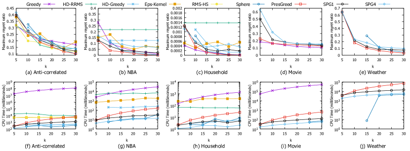
Figure 1: Performance comparisons. (a)-(e) show the maximum regret ratios of all the algorithms for different values of $k$, and (f)-(j) show the CPU times for different values of $k$.

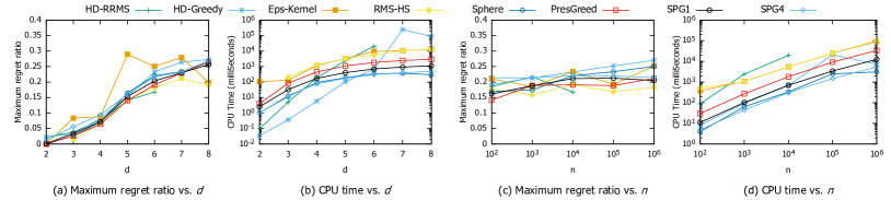
Figure 2: Performance comparisons. (a), (c) and (b), (d) show the maximum regret ratios and CPU times of all the algorithms for different values of $d$ and $n$ on the anti-correlated dataset respectively.

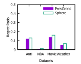
(a) No Sampling

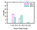
(b) Anti-correlated

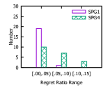
(c) NBA

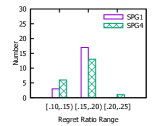
(d) Movie

(e) Weather

Figure 3: Distributions of regret ratios. (a) shows the regret ratios on 4 datasets of PresGreed without sampling, and (b)-(e) show the regret ratio distributions of 20 repeated experiments of the StocPresGreed algorithm at $k=25$ on these datasets.

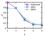
(a) Anti-correlated

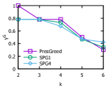
(b) NBA

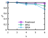
(c) Household

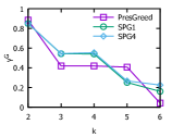
(d) Movie

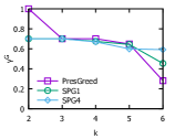
(e) Weather

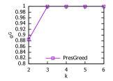
(f) Anti-correlated

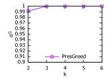
(g) NBA

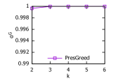
(h) Household

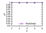
(i) Movie

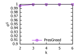
(j) Weather

Figure 4: Performance comparisons. (a)-(e), (f)-(j) show the submodularity ratios and curvatures respectively for different values of $k$ on Anti-correlated, NBA, Household, Movie and Weather.

IV-B Experiment Results

Maximum regret ratio and CPU time by varying $k$. In Figure 1, we report the maximum regret ratio and CPU time on all the datasets by varying $k$. We omit the result of the Greedy algorithm on the Weather dataset because it takes several days to obtain a solution. For the Eps-Kernel algorithm, the result size of this algorithm is much larger than $k$, so we randomly return $k$ points as the solution as in [6]. In high-dimensional datasets such as Movie and Weather, the HD-RRMS, HD-Greedy and Eps-Kernel algorithms all require too much memory to compute the solutions. Thus, we omit their performances in the Movie and Weather datasets. When $k<d$, HD-Greedy and Sphere do not work [13, 6], so we report their performance for $k\geq d$.

As shown, when $k$ is small, the maximum regret ratios of our proposed algorithms especially StocPresGreed are worse than the others. The reason is that StocPresGreed uses greedy policy and sampling to select points. But with $k$ increase, they are very close to each other except for the NBA and Household datasets. For the NBA dataset, our StocPresGreed performs better than HD-based algorithms and is comparable to others. In addition, when we need to select fewer data points in high-dimensional datasets (i.e., $k<d$), such as Movie and Weather, the Sphere algorithm does not work under this case, but our StocPresGreed algorithm can still perform well. PresGreed and StocPresGreed with different values of $\epsilon$ and $\lambda$ are very close to each other and decrease with $k$. For the real datasets, the maximum regret ratio is much smaller than that on the anti-correlated dataset, and they generally decrease with the values of $k$.

In terms of CPU time, by increasing $k$, the response time of all the algorithms increases since more data points are selected. Greedy, HD-RRMS and Eps-Kernel run much slower than the other algorithms on all the datasets. Under different settings of $\epsilon$ and $\lambda$, StocPresGreed constantly outperforms PresGreed and achieves up to 10 times speedup. The HD-Greedy algorithm is close to StocPresGreed, but it consumes a large amount of memory. Therefore, we omit it for the Movie and Weather datasets. The performance of StocPresGreed is close to Sphere and even better in the Household dataset. However, Sphere cannot work under the case of $k<d$. As can be observed, for different values of $\epsilon$ and $\lambda$, the maximum regret ratio reported by StocPresGreed is very close to that of PresGreed but with much better performance in CPU time.

In summary, we can observe that StocPresGreed provides very compelling performance and can make a tradeoff between the CPU time and the quality of returned results. Though our StocPresGreed algorithms sacrifices a little regret ratio, it can work under any circumstances, especially for the large high-dimensional datasets, e.g., the Weather dataset.

Maximum regret ratio and CPU time by varying $d$ and $n$. For large $d$ or $n$, Greedy and HD-RRMS are too time consuming. Therefore, we omit the evaluation of Greedy and some results of HD-RRMS here. In Figure 2(a)-(b), we conduct the experiments on the anti-correlated datasets by varying $d$. When $d$ increases, the maximum regret ratio and CPU time of all algorithms increase since more dimensions need to be processed. With the increase in $d$, the maximum regret ratios of different algorithms are very close to each other. However, the CPU times of PresGreed, Eps-Kernel and RMS-HS are always larger than that of StocPresGreed for different values of $\epsilon$ and $\lambda$. This is because PresGreed requires more function evaluations, Eps-Kernel needs more time to compute available coreset and RMS-HS consumes plenty of time to solve a large number of hitting-set problems. The CPU time of HD-RRMS increases very quickly and the performance drops quickly, especially in high-dimensional spaces. HD-Greedy performs better for $d<6$, but the query time is longer compared with StocPresGreed and Sphere when $d$ is large. This is because the discretized matrix in HD-Greedy can be large in high-dimensional spaces. The CPU time of StocPresGreed is close to Sphere, but Sphere has the aforementioned drawback when $k<d$. We vary $n$ on the anti-correlated dataset and the results are shown in Figure 2(c)-(d). Similar trends can be observed among the algorithms.

Regret ratio distribution. Since StocPresGreed is a sampling-based method, we report the regret ratio distribution here to demonstrate the stability of StocPresGreed under different $\epsilon$ and $\lambda$ settings. We run the algorithms 20 times with $k=25$ and record their distribution on all the datasets. The results are shown in Figure 3. Figure 3(a) only shows the regret ratios of the PresGreed and Sphere algorithms, which are the algorithms without sampling. The other nonsampling methods are quite time consuming, so we omit them. Figure 3(b)-(e) shows the regret ratio distribution for StocPresGreed. It records the number of times that the regret ratio has fallen into that interval. The size of each interval is set to approximately 0.05. We can see that most of the regret ratios of StocPresGreed are very close to those of PresGreed. The difference in the regret ratio between our StocPresGreed algorithm and the PresGreed algorithm does not exceed 0.1. For the anti-correlated and Movie datasets, the difference does not exceed 0.05. In addition, the difference of the regret ratio between our StocPresGreed algorithm and the Sphere algorithm is similar to that of PresGreed on the anti-correlated and NBA datasets. However, due to the high dimensions of the Movie and Weather datasets, Sphere either does not work or performs poorly when computing the $k$ results. Our StocPresGreed algorithm can still provide stable performance. We do not show the results on the Household dataset here, because the regret ratios of the PresGreed, StocPresGreed and Sphere algorithms are almost the same. Since the algorithms are conducted over the skyline points, the larger the skyline size is, the more effective our StocPresGreed algorithm will be.

Submodularity ratio and curvature. We compute the submodularity ratio for each $S_{i}$, where $i\in[1,k-1]$. The results are shown in Figure 4(a)-(e). We can see that the submodularity ratio is nonincreasing with the increase in $k$ for PresGreed. For the StocPresGreed algorithm, its submodularity ratio is not strictly nonincreasing with the increase in $k$, due to the randomness of StocPresGreed.

As illustrated in Figure 4(f)-(j), with the increase in $k$ the curvatures are almost equal to $1$ for PresGreed. According to the definition of curvature, for most cases, when $T\subseteq D$ and $|T|=k$, $\Delta_{S_{i-1}\cup T}(q_{i})=0$, which makes the curvature equal to 1. From Theorem 1, we can see that the approximation ratio approaches $1-1/e$. Thus, it verifies the advantages of the PresGreed algorithm.

The evaluation of $\epsilon$ and $\lambda$. In StocPresGreed, a larger $\epsilon$ or $\lambda$ denotes a smaller sample size. Here, we evaluate the performance of StocPresGreed by varying $\epsilon$ and $\lambda$ on the anti-correlated dataset. The results are shown in Figure 5(a)-(b). As we can observe, the maximum regret ratio does not change much when we vary $\epsilon$ or $\lambda$ over a wide range. However, the CPU time decreases considerably when the sample size drops.

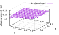
(a) Maximum regret ratio

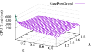
(b) CPU time

Figure 5: Performance comparisons. (a) and (b) show the maximum regret ratios and CPU times of the StocPresGreed for different values of $\epsilon$ and $\lambda$ on the anti-correlated datasets.

The upper bounds of maximum regret ratios. Since the RMS-HS, HD-Greedy and Eps-Kernel algorithms cannot output exact $k$ points, we report ony the upper bounds of the HD-RRMS and Sphere algorithms along with our proposed algorithms. As Figure 6(a)-(e) shows, the upper bound of the maximum regret ratio of HD-RRMS is smaller than others and closer to the maximum regret ratio of the optimal solution. However, HD-RRMS is time consuming as shown in Figure 1 and 2. The upper bounds of the maximum regret ratios of PresGreed and StocPresGreed are close to each other. For the Sphere algorithm, its upper bounds are decided by both $k$ and $d$. As shown in Figure 7, the upper bound of the maximum regret ratio increases with increasing $d$, but for $k$, it basically remains unchanged.

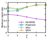
(a) Anti-correlated

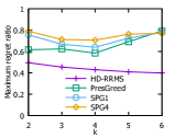
(b) NBA

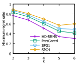
(c) Household

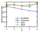
(d) Movie

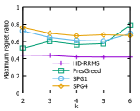
(e) Weather

Figure 6: Performance comparisons. (a)-(e) show the upper bounds of the maximum regret ratio for different values of $k$ on Anti-correlated, NBA, Household, Movie and Weather, respectively.

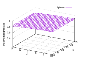
Figure 7: Upper bounds of the maximum regret ratio of Sphere for different values of $d$ and $k$.

V Related Work

Top-$k$ queries [1] and skyline queries [2] are two well-known tools for multi-criteria decision making that have received considerable attention during the last two decades. Improved versions are also investigated to improve the quality of the returned results, such as the subspace skyline [24], the constrained skyline [25, 26], the restricted skyline [27, 28], the $k$-dominant skyline query [29], top-$k$ representative skyline [30], distance-based representative skyline [31] and threshold-based preferences [32].

Due to the inherent limitations of top-$k$ and skyline queries, Nanongkai et al. [3] proposed the $k$-regret minimization problem. The problem is NP-hard, and a greedy strategy is proposed. However, the developed approach suffers from efficiency issues, and cannot scale well for large datasets. The following studies attempt to solve the problem from different perspectives. Peng et al. [4] attempted to reduce the candidate points from the whole skyline points to a small candidate set by using geometric properties. Cao et al. [11] and Agarwal et al. [12] proposed the $\epsilon$-kernel algorithm independently, which can keep the maximum regret ratio at most $\epsilon$ with an output size of $O(\epsilon^{-\frac{d-1}{2}})$. However, the output sizes of these algorithms are uncontrollable. They made output size from $O(\epsilon^{-\frac{d-1}{2}})$ to $k$. Then the upper bound was $O(k^{-\frac{2}{d-1}})$ [6]. Agarwal et al. [12] also proposed the hitting-set algorithm, which returns $O(k\log k)$ points. Asudeh et al. [13] interpreted the $k$-regret query in a $d$-dimensional dataset as a discretized matrix min-max problem and proposed two algorithms with upper bounds. Moreover, Xie et al. [6] designed the state-of-the-art Sphere algorithm whose upper bound on the maximum regret ratio was asymptotically optimal and restriction-free for datasets of any dimensionality. These bounds or theoretical results focus on the regret ratio instead of approximation guarantees. Qiu et al. [8] and Dong et al. [9] also provided the sampling techniques for 1-RMS and $k$-RMS queries, respectively. However, the proposed method in [8] is a special case of ours, where the sample factor equals 1, i.e., $\lambda=1$. Additionally, they both do not provide any approximation guarantees.

Several works extend Nanongkai et al. [3] to some extent. Chester et al. [33] introduced the relaxation to $k$-regret minimizing sets, denoted as the $k$-RMS query. The efficiency of the $k$-RMS query was further improved by [11] based on the $\epsilon$-kernel and [12, 34] via coresets and hitting sets. Faulkner et al. [5] and Qi et al. [7] extended the linear utility functions to Convex, Concave, CES utility functions and multiplicative utility functions for $k$-regret queries. Zeighami and Wong [35] proposed the metric of the average regret ratio to measure user satisfaction. To reduce the bounds of the regret ratio, Nanongkai et al. [23] and Xie et al. [36] combined user interactions into the process of selection. Additionally, based on regret minimization concepts, [13, 37, 38, 14] focus on compact maxima, rank regret representative problems, unified algorithms for different aggregate norms and min-size versions of the regret minimization query. To reduce the bounds of regret ratio, Nanongkai et al. [23] combine user’s interactions into the process of selection. Moreover, Xie et al. [36] provide a strongly truthful interactive mechanism to leverage the regret ratios using true database tuples instead of artificial ones and provide provable performance guarantees. Zeighami and Wong [39] propose the metric of average regret ratio to measure user’s satisfaction and further develop efficient algorithms to solve it [35]. Also, based on regret minimization concepts, [13, 37] focus on the compact maxima and rank regret representative problems, respectively. Moreover, the concept of the regret ratio is also adopted to solve the problems in the machine learning area, e.g., multi-objective submodular function maximization [40].

Due to the hardness of the problem, most of the studies utilize the greedy framework [4, 5, 6, 7, 8, 9]. However, there is still no strict theoretical analysis of the approximation ratio in the original greedy framework. We fill the theoretical gap, and our developed techniques can be used by the existing research if the greedy framework is used.

For summodularity aspect, submodular function maximization has numerous applications in machine learning and database systems [41, 42]. Though the problems are NP-hard, the greedy method can return a result with $1-1/e$ approximation ratio [17]. By leveraging the marginal gain property, lazy-update method is proposed to accelerate the search [43]. Badanidiyuru and Vondrák [44] propose a centralized algorithm that achieves a $(1-1/e-\epsilon)$ approximation ratio using $O(n/\epsilon\log(n/\epsilon))$ function evaluations for general submodular functions, and a multistage algorithm is proposed to further accelerate the search. In [21], a linear time algorithm is proposed for cardinality constrained submodular maximization, which provides the same approximation ratio as [44] with $n\log\frac{1}{\epsilon}$ function evaluations. The accelerated greedy algorithms [43, 21] start from an empty set, and need more time for picking the first data point. While the approaches in [44] require much more functions evaluations when $n$ is large, and they are more effective when those submodular functions can be easily decomposed and approximated. In a word, all the approaches in above are not efficient for large-scale datasets.

VI Conclusion

As an important operator, the $k$-regret minimization query is investigated to provide users with high-quality results from a large dataset. The existing solution is efficient, but there is still much space left for improvement, especially for larger datasets. In addition, the approximation ratio of the returned results of the greedy framework is not discussed in the literature. In this paper, we conduct the first theoretical analysis and provide an approximation guarantee for the previous RDPGreed greedy framework by utilizing the proposed happiness ratio concept. To reduce the evaluation cost and further speed up the processing, a sampling-based method, StocPresGreed, is proposed that provides an $(1-e^{-\frac{(1-\epsilon)(k-1)\gamma}{\lambda k}})$ approximation ratio. Moreover, careful analysis is presented to demonstrate the sample size required. Experiments over real-world and synthetic datasets were conducted to verify the advantages of the proposed methods.

References

- [1] I. F. Ilyas, G. Beskales, and M. A. Soliman, “A survey of top-k query processing techniques in relational database systems,” CSUR, vol. 40, no. 4, pp. 11:1–58, 2008.
- [2] S. Börzsöny, D. Kossmann, and K. Stocker, “The skyline operator,” in ICDE, 2001.
- [3] D. Nanongkai, A. D. Sarma, A. Lall, R. J. Lipton, and J. Xu, “Regret-minimizing representative databases,” in VLDB, 2010.
- [4] P. Peng and R. C.-W. Wong, “Geometry approach for k-regret query,” in ICDE, 2014.
- [5] T. K. Faulkner, W. Brackenbury, and A. Lall, “k-regret queries with nonlinear utilities,” in VLDB, 2015.
- [6] M. Xie, R. C.-W. Wong, J. Li, C. Long, and A. Lall, “Efficient k-regret query algorithm with restriction-free bound for any dimensionality,” in SIGMOD, 2018.
- [7] J. Qi, F. Zuo, H. Samet, and J. C. Yao, “K-regret queries using multiplicative utility functions,” TODS, vol. 43, no. 2, pp. 10:1–10:41, 2018.
- [8] X. Qiu, J. Zheng, Q. Dong, and X. Huang, “Speed-up algorithms for happiness-maximizing representative databases,” in APWeb-WAIM Workshops, 2018, pp. 321–335.
- [9] Q. Dong and J. Zheng, “Faster algorithms for k-regret minimizing sets via monotonicity and sampling,” in CIKM, 2019, pp. 2213–2216.
- [10] M. Xie, R. C.-W. Wong, and A. Lall, “An experimental survey of regret minimization query and variants: bridging the best worlds between top-k query and skyline query,” The VLDB Journal, vol. 29, pp. 147–175, 2020.
- [11] W. Cao, J. Li, H. Wang, K. Wang, R. Wang, R. C.-W. Wong, and W. Zhan, “k-regret minimizing set: Efficient algorithms and hardness,” in ICDT, 2017.
- [12] P. K. Agarwal, N. Kumar, S. Sintos, and S. Suri, “Efficient Algorithms for k-Regret Minimizing Sets,” in Proceedings of the 16th International Symposium on Experimental Algorithms (SEA), 2017.
- [13] A. Asudeh, A. Nazi, N. Zhang, and G. Das, “Efficient computation of regret-ratio minimizing set: A compact maxima representative,” in SIGMOD, 2017.
- [14] M. Xie, R. C. Wong, P. Peng, and V. J. Tsotras, “Being happy with the least: Achieving -happiness with minimum number of tuples,” in ICDE, 2020.
- [15] D. Bertsimas and J. Tsitsiklis, Introduction to Linear Optimization. Athena Scientific, 1997.
- [16] S. Fujishige, Submodular Functions and Optimization. Elsevier, 2005.
- [17] G. L. Nemhauser, L. A. Wolsey, and M. L. Fisher, “An analysis of approximations for maximizing submodular set functions—,” Mathematical Programming, vol. 14, no. 1, pp. 265–294, 1978.
- [18] A. Das and D. Kempe, “Submodular meets spectral: Greedy algorithms for subset selection, sparse approximation and dictionary selection,” in ICML, 2011.
- [19] A. A. Bian, J. M. Buhmann, A. Krause, and S. Tschiatschek, “Guarantees for greedy maximization of non-submodular functions with applications,” in ICML, 2017.
- [20] A. Krause and D. Golovin, “Submodular function maximization,” Tractability: Practical Approaches to Hard Problems, vol. 3, pp. 71–104, 2014.
- [21] B. Mirzasoleiman, A. Badanidiyuru, A. Karbasi, J. Vondrak, and A. Krause, “Lazier than lazy greedy,” in AAAI, 2015.
- [22] R. Khanna, E. Elenberg, A. Dimakis, S. Negahban, and J. Ghosh, “Scalable Greedy Feature Selection via Weak Submodularity,” in Proceedings of the 20th International Conference on Artificial Intelligence and Statistics (AISTATS), 2017.
- [23] D. Nanongkai, A. Lall, A. Das Sarma, and K. Makino, “Interactive regret minimization,” in SIGMOD, 2012.
- [24] Y. Yuan, X. Lin, Q. Liu, W. Wang, J. X. Yu, and Q. Zhang, “Efficient computation of the skyline cube,” in VLDB, 2005, p. 241–252.
- [25] D. Papadias, Y. Tao, G. Fu, and B. Seeger, “Progressive skyline computation in database systems,” TODS, vol. 30, no. 1, pp. 41–82, 2005.
- [26] M. Zhang and R. Alhajj, “Skyline queries with constraints: Integrating skyline and traditional query operators,” DKE, vol. 69, no. 1, pp. 153 – 168, 2010.
- [27] P. Ciaccia and D. Martinenghi, “Reconciling skyline and ranking queries,” in Proceedings of the VLDB Endowment, 2017, p. 1454–1465.
- [28] ——, “Flexible skylines: Dominance for arbitrary sets of monotone functions,” ACM Transactions on Database Systems (TODS), vol. 45, no. 4, 2020.
- [29] C. Y. Chan, H. V. Jagadish, K. Tan, A. K. H. Tung, and Z. Zhang, “Finding k-dominant skylines in high dimensional space,” in SIGMOD, 2006.
- [30] X. Lin, Y. Yuan, Q. Zhang, and Y. Zhang, “Selecting stars: The k most representative skyline operator,” in ICDE, 2007.
- [31] Y. Tao, L. Ding, X. Lin, and J. Pei, “Distance-based representative skyline,” in ICDE, 2009.
- [32] A. Das Sarma, A. Lall, D. Nanongkai, R. J. Lipton, and J. Xu, “Representative skylines using threshold-based preference distributions,” in ICDE, 2011.
- [33] S. Chester, A. Thomo, S. Venkatesh, and S. Whitesides, “Computing k-regret minimizing sets,” in VLDB, 2014.
- [34] N. Kumar and S. Sintos, “Faster approximation algorithm for the k-regret minimizing set and related problems,” in Proceedings of the 20th Workshop on Algorithm Engineering and Experiments (ALENEX), 2018.
- [35] S. Zeighami and R. C. Wong, “Finding average regret ratio minimizing set in database,” in ICDE, 2019.
- [36] M. Xie, R. C.-W. Wong, and A. Lall, “Strongly truthful interactive regret minimization,” in SIGMOD, 2019.
- [37] A. Asudeh, A. Nazi, N. Zhang, G. Das, and H. V. Jagadish, “RRR: rank-regret representative,” in SIGMOD, 2019.
- [38] S. Shetiya, A. Asudeh, S. Ahmed, and G. Das, “A unified optimization algorithm for solving regret-minimizing representative problems,” 2020.
- [39] S. Zeighami and R. C.-W. Wong, “Minimizing average regret ratio in database,” in SIGMOD, 2016.
- [40] T. Soma and Y. Yoshida, “Regret ratio minimization in multi-objective submodular function maximization,” in AAAI, 2017.
- [41] T. Soma, N. Kakimura, K. Inaba, and K.-i. Kawarabayashi, “Optimal budget allocation: Theoretical guarantee and efficient algorithm,” in ICML, 2014.
- [42] H. Lin and J. Bilmes, “A class of submodular functions for document summarization,” in Proceedings of the 10th Annual Conference of the North American Chapter of the Association for Computational Linguistics: Human Language Technologies (HLT-NAACL), 2011.
- [43] M. Minoux, “Accelerated greedy algorithms for maximizing submodular set functions,” in Proceedings of the 8th IFIP Conference on Optimization Techniques, 1978.
- [44] A. Badanidiyuru and J. Vondrák, “Fast algorithms for maximizing submodular functions,” in SODA, 2014.