Mass non-concentration at the nodal set and a sharp Wasserstein uncertainty principle

Abstract.

We prove $L^{p}$-mass concentration properties of Laplace eigenfunctions away from their nodal sets, extending a recent result in [GM3] to all dimensions, and giving a slight refinement of a result in [JN]. As a consequence, we are able to derive a sharp Wasserstein uncertainty principle that holds uniformly in the high frequency regime, proving a conjecture in [St1].

1. Introduction

Consider a closed $n$-dimensional Riemannian manifold $M$ with smooth metric $g$, and the Laplace-Beltrami operator $\Delta$ on $M$ (we use the analyst’s sign convention, namely, $-\Delta$ is positive semidefinite). It is known that in this setting $-\Delta$ has discrete spectrum $0=\lambda_{1}<\lambda_{2}\leq\dots\leq\lambda_{k}\nearrow\infty$, and an $L^{2}$-orthonormal basis of smooth eigenfunctions satisfying

$$-\Delta\varphi_{\lambda}=\lambda\varphi_{\lambda}.$$ (1)

We fix some definitions/notations. For an eigenvalue $\lambda$ of $-\Delta$ and a corresponding eigenfunction $\varphi_{\lambda}$, we denote the set of zeros (nodal set) of $\varphi_{\lambda}$ by $N_{\varphi_{\lambda}}:=\left\{x\in M:\varphi_{\lambda}(x)=0\right\}$. We call the connected components of $M\setminus N_{\varphi_{\lambda}}$ nodal domains. These are domains where the eigenfunction is not sign-changing (this follows from the maximum principle). As notation for a given nodal domain we use $\Omega_{\lambda}$, or just $\Omega$ with slight abuse of notation. Further, we denote the (metric) tubular neighbourhood of width $\delta$ around the nodal set $N_{\varphi_{\lambda}}$ by $T_{\delta}$. Generally, when two quantities $X$ and $Y$ satisfy $X\leq c_{1}Y$ and $X\geq c_{2}Y$, we write $X\lesssim Y$ and $X\gtrsim Y$ respectively. When both are satisfied, we write $X\sim Y$ in short. Normally, our estimates will be up to constants which might be dependent on the geometry of the manifold $(M,g)$, but definitely not on the eigenvalues $\lambda$. Throughout the paper, $|S|$ denotes the volume of a set $S$.

2. Mass concentration away from the nodal set

We are interested in investigating the mass (non)-concentration phenomenon on $T_{r}$, where $r\sim\lambda^{-1/2}$. In [GM3], the following result was proved:

Theorem 2.1 ([GM3]).

Let $M$ be a smooth closed Riemannian manifold with sectional curvature bound $K_{1}\leq\operatorname{Sec}_{M}\leq K_{2}$. There exists a positive constant $C_{1}$, depending only on $K_{i}$, such that for all small enough positive numbers $t,r$ (independent of $\lambda$) satisfying $0<t\leq r^{2}$, we have

$$\|\varphi_{\lambda}\|_{L^{1}(T_{r})}\geq\left(1-e^{-t\lambda}-C_{1}\Theta_{n}(r^{2}/t)\right)\|\varphi_{\lambda}\|_{L^{1}(M)},$$ (2)

where $\Theta_{n}(r^{2}/t)$ is the probability that a Euclidean Brownian particle starting at the origin exits $B(0,r)$ within time $t$.

Next, in dimension $n=2$, it was observed that one can use heat equation techniques in conjunction with harmonic measure theory (the latter not being available in higher dimensions) to obtain the reverse estimate:

Theorem 2.2 ([GM3]).

Let $M$ be a smooth closed Riemannian surface. Given a positive constant $C_{2}$, one can find positive constants $C_{3},\lambda_{0}$ such that for $\lambda\geq\lambda_{0}$, we have

$$\|\varphi_{\lambda}\|_{L^{p}\left(T_{r_{0}\lambda^{-1/2}}\right)}\leq C_{3}\left(1-e^{-pt_{0}}\right)^{1/p}\|\varphi_{\lambda}\|_{L^{p}(M)},\text{ for }p\in[1,\infty),$$ (3)

where $t_{0}\leq r_{0}^{2}\leq C_{2}$.

Our first goal in this paper is to extend Theorem 2.2 to all dimensions. To avoid inherent problems with the Brownian motion approach in higher dimensions, we completely forego working with heat theoretic apparatus as in [GM3], and revert back to ideas in elliptic pde. In particular, we mention the papers [JN, N, CM1] as motivating influences for our investigation here. We combine them with ideas and methods from [Ma, Ma1] that are well-known by now, and also some recent ideas in [L1, L2, LM]. We now state our first main result:

Theorem 2.3.

Let $M$ be a closed smooth Riemannian manifold. Then, for $p\in[1,\infty]$, there exists a positive constant $r_{p}(M,g)$ (independent of $\lambda$) such that if $\delta\lesssim r_{p}\lambda^{-1/2}$, we have that

$$\|\varphi_{\lambda}\|_{L^{p}\left(M\setminus T_{\delta}\right)}\gtrsim_{p,(M,g)}\|\varphi_{\lambda}\|_{L^{p}(M)}.$$ (4)

A few comments are in place.

• The nodal set of any eigenfunction $\varphi_{\lambda}$ is $C(M,g)\lambda^{-1/2}$-dense in $M$ for some $C(M,g)$ independent of $\lambda$. Clearly, in the regime $\delta\geq C(M,g)\lambda^{-1/2}$, we have that $T_{r}=M$. So in particular, the bound in (4) makes sense only in the regime $r<<C(M,g)\lambda^{-1/2}$.

• Theorems 2.1, 2.2 and 2.3 can be interpreted as shedding light on rough “aggregated” doubling/growth conditions. We recall that doubling indices of the type

  $$\log\frac{\sup_{B(x,2r)}|\varphi_{\lambda}|}{\sup_{B(x,r)}|\varphi_{\lambda}|},\quad x\in M,\quad r>0,$$ (5)

  have found extensive applications in the study of vanishing orders and nodal volumes (cf. [DF], [L1], [L2], [S]). A result of Donnelly-Fefferman ([DF]) states that such doubling indices are at most at the order of $\sqrt{\lambda}$. It is expected, however, that such a saturation happens rarely (cf. [DF], [L1]). In fact, on average the doubling indices should be bounded by a uniform constant (independent of $\lambda$) - we refer to the works of Nazarov-Polterovich-Sodin and Roy-Fortin ([NPS], [R-F]).

• As an illustrative example of Theorem 2.3, consider the case of the highest weight spherical harmonics $(x_{1}+ix_{2})^{l}$ on $S^{2}$ (as is well-known, the corresponding eigenvalue is $l(l+1)$). One can calculate that (up to constants)

  $${\|(x_{1}+ix_{2})^{l}\|_{L^{p}(S^{2})}^{p}=\frac{\Gamma\left(\frac{lp}{2}+1\right)}{\Gamma\left(\frac{lp}{2}+\frac{3}{2}\right)}\sim\left(\frac{lp}{2}+1\right)^{-\frac{1}{2}}}$$

  for high enough $l$ (see [Z1], Chapter 4). However, it follows from another standard computation that after converting to spherical coordinates, for high enough $l$, we have that

  $$\|\operatorname{Re}(x_{1}+ix_{2})^{l}\|_{L^{p}(T_{1/l})}^{p} \lesssim c_{2}(p)\int_{0}^{\frac{\pi}{2}}|\cos^{lp}\theta|\;d\theta\sim c_{2}(p)\frac{\Gamma\left(\frac{lp}{2}\right)}{\Gamma\left(\frac{lp}{2}+\frac{1}{2}\right)}\sim_{p}(lp)^{-1/2},$$

  where the constant $c_{2}(p)\searrow 0$ as $p\nearrow\infty$. This shows mass (non)concentration properties around nodal sets for Gaussian beams on $S^{2}$.

• The case $p=\infty$ in (4) being straightforward, we indicate the proof separately. Choose a point $x_{0}$ where $\varphi_{\lambda}$ achieves its maximum over $M$. Let us normalise $\|\varphi_{\lambda}\|_{L^{\infty}}=1$. Then, by standard elliptic estimates one can show that $\|\nabla\varphi_{\lambda}\|_{L^{\infty}}\leq C\sqrt{\lambda}$, which shows that there is a wavelength inscribed ball at $x_{0}$.

• The proof of Theorem 2.3 gives a slight refinement of Theorem 1 of [JN], see Remark 3.13 below.

2.1. Wasserstein distance and uncertainty principle

The concept of the Wasserstein metric as a “distance between two measures” was introduced in [V, D], and has now become mainstream in the study of optimal transport and allied applications to partial differential equations and geometry. The basic definitions and preliminaries required for our use have been outlined below in Section 4; for more details, we refer the reader to [Vi]. Of late, there has been a spurt of interest in uncertainty principles tied to the Wasserstein distance (see [St2, SS, CMO] and references therein). The typical such result is of the following form: given a “nice enough” function $f$ on a manifold $(M^{n},g)$, the product of the Wasserstein distance between the positive and negative parts of the function and the “size” of the zero set of the function (typically encoded by $(n-1)$-Hausdorff measure) is bounded below by some expression depending on $\|f\|_{L^{1}},\|f\|_{L^{\infty}}$, and the geometry $(M,g)$.

Here we wish to investigate this problem for the very special situation where $f$ is an eigenfunction of the Laplace-Beltrami operator. As a primary motivational example, consider the eigenfunctions $f_{k}:=\sin kx$ (or $\cos kx$) on the flat $2$-torus $\mathbb{T}^{2}=\mathbb{R}/(2\pi\mathbb{Z})\times\mathbb{R}/(2\pi\mathbb{Z})$. It is not trivial to explicitly evaluate the Wasserstein distance $W_{p}(f^{+}_{k},f^{-}_{k})$, but one can estimate that it has to be at the scale $\sim 1/k$. This is also quite intuitive, as $f^{\pm}_{k}$ are “off in phase” to the order of $\sim 1/k$, which is the scale as which mass transportation has to happen. But the problem becomes significantly harder when one considers linear combinations of $\sin kx$ and $\cos kx$, not to mention that such methods cannot even remotely approach the problem when one talks about spherical harmonics, and eigenfunctions on general Riemannian manifolds.

Now, consider a closed Riemannian manifold $(M,g)$ of dimension $n$ and let $\varphi_{\lambda}$ be a Laplace eigenfunction on $M$. Let $\varphi_{\lambda}^{+}:=\max\{\varphi_{\lambda},0\}$ and $\varphi_{\lambda}^{-}:=-\min\{\varphi_{\lambda},0\}$. We are interested in deriving general lower bounds on the Wasserstein distance $W_{1}(\mu,\nu)$, where $\mu=\varphi_{\lambda}^{+}\;dx$ and $\nu=\varphi_{\lambda}^{-}\;dx$, and $dx$ is the Riemannian volume element on $M$. Our proof uses properties which are rather specific to Laplace eigenfunctions, so we are able to prove a sharp bound with a rather simple expression, as conjectured in Section 3.3 of [St1] for the case $p=1$. With that in place, now we can state our second main result:

Theorem 2.4.

On a smooth closed Riemannian manifold $M$, we have that,

$$W_{1}(\varphi_{\lambda}^{+}\;dx,\varphi_{\lambda}^{-}\;dx)\gtrsim_{(M,g)}\frac{1}{\sqrt{\lambda}}\|\varphi_{\lambda}\|_{L^{1}(M)}.$$ (6)

Remark 2.5.

(a) The inequality (6) can be reversed in all dimensions, and has already been proved, see [St2, SS, CMO]. This completes the proof of the conjecture in [St1] for the case $p=1$. After the first version of this article was posted proving (6) in dimension $n=2$, (6) was proved in all dimensions and all $p\in[1,\infty)$ by [D-PF]. However, our original approach via heat equation, and our updated approach via doubling exponents and elliptic PDEs both seem quite different from the aforementioned paper.
(b) The example mentioned above for the torus $\mathbb{T}^{2}=\mathbb{R}/(2\pi\mathbb{Z})\times\mathbb{R}/(2\pi\mathbb{Z})$ shows that the estimate (6) is sharp in general.
(c) The comparability constant in (6) becomes a universal constant in the case of Euclidean domains.

Applying the estimate on the size of the nodal set in [Br], [L1], we have the following Wasserstein uncertainty principle (see Theorem 2 of [St2]) as an immediate consequence of Theorem 2.4:

Corollary 2.6 (Wasserstein uncertainty principle).

Let $M$ be a smooth closed Riemannian manifold, and let $\varphi_{\lambda}$ be normalised so that $|\varphi_{\lambda}|\;dx$ is a probability measure. Then, for high frequency $\lambda$, we have that

$$W_{1}(\varphi_{\lambda}^{+}\;dx,\varphi_{\lambda}^{-}\;dx)\;\mathcal{H}^{n-1}\left(N_{\varphi_{\lambda}}\right)\gtrsim_{(M,g)}1.$$ (7)

Here, $\mathcal{H}^{k}\left(N_{\varphi_{\lambda}}\right)$ represents the $k$-dimensional Hausdorff measure of the nodal set $N_{\varphi_{\lambda}}$. This falls in line with the heuristic described in [St2]: if $\mathcal{H}^{n-1}\left(N_{\varphi_{\lambda}}\right)$ is large, then one expects the nodal set $N_{\varphi_{\lambda}}$ to be highly dense, which implies that the positive and negative nodal domains are “close” to each other, which will lower the Wasserstein distance between them by making mass transportation more efficient. This heuristic makes sense in the opposite direction too. Also, note that one can just consider scalar multiples of $\varphi_{\lambda}$ without changing $N_{\varphi_{\lambda}}$, but the normalisation arising from the assumption of probability measure makes the uncertainty principle scale invariant.

3. Proof of Theorem 2.3

3.1. Preliminaries

3.1.1. Frequency functions and doubling exponents

First, we explain the following principle, following [DF], [N] and Section $2$ of [Ma1]: on a small scale comparable to the wavelength $1/\sqrt{\lambda}$, Laplace eigenfunctions behave qualitatively like harmonic functions. To see this, fix an atlas on $M$ for which all transition maps are bounded in $C^{1}$ norm, and let $g_{ij}$ denote the coefficients of the metric $g$ in local coordinates. In each chart, we have

$$\|g^{ij}\|_{C^{1}}\leq K_{1},g=\det g_{ij}\leq K_{2},$$ (8)

and the ellipticity bound

$$g^{ij}\xi_{i}\xi_{j}\geq K_{3}|\xi|^{2}.$$ (9)

In local coordinates, the eigenequation (1) reads:

$$-\frac{1}{\sqrt{g}}\partial_{i}(g^{ij}\sqrt{g}\partial_{j}\varphi_{\lambda})=\lambda\varphi_{\lambda}.$$ (10)

Since the above is satisfied pointwise, we can look in small balls $B_{r}=B(0,r)$, where $r=\frac{\sqrt{\varepsilon_{0}}}{\sqrt{\lambda}}$, and $\varepsilon_{0}$ is a small positive number to be chosen later (but independent of $\lambda$). Rescaling (10) to a unit ball $B_{1}$, we get

$$-\partial_{i}(g^{ij}_{r}\sqrt{g_{r}}\partial_{j}\varphi_{\lambda,r})=\varepsilon_{0}\sqrt{g_{r}}\varphi_{\lambda,r}\quad\text{on }B_{1},$$ (11)

where $\varphi_{\lambda,r}(x):=\varphi_{\lambda}(rx)$ is the scaled function obtained from $\varphi_{\lambda}$. Observe that we still have similar bounds as (8), (9) on the rescaled metric coefficients, as $r<1$.

If we let $a^{ij}=g_{r}^{ij}\sqrt{g_{r}},\text{ }q=\sqrt{g_{r}}$, we are in the following setting: let $B_{1}$ denote the unit ball in $\mathbb{R}^{n}$, and let $\varphi$ satisfy

$$L\varphi=0$$ (12)

on $B_{1}$, where $L$ is a second order elliptic operator with smooth coefficients. $L$ is of the form

$$Lu=L_{1}u-\varepsilon_{0}qu,$$ (13)

where

$$L_{1}u=-\partial_{i}(a^{ij}\partial_{j}u),$$

and we have the following properties:
(a) $a^{ij}$ is symmetric and satisfies the ellipticity bounds

$$\kappa_{1}|\xi|^{2}\leq a^{ij}\xi_{i}\xi_{j}\leq\kappa_{2}|\xi|^{2}.$$

(b) $a^{ij}$, $q$ are bounded by $\|a^{ij}\|_{C^{1}(\overline{B_{1}})}\leq K,\quad 0\leq q\leq K$. The main idea of the above principle is that, $\varepsilon_{0}$ can be chosen small enough so that $L$ is close to the Euclidean Laplacian (after a linear change of coordinates) and $\varphi$ displays behaviour similar to harmonic functions.

Next, we recall and collect a few relevant facts about doubling exponents and different notions of frequency functions - these include scaling and monotonicity results.

For $\varphi$ satisfying (12) in $B_{1}$, define for $r<1$ the following $r$-growth exponent:

$$\beta_{r}(\varphi)=\text{log }\frac{\sup_{B_{1}}|\varphi|}{\sup_{B_{r}}|\varphi|},$$ (14)

A fundamental result of  [DF] says the following:

Theorem 3.1.

There exist constants $C=C(M,g)>0$ and $r_{0}(M,g)>0$ such that for every point $p$ in $M$ and every $0<r<r_{0}$ the following growth exponent holds:

$$\sup_{B(p,r)}|\varphi_{\lambda}|\leq\left(\frac{r}{r^{\prime}}\right)^{C\sqrt{\lambda}}\sup_{B(p,r^{\prime})}|\varphi_{\lambda}|,\quad 0<r^{\prime}<r.$$ (15)

In particular, for a scaled eigenfunction $\varphi$ as defined above, we have

$$\frac{\beta_{r}(\varphi)}{\text{log}(1/r)}\lesssim\sqrt{\lambda}.$$ (16)

Closely related to the idea of doubling exponent is the concept of frequency function, which we now recall (see  [GL1],  [GL2]). For $u$ satisfying $L_{1}u=0$ in $B_{1}$, define for $a\in B_{1}$, $r\in(0,1]$ and $B(a,r)\subset B_{1}$,

$$D(a,r) =\int_{B(a,r)}|\nabla u|^{2}dV,$$

$$H(a,r) =\int_{\partial B(a,r)}u^{2}dS.$$

Then, define the generalized frequency of $\varphi$ by

$$\tilde{N}(a,r)=\frac{rD(a,r)}{H(a,r)}.$$ (17)

We note that  [L1] and  [L2] use a variant of $\tilde{N}(a,r)$, defined as follows:

$$N(a,r)=\frac{rH^{{}^{\prime}}(a,r)}{2H(a,r)}.$$ (18)

To pass between $\beta_{r}(\varphi),\tilde{N}(a,r)$ and $N(a,r)$, we record the following facts: from equation (3.1.22) of  [HL], we have that

$$H^{{}^{\prime}}(a,r)=\left(\frac{n-1}{r}+O(1)\right)H(a,r)+2D(a,r),$$ (19)

where $O(1)$ is a function of geodesic polar coordinates $(r,\theta)$ bounded in absolute value by a constant $C$ independent of $r$. More precisely, in [HL] a certain normalizing factor $\mu$ is introduced in the integrand in the definitions of $H(a,r)$ and $D(a,r)$. As it turns out by the construction, $C_{1}\leq\mu\leq C_{2}$ where $C_{1},C_{2}$ depend on the ellipticity constants of the PDE, the dimension $n$ and a bound on the coefficients (cf. 3.1.11, [HL]).

This gives us that when $\tilde{N}(a,r)$ is large, we have,

$$N(a,r)\sim\tilde{N}(a,r).$$ (20)

We also remark that the frequency $N(a,r)$ is almost-monotonic in the following sense: for any $\varepsilon>0$, there exists $R>0$ such that if $r_{1}<r_{2}<R$, then

$$N(a,r_{1})\leq N(a,r_{2})(1+\varepsilon).$$ (21)

This follows from (19) above and standard properties of $\tilde{N}(a,r)$ derived in [HL].

As regards growth exponents $\beta$, also of particular importance to us is the so-called doubling exponent of $\varphi_{\lambda}$ at a point, which corresponds to the case $r^{\prime}=\frac{1}{2}r$ in Theorem 3.1, and is defined as

$$\mathcal{N}(x,r)=\log\frac{\sup_{B(x,2r)}|\varphi_{\lambda}|}{\sup_{B(x,r)}|\varphi_{\lambda}|}.$$ (22)

One also naturally considers the $L^{p}$-variant of doubling exponents, namely,

Definition 3.2.

$$\mathcal{N}_{p}(x,r):=\log\frac{\|\varphi_{\lambda}\|^{p}_{L^{p}(B(x,2r))}}{{\|\varphi_{\lambda}\|^{p}_{L^{p}(B(x,r))}}}$$ (23)

We quickly state a lemma.

Lemma 3.3.

Up to constants depending on $p$, the doubling exponents in (22) and (23) are comparable, in the following precise sense:

$$\mathcal{N}\left(x,\frac{3}{4}r\right)\lesssim_{p}\mathcal{N}_{p}(x,r)\lesssim_{p}\mathcal{N}(x,r).$$ (24)

Proof.

Trivially, we have for any function $u$ that

$$\left(\int_{S}|u|^{p}\right)^{1/p}\leq\|u\|_{L^{\infty}(S)}\;|S|^{1/p}.$$

For the inequality in the other direction, it suffices if $u$ verifies $Lu\leq 0$, where $L$ is defined in (13). This follows from (29) below, and finishes the proof. ∎

Analogous to (21), there is also a monotonicity property for the doubling exponents $\mathcal{N}_{p}(x,r)$, see Lemma 2.2 of [LM] and references therein.

Now, consider an eigenfunction $\varphi_{\lambda}$ on $M$. We convert $\varphi_{\lambda}$ into a harmonic function in the following standard way. Let us consider the Riemannian product manifold $\bar{M}:=M\times\mathbb{R}$ - a cylinder over $M$, equipped with the standard product metric $\bar{g}$. By a direct check, the function

$$u(x,t):=e^{\sqrt{\lambda}t}\varphi_{\lambda}(x)$$ (25)

is harmonic. Note that till now, we have mentioned two seemingly unrelated classes of growth exponents, namely $\tilde{N}(a,r)$ for the harmonic function $u$ and $\mathcal{N}(x,r)$ for the eigenfunction $\varphi_{\lambda}$ (of course, the latter can also be defined equally easily for harmonic functions). We make the following

Convention 3.4.

$\mathcal{N}(x,r)$ will denote the doubling exponent of an eigenfunction in a ball $B(x,r)\subset M$, and $\tilde{N}(x,r)$ will denote the frequency function for the harmonic function $u(x,t)$ as in (25) in a ball $B((x,0),r)\subseteq M\times R_{0}\subset M\times\mathbb{R}$, where $R_{0}$ is a constant. When we say $\varphi_{\lambda}$ in controlled in the sense of frequency function on $B(x,r)\subseteq M$, we mean that $\tilde{N}(x,r)$ (or $N(x,r)$) is bounded by some constant independent of $\lambda$.

From the proof of Remark 3.1.4 of  [HL], one knows that they are related via the following:

$$\tilde{N}(x,r)\gtrsim\mathcal{N}(x,r^{\prime}),\quad r^{\prime}\in(0,\frac{r}{2}].$$ (26)

See also the related Theorem 3.1.3 of [HL].

Hence, by Theorem 3.1, the harmonic function $u$ in (25) has a doubling exponent which is also bounded by $C\sqrt{\lambda}$ in balls whose radius is no greater than $r_{1}=r_{1}(M,g)>0$.

It is well-known that doubling conditions imply upper bounds on the frequency (cf. Lemma $6$, [BL]):

Lemma 3.5.

For each point $p=(x,t)\in\bar{M}$ the harmonic function $u(p)$ satisfies the following frequency bound:

$$\tilde{N}(p,r)\leq C\sqrt{\lambda},$$ (27)

where $r$ is any number in the interval $(0,r_{2}),r_{2}=r_{2}(M,g)$ and $C>0$ is a fixed constant depending only on $M,g$.

For a proof of Lemma 3.5 we refer to Lemma $6$, [BL].

Finally, we need the following result, which is Lemma 7.4 of [L2]:

Lemma 3.6.

There exists $r=r(M,g)$ and $N_{0}=N_{0}(M,g)$ such that for any points $x_{1},x_{2}\in B(x,r)$ and $\tau$ such that $N(x_{i},\tau)>N_{0}$ and $\operatorname{dist}(x_{1},x_{2})<\tau<r$, there exists $C^{*}=C^{*}(M,g)>0$ such that

$$N(x_{2},C^{*}\tau)>\frac{99}{100}N(x_{1},\tau).$$

3.1.2. Local asymmetry of nodal domains

Our proof also uses the concept of local asymmetry of nodal domains, which roughly means the following. Consider a manifold $M$ with smooth metric. If the nodal set of an eigenfunction $\varphi_{\lambda}$ enters sufficiently deeply into a geodesic ball $B$, then the volume ratio between the positivity and negativity set of $\varphi_{\lambda}$ in $B$ is controlled in terms of $\lambda$. More formally, we have the following result from  [Ma1]:

$$\frac{|\{\varphi_{\lambda}>0\}\cap B|}{|B|}\gtrsim\frac{1}{\langle\beta_{1/2}(\varphi)\rangle^{n-1}},$$ (28)

where $\langle\beta_{r}\rangle=\text{max}\{\beta_{r},3\}$. In particular, when combined with the growth bound of Donnelly-Fefferman, this yields that

$$\frac{|\{\varphi_{\lambda}>0\}\cap B|}{|B|}\gtrsim\frac{1}{\lambda^{\frac{n-1}{2}}}.$$

This particular question about comparing the volumes of positivity and negativity seems to originate from [ChMu], [DF1], and then work of Nazarov, Polterovich and Sodin (cf. [NPS]), where they also conjecture that the present bound is far from being optimal. Moreover, the belief in the community seems to be that the sets of positivity and negativity should have volumes which are comparable up to a factor of $1/\lambda^{\epsilon}$ for small $\epsilon>0$.

3.1.3. Local elliptic maximum principle

We quote the following local maximum principle, which appears as Theorem 9.20 in  [GT].

Theorem 3.7.

Suppose $Lu\leq 0$ on $B_{1}$. Then

$$\sup_{B(y,r_{1})}u\leq C(r_{1}/r_{2},p)\left(\frac{1}{\operatorname{Vol}(B(y,r_{2}))}\int_{B(y,r_{2})}(u^{+}(x))^{p}dx\right)^{1/p},$$ (29)

for all $p>0$, whenever $0<r_{1}<r_{2}$ and $B(y,r_{2})\subseteq B_{1}$.

Notation 3.8.

By wavelength, we refer to the quantity $\lambda^{-1/2}$. When we say a ball $B(x,r)$ has wavelength radius, it means that the radius $r$ satisfies $r=c(M,g)\lambda^{-1/2}$. Also, for any ball $B:=B(x,r)$, let $\alpha B$ denote the ball $B(x,\alpha r)$, which is the concentric ball of radius $\alpha r$.

Before beginning the detailed proof of Theorem 2.3, we include a brief

Overall strategy and sketch of the proof.

We will take a covering of $M$ by wavelength balls, and show that at least a fixed percentage of the overall $L^{p}$-mass collects in balls of controlled growth exponent, also known as “good balls” (see Definitions 3.9 and 3.10 below). Since the nodal geometry is nicely behaved on good balls, one can further inscribe in each such good ball a (smaller) wavelength radius ball where $\varphi_{\lambda}$ is positive and another (smaller) wavelength radius ball where $\varphi_{\lambda}$ is negative. Then one justifies that either of these inscribed balls and their concentric half balls both collect at least a fixed fraction of the $L^{p}$-mass of the bigger good ball. The collection of these concentric half-balls will then be wavelength distance away from the nodal set, and still collect sufficient mass, proving (4).

∎

Now we start proving Theorem 2.3 formally.

Proof.

First, we start with a definition following the one in [CM1]. Now, we have

Definition 3.9.

A ball $B$ is called $d$-good in the sense of doubling exponent if we have that

$$\frac{\|\varphi_{\lambda}\|^{p}_{L^{p}(2B)}}{{\|\varphi_{\lambda}\|^{p}_{L^{p}(B)}}}\leq 2^{d}.$$ (30)

Naturally one has an analogue for the frequency function as well:

Definition 3.10.

A ball $B(x,r)\subseteq M$ is called $d$-good in the sense of frequency function if we have that

$$N\left(x,r\right)\leq d,$$ (31)

where $N(x,r)$ is calculated with respect to the harmonic function $u(x,t)$ in the ball $B((x,0),r)\subseteq M\times R_{0}$ (see Convention 3.4 above).

Now consider a covering of $M$ by balls $B_{j}$ of radius $r=\frac{r_{0}}{\sqrt{\lambda}}$ such that the nodal set enters deeply into each ball, that is, $N_{\varphi_{\lambda}}\cap\frac{1}{2}B_{j}\neq\emptyset$ for all $j$. We know that this is possible because of the wavelength density of the nodal set. We can also insist in addition on a controlled multiplicity of the covering, that is, each point $x\in M$ is contained in at most $C(M,g)$ of the balls $2B_{j}$ (this is possible from Bishop-Gromov volume comparison and the constant $C(M,g)$ depends only on the dimension and the lower bound on the Ricci curvature). Now we bring in the following idea from [CM1]: good balls (or, in other words, balls with controlled frequency function) in this collection will contain “most” of the mass of an eigenfunction $\varphi_{\lambda}$. Let $G_{d}$ denote the union of all the good balls in the above collection $\{B_{j}\}$ with controlled frequency function, in the sense of Convention 3.4. Because of the comparability estimates (20) and (26) and Lemma 3.3, we can say that such balls are “good” in the sense of Definition 3.9 also. Now, we prove the following

Lemma 3.11.

We have that

$$\|\varphi_{\lambda}\|_{L^{p}(G_{d})}\gtrsim_{C(M,g)}\|\varphi_{\lambda}\|_{L^{p}(M)}.$$ (32)

Proof.

Let $F_{d}$ denote the union of balls $B_{j}$ that are not $d$-good. Then, it suffices to estimate $\|\varphi_{\lambda}\|_{L^{p}(F_{d})}$ from above. We calculate that

$$\int_{F_{d}}|\varphi_{\lambda}|^{p}\leq\sum_{B_{j}\text{ not }d-\text{good}}\int_{B_{j}}|\varphi_{\lambda}|^{p}\leq 2^{-d}\int_{2B_{j}}|\varphi_{\lambda}|^{p}\leq C(M,g)2^{-d}\|\varphi_{\lambda}\|^{p}_{L^{p}(M)},$$

which gives the proof. ∎

Remark 3.12.

Observe that we have not really established (or claimed) how many “good balls” there are, merely the fact that most of the eigenfunction mass is concentrated on such balls. [CM1] establishes that there are at least (up to a geometric constant) $\lambda^{\frac{n+1}{4}}$ many good balls. This depends on a bound from [S], and it is not known whether this bound is optimal.

Now, consider a good ball $B_{i}$ from the covering considered above, and consider a smaller concentric ball $B_{i}^{\prime}:=r_{0}^{\prime}B_{i}$ of radius $r^{\prime}=\frac{r_{0}^{\prime}r_{0}}{\sqrt{\lambda}}$, where $r_{0}^{\prime}$ is a small enough constant that we will determine later. In case the nodal set still passes deeply through $B_{i}^{\prime}$, we can show (see for instance, the proof of Lemma 3.1 of [LM], which in turn seems to be motivated from Theorem 4.1 of [Ma1]) that we have a ball $\tilde{B}_{i}\subseteq B_{i}^{\prime}$ of radius $\frac{\tilde{r_{0}}r_{0}^{\prime}r_{0}}{\sqrt{\lambda}}$ such that $\varphi_{\lambda}|_{\tilde{B}_{i}^{\prime}}$ is positive (we remind the reader once again that all the above constants $r_{0},r_{0}^{\prime}$ and $\tilde{r_{0}}$ are independent of $\lambda$ and dependent only on the geometry $(M,g)$). Note that due to the almost-monotonicity of frequency function, $\varphi_{\lambda}$ has controlled doubling exponent on $B^{\prime}_{i}$. Now, choose a constant $\rho>1$ such that $B_{i}^{\prime}\subseteq\rho\tilde{B}_{i}\subseteq B_{i}$ (see diagram below). It is now clear that it suffices to choose $\rho$ such that the radius of $\rho\tilde{B_{i}}$ is equal to $2\frac{r^{\prime}_{0}r_{0}}{\sqrt{\lambda}}$, which is double the radius of $B^{\prime}_{i}$, and also equal to $\frac{r_{0}}{C^{*}\sqrt{\lambda}}$, where $C^{*}$ is the constant in Lemma 3.6 (observe that without loss of generality we can assume that $C^{*}\geq 2$). This gives that $r_{0}^{\prime}=\frac{1}{2C^{*}}$, which in turn determines $\tilde{r_{0}}$.

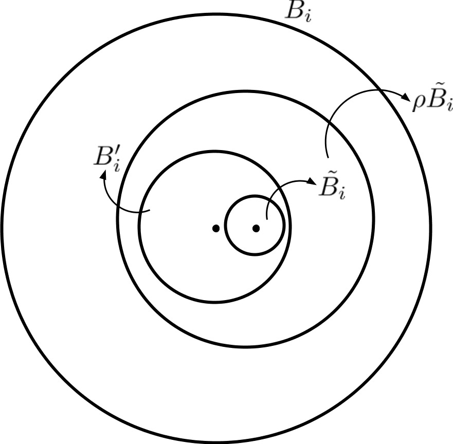
Figure 1. $B_{i}$, $B^{\prime}_{i}$, $\tilde{B}_{i}$ and $\rho\tilde{B}_{i}$

By monotonicity, we know that $B_{i}^{\prime}$ has controlled doubling exponent. This gives us that

$$\|\varphi_{\lambda}\|_{L^{p}(\rho\tilde{B}_{i})}\geq\|\varphi_{\lambda}\|_{L^{p}(B_{i}^{\prime})}\gtrsim\|\varphi_{\lambda}\|_{L^{p}(B_{i})}.$$

Also, by an application of Lemma 3.6, one sees that the frequency function and doubling exponent are controlled on $\rho\tilde{B_{i}}$. By almost monotonicity they are, in turn, also controlled on $\tilde{B}_{i}$. As a result,

$$\|\varphi_{\lambda}\|_{L^{p}(\tilde{B}_{i})}\gtrsim\|\varphi_{\lambda}\|_{L^{p}(\rho\tilde{B}_{i})}.$$

Finally, since the growth on $\tilde{B}_{i}$ is bounded, by monotonicity of the doubling exponent, we see that the growth on $\frac{1}{2}\tilde{B}_{i}$ is bounded, which means that

$$\|\varphi_{\lambda}\|_{L^{p}(\frac{1}{2}\tilde{B}_{i})}\gtrsim\|\varphi_{\lambda}\|_{L^{p}(\tilde{B}_{i})}.$$

At last, we have a collection $\tilde{\tilde{B}}_{j}:=\frac{1}{2}\tilde{B}_{j}$ such that

$$\|\varphi_{\lambda}\|_{L^{p}(H)}\gtrsim\|\varphi_{\lambda}\|_{L^{p}(M)},$$

where $H:=\cup_{j}\tilde{\tilde{B}}_{j}$, such that the nodal set is (up to a geometric constant) wavelength distance away from each of $\tilde{\tilde{B}}_{j}$.

∎

Remark 3.13.

Observe that the above proof gives us slightly more than claimed in the statement of Theorem 2.3, namely:

$$\|\varphi^{+}_{\lambda}\|_{L^{p}\left(M\setminus T_{\delta}\right)}\gtrsim_{p,(M,g)}\|\varphi_{\lambda}\|_{L^{p}(M)}\geq\|\varphi^{-}_{\lambda}\|_{L^{p}(M)}.$$

Replacing $\varphi_{\lambda}$ by $-\varphi_{\lambda}$, we can similarly conclude that

$$\|\varphi^{-}_{\lambda}\|_{L^{p}\left(M\setminus T_{\delta}\right)}\gtrsim_{p,(M,g)}\|\varphi_{\lambda}\|_{L^{p}(M)}\geq\|\varphi^{+}_{\lambda}\|_{L^{p}(M)}.$$

4. Wasserstein distance and proof of Theorem 2.4

4.1. Wasserstein metric

Given two measures $\mu,\nu$ on a metric space $M$, one defines the Wasserstein metric by

$$W_{p}(\mu,\nu)=\left(\inf_{\gamma\in\Gamma(\mu,\nu)}\int_{M\times M}d(x,y)^{p}\;d\gamma(x,y)\right)^{1/p},$$ (33)

where $\Gamma(\mu,\nu)$ denotes the set of all couplings of $\mu$ and $\nu$, that is, the collection of all measures on $M\times M$ with marginals $\mu$ and $\nu$.

The $1$-Wasserstein distance or Earth Mover’s Distance is the total amount of work (= distance $\times$ mass) required to move $\mu$ to $\nu$. Via the Monge-Kantorovich-Rubinstein duality one gets a particularly nice expression for the case $p=1$:

$$W_{1}(\mu,\nu)=\sup\left\{\int_{M}f\;d(\mu-\nu):f\text{ is }1-\text{Lipschitz }\right\}.$$ (34)

If one is primarily concerned with lower bounds, it is oftentimes more convenient to work with (34).

For a continuous function with mean zero, the Wasserstein distance between the measures corresponding to the positive and the negative parts of the function indicates how oscillatory the function is. If this is large enough, it should mean intuitively that the work done to move the positive mass to the negative mass should be large. This is antithetical to the function being too oscillatory, at least on the average.

4.2. Proof of (6)

We use the characterisation given in equation (34). This makes things easy as the Wasserstein distance is given as a supremum, and the whole problem boils down to the choice of a nice enough $1$-Lipschitz function $f$.

We begin by expressing $M$ as the disjoint union

$$M=\bigcup_{j=1}^{j_{0}}\Omega_{j}^{+}\cup\bigcup_{k=1}^{k_{0}}\Omega_{k}^{-}\cup N_{\varphi_{\lambda}},$$

where the $\Omega_{j}^{+}$ and $\Omega_{j}^{-}$ are the positive and negative nodal domains respectively of $\varphi_{\lambda}$. Then, we use $f\sim\frac{1}{\sqrt{\lambda}}$ on $\displaystyle{\bigcup_{j=1}^{j_{0}}\left(\Omega_{j}^{+}\setminus T_{r\lambda^{-1/2}}\right)}$, $f\sim-\frac{1}{\sqrt{\lambda}}$ on $\displaystyle{\bigcup_{k=1}^{k_{0}}\left(\Omega_{j}^{-}\setminus T_{r\lambda^{-1/2}}\right)}$, and the “linear interpolant” function in between. Such a function can be found in general as a variant of the following construction: consider a metric space $(X,d)$, and two open sets $Y,Z\subseteq X$. Assume that $d(Y,Z)=R$. Then one can find a $1$-Lipschitz function $f:X\to\mathbb{R}$ such that $f=\frac{R}{4}$ on $Y$, and $f=-\frac{R}{4}$ on $Z$, for example, the function $f(x)=\frac{R(d(x,Z)-d(x,Y))}{4(d(x,Z)+d(x,Y))}$. This immediately gives that

$$W_{1}(\varphi_{\lambda}^{+}\;dx,\varphi_{\lambda}^{-}\;dx)\gtrsim\frac{1}{\sqrt{\lambda}}\|\varphi\|_{L^{1}(M\setminus T_{r\lambda^{-1/2}})}.$$ (35)

With an appeal to Theorem 2.3 in the case $p=1$, we are done.

4.3. Acknowledgements

The author would like to thank Stefan Steinerberger, Emanuel Milman and Melchior Wirth for helpful conversations and correspondence. Special thanks are due to Alexander Logunov for suggesting some crucial ideas which allowed the author to prove Theorem 2.3 in dimensions $n\geq 3$. The author’s research was partially supported by SEED Grant RD/0519-IRCCSH0-024. Finally, the author wishes to thank Indian Institute of Technology Bombay for providing ideal working conditions.

References

- [A] L. Ahlfors, Conformal invariants: topics in geometric function theory, McGraw-Hill Book Co., New York, 1973, McGraw-Hill Series in Higher Mathematics.
- [B] C. Bär, On nodal sets for Dirac and Laplace operators, Comm. Math. Phys., 188 (1997), no. 3, 709 - 721.
- [BL] K. Bellová; and F. Lin, Nodal sets of Steklov eigenfunctions, Calc. Var. Partial Differential Equations, 54 (2015), no. 2, 2239 - 2268.
- [BHV] M. van den Berg, R. Hempel, and J. Voigt, -estimates for eigenfunctions of the Dirichlet Laplacian, J. Spectr. Theory 5 (2015), no. 4, 829 - 857.
- [Br] J. Brüning, Über Knoten von Eigenfunktionen des Laplace-Beltrami-Operators. (German), Math. Z., 158 (1978), no. 1, 15 - 21.
- [CMO] T. Carroll, X. Massaneda and J. Ortega-Cerdá, An enhanced uncertainty principle for the Vaserstein distance, arXiv:2003.03165v3.
- [ChMu] S. Chanillo and B. Muckenhoupt, Nodal geometry on Riemannian manifolds, J. Diff. Geom., 34 (1991), no. 1, 85- 91.
- [CM] T. Colding and W. Minicozzi II, Volumes for eigensections, Geom. Dedicata, 102 (2003), 19 - 24.
- [CM1] T. Colding and W. Minicozzi II, Lower bounds for nodal sets of eigenfunctions, Comm. Math. Phys. 306 (2011), no. 3, 777 - 784.
- [D-PF] N. De Ponti and S. Farinelli, Eigenfunctions and a lower bound on the Wasserstein distance, arXiv:2104.12097.
- [D] R. L. Dobrusin, Definition of a system of random variables by means of conditional distributions, (Russian. English summary) Teor. Verojatnost. i Primenen. 15 (1970), 469 - 497.
- [DF] H. Donnelly and C. Fefferman, Nodal sets of eigenfunctions on Riemannian manifolds, Invent. Math., 93 (1988), no. 1, 161 - 183.
- [DF1] H. Donnelly and C. Fefferman, Growth and geometry of eigenfunctions of the Laplacian, Analysis and partial differential equations, Lecture Notes in Pure and Appl. Math., vol. 122, Dekker, New York, 1990, pp. 635 - 655.
- [GL1] N. Garofalo and F. Lin, Monotonicity properties of variational integrals, weights and unique continuation, Indiana U. Math. J., 35 (1986), no. 2, 245 - 268.
- [GL2] N. Garofalo and F. Lin, Unique continuation for elliptic operators: a geometric-variational approach, Comm. Pure Appl. Math., 40 (1987), no. 3, 347 - 366.
- [GM1] B. Georgiev and M. Mukherjee, Nodal geometry, heat diffusion and Brownian motion, Anal. PDE, 11 (2018), no. 1, 133 - 148.
- [GM2] B. Georgiev and M. Mukherjee, On maximizing the fundamental frequency of the complement of an obstacle, C. R. Math. Acad. Sci. Paris, 356 (2018), no. 4, 406 - 411.
- [GM3] B. Georgiev and M. Mukherjee, Some applications of heat flow to Laplace eigenfunctions, preprint (arXiv:2109.00710).
- [GM4] B. Georgiev and M. Mukherjee, Some remarks on nodal geometry in the smooth setting. Calc. Var. Partial Differential Equations 58 (2019), no. 3, Paper No. 93, 25 pp.
- [GT] D. Gilbarg and N. Trudinger, Elliptic Partial Differential Equations of Second Order, Reprint of the 1998 edition. Classics in Mathematics. Springer-Verlag, Berlin (2001).
- [GS-C] A. Grigor’yan and L. Saloff-Coste, Hitting probabilities for Brownian motion on Riemannian manifolds, J. Math. Pures Appl. (9), 81 (2002), no. 2, 115 - 142.
- [HS] R. Hardt and L. Simon, Nodal sets for solutions of elliptic equations, J. Diff. Geom., 30 (1989), no. 2, 505 - 522.
- [HL] Q. Han and F. Lin, Nodal sets of solutions of elliptic differential equations, unpublished notes.
- [H] W. Hayman, Some bounds for principal frequency, Applicable Anal., 7 (1977/78), no. 3, 247 - 254.
- [JN] D. Jakobson and N. Nadirashvili, Quasi-symmetry of norms of eigenfunctions, Comm. Anal. Geom. 10 (2002), no. 2, 397 - 408.
- [JM] D. Jakobson and D. Mangoubi, Tubular neighborhoods of nodal sets and Diophantine approximation, Amer. J. Math., 131 (2009), no. 4, 1109 - 1135.
- [Ke] J. Kent, Eigenvalue expansions for diffusion hitting times, Z. Wahrsch. Verw. Gebiete, 52 (1980), no. 3, 309 - 319.
- [L] E. Lieb, On the lowest eigenvalue of the Laplacian for the intersection of two domains, Invent. Math., 74 (1983), no. 3, 441 - 448.
- [L1] A. Logunov, Nodal sets of Laplace eigenfunctions: proof of Nadirashvili’s conjecture and of the lower bound in Yau’s conjecture, Ann. of Math. (2), 187 (2018), no. 1, 241 - 262.
- [L2] A. Logunov, Nodal sets of Laplace eigenfunctions: polynomial upper estimates of the Hausdorff measure, Ann. of Math. (2), 187 (2018), no. 1, 221 - 239.
- [LM] A. Logunov and E. Malinnikova, Nodal sets of Laplace eigenfunctions: estimates of the Hausdorff measure in dimension two and three, 50 years with Hardy spaces, 333–344, Oper. Theory Adv. Appl., 261, Birkhäuser/Springer, Cham, 2018.
- [Ma] D. Mangoubi, On the inner radius of Nodal domains, Canad. Math. Bull. 51 (2008), no. 2, 249 - 260.
- [Ma1] D. Mangoubi, Local asymmetry and the inner radius of nodal domains. Comm. Partial Differential Equations 33 (2008), no. 7 - 9, 1611 - 1621.
- [MS] V. Maz’ya and M. Shubin, Can one see the fundamental frequence of a drum?, Lett. Math. Phys., 74 (2005), 135 - 151.
- [N] N. Nadirashvili, Metric properties of the eigenfunctions of the Laplace operator on manifolds, Ann. Inst. Fourier (Grenoble), 41 (1991), no. 1, 259 - 265.
- [NPS] F. Nazarov, L. Polterovich and M. Sodin, Sign and area in nodal geometry of Laplace eigenfunctions, Amer. J. Math., 127 (2005), no. 4, 879 - 910.
- [R-F] G. Roy-Fortin, Nodal sets and growth exponents of Laplace eigenfunctions on surfaces, Anal. PDE 8 (2015), no. 1, 223 - 255.
- [SS] A. Sagiv and S. Steinerberger, Transport and interface: an uncertainty principle for the Wasserstein distance, SIAM J. Math. Anal. 52 (2020), no. 3, 3039 - 3051.
- [S] C. Sogge, Concerning the norm of spectral clusters for second-order elliptic operators on compact manifolds, J. Funct. Anal. 77 (1988), no. 1, 123 - 138.
- [S1] C. Sogge, Problems related to the concentration of eigenfunctions, arXiv:1510.077223.
- [St] S. Steinerberger, Lower bounds on nodal sets of eigenfunctions via the heat flow, Comm. Partial Differential Equations, 39 (2014), no. 12, 2240 – 2261.
- [St1] S. Steinerberger, Wasserstein Distance, Fourier Series and Applications, Monatshefte Math., 194 (2021), 305 - 338.
- [St2] S. Steinerberger, A metric Sturm-Liouville theory in two dimensions, Calc. Var. Partial Differential Equations, 59 (2020), no. 1, Paper No. 12, 14 pp.
- [V1] S. Varadhan, Diffusion processes in a small time interval, Comm. Pure Appl. Math.. 20 (1967), 659 - 685.
- [V] L. N. Vasershtein, Markov processes over denumerable products of spaces describing large system of automata, Problems Inform. Transmission, 5 (1969), no. 3, 47 - 52.
- [Vi] C. Villani, Topics in Optimal Transportation, Graduate Studies in Mathematics, AMS, Providence (2003).
- [Z1] S. Zelditch, Eigenfunctions of the Laplacian on Riemannian Manifolds, Preprint available at https://sites.math.northwestern.edu/ zelditch/Eigenfunction.pdf.