Numerical simulation and entropy dissipative cure of the carbuncle instability for the shallow water circular hydraulic jump

Abstract

We investigate the numerical artifact known as a carbuncle, in the solution of the shallow water equations. We propose a new Riemann solver that is based on a local measure of the entropy residual and aims to avoid carbuncles while maintaining high accuracy. We propose a new challenging test problem for shallow water codes, consisting of a steady circular hydraulic jump that can be physically unstable. We show that numerical methods are prone to either suppress the instability completely or form carbuncles. We test existing cures for the carbuncle. In our experiments, only the proposed method is able to avoid unphysical carbuncles without suppressing the physical instability.

1 Introduction

1.1 Numerical shock instabilities

In [33] a numerical instability was observed to appear near the symmetry plane in the simulation of a bow shock. This phenomenon, subsequently dubbed “carbuncle", has been observed by many researchers in similar numerical experiments for the Euler equations, and many remedies have been proposed, mainly in the form of additional numerical dissipation [34, 32, 10, 5, 19, 37]. Most notably, dissipative Riemann solvers like HLLE and Rusanov suppress the carbuncle instability [34]. For a recent review of numerical shock instability and work to alleviate it, we refer to [38, Section 2.5].

Given the similarity of structure between the Euler equations and the shallow water equations, it is not surprising that carbuncles appear in numerical solutions of the latter as well [21]. The shallow water carbuncle behaves similarly to the Euler carbuncle; for instance, it appears when the Roe solver is used, but not when the HLLE or Rusanov solver is used, and can also be suppressed by particular modifications of the Roe solver [21, 2]. In this work, we propose a new Riemann solver that blends those of Rusanov and Roe based on a local measure of the entropy residual, as in [16, 15, 14]. Using this Riemann solver (within the second-order Lax-Wendroff-LeVeque finite volume scheme [27, 28]) supresses the formation of carbuncles while maintaining an accuracy similar to that of Roe solver.

The most common test problems used to investigate carbuncle formation are that of bow shock formation or a steady, grid-aligned planar shock. In both of these problems, the correct behavior is the formation of a stable shock profile without carbuncles. This is achieved by certain methods designed specifically to avoid carbuncles, but also by typical first-order accurate methods. Thus these test problems are not adequate on their own to evaluate methods for practical calculations. Elling [12] proposed instead a problem specifically designed to feature a carbuncle as the physical solution. This has been used as a test problem to identify methods that impose excessive dissipation.

Herein we introduce a new and more exacting test problem that arises in a common physical setting. Like some of the problems above, it includes an equilibrium solution consisting of a steady shock. Similar to the Elling problem, the equilibrium is unstable. However, the correct manifestation of the instability is different from the carbuncle. This allows us to distinguish schemes that yield correct behavior from both those that are too dissipative and those that generate carbuncles.

In the present work, we provide a test problem that possesses a genuine instability that leads to carbuncles in many numerical approximations. This is an ideal test for assessing numerical methods, since neither the presence of carbuncles nor the complete absence of instability represents the correct behavior. This test problem is the circular hydraulic jump.

1.2 The circular hydraulic jump

Perhaps the first reference to the observation of the circular hydraulic jump comes from Lord Rayleigh [36], who wrote that it “may usually be seen whenever a stream of water from a tap strikes a horizontal surface”. This phenomenon that is familiar in the everyday kitchen sink, is in fact highly nonlinear and unintuitive. Near the jet, the flow is shallow and supercritical, while further away it is deeper and subcritical. The transition from supercritical to subcritical flow occurs in a very narrow region and takes the form of a jump or bore that is roughly circular if the surface is flat; we refer to it herein as a circular hydraulic jump (CHJ).

Early experimental work on the CHJ began some time later [24, 42, 44]. Watson [44] derived the jump radius implied by Rayleigh’s approach and the vertical velocity profile in the supercritical region, assuming a no-slip boundary condition at the bottom. He also studied the turbulent flow case and performed experiments. More detailed experiments revealed different qualitative classification of jumps [17, 7]. Although later work incorporated more physical details (such as surface tension) into the models [4], Bohr et. al. showed that important properties of the jump (particularly its radius) could be reasonably predicted using a simple shallow water model [3].

While the jump is roughly circular, under appropriate conditions it may deviate from this shape and deform rapidly and chaotically in time. Instability of the jump was observed from fairly early on [7]. Under special circumstances with more viscous fluids, the jump instability may lead to the formation of curious shapes such as polygons [11], but for a low-viscosity fluid like water the behavior is generally chaotic. The strength of the instability increases with the jet velocity and with the depth at the outside of the jump. For fluids with finite viscosity, the flow can also be completely steady for sufficiently small velocities and depths.

As we will see, carbuncles can appear in the numerical solution of the shallow water circular hydraulic jump. This is natural, since the solution involves a standing shock wave. Dealing with the carbuncle in this context is particularly interesting and challenging, since this standing shock should (at least in an appropriate flow regime) be unstable, and some research has suggested that the carbuncle is the manifestation of a true physical instability [29, 12].

In this work, we describe and study the circular hydraulic jump as a new test problem for shallow water discretizations. We solve this test problem using a novel Riemann solver that supresses the formation of carbuncles without dissipating important features of the solution.

1.3 Outline

In Section 2, we review some existing numerical methods for the shallow water equations, focusing on certain Riemann solvers. In Section 3, we propose a new Riemann solver that blends those of Roe and Rusanov in order to avoid carbuncles without being excessively dissipative. In Section 4, we use Clawpack to compare the performance of the new Riemann solver to existing solvers on several standard shallow water test problems. In Section 5, we study the circular hydraulic jump using the newly proposed solver. We find that although some existing methods behave acceptably on previous test problems, they are not capable of providing accurate solutions for the circular hydraulic jump across the range of flow regimes we study. Some conclusions and future directions are discussed in Section 6.

2 Numerical methods for the shallow water equations

We consider the shallow water model in two horizontal dimensions:

$$h_{t}+(hu)_{x}+(hv)_{y} =0$$ (1a)

$$(hu)_{t}+\left(hu^{2}+\frac{1}{2}gh^{2}\right)_{x}+(huv)_{y} =0$$ (1b)

$$(hv)_{t}+(huv)_{x}+\left(hv^{2}+\frac{1}{2}gh^{2}\right)_{y} =0.$$ (1c)

Here $h,u,$ and $v$ are respectively the depth and the $x$- and $y$-components of velocity, which are functions of the two spatial coordinates $(x,y)$ as well as time $t$. The gravitational force is proportional to $g$. The system (1) can be written in vector form as

$$q_{t}+\nabla\cdot f(q) =0,$$ (2)

where $q=[h,hu,hv]^{T}$ and the flux function $f$ is defined in accordance with (1).

In this work we study the behavior of certain shock-capturing finite volume methods based on the use of Riemann solvers. For simplicity, we discuss these solvers in the context of a 1-dimensional problem and mesh. In the numerical experiments in §4 we use second-order Strang splitting [39] to extend the method to multiple dimensions.

2.1 Wave propagation methods

Let $Q_{i}$ represent the average value of the set of conserved quantities over cell $i$, which extends from $x_{i-1/2}$ to $x_{i+1/2}$. At each time step and at each interface $x_{i-1/2}$, we approximately solve the Riemann problem with initial states $(Q^{n}_{i-1},Q^{n}_{i})$. The approximate solution consists of a set of traveling discontinuities or waves ${\mathcal{W}}^{p}_{i-1/2}$ and corresponding speeds $s^{p}_{i-1/2}$. We use the wave propagation framework developed by LeVeque [27, 28] and employed in the Clawpack software [6, 23], which implements the Lax-Wendroff-LeVeque (LWL) scheme

$$Q_{i}^{n+1}=Q_{i}^{n}-\frac{\Delta t}{\Delta x}\left[{\mathcal{A}}^{+}\!\!{\Delta}Q_{i-1/2}+{\mathcal{A}}^{-}\!\!{\Delta}Q_{i+1/2}\right]-\frac{\Delta t}{\Delta x}\left[\tilde{F}_{i+1/2}-\tilde{F}_{i-1/2}\right],$$ (3)

Upon defining $z^{+}:=\frac{1}{2}(z+|z|)$ and $z^{-}:=\frac{1}{2}(z-|z|)$, the fluctuations are given by

$${\mathcal{A}}^{+}\!\!{\Delta}Q_{i-1/2}:=\sum_{p}\left(s_{i-1/2}^{p}\right)^{+}{\mathcal{W}}_{i-1/2}^{p},\qquad{\mathcal{A}}^{-}\!\!{\Delta}Q_{i+1/2}:=\sum_{p}\left(s_{i+1/2}^{p}\right)^{-}{\mathcal{W}}_{i+1/2}^{p},$$ (4)

and represent the effect (to first order accuracy) of waves coming from the solution of the Riemann problem at each of the neighboring interfaces. Meanwhile, $\tilde{F}_{i\pm 1/2}$ are correction fluxes that make the method second-order accurate:

$$\tilde{F}_{i\pm 1/2}=\frac{1}{2}\sum_{p}|s_{i\pm 1/2}^{p}|\left(1-\frac{\Delta t}{\Delta x}|s_{i\pm 1/2}^{p}|\right)\tilde{\mathcal{W}}_{i\pm 1/2}^{p}.$$ (5)

Here $\tilde{{\mathcal{W}}}_{i\pm 1/2}^{p}$ is a limited version of ${\mathcal{W}}_{i\pm 1/2}^{p}$, usually based on a total variation diminishing limiter function.

We note that, for the conservative Riemann solvers we use herein, the LWL scheme (3) can be written equivalently in flux-differencing form:

$$Q_{i}^{n+1}=Q_{i}^{n}-\frac{\Delta t}{\Delta x}\left[{F}_{i+1/2}-{F}_{i-1/2}\right]-\frac{\Delta t}{\Delta x}\left[\tilde{F}_{i+1/2}-\tilde{F}_{i-1/2}\right],$$ (6)

with appropriately chosen first order fluxes ${F}_{i+1/2}$ and correction fluxes $\tilde{F}_{i-1/2}$. We will sometimes work with the first-order method obtained by setting the correction fluxes to zero:

$$Q_{i}^{n+1}=Q_{i}^{n}-\frac{\Delta t}{\Delta x}\left[{\mathcal{A}}^{+}\!\!{\Delta}Q_{i-1/2}+{\mathcal{A}}^{-}\!\!{\Delta}Q_{i+1/2}\right]=Q_{i}^{n}-\frac{\Delta t}{\Delta x}\left[{F}_{i+1/2}-{F}_{i-1/2}\right].$$ (7)

Next we briefly review two commonly-used Riemann solvers: those of Rusanov and Roe. We refer to [22] and references therein for a detailed description of these two Riemann solvers in the context of the shallow water equations. Neither of these solvers deals with the carbuncle instability in a fully satisfactory way. Rusanov’s solver suppresses the carbuncle but (unless the mesh is highly refined) is known to also suppress related real instabilities, while Roe’s solver exhibits carbuncles. Later we will combine these two solvers in order to better deal with shock instability. Both of these solvers satisfy the conservation property

$${\mathcal{A}}^{-}\!\!{\Delta}Q_{i-1/2}+{\mathcal{A}}^{+}\!\!{\Delta}Q_{i-1/2}={f}({Q}_{i})-{f}({Q}_{i-1}).$$ (8)

2.2 Rusanov’s Riemann solver

Rusanov’s solver approximates the Riemann solution with a single wave traveling in each direction. Both waves are assumed to travel with speed $\lambda^{\max}_{i-1/2}$, which is an upper bound on the wave speeds appearing in the true solution of the Riemann problem. In this work, we take $\lambda_{i-1/2}^{\max}$ to be the upper bound from [1, Prop. 3.7]. The waves are then given by

$${\mathcal{W}}_{i-1/2}^{1,{\rm Rus}}={Q}_{i-1/2}-{Q}_{i-1},\qquad{\mathcal{W}}_{i-1/2}^{2,{\rm Rus}}={Q}_{i}-{Q}_{i-1/2},$$ (9)

where the intermediate state ${u}_{i-1/2}$ is determined by imposing conservation:

$$-\lambda_{i-1/2}^{\max}{\mathcal{W}}_{i-1/2}^{1,{\rm Rus}}+\lambda_{i-1/2}^{\max}{\mathcal{W}}_{i-1/2}^{2,{\rm Rus}}={f}({Q}_{i})-{f}({Q}_{i-1}).$$ (10)

The fluctuations are given by (4) with $s_{i-1/2}^{1}=-\lambda_{i-1/2}^{\max}$ and $s_{i-1/2}^{2}=\lambda_{i-1/2}^{\max}$, and the first- and second-order methods based on Rusanov’s solver are given by (7) and (3), respectively.

2.3 Roe’s Riemann solver

The Roe Riemann solver is based on evaluating the flux Jacobian using Roe’s average

$$\bar{h}_{i-1/2}=\frac{1}{2}(h_{i-1}+h_{i}),\qquad\hat{u}_{i-1/2}=\frac{\sqrt{h_{i-1}}u_{i-1}+\sqrt{h_{i}}u_{i}}{\sqrt{h_{i-1}}+\sqrt{h_{i}}},\qquad\hat{v}_{i-1/2}=\frac{\sqrt{h_{i-1}}v_{i-1}+\sqrt{h_{i}}v_{i}}{\sqrt{h_{i-1}}+\sqrt{h_{i}}}.$$ (11)

The waves and speeds are given by the eigenvectors and eigenvalues of the approximate flux Jacobian obtained using these averages, resulting in

$$\hat{\lambda}_{i-1/2}^{1}=\hat{u}_{i-1/2}-\sqrt{g\bar{h}_{i-1/2}},\qquad\hat{\lambda}_{i-1/2}^{2}=\hat{u}_{i-1/2},\qquad\hat{\lambda}_{i-1/2}^{3}=\hat{u}_{i-1/2}+\sqrt{g\bar{h}_{i-1/2}}.$$

and ${\mathcal{W}}_{i-1/2}^{p,{\rm Roe}}=\alpha_{i-1/2}^{p}\hat{r}_{i-1/2}^{p}$, with

$$\hat{r}^{1}_{i-1/2}=\begin{bmatrix}1\\ \hat{u}_{i-1/2}-\sqrt{g\bar{h}_{i-1/2}}\\ \hat{v}_{i-1/2}\end{bmatrix},\qquad\hat{r}^{2}_{i-1/2}=\begin{bmatrix}0\\ 0\\ 1\end{bmatrix},\qquad\hat{r}^{3}_{i-1/2}=\begin{bmatrix}1\\ \hat{u}_{i-1/2}+\sqrt{g\bar{h}_{i-1/2}}\\ \hat{v}_{i-1/2}\end{bmatrix}$$

and the factors $\alpha^{p}_{i-1/2}$ obtained by solving

$$\sum_{p}{\mathcal{W}}_{i-1/2}^{p,{\rm Roe}}=\left[\hat{r}^{1}_{i-1/2}~{}\hat{r}^{2}_{i-1/2}~{}\hat{r}^{3}_{i-1/2}\right]\begin{bmatrix}\alpha^{1}_{i-1/2}\\ \alpha^{2}_{i-1/2}\\ \alpha^{3}_{i-1/2}\end{bmatrix}=\Delta Q_{i-1/2}:={Q}_{i}-{Q}_{i-1}.$$ (12)

2.4 Kemm’s Riemann solver

Several specialized Riemann solvers have been proposed in order to deal with carbuncles. Among them, only that proposed by Kemm has been implemented and tested on the shallow water equations [21, 2]. The idea behind that solver, known as the HLLEMCC solver, is to combine the HLLE and Roe solvers in such a way that the resulting method behaves like Roe’s away from potential carbuncle instabilities, and like HLLE where the potential for such instabilities arises. This is done using an indicator function based on the local residual of the Rankine-Hugoniot condition for the shear wave. The method requires some parameters that may need to be tuned for a specific problem. We will consider this method in the numerical tests below.

3 An entropy-based blending of Rusanov and Roe

As we discussed in the introduction, finite volume methods that use a Roe Riemann solver are prone to exhibit the carbuncle instability. In contrast, methods that use Rusanov’s Riemann solver exhibit no carbuncles. However, such methods tend to dissipate other important physical features of the solution, unless the grid is highly refined. In this section we propose a Riemann solver that is carbuncle-free but avoids dissipating important features of the solution. To do so we first use a combination of Rusanov’s and Roe’s solvers, switching between them based on a local measure of the entropy residual. Previous works have also proposed blending Riemann solvers with different amounts of dissipation in the context of the Euler equations (see [30, 43, 20, 31, 9, 35]), the shallow water equations (see [2, 21]), and even the Navier-Stokes equations (see [30, 31]). Our approach differs from those just cited in that it is based on the local entropy; for a related approach in the context of the Euler equations, see [18, 19].

Since Roe’s solver is not entropy stable, the blended solver is also not guaranteed to be entropy stable. We therefore include an additional term that is chosen to give entropy stability, at least if the second-order correction fluxes are neglected. The complete proposed scheme can be written in flux-differencing form (6) using the first-order fluxes

$${F}_{i+1/2}=\frac{{f}({Q}_{i+1})+{f}({Q}_{i})}{2}-\frac{1}{2}\left(\theta_{i+1/2}\lambda_{i+1/2}^{\max}\mathbb{I}+(1-\theta_{i+1/2})|\hat{A}_{i+1/2}|+\lambda_{i+1/2}^{\min}\mathbb{I}\right)({Q}_{i+1}-{Q}_{i})$$ (13)

and correction fluxes (5) based on the Roe waves with modified speeds

$$s_{i+1/2}^{p}={\rm sgn}(\hat{\lambda}_{i+1/2}^{p})\lambda_{i+1/2}^{p}$$ (14)

where

$$\lambda_{i+1/2}^{p}:=\theta_{i+1/2}\lambda_{i+1/2}^{\max}+(1-\theta_{i+1/2})|\hat{\lambda}_{i+1/2}^{p}|+\lambda_{i+1/2}^{\min}.$$ (15)

Here $\mathbb{I}\in\mathbb{R}^{3\times 3}$ is the identity matrix, $\lambda_{i+1/2}^{\max}$ is the upper bound on the wave speed used in Rusanov’s Riemann solver (see §2.2), and $\hat{A}_{i+1/2}$ is Roe’s averaged flux Jacobian (see §2.3).

In the following sections we describe the properties of this solver and explain how $\theta_{i+1/2}$ and $\lambda^{\min}_{i+1/2}$ are chosen.

3.1 The entropy residual

Let $\eta^{\prime}(q)$ and $g(q)$ denote the entropy variable and entropy flux. Recall that $q=[h,hu,hv]^{T}$. We use the total energy as entropy; that is,

$$\eta(q)=\frac{1}{2}gh^{2}+\frac{(hu)^{2}+(hv)^{2}}{2h},\qquad g(q)=\frac{\eta(q)}{h}\begin{bmatrix}hu\\ hv\end{bmatrix}.$$

Based on [16], we consider

$$\int_{S_{i}}\eta^{\prime}(q)\cdot\left[\frac{\partial q}{\partial t}+\nabla\cdot{f}(q)\right]d{x}=\int_{S_{i}}\left[\frac{\partial\eta(q)}{\partial t}+\eta^{\prime}(q)\cdot\nabla\cdot{f}(q)\right]d{x}$$ (16)

as a measurement of the entropy production in cell $i$ (here $S_{i}=[x_{i-1/2},x_{i+1/2}]$). To avoid the need to compute the time derivative of the entropy, we follow [15, 14] and use $\int\frac{\partial\eta(q)}{\partial t}d{x}=-\int\nabla\cdot g(q)d{x}$, which holds in smooth regions. Then we define

$$\theta_{i}:=\frac{R_{i}}{D_{i}},$$ (17)

with

$$R_{i}=\left|\int_{S_{i}}\left[\eta^{\prime}(q)\cdot\nabla\cdot{f}(q)-\nabla\cdot g(q)\right]d{x}\right|,$$

and $D_{i}$ being an upper bound on $R_{i}$ so that $0\leq\theta_{i}\leq 1$. Note that $R_{i}\approx 0$ if $q$ is smooth in $S_{i}$. In our implementation, we use the approximation

$$R_{i} \approx\left|\eta^{\prime}({Q}_{i})\cdot\int_{S_{i}}\nabla\cdot{f}(q)d{x}-\int_{S_{i}}\nabla\cdot g(q)d{x}\right|=\left|\eta^{\prime}({Q}_{i})\cdot\int_{\partial S_{i}}{n}_{i}(s)\cdot{f}(q)d{s}-\int_{\partial S_{i}}{n}_{i}(s)\cdot g(q)d{s}\right|,$$ (18)

where ${n}_{i}$ denotes the unit vector normal to $\partial S_{i}$ pointing outward from cell $i$. To compute the boundary integrals, we approximate $q$ on each cell edge ${\mathcal{F}}_{ij}$ by the average of the two neighboring cell averages $\bar{Q}_{ij}=(Q_{i}+Q_{j})/2$, resulting in

$$R_{i}=\left|\sum_{{\mathcal{F}}_{ij}\in\partial S_{i}}|{\mathcal{F}}_{ij}|\left[\eta^{\prime}({Q}_{i})\cdot\left({n}_{ij}\cdot{f}\left(\bar{Q}_{ij}\right)\right)-{n}_{ij}\cdot g\left(\bar{Q}_{ij}\right)\right]\right|,$$ (19a)

where $$|{\mathcal{F}}_{ij}| {\mathcal{F}}_{ij} {n}_{ij} {\mathcal{F}}_{ij} i$$ is the length of and is the unit vector normal to pointing outward from cell . The normalization factor is similarly computed as

$$D_{i}=\sum_{k=1}^{d+1}\left|\eta^{\prime}_{k}\left({Q}_{i}\right)\right|\left|\sum_{{\mathcal{F}}_{ij}\in\partial S_{i}}|{\mathcal{F}}_{ij}|\left({n}_{ij}\cdot{f}\left(\bar{Q}_{ij}\right)\right)_{k}\right|+\left|\sum_{{\mathcal{F}}_{i}\in\partial S_{i}}|{\mathcal{F}}_{ij}|{n}_{ij}\cdot g\left(\bar{Q}_{ij}\right)\right|,$$ (19b)

where $(z)_{k}$ denotes the $k$-th component of $z\in\mathbb{R}^{d+1}$, and $d$ is the number of physical dimensions. In (13) we need values of $\theta$ at the cell interfaces, for which we use

$$\theta_{i+1/2}=\max(\theta_{i},\theta_{i+1}).$$

We expect that $\theta_{i+1/2}\approx 0$ in smooth regions, while $\theta_{i+1/2}\approx 1$ near shocks. The value of $\theta_{i+1/2}$ controls whether the first-order flux (13) behaves more like that of Rusanov or Roe. Specifically, if $\lambda_{i+1/2}^{\min}=0$ and $\theta_{i+1/2}=1$, the flux is equivalent to that of Rusanov, while if $\lambda_{i+1/2}^{\min}=0$ and $\theta_{i+1/2}=0$, it is equivalent to that of Roe.

In fact, with the choice (14), the correction fluxes also match those of Rusanov or Roe in the appropriate limit, as shown in the next section.

3.2 The correction fluxes

In this section we explain the choice of wave speeds (14). For the moment, we consider (13)-(15) without entropy stabilization; i.e., we set $\lambda^{\min}_{i+1/2}=0$ for now. We use ${\mathcal{W}}^{p,{\rm Rus}}$ to denote the waves in the Rusanov solver and ${\mathcal{W}}^{p,{\rm Roe}}$ to denote the waves in the Roe solver. The first-order method given by (7) with the numerical flux (13) can also be written in terms of fluctuations:

$${\mathcal{A}}^{+}\!\!{\Delta}Q_{i-1/2} =\frac{1}{2}\sum_{p}\left(\hat{\lambda}_{i-1/2}^{p}+\lambda_{i-1/2}^{p}\right){\mathcal{W}}_{i-1/2}^{p,{\rm Roe}},$$ (20a)

$${\mathcal{A}}^{-}\!\!{\Delta}Q_{i+1/2} =\frac{1}{2}\sum_{p}\left(\hat{\lambda}_{i+1/2}^{p}-\lambda_{i+1/2}^{p}\right){\mathcal{W}}_{i+1/2}^{p,{\rm Roe}}.$$ (20b)

To implement the correction fluxes required for the second-order scheme (3), we must also define a set of waves and corresponding speeds. Using only the waves from the Roe solver, it is in general not possible to choose speeds that yield the fluctuations (20), and we instead use (14). Using this in (5) and (20) in (3), we obtain (in the absence of limiting) the second-order scheme

$${Q}_{i}^{n+1}={Q}_{i}^{n} -\frac{\Delta t}{2\Delta x}\sum_{p}\left[\left(\hat{\lambda}_{i+1/2}^{p}-\frac{\Delta t}{\Delta x}(\lambda_{i+1/2}^{p})^{2}\right){\mathcal{W}}_{i+1/2}^{p,{\rm Roe}}+\left(\hat{\lambda}_{i-1/2}^{p}+\frac{\Delta t}{\Delta x}(\lambda_{i-1/2}^{p})^{2}\right){\mathcal{W}}_{i-1/2}^{p,{\rm Roe}}\right],$$ (21)

It is clear again that if $\theta_{i\pm 1/2}=0$ we recover the standard second-order Lax-Wendroff method based on Roe’s Riemann solver. We now show that if $\theta_{i\pm 1/2}=1$, we recover the Lax-Wendroff method based on Rusanov’s Riemann solver.

To see this, first consider (10) and rewrite the right-going fluctuation as follows:

$${\mathcal{A}}^{+,{\rm Rus}}\Delta Q_{i-1/2}:=\lambda_{i-1/2}^{\max}{\mathcal{W}}_{i-1/2}^{2,{\rm Rus}}={f}({Q}_{i})-{f}({Q}_{i-1})+\lambda_{i-1/2}^{\max}\left({\mathcal{W}}_{i-1/2}^{1,{\rm Rus}}+{\mathcal{W}}_{i-1/2}^{2,{\rm Rus}}\right)-\lambda_{i-1/2}^{\max}{\mathcal{W}}_{i-1/2}^{2,{\rm Rus}}.$$ (22)

From (9) and (12) we get ${\mathcal{W}}^{1,{\rm Rus}}_{i-1/2}+{\mathcal{W}}^{2,{\rm Rus}}_{i-1/2}={Q}_{i}-{Q}_{i-1}=\sum_{p}{\mathcal{W}}_{i-1/2}^{p,{\rm Roe}}$. Using (8) and (20), (22) becomes

$$\lambda_{i-1/2}^{\max}{\mathcal{W}}_{i-1/2}^{2,{\rm Rus}}=\sum_{p}\left(\hat{\lambda}_{i-1/2}^{p}+\lambda_{i-1/2}^{\max}\right){\mathcal{W}}_{i-1/2}^{p,{\rm Roe}}-\lambda_{i-1/2}^{\max}{\mathcal{W}}_{i-1/2}^{2,{\rm Rus}},$$

which implies that

$${\mathcal{A}}^{+,{\rm Rus}}\Delta Q_{i-1/2}=\frac{1}{2}\sum_{p}\left(\hat{\lambda}_{i-1/2}^{p}+\lambda_{i-1/2}^{\max}\right){\mathcal{W}}_{i-1/2}^{p,{\rm Roe}},$$ (23a)

and similarly,

$${\mathcal{A}}^{-,{\rm Rus}}\Delta Q_{i+1/2}=\frac{1}{2}\sum_{p}\left(\hat{\lambda}_{i+1/2}^{p}-\lambda_{i+1/2}^{\max}\right){\mathcal{W}}_{i+1/2}^{p,{\rm Roe}}.$$ (23b)

To get the second-order Lax-Wendroff method based on Rusanov’s Riemann solver, plug the fluctuations (23) into (3) where $\tilde{F}_{i\pm 1/2}$ is given by (5) with $|s^{p}_{i\pm 1/2}|=\lambda_{i\pm 1/2}^{\max}$ and $\tilde{\mathcal{W}}^{p}_{i\pm 1/2}={\mathcal{W}}_{i\pm 1/2}^{p,{\rm Roe}}$. By doing this, we get (21) (since $\theta_{i\pm 1/2}=1\implies\lambda_{i\pm 1/2}^{p}=\lambda_{i\pm 1/2}^{\max}$).

3.3 Entropy stabilization

In the previous section we neglected the term $\lambda^{\min}_{i+1/2}$ in (13). In this section, we follow [25] and show how this term is computed, in order to guarantee local entropy stability of the scheme given by using (13) in (7).

Let $\eta^{\prime}_{i}=\eta^{\prime}({Q}_{i})$ and $g_{i}=g({Q}_{i})$ denote the entropy variable and the (one-dimensional) entropy flux at cell $i$, respectively. Also let $\psi=\eta^{\prime}({Q}_{i})\cdot{f}({Q}_{i})-g({Q}_{i})$ be the entropy potential at cell $i$. From [40, §4], if the numerical fluxes satisfy

$$(\eta^{\prime}_{i}-\eta^{\prime}_{i-1})\cdot{F}_{i-1/2}\leq\psi_{i}-\psi_{i-1},\qquad(\eta^{\prime}_{i+1}-\eta^{\prime}_{i})\cdot{F}_{i+1/2}\leq\psi_{i+1}-\psi_{i},$$ (24)

then we have the entropy inequality

$$\frac{d\eta({Q}_{i})}{dt}+\frac{1}{\Delta x}\left[G_{i+1/2}-G_{i-1/2}\right]\leq 0,$$ (25)

where

$$G_{i+1/2} =\frac{1}{2}\left(\eta^{\prime}_{i}+\eta^{\prime}_{i+1}\right){F}_{i+1/2}-\frac{1}{2}(\psi_{i}+\psi_{i+1}),$$

is a discretization of the entropy flux. If (25) holds with equality, the scheme is entropy-conservative [41].

The approach in [41], is based on first developing an entropy-conservative scheme and then adding entropy dissipation to enforce (25). On the other hand, herein we have added dissipation (as described in Section 3.1) that does not guarantee (25). Indeed, some linear stabilization techniques that add artificial dissipation of the conserved variables are known to produce entropy; see for example [13, 26]. To guarantee (25), we add extra dissipation of the conserved variables via (26). Doing this counteracts entropy production created by any component of the Riemann solver; see for example [26] (in the context of $C^{0}$ finite elements).

Plugging (13) into the condition (24) yields the required value

$$\lambda_{i+1/2}^{\min}=\max\left\{0,\frac{\frac{1}{2}(\eta^{\prime}_{i+1}-\eta^{\prime}_{i})\cdot\left[{f}({Q}_{i+1})+{f}({Q}_{i})-\sum_{p}\lambda_{i+1/2}^{p,{\rm EV}}{\mathcal{W}}_{i+1/2}^{p,{\rm Roe}}\right]-(\psi_{i+1}-\psi_{i})}{\frac{1}{2}(\eta^{\prime}_{i+1}-\eta^{\prime}_{i})\cdot\sum_{p}{\mathcal{W}}_{i+1/2}^{p,{\rm Roe}}}\right\},$$ (26)

where

$$\lambda_{i+1/2}^{p,{\rm EV}}=\theta_{i+1/2}\lambda_{i+1/2}^{\max}+(1-\theta_{i+1/2})|\hat{\lambda}_{i+1/2}^{p}|.$$

With this choice, (13) guarantees (24), and therefore (25). Note that here we have used the identities

$$|\hat{A}_{i+1/2}|(Q_{i+1}-Q_{i})=\sum_{p}|\hat{\lambda}^{p}_{i+1/2}|{\mathcal{W}}^{p,{\rm Roe}}_{i+1/2},\qquad Q_{i+1}-Q_{i} =\sum_{p}{\mathcal{W}}^{p,{\rm Roe}}_{i+1/2}.$$

Since the blended Riemann solver described in Section 3 already tends to introduce entropy dissipation, we expect condition (24) to be fulfilled most of the time even with $\lambda_{i+1/2}^{\min}=0$. But (26) is used as a safeguard to guarantee entropy stability of the first-order method. Extra modifications would be needed to guarantee entropy stability of the second-order LWL method (3) and its multidimensional extension via Strang splitting. We do not pursue such modifications in this work.

We close this section with two remarks. First, note that the entropy stability condition (24) can be written equivalently in terms of fluctuations:

$$(\eta^{\prime}_{i}-\eta^{\prime}_{i-1})\cdot\Big{(}\underbrace{{f}({Q}_{i})-{\mathcal{A}}^{+}\Delta Q_{i-1/2}}_{={F}_{i-1/2}}\Big{)}\leq\psi_{i}-\psi_{i-1},\quad(\eta^{\prime}_{i+1}-\eta^{\prime}_{i})\cdot\Big{(}\underbrace{{f}({Q}_{i})+{\mathcal{A}}^{-}\Delta Q_{i+1/2}}_{={F}_{i+1/2}}\Big{)}\leq\psi_{i+1}-\psi_{i}.$$

Second, the additional dissipation introduced by $\lambda_{i\pm 1/2}^{\min}$ can also serve independently as an entropy fix for Roe’s solver, as we demonstrate via a numerical experiment in §4.1.

4 Numerical results

In this section we present one- and two-dimensional numerical experiments to demonstrate the behavior of the blended Riemann solver from §3 with the extra entropy dissipation from §3.3. We compare the behavior of the blended solver against the standard Roe’s and Rusanov’s solvers. In most of the experiments we use these Riemann solvers with the LWL method reviewed in §2.1. When the exact solution is available, we report convergence results based on the $L^{1}$-error for the water height

$$E_{1}=\sum_{i}|K_{i}|~{}|h_{i}-h^{e}({x}_{i})|,$$

where $|K_{i}|$ is the length or area of cell $i$, $h_{i}$ is the cell average of the water height at cell $i$, and $h^{e}({x}_{i})$ is the exact water height evaluated at the center of cell $i$. Since the methods under consideration are at most second order accurate, comparison of cell averages with centered point values is a sufficient way to test their accuracy. In all experiments we use $g=1$.

We consider a total of five problems. We start in §4.1 with a one-dimensional Riemann problem over a dry bed. For this problem we use the first-order methods (7), to avoid negative depth values. Although only Rusanov’s solver is proven to guarantee positivity, we do not get negative values for the water height with any of the first-order methods. In §4.2 we apply the second-order methods to a dam-break problem with a wet bed. This problem contains strong shocks. We observe similar accuracy with the blended solver or the Roe solver; this suggests that the extra numerical entropy dissipation that the blended solver introduces near the shocks does not degrade the accuracy of the underlying Roe solver. This extra dissipation, however, prevents the formation of carbuncles in other experiments, which we demonstrate in §4.3 and §5.4. In §5.2 we consider a one-dimensional problem with a smooth steady state solution. We observe the expected second-order accuracy of method (3) with Roe’s and the blended solvers. Using Rusanov’s Riemann solver degrades the accuracy to first-order. The overall accuracy of the blended solver is not degraded since the extra dissipation is not applied in smooth regions. The main focus of this work is in the formation of carbuncle instabilities in the two-dimensional CHJ. We present an extensive set of experiments for this problem in §5.4. We consider not only Roe’s, Rusanov’s and the blended solvers, but also the solver proposed in [21], which is designed to remove the carbuncle instabilities in the shallow water equations.

4.1 Dam break problem on a dry bed

We start with the one-dimensional dam break problem on a dry bed. This problem is a canonical example that demonstrates the ‘entropy glitch’ of Roe’s solver at transonic rarefactions. Since the baseline Roe solver we use (see §2.3) does not contain an entropy fix, it is important to demonstrate that the blended Riemann solver fixes the entropy glitch. We follow the setup in [8, §4.1.2]. The domain is given by $x\in(0,10)$, and the initial condition is $hu(x,0)=0$ and

$$h(x,0)=\begin{cases}h_{l}&x\leq x_{0}=5\\ h_{r}&x>x_{0},\end{cases}$$

with $h_{l}=5\times 10^{-3}$. In our experiments we use $h_{r}=1\times 10^{-15}$ to avoid division by zero. The exact solution, which can also be found in [8] and references therein, is

$$h(x,t)=\begin{cases}h_{l},\\ \frac{4}{9g}\left(\sqrt{gh_{l}}-\frac{x-x_{0}}{2t}\right)^{2},\\ 0,\end{cases}\quad u(x,t)=\begin{cases}0,&\mbox{ if }x\leq x_{A}(t),\\ \frac{2}{3}\left(\sqrt{gh_{l}}+\frac{x-x_{0}}{t}\right),&\mbox{ if }x_{A}(t)<x\leq x_{B}(t),\\ 0,&\mbox{ if }x_{B}(t)<x,\end{cases}$$

with $x_{A}(t)=x_{0}-t\sqrt{gh_{l}}$ and $x_{B}=x_{0}+2t\sqrt{gh_{l}}$. We solve the problem up to $t=10$. In Figures 1a-1c, we show the solution using method (7) with Roe’s solver, Rusanov’s solver and the blended solver, respectively. The entropy glitch, which is manifested as a non-physical shock at $x=x_{0}$, is present with Roe’s solver. Using Rusanov’s and the blended solvers fixes the entropy glitch. In Table 1, we summarize the results of a convergence test. Note that using the blended solver leads to more accurate results.

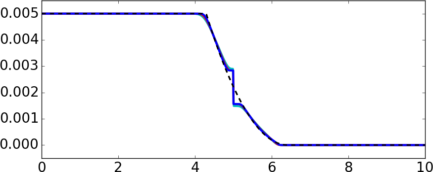
(a) Roe’s Riemann solver.

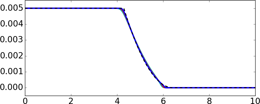
(b) Rusanov’s Riemann solver.

(c) Blended Riemann solver.

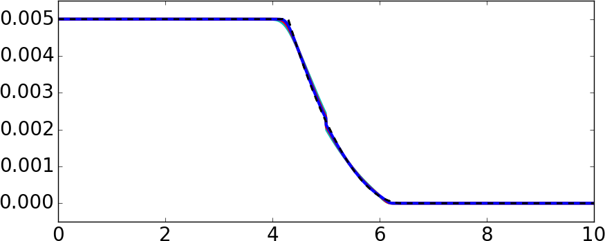
(d) Roe’s Riemann solver with $\lambda_{i\pm 1/2}^{\min}$.

Figure 1: Dam break problem over a dry bed using method (7) with different Riemann solvers. We show the numerical solution and the exact solution (in dashed black) at $t=10$. We consider different refinements with (cyan) $\Delta x=1/400$, (red) $\Delta x=1/800$, (blue) $\Delta x=1/1600$.

For this particular problem, using method (7) with the blended Riemann solver leads to $\lambda_{i\pm 1/2}^{\min}=0$ for all the experiments. We can artificially activate the entropy stabilization by imposing $\theta_{i}=0$ in (15), which is equivalent to using Roe’s solver with extra dissipation given by $\lambda_{i\pm 1/2}^{\min}$. In Figure 1d we show the solution, and in the last column of Table 1 we summarize the results of a convergence test. The entropy glitch is still noticeable but greatly reduced compared to the solution from Roe’s method without entropy stabilization. To remove completely the entropy glitch we could add high-order entropy dissipation following [41] and references therein.

	Roe’s solver		Rusanov’s solver		Blended solver		Roe’s with $\lambda_{i\pm 1/2}^{\min}$
$\Delta x$	$E_{1}$	rate	$E_{1}$	rate	$E_{1}$	rate	$E_{1}$	rate
1/50	6.21E-04	–	6.95E-04	–	5.08E-04	–	5.95E-04	–
1/100	4.70E-04	0.40	5.27E-04	0.40	3.39E-04	0.58	4.06E-04	0.55
1/200	3.91E-04	0.26	3.88E-04	0.44	2.30E-04	0.56	2.83E-04	0.52
1/400	3.16E-04	0.30	2.64E-04	0.55	1.49E-04	0.62	1.89E-04	0.58
1/800	2.35E-04	0.42	1.67E-04	0.66	9.24E-05	0.68	1.20E-04	0.65
1/1600	2.00E-04	0.23	1.01E-04	0.72	5.66E-05	0.70	7.42E-05	0.68

Table 1: Grid convergence study for the dam break problem over a dry bed using method (7) with different Riemann solvers.

4.2 Dam break problem on a wet bed

We consider now a one-dimensional dam break problem on a wet domain. We follow the setup in [8, §4.1.1]. The domain is $x\in(0,10)$ and the initial condition is given by $hu(x,0)=0$ and

$$h(x,0)=\begin{cases}h_{l}&x\leq x_{0}\\ h_{r}&x>x_{0}\end{cases}$$

with $x_{0}=5$, $h_{l}=0.005$, and $h_{r}=0.001$. The exact solution, which can be found in [8] and references therein, is given by

$$h(x,t)=\begin{cases}h_{l},\\ \frac{4}{9g}\left(\sqrt{gh_{l}}-\frac{x-x_{0}}{2t}\right)^{2},\\ \frac{c_{m}^{2}}{g},\\ h_{r},\end{cases}\quad u(x,t)=\begin{cases}0,&\mbox{ if }x\leq x_{A}(t),\\ \frac{2}{3}\left(\sqrt{gh_{l}}+\frac{x-x_{0}}{t}\right),&\mbox{ if }x_{A}(t)<x\leq x_{B}(t),\\ 2(\sqrt{gh_{l}}-c_{m}),&\mbox{ if }x_{B}(t)<x\leq x_{C}(t),\\ 0,&\mbox{ if }x<x_{C}(t),\end{cases}$$

where $x_{A}(t)=x_{0}-t\sqrt{gh_{l}}$, $x_{B}(t)=x_{0}+t\left(2\sqrt{gh_{l}}-3c_{m}\right)$, $x_{C}(t)=x_{0}+t\frac{2c_{m}^{2}\left(\sqrt{gh_{l}}-c_{m}\right)}{c_{m}^{2}-gh_{r}}$ and $c_{m}$ is the solution of $-8gh_{r}c_{m}^{2}\left(\sqrt{gh_{l}}-c_{m}\right)^{2}+\left(c_{m}^{2}-gh_{r}\right)^{2}\left(c_{m}^{2}+gh_{r}\right)=0$. We solve the problem up to the final time $t=5$ using the second-order method (3) with Roe’s, Rusanov’s and the blended solvers. The solution with different refinement levels and each Riemann solver is shown in Figure 2. In Table 2, we summarize the results of a convergence test. Since the solution is non-smooth, we expect no more than first order convergence rates. Note that the results with the entropy dissipative blended solver are comparable to the results using Roe’s solver. That is, imposing entropy dissipation via the blended Riemann solver does not degrade the high-order accuracy properties of Roe’s solver. In contrast, the accuracy and convergence rates using Rusanov’s solver are clearly degraded.

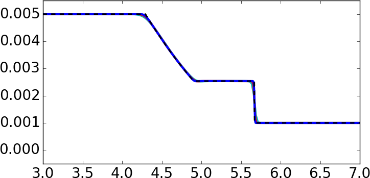
(a) Roe’s Riemann solver.

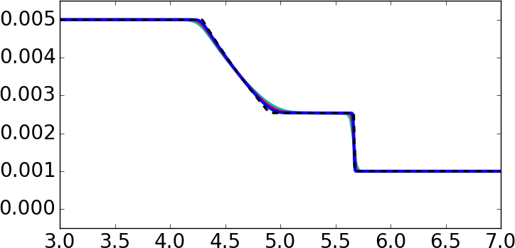
(b) Rusanov’s Riemann solver.

(c) Blended Riemann solver.

Figure 2: Dam break problem over a wet bed using method (3) with different Riemann solvers. We show the numerical solution and the exact solution (in dashed black) at $t=10$. We consider different refinements with (cyan) $\Delta x=1/400$, (red) $\Delta x=1/800$, (blue) $\Delta x=1/1600$.

	Roe’s solver		Rusanov’s solver		Blended solver
$\Delta x$	$E_{1}$	rate	$E_{1}$	rate	$E_{1}$	rate
1/50	4.22E-04	–	5.73E-04	–	4.24E-04	–
1/100	2.00E-04	1.07	3.35E-04	0.78	1.99E-04	1.08
1/200	1.11E-04	0.85	2.01E-04	0.74	1.10E-04	0.84
1/400	5.05E-05	1.13	1.18E-04	0.77	5.07E-05	1.12
1/800	2.60E-05	0.95	7.08E-05	0.74	2.61E-05	0.95
1/1600	1.29E-05	1.01	3.79E-05	0.90	1.29E-05	1.01

Table 2: Grid convergence study for the dam break problem over a wet bed using method (3) with different Riemann solvers.

4.3 Flow past a cylinder

In this section we consider the formation of a bow shock when a uniform flow encounters a cylindrical obstacle. This problem has been studied previously in the context of carbuncle formation in several works for the Euler equations and in [21, 2] for the shallow water equations. We present results for existing solvers as a form of verification, along with results for the new blended solver. The main question of interest is the formation of carbuncles. It is known, for instance, that the Roe solver incorrectly generates a carbuncle at the center of the bow shock.

We model only the flow on the upstream side of the cylinder, since our interest is in the resolution of the bow shock. We take the domain $[0,40]\times[0,100]$ with a cylinder of radius 20 centered at $(40,50)$. Reflecting boundary conditions are imposed at the surface of the cylinder, along with outflow conditions along the rest of the right edge of the domain. The depth and velocity are set initially and (for all time) at the other boundaries to $h_{0}=1$, $u_{0}=5$, for a Froude number of 5. We use a $160\times 400$ uniform Cartesian grid. In Figure 5, we show results at $t=80$, after the flow has reached a steady state. With Roe’s solver, negative values (of the water height) are generated at an early time, leading to failure of the solver. Therefore, we show results only for Rusanov’s, HLLEMCC by [21], and the blended solvers. These three methods give very similar results.

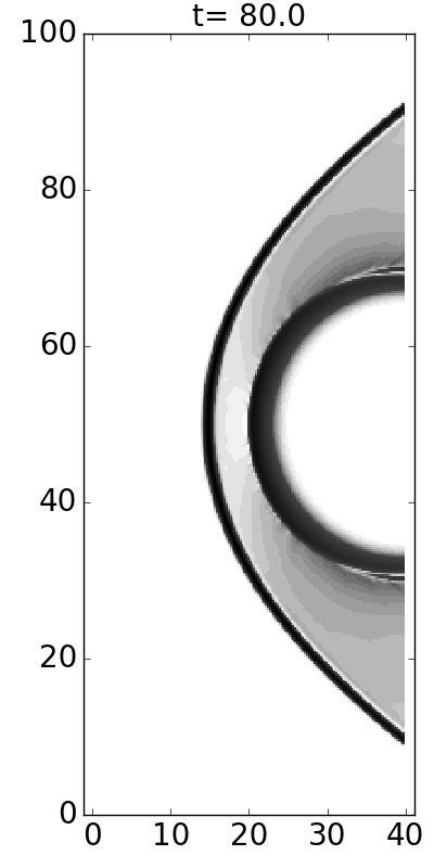
(a) Rusanov’s solver.

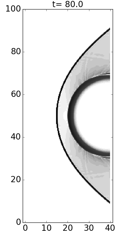
(b) HLLEMCC solver.

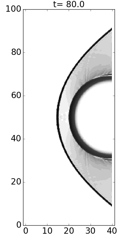
(c) Blended solver.

Figure 3: Flow past a cylinder. Results for Rusanov’s, HLLEMCC, and the blended solvers.

We have also conducted a more challenging version of this test, in which the velocity within the domain is initially zero. In that case, Rusanov’s and the blended solvers give carbuncle-free results similar to Figure 5, but HLLEMCC exhibits a carbuncle.

5 Numerical study of the circular hydraulic jump

5.1 Semi-analytical steady solution under rotational symmetry

In this section, we consider the initial boundary value problem consisting of the shallow water model (1) in an annular domain

$$r_{\textup{jet}}\leq r\leq r_{\infty}$$ (27)

where $r=\sqrt{x^{2}+y^{2}}$, with prescribed inflow at $r=r_{\textup{jet}}$ and prescribed outflow at $r=r_{\infty}$. The domain and boundary conditions are rotationally symmetric. By assuming rotational symmetry in (1), one obtains the system

$$(rh)_{t}+(rhu)_{r} =0,$$ (28a)

$$(rhu)_{t}+(rhu^{2})_{r}+r\left(\frac{1}{2}gh^{2}\right)_{r} =0,$$ (28b)

where the depth $h$ and radial velocity $u$ are functions of $r$ and $t$. By direct integration one finds that steady-state solutions of (28) satisfy

$$rhu =C$$ (29a)

$$h^{\prime}(r) =\frac{h(r)}{\frac{g}{\beta^{2}}r^{3}(h(r))^{3}-r}=\frac{h(r)}{r}\cdot\frac{(F(r))^{2}}{1-(F(r))^{2}}$$ (29b)

for some $C$ independent of $r$. Here $F(r)=|u(r)|/\sqrt{gh(r)}$ is the Froude number. We see that two types of steady profiles exist, depending on whether the flow is subcritical ($|F|<1$) or supercritical ($|F|>1$). No smooth steady solution can include both regimes, since the right hand side of (29b) blows up when $F=1$.

5.2 Numerical test: steady outflow

We now test the numerical methods by using a time-dependent simulation to compute the steady flow solution just described, in the annulus $r\in(0.1,1)$ with constant inflow at $r=0.1$ and outflow at $r=1$. The initial condition is $h(r,t=0)=0.1$, $hu(r,t=0)=0$, the inner boundary condition is $h(0.1,t)=0.3$, $hu(0.1,t)=0.75$, and the outer boundary condition is set to outflow (see [28, §21.8.5] for details). The computational mesh is logically quadrilateral, of the type shown in Figure 4.

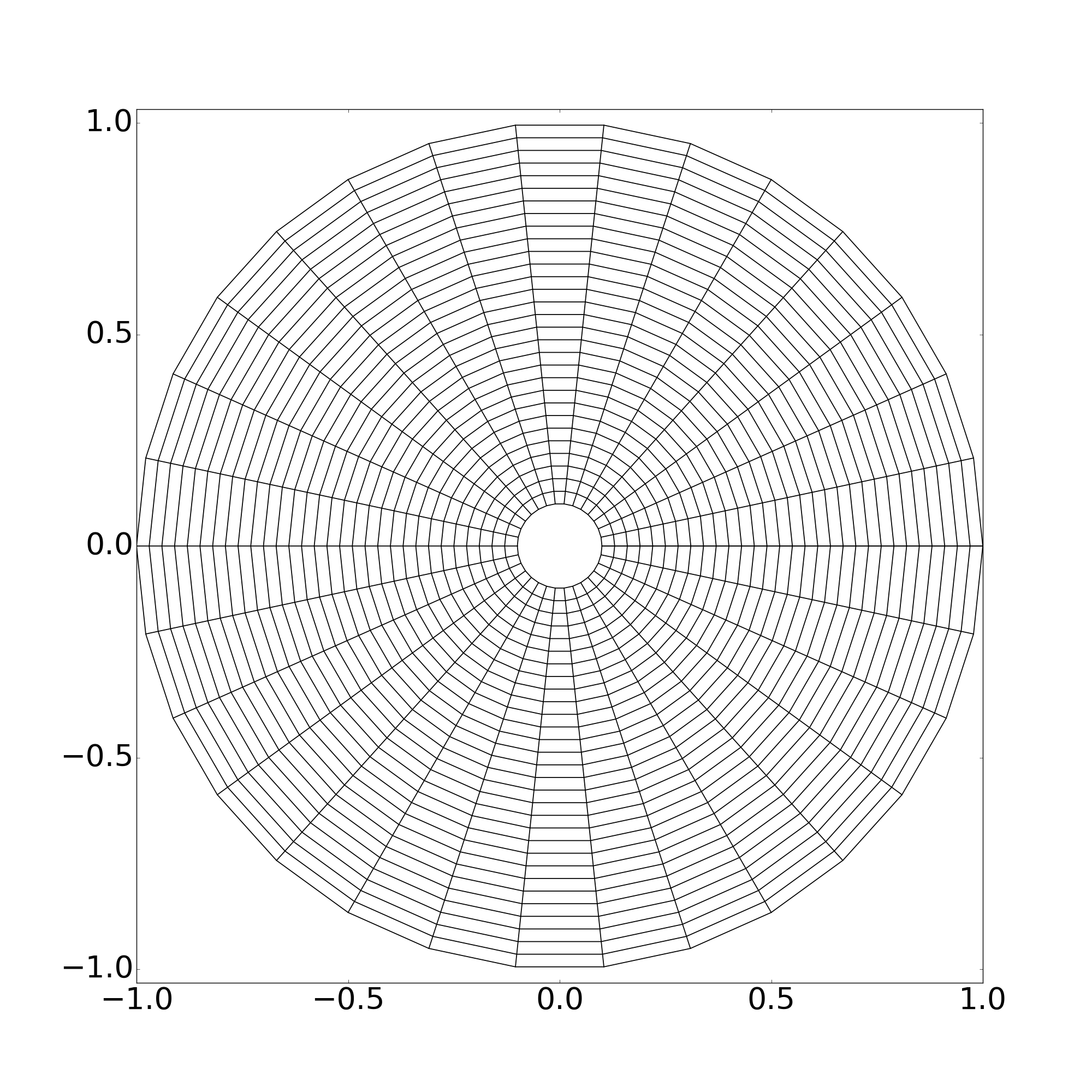
Figure 4: Example of a grid for the problem with the two-dimensional CHJ.

Regardless of the initial condition, the exact solution converges to a steady state profile given by one of the two solutions of (29), corresponding to subcritical or supercritical flow. In the present case we have imposed a supercritical inflow. In Figure 5, we show the solution and $\theta_{i}$ at different times using the second-order method (3) with Roe’s, Rusanov’s and the blended Riemann solvers. Additionally, in Table 3, we summarize the results of a convergence study based on methods (7) and (3), using the same Riemann solvers. Although the chosen initial condition leads initially to shock formation, the steady state is smooth and close to second order convergence is observed for the Roe and blended solvers.

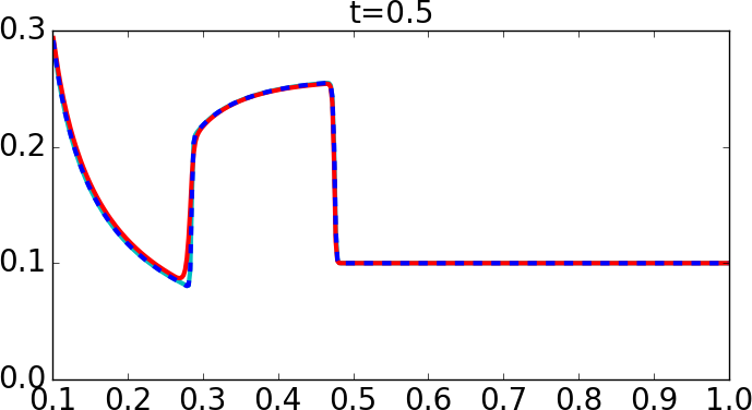
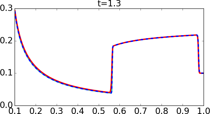
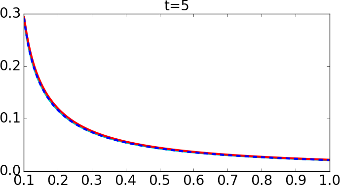
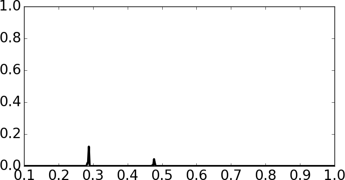
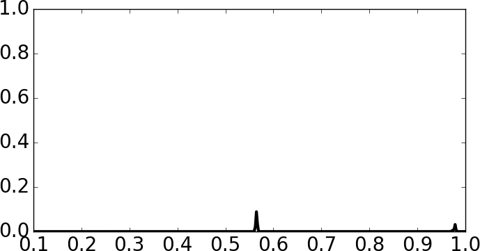
Figure 5: Steady outflow problem using method (3) with (cyan) Roe’s, (red) Rusanov’s and (dashed blue) the blended Riemann solvers. In the second row we plot $\theta_{i}$, which is given by (17). In all simulations we take $\Delta x=1/400$.

First-order method (7)

Second-order method (3)

Roe’s solver

Rusanov’s solver

Blended solver

Roe’s solver

Rusanov’s solver

Blended solver

$\Delta x$

$E_{1}$

rate

$E_{1}$

rate

$E_{1}$

rate

$E_{1}$

rate

$E_{1}$

rate

$E_{1}$

rate

1/50

2.16E-4

–

9.97E-4

–

2.16E-4

–

4.13E-5

–

7.32E-4

–

4.15E-5

–

1/100

1.14E-4

0.92

6.38E-4

0.64

1.14E-4

0.92

1.47E-5

1.48

4.43E-4

0.73

1.48E-5

1.48

1/200

5.86E-5

0.95

3.88E-4

0.72

5.87E-5

0.95

4.81E-6

1.61

2.57E-4

0.79

4.83E-6

1.61

1/400

2.98E-5

0.97

2.26E-4

0.78

2.98E-5

0.97

1.42E-6

1.76

1.44E-4

0.83

1.42E-6

1.76

1/800

1.50E-5

0.98

1.27E-4

0.83

1.50E-5

0.98

4.16E-7

1.76

7.81E-5

0.88

4.18E-7

1.76

1/1600

7.53E-6

0.99

6.90E-5

0.88

7.53E-6

0.99

1.14E-7

1.86

4.12E-5

0.92

1.15E-7

1.86

Table 3: Grid convergence study for the steady outflow problem using methods (7) and (3) with different Riemann solvers.

5.3 Location of the jump

The steady, rotationally-symmetric circular hydraulic jump involves supercritical flow for $r<r_{0}$ and subcritical flow for $r>r_{0}$, where $r_{0}$ is the jump radius. The jump itself takes the form of a stationary shock wave. The Rankine-Hugoniot jump conditions specify that for such a shock,

$$h_{+}-h_{-} =\frac{-3h_{-}+\sqrt{h_{-}^{2}+8h_{-}u_{-}^{2}/g}}{2}=\frac{3h_{-}}{2}\left(\sqrt{1+\frac{8}{9}(F_{-}^{2}-1)}-1\right),$$ (30)

where the subscripts $+,-$ denote states just inside or outside the jump radius, respectively.

A steady-state, rotationally symmetric solution can be given for an annular region with prescribed flow at the inner and outer boundaries as follows:

1. Specify the depth and velocity at the inner boundary (near the jet) and outer boundary.

2. Integrate (29b) from both boundaries.

3. Find a radius $r_{0}$ where the matching condition (30) is satisfied.

Due to the nature of solutions of (29b), it can be shown that the required jump radius $r_{0}$ always exists if the prescribed flow is supercritical at the inner boundary and subcritical at the outer boundary.

In this section we described how the location of the jump for a steady, rotationally-symmetric CHJ is determined by the boundary conditions. Following similar steps, one can choose inner boundary conditions and find outflow boundary conditions that lead to a CHJ at a prescribed location. This a convenient approach to construct initial conditions for numerical experiments at different flow regimes. Let us consider two flow regimes and construct the corresponding CHJs, which we use in the following sections. Consider the following boundary conditions:

$$h(x,y,t)=h_{\textup{jet}},\quad u(x,y,t)=|{u}_{\textup{jet}}|\left(\frac{x}{r_{\textup{jet}}}\right),\quad v(x,y,t)=|{u}_{\textup{jet}}|\left(\frac{y}{r_{\textup{jet}}}\right),\qquad\sqrt{x^{2}+y^{2}}=r_{\textup{jet}}$$ (31a)

$$h(x,y,t)=h_{\textup{out}},\quad u(x,y,t)=\frac{\beta}{r_{\textup{out}}h}\left(\frac{x}{r_{\textup{out}}}\right),\quad v(x,y,t)=\frac{\beta}{r_{\textup{out}}h}\left(\frac{y}{r_{\textup{out}}}\right),\qquad\sqrt{x^{2}+y^{2}}=r_{\textup{out}},$$ (31b)

where $h_{\textup{jet}}=0.3$, $r_{\textup{jet}}=0.1$, $r_{\textup{out}}=1$ and $\beta=r_{\textup{jet}}h_{\textup{jet}}|{u}_{\textup{jet}}|$. We choose $|{u}_{\textup{jet}}|$ and $h_{\textup{out}}$ such that the steady roationally-symmetric solution involves a symmetric shock at $r_{s}=0.3$; see Table 4. In Figure 6, we show the water depth $h$ along $y=0$ for these regimes.

	$F(r_{\textup{jet}})$	$|{u}_{\textup{jet}}|$	$h_{\textup{out}}$
Regime I	1.37	0.75	0.37387387318873766
Regime II	27.39	15	6.6845019298155357

Table 4: Boundary data $|u_{\textup{jet}}|$ and $h_{\textup{out}}$ which along with (31) produce CHJs located at $r_{s}=0.3$ for two different flow regimes.

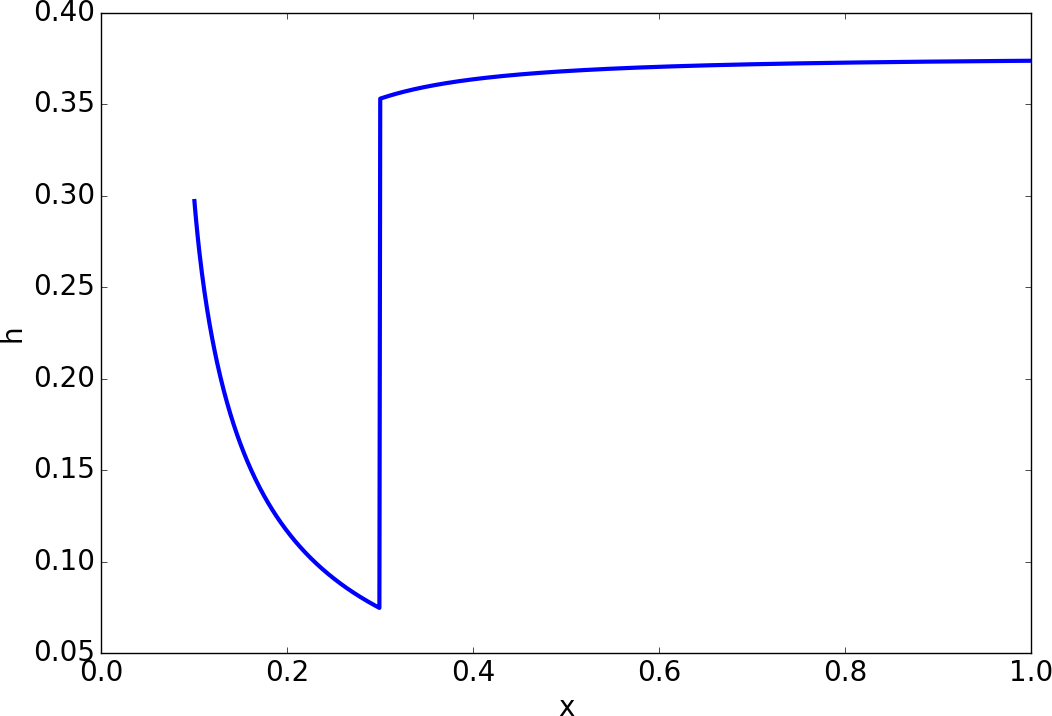
(a) $F(r_{\textup{jet}})\approx 1.37$

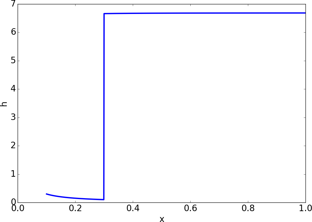
(b) $F(r_{\textup{jet}})\approx 27.39$

Figure 6: Radially symmetric CHJs created by solving (29) with a jump given by (30). We show a slice along $y=0$. In Section 5.4.1, we consider the CHJ in (a) as initial condition; and in Sections 5.4.2 and 5.4.3, we consider the CHJ in (b) as initial condition.

Numerical tests suggest that the solution of (28) rapidly approaches that just described under general initial conditions as long as the inflow at the jet is supercritical and the outflow at $r_{\infty}$ is subcritical. Subcritical outflow can be enforced by an appropriate outer boundary condition. This solution remains steady if the rate of inflow and outflow are matched. The stability of this solution in the face of non-rotationally-symmetric perturbations is an important question not only in the shallow water context but for more realistic fluid models and physically. It will play an important role in the results we present below. The rotationally-symmetric steady state is a useful initial condition for studies of CHJ stability.

5.4 The circular hydraulic jump in two dimensions

Let us finally consider the numerical experiments for the CHJ in two dimensions. The domain is again given by the annulus (27), but now we solve the fully 2D shallow water equations (1). For all of the following experiments, we use a mesh with 1000 cells in each (radial and angular) direction. The boundary conditions at the jet and the outer boundary are given by (31). By adjusting the boundary conditions $|{u}_{\textup{jet}}|$ and $h_{\textup{out}}$ we can study different flow regimes. We focus on the two cases in Table 4. For most of the experiments we show a Schlieren plot for the water height. That is, we plot $||\nabla h||_{\ell^{2}}$ with a greyscale logarithmic colormap.

5.4.1 Regime I ($F_{\textup{jet}}\approx 1.37$)

In this case, the boundary conditions are given by (31) with

$$|{u}_{\textup{jet}}|=0.75,\qquad h_{\textup{out}}=0.37387387318873766.$$ (32)

The initial condition is a circular hydraulic jump located at $r_{s}=0.3$; see Figure 6a. In Figure 7a, we show the solution at different times using method (3) with Roe’s Riemann solver. The solution clearly develops carbuncle instabilities, which are evident in the inset figure. In Figure 7b, we show solutions at $t=3$ for Rusanov’s, HLLEMCC, and the blended Riemann solvers. For this test case, these three solvers give qualitatively similar solutions, all of which are free from carbuncles.

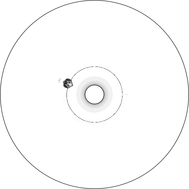
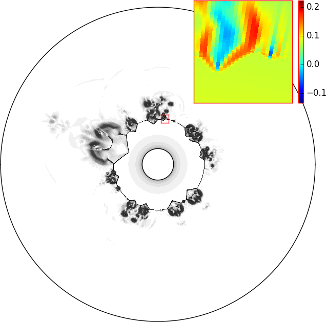
(a) Solution at (left) $t=1$, (middle) $t=1.5$ and (right) $t=3$ using Roe’s Riemann solver. The main plots are Schlieren plots of the depth $h$, while the inset in the right figure shows the momentum in the radial direction.

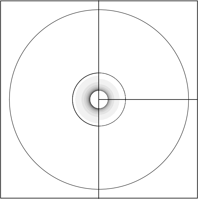
(b) Solution at $t=3$ using (left) Rusanov’s, (upper-right) HLLEMCC and (bottom-right) the blended solvers.

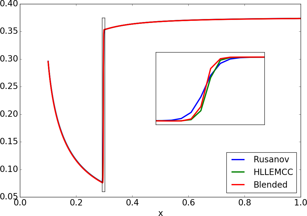
(c) Solution at $t=3$ along $y=0$ using the same solvers as in (b).

Figure 7: Simulation of a CHJ with boundary conditions given by (31) and (32). We consider method (3) with different Riemann solvers. In (a) and (b) we show the Schlieren plot for the water height $h$.

5.4.2 Regime II ($F_{\textup{jet}}\approx 27.39$)

We now consider a higher-Froude number regime. The boundary conditions are given by (31) with

$$|{u}_{\textup{jet}}|=15,\qquad h_{\textup{out}}=6.6845019298155357.$$ (33)

The initial condition is a circular hydraulic jump located at $r_{s}=0.3$; see Figure 6b. In Figure 8a, we show the solution at different times using method (3) with Roe’s Riemann solver. Again the solution develops carbuncle instabilities, which are clearly seen in the inset figure at $t=3$. For this regime, we obtained negative values for the water height with the HLLEMCC solver, which lead to failure of the solver. Therefore, in Figure 8b we only show results with Rusanov’s and the blended solvers.

The solutions obtained with these solvers show no carbuncles. The Rusanov solution remains very close to the initial symmetric equilibrium state, whereas the blended solver solution includes perturbations that appear just downstream from the jump. In Figure 9, we show the Rusanov and blended solutions at a much later time of $t=5$. In addition to the Schlieren plot of the water height, we superimpose a color plot of the magnitude of the momentum. It is evident that the visible perturbations in the blended solution are completely dissipated in the Rusanov solution, at least when using the grid employed here.

It is natural to ask whether these perturbations are meaningful; i.e., whether the symmetric equilibrium is unstable. To investigate this, we conduct one more test.

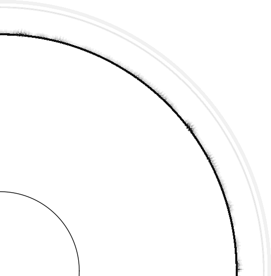
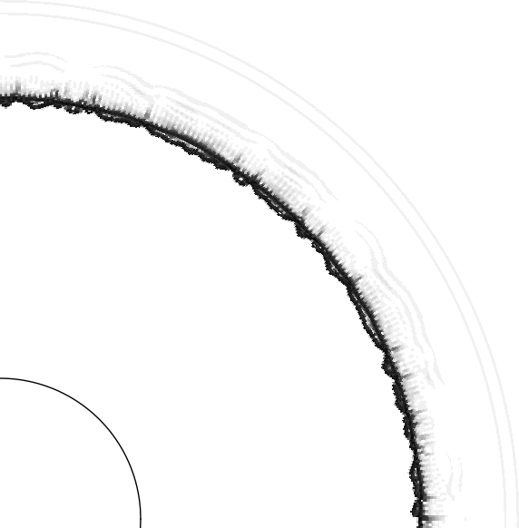
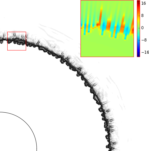
(a) Solution at (left) $t=0.09$, (middle) $t=0.1$ and (right) $t=0.11$ using Roe’s Riemann solver.

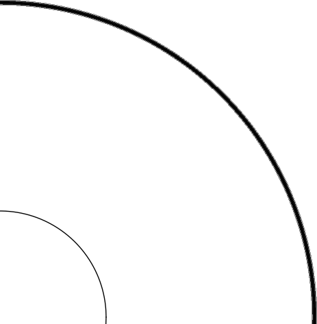
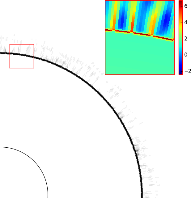
(b) Solution at $t=0.11$ using (left) Rusanov’s and (right) the blended solvers.

Figure 8: CHJ with boundary conditions given by (31) and (33). We consider method (3) with different Riemann solvers. In all cases we show the Schlieren plot for the water height $h$. The inset figures show the momentum in the radial direction.

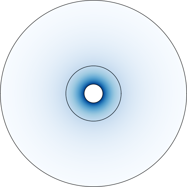
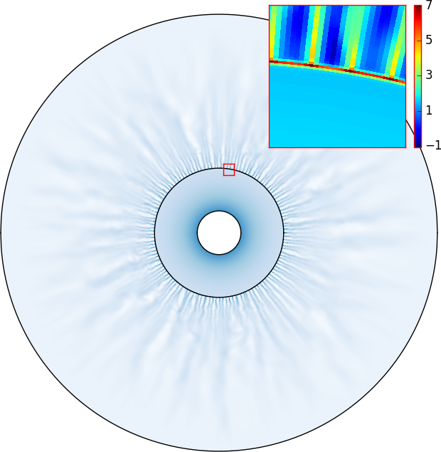
Figure 9: CHJ at $t=5$ with boundary conditions given by (31) and (33). We consider method (3) with (left) Rusanov’s and (right) the blended solvers. In all cases we superimpose the Schlieren plot for the water height $h$ an the magnitude of the momentum with a uniform (white-to-blue) colormap. The scale for colormap is (white) $0.45$ to (blue) $4.5$, which corresponds to the minimum and maximum values at $t=0$. The inset figure shows the momentum in the radial direction.

5.4.3 Regime II with random perturbations

Given the symmetry of the grid and initial data in the section above, the non-rotationally-symmetric perturbations seen when using the blended solver above must arise due to the influence of numerical errors. In order to understand whether these are evidence of a true instability, we now introduce a non-symmetric perturbation at the inflow boundary. We use the same mean values (33), but now we set

$$h(x,y,t)=\tilde{h}_{\textup{jet}},\quad u(x,y,t)=|\tilde{u}_{\textup{jet}}|\left(\frac{x}{r_{\textup{jet}}}\right),\quad v(x,y,t)=|\tilde{u}_{\textup{jet}}|\left(\frac{y}{r_{\textup{jet}}}\right),\qquad r=r_{\textup{jet}},$$ (34a)

with $\tilde{h}_{\textup{jet}}=\frac{h_{\textup{jet}}}{1+\epsilon(x,y,t)}$ and $|\tilde{u}_{\textup{jet}}|=|{u}_{\textup{jet}}|(1+\epsilon(x,y,t))$. Here $\epsilon(x,y,t)$ is chosen at each inflow boundary ghost cell and at each time step as an i.i.d. random variable from the uniform distribution $[-0.01,0.01]$. In this case, due to the large Froude number, the random perturbations in the inflow may trigger physical instabilities, which we want to preserve. At the same time, we do not want the solution to develop carbuncle instabilities. In figures 10a and 10b, we show the solution at different times considering method (3) with Rusanov’s and the blended Riemann solvers, respectively. In the right panel of Figure 10b, we show an inset figure with the momentum in the radial direction. Note that even though the solution is highly unstable (with the blended Riemann solver), no visible carbuncle instabilities are developed.

$t=2$	$t=3$	$t=4$	$t=5$

(a) Rusanov’s Riemann solver

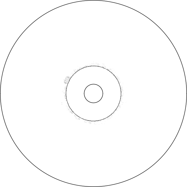
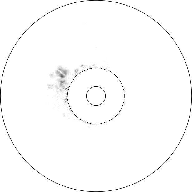
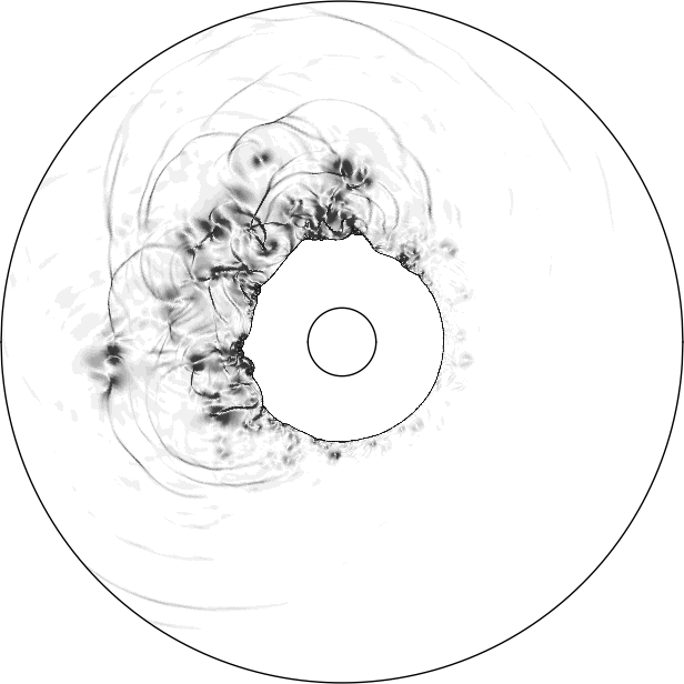
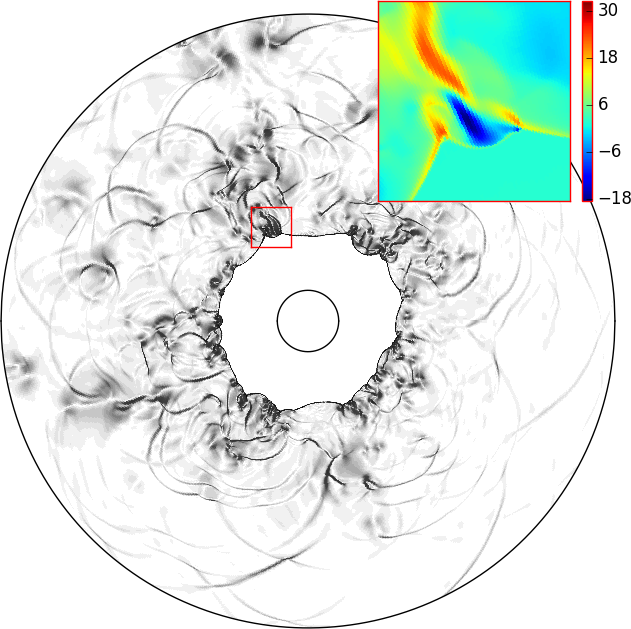
(b) Blended Riemann solver

Figure 10: CHJ at different times with a random perturbation at the inflow boundary. We consider method (3) with different Riemann solvers. In all cases we show the Schlieren plot for the water height $h$. The inset figure shows the momentum in the radial direction.

6 Conclusions

In this work we have introduced a new Riemann solver for the shallow water equations, described in Section 3. Through numerical tests we have shown that the solver gives accuracy similar to that of Roe’s method and robustness similar to that of Rusanov’s method. Although the full second-order method we have proposed is not provably entropy stable or positivity preserving, it gives improved results for test problems where both of these properties are important. The approach used in Section 3 could be applied to enforce entropy stability for any Riemann solver of the type used in Clawpack. The same techniques could also be used more generally to avoid carbuncles in the solution of the Euler equations.

We have introduced two new test problems for numerical shallow water solvers, both consisting of flow in an annulus, with inflow from a jet at the center and outflow at the outer boundary. The first test problem, described in Section 5.2, has a smooth solution that can be computed by solving an ODE and thus serves as a useful test of accuracy. The second problem, the circular hydraulic jump, involves a standing shock wave that can be physically unstable but is also susceptible to the numerical carbuncle instability. Additionally, it involves high-velocity low-depth flow regions where it is challenging to maintain positivity. This makes it an excellent problem for testing that schemes are both robust and not overly dissipative.

Acknowledgment. We thank Prof. Friedemann Kemm for sharing helpful code with us and for reviewing an early version of this manuscript.

References

- [1] Pascal Azerad, Jean-Luc Guermond, and Bojan Popov. Well-balanced second-order approximation of the shallow water equation with continuous finite elements. SIAM Journal on Numerical Analysis, 55(6):3203–3224, 2017.
- [2] Georg Bader and Friedemann Kemm. The carbuncle phenomenon in shallow water simulations. In The second international conference on computational science and engineering (ICCSE-2014). Ho Chi Minh City, Vietnam, 2014.
- [3] Tomas Bohr, Peter Dimon, and Vakhtang Putkaradze. Shallow-water approach to the circular hydraulic jump. Journal of Fluid Mechanics, 254:635–648, 1993.
- [4] John WM Bush and Jeffrey M Aristoff. The influence of surface tension on the circular hydraulic jump. Journal of Fluid Mechanics, 489:229–238, 2003.
- [5] Yann Chauvat, J-M Moschetta, and Jérémie Gressier. Shock wave numerical structure and the carbuncle phenomenon. International Journal for Numerical Methods in Fluids, 47(8-9):903–909, 2005.
- [6] Clawpack Development Team. Clawpack software, 2020. Version 5.7.1.
- [7] ADD Craik, RC Latham, MJ Fawkes, and PWF Gribbon. The circular hydraulic jump. Journal of Fluid Mechanics, 112:347–362, 1981.
- [8] Olivier Delestre, Carine Lucas, Pierre-Antoine Ksinant, Frédéric Darboux, Christian Laguerre, T-N-Tuoi Vo, Francois James, and Stéphane Cordier. Swashes: a compilation of shallow water analytic solutions for hydraulic and environmental studies. International Journal for Numerical Methods in Fluids, 72(3):269–300, 2013.
- [9] Xi Deng, Pierre Boivin, and Feng Xiao. A new formulation for two-wave Riemann solver accurate at contact interfaces. Physics of Fluids, 31(4):046102, 2019.
- [10] Michael Dumbser, Jean-Marc Moschetta, and Jérémie Gressier. A matrix stability analysis of the carbuncle phenomenon. Journal of Computational Physics, 197(2):647–670, 2004.
- [11] Clive Ellegaard, Adam Espe Hansen, Anders Haaning, Kim Hansen, Anders Marcussen, Tomas Bohr, Jonas Lundbek Hansen, and Shinya Watanabe. Creating corners in kitchen sinks. Nature, 392(6678):767, 1998.
- [12] Volker Elling. The carbuncle phenomenon is incurable. Acta Mathematica Scientia, 29(6):1647–1656, 2009.
- [13] Alexandre Ern and Jean-Luc Guermond. Weighting the edge stabilization. SIAM Journal on Numerical Analysis, 51(3):1655–1677, 2013.
- [14] Jean-Luc Guermond, Manuel Quezada de Luna, Bojan Popov, Christopher E Kees, and Matthew W Farthing. Well-balanced second-order finite element approximation of the shallow water equations with friction. SIAM Journal on Scientific Computing, 40(6):A3873–A3901, 2018.
- [15] Jean-Luc Guermond, Murtazo Nazarov, Bojan Popov, and Ignacio Tomas. Second-order invariant domain preserving approximation of the Euler equations using convex limiting. SIAM Journal on Scientific Computing, 40(5):A3211–A3239, 2018.
- [16] Jean-Luc Guermond, Richard Pasquetti, and Bojan Popov. Entropy viscosity method for nonlinear conservation laws. Journal of Computational Physics, 230(11):4248–4267, 2011.
- [17] Seikan Ishigai, Shigeyasu Nakanishi, Minoru Mizuno, and Toyoo Imamura. Heat transfer of the impinging round water jet in the interference zone of film flow along the wall. Bulletin of JSME, 20(139):85–92, 1977.
- [18] Farzad Ismail and Philip L Roe. Affordable, entropy-consistent Euler flux functions II: Entropy production at shocks. Journal of Computational Physics, 228(15):5410–5436, 2009.
- [19] Farzad Ismail, Philip L Roe, and Hiroaki Nishikawa. A proposed cure to the carbuncle phenomenon. In Computational Fluid Dynamics 2006, pages 149–154. Springer, 2009.
- [20] S Jaisankar and SV Raghurama Rao. Diffusion regulation for Euler solvers. Journal of Computational Physics, 221(2):577–599, 2007.
- [21] Friedemann Kemm. A note on the carbuncle phenomenon in shallow water simulations. ZAMM-Journal of Applied Mathematics and Mechanics/Zeitschrift für Angewandte Mathematik und Mechanik, 94(6):516–521, 2014.
- [22] David I Ketcheson, Randall J LeVeque, and Mauricio J del Razo. Riemann Problems and Jupyter Solutions, volume 16. SIAM, 2020.
- [23] David I. Ketcheson, Kyle T. Mandli, Aron J. Ahmadia, Amal Alghamdi, Manuel Quezada de Luna, Matteo Parsani, Matthew G. Knepley, and Matthew Emmett. PyClaw: Accessible, Extensible, Scalable Tools for Wave Propagation Problems. SIAM Journal on Scientific Computing, 34(4):C210–C231, November 2012.
- [24] M Kurihara. On hydraulic jumps. Proceedings of the Report of the Research Institute for Fluid Engineering, Kyusyu Imperial University, 3(2):11–33, 1946.
- [25] Dmitri Kuzmin and Manuel Quezada de Luna. Algebraic entropy fixes and convex limiting for continuous finite element discretizations of scalar hyperbolic conservation laws. Computer Methods in Applied Mechanics and Engineering, 372:113370, 2020.
- [26] Dmitri Kuzmin and Manuel Quezada de Luna. Entropy conservation property and entropy stabilization of high-order continuous galerkin approximations to scalar conservation laws. Computers & Fluids, 213:104742, 2020.
- [27] Randall J LeVeque. Wave propagation algorithms for multidimensional hyperbolic systems. Journal of computational physics, 131(2):327–353, 1997.
- [28] Randall J LeVeque et al. Finite volume methods for hyperbolic problems, volume 31. Cambridge university press, 2002.
- [29] J-M Moschetta, J Gressier, J-C Robinet, and G Casalis. The carbuncle phenomenon: a genuine Euler instability? In Godunov Methods, pages 639–645. Springer, 2001.
- [30] Hiroaki Nishikawa and Keiichi Kitamura. Very simple, carbuncle-free, boundary-layer-resolving, rotated-hybrid Riemann solvers. Journal of Computational Physics, 227(4):2560–2581, 2008.
- [31] Taku Ohwada, Yuki Shibata, Takuma Kato, and Taichi Nakamura. A simple, robust and efficient high-order accurate shock-capturing scheme for compressible flows: Towards minimalism. Journal of Computational Physics, 362:131–162, 2018.
- [32] Maurizio Pandolfi and Domenic D’Ambrosio. Numerical instabilities in upwind methods: analysis and cures for the “carbuncle” phenomenon. Journal of Computational Physics, 166(2):271–301, 2001.
- [33] K Peery and S Imlay. Blunt-body flow simulations. In 24th Joint Propulsion Conference, page 2904, 1988.
- [34] James J Quirk. A contribution to the great Riemann solver debate. In Upwind and High-Resolution Schemes, pages 550–569. Springer, 1997.
- [35] Deep Ray and Praveen Chandrashekar. Entropy stable schemes for compressible Euler equations. Int. J. Numer. Anal. Model. Ser. B, 4(4):335–352, 2013.
- [36] Lord Rayleigh. On the theory of long waves and bores. Proceedings of the Royal Society of London. Series A, Containing Papers of a Mathematical and Physical Character, 90(619):324–328, 1914.
- [37] Zhijun Shen, Wei Yan, and Guangwei Yuan. A stability analysis of hybrid schemes to cure shock instability. Communications in Computational Physics, 15(5):1320–1342, 2014.
- [38] Sangeeth Simon. Numerical Shock Instability In HLL-Based Approximate Riemann Solvers For The Euler System Of Equations: Analysis And Cures. PhD thesis, Indian Institute of Technology Bombay Mumbai 400076 (India.
- [39] Gilbert Strang. On the construction and comparison of difference schemes. SIAM journal on numerical analysis, 5(3):506–517, 1968.
- [40] Eitan Tadmor. The numerical viscosity of entropy stable schemes for systems of conservation laws. I. Mathematics of Computation, 49(179):91–103, 1987.
- [41] Eitan Tadmor. Entropy stability theory for difference approximations of nonlinear conservation laws and related time-dependent problems. Acta Numerica, 12(1):451–512, 2003.
- [42] Itiro Tani. Water jump in the boundary layer. Journal of the Physical Society of Japan, 4(4-6):212–215, 1949.
- [43] Dongfang Wang, Xiaogang Deng, Guangxue Wang, and Yidao Dong. Developing a hybrid flux function suitable for hypersonic flow simulation with high-order methods. International Journal for Numerical Methods in Fluids, 81(5):309–327, 2016.
- [44] EJ Watson. The radial spread of a liquid jet over a horizontal plane. Journal of Fluid Mechanics, 20(3):481–499, 1964.