dummy

1 Introduction

Heavy-ion experiments at RHIC and LHC have produced convincing evidence that a Quark-Gluon Plasma (QGP) is formed in high-energy nucleus-nucleus ($\mathrm{A}\mathrm{A}$) collisions. The discussion therefore has developed into one of understanding the underlying detailed mechanisms, such as the nature of the initial state, the early thermalization, the subsequent hydrodynamical expansion, and the transition back to a hadronic state. Numerous models have been and are being developed to study such issues.

The standard picture of heavy ion collisions, separates the evolution of the QGP phase into three or four stages, outlined in the following.

The first $<1$ fm after the collision, is denoted the “initial state”. It consists of dense matter, highly out of equilibrium. Most QGP-based models seek to calculate an energy density (or a full energy-momentum tensor) from a model of the evolution of the initial stage. The simplest approaches are based purely on geometry, and are denoted Glauber models [1]. Here, the energy density in the transverse plane is determined purely from the distributions of nucleons in the incoming nuclei. Going beyond nucleonic degrees of freedom, some of the more popular choices includes either introducing constituent quarks [2], or invoking the more involved formalism known the Colour Glass Condensate [3]. In the latter case, the so-called IP-Glasma [4] program is often used, as it allows for computations with realistic boundary conditions.

The initial state, glasma or not, will then transition into a plasma. Recently, progress has been made to describe the transition from an out-of-equilibrium initial state to a hydrodynamized plasma, using kinetic theory [5]. In such cases, the pre-equilibration will describe the dynamics between $\approx 0.1-1$ fm.

Between $1-10$ fm, the plasma evolves according to relativistic viscous hydrodynamics [6, 7, 8]. Hydrodynamics is a long wavelength effective theory, able to describe interactions at low momentum, when the mean free path of particles is much smaller than the characteristic size of the system. As such, its use has been criticised in small collision systems, but nevertheless seems to be able to describe flow observables reasonably well even there [9].

Finally, after 10 fm, the QGP freezes out to hadronic degrees of freedom. The physics involved after this freeze-out is the main topic of this paper, though with the large difference to traditional approaches, that it happens much sooner.

Paradoxically, one of the key problems is that the QGP picture has been too successful. QGP formation was supposed to be unique to $\mathrm{A}\mathrm{A}$ collisions, while $\mathrm{p}\mathrm{A}$ and $\mathrm{p}\mathrm{p}$ collisions would not involve volumes and time scales large enough for it. And yet QGP-like signals have been found in these as well. One key example is the observation of a non-isotropic particle flow, in the form of a “ridge” at the same azimuthal angle as a trigger jet [10, 11, 12] or of non-vanishing $v_{2}$ azimuthal flow coefficients [11, 12, 13]. Another example is that the fraction of strange hadrons, and notably multi-strange baryons, is smoothly increasing from low-multiplicity to high-multiplicity $\mathrm{p}\mathrm{p}$, on through $\mathrm{p}\mathrm{A}$ to saturate for $\mathrm{A}\mathrm{A}$ multiplicities [14].

The most obvious way out is to relax the large-volume requirement, and accept that a QGP, or at least a close-to-QGP-like state, can be created in smaller systems. An excellent example of this approach is the core–corona model [15], implemented in the EPOS event generator [16], wherein the high-density core of a system hadronizes like a plasma, while the outer lower-density corona does not. The evolution from low-multiplicity $\mathrm{p}\mathrm{p}$ to $\mathrm{A}\mathrm{A}$ is then a consequence of an increasing core fraction.

Another approach is to ask what physics mechanisms, not normally modelled in $\mathrm{p}\mathrm{p}$ collisions, would be needed to understand $\mathrm{p}\mathrm{p}$ data without invoking QGP formation. And, once having such a model, one could ask what consequences that would imply for $\mathrm{p}\mathrm{A}$ and $\mathrm{A}\mathrm{A}$ collisions. More specifically, could some of the signals attributed to QGP formation have alternative explanations? If nothing else, exploring these questions could help sharpen experimental tests, by providing a straw-man model. At best, we may actually gain new insights.

This is the road taken by the Angantyr model [17, 18]. It is based on and contained in the Pythia event generator [19, 20], which successfully describes many/most features of LHC $\mathrm{p}\mathrm{p}$ events. Angantyr adds a framework wherein $\mathrm{p}\mathrm{A}$ and $\mathrm{A}\mathrm{A}$ collisions can be constructed as a superposition of simpler binary collisions, in the spirit of the old Fritiof model [21, 22]. Such a framework is already sufficient to describe many simple $\mathrm{p}\mathrm{A}$ and $\mathrm{A}\mathrm{A}$ distributions, such as $\mathrm{d}n_{\mathrm{charged}}/\mathrm{d}\eta$. Beyond that, it also offers a platform on top of which various collective non-QGP phenomena can be added. One example is shoving [23, 24, 25], whereby closely overlapping colour fields repel each other, to give a collective flow. Another is colour rope formation [26], wherein overlapping colour fields can combine to give a higher field strength, thus enhancing strangeness production relative to the no-overlap default.

In this article we will study a third mechanism, that of hadronic rescattering. The basic idea here is that the standard fragmentation process produces a region of closely overlapping hadrons, that then can collide with each other as the system expands. Each single such collision on its own will give negligible effects, but if there are many of them then together they may give rise to visible physics signals. Rescattering is often used as an afterburner to the hadronization of the QGP, commonly making use of the UrQMD [27] or SMASH [28] programs. What makes Angantyr/Pythia different is that there is no QGP phase, so that rescattering can start earlier, and therefore hypothetically can give larger effects. In order to use a rescattering framework as an afterburner to Angantyr, a first step is to describe the space–time structure of hadronization in Pythia, which was worked out in [29]. This picture can easily be extended from $\mathrm{p}\mathrm{p}$ to $\mathrm{p}\mathrm{A}$ and $\mathrm{A}\mathrm{A}$ using the nuclear geometry set up in Angantyr. Thereby the road is open to add rescattering eg. with UrQMD, which was done by Ref. [30].

Using two different programs is cumbersome, however. It requires the user to learn to use each individual framework, and they have to convert the output from the first program into a format that can be input to the second. A related issue arises if the two programs represent event records differently, so that it might be impossible to trace the full particle history. A desire for convenience is one of the main motivations behind a recently developed framework for hadronic rescattering, implemented natively in Pythia [31]. With this framework, rescattering can be enabled with just a single additional line of code, which is a trivial task for anyone already familiar with Pythia. In addition, this framework also introduces physics features not found in some other frameworks, such as a basic model for charm and bottom hadrons in rescattering, and with Pythia being in active development, there is a low threshold for making further improvements in the future.

In [31], initial studies using the framework were limited to implications for $\mathrm{p}\mathrm{p}$ collisions, which not unexpectedly were found to be of moderate size. That is, while visible enough in model studies, generally they are less easy to pin down experimentally, given all other uncertainties that also exist. In this article the rescattering studies are extended to $\mathrm{p}\mathrm{A}$ and $\mathrm{A}\mathrm{A}$ collisions, where effects are expected to be larger. Indeed, as we shall see, the outcome confirms this expectation. The number of rescatterings rises faster than the particle multiplicity, such that the fraction of not-rescattered hadrons is small in $\mathrm{PbPb}$ collisions. Rescatterings are especially enhanced at lower masses, but the process composition at a given mass is universal. Obviously the primary production volume increases from $\mathrm{p}\mathrm{p}$ and $\mathrm{p}\mathrm{A}$ to $\mathrm{A}\mathrm{A}$, and thus so does the range of rescatterings. Transverse momentum spectra are significantly more deformed by rescattering in $\mathrm{A}\mathrm{A}$. There is a clear centrality dependence on particle production rates, eg. a $\mathrm{J}/\psi$ depletion in central collisions. The most interesting result is a clear signal of elliptic flow induced by rescatterings, that even matches experimental $\mathrm{PbPb}$ numbers at large multiplicities, to be contrasted with the miniscule effects in $\mathrm{p}\mathrm{p}$.

The outline of the article is as follows. In Section 2 we describe the main points of the model, from the simulation of the nuclear collision, through the modelling of individual nucleon–nucleon sub-collisions and on to the rescattering framework proper. In Section 3 effects in this model are tested on its own, while Section 4 shows comparisons with data. Some conclusions and an outlook are presented in Section 5. Finally, technical aspects related to computation time for rescattering are discussed in the appendix.

Natural units are assumed throughout the article, ie. $c=\hbar=1$. Energy, momentum and mass are given in GeV, space and time in fm, and cross sections in mb.

2 The model

In this section we will review the framework used to simulate nuclear collisions. Initially the Angantyr framework is used to set the overall nucleus–nucleus ($\mathrm{A}\mathrm{A}$) collision geometry and select colliding nucleon-nucleon ($\mathrm{N}\mathrm{N}$) pairs. Then the Multiparton Interactions (MPI) concept is used to model each single $\mathrm{N}\mathrm{N}$ collision. The resulting strings are fragmented to provide the primary setup of hadrons, that then can begin to decay and rescatter. All of these components are described in separate publications, where further details may be found, so only the key aspect are collected here is to describe how it all hangs together.

2.1 ANGANTYR

The Angantyr part of the modelling is responsible for setting up the $\mathrm{A}\mathrm{A}$ collision geometry, and selecting the number and nature of the ensuing $\mathrm{N}\mathrm{N}$ collisions [18].

Take the incoming high-energy nucleons to be travelling along the $\pm z$ directions. By Lorentz contraction all the $\mathrm{N}\mathrm{N}$ collisions then occur in a negligibly small range around $t=z=0$, and the nucleon transverse $(x,y)$ positions can be considered frozen during that time. The nucleon locations inside a nucleus are sampled according to a two-dimensional Woods-Saxon distribution in the GLISSANDO parametrisation [32, 33], applicable for heavy nuclei with $A>16$, and with a nuclear repulsion effect implemented algorithmically as a “hard core” radius of each nucleon, below which two nucleons cannot overlap. The $\mathrm{A}\mathrm{A}$ collision impact parameter provides an offset $\pm b_{\mathrm{A}\mathrm{A}}/2$, eg. along the $x$ axis. Up to this point, this is a fairly standard Glauber model treatment, where one would then combine the geometry with measured cross sections (usually total and/or inelastic non-diffractive), to obtain the amount of participating or wounded nucleons, and the number of binary sub-collisions (see eg. Ref. [1] for a review). In Angantyr, a distinction between nucleons wounded inelastic non-diffractively, diffractively or elastically is desired, along with a dependence on the nucleon-nucleon impact parameter. To this end, a parametrization of the nucleon-nucleon elastic amplitude in impact parameter space ($T(\vec{b})$) is used. It allows for the calculation of the amplitude $T_{kl}(\vec{b})$ for any combination of projectile and target state, $k$ and $l$ respectively. All parameters of the parametrization can be estimated from proton-proton total and semi-inclusive cross sections, and varies with collision energy. The input cross sections used are the ones available in Pythia, with the SaS model [34] being the default choice. The parametrization of $T(\vec{b})$ thus adds no new parameters beyond the ones already present in the model for hadronic cross sections.

Inelastic non-diffractive collisions involve a colour exchange between two nucleons. In the simplest case, where each incoming nucleon undergoes at most one collision, the traditional Pythia collision machinery can be used essentially unchanged. The one difference is that the nuclear geometry has already fixed the $\mathrm{N}\mathrm{N}$ impact parameter $b_{\mathrm{N}\mathrm{N}}$, whereas normally this would be set only in conjunction with the hardest MPI.

The big extension of Angantyr is that it also handles situations where a given nucleon $A$ interacts inelastic non-diffractively with several nucleons $B_{1},B_{2},\ldots B_{n}$ from the other nucleus. Colour fields would then be stretched from $A$ to each $B_{i}$. It would be rare for all the fields to stretch all the way out to $A$, however, but rather matching colour–anticolour pairs would “short-circuit” most of the colour flow out to the remnants. Such a mechanism is already used for MPIs in a single $\mathrm{N}\mathrm{N}$ collision, but here it is extended to the full set of interconnected nucleons. Therefore only one $AB_{i}$ collision is handled as a normal $\mathrm{N}\mathrm{N}$ one, while the other $AB_{j},j\neq i$ ones will produce particles over a smaller rapidity range. This is analogous to the situation encountered in single diffraction $AB_{j}\to AX_{j}$. If we further assume that the short-circuiting can occur anywhere in rapidity with approximately flat probability distribution, this translates into an excited mass spectrum like $\mathrm{d}M_{X_{j}}^{2}/M_{X_{j}}^{2}$, again analogous to diffraction. To this end, $n-1$ carrier particles with vacuum quantum numbers $\mathbb{P}_{j}$ (denoted $\mathbb{P}$ for the similarity with pomerons) are emitted, with fractions $x_{j}$ of the incoming $A$ (lightcone) momentum picked according to $\mathrm{d}x_{j}/x_{j}$, subject to momentum conservation constraints, with a leftover $x_{i}$ that usually should represent the bulk of the $A$ momentum. Thereby the complexity of the full problem is reduced to one of describing one regular $AB_{i}$ collision, at a slightly reduced energy, and $n-1$ $\mathbb{P}_{j}B_{j}$ collisions, at significantly reduced energies, similar to diffraction. The pomeron-like objects have no net colour or flavour, but they do contain partons and the full MPI machinery can be applied to describe also these collisions. As the particles are not true pomerons, the PDFs can be different from the pomeron ones measured at HERA, and the transverse size is that of the original nucleon rather than the smaller one expected for a pomeron.

In a further step of complexity, the nucleons on side $A$ and $B$ may be involved in multiply interrelated chains of interactions. Generalizing the principles above, it is possible to reduce even complex topologies to a set of decoupled $\mathrm{N}\mathrm{N}$, $\mathrm{N}\mathbb{P}$, and $\mathbb{P}\mathbb{P}$ collisions, to be described below. The reduction is not unique, but may be chosen randomly among the allowed possibilities.

One current limitation is that there is no description of the breakup of the nuclear remnant. Rather, all non-wounded nucleons of a nucleus are collected together into a single fictitious new nucleus, that is not considered any further.

2.2 Multiparton interaction vertices

At the end of the Angantyr modelling, a set of separate hadron–hadron ($\mathrm{H}\mathrm{H}$) interactions have been defined inside an $\mathrm{A}\mathrm{A}$ collision, where the hadron can be either a nucleon or a pomeron-like object as discussed above. The locations of the $\mathrm{H}\mathrm{H}$ collisions in the transverse plane is also fixed.

When two Lorentz-contracted hadrons collide inelastically with each other, a number of separate (semi-)perturbative parton–parton interactions can occur. These are modelled in a sequence of falling transverse momenta $p_{\perp}$, as described in detail elsewhere [35, 36]. The MPI vertices are spread over a transverse region of hadronic size, but in the past it was not necessary to assign an explicit location for every single MPI. Now it is. The probability for an interaction at a given transverse coordinate $(x,y)$ can be assumed proportional to the overlap of the parton densities of the colliding hadrons in that area element. A few possible overlap function options are available in Pythia, where the Gaussian case is the simplest one. If two Gaussian-profile hadrons pass with an impact parameter $b_{\mathrm{H}\mathrm{H}}$, then the nice convolution properties gives a total overlap that is a Gaussian in $b_{\mathrm{H}\mathrm{H}}$, and the distribution of MPI vertices is a Gaussian in $(x,y)$. Specifically note that there is no memory of the collision plane in the vertex distribution.

This property is unique to Gaussian convolutions, however. In general, the collision region will be elongated either out of or in to the collision plane. The former typically occurs for a distribution with a sharper proton edge, eg. a uniform ball, which gives rise to the almond-shaped collision region so often depicted for heavy-ion collisions. The latter shape instead occurs for distributions with a less pronounced edge, such as an exponential. The default Pythia behaviour is close to Gaussian, but somewhat leaning towards the latter direction. Even that is likely to be a simplification. The evolution of the incoming states by initial-state cascades is likely to lead to “hot spots” of increased partonic activity, see eg. [37]. A preliminary study in [31] showed that azimuthal anisotropies in the individual $\mathrm{H}\mathrm{H}$ collision give unambiguous, but miniscule flow effects, and furthermore the many $\mathrm{H}\mathrm{H}$ event planes of an $\mathrm{A}\mathrm{A}$ collision point in random directions, further diluting any such effects. In the end, it is the asymmetries related to the $\mathrm{A}\mathrm{A}$ geometry that matter for our studies.

Only a fraction of the full nucleon momentum is carried away by the MPIs of an $\mathrm{H}\mathrm{H}$ collision, leaving behind one or more beam remnants [38]. These are initially distributed according to a Gaussian shape around the center of the respective hadron. By the random fluctuations, and by the interacting partons primarily being selected on the side leaning towards the other beam hadron, the “center of gravity” will not agree with the originally assumed origin. All the beam remnants will therefore be shifted so as to ensure that the energy-weighted sum of colliding and remnant parton locations is where it should be. Shifts are capped to be at most a proton radius, so as to avoid extreme spatial configurations, at the expense of a perfectly aligned center of gravity.

Not all hadronizing partons are created in the collision moment $t=0$. Initial-state radiation (ISR) implies that some partons have branched off already before this, and final-state radiation (FSR) that others do it afterwards. These partons then can travel some distance out before hadronization sets in, thereby further complicating the space–time picture, even if the average time of parton showers typically is a factor of five below that of string fragmentation [29]. We do not trace the full shower evolution, but instead include a smearing of the transverse location in the collision plane that a parton points back to. No attempt is made to preserve the center of gravity during these fluctuations.

The partons produced in various stages of the collision process (MPIs, ISR, FSR) are initially assigned colours according to the $N_{C}\to\infty$ approximation, such that different MPI systems are decoupled from each other. By the beam remnants, which have as one task to preserve total colour, these systems typically become connected with each other through the short-circuiting mechanism already mentioned. Furthermore, colour reconnection (CR) is allowed to swap colours, partly to compensate for finite-$N_{C}$ effects, but mainly that it seems like nature prefers to reduce the total string length drawn out when two nearby strings overlap each other. When such effects have been taken into account, what remains to hadronize is one or more separate colour singlet systems.

2.3 Hadronization

Hadronization is modelled in the context of the Lund string fragmentation model [39]. In it, a linear confinement is assumed, ie. a string potential of $V=\kappa r$, where the string tension $\kappa\approx 1$ GeV/fm and $r$ is the separation between a colour triplet–antitriplet pair. For the simplest possible case, that of a back-to-back $\mathrm{q}\overline{\mathrm{q}}$ pair, the linearity leads to a straightforward relationship between the energy–momentum and the space–time pictures:

$$\left|\frac{\mathrm{d}p_{z,\mathrm{q}/\overline{\mathrm{q}}}}{\mathrm{d}t}\right|=\left|\frac{\mathrm{d}p_{z,\mathrm{q}/\overline{\mathrm{q}}}}{\mathrm{d}z}\right|=\left|\frac{\mathrm{d}E_{\mathrm{q}/\overline{\mathrm{q}}}}{\mathrm{d}t}\right|=\left|\frac{\mathrm{d}E_{\mathrm{q}/\overline{\mathrm{q}}}}{\mathrm{d}z}\right|=\kappa~{}.$$ (1)

If there is enough energy, the string between an original $\mathrm{q}_{0}\overline{\mathrm{q}}_{0}$ pair may break by producing new $\mathrm{q}_{i}\overline{\mathrm{q}}_{i}$ pairs, where the intermediate $\mathrm{q}_{i}$ ($\overline{\mathrm{q}}_{i}$) are pulled towards the $\overline{\mathrm{q}}_{0}$ ($\mathrm{q}_{0}$) end, such that the original colour field is screened. This way the system breaks up into a set of $n$ colour singlets $\mathrm{q}_{0}\overline{\mathrm{q}}_{1}-\mathrm{q}_{1}\overline{\mathrm{q}}_{2}-\mathrm{q}_{2}\overline{\mathrm{q}}_{3}-\ldots-\mathrm{q}_{n-1}\overline{\mathrm{q}}_{0}$, that we can associate with the primary hadrons. By eq. (1) the location of the breakup vertices in space–time is linearly related to the energy–momentum of the hadrons produced between such vertices [29].

When quarks with non-vanishing mass or $p_{\perp}$ are created, they have to tunnel out a distance before they can end up on mass shell. This tunnelling process gives a suppression of heavier quarks, like $\mathrm{s}$ relative to $\mathrm{u}$ and $\mathrm{d}$ ones, and an (approximately) Gaussian distribution of the transverse momenta. Effective equivalent massless-case production vertices can be defined. Baryons can be introduced eg. by considering diquark–antidiquark pair production, where a diquark is a colour antitriplet and thus can replace an antiquark in the flavour chain.

Having simultaneous knowledge of both the energy–momentum and the space–time picture of hadron production violates the Heisenberg uncertainty relations. In this sense the string model should be viewed as a semiclassical one. The random nature of the Monte Carlo approach will largely mask the issue, and smearing factors are introduced in several places to further reduce the tension.

A first hurdle is to go on from a simple straight string to a longer string system. In the limit where the number of colours is large, the $N_{C}\to\infty$ approximation [40], a string typically will be stretched from a quark end via a number intermediate gluons to an antiquark end, where each string segment is stretched between a matching colour-anticolour pair. To first approximation each segment fragments as a boosted copy of a simple $\mathrm{q}\overline{\mathrm{q}}$ system, but the full story is more complicated, with respect to what happens around each gluon. Firstly, if a gluon has time to lose its energy before it has hadronized, the string motion becomes more complicated. And secondly, even if not, a hadron will straddle each gluon kink, with one string break in each of the two segments it connects. A framework to handle energy and momentum sharing in such complicated topologies was developed in Ref. [41], and was then extended to reconstruct matching space–time production vertices in [29]. This includes many further details not covered here, such as a transverse smearing of breakup vertices, to represent a width of the string itself, and various safety checks.

In addition to the main group of open strings stretched between $\mathrm{q}\overline{\mathrm{q}}$ endpoints, there are two other common string topologies. One is a closed gluon loop. It can be brought back to the open-string case by a first break somewhere along the string. The other is the junction topology, represented by three quarks moving out in a different directions, each pulling out a string behind itself. These strings meet at a common junction vertex, to form a Y-shaped topology. This requires a somewhat more delicate extensions of the basic hadronization machinery.

One complication is that strings can be stretched between partons that do not originate from the same vertex. In the simplest case, a $\mathrm{q}$ connected with a $\overline{\mathrm{q}}$ from a different MPI, the vertex separation could be related to a piece of string already at $t=0$. At the small distances involved it is doubtful whether the full string tension is relevant, in particular since the net energy associated with such initial strings should not realistically exceed the proton mass. Since this energy is then to be spread over many of the final-state hadrons, the net effect on each hardly would be noticeable, and is not modelled.

For the space–time picture we do want to be somewhat more careful about the effects of the transverse size of the original source. Even an approximate description would help smear the hadron production vertices in a sensible manner. To begin, consider a simple $\mathrm{q}\overline{\mathrm{q}}$ string, where the relevant length of each hadron string piece is related to its energy. For a given hadron, define $E_{\mathrm{h}\mathrm{q}}$ ($E_{\mathrm{h}\overline{\mathrm{q}}}$) as half the energy of the hadron plus the full energy of all hadrons lying between it and the $\mathrm{q}$ ($\overline{\mathrm{q}}$) end, and use this as a measure of how closely associated a hadron is with the respective endpoint. Also let $\mathbf{r}_{\perp\mathrm{q}}$ ($\mathbf{r}_{\perp\overline{\mathrm{q}}}$) be the (anti)quark transverse production coordinates. Then define the hadron production vertex offset to be

$$\Delta\mathbf{r}_{\perp\mathrm{h}}=\frac{E_{\mathrm{h}\overline{\mathrm{q}}}\,\mathbf{r}_{\perp\mathrm{q}}+E_{\mathrm{h}\mathrm{q}}\,\mathbf{r}_{\perp\overline{\mathrm{q}}}}{E_{\mathrm{h}\mathrm{q}}+E_{\mathrm{h}\overline{\mathrm{q}}}}=\frac{(E_{\mathrm{tot}}-E_{\mathrm{h}\mathrm{q}})\,\mathbf{r}_{\perp\mathrm{q}}+E_{\mathrm{h}\mathrm{q}}\,\mathbf{r}_{\perp\overline{\mathrm{q}}}}{E_{\mathrm{tot}}}~{},$$ (2)

relative to what a string motion started at the origin would have given.

This procedure is then generalized to more complicated string topologies. Again energy is summed up from one string end, for partons and hadrons alike, to determine which string segment a given hadron is most closely associated with, and how the endpoints of that segment should be mixed. Note that, although energy is not a perfect measure of location along the string, the comparison between parton and hadron energies is only mildly Lorentz-frame dependent, which is an advantage. More complicated string topologies, like junction ones, require further considerations not discussed here. Again we stress that the main point is not to provide a perfect location for each individual hadron, but to model the average effects.

2.4 The hadronic rescattering formalism

By the procedure outlined so far, each primary produced hadron has been assigned a production vertex $x_{0}=(t_{0},\mathbf{x}_{0})$ and a four-momentum $p=(E,\mathbf{p})$. The latter defines its continued motion along straight trajectories $\mathbf{x}(t)=\mathbf{x}_{0}+(t-t_{0})\,\mathbf{p}/m$. Consider now two particles produced at $x_{1}$ and $x_{2}$ with momenta $p_{1}$ and $p_{2}$. Our objective is to determine whether these particles will scatter and, if so, when and where. To this end, the candidate collision is studied in the center-of-momentum frame of the two particles. If they are not produced at the same time, the position of the earlier one is offset to the creation time of the later one. Particles moving away from each other already at this common time are assumed unable to scatter.

Otherwise, the probability $P$ of an interaction is a function of the impact parameter $b$, the center-of-mass energy $E_{\mathrm{CM}}$, and the two particle species $A$ and $B$. There is no solid theory for the $b$ dependence of $P$, so a few different options are implemented, such as a black disk, a grey disk or a Gaussian. In either case the normalization is such that $\int P(b)\,\mathrm{d}^{2}b=\sigma_{AB}(E_{\mathrm{CM}})$. To first approximation all options thus give the same interaction rate, but the drop of hadronic density away from the center in reality means fewer interactions for a broader distribution.

If it is determined that the two particles will interact, the interaction time is defined as the time of closest approach in the rest frame. The spatial component of the interaction vertex depends on the character of the collision. Elastic and diffractive processes can be viewed as $t$-channel exchanges of a pomeron (or reggeon), and then it is reasonable to let each particle continue out from its respective location at the interaction time. For other processes, where either an intermediate $s$-channel resonance is formed or strings are stretched between the remnants of the two incoming hadrons, an effective common interaction vertex is defined as the average of the two hadron locations at the interaction time. In cases where strings are created, be it by $s$-channel processes or by diffraction, the hadronization starts around this vertex and is described in space–time as already outlined. This means an effective delay before the new hadrons are formed and can begin to interact. For the other processes, such as elastic scattering or an intermediate resonance decay, there is the option to have effective formation times before new interactions are allowed.

In actual events with many hadrons, each hadron pair is checked to see if it fulfils the interaction criteria and, if it does, the interaction time for that pair (in the CM frame of the event) is recorded in a time-ordered list. Furthermore, unstable particles can decay during the rescattering phase. For these, an invariant lifetime $\tau$ is picked at random according to an exponential $\exp(-\tau/\tau_{0})$, where $\tau_{0}=1/\Gamma$ is the inverse of the width. The resulting decay times are inserted into the same list. Then the scattering or decay that is first in time order is simulated, unless the particles involved have already interacted/decayed. This produces new hadrons that are checked for rescatterings or decays, and any such are inserted into the time-ordered list. This process is repeated until there are no more potential interactions.

There are some obvious limitations to the approach as outlined so far:

• The procedure is not Lorentz invariant, since the time-ordering of interactions is defined in the CM frame. We do not expect this to be a major issue. This has been studied and confirmed within existing rescattering approaches [27, 42, 28], and reconfirmed in our $\mathrm{p}\mathrm{p}$ studies.

• Currently only collisions between two incoming hadrons are considered, even though in a dense environment one would also expect collisions involving three or more hadrons. This is a more relevant restriction, that may play a role for some observables, and to be considered in the future.

• Since traditional Pythia tunes do not include rescattering effects, some retuning to $\mathrm{p}\mathrm{p}$ events has to be made before the model is applied to $\mathrm{A}\mathrm{A}$ ones. For now, only the simplest possible one is used, wherein the $p_{\perp 0}$ parameter of the MPI framework is increased slightly so as to restore the same average charged multiplicity in proton collisions at LHC energies as without rescattering.

• All modelled subprocesses are assumed to share the same hadronic impact-parameter profile. In a more detailed modelling the $t$-channel elastic and diffractive processes should be more peripheral than the rest, and display an approximately inverse relationship between the $t$ and $b$ values.

• The model only considers the effect of hadrons colliding with hadrons, not those of strings colliding/overlapping with each other or with hadrons. An example of the former is the already-introduced shoving mechanism. Both shoving and rescattering act to correlate the spatial location of strings/hadrons with a net push outwards, giving rise to a radial flow. Their effects should be combined, but do not add linearly since an early shove leads to a more dilute system of strings and primary hadrons, and thereby less rescattering.

2.5 Hadronic rescattering cross sections

A crucial input for deciding whether a scattering can occur is the total cross section. Once a potential scattering is selected, it also becomes necessary to subdivide this total cross section into a sum of partial cross sections, one for each possible process, as these are used to represent relative abundances for each process to occur. A staggering amount of details enter in such a description, owing to the multitude of incoming particle combinations and collision processes. To wit, not only “long-lived” hadrons can collide, ie. $\pi$, $\mathrm{K}$, $\eta$, $\eta^{\prime}$, $\mathrm{p}$, $\mathrm{n}$, $\Lambda$, $\Sigma$, $\Xi$, $\Omega$, and their antiparticles, but also a wide selection of short-lived hadrons, starting with $\rho$, $\mathrm{K}^{*}$, $\omega$, $\phi$, $\Delta$, $\Sigma^{*}$ and $\Xi^{*}$. Required cross sections are described in detail in Ref. [31], and we only provide a summary of the main concepts here.

Of note is that most rescatterings occur at low invariant masses, typically only a few GeV. Therefore the descriptions are geared to this mass range, and cross sections are not necessarily accurate above 10 GeV. Furthermore event properties are modelled without invoking any perturbative activity, ie. without MPIs. We will see in Section 3.2 that the number of interactions above 10 GeV is small enough that these discrepancies can safely be disregarded.

For this low-energy description, the following process types are available:

• Elastic interactions are ones where the particles do not change species, ie. $AB\to AB$. In our implementation, these are considered different from elastic scattering through a resonance, eg. $\pi^{+}\pi^{-}\to\rho^{0}\to\pi^{+}\pi^{-}$, although the two could be linked by interference terms. In experiments, usually all $AB\to AB$ events are called elastic because it is not possible to tell which underlying mechanism is involved.

• Resonance formation typically can be written as $AB\to R\to CD$, where $R$ is the intermediate resonance. This can only occur when one or both of $A$ and $B$ are mesons. It is the resonances that drive rapid and large cross-section variations with energy, since each (well separated) resonance should induce a Breit-Wigner peak.

• Annihilation is specifically aimed at baryon–antibaryon collisions where the baryon numbers cancel out and gives a mesonic final state. It is assumed to require the annihilation of at least one $\mathrm{q}\overline{\mathrm{q}}$ pair. This is reminiscent of what happens in resonance formation, but there the final state is a resonance particle, while annihilation forms strings between the outgoing quarks.

• Diffraction of two kinds are modelled here: single $AB\to XB$ or $AB\to AX$ and double $AB\to X_{1}X_{2}$. Here $X$ represents a massive excited state of the respective incoming hadron, and there is no net colour or flavour exchange between the two sides of the event.

• Excitation can be viewed as the low-mass limit of diffraction, where either one or both incoming hadrons are excited to a related higher resonance. It can be written as $AB\to A^{*}B$, $AB\to AB^{*}$ or $AB\to A^{*}B^{*}$. Here $A^{*}$ and $\mathrm{B}^{*}$ are modelled with Breit-Wigners, as opposed to the smooth mass spectra of the $X$ diffractive states. In our description, this has only been implemented in nucleon-nucleon interactions.

• Non-diffractive topologies are assumed to correspond to a net colour exchange between the incoming hadrons, such that colour strings are stretched out between them after the interaction.

Some examples of input used for the modelling of these total and partial cross sections are as follows.

• Cross sections are invariant when all particles are replaced by their antiparticles.

• In some cases good enough data exists that interpolation works.

• $\pi\pi$ and $\mathrm{K}\pi$ cross sections are found using the calculations of Peláez et al. [43, 44, 45], which partly are based on Chiral Perturbation Theory.

• The neutral Kaon system is nontrivial, with strong interactions described by the $\mathrm{K}^{0}/\overline{\mathrm{K}}^{0}$ states and weak decays by the $\mathrm{K}^{0}_{\mathrm{S}}/\mathrm{K}^{0}_{\mathrm{L}}$ ones. Cross sections for a $\mathrm{K}_{\mathrm{S}}^{0}/\mathrm{K}_{\mathrm{L}}^{0}$ with a hadron are given by the mean of the cross section for $\mathrm{K}^{0}$ and $\overline{\mathrm{K}}^{0}$ with that hadron. When a collision occurs, the $\mathrm{K}_{\mathrm{S,L}}$ is converted into either $\mathrm{K}^{0}$ or $\overline{\mathrm{K}}^{0}$, where the probability for each is proportional to the total cross section for the interaction with that particle.

• Several total cross sections are described by the $HPR_{1}R_{2}$ parameterization [46], consisting of one fixed term, one “pomeron” $\ln^{2}s$ ($s=E_{\mathrm{CM}}^{2}$) and two “reggeon” $s^{-\eta}$ ones.

• $\mathrm{N}\mathrm{N}$ and $\mathrm{N}\pi$ elastic cross sections are partly covered by the CERN/HERA data parameterizations [47].

• The UrQMD program [27] has a complete set of total and partial cross sections for all light hadrons, and in several cases we make use of these expressions.

• Intermediate resonance formation can be modelled in terms of (non-relativistic) Breit-Wigners, given a knowledge of mass and (partial) width of the resonance. The widths are made mass-dependent using the ansatz in UrQMD.

• The annihilation cross section is the difference between the total and the elastic ones near threshold, and above the inelastic threshold it is based on a simple parameterization by Koch and Dover [48].

• Differential diffractive cross sections are described by the SaS (Schuler and Sjöstrand) ansatz [34, 49], and their integrated cross sections are parameterized with special attention to achieving the relevant threshold behaviour.

• Excitation into explicit higher resonances is implemented for $\mathrm{N}\mathrm{N}$ collisions, using the UrQMD expressions. For other collision types the low-mass diffraction terms of SaS are included instead.

• Inelastic non-diffractive events are represented by the cross section part that remains when everything else is removed. Typically it starts small near the threshold, but then grows to dominate at higher energies.

• The Additive Quark Model (AQM) [50, 51] assumes that total cross sections scales like the product of the number of valence quarks in the two incoming hadrons. The contribution of heavier quarks is scaled down relative to that of a $\mathrm{u}$ or $\mathrm{d}$ quark, presumably by mass effects giving a narrower wave function. Assuming that quarks contribute inversely proportionally to their constituent masses, this gives an effective number of interacting quarks in a hadron of approximately

  $$n_{\mathrm{q},\mathrm{AQM}}=n_{\mathrm{u}}+n_{\mathrm{d}}+0.6\,n_{\mathrm{s}}+0.2\,n_{\mathrm{c}}+0.07\,n_{\mathrm{b}}~{}.$$ (3)

  For lack of alternatives, many unmeasured cross sections are assumed to scale in proportion to this, relative to known ones. For heavier particles, notably charm and bottom ones, it is also necessary to correct the collision energy relative to the relevant mass threshold.

2.6 Hadronic rescattering events

The choice of subprocess is not enough to specify the resulting final state. In some cases only a few further variable choices are needed. For elastic scattering the selection of the Mandelstam $t$ is sufficient, along with an isotropic $\varphi$ variable. Resonances are assumed to decay isotropically, as are the low-mass excitations related to diffraction. For inelastic non-diffractive events, higher-mass diffractive ones, and annihilation processes, generically one one would expect strings to form and hadronize. For diffraction these strings would be stretched inside a diffractively excited hadron, while for the other two cases the strings would connect the two original hadrons.

To illustrate the necessary steps, consider an inelastic non-diffractive event. Each of the incoming hadrons first has to be split into a colour piece, $\mathrm{q}$ or $\overline{\mathrm{q}}\overline{\mathrm{q}}$, and an anticolour ditto, $\overline{\mathrm{q}}$ or $\mathrm{q}\mathrm{q}$. For a baryon, SU(6) flavour$\times$spin factors are used to pick the diquark spin. Then the lightcone momentum $p^{+}(p^{-})$ is split between the two pieces of incoming hadron $A(B)$ moving along the $+z(-z)$ direction, in such a way that a diquark is likely to carry the major fraction. The pieces also are given a relative $p_{\perp}$ kick. Including (di)quark masses, the transverse masses $m_{\perp A1}$ and $m_{\perp A2}$ of the two $A$ hadron pieces are defined. The $p_{Ai}^{-}$ can now be obtained from $p^{+}p^{-}=m_{\perp}^{2}$, and combined to give an effective mass $m_{A}^{*}$, and similarly an $m_{B}^{*}$ is calculated. Together, the criterion $m_{A}^{*}+m_{B}^{*}<E_{\mathrm{CM}}$ must be fulfilled, or the whole selection procedure has to be restarted. Once an acceptable pair $(m_{A}^{*},m_{B}^{*})$ has been found, it is straightforward first to construct the kinematics of $A^{*}$ and $B^{*}$ in the collision rest frame, and thereafter the kinematics of their two constituents.

Since the procedure has to work at very small energies, some additional aspects should be mentioned. At energies very near the threshold, the phase space for particle production is limited. If the lightest hadrons that can be formed out of each of the two new singlets together leave less than a pion mass margin up to the collision CM energy, then a simple two-body production of those two lightest hadrons is (most likely) the only option and is thus performed. There is then a risk to end up with an unintentional elastic-style scattering. For excesses up to two pion masses, instead an isotropic three-body decay is attempted, where one of the strings breaks up by the production of an intermediate $\mathrm{u}\overline{\mathrm{u}}$ or $\mathrm{d}\overline{\mathrm{d}}$ pair. If that does not work, then two hadrons are picked as in the two-body case and a $\pi^{0}$ is added as third particle.

Even when the full collision energy is well above threshold, either one or both of the strings individually may have a small mass, such that only one or at most two hadrons can be produced from it. It is for cases like this that the ministring framework has been developed, where it is allowed for a string to collapse into a single hadron, with liberated excess momentum shuffled to the other string. In a primary high-energy collisions, low-mass strings are rare, and typically surrounded by higher-mass ones that easily can absorb the recoil. At lower energies it is important to try harder to find working solutions, and several steps of different kinds have been added to the sequence of tries made. The new setup still can fail occasionally to find an acceptable final state, but far less than before the new measures were introduced.

3 Model tests

In this section we will study the rescattering model in $\mathrm{p}\mathrm{p}$, $\mathrm{p}\mathrm{Pb}$ and $\mathrm{PbPb}$ collisions. All collision energies are set to 5.02 TeV per nucleon-nucleon system. This includes $\mathrm{p}\mathrm{p}$, for comparison reasons; results at the more standard 13 TeV $\mathrm{p}\mathrm{p}$ energy have already been presented elsewhere [31].

3.1 Multiplicities

The current lack of $3\to 2$ processes in our model, to partly balance the $2\to 3$ ones, means that rescattering will increase the charged hadron multiplicity. Effects are modest for $\mathrm{p}\mathrm{p}$ but, to compensate, the $p_{\perp 0}$ parameter of the MPI framework is increased slightly when rescattering is included. Thus the number of MPIs is reduced slightly, such that the $\mathrm{p}\mathrm{p}$ charged multiplicity distribution is restored to be in reasonable agreement with experimental data. We have used the same value for this parameter also for the $\mathrm{p}\mathrm{Pb}$ and $\mathrm{PbPb}$ rescattering cases. Then rescattering increases the final charged multiplicities by about 4 % and 20 %, respectively, due to a larger relative amount of rescattering in larger systems. To simultaneously restore the multiplicity for all cases, a retune also of Angantyr parameters would be necessary. This is beyond the scope of the current article, and should rather wait until $3\to 2$ has been included. For now we accept some mismatch.

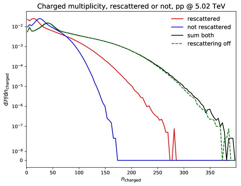
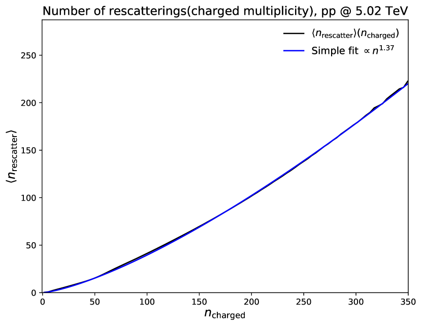
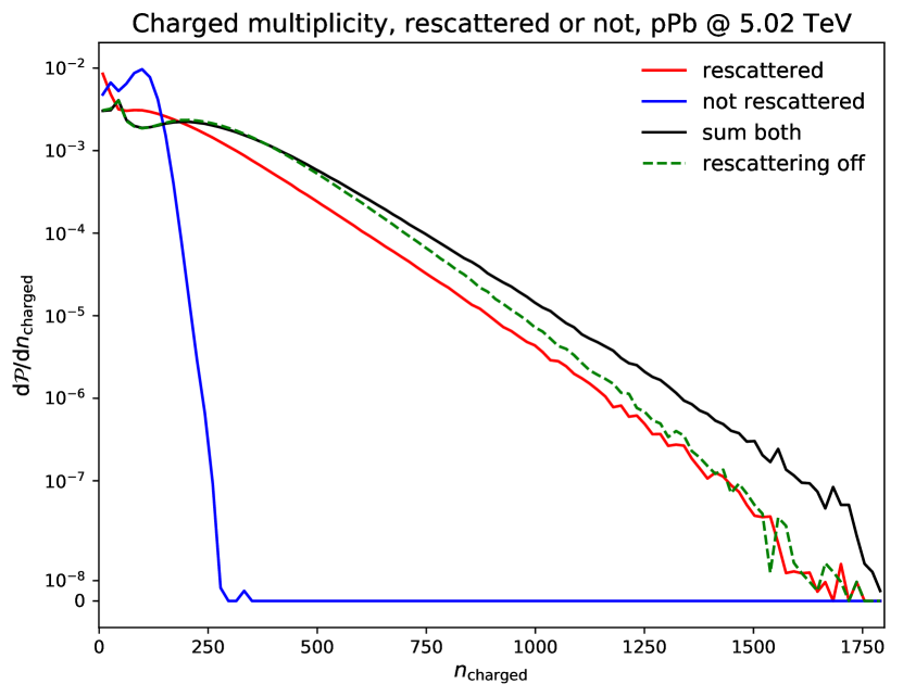
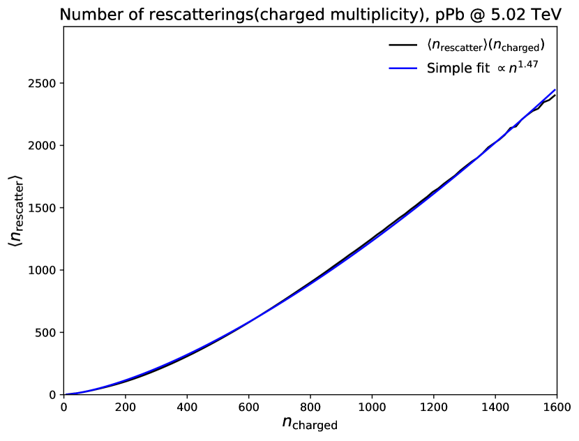
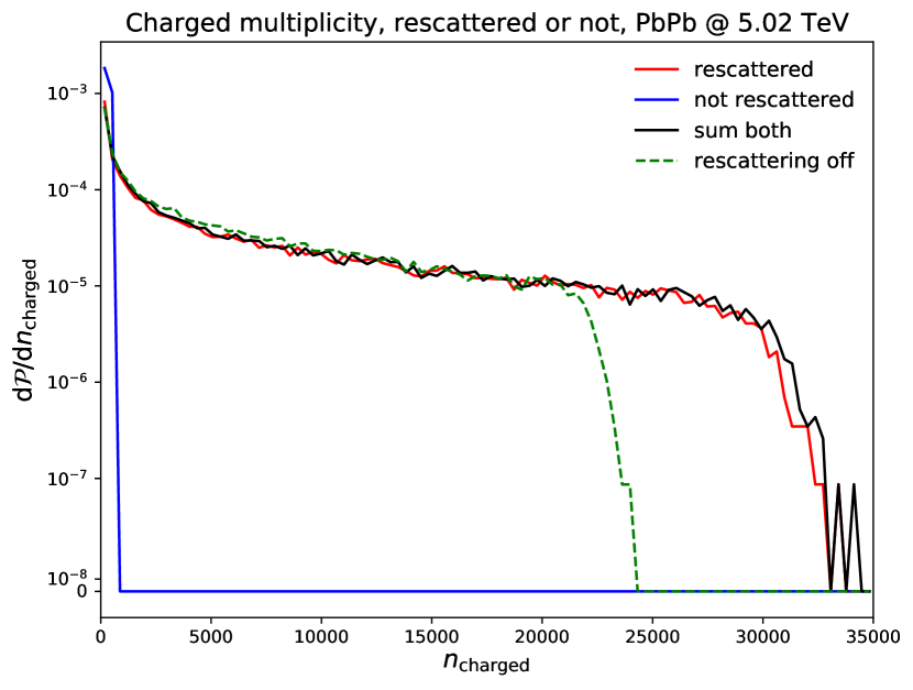
(a)

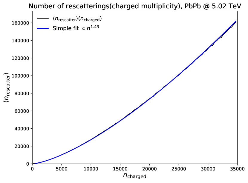
(b)

Figure 1: (a) Probability distributions for the total number of charged hadrons, with and without rescattering, as well as the former number split in those where the final charged hadrons have been affected (directly or indirectly) by rescattering and those where not. (b) Average number of rescatterings as a function of the charged hadron multiplicity, together with a simple fit proportional to $n_{\mathrm{ch}}^{p}$.

Charged multiplicity distributions are shown in Figure 1a, split into hadrons that have or have not been affected by rescattering. Particles with a proper lifetime $\tau_{0}>100$ fm have been considered stable, and multiplicities are reported without any cuts on $\eta$ or $p_{\perp}$. Moving from $\mathrm{p}\mathrm{p}$ to $\mathrm{p}\mathrm{Pb}$ to $\mathrm{PbPb}$ we see how the fraction of particles that do not rescatter drops dramatically. In absolute numbers there still are about as many unrescattered in $\mathrm{p}\mathrm{Pb}$ as in $\mathrm{p}\mathrm{p}$, and about twice as many in $\mathrm{PbPb}$. A likely reason is that many collisions are peripheral, and even when not there are particles produced at the periphery.

The total charged multiplicity is also compared with and without rescattering. As foretold, the $\mathrm{p}\mathrm{p}$ case has there been tuned to show no difference, whereas rescattering enhances the high-multiplicity tail in $\mathrm{p}\mathrm{Pb}$ and $\mathrm{PbPb}$. Rescattering also changes the relative abundances of different particle types. In particular, baryon-antibaryon annihilation depletes the baryon rate, by 7.5 % for $\mathrm{p}\mathrm{p}$, 9.9 % for $\mathrm{p}\mathrm{Pb}$ and 23.4 % for $\mathrm{PbPb}$, compared to the baryon number with a retuned $p_{\perp 0}$. The retuning itself gives in all cases a $\sim$2 % reduction, that should be kept separate in the physics discussion. The observed strange-baryon enhancement [52, 14] thus has to be explained by other mechanisms, such as the rope model [26] or other approaches that give an increased string tension [53].

3.2 Rescattering rates

One of the most basic quantities of interest is the number of rescatterings in an event. The average number of rescatterings as a function of the final charged multiplicity $n_{\mathrm{ch}}$ is shown in Figure 1b. The number of potential interactions at the beginning of rescattering is proportional to $n_{\mathrm{primary}}^{2}$, where the number of primary hadrons $n_{\mathrm{primary}}\simeq n_{\mathrm{ch}}$. The scaling is different in practice however, due to the fact that some particles rescatter several times, while others do not rescatter at all. As a first approximation one might still expect the number of rescatterings to increase as $n_{\mathrm{ch}}^{p}$ for some power $p$. As seen in Figure 1b, this relation appears to hold remarkably well, with $p=1.37$ for $\mathrm{p}\mathrm{p}$, $p=1.47$ for $\mathrm{p}\mathrm{Pb}$, and $p=1.43$ for $\mathrm{PbPb}$. Interestingly, the exponent is highest for the intermediate case $\mathrm{p}\mathrm{Pb}$, but the rescattering activity as such is still highest for $\mathrm{PbPb}$. A possible explanation could be that in $\mathrm{PbPb}$, high multiplicity corresponds to more central events with a larger volume, and thus higher multiplicity does not necessarily mean higher density in this case. We have also studied other $\mathrm{p}\mathrm{A}$ and $\mathrm{A}\mathrm{A}$ cases for a wide variety of sizes of $\mathrm{A}$, including Li, O, Cu and Xe. While there is some $\mathrm{A}$ dependence in the exponent, this variation is less significant than the overall difference between the $\mathrm{p}\mathrm{A}$ and $\mathrm{A}\mathrm{A}$ cases, and in all instances the respective $p$ numbers for $\mathrm{p}\mathrm{Pb}$ and $\mathrm{PbPb}$ provide a reasonable description.

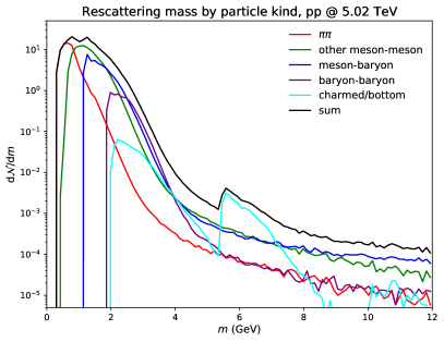
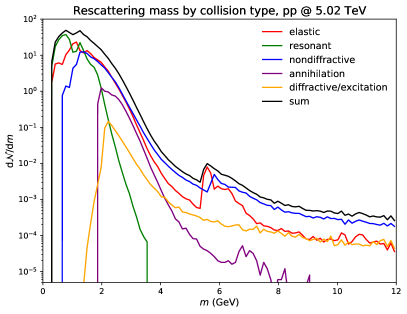
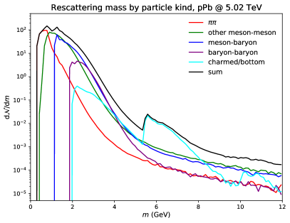
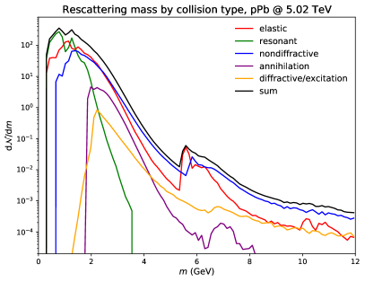
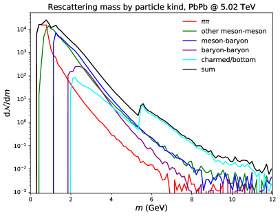
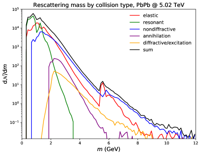
(a)

(b)

Figure 2: Invariant masses for rescatterings, (a) by particle kind and (b) by rescattering process type.

The invariant mass distributions of rescatterings are shown in Figure 2a by incoming particle kind and in Figure 2b by rescattering type. For increasingly large systems the fraction of low-mass rescatterings goes up. A likely reason for this is rescattering causes a greater multiplicity increase in the larger systems, reducing the average energy of each particle. The composition of collision types at a given mass is the same (within errors), as could be expected. Our rescattering model is based on a non-perturbative framework intended to be reasonably accurate up to around $\sim$10 GeV. It would have to be supplemented by perturbative modelling if a significant fraction of the collisions were well above 10 GeV, but clearly that is not the case. As an aside, the bump around 5.5 GeV comes from interactions involving bottom hadrons.

3.3 Transverse momentum spectra

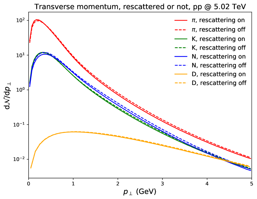
(a)

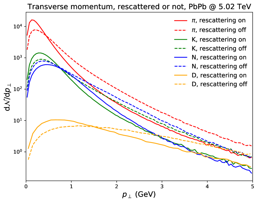
(b)

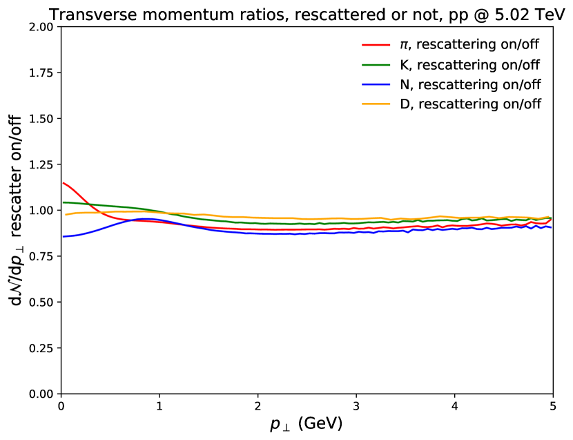
(c)

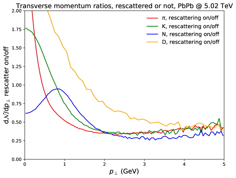
(d)

Figure 3: $p_{\perp}$ spectra for pions, kaons, nucleons and D mesons, for (a) $\mathrm{p}\mathrm{p}$ and (b) $\mathrm{PbPb}$, together with ratios between the spectra with to without rescattering, for (c) $\mathrm{p}\mathrm{p}$ and (d) $\mathrm{PbPb}$.

The $p_{\perp}$ spectra for pions, kaons, nucleons and charm mesons, with and without rescattering, are shown in Figure 3a,b, and the ratios with/without are shown in Figure 3c,d. The effects are qualitatively similar for $\mathrm{p}\mathrm{p}$ and $\mathrm{PbPb}$, but more prominent for the latter case. Pions get pushed to lower $p_{\perp}$, which is consistent with the expectation that lighter particles will lose momentum due to the “pion wind” phenomenon, where lighter particles move faster than heavier and push the latter ones from behind. We remind that all primary hadrons types are produced with the same $p_{\perp}$ distribution in string fragmentation, if the string is stretched parallel with the collision axis. Rapid $\rho$ and $\mathrm{K}^{*}$ decays decrease the average pion $p_{\perp}$, but initially indeed pions have the largest velocities.

The effect is similar for kaons, which unfortunately is inconsistent with measurement [52]. Our studies indicate that a significant contribution to the loss of $\langle p_{\perp}\rangle$ for kaons comes from inelastic interactions, and that the $\langle p_{\perp}\rangle$ increases if all rescatterings are forced to be elastic. We believe this effect can be ameliorated by implementing $3\to 2$ and related processes. For nucleons we note an overall loss in the rescattering scenario, which comes mainly from baryon–antibaryon annihilation, as already mentioned. The $\langle p_{\perp}\rangle$ is shifted upwards by the aforementioned pion wind phenomenon.

$\mathrm{D}$ mesons are enhanced at low $p_{\perp}$, all the way down to threshold. At first glance this appears inconsistent with the pion wind phenomenon, since $\mathrm{D}$ mesons are heavy. One key difference is that charm quarks are not produced in string fragmentation, but only in perturbative processes. Therefore $\mathrm{D}$ mesons start out at higher $p_{\perp}$ values than ordinary hadrons, and can lose momentum through rescattering. Nevertheless, the overall shift is still somewhat towards higher momenta if only elastic rescatterings are permitted, as for kaons.

Overall we see a rather significant effect on $p_{\perp}$ spectra, and this is to be kept in mind for other distributions. Especially for pions, where the choice of a lower $p_{\perp}$ cut in experimental studies strongly affects the (pseudo)rapidity spectrum deformation by rescattering, among others.

3.4 Spacetime picture of rescattering

In this section we study the spacetime distributions of rescatterings. Specifically, we consider the transverse production distance, $r_{\perp}^{2}=x^{2}+y^{2}$, and longitudinal invariant time, $\tau_{L}^{2}=t^{2}-z^{2}$. The two Lorentz-contracted “pancake” nuclei are set to collide at $t=z=0$, with the center of collision at $x=y=0$, but with sub-collisions spread all over the $(x,y)$ overlap region. Thus the squared invariant time $\tau^{2}=t^{2}-x^{2}-y^{2}-z^{2}=\tau_{L}^{2}-r_{\perp}^{2}$ tends to have a large tail out to large negative values, so it is not a suitable measure for heavy-ion collisions. The $r_{\perp}$ and $\tau_{L}$ distributions are shown in Figure 4, separately for particles involved or not in rescattering. For the latter it is the location of the last rescattering that counts. Particle decays are included for particles with proper lifetimes $\tau_{0}<100$ fm, so that a “final” pion could be bookkept at the decay vertex of for instance a $\rho$.

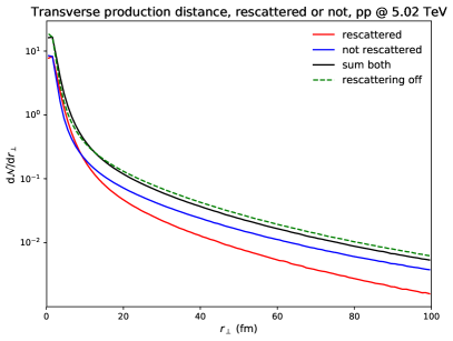
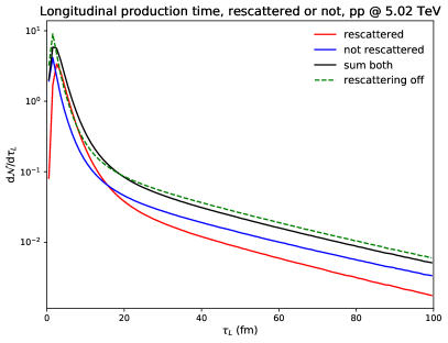
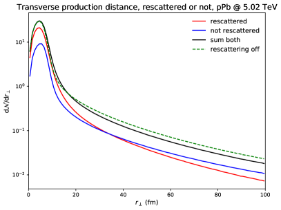
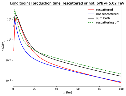
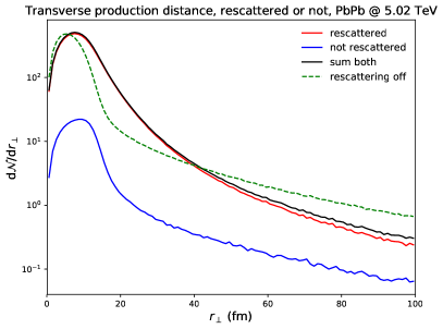
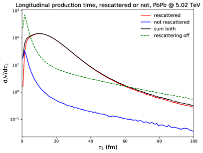
(a)

(b)

Figure 4: (a) $r_{\perp}$ and (b) $\tau_{L}$ spectra. Note that rescattered also refers to hadrons produced in decays of rescattered particles, even though they themselves were not directly involved in rescattering.

The overall observation is that rescattering reduces particle production at very early and at late times, as is especially clear in the $\tau_{L}$ distribution for $\mathrm{PbPb}$. Particles produced at early times are more likely to participate in rescattering and get assigned new $\tau_{L}$ values on the way out. With this in mind, it may seem paradoxical that the $r_{\perp}$ distributions are comparably broad for rescattered and unrescattered particles. Hadrons produced in the periphery of the collision are more likely to evade rescattering than central ones, however, so this introduces a compensating bias towards larger $r_{\perp}$ for the unrescattered. In this respect the $\tau_{L}$ distribution more follows the expected pattern, with the unrescattered particles having comparable average values in all three collision scenarios, whereas the rescattered ones are shifted further out. Maybe somewhat unexpectedly, particle production at late times and large $r_{\perp}$ is also reduced with rescattering on. Our studies indicate that there is some rescattering activity at late times ($\gtrsim 50$ fm), but the number of rescatterings here is roughly a factor of three smaller than the number of decays. Now, since rescattering produces more particles early, it tends to reduce the average particle mass, which increases the number of stable particles produced early and reduces the number of decaying ones in the $50-100$ fm range. Furthermore, unstable particles often have lower $p_{\perp}$ and hence smaller Lorentz factors, leading them to decay at lower $r_{\perp}$ values.

While the exact time of a rescattering cannot be measured directly, phenomena such as resonance suppression can give an indication of the duration of the hadronic phase [54, 55]. Experimentally, a suppression of the $\mathrm{K}^{*}/\mathrm{K}$ yield ratio at higher multiplicities has been observed, but not of the $\phi/\mathrm{K}$ yield ratio. The interpretation of this observation is as follows: after the $\mathrm{K}^{*}$ decays, the outgoing $\pi$ and $\mathrm{K}$ are likely to participate in rescattering because of their large cross sections, which disturbs their correlation and suppresses the original $\mathrm{K}^{*}$ signal. The fact that the $\phi$ signal is not suppressed in this way indicates that they tend to decay only after most rescattering has taken place. With the $\mathrm{K}^{*}$ and $\phi$ lifetimes being 3.9 fm and 46.3 fm respectively, this places bounds on the duration of the rescattering phase. These bounds seem to be consistent with the spacetime distributions shown in Figure 4.

With the full event history provided by Pythia, it is possible to study the actual number of $\mathrm{K}^{*}$ and $\phi$ that were produced, and to trace what happens to their decay products. A naïve way to approach resonance suppression is to define a $\mathrm{K}^{*}$ or $\phi$ meson as detectable if it decayed and no decay product participated in rescattering. When defining the $\mathrm{K}^{*}$ multiplicity in this way, we found that rescattering actually increases the $\mathrm{K}^{*}/\mathrm{K}$ ratio for larger charged multiplicities. This increase is not observable, however, since it mainly comes from $\mathrm{K}\pi\to\mathrm{K}^{*}\to\mathrm{K}\pi$. That is, some of the combinatorial background gets to be reclassified as $\mathrm{K}^{*}$, without any change of the overall $\mathrm{K}\pi$ mass spectrum. To find the more subtle effects of nontrivial processes requires a detailed fitting of the $\mathrm{K}\pi$ mass spectrum. This is outside the scope of this article, but would be interesting to study in the future. Nevertheless, the change in the $\phi/\mathrm{K}$ ratio is much smaller, suggesting that qualitatively, longer-lived resonances are indeed less affected by rescattering.

3.5 Centrality dependent observables

In heavy ion experiments, observables are most often characterized according to collision centrality. The characterization is a sensible one, also for checking the effects of hadronic rescatterings, as this will be the largest in the most central collisions. While experiments employ a centrality definition depending on particle production in the forward or central regions of the experiments, we will in the following sections use the definition adhering to impact parameter. As such, the centrality of a single collision is defined as

$$c=\frac{1}{\sigma_{\mathrm{inel}}}\int_{0}^{b}\mathrm{d}b^{\prime}\frac{\mathrm{d}\sigma_{\mathrm{inel}}}{\mathrm{d}b^{\prime}}.$$ (4)

We note, however, that the results presented for nucleus-nucleus collisions can be transferred directly to experimental centrality measures, as the Angantyr model provides a good description of eg. forward energy, which correlates directly with the theoretical impact parameter.

3.5.1 Particle yields and ratios

In the following we present the effect on identified particle yields in $|y|<4$ (to avoid the beam region) in $\mathrm{XeXe}$ collisions at $\sqrt{s_{\mathrm{N}\mathrm{N}}}=5.44$ TeV and $\mathrm{PbPb}$ collisions at $\sqrt{s_{\mathrm{N}\mathrm{N}}}=2.76$ TeV. Starting with light flavour mesons and baryons, we show the average multiplicity of (a) pions ($\pi^{\pm}$) and (b) protons ($\mathrm{p},\overline{\mathrm{p}}$) per event in Figure 5 and respectively.

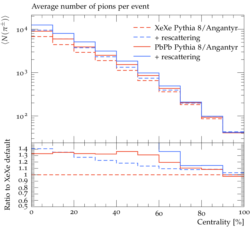
(a)

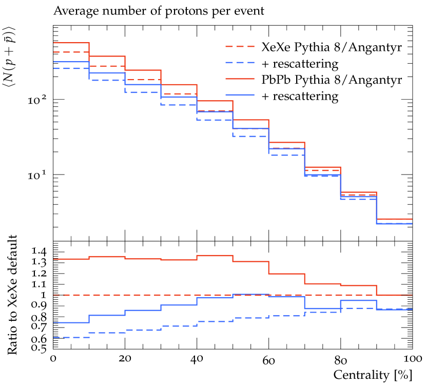
(b)

Figure 5: Average per-event yields of (a) pions $(\pi^{\pm})$ and (b) protons ($\mathrm{p},\overline{\mathrm{p}}$) in $\mathrm{PbPb}$ and $\mathrm{XeXe}$ collisions at $\sqrt{s_{\mathrm{N}\mathrm{N}}}=$ 2.74 and 5.44 TeV respectively, as function of collision centrality.

While the effect for pions is negligible in peripheral collisions, it grows to about 40% in central collisions. The effect on protons is also largest in central collisions, while in peripheral collisions it is still at a 10% level. This is particularly interesting in the context of recent years’ introduction of microscopic models to explain the increase of strange baryon yields with increasing multiplicity, which overestimate the amount of protons [56].

In Figure 6 we move to strange mesons and baryons, with the total kaon ($\mathrm{K}^{\pm}$ and $\mathrm{K}^{0}_{\mathrm{L,S}}$) and $\Lambda$ multiplicity, (a) and (b) respectively. While there is a large effect on the direct yields of both species, it is almost identical to the change in $\pi^{\pm}$ in Figure 5a, leaving the $\mathrm{K}/\pi$ and $\Lambda/\pi$ ratios unchanged.

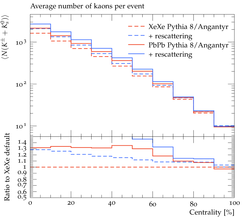
(a)

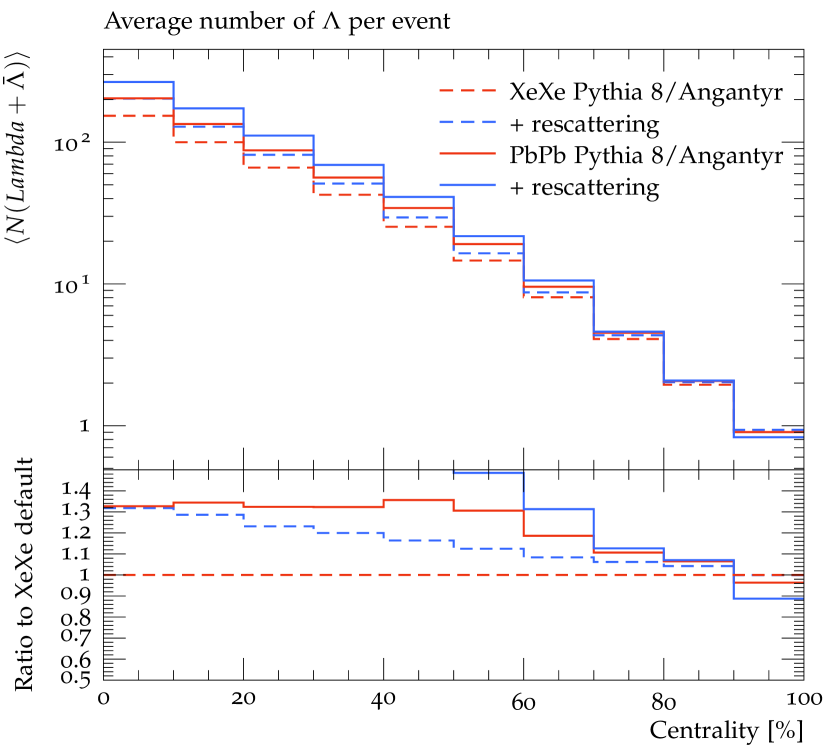
(b)

Figure 6: Average per-event yields of (a) kaons $(\mathrm{K}^{\pm},\mathrm{K}^{0}_{\mathrm{L,S}})$ and (b) $\Lambda$ ($\Lambda,\overline{\Lambda}$) in $\mathrm{PbPb}$ and $\mathrm{XeXe}$ collisions at $\sqrt{s_{\mathrm{N}\mathrm{N}}}=$ 2.74 and 5.44 TeV respectively, as function of collision centrality.

We finish the investigation of the light-flavour sector by showing the total $\phi$ and $\Omega^{-}$ multiplicities in Figure 7a and b respectively. The $\phi$ multiplicity decreases by about 20% in central events and is constant within the statistical errors in peripheral. The $\Omega$ multiplicity is decreased roughly the same amount. The decrease here, however, is rather constant in centrality in $\mathrm{XeXe}$ but increases for central events in $\mathrm{PbPb}$.

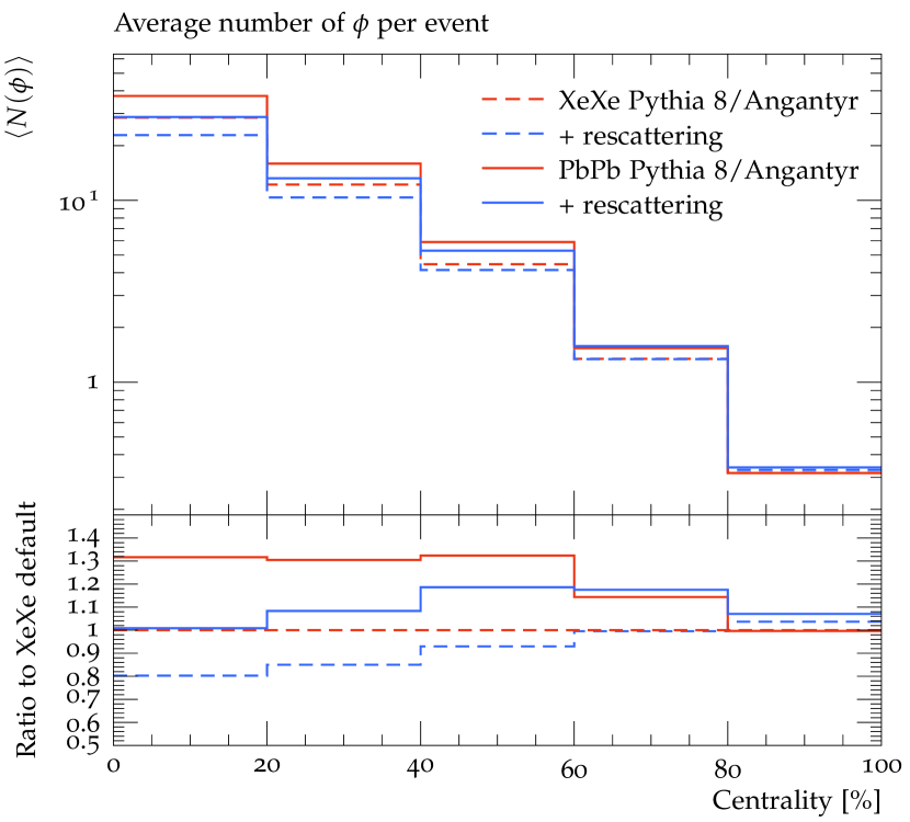
(a)

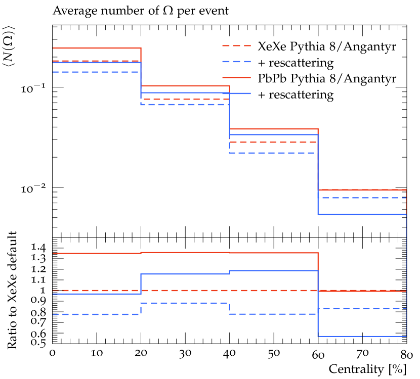
(b)

Figure 7: Average per-event yields of (a) $\phi$ and (b) $\Omega^{-}$ in $\mathrm{PbPb}$ and $\mathrm{XeXe}$ collisions at $\sqrt{s_{\mathrm{N}\mathrm{N}}}=$ 2.74 and 5.44 TeV respectively, as function of collision centrality.

Notably (and as opposed to eg. UrQMD), the rescattering framework implemented in Pythia, includes cross sections for heavy flavour mesons and baryons. In Figure 8 we show the effect on (a) $\mathrm{J}/\psi$ and (b) $\mathrm{D}$ mesons ($\mathrm{D}^{\pm}$ and $\mathrm{D}^{0}$). Starting with the $\mathrm{J}/\psi$ we see a significant effect in both collision systems in central events, less so in peripheral. While the initial $\mathrm{J}/\psi$ yield is roughly 10% larger in $\mathrm{PbPb}$ than in $\mathrm{XeXe}$, the final value after rescattering saturates at a value at roughly 60% of the initial $\mathrm{XeXe}$ value, independent of the two collision systems. Whether or not this is consistent with the measured nuclear modification factor [57] in peripheral collisions (clearly not in central collisions, where an additional source of $\mathrm{J}/\psi$ production would be required) is left for future detailed comparisons to data.

In Pythia (rescattering or not) there is no mechanism for charm quarks to vanish from the event at early times. The constituents of the $\mathrm{J}/\psi$ would therefore have to end up in other charmed hadrons. In Figure 8b we show the $\mathrm{D}$ meson yield, demonstrating that this is more than two orders of magnitude above the $\mathrm{J}/\psi$ one. It is then consistent to assume that the missing charm quarks can recombine into open charm without having observable consequences. Indeed there is no significant effect on the $\mathrm{D}$ meson yield from rescattering.

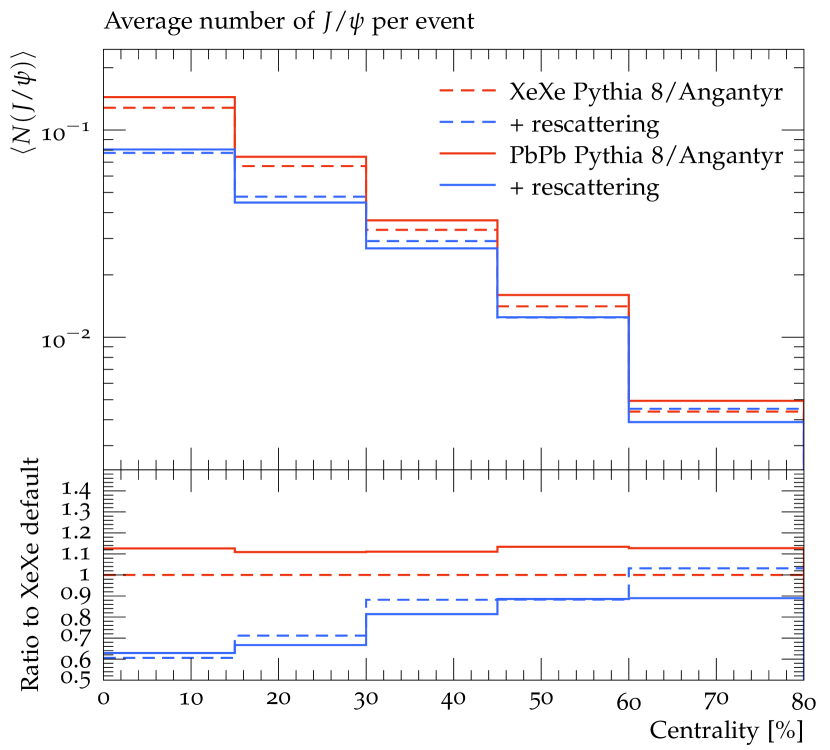
(a)

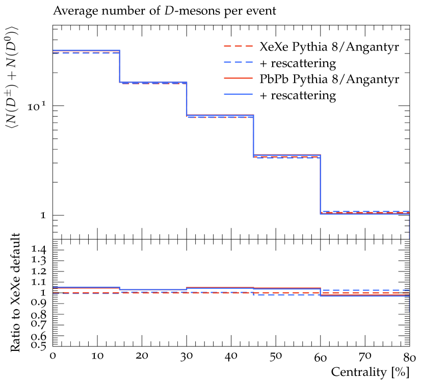
(b)

Figure 8: Average per-event yields of (a) $\mathrm{J}/\psi$ and (b) $\mathrm{D}$ mesons in $\mathrm{PbPb}$ and $\mathrm{XeXe}$ collisions at $\sqrt{s_{\mathrm{N}\mathrm{N}}}=$ 2.74 and 5.44 TeV respectively, as function of collision centrality.

3.5.2 Elliptic flow

One of the most common ways to characterize heavy ion collisions is by the measurement of flow coefficients ($v_{n}$’s), defined as the coefficients of a Fourier expansion of the single particle azimuthal yield, with respect to the event plane $\Psi_{n}$ [58, 59]:

$$E\frac{\mathrm{d}^{3}N}{\mathrm{d}^{3}p}=\frac{1}{2\pi}\,\frac{\mathrm{d}^{2}N}{p_{\perp}\mathrm{d}p_{\perp}\mathrm{d}y}\left(1+2\sum_{n=1}^{\infty}v_{n}\cos(n(\varphi-\Psi_{n}))\right).$$ (5)

The azimuthal angle is denoted $\varphi$, and $E$, $p_{\perp}$ and $y$ are the particle energy, transverse momentum and rapidity respectively. In experiments it is not possible to utilize this definition directly, as the event plane is unknown. Therefore one must resort to other methods. For the purpose of testing if a model behaves as expected, it is on the other hand preferable to measure how much or little particles will correlate with the true event plane (when we show comparisons to experimentally obtained values in Section 4.2, we will use the experimental definitions). In the following, we will therefore use an event plane obtained from the initial state model, defined as

$$\Psi_{n}=\frac{1}{n}\arctan\left(\frac{\langle r^{2}\sin(n\varphi)\rangle}{\langle r^{2}\cos(n\varphi)\rangle}\right)+\frac{\pi}{n},$$ (6)

for all initial state nucleons participating in collisions contributing to the final state multiplicity (inelastic, non-diffractive sub-collisions). The origin is shifted to the center of the sampled distribution of nucleons, and $r$ and $\varphi$ are the usual polar coordinates. Flow coefficients can then simply be calculated as

$$v_{n}=\langle\cos(n(\varphi-\Psi_{n}))\rangle.$$ (7)

As in the previous section we consider all particles in $|y|<4$ and without any lower cut on transverse momentum.

In Figure 9 we show (a) $v_{2}$ and (b) $v_{3}$ as functions of collision centrality for charged particles for $\mathrm{XeXe}$ collisions at $\sqrt{s_{\mathrm{N}\mathrm{N}}}=5.44$ TeV and $\mathrm{PbPb}$ collisions at $\sqrt{s_{\mathrm{N}\mathrm{N}}}=2.74$ TeV both with and without rescattering. It is seen that $v_{2}$ receives a sizeable contribution from rescattering. The contribution is larger for $\mathrm{PbPb}$ than for $\mathrm{XeXe}$, which is not surprising, given the larger density. The $v_{2}$ arises because particles are pushed by rescatterings along the density gradient, which is larger along the event plane. Note that the curve without rescattering is zero, as the definition of $v_{n}$ from eq. (7) ensures that no non-flow contributions enter the results.

For $v_{3}$ (Figure 9b) there is not much difference between $\mathrm{PbPb}$ and $\mathrm{XeXe}$. Since $v_{3}$ is mainly generated by initial state shape fluctuations, this is a reasonable result.

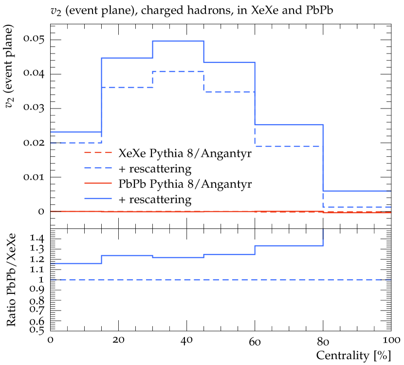
(a)

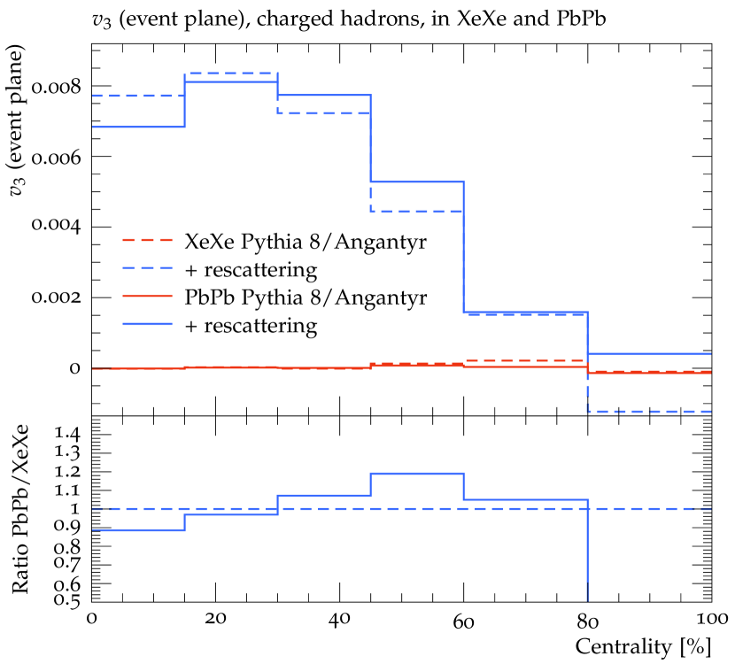
(b)

Figure 9: Flow coefficients (a) $v_{2}$ and (b) $v_{3}$ in $\mathrm{PbPb}$ and $\mathrm{XeXe}$ collisions at $\sqrt{s_{\mathrm{N}\mathrm{N}}}=$ 2.74 and 5.44 TeV respectively. Results shown with and without rescattering, and are calculated with respect to the event plane such that the sample without rescattering is zero by construction.

Since different hadron species have different cross sections, hadronic rescattering will yield different flow coefficients for different hadron species. As an example, since the $\mathrm{p}\mathrm{p}(\overline{\mathrm{p}}\mathrm{p})$ cross section is larger than the average hadron-hadron cross section (which is dominated mainly by pions), $v_{2}$ for protons will be higher. We note (without showing) that hadronic rescattering gives $v_{2}(\mathrm{p})>v_{2}(\pi)>v_{2}(\mathrm{K})\approx v_{2}(\Lambda)>v_{2}(\Omega)>v_{2}(\phi)$, with the latter reaching its maximum for $v_{2}$ about an order of magnitude less than for protons.

For heavy flavours, the results require more explanation, due to the differing production mechanisms. In Pythia, $\mathrm{D}$ mesons are produced in string fragmentation, requiring that one of the quark ends is a charm quark. The $\mathrm{J}/\psi$, on the other hand, is predominantly produced early, either by direct onium production via colour-singlet and colour-octet mechanisms, or by an early “collapse” of a small $\mathrm{c}\overline{\mathrm{c}}$ string to a $\mathrm{J}/\psi$. Onia are therefore excellent candidates for hadrons mainly affected by hadronic rescattering, and not any effects of strings interacting with each other before hadronization.

In Figure 10, we show $v_{2}$ for (a) $\mathrm{D}$ mesons and (b) $\mathrm{J}/\psi$. Starting with $\mathrm{D}$ mesons we see an appreciable $v_{2}$, numerically not too far from $\mathrm{PbPb}$ data [60]. A clear difference is observed between $\mathrm{XeXe}$ and $\mathrm{PbPb}$. In the figure, statistical error bars are shown, as they are not negligible due long processing times for heavy flavour hadrons. For the $\mathrm{J}/\psi$, shown in Figure 10b, $v_{2}$ for $\mathrm{PbPb}$ and $\mathrm{XeXe}$ are compatible within the statistical error. More importantly, the result is also compatible with experimental data [61]. Together with the result from Figure 8a, which suggests a sizeable nuclear modification to the $\mathrm{J}/\psi$ yield from rescattering, a detailed comparison with available experimental data should be performed. It should be noted that the treatment of charm in the Pythia hadronic rescattering model follows the additive quark model, as introduced earlier. Thus, no distinction is made between $\mathrm{J}/\psi$ and other $\mathrm{c}\overline{\mathrm{c}}$ states. A foreseen improvement of this treatment would be to consider differences with input taken eg. from lattice calculations.

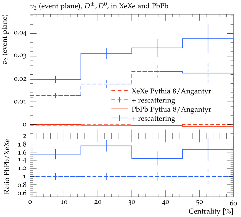
(a)

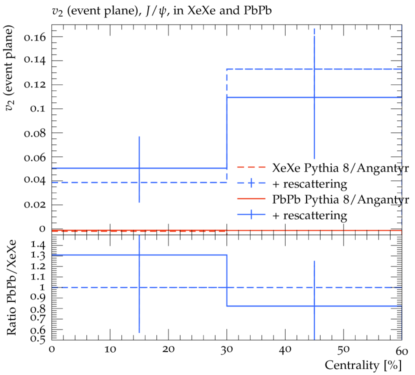
(b)

Figure 10: The $v_{2}$ flow coefficient for (a) $\mathrm{D}$ mesons ($\mathrm{D}^{\pm},\mathrm{D}^{0}$) and (b) $\mathrm{J}/\psi$ as a function of centrality in $\mathrm{PbPb}$ and $\mathrm{XeXe}$ collisions at $\sqrt{s_{\mathrm{N}\mathrm{N}}}=$ 2.74 and 5.44 TeV respectively. Error bars are statistical errors. Results shown with and without rescattering, and are calculated with respect to the event plane such that the sample without rescattering is zero by construction.

4 Comparison with data

In this section we go beyond the model performance plots shown in the previous section, and compare to relevant experimental data for $\mathrm{XeXe}$ and $\mathrm{PbPb}$, in cases where Rivet [62] implementations of the experimental analysis procedure are available (though not in all cases validated by experiments). We focus on observables where the rescattering effects are large, and in some cases surprising.

In all cases centrality is defined according to eq. (4), as it reduces computation time, and the difference between centrality defined by impact parameter and forward energy flow is not large in $\mathrm{A}\mathrm{A}$ collisions.

4.1 Charged multiplicity

In section 3.1 we described how the current lack of $3\to 2$ processes in the rescattering framework increases the total multiplicities. In Figure 11 Angantyr with and without rescattering is compared to experimental data [63, 64].

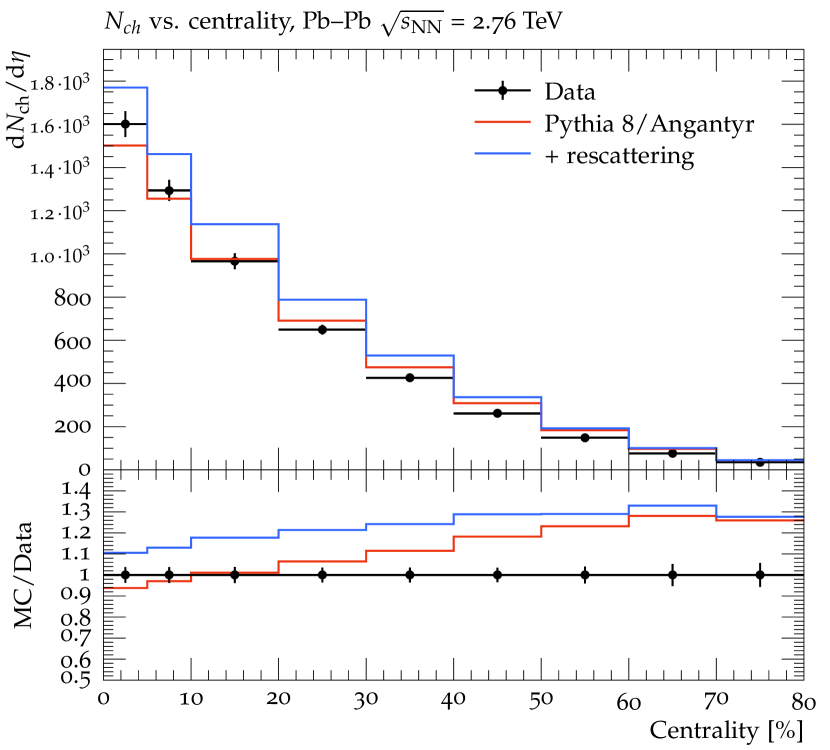
(a)

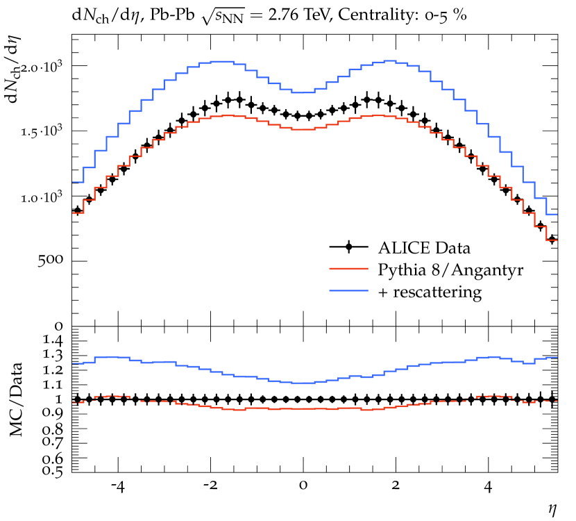
(b)

Figure 11: Charged multiplicities in $\mathrm{PbPb}$ collisions $\sqrt{s_{\mathrm{N}\mathrm{N}}}=2.76$ TeV. At mid-rapidity as (a) function of centrality, and (b) differential in $\eta$ in centrality 0-5%. Data from ALICE [63, 64].

In Figure 11a, $\mathrm{dN}_{ch}/\mathrm{d}\eta|_{\eta=0}$ is shown as function of centrality. It is clear that the shift in multiplicity, caused by rescattering, is centrality dependent, with a larger effect seen in more central events. For centrality 0-5%, the agreement with data shifts from approximately 8% below data to 10% above. It is instructive to show the differential distributions as well, and in Figure 11b, the $\eta$-distribution out to $\pm 5$ is shown. It is seen that the shift is slightly larger at the edges of the plateau. This effect is most pronounced in the centrality bin shown here, and decreases for more peripheral events.

To further explore the change in charged multiplicity distributions, we show comparisons to invariant $p_{\perp}$ distributions in the same collision system, measured down to $p_{\perp}=0.15$ GeV in $|\eta|<0.8$ [65] in Figure 12, with 0-20% centrality shown in Figure 12a, and 40-60% in Figure 12b. It is seen that particles at intermediate $p_{\perp}\approx 1-6$ GeV are pushed down to very low $p_{\perp}$ (pion wind) in rescatterings which, due to the lack of $3\to 2$ processes, will generate more final state particles overall.

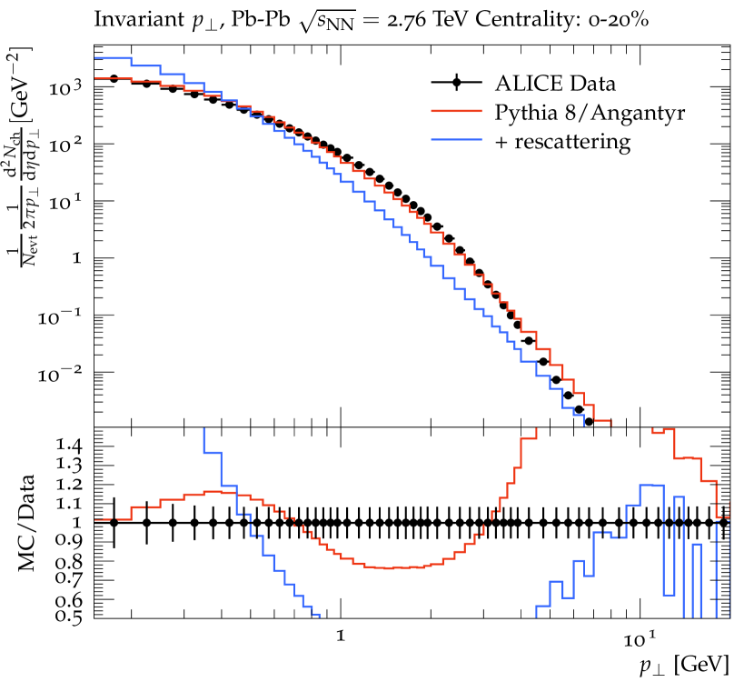
(a)

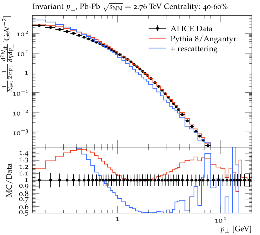
(b)

Figure 12: Invariant $p_{\perp}$ spectra of charged particles in $\mathrm{PbPb}$ collisions $\sqrt{s_{\mathrm{N}\mathrm{N}}}=2.76$ TeV, in $|\eta|<0.8$. Shown for two different centrality intervals (a) 0-20% and (b) 40-60%. Data from ALICE [65].

From this investigation of effects on basic single-particle observables from adding rescattering, it is clear that agreement with data is decreased. Since hadronic rescattering in heavy ion collisions is physics effects which must be taken into account, this clearly points to the need of further model improvement. Beyond re-tuning and adding $3\to 2$ processes, the addition of string-string interactions before hadronic rescattering will change the overall soft kinematics. This is an important next step, which will be taken in a forthcoming publication.

4.2 Flow coefficients

As indicated in section 3.5, rescattering has a non-trivial effect on flow observables, a staple measurement in heavy ion experiments. Anisotropic flow is generally understood as a clear indication of QGP formation, as it is well described by hydrodynamic response to the anisotropy of the initial geometry [66].

The main difference between most previous investigations and this paper, of the effect of rescattering on flow, is the early onset of the hadronic phase. Recall that with a hadronization time of $\langle\tau^{2}\rangle\approx 2$ fm², the initial hadronic state from string hadronization is much denser.

In this section we will compare to experimental data from $\mathrm{XeXe}$ and $\mathrm{PbPb}$ collisions obtained by the ALICE experiment [13]. When doing so, it is important to use the same definitions of flow coefficients as used by the experiment. Since the event plane is not measurable by experiment, equations (5) and (7) cannot be applied directly. Instead the flow coefficients are calculated using two- and multi-particle azimuthal correlations using the so-called generic framework [67], implemented in the Rivet framework [68], including the use of sub-events [69].

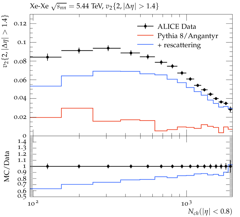
(a)

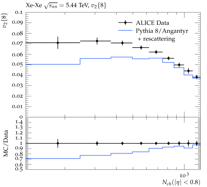
(b)

Figure 13: Elliptic flow in $\mathrm{XeXe}$ collisions at $\sqrt{s_{\mathrm{N}\mathrm{N}}}=5.44$ TeV. (a) $v_{2}\{2\}$ with $|\Delta\eta|>1.4$ and (b) $v_{2}\{8\}$. The $v_{2}$ calculated with 4- and 6-particle correlations show a similar trend, but are not shown in the figure. Data from ALICE [13].

In figure 13 we show elliptic flow $v_{2}$ in $\mathrm{XeXe}$ collisions at $\sqrt{s_{\mathrm{N}\mathrm{N}}}=5.44$ TeV calculated with (a) two-particle correlations and $|\Delta\eta|>1.4$, as well as (b) $v_{2}\{8\}$. In the former case we compare also to the no-rescattering option, which gives a measure of contributions from non-flow mechanisms such as (mini)jets and particle decays. In both cases the data is reproduced with good (within 10%) accuracy for very high multiplicities, but the calculation is up to 30-40% below data for more peripheral events. It is particularly interesting to note that even in the case of using an 8-particle correlator, the calculation shows the same agreement as only two particles with a gap in $\eta$ between them. This rules out the possibility that additional flow enters purely from a local increase in two-particle correlations. This should also already be clear from the treatment in section 3.5, where it was clearly shown that the added $v_{2}$ by rescattering is in the correct direction with respect to the theoretical event plane.

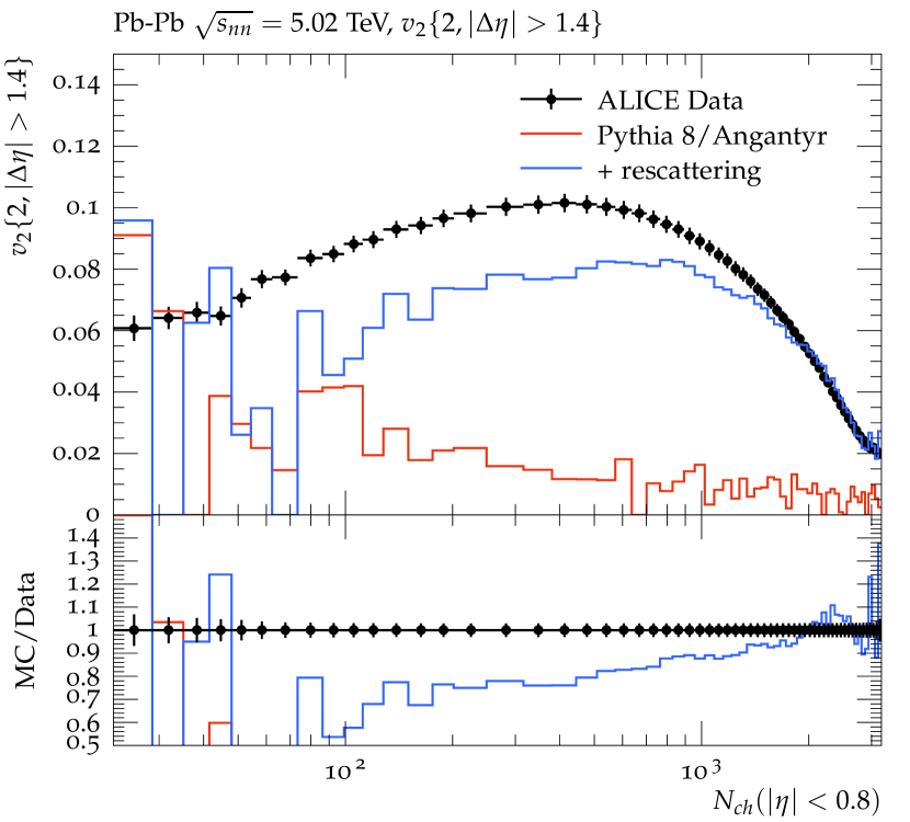
(a)

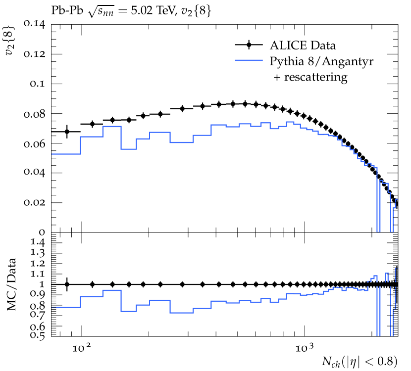
(b)

Figure 14: Elliptic flow in $\mathrm{PbPb}$ collisions at $\sqrt{s_{\mathrm{N}\mathrm{N}}}=5.02$ TeV. (a) $v_{2}\{2\}$ with $|\Delta\eta|>1.4$ and (b) $v_{2}\{8\}$. The $v_{2}$ calculated with 4- and 6-particle correlations show a similar trend, but are not shown in the figure. Data from ALICE [13].

In figure 14 we show the same observables, $v_{2}\{2,~{}|\Delta\eta|>1.4\}$ and $v_{2}\{8\}$ for $\mathrm{PbPb}$ collisions at $\sqrt{s_{\mathrm{N}\mathrm{N}}}=5.02$ TeV. While the same overall picture is repeated, it is worth noticing that the agreement at high multiplicities is slightly better. As it was also observed in section 3.5, the effect of rescattering is in general larger in $\mathrm{PbPb}$ than in $\mathrm{XeXe}$, due to the larger multiplicity of primaries.

We want here to emphasize that, while hadronic rescattering can obviously not describe data for elliptic flow completely, the results here suggest that hadronic rescattering with early hadronization has a larger effect than previously thought. This is particularly interesting seen in the connection with recent results, that interactions between strings before hadronization in the string shoving model [25] will also give a sizeable contribution to flow coefficients in heavy ion collisions, without fully describing data. The combination of the two frameworks, to test whether the combined effect is compatible with data, will be a topic for a future paper. It should be mentioned that the contributions from different models, acting one after the other, does not add linearly [70, 30].

4.3 Jet modifications from rescattering

As shown, both in Figure 3 and Figure 12, hadronic rescattering has a significant effect on high-$p_{\perp}$ particle production. Studies of how the behaviour of hard particles changes from $\mathrm{p}\mathrm{p}$ to $\mathrm{A}\mathrm{A}$ collisions are usually aiming at characterising the interactions between initiator partons and the QGP. The observed phenomena are referred to as “jet quenching”, and phenomenological studies usually ignore the presence of a hadronic phase. For a notable exception see ref. [71] for a recent exploratory study using SMASH, as well as references therein.

In this final results section, we do not wish to go into a full study on the effect of rescattering on jet observables, but rather point to an interesting result which will be pursued further in a future study, as well as warn potential users of the Pythia rescattering implementation of a few pitfalls.

One of the early key observations of jet quenching effects was the disappearance of back-to-back high-$p_{\perp}$ hadron correlations in central $\mathrm{AuAu}$ collisions at RHIC [72]. Similar studies have since also been performed at the ALICE experiment, and we compare here to data from a study of azimuthal modifications in $\mathrm{PbPb}$ collisions at $\sqrt{s_{\mathrm{NN}}}=2.76$ TeV [73]. In this study, trigger particles of $8$ GeV $<p_{\perp,\mathrm{trig}}<15$ GeV are correlated in $\varphi$ with associated particles of $4$ GeV $<p_{\perp,\mathrm{assoc}}<p_{\perp,\mathrm{trig}}$. The $\mathrm{PbPb}/\mathrm{pp}$ ratio of per-trigger yields is denoted $I_{\mathrm{A}\mathrm{A}}$, and it was noted in the study by ALICE that the $\mathrm{PbPb}$ per-trigger yield is suppressed to about 60% of $\mathrm{p}\mathrm{p}$ on the away side ($\Delta\varphi$ of $\pi\pm 0.7$) and enhanced by about 20% on the near side ($\Delta\varphi$ of $\pm 0.7$). In Figure 15, $I_{\mathrm{A}\mathrm{A}}$ in $0-5$% centrality for $\mathrm{PbPb}$ collisions is shown on (a) the near-side and (b) the away side, compared to ALICE data [73].

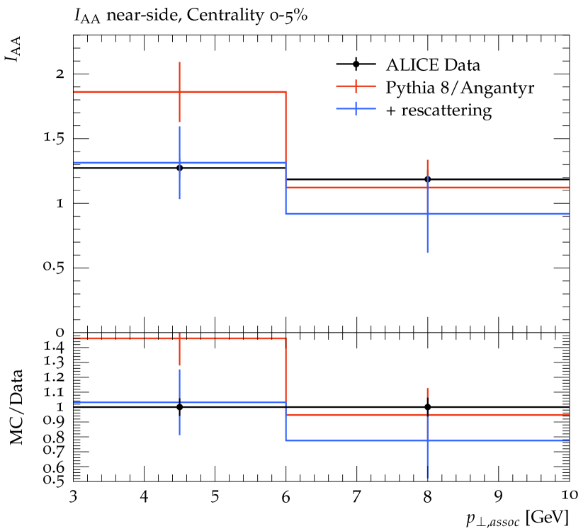
(a)

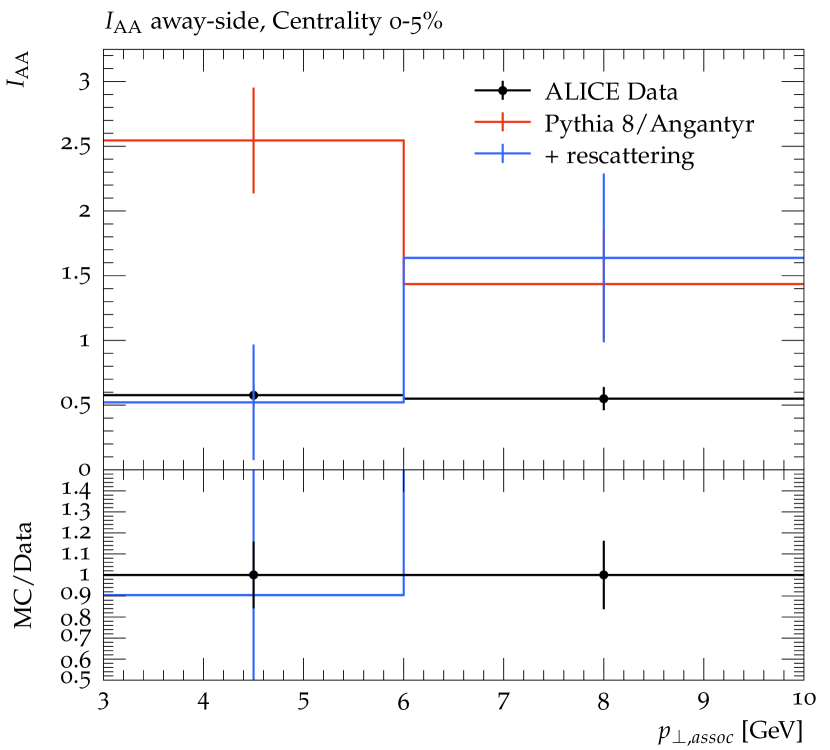
(b)

Figure 15: Modification of high-$p_{\perp}$ azimuthal correlations, $I_{\mathrm{A}\mathrm{A}}$, in $\mathrm{PbPb}$ collisions at $\sqrt{s_{\mathrm{N}\mathrm{N}}}=2.76$ TeV on (a) the near side ($\Delta\varphi$ of $\pm 0.7$) and (b) the away side ($\Delta\varphi$ of $\pi\pm 0.7$), both in the $0-5$% centrality bin. Error bars are statistical errors. Data from ALICE [73].

It is seen that, by default, Pythia/Angantyr overestimates the away-side $I_{\mathrm{A}\mathrm{A}}$ in the whole $p_{\perp,\mathrm{assoc}}$ range, while the near-side is overestimated at low $p_{\perp}<6$ GeV. Adding rescattering brings the simulation on par with data in all cases but the high-$p_{\perp}$ part of the away-side $I_{\mathrm{A}\mathrm{A}}$. No significant effect from rescattering was observed in peripheral events.

At first sight, this seems like a very significant result, but we wish to provide the reader with a word of caution. We remind that the current lack of $n\to 2$ processes and retuning causes a drastic shift in $p_{\perp}$ spectra as previously shown, incompatible with data. The depletion seen from rescattering is exactly in the region where $I_{\mathrm{A}\mathrm{A}}$ is now well reproduced. It can therefore very well be that the effect seen is mainly a token of current shortcomings. This is of course not a statement that hadronic rescattering has no impact on jet-quenching observables, but it goes to show that a potential user cannot run Pythia to explain this or similar observables without a deeper analysis.

Finally a technical remark. Running Pythia/Angantyr with rescattering to reproduce an observable requiring a high-$p_{\perp}$ trigger particle will require very long run times. The figures in this section are generated by first requiring that a parton–parton interaction with $\hat{p}_{\perp}>5$ GeV takes place at all, and secondly a veto is put in place ensuring that the time-consuming rescattering process is not performed if there are no trigger particles with the required $p_{\perp}$ present in the considered acceptance.

5 Summary and outlook

The Pythia rescattering framework was first introduced in [31], which focused on validating it in the context of $\mathrm{p}\mathrm{p}$ collisions. In this paper, the main focus has been physics studies in $\mathrm{p}\mathrm{Pb}$ and $\mathrm{PbPb}$ collisions.

Before going into finer details, it is worth to consider how rescattering changes the bulk properties of events. Notably it increases the charged multiplicity by about 20 % in $\mathrm{PbPb}$ events. One key reason is that we have implemented $2\to n,n>2$ processes but not $n\to 2$. For a system in thermal equilibrium the two kinds should balance each other. In the modelling of $\mathrm{PbPb}$ collisions, however, our original production is not a thermal process, and the subsequent rescattering is occurring in an expanding out-of-equilibrium system. As an example, minijet production gives a larger rate of higher-$p_{\perp}$ particles than a thermal spectrum would predict, and therefore a fraction of higher invariant rescattering masses with more $2\to n$ processes. While the inclusion of $n\to 2$ therefore is high on the priority list of future model developments, it is not likely to fully restore no-rescattering multiplicities. For $\mathrm{p}\mathrm{p}$, a slight retuning of the $p_{\perp 0}$ parameter for multiparton interactions helped restore approximate agreement with data, but for $\mathrm{p}\mathrm{Pb}$ and $\mathrm{PbPb}$ also some tweaks may be needed in the Angantyr framework. Until that is done, users need to be aware of such shortcomings.

The most obvious effect of rescattering is the changed shape of $p_{\perp}$ spectra, where pions lose momentum. Owing to their low mass they tend to be produced with higher velocity, which in collisions then can be used to speed up heavier particles. The above-mentioned $2\to n$ processes act to reduce the overall $\langle p_{\perp}\rangle$ values, however, and for kaons and $\mathrm{D}$ mesons the result is a net slowdown. Here it should be remembered that the $\mathrm{D}$’s are produced only in perturbative processes, and so can have large velocities to begin with. For protons indeed a speedup can be observed, but here the significant rate of baryon–antibaryon annihilation clouds the picture.

Still at the basic level, the detailed event record allows us to map out both the space–time evolution, the nature of rescatterings and the change of particle composition. An example is resonance suppression, which was discussed briefly, but where an analysis paralleling the experimental one is outside the scope of the current article. Also of interest is the converse, the formation of particular particles in rescattering, such as $f_{2}(1270)$ resonances [74] or exotic hadrons. Care must be taken in such studies however, as particles that form resonances already are correlated, and hence the appearance of a particle in the event record does not necessarily translate directly to an observable signal. We also see other future applications of space–time information, notably for Bose–Einstein studies.

Amongst the physics results presented, the most remarkable is the observation of a sizeable elliptic flow in $\mathrm{A}\mathrm{A}$ collisions, where data is described particularly well at high multiplicities. Flow is also visible in $\mathrm{D}$ meson production, at a slightly lower rate than in the inclusive sample. The flow increases from $\mathrm{XeXe}$ to $\mathrm{PbPb}$, ie. when moving to larger systems. This should be contrasted with the $\mathrm{p}\mathrm{p}$ results [31], where the rescattering flow effects were tiny and far below data. Thus rescattering may be one source of flow, but apparently not the only one. The Pythia/Angantyr framework also includes other effects that contribute to the flow, notably shoving [23], where an improved modelling [25] will soon be part of the standard code.

Another interesting observation is the suppression of $\mathrm{J}/\psi$ production in central collisions, by the breakup into $\mathrm{D}$ mesons in rescattering. The $\mathrm{D}$ meson rate is hardly affected, since it is more than two orders of magnitude larger to begin with. One should note that the handling of charm collisions largely is based on the Additive Quark Model, which does not distinguish between $\mathrm{J}/\psi$ and $\psi^{\prime}$, so again there is room for improvement.

There are also examples where rescattering, as currently implemented, is going in the wrong direction. The $p_{\perp}$ spectrum in $\mathrm{PbPb}$ is reasonably well described without rescattering, but becomes way too soft with it. Hyperon production rates also drop, where data wants more such production [14].

The most important follow-up project in a not too distant future is to combine all the features that have been introduced on top of the basic Pythia/Angantyr model, notably ropes, shoving and rescattering, and attempt an overall tuning. It is not possible to tell where results will land at the end, since effects tend to add nonlinearly. One can remain optimistic that many features of the data will be described qualitatively, if not quantitatively.

Another possible application is (anti)deuteron production, and even heavier (anti)nuclei. In the past this has often been modelled using coalescence of particles close in momentum space, on the assumption that such particles also have been produced near to each other in space–time. (One such model is even included in Pythia [75].) This usually is not a bad approximation in $\mathrm{e}^{+}\mathrm{e}^{-}$ annihilation or $\mathrm{p}\mathrm{p}$, at least as modelled by string fragmentation. But the much larger volume of particle production and rescattering in $\mathrm{A}\mathrm{A}$ obviously requires due consideration to the space–time proximity of (anti)nucleons, and also that deuterons can break up by rescattering processes.

The rescattering model is made freely available, starting with Pythia 8.303, with a few tiny corrections in 8.304 to allow the extension from $\mathrm{p}\mathrm{p}$ to $\mathrm{p}\mathrm{A}$ and $\mathrm{A}\mathrm{A}$. In the past we have seen how new Pythia capabilities have led to follow-up studies by the particle physics community at large, both foreseen and unforeseen ones, and we hope that this will be the case here as well, although admittedly the long run times is a hurdle.

Appendix - Algorithmic complexity

The rescattering algorithm needs to compare each hadron pair. This has an asymptotic complexity of $\mathcal{O}(n_{\mathrm{record}}^{2})$, where $n_{\mathrm{record}}$ is the total number of particles in the event record, including those that are not final-state particles. In practice this asymptotic bound is never reached, since a large number of the comparisons are trivial, eg. if one of the compared particles has already decayed or rescattered. Instead, profiling shows that the bottlenecks are calculating the total cross sections and rescattering vertices for pairs that can potentially rescatter. These are calculated for a much smaller number of pairs, and give a complexity that is less than quadratic in practice.

The average generation time is shown in Table 1. We see that it is in the order of milliseconds for $\mathrm{p}\mathrm{p}$ and $\mathrm{p}\mathrm{Pb}$, both with and without rescattering. The rescattering accounts for about 45 % of the total runtime for $\mathrm{p}\mathrm{p}$, and about 75 % for $\mathrm{p}\mathrm{Pb}$. The situation is radically different for $\mathrm{PbPb}$, where the rescattering takes more than 99.5 % of the time, making the average generation time go from less than a second to more than two minutes per event. Thus more careful planning is needed for $\mathrm{PbPb}$ rescattering studies, since a rerun will cost.

In Figure 16 the average generation time per event is shown as a function of the number of primary hadrons. We do not tune the $p_{\perp 0}$ parameter for this study, so that the primary hadron distribution is the same with and without rescattering. The runtime as a function of the primary multiplicity is essentially unchanged by this, however. In all three processes the rescattering overhead is modest for small multiplicities. At the tail towards larger multiplicities the slowdown is about a factor $\sim 2$ for $\mathrm{p}\mathrm{p}$, $\sim 20$ for $\mathrm{p}\mathrm{Pb}$ and $\sim 1000$ for $\mathrm{PbPb}$.

In $\mathrm{PbPb}$ studies focused on peripheral or mid-centrality events, unnecessarily generating high-multiplicity events can incur a significant slowdown. This can be mitigated by writing an impact-parameter generator tailored to the specific needs, and passing it to Pythia via a user hook.

Case	Resc. off	Resc. on	Ratio
$\mathrm{p}\mathrm{p}$	2.24 ms	4.02 ms	1.79
$\mathrm{p}\mathrm{Pb}$	6.40 ms	25.6 ms	4.00
$\mathrm{PbPb}$	0.594 s	150.4 s	253

Table 1: The average generation time per event. Events were generated on an Intel(R) Core(TM) i7-6700K CPU at 4.00GHz.

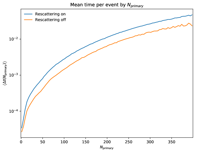
(a)

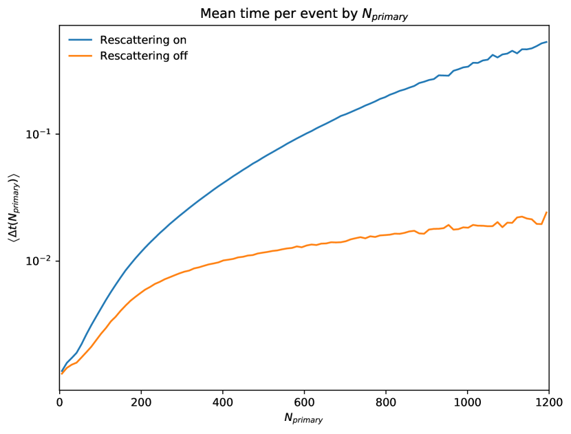
(b)

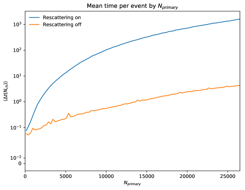
(c)

Figure 16: The average generation time of each event with a specified primary hadron multiplicity, for (a) $\mathrm{p}\mathrm{p}$, (b) $\mathrm{p}\mathrm{Pb}$ and (c) $\mathrm{Pb}\mathrm{Pb}$, with $\sqrt{s_{\mathrm{N}\mathrm{N}}}=5.02$ TeV.

References

- [1] M. L. Miller, K. Reygers, S. J. Sanders, and P. Steinberg, “Glauber modeling in high energy nuclear collisions,” Ann. Rev. Nucl. Part. Sci. 57 (2007) 205–243, nucl-ex/0701025.
- [2] P. Bożek, W. Broniowski, and M. Rybczyński, “Wounded quarks in A+A, p+A, and p+p collisions,” Phys. Rev. C 94 (2016), no. 1 014902, 1604.07697.
- [3] F. Gelis, E. Iancu, J. Jalilian-Marian, and R. Venugopalan, “The Color Glass Condensate,” Ann. Rev. Nucl. Part. Sci. 60 (2010) 463–489, 1002.0333.
- [4] B. Schenke, P. Tribedy, and R. Venugopalan, “Fluctuating Glasma initial conditions and flow in heavy ion collisions,” Phys. Rev. Lett. 108 (2012) 252301, 1202.6646.
- [5] A. Kurkela, A. Mazeliauskas, J.-F. Paquet, S. Schlichting, and D. Teaney, “Matching the Nonequilibrium Initial Stage of Heavy Ion Collisions to Hydrodynamics with QCD Kinetic Theory,” Phys. Rev. Lett. 122 (2019), no. 12 122302, 1805.01604.
- [6] U. Heinz and R. Snellings, “Collective flow and viscosity in relativistic heavy-ion collisions,” Ann. Rev. Nucl. Part. Sci. 63 (2013) 123–151, 1301.2826.
- [7] M. Luzum and H. Petersen, “Initial State Fluctuations and Final State Correlations in Relativistic Heavy-Ion Collisions,” J. Phys. G 41 (2014) 063102, 1312.5503.
- [8] C. Gale, S. Jeon, and B. Schenke, “Hydrodynamic Modeling of Heavy-Ion Collisions,” Int. J. Mod. Phys. A 28 (2013) 1340011, 1301.5893.
- [9] R. D. Weller and P. Romatschke, “One fluid to rule them all: viscous hydrodynamic description of event-by-event central p+p, p+Pb and Pb+Pb collisions at TeV,” Phys. Lett. B 774 (2017) 351–356, 1701.07145.
- [10] CMS Collaboration, V. Khachatryan et. al., “Observation of Long-Range Near-Side Angular Correlations in Proton-Proton Collisions at the LHC,” JHEP 09 (2010) 091, 1009.4122.
- [11] ATLAS Collaboration, G. Aad et. al., “Observation of Long-Range Elliptic Azimuthal Anisotropies in 13 and 2.76 TeV Collisions with the ATLAS Detector,” Phys. Rev. Lett. 116 (2016), no. 17 172301, 1509.04776.
- [12] CMS Collaboration, V. Khachatryan et. al., “Evidence for collectivity in pp collisions at the LHC,” Phys. Lett. B 765 (2017) 193–220, 1606.06198.
- [13] ALICE Collaboration, S. Acharya et. al., “Investigations of Anisotropic Flow Using Multiparticle Azimuthal Correlations in pp, p-Pb, Xe-Xe, and Pb-Pb Collisions at the LHC,” Phys. Rev. Lett. 123 (2019), no. 14 142301, 1903.01790.
- [14] ALICE Collaboration, J. Adam et. al., “Enhanced production of multi-strange hadrons in high-multiplicity proton-proton collisions,” Nature Phys. 13 (2017) 535–539, 1606.07424.
- [15] K. Werner, “Core-corona separation in ultra-relativistic heavy ion collisions,” Phys. Rev. Lett. 98 (2007) 152301, 0704.1270.
- [16] T. Pierog, I. Karpenko, J. Katzy, E. Yatsenko, and K. Werner, “EPOS LHC: Test of collective hadronization with data measured at the CERN Large Hadron Collider,” Phys. Rev. C 92 (2015), no. 3 034906, 1306.0121.
- [17] C. Bierlich, G. Gustafson, and L. Lönnblad, “Diffractive and non-diffractive wounded nucleons and final states in pA collisions,” JHEP 10 (2016) 139, 1607.04434.
- [18] C. Bierlich, G. Gustafson, L. Lönnblad, and H. Shah, “The Angantyr model for Heavy-Ion Collisions in PYTHIA8,” JHEP 10 (2018) 134, 1806.10820.
- [19] T. Sjöstrand, S. Mrenna, and P. Z. Skands, “PYTHIA 6.4 Physics and Manual,” JHEP 05 (2006) 026, hep-ph/0603175.
- [20] T. Sjöstrand, S. Ask, J. R. Christiansen, R. Corke, N. Desai, P. Ilten, S. Mrenna, S. Prestel, C. O. Rasmussen, and P. Z. Skands, “An introduction to PYTHIA 8.2,” Comput. Phys. Commun. 191 (2015) 159–177, 1410.3012.
- [21] B. Andersson, G. Gustafson, and B. Nilsson-Almqvist, “A Model for Low p(t) Hadronic Reactions, with Generalizations to Hadron - Nucleus and Nucleus-Nucleus Collisions,” Nucl. Phys. B 281 (1987) 289–309.
- [22] B. Andersson, G. Gustafson, and H. Pi, “The FRITIOF model for very high-energy hadronic collisions,” Z. Phys. C 57 (1993) 485–494.
- [23] C. Bierlich, G. Gustafson, and L. Lönnblad, “A shoving model for collectivity in hadronic collisions,” 1612.05132.
- [24] C. Bierlich, G. Gustafson, and L. Lönnblad, “Collectivity without plasma in hadronic collisions,” Phys. Lett. B 779 (2018) 58–63, 1710.09725.
- [25] C. Bierlich, S. Chakraborty, G. Gustafson, and L. Lönnblad, “Setting the string shoving picture in a new frame,” 2010.07595.
- [26] C. Bierlich, G. Gustafson, L. Lönnblad, and A. Tarasov, “Effects of Overlapping Strings in pp Collisions,” JHEP 03 (2015) 148, 1412.6259.
- [27] S. Bass et. al., “Microscopic models for ultrarelativistic heavy ion collisions,” Prog. Part. Nucl. Phys. 41 (1998) 255–369, nucl-th/9803035.
- [28] J. Weil et. al., “Particle production and equilibrium properties within a new hadron transport approach for heavy-ion collisions,” Phys. Rev. C 94 (2016), no. 5 054905, 1606.06642.
- [29] S. Ferreres-Solé and T. Sjöstrand, “The space–time structure of hadronization in the Lund model,” Eur. Phys. J. C 78 (2018), no. 11 983, 1808.04619.
- [30] A. V. da Silva, W. M. Serenone, D. Dobrigkeit Chinellato, J. Takahashi, and C. Bierlich, “Studies of heavy-ion collisions using PYTHIA Angantyr and UrQMD,” 2002.10236.
- [31] T. Sjöstrand and M. Utheim, “A Framework for Hadronic Rescattering in pp Collisions,” Eur. Phys. J. C 80 (2020), no. 10 907, 2005.05658.
- [32] W. Broniowski, M. Rybczynski, and P. Bozek, “GLISSANDO: Glauber initial-state simulation and more..,” Comput. Phys. Commun. 180 (2009) 69–83, 0710.5731.
- [33] M. Rybczynski, G. Stefanek, W. Broniowski, and P. Bozek, “GLISSANDO 2 : GLauber Initial-State Simulation AND mOre…, ver. 2,” Comput. Phys. Commun. 185 (2014) 1759–1772, 1310.5475.
- [34] G. A. Schuler and T. Sjöstrand, “Hadronic diffractive cross-sections and the rise of the total cross-section,” Phys. Rev. D 49 (1994) 2257–2267.
- [35] T. Sjöstrand and M. van Zijl, “A Multiple Interaction Model for the Event Structure in Hadron Collisions,” Phys. Rev. D 36 (1987) 2019.
- [36] T. Sjöstrand, “The Development of MPI Modeling in Pythia,” Adv. Ser. Direct. High Energy Phys. 29 (2018) 191–225, 1706.02166.
- [37] C. Bierlich and C. O. Rasmussen, “Dipole evolution: perspectives for collectivity and A collisions,” JHEP 10 (2019) 026, 1907.12871.
- [38] T. Sjöstrand and P. Z. Skands, “Multiple interactions and the structure of beam remnants,” JHEP 03 (2004) 053, hep-ph/0402078.
- [39] B. Andersson, G. Gustafson, G. Ingelman, and T. Sjöstrand, “Parton Fragmentation and String Dynamics,” Phys. Rept. 97 (1983) 31–145.
- [40] G. ’t Hooft, “A Planar Diagram Theory for Strong Interactions,” Nucl. Phys. B 72 (1974) 461.
- [41] T. Sjöstrand, “Jet Fragmentation of Nearby Partons,” Nucl. Phys. B 248 (1984) 469–502.
- [42] Z. Xu and C. Greiner, “Thermalization of gluons in ultrarelativistic heavy ion collisions by including three-body interactions in a parton cascade,” Phys. Rev. C 71 (2005) 064901, hep-ph/0406278.
- [43] R. Garcia-Martin, R. Kaminski, J. Pelaez, J. Ruiz de Elvira, and F. Yndurain, “The Pion-pion scattering amplitude. IV: Improved analysis with once subtracted Roy-like equations up to 1100 MeV,” Phys. Rev. D 83 (2011) 074004, 1102.2183.
- [44] J. Pelaez, A. Rodas, and J. Ruiz De Elvira, “Global parameterization of scattering up to 2 ,” Eur. Phys. J. C 79 (2019), no. 12 1008, 1907.13162.
- [45] J. Pelaez and A. Rodas, “Pion-kaon scattering amplitude constrained with forward dispersion relations up to 1.6 GeV,” Phys. Rev. D 93 (2016), no. 7 074025, 1602.08404.
- [46] Particle Data Group Collaboration, M. Tanabashi et. al., “Review of Particle Physics,” Phys. Rev. D 98 (2018), no. 3 030001.
- [47] Particle Data Group Collaboration, L. Montanet et. al., “Review of particle properties. Particle Data Group,” Phys. Rev. D 50 (1994) 1173–1823.
- [48] P. Koch and C. Dover, “, and Production in Relativistic Heavy Ion Collisions,” Phys. Rev. C 40 (1989) 145–155.
- [49] G. A. Schuler and T. Sjöstrand, “A Scenario for high-energy gamma gamma interactions,” Z. Phys. C 73 (1997) 677–688, hep-ph/9605240.
- [50] E. Levin and L. Frankfurt, “The Quark hypothesis and relations between cross-sections at high-energies,” JETP Lett. 2 (1965) 65–70.
- [51] H. J. Lipkin, “Quarks for pedestrians,” Phys. Rept. 8 (1973) 173–268.
- [52] ALICE Collaboration, J. Adam et. al., “Measurement of pion, kaon and proton production in proton–proton collisions at TeV,” Eur. Phys. J. C 75 (2015), no. 5 226, 1504.00024.
- [53] N. Fischer and T. Sjöstrand, “Thermodynamical String Fragmentation,” JHEP 01 (2017) 140, 1610.09818.
- [54] ALICE Collaboration, S. Acharya et. al., “Pion-kaon femtoscopy and the lifetime of the hadronic phase in PbPb collisions at = 2.76 TeV,” Phys. Lett. B 813 (2021) 136030, 2007.08315.
- [55] ALICE Collaboration, S. Acharya et. al., “Evidence of rescattering effect in Pb-Pb collisions at the LHC through production of and mesons,” Phys. Lett. B 802 (2020) 135225, 1910.14419.
- [56] C. Bierlich and J. R. Christiansen, “Effects of color reconnection on hadron flavor observables,” Phys. Rev. D 92 (2015), no. 9 094010, 1507.02091.
- [57] ALICE Collaboration, S. Acharya et. al., “Centrality and transverse momentum dependence of inclusive J/ production at midrapidity in Pb-Pb collisions at = 5.02 TeV,” Phys. Lett. B 805 (2020) 135434, 1910.14404.
- [58] S. Voloshin and Y. Zhang, “Flow study in relativistic nuclear collisions by Fourier expansion of Azimuthal particle distributions,” Z. Phys. C 70 (1996) 665–672, hep-ph/9407282.
- [59] A. M. Poskanzer and S. A. Voloshin, “Methods for analyzing anisotropic flow in relativistic nuclear collisions,” Phys. Rev. C 58 (1998) 1671–1678, nucl-ex/9805001.
- [60] ALICE Collaboration, B. B. Abelev et. al., “Azimuthal anisotropy of D meson production in Pb-Pb collisions at TeV,” Phys. Rev. C 90 (2014), no. 3 034904, 1405.2001.
- [61] ALICE Collaboration, E. Abbas et. al., “J/Psi Elliptic Flow in Pb-Pb Collisions at = 2.76 TeV,” Phys. Rev. Lett. 111 (2013) 162301, 1303.5880.
- [62] C. Bierlich et. al., “Robust Independent Validation of Experiment and Theory: Rivet version 3,” SciPost Phys. 8 (2020) 026, 1912.05451.
- [63] ALICE Collaboration, K. Aamodt et. al., “Centrality dependence of the charged-particle multiplicity density at mid-rapidity in Pb-Pb collisions at TeV,” Phys. Rev. Lett. 106 (2011) 032301, 1012.1657.
- [64] ALICE Collaboration, E. Abbas et. al., “Centrality dependence of the pseudorapidity density distribution for charged particles in Pb-Pb collisions at = 2.76 TeV,” Phys. Lett. B 726 (2013) 610–622, 1304.0347.
- [65] ALICE Collaboration, B. Abelev et. al., “Centrality Dependence of Charged Particle Production at Large Transverse Momentum in Pb–Pb Collisions at TeV,” Phys. Lett. B 720 (2013) 52–62, 1208.2711.
- [66] D. Teaney and L. Yan, “Triangularity and Dipole Asymmetry in Heavy Ion Collisions,” Phys. Rev. C 83 (2011) 064904, 1010.1876.
- [67] A. Bilandzic, C. H. Christensen, K. Gulbrandsen, A. Hansen, and Y. Zhou, “Generic framework for anisotropic flow analyses with multiparticle azimuthal correlations,” Phys. Rev. C 89 (2014), no. 6 064904, 1312.3572.
- [68] C. Bierlich et. al., “Confronting experimental data with heavy-ion models: RIVET for heavy ions,” Eur. Phys. J. C 80 (2020), no. 5 485, 2001.10737.
- [69] P. Huo, K. Gajdošová, J. Jia, and Y. Zhou, “Importance of non-flow in mixed-harmonic multi-particle correlations in small collision systems,” Phys. Lett. B 777 (2018) 201–206, 1710.07567.
- [70] J. Auvinen and H. Petersen, “Evolution of elliptic and triangular flow as a function of in a hybrid model,” Phys. Rev. C 88 (2013), no. 6 064908, 1310.1764.
- [71] P. Dorau, J.-B. Rose, D. Pablos, and H. Elfner, “Jet Quenching in the Hadron Gas: An Exploratory Study,” Phys. Rev. C 101 (2020), no. 3 035208, 1910.07027.
- [72] STAR Collaboration, C. Adler et. al., “Disappearance of back-to-back high hadron correlations in central Au+Au collisions at = 200-GeV,” Phys. Rev. Lett. 90 (2003) 082302, nucl-ex/0210033.
- [73] ALICE Collaboration, K. Aamodt et. al., “Particle-yield modification in jet-like azimuthal di-hadron correlations in Pb-Pb collisions at TeV,” Phys. Rev. Lett. 108 (2012) 092301, 1110.0121.
- [74] P. Lebiedowicz and A. Szczurek, “Production of meson in collisions at the LHC via gluon-gluon fusion in the -factorization approach,” Phys. Lett. B 810 (2020) 135816, 2007.12485.
- [75] L. A. Dal and A. R. Raklev, “Alternative formation model for antideuterons from dark matter,” Phys. Rev. D 91 (2015), no. 12 123536, 1504.07242. [Erratum: Phys.Rev.D 92, 069903 (2015), Erratum: Phys.Rev.D 92, 089901 (2015)].