An open-source ABAQUS implementation of the scaled boundary finite element method to study interfacial problems using polyhedral meshes

Abstract

The scaled boundary finite element method (SBFEM) is capable of generating polyhedral elements with an arbitrary number of surfaces. This salient feature significantly alleviates the meshing burden being a bottleneck in the analysis pipeline in the standard finite element method (FEM). In this paper, we implement polyhedral elements based on the SBFEM into the commercial finite element software ABAQUS. To this end, user elements are provided through the user subroutine UEL. Detailed explanations regarding the data structures and implementational aspects of the procedures are given. The focus of the current implementation is on interfacial problems and therefore, element-based surfaces are created on polyhedral user elements to establish interactions. This is achieved by an overlay of standard finite elements with negligible stiffness, provided in the ABAQUS element library, with polyhedral user elements. By means of several numerical examples, the advantages of polyhedral elements regarding the treatment of non-matching interfaces and automatic mesh generation are clearly demonstrated. Thus, the performance of ABAQUS for problems involving interfaces is augmented based on the availability of polyhedral meshes. Due to the implementation of polyhedral user elements, ABAQUS can directly handle complex geometries given in the form of digital images or stereolithography (STL) files. In order to facilitate the use of the proposed approach, the code of the UEL is published open-source and can be downloaded from https://github.com/ShukaiYa/SBFEM-UEL.

1 Introduction

The finite element method (FEM) has been widely used in engineering and science for solving partial differential equations arising in many different areas of application. To this end, the FEM discretizes a problem domain into a number of subdomains of simple shape, so-called finite elements, and assembles them to derive numerical solutions. Geometrically simple elements are commonly utilized in the standard FEM, e.g., tetrahedral and hexahedral elements in three-dimensional applications. Many commercial finite element software packages are available, such as ANSYS, ABAQUS, MARC, etc. which makes the FEM easily accessible for engineers and researchers alike. Nonetheless, there are some aspects that the FEM is unable to handle in a satisfactory manner: a) stress singularities occurring in fracture mechanics problems [1] and b) the representation of the unbounded domains [2]. Additionally, mesh generation is still laborious and time-consuming and therefore, often constitutes a severe bottleneck in the analysis pipeline. Considering special data formats, such as digital images and stereolithography (STL), which are nowadays widely adopted by industry, this problem is prominent. To alleviate the aforementioned issues, various alternatives have been proposed by researchers, to name a few, the boundary element method (BEM) [3], the scaled boundary finite element method (SBFEM) [4], and the extended finite element method (X-FEM) [5].

The SBFEM is in its core nature a semi-analytical method which was first proposed by Wolf and Song [4, 6] for modeling wave propagation in unbounded domains. However, over the last two decades, the SBFEM has been extended to various types of analyses including wave propagation in bounded domains [7], fracture mechanics [8, 9, 10], acoustics [11, 12], contact mechanics [13, 14], seepage [15], elasto-plasticity [16], damage analysis [17], adaptive analysis [18, 19], among many others [20, 21, 22, 23]. Due to its versatility and applicability to a wide class of problems, the SBFEM can be seen as a general numerical method to solve PDEs.

One of the main advantages of SBFEM over standard FEM is that it offers greater flexibility regarding the spatial discretization, as polytope elements of an arbitrary number of vertices, edges and surfaces can be straightforwardly constructed. This advantage significantly reduces the meshing burden encountered in the standard FEM. Firstly, the SBFEM is highly complementary to the hierarchical tree-based mesh generation technique, which is a robust mesh generation technology that can automatically discretize complicated geometries with highly irregular boundaries [24, 25, 26]. In recent years, such polytope elements have been employed in SBFEM analyses for both two- [27] and three-dimensional [28, 29] problems. The geometry can be either stored as digital images obtained from computed tomography (CT) scans or as STL files widely used in 3D printing. Secondly, the polytope elements allow meshes with rapid transitions in element size, which is beneficial for the modeling of complex domains [30]. To obtain analysis-ready meshes for complex structures, such as particle reinforced composites, human bones, or other micro-structured materials, the geometric details of the structure require small element sizes at the boundary, while in the interior larger elements are appropriate. Hence, we require transition elements allowing adjacent polytope elements with different sizes, effectively reducing the number of elements and also the computational resources required. Finally, owing to the higher degree of flexibility of polytope elements, the initially non-matching interface meshes can be straightforwardly converted to matching ones by splitting interface edges (2D) or surfaces (3D) [31]. The matching discretization on the interface benefits the analyses involving multiple domains by facilitating the application of interface constraints. Common areas of application include domain decomposition [31], contact [13, 14], and acoustic-structure interaction [32] problems.

Despite the aforementioned advantages of the SBFEM, the popularity of this method is still restricted to a small part of the scientific community. One important reason is seen in the more involved theoretical derivation of the SBFEM compared to the FEM. The FEM is practically taught in any engineering program at universities all over the world, concise mathematical theories on its properties exist, and powerful commercial software packages are readily available, while the SBFEM has been so far only implemented for research purposes. With the implementation of the SBFEM into a commercial software package, experienced analysts will have easy access to SBFEM and can exploit its advantages. It is our intent to facilitate the acceptance of the method itself and spark its further development to other classes of problems. Considering scholars interested in starting research on the SBFEM, the availability of the implementation will provide a user-friendly and robust platform and comprehensive access to non-linear solvers.

The possibility of implementing other numerical methods which are related to the FEM into commercial software packages provides a whole new set of possibilities and can be realized through programming user element subroutines. Many commercial FEM codes support this functionality, e.g., $\mathrm{USERELEM}$ in ANSYS [33], $\mathrm{USELEM}$ in MARC [34], and $\mathrm{UEL}$ in ABAQUS [35]. In recent years, many non-standard numerical methods have been implemented in ABAQUS. Before the X-FEM was available as an additional module of commercial software packages, it was implemented in the form of a user element [36, 37, 38]. Elguedj et al. [39] introduced the user element implementation of NURBS based on isogeometric analysis. The cell-based smoothed finite element method (CSFEM) was implemented as user elements in ABAQUS by Cui et al. [40] and Kumbhar et al. [41] for alleviating mesh distortion issues seen in standard finite elements. Yang et al. [42] implemented the SBFEM in ABAQUS and showed the benefits of using polytope (polygon/polyhedron) elements in linear elastic stress analyses.

In the article at hand, linear elastic polyhedral element straightforwardly constructed by the SBFEM is implemented into ABAQUS through $\mathrm{UEL}$. To be consistent with ABAQUS’ element library, the surfaces of polyhedral element are discretized only as triangular and quadrilateral shapes, and only low-order (linear and quadratic) finite elements are used for the surface tessellation in this paper. In this way, the SBFEM and FEM can be easily coupled since the discretization of element surfaces is identical. In addition, another ABAQUS’ user subroutine, $\mathrm{UEXTERNALDB}$ to manage external databases, is involved in the current implementation. Because of the arbitrariness of polyhedron in terms of topology, the nodal connectivity of the polyhedral user element should be recovered by a supplementary input file. The $\mathrm{UEXTERNALDB}$ is used to open the supplementary input file and store the polyhedral mesh information in a memory-efficient way.

The main goal of this paper is to illustrate the advantages of the SBFEM user element with a special focus on three-dimensional interfacial problems. For this type of applications, some salient features of ABAQUS can be utilized, such as i) the comprehensive approaches for the contact modeling, ii) enriched library of cohesive elements for the modeling of interfacial behaviors, and iii) powerful non-linear solution techniques. It is also our belief that ABAQUS can benefit from the salient features of the SBFEM in different aspects mentioned in the previous paragraphs. In addition to a more flexible meshing paradigm provided by the SBFEM, the performance of ABAQUS can be enhanced for further specific applications. ABAQUS models containing non-matching interface meshes, e.g., fail to pass the patch test both in domain decomposition [31] and contact [13, 14] problems, especially when the interfaces are curved. Using polytope elements, the theoretical results are recovered again, as we can easily generate matching surfaces for a wide variety of cases.

The remaining part of this paper is organized as follows: A brief review of the theoretical derivations of the SBFEM is presented in Section 2. Section 3 introduces the implementation of the SBFEM user element in ABAQUS, including its workflow, ABAQUS input file formats, data structures for storing the mesh information, a detailed explanation of the implementation and the definition of element-based surfaces needed for contact modeling. The numerical examples include academic benchmark tests and more complex structures clearly demonstrating the main advantages of the SBFEM (see Section 4). Finally, important conclusions are provided in Section 5.

2 Theory of the scaled boundary finite element method

This section briefly summarizes the construction of polyhedral elements using SBFEM. Only the key concepts and equations related to the implementation of the SBFEM as a user element are presented. Readers interested in detailed discussions and derivations of this method are referred to the monograph by Song [43].

2.1 Polyhedral elements in the SBFEM

Polyhedral elements offer a great deal of flexibility in terms of mesh generation and mesh transitioning, especially for geometrically complex structures and adaptive analyses. One of the salient features of SBFEM is that we can straightforwardly derive such elements. In general, a polyhedral mesh can be created by discretizing the boundary into surface elements, while the volume of the domain is not discretized itself [4]. A typical example of a polyhedral element employing the SBFEM is illustrated in Fig. 1. A so-called scaling center (denoted as “$\mathbf{\mathit{O}}$” in Fig. 1a) is selected within the volume, such that every point on the boundary is directly visible, i.e., the domain has to fulfill the requirements of star-convexity. The boundary of the polyhedral domain is discretized using surface elements, which are commonly of triangular and quadrilateral shapes as depicted in Fig. 1b. The volume of the polyhedral mesh is represented by scaling the surface elements towards the scaling center. Only the solution on surface elements is interpolated whereas the solution inside the polyhedral element will be obtained analytically, leading to a semi-analytical procedure.

(a) Volume and scaling center

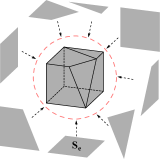
(b) Surface descretization

Figure 1: Schematic of a polyhedral mesh

It is worthwhile to mention that in the framework of the SBFEM, often standard low-order finite elements are used for the surface tessellation, although high-order elements [44] and arbitrary faceted polyhedra [45] are possible. Besides, because it is well-known that quadrilateral elements generally perform better than triangular elements due to the additional higher-order terms in the approximation space, an approach to avoid the use of triangular elements in the surface discretization is proposed [46]. To be consistent with ABAQUS’ element library, we only add linear and quadratic triangular (T3 and T6) and quadrilateral (Q4 and Q8) elements in the current implementation. In the numerical examples presented in Section 4, only linear elements are used.

2.2 Geometry transformation

The geometry transformation in the SBFEM is formulated by combining the boundary discretization with a scaling operation of the boundary. The scaling procedure is illustrated in Fig. 2a for a quadrilateral surface element. A volume sector $\mathrm{V}_{\mathrm{e}}$ is represented by continuously scaling the surface element $\mathrm{S}_{\mathrm{e}}$ to the scaling center. A three-dimensional scaled boundary coordinate system is established in each volume sector, with the circumferential coordinates $\eta$, $\zeta$ on the surface element and the radial coordinate $\xi$.

The surface elements on the boundary are isoparametric elements known from the standard FEM [47]. The most commonly used triangular and quadrilateral elements are depicted in Fig. 2b in its natural coordinates $\eta$, $\zeta$. The nodes marked in red are only used for quadratic elements. The surface element’s shape functions are denoted by $\mathrm{\mathbf{N}}(\eta,\zeta)$. The radial coordinate $\mathit{\xi}$ is dimensionless, emanating from the scaling center and pointing towards the boundary. At the scaling center $\xi=0$ and on the boundary $\xi=1$ hold.

(a) Scaling of the surface element using radial coordinate $\xi$ ($\xi=0$ at the scaling center and $\xi=1$ on the boundary)

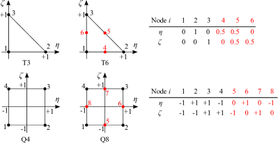
(b) Triangular and quadrilateral reference elements in natural coordinates $\eta$, $\zeta$

Figure 2: Three-dimensional scaled boundary coordinate system

A point ($\hat{x},\hat{y},\hat{z}$) within the volume sector $\mathrm{V}_{\mathrm{e}}$ can be defined by the scaled boundary coordinates ($\eta,\zeta,\xi$) as:

$$\hat{x}(\xi,\eta,\zeta)=\xi\hat{x}(\eta,\zeta)=\xi\mathbf{N}(\eta,\zeta)\hat{\mathbf{x}},$$ (1a)

$$\hat{y}(\xi,\eta,\zeta)=\xi\hat{y}(\eta,\zeta)=\xi\mathbf{N}(\eta,\zeta)\hat{\mathbf{y}},$$ (1b)

$$\hat{z}(\xi,\eta,\zeta)=\xi\hat{z}(\eta,\zeta)=\xi\mathbf{N}(\eta,\zeta)\hat{\mathbf{z}},$$ (1c)

where $\hat{\mathbf{x}}$, $\hat{\mathbf{y}}$ and $\hat{\mathbf{z}}$ are the nodal coordinate vectors of the surface element $\mathrm{S}_{\mathrm{e}}$ in Cartesian coordinates. Note that all the coordinates in Eq. (1) are the relative coordinates with respect to the scaling center, i.e., the scaling center is taken as the origin of the local coordinate system, and the hat symbol over variables indicates that they are related to this specific local coordinate systems.

The partial derivatives with respect to the scaled boundary coordinates can be related to the partial derivatives in Cartesian coordinates by the following equation:

$$\left\{\begin{array}[]{c}\frac{\partial}{\partial\xi}\\ \frac{\partial}{\partial\eta}\\ \frac{\partial}{\partial\zeta}\end{array}\right\}=\left[\begin{array}[]{ccc}1&0&0\\ 0&\xi&0\\ 0&0&\xi\end{array}\right]\mathbf{J}_{\mathrm{b}}(\eta,\zeta)\left\{\begin{array}[]{c}\frac{\partial}{\partial x}\\ \frac{\partial}{\partial y}\\ \frac{\partial}{\partial z}\end{array}\right\},$$ (2)

where $\mathbf{J}_{\mathrm{b}}(\eta,\zeta)$ denotes the Jacobian matrix on the boundary ($\xi=1$), which is defined as

$$\mathbf{J}_{\mathrm{b}}(\eta,\zeta)=\left[\begin{array}[]{ccc}\hat{x}(\eta,\zeta)&\hat{y}(\eta,\zeta)&\hat{z}(\eta,\zeta)\\ \hat{x}(\eta,\zeta)_{,\eta}&\hat{y}(\eta,\zeta)_{,\eta}&\hat{y}(\eta,\zeta)_{,\eta}\\ \hat{x}(\eta,\zeta)_{,\zeta}&\hat{y}(\eta,\zeta)_{,\zeta}&\hat{z}(\eta,\zeta)_{,\zeta}\end{array}\right].$$ (3)

The determinant of $\mathbf{J}_{\mathrm{b}}(\eta,\zeta)$ is given as

$$\left|\mathbf{J}_{\mathrm{b}}\right|=\hat{x}(\hat{y}_{,\eta}\hat{z}_{,\zeta}-\hat{z}_{,\eta}\hat{y}_{,\zeta})+\hat{y}(\hat{z}_{,\eta}\hat{x}_{,\zeta}-\hat{x}_{,\eta}\hat{z}_{,\zeta})+\hat{z}(\hat{x}_{,\eta}\hat{y}_{,\zeta}-\hat{y}_{,\eta}\hat{x}_{,\zeta}),$$ (4)

where the argument ($\eta,\zeta$) has been dropped for the sake of clarity.

2.2.1 Displacement field

As a semi-analytical procedure, the SBFEM introduces unknown nodal displacement functions $\mathbf{u}^{\mathrm{e}}(\xi)$ for the representation of the displacement field of a volume sector $\mathrm{V}_{\mathrm{e}}$in radial direction, i.e., those functions express the displacements along the radial lines connecting the scaling center and boundary nodes on e-th surface element $\mathrm{S}_{\mathrm{e}}$, and they are usually determined analytically. For the sake of completeness, we remark that in Refs. [48, 49] a numerical approximation in radial direction has been successfully established.

The displacements at a point ($\xi,\eta,\zeta$) within the volume sector $\mathrm{V}_{\mathrm{e}}$ are interpolated based on $\mathbf{u}^{\mathrm{e}}(\xi)$, thus the displacement field $\mathrm{\mathbf{u}}(\xi,\eta,\zeta)$ is expressed as

$$\mathrm{\mathbf{u}}(\xi,\eta,\zeta)=\mathbf{N}_{\mathrm{u}}(\eta,\zeta)\mathbf{u}^{\mathrm{e}}(\xi),$$ (5)

where the shape function matrix $\mathbf{N}_{\mathrm{u}}(\eta,\zeta)$ is written as

$$\mathbf{N}_{\mathrm{u}}(\eta,\zeta)=\left[N_{1}(\eta,\zeta)\mathbf{I},N_{2}(\eta,\zeta)\mathbf{I},\cdots,N_{n}(\eta,\zeta)\mathbf{I}\right],$$ (6)

with a $3\times 3$ identity matrix $\mathbf{I}$.

The nodal displacement functions $\mathbf{u}(\xi)$ of the entire element are assembled by

$$\mathbf{u}(\xi)=\underset{e}{\mathrm{\mathbb{A}}}\mathop{\mathbf{u}^{\mathrm{e}}(\xi)},$$ (7)

where the symbol $\underset{e}{\mathrm{\mathbb{A}}}$ indicates the standard finite element assembly procedure.

2.2.2 Strain field

In scaled boundary coordinates, the strain field $\boldsymbol{\boldsymbol{\varepsilon}}(\xi,\eta,\zeta)$ is obtained from the displacement field $\mathrm{\mathbf{u}}(\xi,\eta,\zeta)$ by applying the linear differential operator $\mathbf{L}$

$$\boldsymbol{\boldsymbol{\varepsilon}}(\xi,\eta,\zeta)=\mathbf{L}\mathrm{\mathbf{u}}(\xi,\eta,\zeta),$$ (8)

which is defined by

$$\mathbf{L}=\mathbf{b}_{1}(\eta,\zeta)\frac{\partial}{\partial\xi}+\frac{1}{\xi}\left(\mathbf{b}_{2}(\eta,\zeta)\frac{\partial}{\partial\eta}+\mathbf{b}_{3}(\eta,\zeta)\frac{\partial}{\partial\zeta}\right),$$ (9)

where the matrices $\mathbf{b}_{1}(\eta,\zeta)$, $\mathbf{b}_{2}(\eta,\zeta)$, $\mathbf{b}_{3}(\eta,\zeta)$ can be found in Ref. [43], their entries are taken directly from the inverse of the Jacobian matrix $\mathbf{J}_{\mathrm{b}}$. Substituting Eq. (5) into Eq. (8), the relationship between the strain field and the nodal displacement functions can be obtained as

$$\boldsymbol{\boldsymbol{\varepsilon}}(\xi,\eta,\zeta)=\mathbf{B}_{1}(\eta,\zeta)\mathrm{\mathbf{u}}(\xi)_{,\xi}+\frac{1}{\text{$\xi$}}\mathbf{B}_{2}(\eta,\zeta)\mathrm{\mathbf{u}}(\xi),$$ (10)

where

$$\mathbf{B}_{1}(\eta,\zeta)=\mathbf{b}_{1}(\eta,\zeta)\mathbf{N}_{\mathrm{u}}(\eta,\zeta),$$ (11a)

$$\mathbf{B}_{2}(\eta,\zeta)=\mathbf{b}_{2}(\eta,\zeta)\mathbf{N}_{\mathrm{u}}(\eta,\zeta)_{,\eta}+\mathbf{b}_{3}(\eta,\zeta)\mathbf{N}_{\mathrm{u}}(\eta,\zeta)_{,\zeta}.$$ (11b)

2.2.3 Stress field

For linear elastic problems, the stress field $\boldsymbol{\sigma}(\xi,\eta,\zeta)$ is related to the strain field by

$$\boldsymbol{\sigma}(\xi,\eta,\zeta)=\mathbf{D}\boldsymbol{\boldsymbol{\varepsilon}}(\xi,\eta,\zeta),$$ (12)

where $\mathbf{D}$ is the elasticity matrix, which is expressed as follows for linear isotropic material:

$$\mathbf{D}=\frac{E}{(1+\nu)(1-2\nu)}\left[\begin{array}[]{cccccc}1-\nu&\nu&\nu&0&0&0\\ &1-\nu&\nu&0&0&0\\ &&1-\nu&0&0&0\\ &&&\frac{1-2\nu}{2}&0&0\\ &&&&\frac{1-2\nu}{2}&0\\ &&\mathrm{Symmetric}&&&\frac{1-2\nu}{2}\end{array}\right].$$ (13)

Substituting Eq. (10) into Eq. (12), the relationship between the stress field and the nodal displacement functions can be expressed as

$$\boldsymbol{\sigma}(\xi,\eta,\zeta)=\mathbf{D}\left(\mathbf{B}_{1}(\eta,\zeta)\mathrm{\mathbf{u}}(\xi)_{,\xi}+\frac{1}{\text{$\xi$}}\mathbf{B}_{2}(\eta,\zeta)\mathrm{\mathbf{u}}(\xi)\right).$$

2.3 Scaled boundary finite element equation

By applying Galerkin’s method, the scaled boundary finite element equation in terms of nodal displacement functions is derived as

$$\mathbf{E}_{0}\xi^{2}\mathbf{u}(\xi)_{,\xi\xi}+\left(2\mathbf{E}_{0}-\mathbf{E}_{1}+\mathbf{E}_{1}^{\mathrm{T}}\right)\text{$\xi$}\mathbf{u}(\xi)_{,\xi}+\left(\mathbf{E}_{1}^{\mathrm{T}}-\mathbf{E}_{2}\right)\mathbf{u}(\xi)+\mathbf{P}(\xi)-\xi^{2}\mathbf{M}_{0}\ddot{\mathbf{u}}(\xi)=\mathbf{0}.$$ (14)

The coefficient matrices $\mathbf{E}_{0}$, $\mathbf{E}_{1}$, $\mathbf{E}_{2}$ and $\mathbf{M}_{0}$ of the entire element are assembled from the coefficient matrices $\mathbf{E}_{0}^{\mathrm{e}}$, $\mathbf{E}_{1}^{\mathrm{e}}$, $\mathbf{E}_{2}^{\mathrm{e}}$ and $\mathbf{M}_{0}^{\mathrm{e}}$ belonging to each surface element. The coefficient matrices $\mathbf{E}_{0}^{\mathrm{e}}$, $\mathbf{E}_{1}^{\mathrm{e}}$, $\mathbf{E}_{2}^{\mathrm{e}}$ and $\mathbf{M}_{0}^{\mathrm{e}}$ of a surface element $\mathrm{S}_{\mathrm{e}}$ are given as

$$\mathbf{E}_{0}^{\mathrm{e}}=\int_{\mathrm{S}_{\mathrm{e}}}\mathbf{B}_{1}^{\mathrm{T}}\mathbf{D}\mathbf{B}_{1}\left|\mathbf{J}_{\mathrm{b}}\right|\mathrm{d}\eta\mathrm{d}\zeta,$$ (15a)

$$\mathbf{E}_{1}^{\mathrm{e}}=\int_{\mathrm{S}_{\mathrm{e}}}\mathbf{B}_{2}^{\mathrm{T}}\mathbf{D}\mathbf{B}_{1}\left|\mathbf{J}_{\mathrm{b}}\right|\mathrm{d}\eta\mathrm{d}\zeta,$$ (15b)

$$\mathbf{E}_{2}^{\mathrm{e}}=\int_{\mathrm{S}_{\mathrm{e}}}\mathbf{B}_{2}^{\mathrm{T}}\mathbf{D}\mathbf{B}_{2}\left|\mathbf{J}_{\mathrm{b}}\right|\mathrm{d}\eta\mathrm{d}\zeta,$$ (15c)

$$\mathbf{M}_{0}^{\mathrm{e}}=\int_{\mathrm{S}_{\mathrm{e}}}\mathbf{N}_{\mathrm{u}}^{\mathrm{T}}\rho\mathbf{N}_{\mathrm{u}}\left|\mathbf{J}_{\mathrm{b}}\right|\mathrm{d}\eta\mathrm{d}\zeta,$$ (15d)

where $\rho$ is the mass density. The load function vector $\mathbf{P}(\xi)$ may include contributions due to surface traction, body forces, and initial stresses; readers are referred to Ref. [43] for details.

The system of non-homogeneous second-order ordinary differential equations (ODEs) in Eq. (14) can be transferred into a system of homogeneous first-order ODEs by doubling the number of unknowns and neglecting the inertial and external loads. The variable

$$\mathbf{X}(\xi)=\left[\begin{array}[]{c}\xi^{0.5}\mathrm{\mathbf{u}}(\xi)\\ \xi^{-0.5}\mathrm{\mathbf{q}}(\xi)\end{array}\right]$$ (16)

is introduced, where $\mathrm{\mathbf{q}}(\xi)$ denotes the vector of internal nodal force functions on a surface with constant $\xi$ and can be formulated as [43]

$$\mathbf{q}(\xi)=\xi\left(\mathbf{E}_{0}\xi\mathrm{\mathbf{u}}(\xi)_{,\xi}+\mathbf{E}_{1}^{\mathrm{T}}\mathrm{\mathbf{u}}(\xi)\right).$$ (17)

Substituting Eqs. (16) and (17) into Eq. (14), the scaled boundary finite element equation is reformulated as

$$\xi\mathbf{X}(\xi)_{,\xi}=\mathbf{Z}_{\mathrm{p}}\mathbf{X}(\xi),$$ (18)

where the coefficient matrix $\mathbf{\mathbf{Z}_{\mathrm{p}}}$ is a Hamiltonian matrix and defined as

$$\mathbf{Z}_{\mathrm{p}}=\left[\begin{array}[]{cc}-\mathbf{E}_{0}^{-1}\mathbf{E}_{1}^{\mathrm{T}}+0.5\mathbf{I}&\mathbf{E}_{0}^{-1}\\ \mathbf{E}_{2}-\mathbf{E}_{1}\mathbf{E}_{0}^{-1}\mathbf{E}_{1}^{\mathrm{T}}&\mathbf{E}_{1}\mathbf{E}_{0}^{-1}-0.5\mathbf{I}\end{array}\right].$$ (19)

2.4 Solution of the scaled boundary finite element equation

The scaled boundary finite element equation constitutes a system of Euler-Cauchy equations, see Eq. (18), which can be solved by applying eigenvalue or block-diagonal Schur decompositions [50]. The simpler eigenvalue method is utilized for the numerical implementation of our work, and therefore, a brief summary is presented in this subsection.

The eigenvalue problem of $\mathbf{Z}_{\mathrm{p}}$ can be expressed in matrix form as

$$\mathbf{Z}_{\mathrm{p}}\mathbf{\Phi}=\mathbf{\Phi}\mathbf{\Lambda},$$ (20)

where $\mathbf{\Phi}$ denotes the eigenvector matrix, and $\mathbf{\Lambda}$ is the diagonal matrix of eigenvalues. The general solution of $\mathbf{X}(\xi)$ is expressed as:

$$\mathbf{X}(\xi)=\mathbf{\Phi}\xi^{\mathbf{\text{$\Lambda$}}}\mathbf{C},$$ (21)

where $\mathbf{C}$ is the vector of integration constants which depends on the boundary conditions.

The general solution of $\mathbf{X}(\xi)$, given in Eq. (21), can be sorted by the real parts of the eigenvalues in descending order. It is well-known that if $\lambda$ is an eigenvalue of a Hamiltonian matrix, $-\lambda$ is also an eigenvalue of this particular matrix [51]. Thus, Eq. (21) can be rewritten as

$$\mathbf{X}(\xi)=\mathbf{\left[\begin{array}[]{cc}\mathbf{\Phi}_{\mathrm{u1}}&\mathbf{\Phi}_{\mathrm{u2}}\\ \mathbf{\Phi}_{\mathrm{q1}}&\mathbf{\Phi}_{\mathrm{q2}}\end{array}\right]}\left[\begin{array}[]{cc}\xi^{\mathbf{\Lambda}^{+}}&0\\ 0&\xi^{\mathbf{\Lambda}^{-}}\end{array}\right]\mathbf{\left[\begin{array}[]{c}\mathbf{C}_{\mathrm{1}}\\ \mathbf{C}_{\mathrm{2}}\end{array}\right]},$$ (22)

where $\mathbf{\Phi}_{\mathrm{u1}}$, $\mathbf{\Phi}_{\mathrm{u2}}$, $\mathbf{\Phi}_{\mathrm{q1}}$, and $\mathbf{\Phi}_{\mathrm{q2}}$ are the sub-matrices of $\mathbf{\Phi}$, and $\mathbf{\Lambda}^{+}$ and $\mathbf{\Lambda}^{-}$ are the diagonal matrices of eigenvalues with positive and negative real parts, respectively. $\mathbf{C}_{\mathrm{1}}$ and $\mathbf{C}_{\mathrm{2}}$ denote the vectors of integration constants related to $\mathbf{\Lambda}^{+}$ and $\mathbf{\Lambda}^{-}$, respectively. For bounded domains, the displacements have to remain finite inside the element and therefore, the integration constants contained in $\mathbf{C}_{2}$ have to be equal to zero. Otherwise the power function $\xi^{\mathbf{\Lambda}^{-}}$ would go to infinity near the scaling center ($\xi=0$). Consequently, the general solution given by Eq. (22) can be simplified as

$$\mathbf{X}(\xi)=\mathbf{\left[\begin{array}[]{c}\mathbf{\mathbf{\Phi}}_{\mathrm{u1}}\\ \mathbf{\mathbf{\Phi}}_{\mathrm{q1}}\end{array}\right]\xi^{\mathbf{\Lambda}^{+}}\mathbf{C}_{\mathrm{1}}}.$$ (23)

Using the definition of $\mathbf{X}(\xi)$ in Eq. (16) together with the general solution provided in Eq. (23), the unknown nodal displacement functions $\mathrm{\mathbf{u}}(\xi)$ and nodal force functions $\mathrm{\mathbf{q}}(\xi)$ can be expressed as

$$\mathbf{u}(\xi)=\mathbf{\mathbf{\Phi}}_{\mathrm{u1}}\xi^{\mathbf{\Lambda}^{+}-0.5\mathbf{I}}\mathbf{C}_{1},$$ (24a)

$$\mathbf{q}(\xi)=\mathbf{\mathbf{\Phi}}_{\mathrm{q1}}\xi^{\mathbf{\Lambda}^{+}+0.5\mathbf{I}}\mathbf{C}_{1}.$$ (24b)

The relationship between the nodal displacement functions and the nodal force functions can be obtained by eliminating the integration constants as

$$\mathbf{q}(\xi)=\mathbf{\mathbf{\Phi}}_{\mathrm{q1}}\mathbf{\mathbf{\Phi}}_{\mathrm{u1}}^{-1}\xi\mathbf{u}(\xi).$$ (25)

On the boundary ($\xi=1$), the nodal force vector $\mathbf{F}=\mathbf{q}(\xi=1)$ and the nodal displacement vector $\mathbf{d}=\mathbf{u}(\xi=1)$ apply. The relationship between nodal force and displacement vectors is $\mathbf{F=Kd}$, therefore, the stiffness matrix of the subdomain is expressed as

$$\mathbf{K}=\mathbf{\mathbf{\Phi}}_{\mathrm{q1}}\mathbf{\mathbf{\Phi}}_{\mathrm{u1}}^{-1}.$$ (26)

The mass matrix of a volume element is formulated as [43]

$$\mathbf{M}=\mathbf{\mathbf{\Phi}}_{\mathrm{u1}}^{-\mathrm{T}}\int_{0}^{1}\xi^{\mathbf{\Lambda}^{+}}\mathbf{m}_{0}\xi^{\mathbf{\Lambda}^{+}}\xi\mathrm{d}\xi\mathbf{\mathbf{\Phi}}_{\mathrm{u1}}^{-1},$$ (27)

where the coefficient matrix $\mathbf{m}_{0}$ is given by

$$\mathbf{m}_{0}=\mathbf{\mathbf{\Phi}}_{\mathrm{u1}}^{\mathrm{T}}\mathbf{M}_{0}\mathbf{\mathbf{\Phi}}_{\mathrm{u1}}.$$ (28)

Transferring the integration part in Eq. (27) into a matrix form, the expression of the mass matrix can be rewritten as

$$\mathbf{M}=\mathbf{\mathbf{\Phi}}_{\mathrm{u1}}^{-\mathrm{T}}\mathbf{m}\mathbf{\mathbf{\Phi}}_{\mathrm{u1}}^{-1},$$ (29)

where

$$\mathbf{m}=\int_{0}^{1}\xi^{\mathbf{\Lambda}^{+}}\mathbf{m}_{0}\xi^{\mathbf{\Lambda}^{+}}\xi\mathrm{d}\xi.$$ (30)

Each entry of $\mathbf{m}$ can be evaluated in an analytical fashion, resulting in

$$m_{ij}=\frac{m_{0ij}}{\lambda_{ii}^{+}+\lambda_{jj}^{+}+2},$$ (31)

where $m_{0ij}$ is the entry of $\mathbf{m}_{0}$ and $\lambda_{ii}^{+}$ and $\lambda_{jj}^{+}$ are particular entries of $\mathbf{\Lambda}^{+}$.

3 Implementation of the SBFEM user element

The implementation of SBFEM user elements involves two user subroutines. One is required to manage external databases ($\mathrm{UEXTERNALDB}$) provided by the user, while the other defines the specific user element ($\mathrm{UEL}$). They are written in FORTRAN [35] and incorporated into one single source code (*.for). The subroutine $\mathrm{UEXTERNALDB}$ imports the polyhedral mesh data from a supplementary input file and stores the mesh information in several user-defined COMMON blocks. The subroutine $\mathrm{UEL}$ performs the computations of the matrices and load vectors of SBFEM user elements.

In this paper, both the pre- and post-processing are executed outside of ABAQUS. The pre-processing, performed by an in-house code, prepares two files for the simulation, an ABAQUS input file (*.inp) and a text file (*.txt) for describing the topology of the defined user elements. There are also commercial software packages available for generating polyhedral meshes and can be used together with our source code, to name a few, STAR-CCM+ [52], ANSYS Fluent [53], and VoroCrust [54]. As the visualization of user elements is not directly supported by ABAQUS CAE, we output the nodal displacements through ABAQUS and write the result to external files which can be visualized by ParaView [55]. ParaView is a popular visualization tool implemented on the Visualization ToolKit (VTK). The VTK is a software system that supports a variety of visualization algorithms including scalar, vector, tensor, which are compatible with the analysis results (nodal displacements, stresses, etc.).

At the end, four files, i.e., the source code containing $\mathrm{UEXTERNALDB}$ and $\mathrm{UEL}$, an ABAQUS input file, a text file storing the mesh data, and a user-defined include file (*.inc) specifying the dimensions of arrays in the COMMON blocks, should be stored in the working directory in order to run an analysis in ABAQUS featuring the proposed user element. The actual analysis is carried out by executing the following command:

abaqus job=<input file name> user=<fortran file name>.

In this section, detailed explanations concerning the implementation are given. For a better understanding of the analysis process in ABAQUS involving user subroutines, a workflow considering the general static analysis step is provided. The input file formats, including the ABAQUS input file and the supplementary text file, are demonstrated explicitly by means of an example, followed by the data structures for storing polyhedral elements. The structure and detailed descriptions of the $\mathrm{UEL}$ are presented as well. In addition, a method for defining element-based surfaces for SBFEM user elements is proposed. These surfaces are needed to establish interactions for interfacial problems.

3.1 General workflow of ABAQUS analysis involving user subroutines

The general workflow of an ABAQUS analysis involving SBFEM user subroutines is depicted in Fig. 3. Only the simulation pipeline is included in the flowchart, neglecting both pre- and post-processing procedures. The simulation procedure is similar to a standard ABAQUS analysis except for the fact that two user subroutines $\mathrm{UEXTERNALDB}$ and $\mathrm{UEL}$ are called during run-time. Before the actual analysis starts, $\mathrm{UEXTERNALDB}$ is called for importing the polyhedral mesh, and $\mathrm{UEL}$ is called for the pre-calculation and storage of the stiffness and mass matrices. In each increment of the actual analysis, the pre-calculated stiffness and mass matrices are read by $\mathrm{UEL}$, and directly used for the definition of required output arrays AMATRX and RHS. During the iteration procedure, the $\mathrm{UEL}$ is called again to check the convergence of the solution.

Figure 3: General workflow for ABAQUS/Standard analysis involving SBFEM user subroutines

In the present implementation, the SBFEM user element is linear elastic. To avoid repetitive calculation of the stiffness matrices of the user element in a non-linear analysis, a pre-calculation analysis step (general static) is created before the actual load steps. In such a step, there is only one increment with no external loading. It converges after one iteration. The stiffness and mass matrices are calculated and stored to provide the required output arrays of $\mathrm{UEL}$ in the iterative analysis of actual load steps. The implementation is presented in Section 3.4.

3.2 Input file formats

The input formats are illustrated by means of a simple example consisting of two polyhedral elements, as depicted in Fig. 4. The two polyhedral elements are comprised of 11 nodes and 12 surface elements, respectively. Element 1 consists of six square-shaped surface elements with eight unique nodes, while Element 2 features seven surface elements (four triangles, three quadrilaterals) with seven nodes. The ABAQUS input file involving these SBFEM user elements is depicted in Fig. 5. The text file being read by the user subroutine $\mathrm{UEXTERNALDB}$ is shown in Fig. 6. For the sake of simplicity, only the first three nodes and surfaces are included in the listing.

(a) Node set

(b) Surface set

(c) Element set

Figure 4: A polyhedron mesh with two elements

3.2.1 ABAQUS input file format

The ABAQUS input file consists of the following information: nodal coordinates, SBFEM user elements definition, material properties, boundary conditions, and the analysis type. Compared to a standard ABAQUS analysis using default element types, only the formats for defining user elements and their material properties are different.

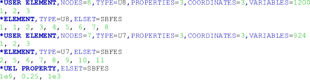
Figure 5: An example of ABAQUS input format involving SBFEM user elements

Figure 5 lists the definition used for the SBFEM user elements depicted in Fig. 4. With the keyword $\mathrm{\mathit{\mathrm{*USER\ ELEMENT}}}$, a new type of user element is declared. Then additional information regarding this element type, such as the number of nodes ($\mathrm{NODES}$), the type name ($\mathrm{TYPE}$), the number of property values ($\mathrm{PROPERTIES}$), the number of degrees of freedom (DOFs) per node ($\mathrm{COORDINATES}$), and the number of solution-dependent variables ($\mathrm{VARIABLES}$) are given. In the example, two user element types U8 and U7 are defined. In the next line, the DOFs per node are specified. In our examples, we use three-dimensional elements and therefore, each node has three translational DOFs. In ABAQUS, 1 denotes a displacement DOF in $x$-direction, while 2 and 3 represent the corresponding displacement DOFs in $y$- and $z$-directions, respectively. The definition of individual elements is similar to the standard format starting with the keyword $\mathrm{*ELEMENT}$. Here, only the element type that usually belongs to the standard ABAQUS element library is replaced by our user element type. The following line creates a single element by listing the element number and its nodes. The element property definition starts with the keyword $\mathrm{*UEL\ PROPERTY}$, then specifies the element set ($\mathrm{ELSET}$) it is assigned to. In the example, the element set is SBFES which includes Element 1 and Element 2 defined in the user element types U8 and U7, respectively. The property values are provided in the following line representing Young’s modulus, Poisson’s ratio and mass density. In our implementation, the solution-dependent variables contains static residual of the previous increment, static residual of the current increment, stiffness matrix, and mass matrix. Therefore for a user element with $n$ DOFs, the value of $\mathrm{VARIABLES}$ should be $n+n+n^{2}+n^{2}$.

Among the various definitions, two points deserve special mentions:

1. The SBFEM user element type is essentially determined by the number of nodes. For a two- or three-dimensional problem, the number of element nodes determines the number of DOFs of each element and further the dimensions of the output arrays of the $\mathrm{UEL}$. The SBFEM user elements having the same number of nodes can be classified as the same type, regardless of the element topology.

2. There is no requirement for the node ordering for one SBFEM user element, i.e., it can be arbitrary. For an ABAQUS built-in element, the node ordering should follow specific rules because it defines the topology of this element type. However, it is impossible to set a universal principle of describing the topology of the polyhedral element based only on the node ordering. The element topology will be described in a supplementary input text file introduced in Section 3.2.2. The node ordering of the SBFEM user element only affects the location vector for the assembly of the global stiffness matrix and force vector.

3.2.2 Text file format

As mentioned above, the ABAQUS input file only lists the node identifiers of each element, which is insufficient to describe the topology of polyhedral elements. Therefore, it is compulsory to provide additional information for the SBFEM user elements through a supplementary input file. There are four types of information in the supplementary file, shown in Fig. 6, i.e., (i) nodal coordinates, (ii) surface information, (iii) element information, and (iv) scaling center coordinates. At the beginning of each type of information, one integer is declared to identify the number of the specific entity such as nodes, surfaces, and elements. For each surface, one integer indicating the number of nodes is declared followed by the nodal connectivity of this surface, either clockwise or counter-clockwise. For the definition of a polyhedron, the number of surfaces is stated first, and then the identifiers of the surfaces enclosing the polyhedron are listed. The sign of surface ID is positive if the normal vector of the surface is pointing outward of the cell, otherwise it is negative.

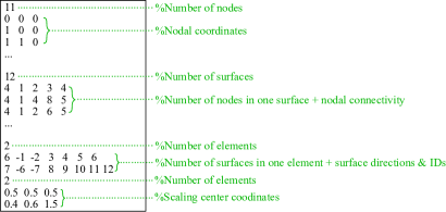
Figure 6: An example of text input format describing SBFEM polyhedral mesh

3.3 Data structure of the mesh information

The user subroutine $\mathrm{UEXTERNALDB}$ is the interface subroutine which allows communication between other programs and user subroutines within ABAQUS/Standard. In our implementation, it only plays a role at the beginning of the analysis. $\mathrm{UEXTERNALDB}$ reads the text file describing the SBFEM discretization and stores the mesh data into user-defined COMMON blocks. The mesh information allows the $\mathrm{UEL}$ to construct the element topology for defining the stiffness matrix $\mathbf{K}$, the mass matrix $\mathbf{M}$, etc.

Three COMMON blocks are created when the subroutine $\mathrm{UEXTERNALDB}$ is called. They are named as NDINFO, SFINFO and ELINFO, for storing the node, surface and element information, respectively. The explicit data structure of each block for the previous example is shown in Table 1.

Table 1: Data structure stored in the COMMON blocks

NDCRD
0.0	0.0	0.0
1.0	0.0	0.0
1.0	1.0	0.0
	$\cdots$

(a) Node information block NDINFO

SFCONN
1	2	3	4	1	4	8	5	1	2	6	$\cdots$
SFINDEX
4	8	12	16	20	24	28	31	34	38	41	44

(b) Surface information block SFINFO

ELCONN
-1	-2	3	4	5	6	-6	7	8	9	10	11	12
		ELINDEX					CTCRD
		6		13			0.5		0.5		0.5
							0.4		0.6		1.5

(c) Element information block ELINFO

The COMMON block NDINFO contains a matrix named NDCRD with dimension $n_{\mathrm{nd}}\times 3$ to store nodal coordinates, in which $n_{\mathrm{nd}}$ denotes the number of nodes.

The COMMON block SFINFO contains two vectors named SFCONN and SFINDEX, respectively. The vector SFCONN stores the nodal connectivity of each surface in a continuous fashion. An indexing vector SFINDEX is stored to recover the individual surface elements. It has $n_{\mathrm{sf}}$ entries, where $n_{\mathrm{sf}}$ represents the number of surfaces. Each entry of SFINDEX indicates the final storage position in SFCONN for each surface. The number of nodes for one surface can be calculated by the difference between the positioning entries of itself and the former surface. The first entry of SFINDEX is the number of nodes for the first surface as well.

The COMMON block ELINFO contains a vector named ELCONN, a vector named ELINDEX, and a matrix named CTCRD with dimension $n_{\mathrm{el}}\times 3$, where $n_{\mathrm{el}}$ is the number of elements. Similar to SFCONN, ELCONN stores the surfaces enclosing each element continuously, by the order of element ID. The indexing vector ELINDEX has $n_{\mathrm{el}}$ entries, which identify the final storage position of each element in ELCONN. The matrix CTCRD stores the scaling center coordinates of each element. For a subdomain without cracking, the scaling center may be calculated as the average coordinates of all nodes in each element. However, for cracked subdomain used in fracture mechanics, the scaling center should be specified as the crack tip [8]. To make the implementation more versatile, we purposely decided to provide the scaling center as additional input parameter.

The proposed scheme for storing polyhedral meshes is comparably memory-efficient. Only the matrices for storing coordinates, i.e., NDCRD and CTCRD, are provided as float data type while the components of other vectors are all integers. To minimize the memory requirements, we opted to store the surface and element information in vectors instead of matrices. Note that the number of nodes of each surface is not uniform and the polyhedral elements have arbitrary surfaces, which may induce zero entries in matrices. This issue can be avoided by using vectors to store the surface and mesh information.

3.4 User element

The user subroutine $\mathrm{UEL}$ is used to define a special element type not available in ABAQUS. It must provide all element level calculations, such as the definition of the stiffness and mass matrices as well as the residual force vector. To this end, ABAQUS provides some input variables to the $\mathrm{UEL}$, such as the current element number $\mathrm{JELEM}$, nodal coordinates $\mathrm{COORDS}$, material properties $\mathrm{PROPS}$, current nodal displacement vector U, and current solution procedure type $\mathrm{LFLAGS}$. Those variables are defined in the ABAQUS input file or generated automatically according to the simulation procedure. The most important arrays to output by the $\mathrm{UEL}$ are $\mathrm{AMATRX}$ and $\mathrm{RHS}$. For static analysis, $\mathrm{AMATRX}$ and $\mathrm{RHS}$ are the current stiffness matrix and residual force vector, respectively. In other analysis types, these generic arrays have different meanings. Detailed definitions of $\mathrm{AMATRX}$ and $\mathrm{RHS}$ for different solution procedures are out of the scope of the current section. The reader is referred to the ABAQUS user subroutine reference manual [35] for a comprehensive discussion.

The flowchart of the $\mathrm{UEL}$ subroutine implementing SBFEM is shown in Fig. 7. In the following, the functions and specific implementations of each process are explained in detail:

Figure 7: Flowchart of user subroutine UEL for SBFEM

1. Localization of nodal coordinates and construction of element topology: In this step, the global nodal coordinates are transformed into relative nodal coordinates with respect to the scaling center, and the element topology is constructed using local nodal identifiers. Two matrices named as RCRD and SELE are generated for storing the local nodal coordinates and the element topology, respectively. The global nodal coordinates ($x,y,z$) of the nodes belonging to the current element are passed into $\mathrm{UEL}$ as input matrix $\mathrm{COORDS}$. They are transformed into relative nodal coordinates ($\hat{x},\hat{y},\hat{z}$) with respect to the scaling center, which are used in Eq. (1). The sequence of the nodal coordinates conforms to the node ordering of each element given in the ABAQUS input file. The element topology can be extracted from the COMMON blocks when the element number $\mathrm{JELEM}$ is known. Note that the connectivity is given in terms of the global nodal identifiers. To meet the global assembly requirement, the calculation of $\mathrm{AMATRX}$ and $\mathrm{RHS}$ should match the node ordering given in the ABAQUS input file. Therefore, the element topology should be described using local nodal identifiers. Matching the nodal coordinates stored in $\mathrm{COORDS}$ and NDINFO, the correspondence between local and global nodal identifiers is obtained. Then, the element topology can be re-constructed by local nodal identifiers. During the construction of the element topology, the nodal connectivity of negative surfaces should be reordered for the mapping consideration. The RCRD and SELE for Element 2 (depicted in Fig. 4) are shown explicitly in Table 2, in which $n_{\mathrm{nd}}^{\mathrm{s}}$ represents the node number of each surface.

   Table 2: Data structures of relative nodal coordinates and element topology

   Global	Local
   5	1
   6	2
   7	3
   8	4
   9	5
   10	6
   11	7

   (a) Node ID correspondence

   $\hat{x}$	$\hat{y}$	$\hat{z}$
   -0.4	-0.6	-0.5
   0.6	-0.6	-0.5
   0.6	0.4	-0.5
   -0.4	0.4	-0.5
   -0.4	-0.6	0.5
   0.6	0.4	0.5
   -0.4	0.4	0.5

   (b) RCRD

   $n_{\mathrm{nd}}^{\mathrm{s}}$	Local nodal connectivity
   4	4	3	2	1
   4	5	7	4	1
   3	1	2	5	0
   3	2	3	6	0
   4	3	4	7	6
   3	2	6	5	0
   3	5	6	7	0

   (c) SELE

2. Calculation of the elasticity matrix $\mathbf{D}$: The material properties such as Young’s modulus, Poisson’s ratio and mass density are stored in the input array named PROPS. Using Young’s modulus and Poisson’s ratio, the elasticity matrix $\mathbf{D}$ can be formulated as in Eq. (13).

3. Preparation of matrices $\mathbf{N_{\mathrm{u}}}$, $\mathbf{J}_{\mathrm{b}}$, $\mathbf{B}_{1}$ and $\mathbf{B}_{2}$: The shape function matrix $\mathbf{N_{\mathrm{u}}}$ depends on the surface element type, which can be either a triangular or quadrilateral element, with linear or quadratic shape functions. The surface element type has been defined in the matrix SELE generated in the previous step. Extracting the nodal coordinate vectors $\mathbf{x}$, $\mathbf{y}$, and $\mathbf{z}$ of the surface from the matrix RCRD, together with the shape function matrix $\mathbf{N}_{\mathrm{u}}$, the Jacobian matrix $\mathbf{J}_{\mathrm{b}}$ is formulated following Eqs. (1) and (3). After computing the matrices $\mathbf{b}_{1}$, $\mathbf{b}_{2}$ and $\mathbf{b}_{3}$ based on $\mathbf{J}_{\mathrm{b}}^{-1}$, the matrices $\mathbf{B}_{1}$ and $\mathbf{B}_{2}$ are calculated by Eq. (11).

4. Integration of $\mathbf{E}_{0}^{\mathrm{e}}$, $\mathbf{E}_{1}^{\mathrm{e}}$, $\mathbf{E}_{2}^{\mathrm{e}}$ and $\mathbf{M}_{0}^{\mathrm{e}}$: The integrals to determine the coefficient matrices of the individual surface elements, see Eq. (15), are solved using numerical quadrature rules, in our case, a standard Gaussian quadrature rule. Then the coefficient matrices $\mathbf{E}_{0}$, $\mathbf{E}_{1}$, $\mathbf{E}_{2}$ and $\mathbf{M}_{0}$ of the entire element are assembled from the coefficient matrices $\mathbf{E}_{0}^{\mathrm{e}}$, $\mathbf{E}_{1}^{\mathrm{e}}$, $\mathbf{E}_{2}^{\mathrm{e}}$ and $\mathbf{M}_{0}^{\mathrm{e}}$ of all surface elements.

5. Calculation and eigenvalue decomposition of $\mathbf{Z}_{\mathrm{p}}$: The expression of the coefficient matrix $\mathbf{Z}_{\mathrm{p}}$ is provided in Eq. (19), which can be computed based on $\mathbf{E}_{0}$, $\mathbf{E}_{1}$, $\mathbf{E}_{2}$ and $\mathbf{E}_{0}^{-1}$. For computing the inverse of $\mathbf{E}_{0}$, two subroutines DGETRF and DGETRS from the Linear Algebra PACKage (LAPACK) [56] are called. DGETRF prepares the LU factorization of $\mathbf{E}_{0}$ for DGETRS to compute $\mathbf{E}_{0}^{-1}$. The eigenvalue decomposition of $\mathbf{Z}_{\mathrm{p}}$ is implemented by calling the subroutine DGEEV of LAPACK. DGEEV provides a matrix and two vectors as output parameters. The matrix alternately stores the real and imaginary parts of the right eigenvectors in its columns. The two vectors store the real and imaginary parts of eigenvalues, respectively. They are essentially the eigenvector matrix and eigenvalues in Eq. (20), but in the DGEEV output format. The real parts of eigenvalues are sorted by the descending order through bubble sort algorithm [57]. The imaginary parts of eigenvalues and eigenvectors are sorted also following the sorted real parts of the eigenvalues. Combining real parts and imaginary parts, the eigenvector matrix $\mathbf{\Phi}$ and the diagonal matrix of eigenvalues $\mathbf{\Lambda}$ given in Eq. (22) are obtained. They are complex matrices and stored with double complex data type. The sub-matrices $\mathbf{\Phi}_{\mathrm{u1}}$, $\mathbf{\Phi}_{\mathrm{q1}}$ and $\mathbf{\Lambda}^{+}$ can be extracted easily from $\mathbf{\Phi}$ and $\mathbf{\Lambda}$.

6. Formulation and storage of $\mathbf{K}$ and $\mathbf{M}$: The stiffness matrix $\mathbf{K}$ can be calculated by Eq. (26), in which the calculation of the inverse of sub-matrices $\mathbf{\Phi}_{\mathrm{u1}}$ can be done analogously to the inversion of $\mathbf{E}_{0}$ discussed in Step 5. The mass matrix $\mathbf{M}$ is computed step by step through implementing the Eqs. (27)–(31). At the end of the first increment of an analysis, the stiffness and mass matrices are stored in the array $\mathrm{SVARS}$ of the $\mathrm{UEL}$ for later use.

7. Definition of $\mathrm{AMATRX}$ and $\mathrm{RHS}$: Generally speaking, for all types of solution procedure related to solid mechanics, we can defined the output arrays $\mathrm{AMATRX}$ and $\mathrm{RHS}$ based on the existing calculated arrays and input arrays. $\mathrm{AMATRX}$ is always defined as stiffness matrix $\mathbf{K}$, mass matrix $\mathbf{M}$, damping matrix $\mathbf{C}$ or a combination thereof obeying specific rules. The damping matrix $\mathbf{C}$ of a linear user element can be defined by Rayleigh damping [35]

   $$\mathbf{C}=\alpha\mathbf{M}+\beta\mathbf{K},$$ (32)

   where $\alpha$ and $\beta$ are the user-specified Rayleigh damping factors. $\mathrm{RHS}$ is always defined through the internal force vector or its combination with the inertia force vector obeying specific rules. The internal force vector can be obtained by

   $$\mathrm{\mathbf{F}_{S}=\mathbf{KU}},$$ (33)

   where $\mathbf{U}$ is the current nodal displacement vector, one input array of the $\mathrm{UEL}$. For linear static problem, $\mathrm{RHS}$ is formulated as $-\mathbf{F}_{\mathrm{S}}$. The inertia force vector can be calculated as

   $$\mathrm{\mathbf{F}_{I}=\mathbf{MA}}.$$ (34)

   $\mathbf{A}$ is the current nodal acceleration vector, and it is also one input array of the $\mathrm{UEL}$. The inertia force vector $\mathbf{F}_{\mathrm{I}}$ contributes to $\mathrm{RHS}$ in dynamic problems.

8. Reading of matrices ($\mathbf{K}$, $\mathbf{M}$) stored in Step 6: For the increments except for the first one, the stiffness and mass matrices are retrieved directly from the array $\mathrm{SVARS}$.

3.5 Element-based surface definition

The element-based surface definition for the SBFEM user element is important to take advantage of different features inherent to ABAQUS. By defining an element-based surface, distributed loads such as pressure and surface traction can be assigned to that surface. More importantly, for interfacial problems involving interactions such as tie constraints or contact definitions, it is a prerequisite to define surfaces to establish these interactions.

Currently, element-based surfaces can be created on solid, continuum shell, and cohesive elements in ABAQUS. On user elements, only node-based surfaces can be created, and they act only as slave surfaces and always use node-to-surface schemes in contact analysis, which is a severe shortcoming as the node-to-surface contact may fail the contact patch test even for a flat interface [14].

By overlaying standard elements with nearly zero stiffness on the SBFEM user elements, it is possible to define element-based surfaces for the SBFEM user elements. In the numerical examples, presented in the following section, the Young’s modulus of the overlaid elements is chosen in accordance with the value of the adjacent user element and scaled accordingly, i.e., $E_{\mathrm{ov}}=10^{-16}E_{\mathrm{UEL}}$. This methodology has originally been proposed in the ABAQUS manual [35] to visualize the user elements and is modified in this contribution to define element-based surfaces. The modification is related to the fact that instead of overlaying the entire polyhedral element with the standard finite elements only the volume sector needed for the surface definition are included. The volume sectors of the three-dimensional SBFEM user elements are either of tetrahedral or pyramidal shape depending on the corresponding surface element type, i.e., either triangular or quadrilateral. Those shapes can be easily overlaid by standard elements from ABAQUS’ element library. As the scaling center fulfills the star-convexity requirement, i.e., the entire boundary is directly visible from this point, the process of creating this overlay mesh is robust for all types of polyhedrons. Hence, the element-based surfaces can be directly created on the overlaid standard elements as they share the DOFs with the corresponding SBFEM user elements. Note that this methodology does not affect the solution quality as the overlay elements contribute a negligible stiffness to the global system. Considering the shape functions on the surface of the SBFEM user elements it must be stressed again that they coincide with those of the elements from ABAQUS’ element library.

The operation of overlaying standard elements on the volume sectors of the SBFEM user element is illustrated in Fig. 8. This particular example is based on the SBFEM user element depicted in Fig. 8a which consists of six surfaces and eight nodes. Note that the scaling center is marked in red (Node 9). Here, a quadrilateral element-based surface is created by introducing a pyramidal overlay element that is superimposed on the volume sector created be surface element S1 and the scaling center. This procedure is straightforward as ABAQUS offers pyramidal finite elements such as the C3D5 element. The ABAQUS input file format for defining this element-based surface is given in Fig. 8b. It is important to keep in mind that in our implementation, the scaling center is not an actual node of the element and consequently, must be defined in the ABAQUS input file. The surface identifier S1 indicates the surface formed by the first four nodes of the pyramidal element [35]. If a triangular element-based surface is to be created, the corresponding volume sector must be superimposed by a standard tetrahedral element, e.g., the C3D4 element.

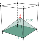
(a) Overlaying operation

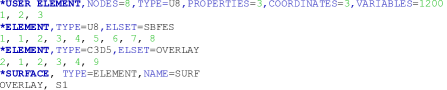
(b) Input format

Figure 8: Overlaying standard element on SBFEM user element for defining surface

4 Numerical examples

The objective of this section is to verify the implementation and demonstrate the advantages of including SBFEM user elements. This is achieved by means of various numerical examples. In the first subsection, benchmark tests are performed to check the correct implementation. The second subsection presents examples considering the treatment of non-matching meshes. The third subsection includes examples that are related to automatically generated meshes based on image and STL data. In these cases, robust and efficient octree mesh generation algorithms are employed. The computational times reported are measured on a DELL workstation with an Intel Xeon E5-2637 CPU running Windows 10 Pro, 64 bit.

4.1 Benchmark tests

This subsection is designated to verify the implementation of SBFEM user elements by performing static, modal, and transient analyses on simple geometries. A patch test is performed on a quadrangular prism under uniaxial tension in order to check the implementation of the stiffness matrix. Modal and transient analyses are performed on a cantilever beam to verify the implementation of the mass matrix.

4.1.1 Patch test

A quadrangular prism is discretized by five polyhedral elements as shown in Fig. 9. The dimensions are indicated in Fig. 9 with $b=h=1\,\mathrm{m}$. The material constants are Young’s modulus $E=10\,\mathrm{GPa}$ and Poisson’s ratio $\nu=0.25$. The left surface (nodes with $x=0$) of the quadrangular prism is constrained in $x$-direction, the front surface (nodes with $y=0$) is constrained in $y$-direction, and the bottom surface (nodes with $z=0$) is constrained in $z$-direction. A vertical force $F=1000\,\mathrm{kN}$ is applied at Nodes 19, 20, 21 and 22 on the top surface.

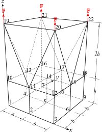
Figure 9: Modeling of a quadrangular prism

The theoretical solutions of displacement $u_{z}$ and stress $\sigma_{z}$ of the uniaxial tension problem are expressed as:

$$\sigma_{z}=\frac{F}{b^{2}}=1\,\mathrm{MPa},$$ (35a)

$$u_{z}=\left(\frac{\sigma_{z}}{E}-\frac{\nu\sigma_{x}}{E}-\frac{\nu\sigma_{y}}{E}\right)z=\frac{F}{Eb^{2}}z=0.0001z.$$ (35b)

The corresponding contours are depicted in Fig. 10. The maximum nodal $L^{2}$ error norms of displacement $u_{z}$ and stress $\sigma_{z}$, which are calculated based on the analytical solutions in Eq. (35), are listed in Table 3. The displacement and stress results are considered to be accurate up to the machine precision.

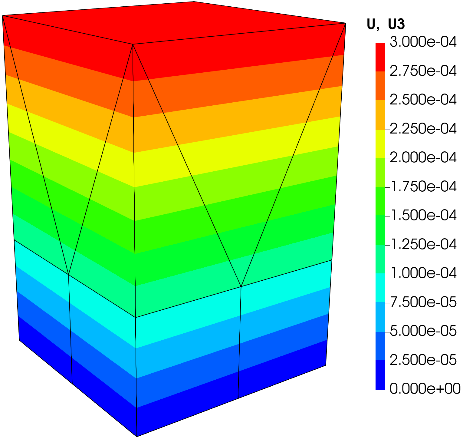
(a) Displacement contour $u_{z}$ (Unit: m)

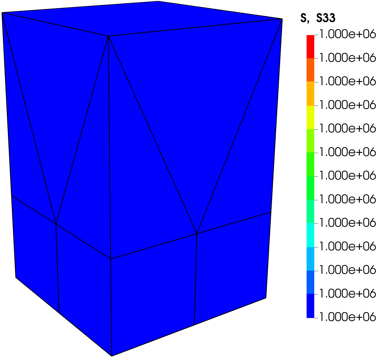
(b) Stress contour $\sigma_{z}$ (Unit: Pa)

Figure 10: Contours of a quadrangular prism under uniaxial tension

Table 3: Maximum nodal $L^{2}$ error norm of a quadrangular prism under uniaxial tension

	$u_{z}$	$\sigma_{z}$
$L^{2}$ error norm	1.199e-14	1.695e-14

4.1.2 Modal analysis of a cantilever beam

The second example is a three-dimensional cantilever beam with a depth of $d=0.4\,\mathrm{m}$, a thickness of $t=0.2\,\mathrm{m}$, and a length of $l=1\,\mathrm{m}$, where one end of the beam is clamped, as shown in Fig. 11a. The material properties are Young’s modulus $E=1\,\mathrm{MPa}$, Poisson’s ratio $\nu=0.25$, and the mass density $\rho=2000\,\mathrm{kg/m^{3}}$.

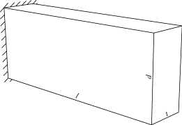
(a) Geometry and boundary condition

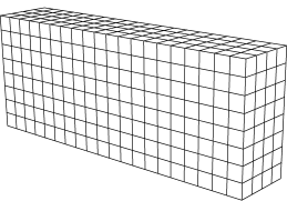
(b) Mesh

Figure 11: Model of a cantilever beam

Three-dimensional SBFEM user elements and 8-node linear brick elements (ABAQUS: C3D8) are assigned to the same mesh to compare their performances. In the following, we refer to the mesh assigned with ABAQUS library’s elements as ABAQUS model and the mesh assigned with SBFEM user elements as SBFEM model. Four meshes of the cantilever beam with different element sizes, i.e., $0.1\,\mathrm{m}$, $0.05\,\mathrm{m}$, $0.025\,\mathrm{m}$ and $0.0125\,\mathrm{m}$, are generated and one is shown in Fig. 11b (mesh size: $0.05\,\mathrm{m}$). The reference model has a mesh size of $0.004\,\mathrm{m}$, consisting of 1,250,000 C3D8 elements and 1,292,901 nodes.

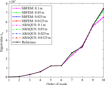
(a) First 10 eigenvalues

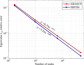
(b) Convergence of eigenvalue $\lambda_{10}$

Figure 12: Modal analysis comparison of a cantilever beam

For all models, an eigenvalue analysis is performed using the default settings of ABAQUS’ solver [35]. The first ten eigenvalues for the different models are plotted in Fig. 12a. As can be observed, the first ten eigenvalues converge algebraically for both element types. The convergence in the relative error norm of eigenvalue $\lambda_{10}$ is also studied. The relative error of eigenvalue $\lambda_{10}$ is determined by $E_{\mathrm{rel}}=(\lambda_{10}-\lambda_{10}^{\mathrm{ref}})$/$\lambda_{10}^{\mathrm{ref}}$, where $\lambda_{10}^{\mathrm{ref}}$ is the 10th eigenvalue obtained from the reference model. The relative errors versus the number of nodes for the two types of models are plotted in Fig. 12b. The results are in good agreement, while the SBFEM models achieve slightly more accurate results.

4.1.3 Transient analysis of a cantilever beam

A transient analysis is performed on the three-dimensional cantilever beam structure introduced in the previous section. The boundary conditions and load history are shown in Fig. 13. A distributed line load $q(t)=2\sin(2\pi t)$ (Unit: $\mathrm{kN/m}$) acting on the top edge of the free end varies harmonically in time for $2.5\,\mathrm{s}$, as depicted in Fig. 13b. As a monitor point, we choose the middle point on the lower edge of the free end of the cantilever beam as indicated in Fig. 13a. The vertical responses of the monitor point are recorded.

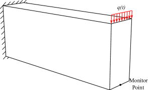
(a) Boundary and load conditions

(b) Load history

Figure 13: A cantilever beam subjected to dynamic loading

The responses of the SBFEM and ABAQUS reference models are compared. The mesh size of the SBFEM model is chosen as $0.025\,\mathrm{m}$ which is related to the modal analysis results. It has been shown that the first ten eigenvalues are accurately captured by this model (error less than $1\%$). The reference model is identical to the one used in the previous section. The time stepping method is the Hilber-Hughes-Taylor (HHT) method [58] implemented in ABAQUS/Standard, which is an unconditionally stable method for linear problems. Again, the default settings for the transient (implicit dynamic) analysis [35] have been employed. A maximum time step size of $0.01\,\mathrm{s}$ has been chosen and the automatic time stepping of ABAQUS is activated. The vertical responses at the monitor point during the $2.5\,\mathrm{s}$ simulation time are obtained from the two models and plotted in Fig. 14. An excellent agreement is found as the difference between the results obtained from the SBFEM and ABAQUS reference models is negligible. Only in the acceleration response during the first $0.5\,\mathrm{s}$ small deviations are visible.

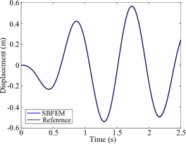
(a) Displacement

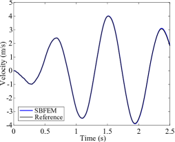
(b) Velocity

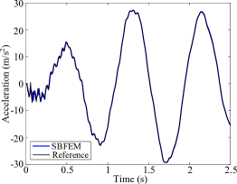
(c) Acceleration

Figure 14: Response history of a 3D cantilever beam: vertical response at monitor point

4.2 Examples for non-matching meshes

Non-matching meshes often occur in finite element analyses involving domain decomposition [31, 59] and contact mechanics [14] problems. Typically, special techniques are required to enforce the compatibility and equilibrium at the interfaces of non-matching meshes, which often introduce additional unknowns. Non-matching meshes in the finite element sense can be easily converted to matching meshes owing to flexibility provided by polyhedral SBFEM domains, which allows for elements with an arbitrary number of faces.

This section presents three examples to demonstrate the advantages of the matching meshes. The first example investigates the performance of the proposed elements in contact patch tests having curved interfaces. In the second example, a patch test including cohesive elements in conjunction with contact is presented. This example highlights the convenience of inserting cohesive elements at matching interfaces and verifies the behavior of cohesive elements combined with SBFEM user elements. The third example presents a cube with a spherical inclusion. Here, interaction states containing both contact and traction are examined and compared with the results obtained from non-matching meshes.

4.2.1 Patch test for contact analysis

ABAQUS/Standard provides comprehensive approaches for defining contact interactions: general contact, contact pairs and contact elements. For these approaches, there are different formulations available such as node-to-surface (NTS), or surface-to-surface (STS) techniques which are available for contact pairs [35]. Although many approaches can be utilized, the non-uniformity of the contact interface discretization may reduce the accuracy of results in ABAQUS [14, 13]. The performance of contact models in ABAQUS is expected to be enhanced when matching contact interfaces can be easily generated.

Three-dimensional contact patch tests are studied for the most commonly used NTS and STS schemes. The model is illustrated in Fig. 15 with dimensions defined as $W=6\,\mathrm{m}$ and $h=3\,\mathrm{m}$. It features a spherical contact interface between two blocks with a maximum deviation distance $d$. The shape of the interface is described as

$$z_{\mathrm{i}}(x_{\mathrm{i}},y_{\mathrm{i}})=d\left[1-\frac{2\left(x_{\mathrm{i}}^{2}+y_{\mathrm{i}}^{2}\right)}{W^{2}}\right],$$ (36)

where $x_{\mathrm{i}}$, $y_{\mathrm{i}}$, $z_{\mathrm{i}}$ are the coordinates of a point on the interface. The parameter $d$ varies from $0$ to $1.5\,\mathrm{m}$ to examine the contact performance depending on the actual shape of the curved contact interface. The model has a Young’s modulus of $E=10\,\mathrm{MPa}$, and a Poisson’s ratio of $\nu=0.3$. The contact has a friction coefficient of $\mu=0.5$. The lower interface is selected as the master surface of the contact. Six degrees of freedom of the lower block (as indicated in Fig. 15) are fixed to prevent rigid body motions. A uniform pressure $P=1\,\mathrm{MPa}$ is applied at the bottom and top surfaces and consequently, a constant stress state $\sigma_{z}=1\,\mathrm{MPa}$ is expected in the contact patch test.

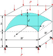
(a) Model

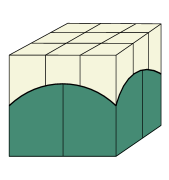
(b) Mesh scheme

Figure 15: Patch test model for contact analysis

The basic set-up of the discretization for the model is shown in Fig. 15b, where it is observed that the top and bottom contact bodies are divided into nine and four elements, respectively. C3D8 elements are assigned to the non-matching meshes directly, as shown in Fig. 16a. The special treatment ’slave tolerance’ in ABAQUS is used to detect the effective contact pairs for the ABAQUS models due to initial gaps or penetrations. Through re-meshing the interface, the hexahedral non-matching meshes are converted to polyhedral matching meshes as illustrated in Fig. 16b. The SBFEM user elements can be directly assigned to the matching meshes (see Fig. 16b) as they allow polyhedral shapes. Element-based surfaces can be created for the SBFEM models through the methodology proposed in Section 3.5, which are used to establish the contact pairs.

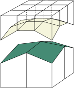
(a) Non-matching mesh

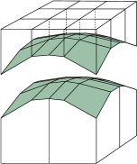
(b) Matching mesh

Figure 16: Meshes of contact patch test

The stress contours of $\sigma_{z}$ (S33), obtained from the ABAQUS and SBFEM models (STS) are plotted in Figs. 17 and 18, respectively. The relative $L^{2}$ error norms for $\sigma_{z}$ are listed in Table 4, in which the maximum error norms of nodal stress are given. As shown in Fig. 17 and Table 4, for the ABAQUS models applying the STS scheme, only the model with flat contact interface obtains accurate result and passes the patch test. By increasing the curvature of the contact surfaces, the accuracy of the ABAQUS models deteriorates. This effect is attributed to initial gaps or penetrations in non-matching interface meshes which reduce the accuracy of the contact simulation. All ABAQUS models applying the NTS scheme fail the patch tests with substantial errors. In contrast, the SBFEM models provide accurate results (up to machine precision) and pass the patch tests for various curvatures using both STS and NTS schemes, as depicted in Fig. 18 and Table 4.

Table 4: $L^{2}$ Error norm of $\sigma_{z}$ of different models with different curvatures

		$d=0$	$d=0.5\,\mathrm{m}$	$d=1\,\mathrm{m}$	$d=1.5\,\mathrm{m}$
STS	ABAQUS model	<1e-9	3.72e-3	1.31e-2	2.72e-1
	SBFEM model	4.77e-14	4.10e-14	6.48e-14	5.02e-14
NTS	ABAQUS model	1.24e-1	1.16e-1	1.12e-1	1.11e-1
	SBFEM model	5.13e-14	5.24e-14	6.76e-14	6.17e-14

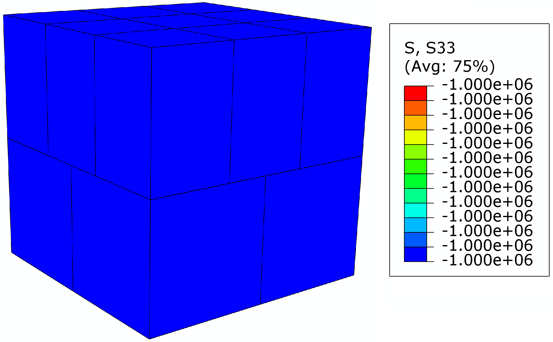
(a) $d$=0m

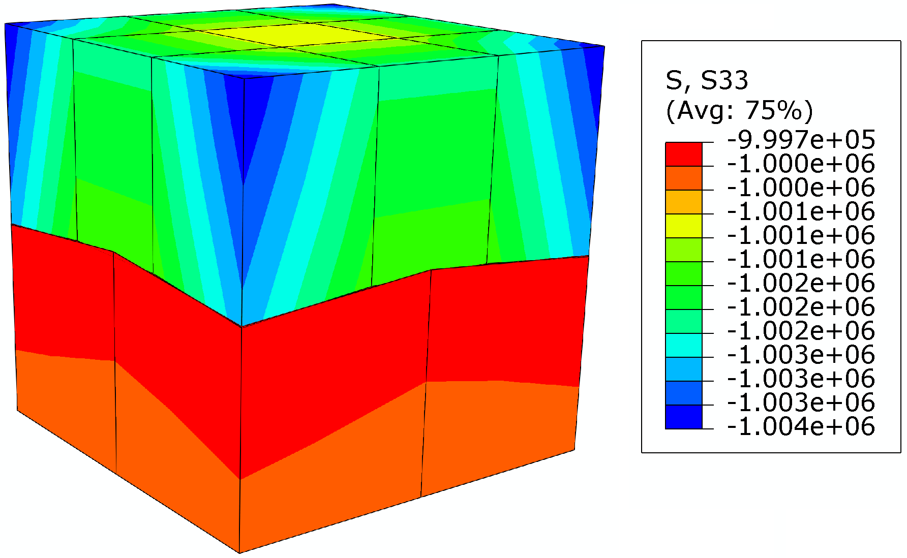
(b) $d$=0.5m

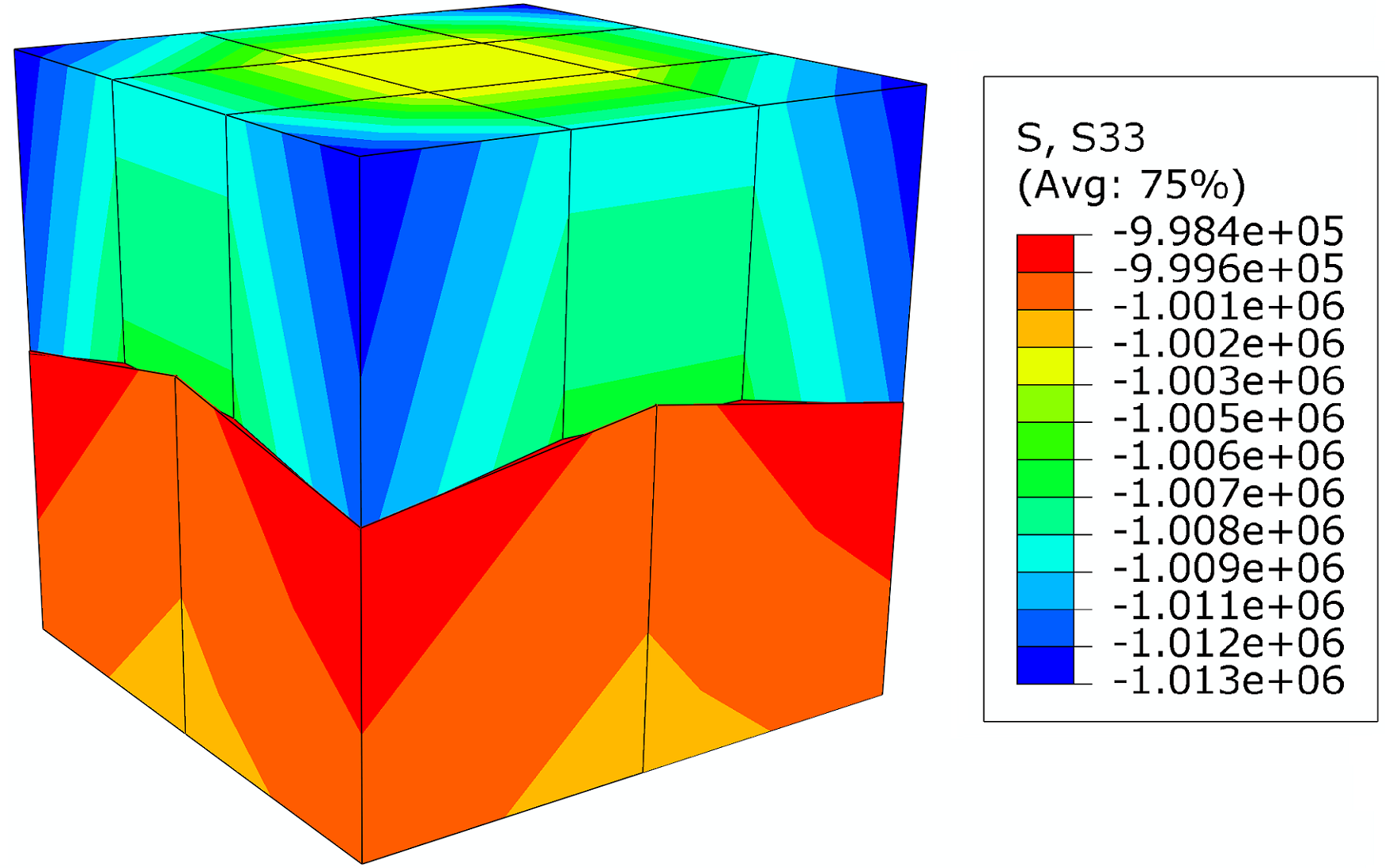
(c) $d$=1m

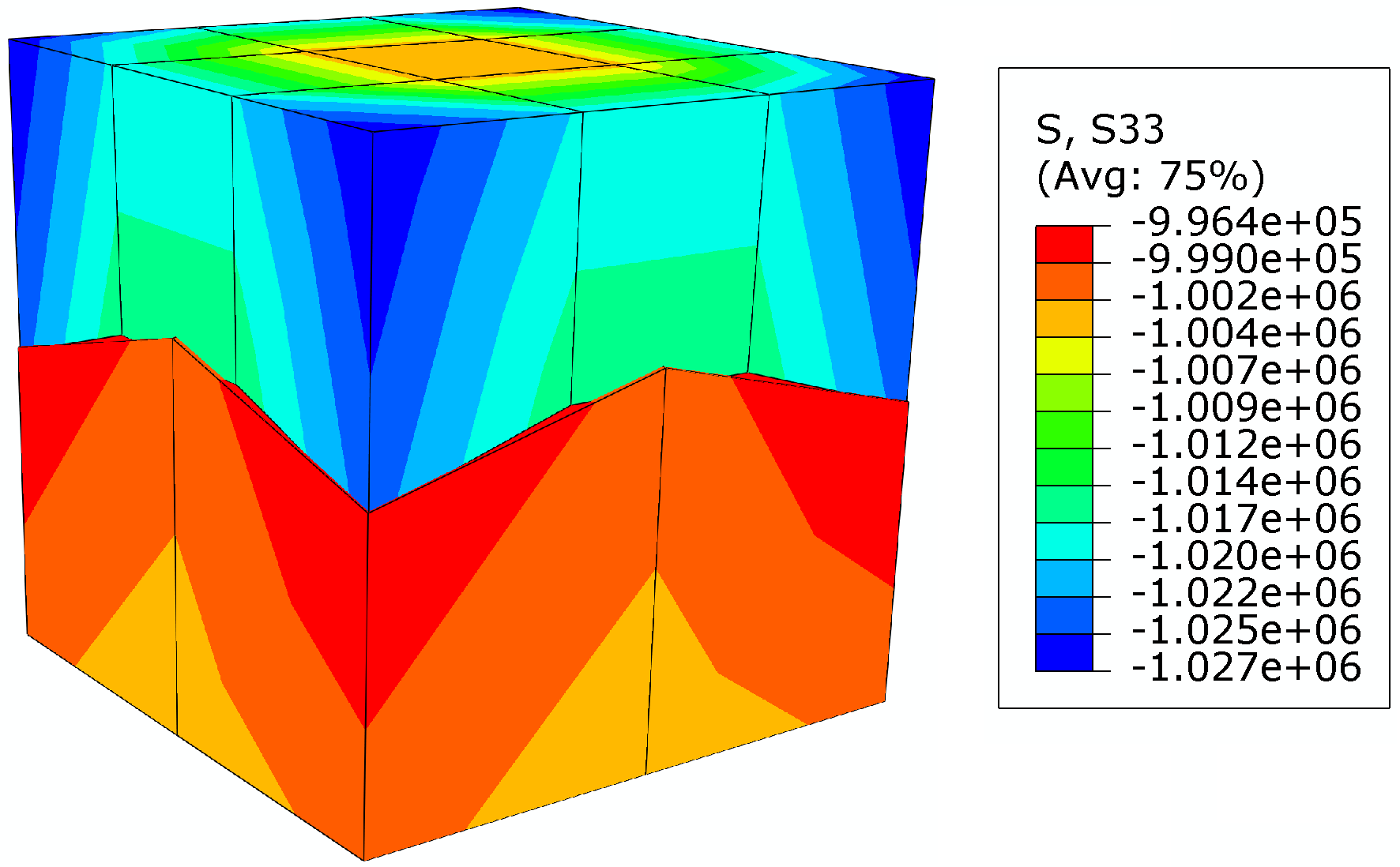
(d) $d$=1.5m

Figure 17: Stress contours ($\sigma_{z}$) of ABAQUS models (Unit: Pa)

(a) $d$=0m

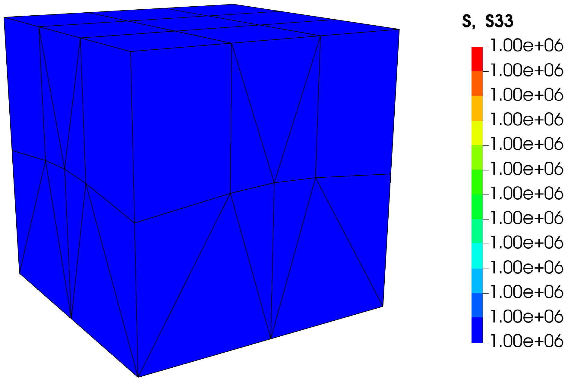
(b) $d$=0.5m

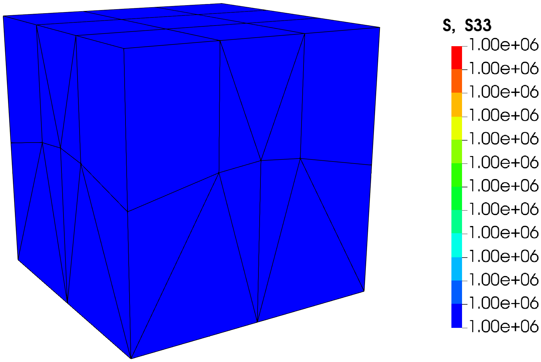
(c) $d$=1m

(d) $d$=1.5m

Figure 18: Stress contours ($\sigma_{z}$) of SBFEM models (Unit: Pa)

4.2.2 Patch test of cohesive element in conjunction with contact

In composite materials, such as concrete [60] and fiber-reinforced plastics [59], interfacial stresses between the bulk materials develop when they separate. To investigate the behavior of the interfacial transition zone (ITZ), cohesive elements are widely used in literature [61, 62, 63]. The geometry of the microstructure and the interface conditions have a significant influence on the macroscopic behavior of composite materials [64]. Therefore, surface meshes located at the material interface should provide a highly accurate representation of the actual geometry being suitable for simulating the interactions. Matching meshes, which are easily obtained from polyhedral elements, eliminate the gaps and penetrations at the interface and two matching surfaces can directly form a cohesive element. The performance of the combination of existing cohesive elements in ABAQUS and the proposed user elements is investigated in the following.

The scheme of the numerical modeling for the ITZ based on the matching meshes is illustrated in Fig. 19. There are two hexahedral domains representing the bulk materials, and they exhibit a matching discretization at the interface. For the sake of clarity, the matching meshes in Fig. 19 have been separated, while essentially they are exactly matching with no gap, i.e., Nodes 5 and 9 have the same coordinates, which is also true for the other matching nodes. These two surfaces can straightforwardly form a zero thickness cohesive element. An 8-node three-dimensional cohesive element COH3D8 can be defined with node ordering ’5, 6, 7, 8, 9, 10, 11, 12’. In this way, no constraints are required to connect the cohesive element to the other components. To prevent the interpenetration, a contact pair is established based on the two surfaces of the two blocks. The cohesive element generates traction applied to the surrounding bulk materials when they separate. The contact pair will be activated when interpenetration between bulk materials might occur. For triangular matching interfaces, a 6-node three-dimensional cohesive element COH3D6 must be used.

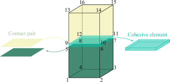
Figure 19: Numerical modeling of ITZ

For a better understanding, the basic description of the the constitutive response of cohesive elements using a traction-separation law is provided. Readers interested in a comprehensive discussion should refer to the ABAQUS manual [35]. Cohesive elements typically employ a traction-separation response in the normal direction based on an exponential damage evolution law which is depicted in Fig. 20. The traction-separation response in tension contains a damage evolution described by a scalar damage value $D$, and can be expressed as

$$t_{n}=\begin{cases}E_{n}\delta_{n}&\delta_{n}^{\mathrm{max}}\leq\delta_{n}^{\mathrm{o}}\\ \left(1-D\right)E_{n}\delta_{n}&\delta_{n}^{\mathrm{o}}<\delta_{n}^{\mathrm{max}}\leq\delta_{n}^{\mathrm{f}}\\ 0&\delta_{n}^{\mathrm{max}}>\delta_{n}^{\mathrm{f}}\end{cases},$$ (37)

where $t_{n}$ and $\delta_{n}$ represent the traction and separation, and $E_{n}$ is the initial elastic modulus of the cohesive element in the normal direction. The parameters $\delta_{n}^{\mathrm{o}}$, $\delta_{n}^{\mathrm{f}}$, $\delta_{n}^{\mathrm{max}}$ represent the separation at different states, they indicate damage initiation, complete failure, and the maximum value attained during loading, respectively. The damage variable, $D$, represents the overall damage of the cohesive element. It has an initial value of 0 before damage initiation and then monotonically evolves from 0 to 1 until total damage occurs. For an exponential softening law, when $\delta_{n}^{\mathrm{o}}<\delta_{n}^{\mathrm{max}}<\delta_{n}^{\mathrm{f}}$, the damage variable $D$ is expressed as

$$D=1-\left(\frac{\delta_{n}^{\mathrm{o}}}{\delta_{n}^{\mathrm{max}}}\right)\left\{1-\frac{1-\exp\left[-\alpha\left(\frac{\delta_{n}^{\mathrm{max}}-\delta_{n}^{\mathrm{o}}}{\delta_{n}^{\mathrm{f}}-\delta_{n}^{\mathrm{o}}}\right)\right]}{1-\exp(-\alpha)}\right\},$$ (38)

where $\alpha$ is the exponential coefficient. The cohesive element will not be damaged if it is in compression, thus the response in Fig. 20 is straight when $\delta_{n}<0$.

Figure 20: Typical traction-separation response with exponential damage evolution

To assess the compatibility of SBFEM user elements and cohesive elements, we use the same mesh that was already used for the contact investigations, i.e., a simple hexahedral domains with a flat interface, and insert cohesive elements at the interface. As shown in Fig. 21, zero thickness cohesive elements are generated at the matching interface. In addition, the contact pairs are established on the matching surfaces for preventing the interpenetration of the two parts. The bottom of the lower block is constrained in the vertical direction, and three DOFs are fixed in the horizontal directions to prevent rigid body motions.

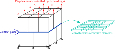
Figure 21: Patch test model with cohesive element

The material properties used in this example are listed in Table 5. The material properties of the cohesive elements are chosen for the purpose of the verification, they do not represent any specific mechanical behavior. The tangential properties of the cohesive elements are not listed because the patch test only generates normal stresses. The SBFEM elements are relatively rigid, such that the displacement load $d$ will be mainly transferred to $\delta_{n}$ when it is positive. When the cohesive elements have no damage ($\delta_{n}^{\mathrm{max}}\leq\delta_{n}^{\mathrm{o}}$), the ratio between $\delta_{n}$ and $d$ is 0.99997 for $d>0$ based on elasticity theory, and it will increase if the damage initiation occurs in the cohesive elements.

Table 5: Material properties of the patch test inserting cohesive element

	Young’s modulus $E\left[\mathrm{MPa}\right]$	Poisson’s ratio $\nu$	$\delta_{m}^{\mathrm{o}}\left[\mathrm{m}\right]$	$\delta_{m}^{\mathrm{f}}\left[\mathrm{m}\right]$	$\alpha$
Cohesive	$1$	-	$0.001$	$0.005$	2
Bulk	$200000$	0.3	-	-	-

A static analysis is performed to observe the behavior of the cohesive elements. Three harmonically varying cyclic displacement-controlled loads $d$ are applied on the top surface of the upper block, as plotted in Fig. 22a. The expression of $d$ (Unit: $\mathrm{mm}$) in terms of time $t(\mathrm{s})$ is

$$d=\begin{cases}0.8\sin 2\pi t&0\leq t\leq 1\\ 2\sin 2\pi(t-1)&1<t\leq 2\\ 6\sin 2\pi(t-2)&2<t\leq 3\end{cases}.$$ (39)

The magnitudes of $d$ are chosen to generate different $\delta_{n}^{\mathrm{max}}$ representing different damage states in the three cycles. In the first cycle ($0\leq t\leq 1\,\mathrm{s}$), the harmonic loading generates a $\delta_{n}^{\mathrm{max}}=0.08\,\mathrm{mm}<\delta_{n}^{\mathrm{o}}$, which indicates there is no damage in the cohesive elements. The second cycle ($1\,\mathrm{s}<t\leq 2\,\mathrm{s}$) has a $\delta_{n}^{\mathrm{max}}=2\,\mathrm{mm}$ which satisfies $\delta_{n}^{\mathrm{o}}<\delta_{n}^{\mathrm{max}}<\delta_{n}^{\mathrm{f}}$, and the cohesive elements are partially damaged in this stage. The third cycle ($2\,\mathrm{s}<t\leq 3\,\mathrm{s}$) will cause complete failure of the cohesive elements, since it results in $\delta_{n}^{\mathrm{max}}=6\,\mathrm{mm}>\delta_{n}^{\mathrm{f}}$.

The numerical result for the history of $\delta_{n}$ in the three cycles is plotted in Fig. 22a. During the loading history, the normal separation $\delta_{n}$ has the following results:

$$\delta_{n}\begin{cases}\approx d&d\geqslant 0\\ =0&d<0\end{cases}.$$ (40)

When $d\geqslant 0$, $\delta_{n}$ is quite similar to $d$ with negligible distinction as explained before. If $d<0$, $\delta_{n}$ equals to 0 because the surfaces of cohesive elements share the same DOFs with the contact surfaces of the two blocks, while the interpenetration between them is prevented by the contact pairs.

The evolution of the normal traction $t_{n}$ versus $\delta_{n}$ is depicted in Fig. 22b. Some feature points are plotted in Fig. 22 to clarify the behavior of cohesive elements during different loading cycles. During unloading, the normal traction $t_{n}$ always varies linearly and goes back to the origin. The response of the normal traction $t_{n}$ during loading in the three cycles is described as follows:

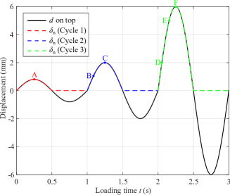
(a) Displacement history

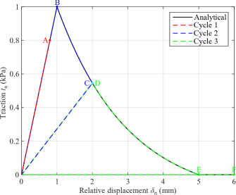
(b) Normal stress evolution

Figure 22: Cohesive element behavior under cyclic loading (with contact)

1. In Cycle 1, $t_{n}$ varies linearly according to $\delta_{n}$ following $t_{n}=E_{n}\delta_{n}$. It reaches its peak value $0.8\,\mathrm{kPa}$ at Point A and then decreases to 0, after which it remains 0.

2. In Cycle 2, the initial relationship between $t_{n}$ and $\delta_{n}$ is $t_{n}=E_{n}\delta_{n}$ until $\delta_{n}$ increases to $\delta_{n}^{\mathrm{o}}$ (Point B), where the damage initiation occurs and $t_{n}$ reaches its peak value $1\,\mathrm{kPa}$. After Point B, $t_{n}$ decreases with the increase of $\delta_{n}$ to $0.54\,\mathrm{kPa}$ (Point C), following the analytical damage evolution law. At Point C, $\delta_{n}$ reaches its current $\delta_{n}^{\mathrm{max}}$ which is between $\delta_{n}^{\mathrm{o}}$ and $\delta_{n}^{\mathrm{f}}$, thus the cohesive element is partially damaged with damage variable $D=0.27$. The numerical result of $D$ has a good agreement with the analytical calculation based on Eq. (38).

3. In Cycle 3, before $\delta_{n}$ reaches $2\mathrm{mm}$ (Point D), $t_{n}$ varies linearly following $t_{n}=(1-D)E_{n}\delta_{n}$. After Point D with the increase of $\delta_{n}$, $t_{n}$ is reduced to 0 at Point E, where $\delta_{n}^{\mathrm{max}}=\delta_{n}^{\mathrm{f}}$ and the complete failure of the cohesive elements occurs ($D=1$). Once the complete failure occurs, $t_{n}$ always equals 0, although $\delta_{n}$ has increased to $6\,\mathrm{mm}$ at Point F.

To conclude, the numerical solutions coincide exactly with the theoretical solutions. Inserting cohesive elements in matching meshes is convenient and performs excellently. By defining contact pairs at the interface, the penetration of bulk materials can be prevented as $\delta_{n}$ has never been negative during the entire loading history. The simulation of the interaction that involves both traction and contact is easily achieved by the proposed modeling approach on the matching meshes.

4.2.3 A cube with a spherical inclusion

The inclusion of particles in composite materials has been proved to increase the stiffness greatly [65], and the behavior of the ITZs has a significant effect on the performance of those composite materials [64]. The interfaces in particle reinforced materials are always complex and most often curved shapes. The polytree based method proposed by Zhang et al. [31] is capable of generating complex matching interface meshes, which offers a convenient way of inserting cohesive elements at the interfaces to study the behavior of ITZs with complex shapes.

A cube with a spherical inclusion, as shown in Fig. 23, is considered as an example for analyzing ITZs with curved faces. To this end, we inserted a cohesive layer and a contact pair between the cube and the embedded sphere to model the separation and prevent interpenetration, respectively. The length of the cube is $L=4\,\mathrm{m}$ and the radius of the sphere is $R=1\,\mathrm{m}$. Table 6 lists the material properties of each part in this example. The cohesive element has the same initial elastic Young’s modulus in the normal and tangential directions. The damage evolution law of the cohesive element is of linear type, which actually has the same expression as the exponential type with $\alpha=0$. The STS approach is used for the contact modeling and a Coulomb friction coefficient of $\mu=0.2$ is chosen for the sliding. At the bottom of the cube, the vertical displacement and the rigid movement in horizontal plane are constrained. A traction of $T=5\,\mathrm{kPa}$ is applied at the top surface of the cube. The interaction state at the interface will be examined along a path in the $y-z$ plane ($x=0$), which is shown in Fig. 23.

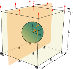
Figure 23: A cube with a sphere inclusion

Table 6: Material properties of a cube with a spherical inclusion

	Young’s modulus $E\left[\mathrm{MPa}\right]$	Poisson’s ratio $\nu$	$\delta_{n}^{\mathrm{o}}/\delta_{s}^{\mathrm{o}}/\delta_{t}^{\mathrm{o}}\left[\mathrm{m}\right]$	$\delta_{m}^{\mathrm{f}}\left[\mathrm{m}\right]$
Cube	$5$	0.25	-	-
Sphere	$1$	0.25	-	-
Cohesive layer	$2$	-	$0.00005$	$0.01$

Two analyses are performed. In one analysis, the model is created with built-in elements of ABAQUS only (referred to as ABAQUS model below). In the other analysis, the model includes SBFEM user elements (referred to as SBFEM model). The ABAQUS model is shown in Fig. 24a. It features a coarser mesh for the sphere, which makes the interface meshes non-conforming. In the SBFEM model, matching meshes are generated by re-meshing the interfacial surfaces, as shown in Fig. 24b. The re-meshing operation yields polyhedral elements, which can be easily handled deploying the SBFEM-based user elements. The interface meshes before and after the re-meshing of an octant (highlighted in Fig. 24a) are depicted in Fig. 25.

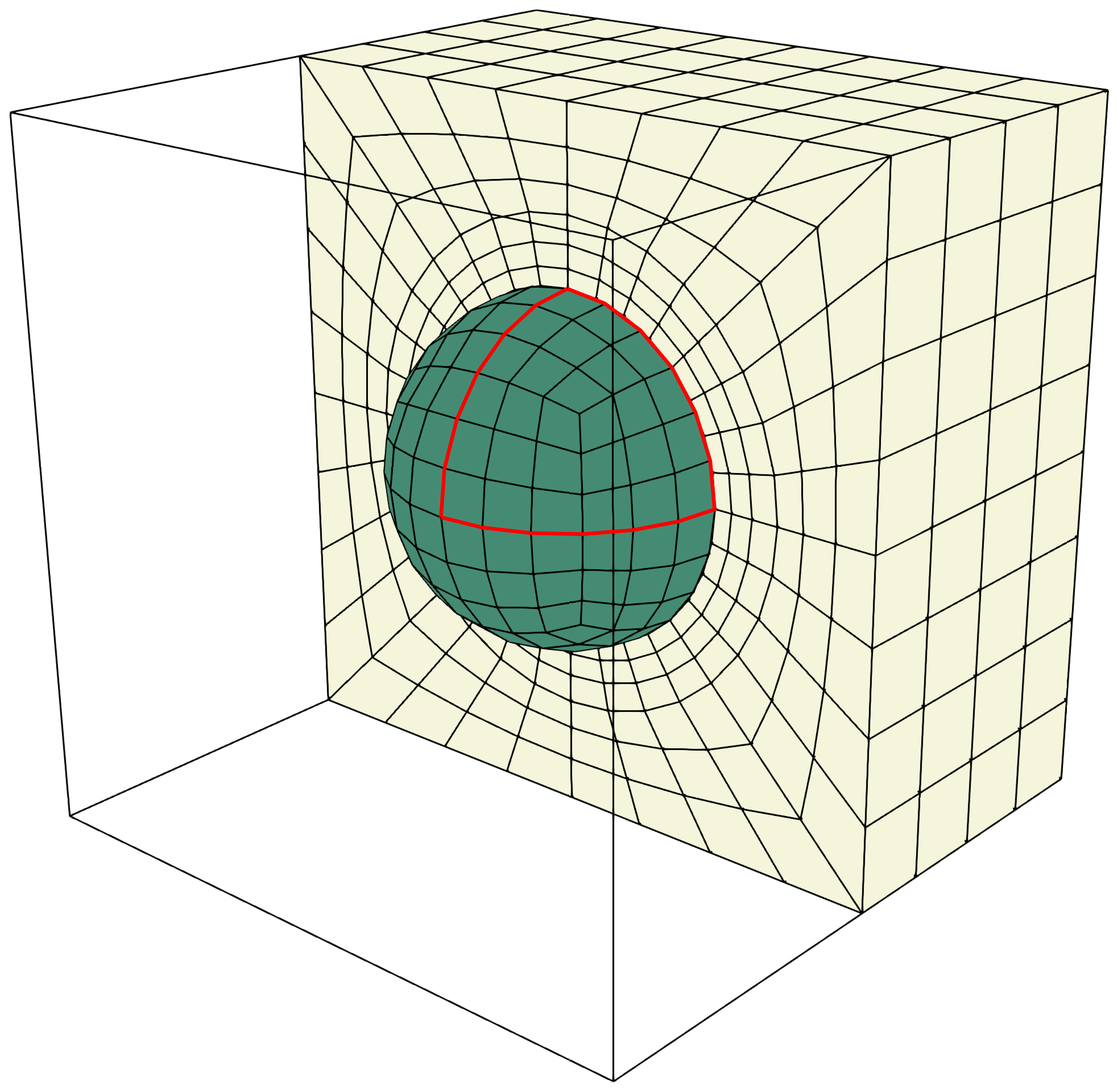
(a) Non-matching meshes

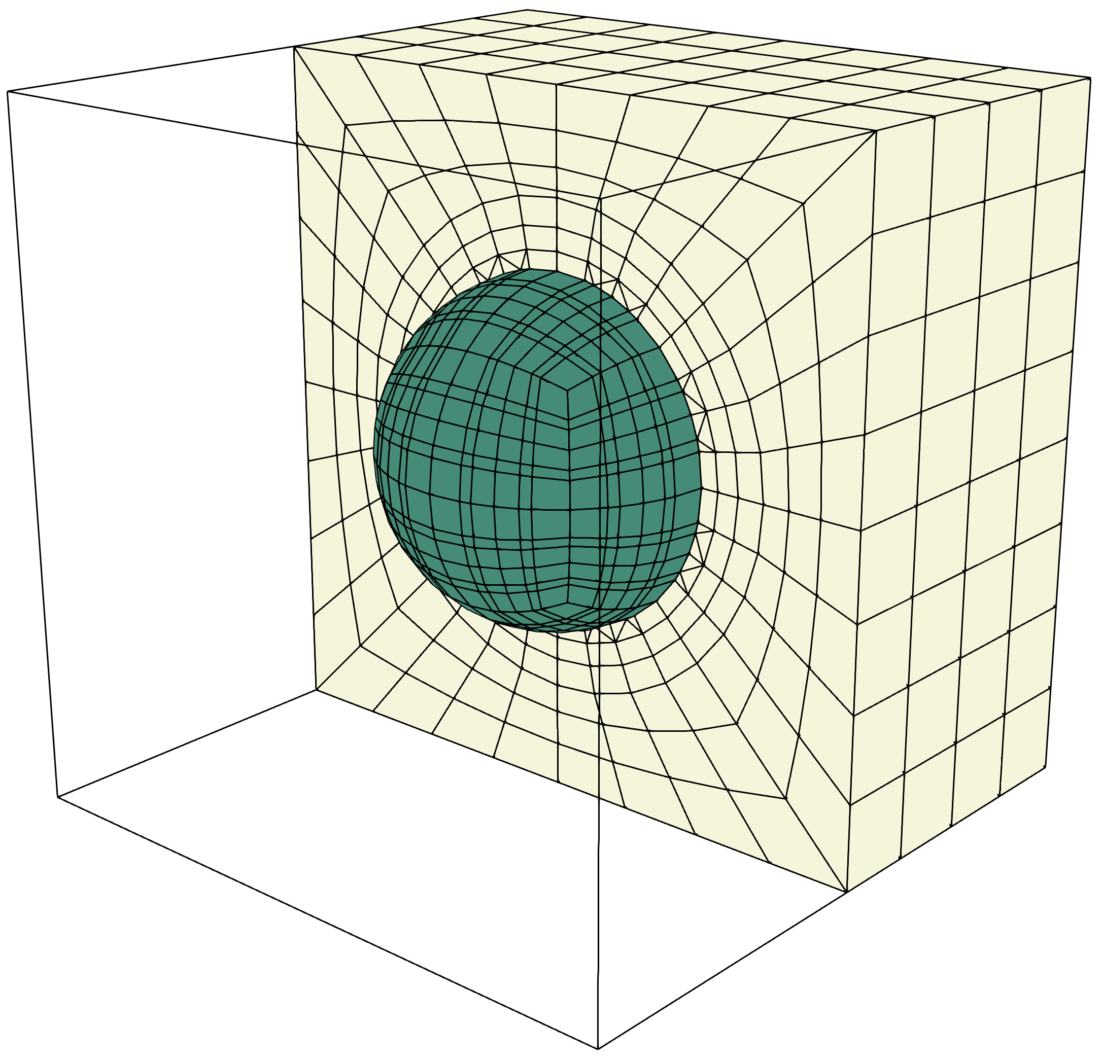
(b) Matching meshes

Figure 24: Meshes of a cube with spherical inclusion

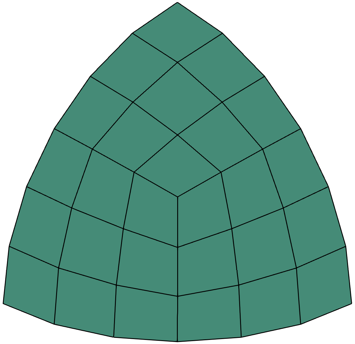
(a) Interface mesh on sphere

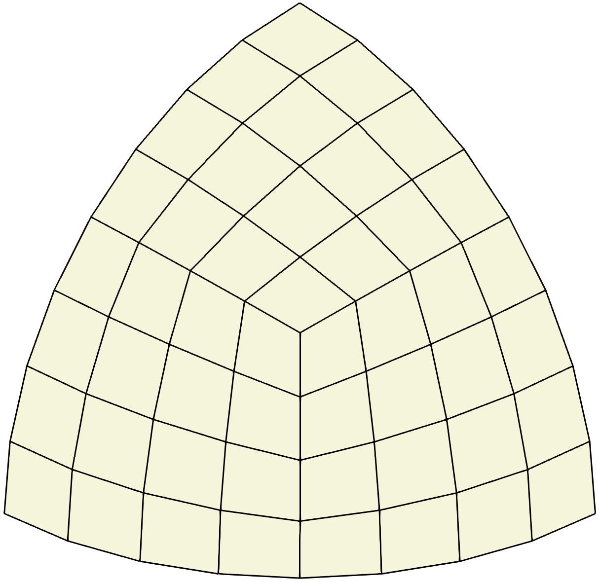
(b) Interface mesh on cube

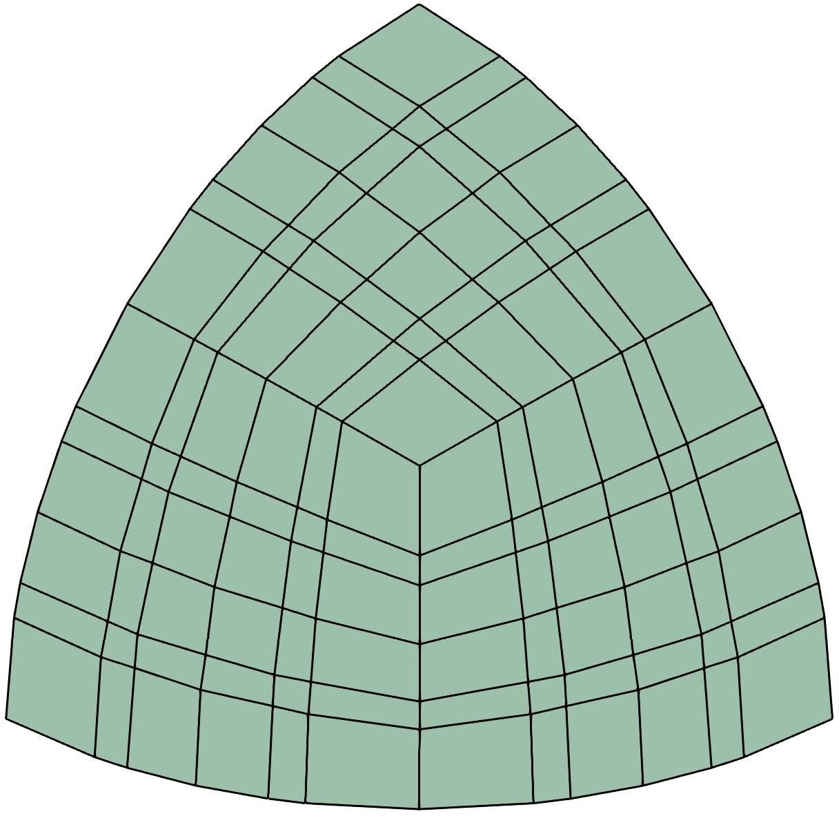
(c) Matching interface mesh

Figure 25: Details of matching meshes of an octant

In the ABAQUS model, there are 3,168 C3D8 elements and 4,471 nodes. The cohesive layer is represented by 384 COH3D8 elements, which are conforming to the inner surface of the cube. The cohesive layer in this model has a thickness of 1$\mathrm{\mu m}$ and it is connected to the two solid blocks by tie constraints. In the SBFEM model, only the surface meshes are adjusted in the re-meshing, thus the number of solid elements does not change. The interfaces are discretized into 864 matching quadrilaterals, which form 864 COH3D8 elements and 1728 overlaid elements. The total number of nodes of the matching mesh is 4,827. As discussed before, the cohesive elements formed by matching meshes have zero thickness and no constraint is required to connect them with adjacent elements. A reference solution is also obtained using ABAQUS built-in elements and a matching mesh. The reference model consists of 201,800 C3D8 elements and 6,144 COH3D8 elements.

The values for the normal traction $t_{n}$ of the cohesive elements obtained from the three models are compared in Fig. 26. Note that the parameter S33 in ABAQUS denotes the normal traction $t_{n}$ of three-dimensional cohesive element. The contour of the SBFEM model is smoother compared to the ABAQUS model, and it is closer to the reference solution.

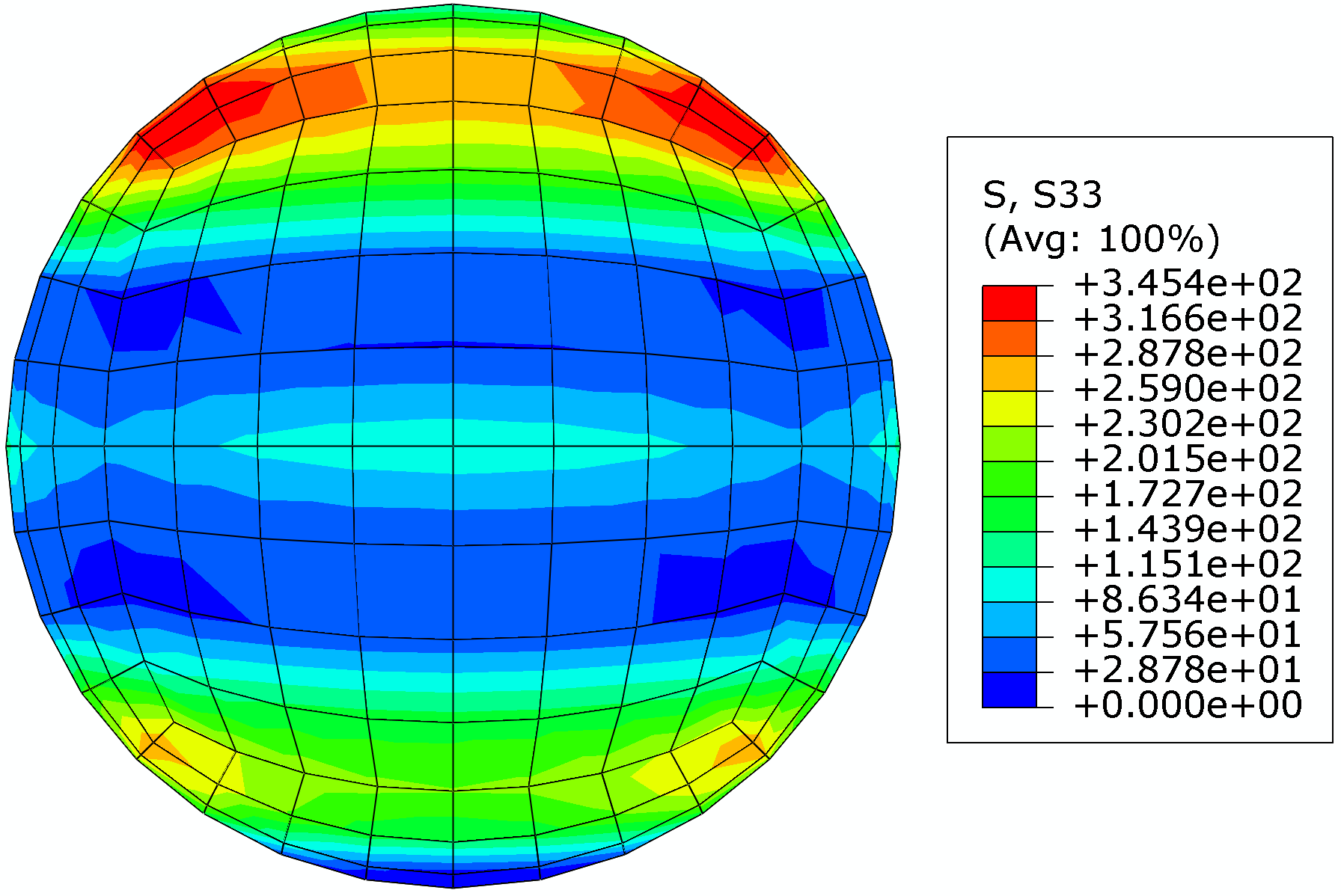
(a) ABAQUS model

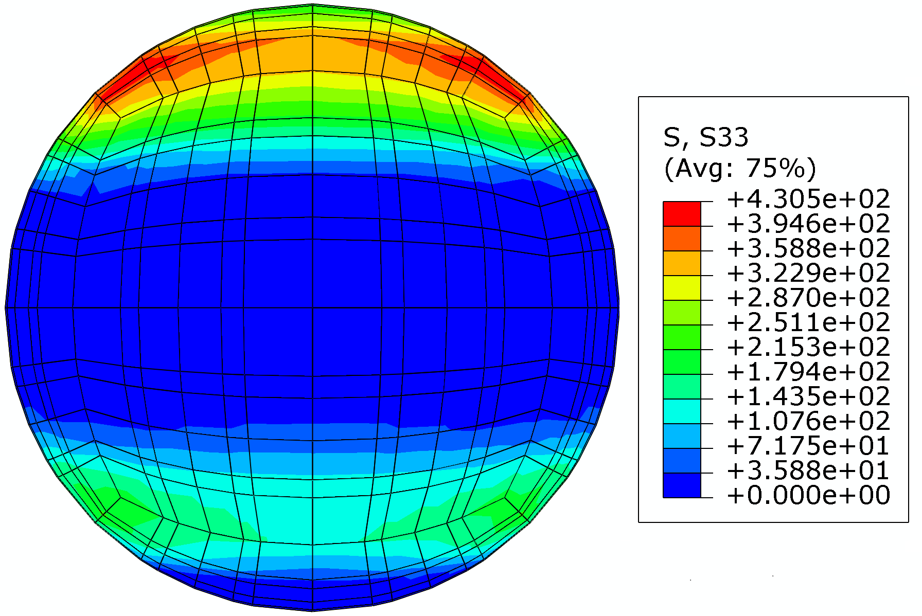
(b) SBFEM model

(c) Reference model

Figure 26: Comparison of the traction contours of cohesive elements (Unit: Pa)

The interaction occurring at the interface along the designated path is plotted in Fig. 27. A positive value indicates the interaction is traction, whereas a negative value denotes the interaction is contact. The horizontal axis is the angle $\theta$ denoted in Fig. 23. As we can see in the figure, the result of the SBFEM model is more accurate than that of the ABAQUS model for both traction and contact zones. At the region $\text{$\pi$}/3<\theta<2\pi/3$, the interaction value is 0, which indicates the cohesive elements around this region have been damaged completely.

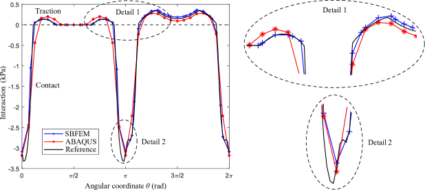
Figure 27: Interaction stress comparison in Y-Z plane

The computational times for the ABAQUS and SBFEM models are compared in Table 7. Because the increment size setting affects the computational time, the default automatic setting of ABAQUS [35] is applied for both models. For the SBFEM model, a pre-calculation step is created before the actual analysis step to obtain stiffness and mass matrices, as discussed in Section 3.1. The time used for the element analysis of UEL comprises of both the time consumed in the pre-calculation and the time in the actual step of analysis. For this problem, the $\mathrm{UEL}$ time accounts for only 18.2% of the total CPU time. The SBFEM model, which has matching interfacial meshes, converges faster than the ABAQUS model. As a result, the SBFEM model requires 15 increments to complete the analysis while the ABAQUS model requires 36 increments. The amount of CPU time saved from the iterative solution is much larger than the extra time spent on the element analysis of UEL. Using the SBFEM model leads to a 70.8% saving of the total CPU time from the ABAQUS model.

Table 7: Comparison of computational times (s) for non-linear analysis

Model	No. of elements	UEL time	ABAQUS solution time	Total CPU time
ABAQUS	3552	-	-	373.70
SBFEM	5824	19.90	89.4	109.30

Apart from the convenience of inserting cohesive elements, the matching meshes have obvious higher accuracy and efficiency compared to the non-matching ones, especially for curved surfaces. The matching meshes are efficient for the numerical simulation of curved ITZs, which commonly exist in composite materials.

4.3 Examples for automatic mesh generation

In previous studies, the octree algorithm has been proven to be a robust and fully automatic mesh generation approach [24, 25]. This technique generates octree cells by recursively subdividing one cell into eight smaller ones of equal size until only one material exists in one cell or a certain threshold is reached. Despite its robustness, the application of octree algorithms has been hindered in conventional FEM due to the issue of hanging nodes.

SBFEM user elements, which allow highly flexible shapes, are complementary to the meshes generated by the octree algorithm. Their combination provides a promising technique for integrating geometric models and numerical analysis in a fully automatic manner. In recent years, octree algorithms have been successfully employed in the SBFEM to generate polyhedral meshes based on digital images [28, 66] and STL models [29]. They are extremely simple and efficient in meshing complex geometries such as concrete and sculptures. Especially the STL-based automatic mesh generation approach is capable of handling curved boundaries by trimming the octree cells [29].

As commercial software, ABAQUS has powerful non-linear solver and it allows parallel equation solution, which benefits the solutions of interfacial problems, especially for geometrically complex problems. Besides, ABAQUS provides comprehensive contact approaches and offers enriched element library that we can combine SBFEM user element with. Especially the contact cohesive behavior and cohesive element, those robust algorithms can be utilized for simulating the traction-separation response occurring in interfacial problems.

In this section, two numerical examples are presented to show the possibilities of using octree cells in ABAQUS in conjunction with our user elements. The first example performs a quasi-static analysis of a porous asphalt concrete specimen meshed by the image-based octree algorithm, in which the interface stripping is simulated by cohesive elements. In the second example, contact analysis is performed on a knee joint meshed by the STL-based octree algorithm with trimming.

4.3.1 Analysis of a porous asphalt concrete specimen

Interface stripping is a common distress appeared in asphalt mixture due to the adhesive failure, which is commonly simulated through cohesive elements in ABAQUS [67]. The internal states of the asphalt mixtures can be obtained from high-resolution X-CT scans and processed by digital image processing techniques [68, 67]. The microstructure can be reconstructed by octree meshes based on the digital images in a fully automatic manner [66, 28]. A porous asphalt concrete specimen is illustrated in Fig. 28a, which is represented by digital images consisting of $200\times 200\times 200$ voxels. The image is a part of the X-CT scans of an asphalt concrete specimen from Ref. [68]. In the figure, the black, gray, and white phases represent the aggregates, asphalt mastic, and air-voids, respectively.

The images can be decomposed automatically using the octree structure, as explained in Ref. [28]. The discretization of the asphalt concrete specimen is shown in Fig. 28b. The elements representing air-voids are removed. At the interface, cohesive elements are inserted for the simulation of the stripping damage, and STS contact with a friction coefficient 0.5 [67] is assigned to prevent interpenetration. The minimum and maximum element sizes are $2^{3}$ and $16^{3}$ voxels, respectively, and the size of one pixel is $0.1\,\mathrm{mm}$. There are 539,170 polyhedral user elements, 208,880 cohesive elements, and 909,402 nodes in the model. The number of nodes in one polyhedral element varies from 8 to 26. The main feature of such octree meshes is the meshes at the interfaces between material phases are fine. Besides, the interfacial meshes are conforming naturally. The meshes having such features can be constructed by the SBFEM user elements, and they are exactly the meshes required for the simulation of the ITZs as discussed in the previous section.

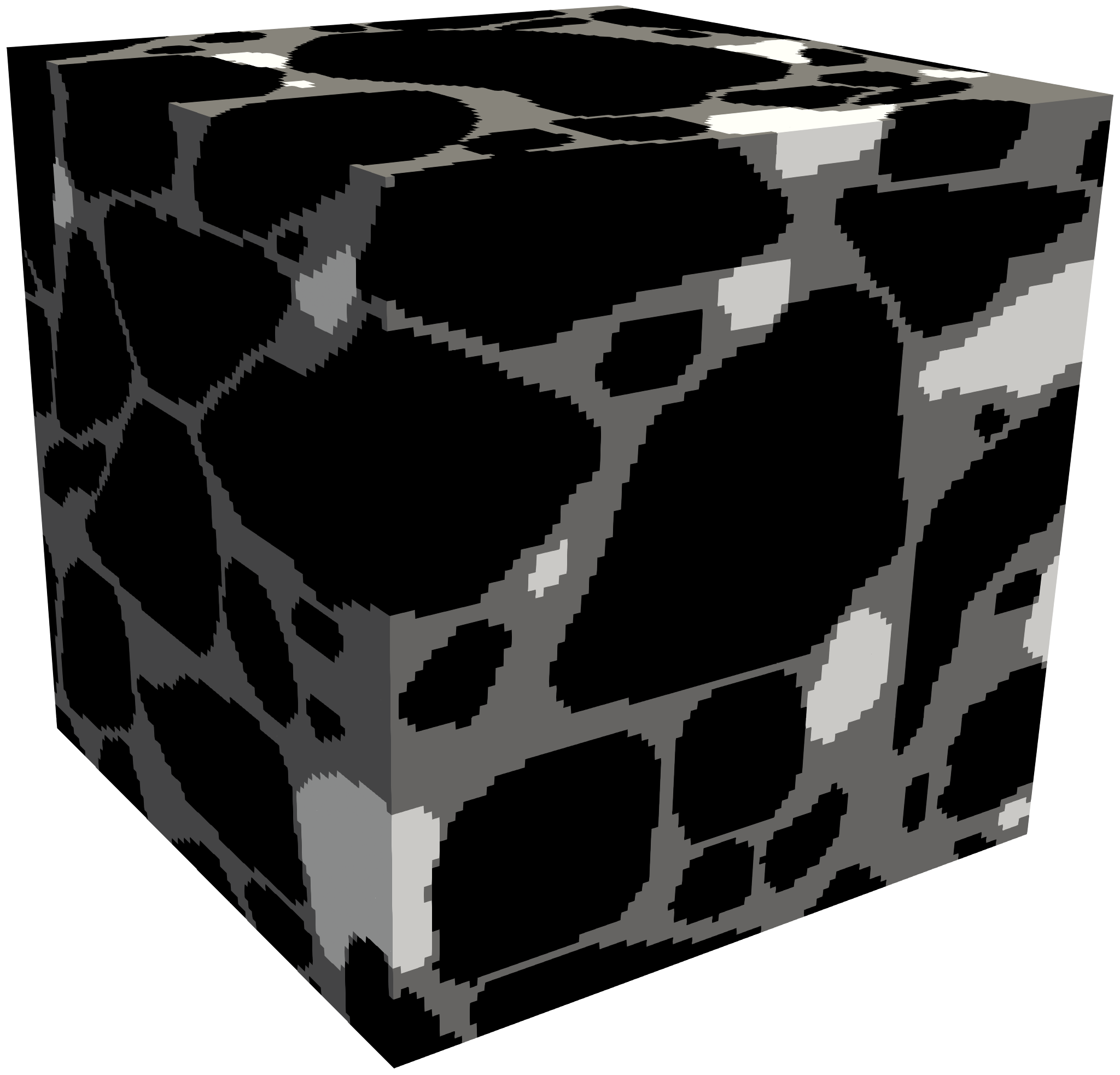
(a) Digital image [68]

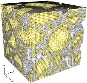
(b) Mesh

Figure 28: A three-dimensional asphalt concrete specimen

The mechanical properties used in this examples are listed in Table 8, in which the viscoelasticity of the asphalt mastic is not taken into consideration. The interface has the same damage behaviors in the normal and two tangential directions, and allows a maximum traction $4\,\mathrm{MPa}$ in each direction. Because the dynamic modulus is often adapted for the asphalt mastic [68], a quasi-static analysis is performed on the model. The bottom of the concrete specimen is fixed, and the vertical planes are constrained for the simulation of confinement. A displacement controlled load up to $-0.5\,\mathrm{mm}$ is applied on the top surface with a loading rate $0.02\,\mathrm{mm}/\mathrm{s}$.

Table 8: Material properties of a porous asphalt concrete specimen

	Young’s modulus $E\left[\mathrm{MPa}\right]$	Poisson’s ratio $\nu$	Density $\rho\left[\mathrm{kg/m^{3}}\right]$	$\delta_{n}^{\mathrm{o}}/\delta_{s}^{\mathrm{o}}/\delta_{t}^{\mathrm{o}}\left[\mathrm{mm}\right]$	$\delta_{m}^{\mathrm{f}}\left[\mathrm{mm}\right]$
Aggregate [67]	$55000$	0.25	2400	-	-
Asphalt mastic [69]	$500$	0.40	2000	-	-
Interface [67]	$20000$	-		$0.0002$	$0.0125$

The stress and damage states of the cohesive elements at the end are depicted in Fig. 29. From Fig. 29a we can see, the Mises stress has reached up to $9.459\,\mathrm{MPa}$ in some area, which may cause damage initiation. The damage contour in Fig. 29b (the parameter SDEG in ABAQUS represents the scalar damage value $D$) shows clearly that the damage has occurs at the interface. In some areas, the damage value reaches to 1, where the interface has complete failure. Those areas are concentrated at the edges of interface or smooth interfaces. This phenomenon is reasonable, because the damage in the normal and tangential directions tends to initiate at the edges of interface and smooth interfaces, respectively.

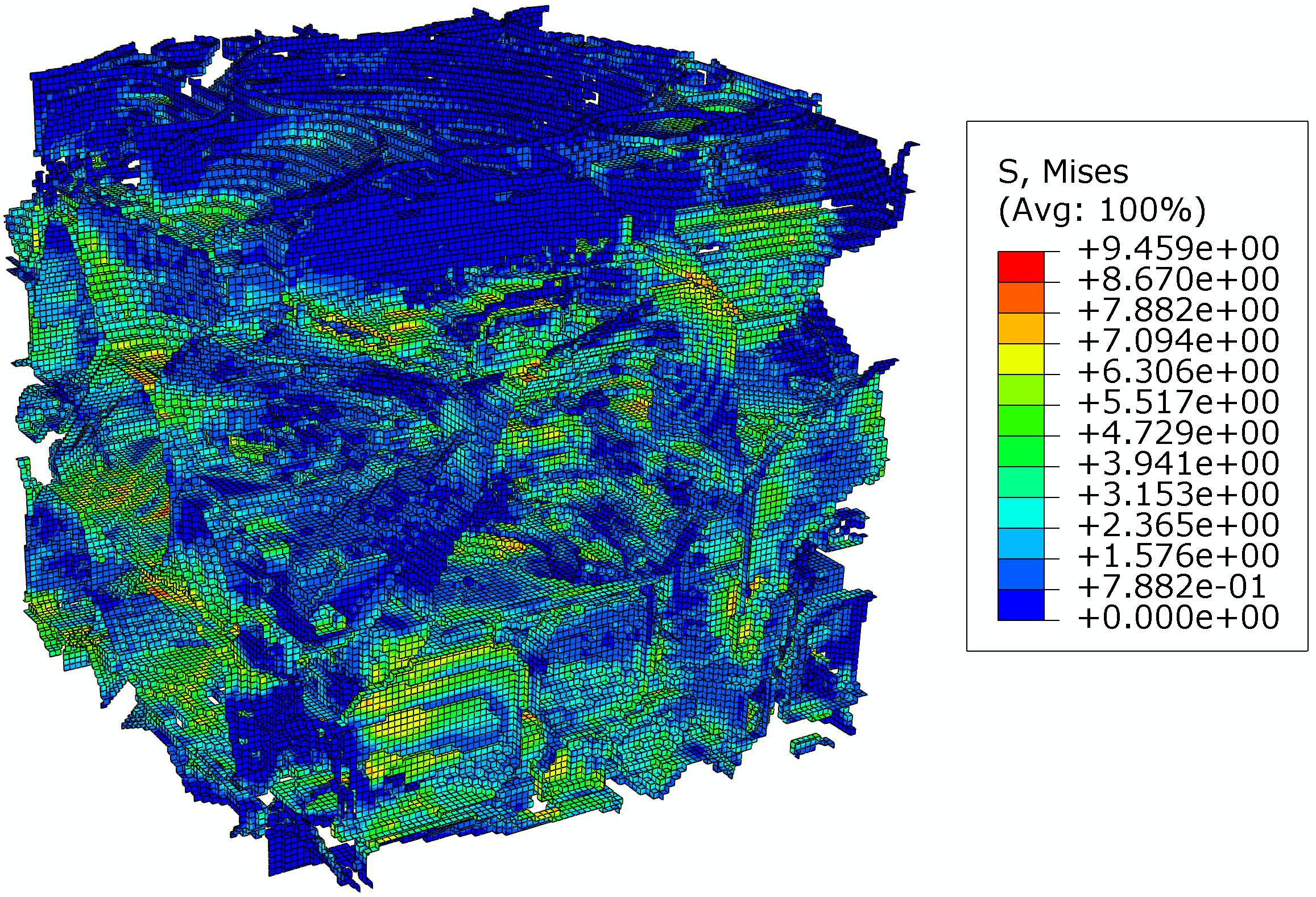
(a) Mises stress contour (Unit: MPa)

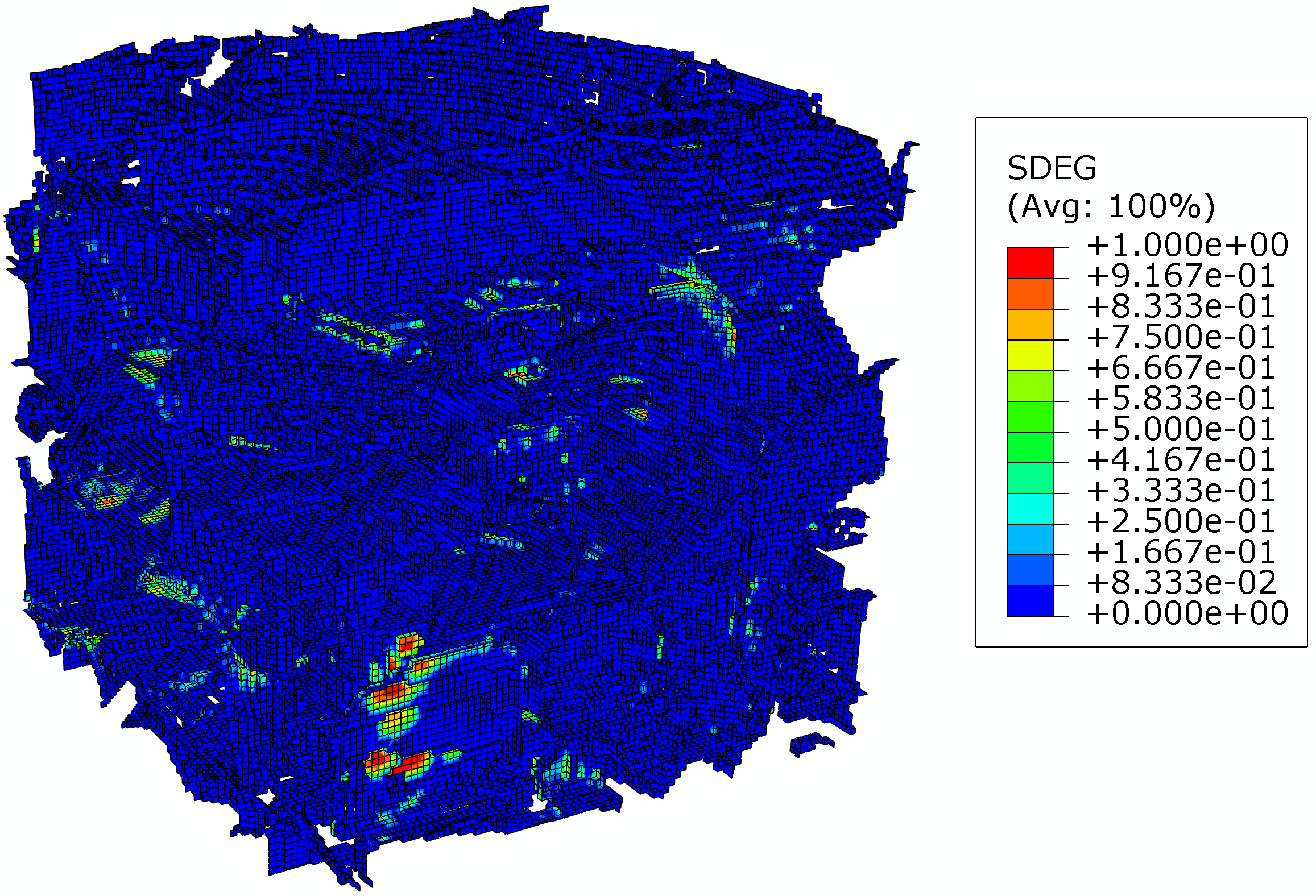
(b) Damage contour

Figure 29: Interface behaviors of a porous asphalt concrete specimen

The total CPU time of this example is 233.51 hours, in which 11.48 hours are spent on the element analysis of UEL. The UEL time comprises of 1.96 hours on the pre-calculation and 9.52 hours on the step of nonlinear analysis. It accounts for only 4.9% of the total CPU time.

4.3.2 Analysis of a knee joint

A knee joint given in STL format [70] is considered for performing a contact analysis. The knee joint is composed of femur and tibia, a meniscus and two articular cartilages as illustrated in Fig. 30. The femur and the tibia are covered with articular cartilages, thus the interactions between bones and articular cartilages can be treated as perfect bond (tie constraint in ABAQUS). The meniscus is inserted into the articular cartilage covering the tibia, thus the interaction between them can also be regarded as perfect bond. The interaction between the meniscus and the articular cartilage covering the femur is treated as contact.

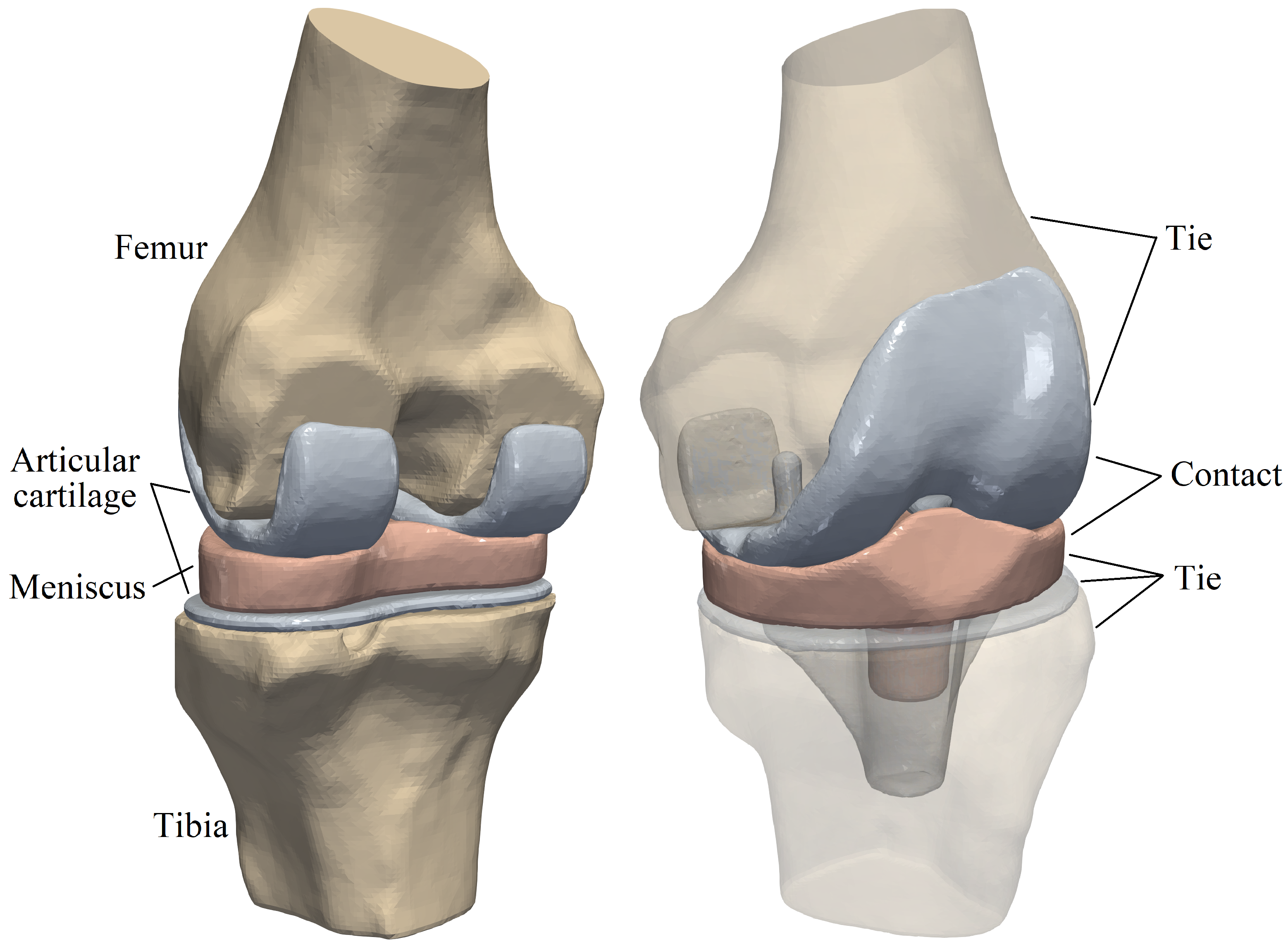
Figure 30: Geometry of a knee model

The mesh generated by the octree algorithm with trimming [29] is shown in Fig. 31. The base sizes are $0.75\,\mathrm{mm}$ and $1\,\mathrm{mm}$ for the contact parts and other parts, respectively. There are 253,079 elements and 361,296 nodes, and the number of nodes in one element varies from 4 to 27. A slice in the vertical plane passing the geometrical center is also shown in Fig. 31. The contact interface meshes are non-matching for this example, because the contact domains are geometrically non-conforming and large sliding might occurs at the interface during the loading process. The meshes generated through the STL-based octree algorithm are suitable for contact analysis. In the standard FEM, local mesh refinement may be required to generate finer meshes on the contact surfaces. However, in an automatic manner, octree cells with fast mesh size transition can be generated through the octree mesh generation technique. Compared to the interior elements, the elements near the boundaries are smaller, which will generate more accurate surfaces for tie constraints and contact pairs. Besides, compared to the image-based technique, the STL-based octree algorithm allows trimming on the octree cells, which leads to more accurate meshes representing complex boundaries especially for curved shapes.

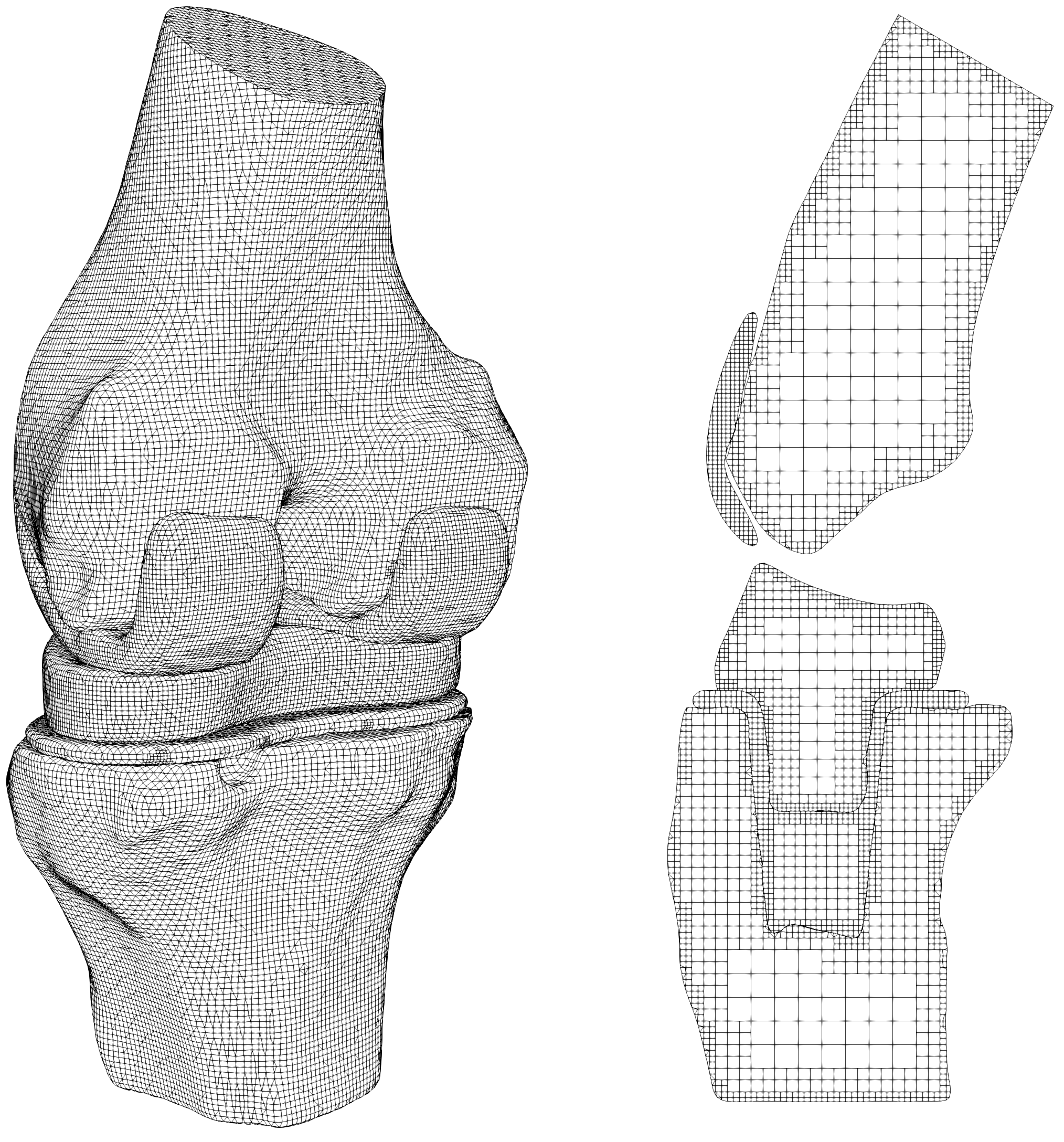
Figure 31: Knee mesh generated by octree algorithm with trimming

The tissue material properties in the computational modeling of human knee joints have been studied in Ref. [71], however, there are considerable variations of the material properties within the wide body of literature. The mechanical properties used in this example are mainly taken from Ref. [72] and are listed in Table 9. The contact is STS contact with a friction coefficient of $\mu=0.05$ [73].

Table 9: Material properties of the knee joint [72]

	Femur	Tibia	Articular cartilage	Meniscus
Young’s modulus $E\left[\mathrm{MPa}\right]$	$20,000$	$20,000$	$30$	$2$
Poisson’s ratio $\nu$	0.2	0.2	0.25	0.35

The bottom surface of the tibia head is fixed, and two translational DOFs in the horizontal plane of the top surface of the femur head are also constrained. On the top surface of the femur head, a vertical load $F$ of up to $1000\,\mathrm{N}$ [72] is applied to induce contact in the knee joint. The displacement contours ($F=1000\,\mathrm{N}$) from different views are shown in Fig. 32. It is obvious that the deformation occurs mainly in the meniscus. The femur, tibia and articular cartilages are similar to rigid bodies. This phenomenon meets the expectation because the Young’s modulus of the meniscus is significantly smaller than those of the bones and articular cartilages. The meniscus is squeezed into the joint space and there is lateral extension of the meniscus. The large deformation of the meniscus increases the contact area which is helpful to reduce the contact pressure.

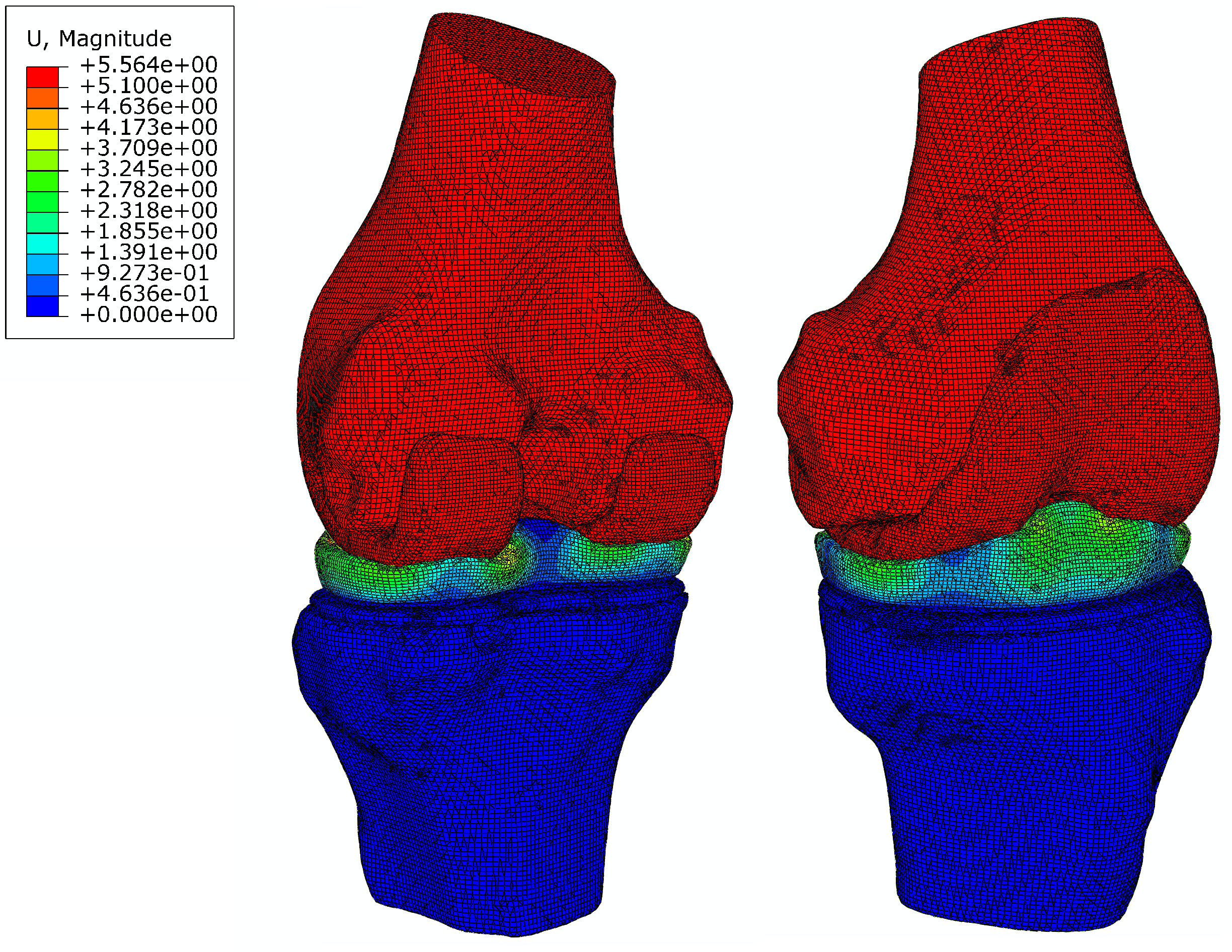
Figure 32: Displacement contours of the knee joint (Unit: $\mathrm{mm}$)

The contact pressure distributions ($F=1000\,\mathrm{N}$) are depicted in Fig. 33. To illustrate the distribution clearly, contact pressure values smaller than $10^{-4}\,\mathrm{MPa}$ are not included in the contour. It is obvious that the contact pressure on the articular cartilage has a similar distribution and magnitude compared to that on the meniscus. Besides, the contact pressure on the articular cartilage has a similar distribution from Ref. [72].

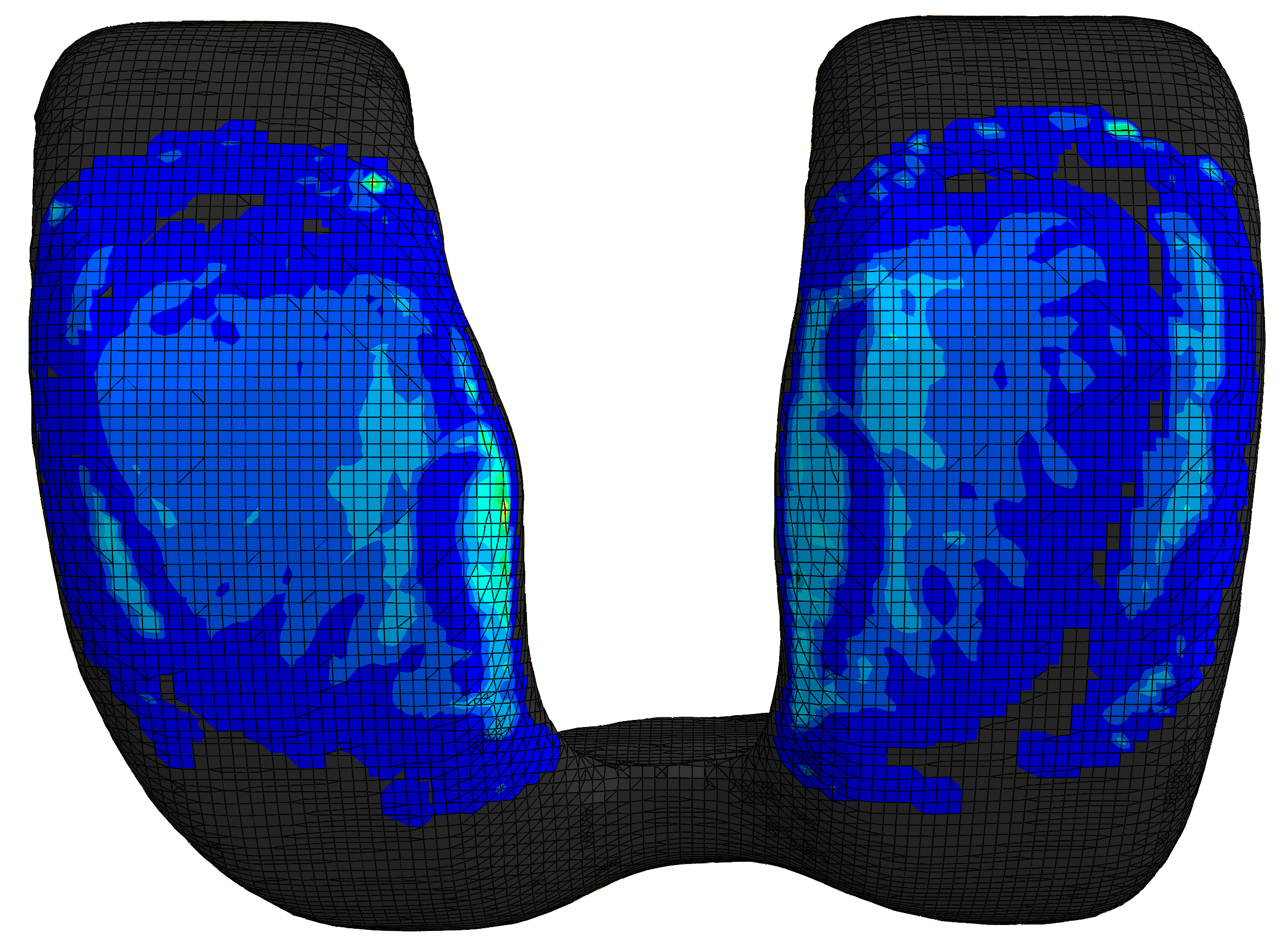
(a) Contact pressure on articular cartilage

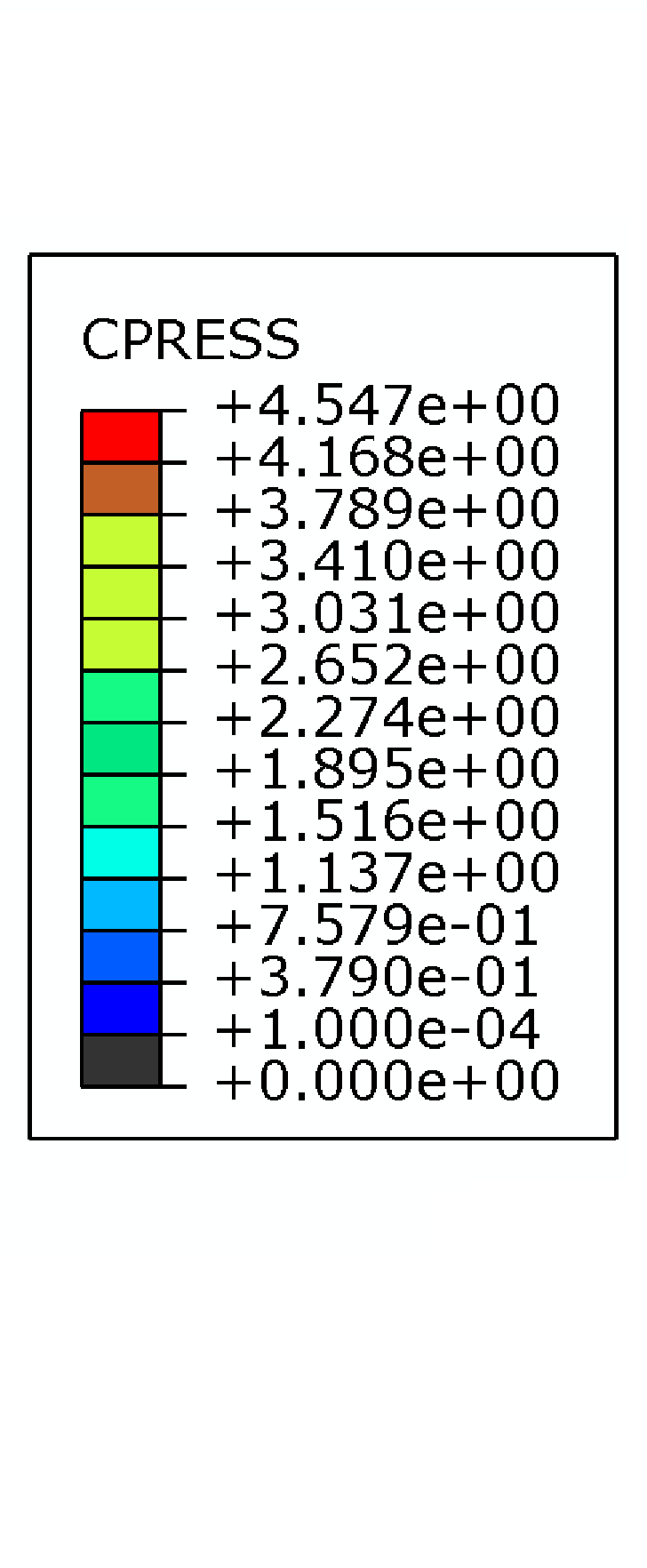
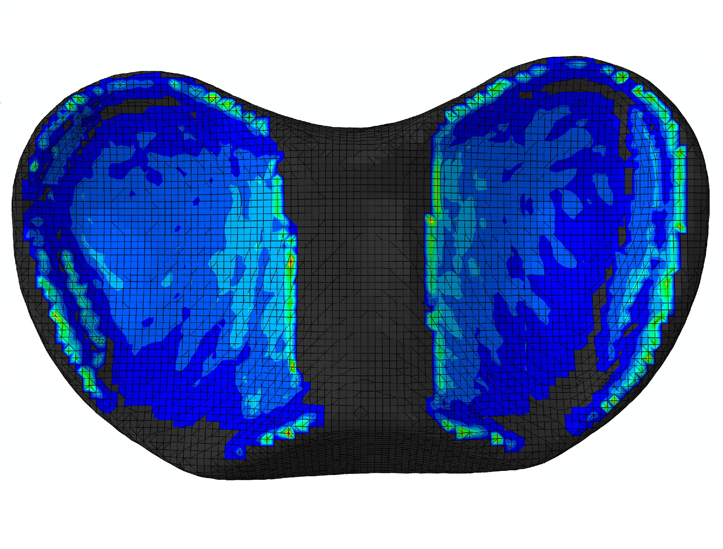
(b) Contact pressure on meniscus

Figure 33: Contact pressure of knee joint (Unit: $\mathrm{MPa}$)

The development of the contact on the articular cartilage is recorded, as depicted in Fig. 34. Note that only the area where the contact pressure is greater than $10^{-4}\,\mathrm{MPa}$ has been taken into account. Generally speaking, with increasing the vertical load $F$, the contact area is increasing while its increasing rate is reducing. The average contact pressure increases during the loading history. Before the vertical load increases up to $650\,\mathrm{N}$, the increasing rate of the average contact pressure is basically reducing. However, when $F>650\,\mathrm{N}$ the average contact pressure increases almost linearly because the contact area increases only slightly.

(a) Contact Area

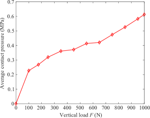
(b) Average contact pressure

Figure 34: Development of the contact on the articular cartilage

The total CPU time of this example is 16.68 hours, in which 0.90 hours are spent on the element analysis of UEL. The UEL time comprises of 0.52 hours on the pre-calculation and 0.38 hours on the step of nonlinear analysis. It accounts for only 5.4% of the total CPU time.

5 Conclusion

In this paper, a polyhedral element based on the SBFEM is implemented as a user element within the commercial finite element software ABAQUS. The implementation involves the user subroutines $\mathrm{UEXTERNALDB}$ and $\mathrm{UEL}$ to store the topology and perform the calculations of the polyhedral element, respectively. The required data structures for storing the polyhedral mesh and the elemental topology have been presented and described in detail. A comprehensive explanation of the framework of the $\mathrm{UEL}$ has been provided in conjunction with the theoretical derivations needed for the implementation. Furthermore, a modified approach of overlaying standard elements on the SBFEM user elements is proposed to create element-based surfaces, which allows establishing interactions for interfacial problems.

The availability of polyhedral user elements enhances the performances of ABAQUS for interfacial problems, and it significantly reduces the meshing burden encountered in the standard FEM. To verify the implementation, three benchmark tests (static, modal, and transient) are performed. It is observed that very accurate results are obtained when compared to theoretical and numerical reference solutions. The advantages of polyhedral elements, i.e., the flexibility of dealing with non-matching meshes and its compatibility with automatic mesh generation techniques, are illustrated by five numerical examples. By introducing matching meshes for complex geometries consisting of several parts featuring different element sizes, the performance of existing contact modeling approaches in ABAQUS can be significantly enhanced. Matching meshes provide interface representations without initial gaps or penetrations, and thus, zero thickness cohesive elements for the simulation of ITZs in the composite materials can be easily inserted. The SBFEM user elements are highly complementary to octree-based mesh generation techniques, which are efficient and robust to mesh complex geometries and promising for integrating geometric models and numerical analysis in a fully automatic manner.

In a nutshell, the SBFEM user element will enable ABAQUS users to benefit from the advantages of this method. The commercial FEM software ABAQUS offers a user-friendly interface and outstanding nonlinear solvers, which will facilitate the use of the SBFEM to scholars. The source code of the implementation is chosen to be published open-source governed by the GPLv3 license, it can be downloaded from https://github.com/ShukaiYa/SBFEM-UEL with several input files of numerical examples presented in the paper.

References

- [1] A. Fawkes, D. Owen, and A. Luxmoore. An assessment of crack tip singularity models for use with isoparametric elements. Engineering Fracture Mechanics, 11(1):143–159, 1979.
- [2] F. Medina and R. L. Taylor. Finite element techniques for problems of unbounded domains. International journal for numerical methods in engineering, 19(8):1209–1226, 1983.
- [3] P. K. Banerjee and R. Butterfield. Boundary element methods in engineering science, volume 17. McGraw-Hill London, 1981.
- [4] C. Song and J. P. Wolf. The scaled boundary finite-element method-alias consistent infinitesimal finite-element cell method-for elastodynamics. Computer Methods in Applied Mechanics and Engineering, 147(3):329–355, 1997.
- [5] T. Belytschko and T. Black. Elastic crack growth in finite elements with minimal remeshing. International journal for numerical methods in engineering, 45(5):601–620, 1999.
- [6] J. P. Wolf and C. Song. Finite-element modelling of unbounded media. Wiley Chichester, 1996.
- [7] M. H. Bazyar and C. Song. A continued-fraction-based high-order transmitting boundary for wave propagation in unbounded domains of arbitrary geometry. International Journal for Numerical Methods in Engineering, 74(2):209–237, 2008.
- [8] A. A. Saputra, C. Birk, and C. Song. Computation of three-dimensional fracture parameters at interface cracks and notches by the scaled boundary finite element method. Engineering Fracture Mechanics, 148:213–242, 2015.
- [9] C. Song, E. T. Ooi, and S. Natarajan. A review of the scaled boundary finite element method for two-dimensional linear elastic fracture mechanics. Engineering Fracture Mechanics, 187:45–73, 2018.
- [10] K. O. Coelho, P. R. B. Devloo, and S. M. Gomes. Error estimates for the scaled boundary finite element method. arXiv preprint arXiv:2012.13418, 2020.
- [11] L. Lehmann, S. Langer, and D. Clasen. Scaled boundary finite element method for acoustics. Journal of Computational Acoustics, 14(4):489–506, 2006.
- [12] C. Birk, L. Liu, and C. Song. Coupled acoustic response of two-dimensional bounded and unbounded domains using doubly-asymptotic open boundaries. Journal of Computational Physics, 310:252–284, 2016.
- [13] W. Xing, C. Song, and F. Tin-Loi. A scaled boundary finite element based node-to-node scheme for 2D frictional contact problems. Computer Methods in Applied Mechanics and Engineering, 333:114–146, 2018.
- [14] W. Xing, J. Zhang, C. Song, and F. Tin-Loi. A node-to-node scheme for three-dimensional contact problems using the scaled boundary finite element method. Computer Methods in Applied Mechanics and Engineering, 347:928–956, 2019.
- [15] J. Liu, J. Li, P. Li, G. Lin, T. Xu, and L. Chen. New application of the isogeometric boundary representations methodology with SBFEM to seepage problems in complex domains. Computers and Fluids, 174:241–255, 2018.
- [16] E. T. Ooi, C. Song, and F. Tin-Loi. A scaled boundary polygon formulation for elasto-plastic analyses. Computer Methods in Applied Mechanics and Engineering, 268:905–937, 2014.
- [17] Z. Zhang, D. Dissanayake, A. Saputra, D. Wu, and C. Song. Three-dimensional damage analysis by the scaled boundary finite element method. Computers & Structures, 206:1–17, 2018.
- [18] Hirshikesh, A. L. N. Pramod, R. K. Annabattula, E. T. Ooi, C. Song, and S. Natarajan. Adaptive phase-field modeling of brittle fracture using the scaled boundary finite element method. Computer Methods in Applied Mechanics and Engineering, 355:284–307, 2019.
- [19] J. Zhang, S. Natarajan, E. T. Ooi, and C. Song. Adaptive analysis using scaled boundary finite element method in 3d. Computer Methods in Applied Mechanics and Engineering, Accepted for publication on 08/08/2020, 2020.
- [20] S. Natarajan, J. Wang, C. Song, and C. Birk. Isogeometric analysis enhanced by the scaled boundary finite element method. Computer Methods in Applied Mechanics and Engineering, 283:733–762, 2015.
- [21] J. Eisenträger, J. Zhang, C. Song, and S. Eisenträger. An SBFEM approach for rate-dependent inelasticity with application to image-based analysis. International Journal of Mechanical Sciences, page 105778, 2020.
- [22] J. Liu, P. Zhang, G. Lin, W. Wang, and S. Lu. Solutions for the magneto-electro-elastic plate using the scaled boundary finite element method. Engineering Analysis with Boundary Elements, 68:103–114, 2016.
- [23] W. Ye, J. Liu, G. Lin, B. Xu, and L. Yu. Application of scaled boundary finite element analysis for sloshing characteristics in an annular cylindrical container with porous structures. Engineering Analysis with Boundary Elements, 97:94–113, 2018.
- [24] M. A. Yerry and M. S. Shephard. Automatic three-dimensional mesh generation by the modified-octree technique. International Journal for Numerical Methods in Engineering, 20(11):1965–1990, 1984.
- [25] M. S. Shephard and M. K. Georges. Automatic three-dimensional mesh generation by the finite octree technique. International Journal for Numerical Methods in Engineering, 32(4):709–749, 1991.
- [26] D. M. Greaves and A. G. L. Borthwick. Hierarchical tree-based finite element mesh generation. International Journal for Numerical Methods in Engineering, 45(4):447–471, 1999.
- [27] E. T. Ooi, H. Man, S. Natarajan, and C. Song. Adaptation of quadtree meshes in the scaled boundary finite element method for crack propagation modelling. Engineering Fracture Mechanics, 144:101–117, 2015.
- [28] A. Saputra, H. Talebi, D. Tran, C. Birk, and C. Song. Automatic image-based stress analysis by the scaled boundary finite element method. International Journal for Numerical Methods in Engineering, 109(5):697–738, 2017.
- [29] Y. Liu, A. A. Saputra, J. Wang, F. Tin-Loi, and C. Song. Automatic polyhedral mesh generation and scaled boundary finite element analysis of STL models. Computer Methods in Applied Mechanics and Engineering, 313:106–132, 2017.
- [30] Y. Huang, Z. Yang, W. Ren, G. Liu, and C. Zhang. 3D meso-scale fracture modelling and validation of concrete based on in-situ X-ray computed tomography images using damage plasticity model. International Journal of Solids and Structures, 67-68:340–352, 2015.
- [31] J. Zhang and C. Song. A polytree based coupling method for non-matching meshes in 3D. Computer Methods in Applied Mechanics and Engineering, 349:743–773, 2019.
- [32] L. Liu, J. Zhang, C. Song, C. Birk, A. A. Saputra, and W. Gao. Automatic three-dimensional acoustic-structure interaction analysis using the scaled boundary finite element method. Journal of Computational Physics, 395:432–460, 2019.
- [33] ANSYS Inc. ANSYS Mechanical APDL Programmer’s Reference. Southpointe, 275 Technology Drive, Canonsburg, PA, U.S.A, 2013.
- [34] MSC MARC. Volume D: User Subroutines and Special Routines. Santa Ana, CA, U.S.A, 2005.
- [35] ABAQUS. ABAQUS 2016 Documentation. Dassault Systémes Simulia Corp., Providence, RI, U.S.A, 2015.
- [36] J. Shi, J. Lua, H. Waisman, P. Liu, T. Belytschko, N. Sukumar, and Y. Liang. X-FEM toolkit for automated crack onset and growth prediction. In 49th AIAA/ASME/ASCE/AHS/ASC Structures, Structural Dynamics, and Materials Conference, page 1763, 2008.
- [37] M. McNary. Implementation of the extended finite element method (XFEM) in the ABAQUS software package. PhD thesis, Georgia Institute of Technology, 2009.
- [38] E. Giner, N. Sukumar, J.E. Tarancón, and F. J. Fuenmayor. An ABAQUS implementation of the extended finite element method. Engineering Fracture Mechanics, 76(3):347–368, 2009.
- [39] T. Elguedj, A. Duval, F. Maurin, and H. Al-Akhras. ABAQUS user element implementation of NURBS based isogeometric analysis. In 6th European congress on computational methods in applied sciences and engineering, Vienna, Austria, pages 10–14, 2012.
- [40] X. Cui, X. Han, S. Duan, and G. Liu. An ABAQUS implementation of the cell-based smoothed finite element method (CS-FEM). International Journal of Computational Methods, 17(02):1850127, 2020.
- [41] P. Y. Kumbhar, A. Francis, N. Swaminathan, R. K. Annabattula, and S. Natarajan. Development of user element routine (UEL) for cell-based smoothed finite element method (CSFEM) in ABAQUS. International Journal of Computational Methods, 17(02):1850128, 2020.
- [42] Z. Yang, F. Yao, and Y. Huang. Development of ABAQUS UEL/VUEL subroutines for scaled boundary finite element method for general static and dynamic stress analyses. Engineering Analysis with Boundary Elements, 114:58–73, 2020.
- [43] C. Song. The Scaled Boundary Finite Element Method: Introduction to Theory and Implementation. John Wiley & Sons, 2018.
- [44] E. T. Ooi, C. Song, and S. Natarajan. Construction of high-order complete scaled boundary shape functions over arbitrary polygons with bubble functions. International Journal for Numerical Methods in Engineering, 108(9):1086–1120, 2016.
- [45] E. T. Ooi, A. Saputra, S. Natarajan, E. H. Ooi, and C. Song. A dual scaled boundary finite element formulation over arbitrary faceted star convex polyhedra. Computational Mechanics, 66(1):27–47, 2020.
- [46] S. Duczek, A. A. Saputra, and H. Gravenkamp. High order transition elements: The xNy-element concept—Part I: Statics. Computer Methods in Applied Mechanics and Engineering, 362:112833, 2020.
- [47] O. C. Zienkiewicz and R. L. Taylor. The finite element method, Volume 1: Basic formulation and linear problems. 4 edition, 1994.
- [48] L. Chen, B. Simeon, and S. Klinkel. A NURBS based Galerkin approach for the analysis of solids in boundary representation. Computer Methods in Applied Mechanics and Engineering, 305:777–805, 2016.
- [49] C. Arioli, A. Shamanskiy, S. Klinkel, and B. Simeon. Scaled boundary parametrizations in isogeometric analysis. Computer Methods in Applied Mechanics and Engineering, 349:576–594, 2019.
- [50] C. Song. A matrix function solution for the scaled boundary finite-element equation in statics. Computer Methods in Applied Mechanics and Engineering, 193(23):2325–2356, 2004.
- [51] C. Van Loan. A symplectic method for approximating all the eigenvalues of a Hamiltonian matrix. Linear Algebra and its Applications, 61:233–251, 1984.
- [52] CD-adapco S. STAR-CCM+ User Guide version 12.04. CD-adapco, 60 Broadhollow Road, Melville, NY, U.S.A, 2017.
- [53] ANSYS Inc. ANSYS Fluent User’s Guide. Southpointe, 275 Technology Drive, Canonsburg, PA, U.S.A, 2013.
- [54] A. Abdelkader, C. L. Bajaj, M. S. Ebeida, A. H. Mahmoud, S. A. Mitchell, J. D. Owens, and A. A. Rushdi. VoroCrust: Voronoi meshing without clipping. arXiv preprint arXiv:1902.08767, 2019.
- [55] A. H. Squillacote, J. Ahrens, C. Law, B. Geveci, K. Moreland, and B. King. The ParaView guide, volume 366. Kitware Clifton Park, NY, U.S.A, 2007.
- [56] E. Anderson, Z. Bai, C. Bischof, L. S. Blackford, J. Demmel, J. Dongarra, J. Du C., A. Greenbaum, S. Hammarling, A. McKenney, and Danny S. LAPACK Users’ Guide. Society for Industrial and Applied Mathematics, Philadelphia, PA, U.S.A, 3 edition, 1999.
- [57] O. Astrachan. Bubble sort: An archaeological algorithmic analysis. ACM Sigcse Bulletin, 35(1):1–5, 2003.
- [58] H. M. Hilber, T. J. R. Hughes, and R. L. Taylor. Improved numerical dissipation for time integration algorithms in structural dynamics. Earthquake Engineering & Structural Dynamics, 5(3):283–292, 1977.
- [59] N. Garg, N. D. Chakladar, B. G. Prusty, C. Song, and A. W. Phillips. Modelling of laminated composite plates with weakly bonded interfaces using scaled boundary finite element method. International Journal of Mechanical Sciences, 170:105349, 2020.
- [60] C. M. López, I. Carol, and A. Aguado. Meso-structural study of concrete fracture using interface elements. I: numerical model and tensile behavior. Materials and structures, 41(3):583–599, 2008.
- [61] S. Huzni, M. Ilfan, T. Sulaiman, S. Fonna, M. Ridha, and A. K. Arifin. Finite element modeling of delamination process on composite laminate using cohesive elements. International Journal of Automotive and Mechanical Engineering, 7:1023, 2013.
- [62] C. Sarrado, F. A. Leone, and A. Turon. Finite-thickness cohesive elements for modeling thick adhesives. Engineering Fracture Mechanics, 168:105–113, 2016.
- [63] W. Trawiński, J Tejchman, and J Bobiński. A three-dimensional meso-scale modelling of concrete fracture, based on cohesive elements and x-ray ct images. Engineering fracture mechanics, 189:27–50, 2018.
- [64] D. W. Spring and G. H. Paulino. A growing library of three-dimensional cohesive elements for use in ABAQUS. Engineering Fracture Mechanics, 126:190–216, 2014.
- [65] J. Segurado and J. Llorca. A numerical approximation to the elastic properties of sphere-reinforced composites. Journal of the Mechanics and Physics of Solids, 50(10):2107–2121, 2002.
- [66] A. A. Saputra, S. Eisenträger, H. Gravenkamp, and C. Song. Three-dimensional image-based numerical homogenisation using octree meshes. Computers & Structures, 237:106263, 2020.
- [67] J. Hu, P. Liu, D. Wang, M. Oeser, and G. Canon Falla. Investigation on interface stripping damage at high-temperature using microstructural analysis. International Journal of Pavement Engineering, 20(5):544–556, 2019.
- [68] J. Hu, Z. Qian, D. Wang, and M. Oeser. Influence of aggregate particles on mastic and air-voids in asphalt concrete. Construction and Building Materials, 93:1–9, 2015.
- [69] W. G. Buttlar, D. Bozkurt, G. G. Al-Khateeb, and A. S. Waldhoff. Understanding asphalt mastic behavior through micromechanics. Transportation Research Record, 1681(1):157–169, 1999.
- [70] ISIFC Biomedical school. Knee prosthesis model. https://www.thingiverse.com/thing:340254, 2014.
- [71] A. E. Peters, R. Akhtar, E. J. Comerford, and K. T. Bates. Tissue material properties and computational modelling of the human tibiofemoral joint: a critical review. PeerJ, 6:e4298, 2018.
- [72] Y. Wang, Y. Fan, and M. Zhang. Comparison of stress on knee cartilage during kneeling and standing using finite element models. Medical engineering & physics, 36(4):439–447, 2014.
- [73] L. McCann, E. Ingham, Z. Jin, and J. Fisher. Influence of the meniscus on friction and degradation of cartilage in the natural knee joint. Osteoarthritis and Cartilage, 17(8):995–1000, 2009.