Computing foaming flows across scales:
from breaking waves to microfluidics

Abstract

Crashing ocean waves, cappuccino froths and microfluidic bubble crystals are examples of foamy flows. Foamy flows are critical in numerous natural and industrial processes and remain notoriously difficult to compute as they involve coupled, multiscale physical processes. Computations need to resolve the interactions of the bubbles with the fluid and complex boundaries, while capturing the drainage and rupture of the microscopic liquid films at their interface. We present a novel multilayer simulation framework (Multi-VOF) that advances the state of the art in simulation capabilities of foamy flows. The framework introduces a novel scheme for the distinct handling of multiple neighboring bubbles and a new regularization method that produces sharp interfaces and removes spurious fragments. Multi-VOF is verified and validated with experimental results and complemented with open source, efficient scalable software. We demonstrate capturing of bubble crystalline structures in realistic microfluidics devices and foamy flows involving tens of thousands of bubbles in a waterfall. The present multilayer framework extends the classical volume-of-fluid methodology and allows for unprecedented large scale, predictive simulations of flows with multiple interfaces.

Main

Bubbly foams are the signature of violent crashes of ocean waves and happy times accompanied by champagne. Bubble coalescence and collapse is central to new products and technologies in areas ranging from food, to cosmetics and drug delivery through precision microfluidics for emulsions and foams [34, 1, 28]. Drainage and rupture of the liquid film separating bubbles leads to their coalescence. Surfactants [16] and other impurities, such as electrolytes [13], in the liquid can delay or prevent coalescence. Bubbles in clean liquids can also collide without coalescence if the film drainage time is sufficiently large [9]. Foams are composed by many bubbles separated by stable liquid films. Foams are structural elements of insect, fish and frog nests and central to numerous industrial processes and medicine [35, 21, 17].

The simulation of foamy flows, involving non-coalescing bubbles, presents a number of formidable challenges in addition to those associated with resolving the bubble interactions with the fluid flow and the solid boundaries [36]. In foams the thickness of the film is usually several orders of magnitude smaller than the size of bubbles. In the limit of zero film thickness, the evolution of (dry) foams can be predicted using Lagrangian techniques that track the surfaces between bubbles with multiple junctions [7]. State of the art techniques involve Eulerian methods such as the Voronoi Implicit Interface Method (VIIM) [32] that uses a single level-set function for all interfaces. More recently, methods such as the Lattice Boltzmann  [27] have captured the effect of thin films using an empirical collision potential but resort to mesoscale models with limited density ratio and artificial compressibility. In simulations of bubble collisions in turbulent flows [18], a short range repulsive force between bubbles has been used to increase the surface tension near the contact. However, this can only remedy rapid collisions but not account for stable multi-bubble structures with thin films as in foams.

The classical volume-of-fluid (VOF) methodology [22, 29] has found widespread success in simulations of engineering flows involving interfaces. However, VOF leads to spurious coalescence of bubbles that approach each other at a distance below one computational cell. Such spurious coalescence can be prevented by introducing distinct volume fraction fields for each bubble in the multi-marker volume-of-fluid [4] or distinct functions in level-set methods [12]. This prevention of coalescence has a computational cost that is proportional to the number of bubbles in the simulation (i.e. $\mathcal{O}(N_{\mathrm{bubbles}}\,N_{\mathrm{cells}})$), and it is prohibitive for systems with a few hundred bubbles even in today’s computer architectures. Furthermore as each distinct volume fraction field corresponds to only one bubble keeping track of all volume fraction fields is redundant. We propose a method to store multiple fields in a compact way so that the number of the necessary scalar fields is constant, independent on the number of bubbles in the simulation (see Methods). This technique is combined with VOF to simulate flows with non-coalescing bubbles. The proposed multilayer volume-of-fluid method (Multi-VOF) overcomes the above mentioned challenges and allows for predictive simulations of flows involving thousands of interacting and non-coalescing bubbles. Multi-VOF requires only a fixed number of fields, and its computational cost is independent on the number of bubbles in the simulation.

Results

Constrained mean curvature flow, comparison with VIIM

The capabilities of Multi-VOF are first assessed in the limiting case of fluid flows with surface tension but no inertia. In this case the governing equations (see  Methods) simplify to a single equation for the velocity field $\bm{u}=\kappa\nabla\alpha-\nabla p$, where the scalar field $p(\bm{x},t)$ is used to ensure that the velocity field is divergence-free ($\nabla\cdot\bm{u}=0$). We use this velocity field with the advection equation to compare Multi-VOF with the pioneering work in [32]. The initial conditions are adopted from [32] and represent a Voronoi diagram of a randomly chosen set of 100 points with homogeneous Neumann boundary conditions for the volume fraction fields. Initially, the interfaces are straight lines and form multiple junctions at arbitrary angles. As time evolves, only triple junctions remain and the angles between the lines approach $120^{\circ}$. In Fig. 1, we compare the solution by our method and the Voronoi Implicit Interface Method [32]. For Multi-VOF, dry foams are a limiting case since there is no special treatment of triple junctions leading to the formation of small voids near the junctions. Nevertheless, the results are of Multi-VOF and VIIM are in excellent agreement for the same mesh size. Applying penalization techniques can further improve the results by removing the voids.

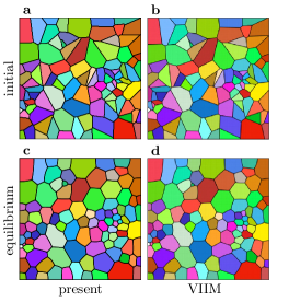
Figure 1: Constrained mean curvature flow. The initial field (a,b) is a Voronoi diagram. Multi-VOF method (c) produces results similar to that of the Voronoi implicit interface method (VIIM) [32] (d) on the same mesh of $256^{2}$ cells. Interfaces at triple junctions form $120^{\circ}$ angles.

Microfluidic crystals

Bubbles and droplets in microfluidic devices organize into lattices called microfluidic crystals [5]. They serve as prototypes of foam structures, compartments for chemical reactions, and parts in production of metamaterials [25]. A recent study [27] applied a mesoscale lattice Boltzmann (LB) model to capture these flow structures. The LB model includes a short range forcing term that describes the combined effect of surface tension and near-contact interactions to prevent coalescence. The authors compare their results with experimental data [25] on foams of air bubbles in water. However, due to the limited density ratio of the LB approach, their mesoscale model is instead tuned for water drops embedded in oil.

Using the Multi-VOF method, we aim to reproduce the experimental study [31] on the formation of microfluidic crystals of bubbles in water. Limited by numerical stability and computational cost, we use lower values of the density ratio, surface tension, viscosity and the channel length. The device is based on a flow-focusing geometry [20] and consists in a planar network of rectangular ducts of height $H$ with three inlets. The gas is injected from one inlet at a fixed pressure $P_{g}$ relative to the outlet pressure, and the liquid comes through the other two with a total flow rate $Q_{l}$. The gas enters the channel through a contracting duct that ends with an orifice of a width $W_{0}$ expanding into the collection channel. Walls of the channel are no-slip boundaries. Parameters of the simulation are given in Supplementary Table LABEL:supp_t_crystal.

Bubbles in such devices are generated by the breakup of the air thread in the inlet channel. The period of breakup is determined by the liquid flow rate and not by capillary time scales despite an apparent similarity to the Rayleigh-Plateau instability [20]. In simulations, we forcibly separate the air thread at a regular interval $T_{b}$. Unless stated otherwise, the period of breakup equals $T_{b}=0.5\,W_{0}^{2}H/Q_{l}$ estimating the time it takes for the liquid to fill the volume of a cavity forming right before the breakup.

To obtain various crystalline structures, we vary the inlet gas pressure $P_{g}$. The gas flow rate $Q_{g}$ and the bubble volume $V_{b}$ as functions of pressure are plotted in Fig. 2. The gas flow starts as soon as the pressure exceeds the capillary threshold estimated as $P_{\mathrm{cap}}=\sigma\big{(}\frac{1}{H}+\frac{1}{W_{0}}\big{)}$. Raising the pressure enhances the gas flow rate $Q_{g}$ and, since the breakup period $T_{b}$ is kept constant, increases the size of bubbles. Each simulation with a given $P_{g}$ is advanced until equilibration, the evolution of the gas flow rate for selected values of $P_{g}$ is shown in Supplementary Figure LABEL:supp_f_crystal_volume. Closely packed bubbles form $120^{\circ}$ angles at triple junctions, and junctions at the walls are $90^{\circ}$. Depending on the size, the bubbles organize into regular structures, or flowing crystals. The structures are named by the number of bubbles that fit in the channel width [31]: hex-one, hex-two, hex-three and so on. Examples of the structures together with experimental images are shown in Fig. 2 and Movies S1-S4. Stability of each structure is dictated by the corresponding value of the surface energy. Smaller bubbles transition to higher-order structures.

The dissipation in foam is proportional to its wetting perimeter, i.e. the length of the menisci that confine the liquid between the interface and the channel walls [8]. Hex-one bubbles dissipate more than hex-two bubbles and correspond to a slower flow [31]. Our simulations capture this effect as seen from Fig. 2 and Movie S5. If the structure remains the same, increasing the pressure leads to a faster flow. Conversely, if the structure changes, increasing the pressure may decrease the flow rate. For example, increasing $P_{g}$ from $205\;\mathrm{Pa}$ to $216\;\mathrm{Pa}$ reduces the flow rate as the flow transitions from hex-two to hex-one.

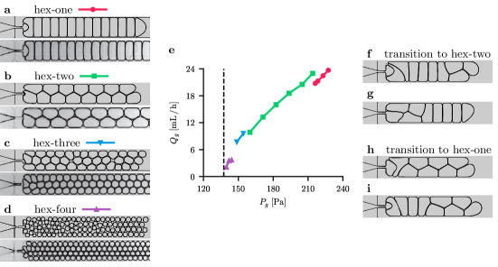
Figure 2: (a-d) Crystalline structures of bubbles from simulations compared to experimental images [31]. Hex-one ($P_{g}=216\;\mathrm{Pa}$, a), hex-two ($P_{g}=194\;\mathrm{Pa}$, b), hex-three ($P_{g}=149\;\mathrm{Pa}$, c), and hex-four ($P_{g}=140\;\mathrm{Pa}$, d). (e) Gas flow rate as a function of the inlet gas pressure. The flow starts once the pressure exceeds the capillary threshold   . Lines correspond to hex-one   , hex-two   , hex-three   , and hex-four    structures. (f-g) Spontaneous transitions between hex-one and hex-two with $L=5.3\;\mathrm{mm}$ and $P_{g}=225\;\mathrm{Pa}$. Snapshots are taken at times $443\;\mathrm{ms}$ (f), $460\;\mathrm{ms}$ (g), $512\;\mathrm{ms}$ (h), and $529\;\mathrm{ms}$ (i).

One behavior observed near such transitions is a bubbling oscillator [30]. It is based on the interplay between the stability and dissipation of hex-one and hex-two structures. As the channel fills with hex-one bubbles, the flow rate decreases due to growing dissipation. The bubbles entering the channel become smaller such that the hex-one structure is no longer stable. The flow transitions to hex-two and accelerates again. The process repeats indefinitely. In our simulations, we obtain such an oscillator with $L=5.3\;\mathrm{mm}$, $T_{b}=0.46\,{W_{0}^{2}H}/{Q_{l}}$ and the inlet pressure $P_{g}=225\;\mathrm{Pa}$. The flow rate plotted in Supplementary Figure LABEL:supp_f_crystal_volume oscillates in time. Examples of the transitions between hex-one and hex-two are shown in Fig. 2.

Bidisperse foam generation

A recently demonstrated microfluidic device [37] makes use of bubble-bubble pinch-off to generate bidisperse foams. Here we reproduce its operation numerically. The device represents a planar network $60\;\mu\mathrm{m}$ high where a narrow channel expands with $45^{\circ}$ walls to a collection channel. Bubbles are generated periodically at an interval of $111\;\mu\mathrm{s}$ to maintain the volume fraction of gas at $0.645$. At each cycle, the bubble is inserted in the narrow channel by replacing the liquid with gas in a part of the channel. Parameters of the simulation a summarized in Supplementary Table LABEL:supp_t_microfoam. Walls of the channel are no-slip boundaries.

The overall view of the device is shown in Fig. 3a and Movie S6. The snapshot from the simulation in Fig. 3b compared to the experimental image [37] (Fig. 3d therein) indicates a good agreement with the experimental data since both have similar shapes and positions of the split and intact bubbles.

Bubbles entering the expansion alternate between two types of behavior illustrated in Fig. 3d-i. They either split into smaller bubbles or remain intact. For example, one bubble (Fig. 3d) enters the expansion, elongates under the shear stress (Fig. 3e) from the liquid flow and splits into two daughter bubbles (Fig. 3f). The wall bubble confines the liquid flow. The two daughter bubbles then migrate sideways, leaving a gap of liquid between the wall bubble (Fig. 3g) and the next incoming bubble, which only elongates without breakup and eventually restores its shape. Alternation of these two regimes drives the generation of bidisperse foams.

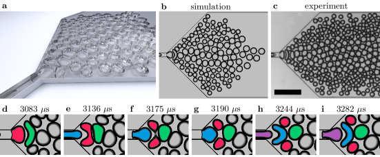
Figure 3: (a) Overall view of the microfluidic device for generation of bidisperse foams at $t=8749~{}\mu\mathrm{s}$. (b) Snapshot from the simulation at $t=8872~{}\mu\mathrm{s}$. (c) Experimental image [37]. The scale bar is $500\;\mu\mathrm{m}$. (d-i) Alternation between bubble-bubble pinch-off and elongation without breakup. snapshots at $t=3083,3136,3175,3190,3244$, and $3282~{}\mu\mathrm{s}$ respectively. Colors highlight the same bubbles in all snapshots. Split bubble (red), wall bubble (green), and intact bubble (blue).

Another part of the pinch-off process is the pincher bubble upstream of the split bubble (blue in Fig. 3e and purple in Fig. 3h). One question arising here is whether the pincher bubble actually causes the breakup. The explanation given in the experimental study [37] suggests that the pincher bubble increases the flow confinement and the corresponding shear stresses on the split bubble, leading to breakup. To verify this, we compare two simulations: one with a normal pinch-off event and one where the pincher bubble is delayed by $60\;\mu\mathrm{s}$. Both simulations were done with the length of the collection channel set to $L=0\;\mu\mathrm{m}$ to reduce the computational cost, still leaving a sufficient separation from the outlet. Fig. 4 shows that the pincher bubble does not trigger the pinch-off event. Delaying the pincher bubble does not change the flow of the liquid near the split bubble (Fig. 4h and Fig. 4k). This indicates that the pinch-off is triggered by the wall bubble downstream rather than the pincher bubble upstream.

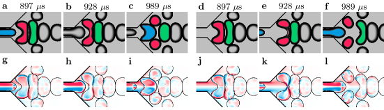
Figure 4: Effect of delaying the pincher bubble. Standard case (a-c, g-i) and case with delayed pincher bubble (d-f, j-l) at various time instances. (a-f) Bubble surfaces with the highlighted pincher bubble (blue), split bubble (red) and wall bubble (green). (g-l) Component of vorticity normal to the view plane (red for counterclockwise and blue for clockwise). Delaying the pincher bubble does not prevent breakup.

Clustering of bubbles

Clustering of bubbles floating on the surface of water is an example of self-assembly known as the Cheerios effect [38], named after the observation that breakfast cereals floating in milk often clamp together. A bubble floating on the surface creates an elevation attracting other bubbles due to buoyancy. Many floating bubbles are hence attracted to each other and form clusters.

Fig. 5 shows clusters of bubbles obtained numerically and experimentally. In the experimental setup, a large tank is filled halfway with tap water and a common detergent. One end of a tube with an inner diameter of about $0.3\;\mathrm{mm}$ is submerged into water, and the other end is connected to a syringe filled with air. The plunger is then abruptly pushed until bubbles start to appear. This generates bubbles of about $2\;\mathrm{mm}$ in diameter. To visualize the deformation of the surface, the bottom of the tank is covered with a patterned sheet. In the simulation, spherical bubbles are generated at the bottom at regular intervals. Parameters are in Supplementary Table LABEL:supp_t_column. Both in the experiment and the simulation, bubbles floating on the surface form clusters and organize in a hexagonal lattice. Movie S7 shows the simulation results.

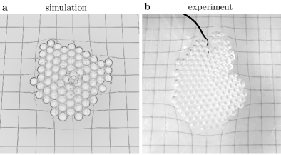
Figure 5: Clustering of bubbles floating on water. (a) Simulation using the Multi-VOF method (b) Experiment in soapy water. The size of square cells is $4\;\mathrm{mm}$.

Foaming waterfall

Natural surfactants in sea water can suppress coalescence as well. Oceans are covered with foam generated by breaking waves. The following application is an example of such flows in the limiting case without coalescence. A rectangular tank $100\;\mathrm{mm}$ high is filled halfway with water. A waterfall enters the tank at a given velocity. Supplementary Table LABEL:supp_t_waterfall lists the simulation parameters. Results of the simulation are in Fig. 6 with additional snapshots in Supplementary Figure LABEL:supp_f_waterfall_series and Movie S8. On the finest mesh consisting of $768\times 384\times 384$ cells, the simulation took 20 hours on 1152 compute nodes of the Piz Daint supercomputer equipped with 12-core CPU Intel Xeon E5-2690 v3 processors. Two major mechanisms of air entrainment [24] are observed in this simulation: entrapment of a tube of air when the sheet of water impacts the surface and entrainment around the impact site as the waterfall drags air into the water. The entrained bubbles rise to the surface and create a layer of foam. As seen from the horizontal cross-section of the foam in Fig. 6, the bubbles are separated by thin membranes (lamellae) that form multiple junctions (Plateau borders) at angles approaching $120^{\circ}$.

The distribution of the bubble size in Fig. 6 matches a scaling law [19] $N(r)\propto r^{-10/3}$, where $N(r)$ is the number of bubbles of radii in the range $r\pm 0.1\;\mathrm{mm}$. The model stems from the assumption that the inflow of air per unit volume is constant, and the number of bubbles depends only on the turbulent dissipation rate and the bubble radius. This scaling law is commonly observed for bubbles generated by breaking waves and has been reported in experimental [14] and numerical [15] studies.

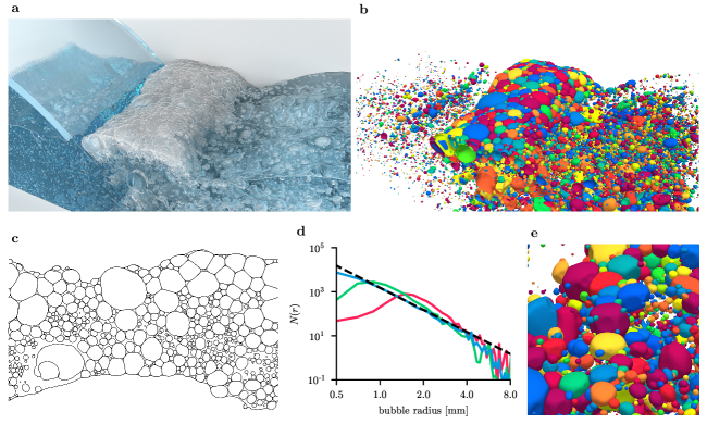
Figure 6: Foaming waterfall. (a) Overall view of the interface at $t=1.2\;\mathrm{s}$. (b) Same view showing bubbles under the surface with arbitrary colors. (c) Horizontal cross-section of the interface at $t=1.2\;\mathrm{s}$. Clusters of bubbles on the surface show characteristic features of foam: bubbles are separated by thin membranes (lamellae) with multiple junctions (Plateau borders). (d) Histogram of the bubble radius. $N(r)$ is the number of bubbles with the equivalent radius in the range $r\pm 0.1\;\text{mm}$. Results for different mesh sizes of $96$   , $192$   , and $384$    cells in the height compared to scaling law [19] $N(r)\propto r^{-10/3}$   . The values are averaged in time over $1<t<1.2\;\mathrm{s}$. (e) Close-up of (b) with half of the bubbles removed.

Discussion

The multilayer volume-of-fluid method can simulate flows with many bubbles and drops that do not coalesce. It represents many bubbles with a fixed number of volume fraction fields and assigns colors to bubbles to distinguish them. An additional technique of interface regularization based on forward-backward advection improves the accuracy of the advection scheme. The presented applications show that the method can reproduce experiments on generation of foam in microfluidic devices and clustering of bubbles floating in water.

The proposed methodology advances the state of the art in simulations of flows with multiple interfaces in the following categories:

1. Efficiency: The method uses a fixed number of volume fraction fields on an Eulerian mesh. The computational complexity of the advection algorithm is linear with the number of cells and does not depend on the number of bubbles.

2. Compatibility with existing methods: The method is compatible with existing stencil-based methods for interface capturing and curvature estimation, including the popular volume-of-fluid and level-set methods.For dry foams, the method can recover the results of VIIM at comparable resolutions.

3. Capturing topology changes and multiple bubble junctions: Breakup and coalescence of bubbles including thin liquid films and triple lines are captured without employing ad-hoc parameters.

4. Coupling with models of film drainage and rupture: Coalescence can be controlled by assigning appropriate color functions to interacting bubbles.

5. High performance implementation: The method only involves stencil operations and is readily integrated in high performance software for structured grids.

We believe that Multi-VOF opens new horizons for simulating a wide variety of flows from the micro to the macroscale, including wet foams, turbulent flows with bubbles, suspensions and emulsions in microfluidics. Moreover, the efficiency of the code allows for extensive studies in control and optimization of bubbly flows.

Limitations

The method describes the complete prevention of coalescence and a an empirical criterion is used in cases where the residence time of bubbles is finite. Since bubbles are distinguished as connected components of the volume fraction field, the method does not prevent coalescence if a deformed bubble folds back onto itself. Two small bubbles can penetrate each other and form concentric configurations when their radius is comparable to one computational cell. The method can be improved by adopting a semi-implicit discretization of the surface tension force [11].

Generation of bubbles requires additional modeling. In simulations, we forcibly separate the air thread at regular intervals. Otherwise, the gas thread remains continuous unless the inlet pressure is sufficiently low. Such continuous regimes are observed experimentally under certain conditions [2] but not in the experimental study of interest [31]. One explanation for this discrepancy is the effect of wetting [2] that may narrow the gap between the liquid-gas interface and the channel walls since the static contact angle of polydimethylsiloxane (PDMS) is $104^{\circ}$ [26] while our model assumes $180^{\circ}$. Another possibility is that the viscous flow of the liquid upstream of the orifice is not sufficiently resolved in the simulations.

Methods

Multilayer fields

Consider a discrete domain $\Omega$ consisting of cells $c\in\Omega$, where the number of cells is $|\Omega|=N_{\mathrm{cells}}$. A conventional cell field $\phi\colon c\mapsto\phi_{c}$ is a mapping from cell $c$ to a value. A cell-color field $\hat{\phi}\colon(c,q)\mapsto\hat{\phi}_{c}(q)$ is a mapping from cell $c$ and color $q\in\mathbb{R}$ to a value. Overlapping bubbles can be represented by a single cell-color field if each bubble is assigned a unique color. The restriction operation $\big{.}\hat{\phi}\big{|}_{q}$ constructs a conventional field $\big{.}\hat{\phi}\big{|}_{q}\colon c\mapsto\hat{\phi}_{c}(q)$ from a cell-color field $\hat{\phi}$ given a color $q$. Using this operation, any standard routine, such as computing the normals or solving the advection equation, can be applied to a cell-color field by individually selecting all possible colors. To store a cell-color field $\hat{\phi}$, we use a sequence of conventional fields for values and colors separately. Assume that any cell contains at most $L$ bubbles and their shapes are represented by the cell-color volume fraction field $\hat{\alpha}$. The colors are stored in fields $q^{l}:c\mapsto q_{c}^{l},\;l=1,\dots,L$ defined in each cell $c$ as

$$q_{c}^{l}=\begin{cases}q_{l},&1\leq l\leq L^{\prime}\,,\\ q_{\mathrm{none}},&\text{otherwise}\,,\end{cases}$$

where $\{q_{1},\dots,q_{L^{\prime}\leq L}\}$ are all colors for which $\hat{\alpha}_{c}(q)>0$ and $q_{\mathrm{none}}$ is a distinguished none color (e.g. $q_{\mathrm{none}}\coloneqq-1$). The corresponding values are stored in fields $\phi^{l}:c\mapsto\phi_{c}^{l},\;l=1,\dots,L$

$$\phi^{l}=\begin{cases}\hat{\phi}(q_{c}^{l}),&q_{c}^{l}\neq q_{\mathrm{none}}\,,\\ \textit{undefined},&\text{otherwise}\,.\end{cases}$$

The pairs $(\phi^{l},q^{l})$ are referred to as layers and the sequences $(\phi^{1},\dots,\phi^{L})$ and $(q^{1},\dots,q^{L})$ constitute a multilayer field. The order in which the colors are stored is insignificant, i.e. all sequences $(q_{c}^{1},\dots,q_{c}^{L})$ and $(\phi_{c}^{1},\dots,\phi_{c}^{L})$ are equivalent up to mutual permutation. Fig. 7 illustrates two layers that describe three overlapping bubbles.

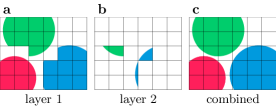
Figure 7: Two-layer volume fraction field representing three bubbles. Individual layers (a,b) contain at most one bubble per cell, while the combined field (c) describes overlapping interfaces.

Advection

By constructing conventional fields from a cell-color field, we can apply standard stencil-based algorithms to cell-color fields. One such algorithm, the PLIC (Piecewise Linear Interface Characterization) method [40] for advection, is described in the following. The PLIC method solves the advection equation given a velocity field $\bm{u}$ $\frac{\partial\alpha}{\partial t}+(\bm{u}\cdot\nabla)\,\alpha=0.$ As the name stands, it performs a piecewise linear reconstruction by replacing the interface in each cell with a plane. Apart from the volume fraction field, it involves normals and plane constants. The normals $\bm{n}:\Omega\rightarrow\mathbb{R}^{3}$ are estimated from the volume fractions using the mixed Youngs-centered scheme [3] and the plane constants are computed from the normals and volume fractions using explicit formulas [33]. The fluid volume is reconstructed in each cell with a polyhedron formed by cutting the cell with the plane. The fluxes are then computed by advecting the polyhedrons according to the given velocity [3, 39]. The discretization uses directional splitting, and a step in one direction can be schematically written in terms of discrete operators $\mathcal{N}$ and $\mathcal{A}$: $\bm{n}_{c}=\mathcal{N}\big{(}S^{c}[\alpha]\big{)}$ and $\alpha^{\text{new}}_{c}=\mathcal{A}\big{(}S^{c}[\alpha],S^{c}[\bm{n}]\big{)}$, where $S^{c}=\big{(}c_{1},\dots,c_{27}\big{)}$ is the sequence of cells in the $3\times 3\times 3$ stencil centered at $c$ and $S^{c}[\phi]=\big{(}\phi_{c_{1}},\dots,\phi_{c_{27}})$ are the corresponding values of a field $\phi$. To apply this method to a cell-color field, the same procedure is repeated for all colors: $\hat{\bm{n}}_{c}(q)=\mathcal{N}\big{(}S^{c}[\left.\hat{\alpha}\right|_{q}]\big{)}$ and $\hat{\alpha}^{\text{new}}_{c}(q)=\mathcal{A}\big{(}S^{c}[\left.\hat{\alpha}\right|_{q}],S^{c}[\left.\hat{\bm{n}}\right|_{q}]\big{)}$. In terms of multilayer fields $q^{l}$, $\alpha^{l}$ and $\bm{n}^{l}$, the normals are computed with the following algorithm

for $c\in\Omega$ ,  $l=1,\dots,L$ do

     if $q_{c}^{l}\neq q_{\mathrm{none}}$ then

         for $i=1,\dots,27$ do

              $c^{\prime}\leftarrow S^{c}_{i}$

              $\bar{\alpha}_{i}\leftarrow 0$

              for $l^{\prime}=1,\dots,L$ do

                  if $q_{c^{\prime}}^{l^{\prime}}=q_{c}^{l}$ then

                       $\bar{\alpha}_{i}\leftarrow\alpha_{c^{\prime}}^{l^{\prime}}$

                  end if

              end for

         end for

         $\bm{n}_{c}^{l}\leftarrow\mathcal{N}(\bar{\alpha})$

     end if

end for

The total number of operations of this algorithm is $\mathcal{O}(L^{2}\,N_{\mathrm{cells}})$. Before proceeding with advection, the normals are corrected. When two or more interfaces enter one cell, we ensure that their normals are parallel. From the estimated normals $(\bm{n}_{1},\dots,\bm{n}_{L^{\prime}})$ we compute the average $\bm{n}_{\mathrm{avg}}=\frac{1}{L^{\prime}}\sum_{l=1}^{L^{\prime}}\bm{n}_{l}\,\operatorname{sign}(\bm{n}_{l}\cdot\bm{n}_{1})$ and overwrite the normals as $\bm{n}_{l}\leftarrow\bm{n}_{\mathrm{avg}}\operatorname{sign}(\bm{n}_{l}\cdot\bm{n}_{\mathrm{avg}})$. This correction prevents mutual penetration of interfaces.

The advection step is done similarly, but includes also new colors found in upwind cells. If the new volume fraction for an upwind cell color is positive, the color is added to the current cell. Colors corresponding to zero volume fractions are removed. For the number of layers we find sufficient $L=4$ based on the case of close packing of rising bubbles in Supplementary Figure LABEL:supp_f_packing_rise.

Connected-component labeling

Prevention of coalescence requires that all bubbles have unique colors. These unique colors can be assigned from initial conditions. For instance, using the indices of bubbles as colors. If the set of bubbles remains the same, the colors remain unique throughout the simulation. However, new colors are needed for injected bubbles or bubbles formed during breakups. To detect breakups and assign unique colors to all bubbles, we use connected-component labeling.

Starting with the old color fields $q^{l}$ and volume fraction fields $\alpha^{l}$, we construct new color fields $\tilde{q}^{l}$ in which all bubbles have unique colors. Different bubbles are identified as connected components in the volume fraction field. Two neighboring cells and layers $(c,l)$ and $(c^{\prime},l^{\prime})$ are connected with an edge if they have positive volume fractions $\alpha^{l}_{c}>0$ and $\alpha^{l^{\prime}}_{c^{\prime}}>0$ and equal colors $q^{l}_{c}=q^{l^{\prime}}_{c^{\prime}}$.

To detect the connected components, we first initialize $\tilde{q}_{c}^{l}$ with unique colors for all cells and layers. For instance, using an integer index enumerating all cells and layers (in total, $N_{\text{cells}}\,L$ colors). Then we iterate until convergence over all pairs of connected cells and layers choosing the minimal color. The procedure is implemented by the following algorithm

$i\leftarrow 0$

for $c\in\Omega$ ,  $l=1,\dots,L$ do $\triangleright$ initialize with unique colors

     $\tilde{q}_{c}^{l}\leftarrow i$

     $i\leftarrow i+1$

end for

repeat$\triangleright$ propagate smaller colors until convergence

     $\textit{converged}\leftarrow\texttt{True}$

     for $c\in\Omega\;,\;l=1,\dots,L$ do

         if $q_{c}^{l}\neq q_{\mathrm{none}}\And\alpha_{c}^{l}>0$ then

              for $c^{\prime}\in S^{c}\;,\;l^{\prime}=1,\dots,L$ do

                  if $q_{c^{\prime}}^{l^{\prime}}=q_{c}^{l}\And\alpha_{c^{\prime}}^{l^{\prime}}>0\And\tilde{q}_{c^{\prime}}^{c^{\prime}}<\tilde{q}_{c}^{l}$ then

                       $\tilde{q}_{c}^{l}\leftarrow\tilde{q}_{c^{\prime}}^{l^{\prime}}$

                       $\textit{converged}\leftarrow\texttt{False}$

                  end if

              end for

         end if

     end for

until converged

Supplementary Figure LABEL:supp_f_labeling illustrates the algorithm on a case with one layer and three connected components.

Two-component incompressible flows

The model of two-component incompressible flows consists of Navier-Stokes equations for the mixture velocity $\bm{u}$ and pressure $p$

$$\nabla\cdot\bm{u} =0\,,$$

$$\rho\Big{(}\frac{\partial\bm{u}}{\partial t}+(\bm{u}\cdot\nabla)\,\bm{u}\Big{)} =-\nabla p+\nabla\cdot\mu(\nabla\bm{u}+\nabla\bm{u}^{T})+\bm{f}_{\sigma}+\rho\bm{g}$$

and the advection equation for the volume fraction $\alpha$

$$\frac{\partial\alpha}{\partial t}+(\bm{u}\cdot\nabla)\,\alpha=0\,,$$

with the mixture density $\rho=(1-\alpha)\rho_{1}+\alpha\rho_{2}$, dynamic viscosity $\mu=(1-\alpha)\mu_{1}+\alpha\mu_{2}$, surface tension force $\bm{f}_{\sigma}=\sigma\kappa\nabla\alpha$ and gravitational acceleration $\bm{g}$, where $\sigma$ is the surface tension and $\kappa$ is the interface curvature. The mixture flow equations are discretized with the projection method [6], and the advection equation is solved using the procedure described in the Advection. The mixture density and viscosity fields are computed from the combined volume fraction field $\alpha=\min\big{(}1,\sum_{q}\left.\alpha\right|_{q}\big{)}$. The surface tension force is computed by summation over all colors $\bm{f}^{\sigma}=\sum_{q}\sigma\left.\kappa\right|_{q}\left.\nabla\alpha\right|_{q}$ and the curvature $\left.\kappa\right|_{q}$ is estimated from the volume fractions using the method of particles [23]. We apply a technique described in the LABEL:supp_s_methods to regularize the interface produced by the advection scheme which does not affect its asymptotic convergence or conservation properties but results in smoother surfaces at low resolutions. To simulate flows in complex geometries on a Cartesian mesh, we employ the method of embedded boundaries [10] which approximates the shape of the body with cut cells.

Code availability

The simulations are performed using the open-source solver Aphros available at https://github.com/cselab/aphros. The configuration files are located in https://github.com/cselab/aphros/tree/master/examples/205_multivof. An online demonstration of the method in two dimensions is at https://cselab.github.io/aphros/wasm/hydro.html.

References

- [1] Anna, S. L. Droplets and bubbles in microfluidic devices. Annual Review of Fluid Mechanics 48, 1 (2016), 285–309.
- [2] Anna, S. L., Bontoux, N., and Stone, H. A. Formation of dispersions using “flow focusing” in microchannels. Applied physics letters 82, 3 (2003), 364–366.
- [3] Aulisa, E., Manservisi, S., Scardovelli, R., and Zaleski, S. Interface reconstruction with least-squares fit and split advection in three-dimensional cartesian geometry. Journal of Computational Physics 225, 2 (2007), 2301–2319.
- [4] Balcázar, N., Lehmkuhl, O., Rigola, J., and Oliva, A. A multiple marker level-set method for simulation of deformable fluid particles. International Journal of Multiphase Flow 74 (2015), 125–142.
- [5] Beatus, T., Tlusty, T., and Bar-Ziv, R. Phonons in a one-dimensional microfluidic crystal. Nature Physics 2, 11 (2006), 743–748.
- [6] Bell, J. B., Colella, P., and Glaz, H. M. A second-order projection method for the incompressible navier-stokes equations. Journal of Computational Physics 85, 2 (1989), 257–283.
- [7] Brakke, K. A. The surface evolver. Experimental mathematics 1, 2 (1992), 141–165.
- [8] Cantat, I., Kern, N., and Delannay, R. Dissipation in foam flowing through narrow channels. EPL (Europhysics Letters) 65, 5 (2004), 726.
- [9] Chan, D. Y., Klaseboer, E., and Manica, R. Film drainage and coalescence between deformable drops and bubbles. Soft Matter 7, 6 (2011), 2235–2264.
- [10] Colella, P., Graves, D. T., Keen, B. J., and Modiano, D. A cartesian grid embedded boundary method for hyperbolic conservation laws. Journal of Computational Physics 211, 1 (2006), 347–366.
- [11] Cottet, G.-H., and Maitre, E. A semi-implicit level set method for multiphase flows and fluid–structure interaction problems. Journal of Computational Physics 314 (2016), 80–92.
- [12] Coyajee, E., and Boersma, B. J. Numerical simulation of drop impact on a liquid–liquid interface with a multiple marker front-capturing method. Journal of Computational Physics 228, 12 (2009), 4444–4467.
- [13] Craig, V., Ninham, B., and Pashley, R. Effect of electrolytes on bubble coalescence. Nature 364, 6435 (1993), 317.
- [14] Deane, G. B., and Stokes, M. D. Scale dependence of bubble creation mechanisms in breaking waves. Nature 418, 6900 (2002), 839.
- [15] Deike, L., Melville, W. K., and Popinet, S. Air entrainment and bubble statistics in breaking waves. Journal of Fluid Mechanics 801 (2016), 91–129.
- [16] Del Castillo, L. A., Ohnishi, S., and Horn, R. G. Inhibition of bubble coalescence: Effects of salt concentration and speed of approach. Journal of colloid and interface science 356, 1 (2011), 316–324.
- [17] Dollet, B., Marmottant, P., and Garbin, V. Bubble dynamics in soft and biological matter. Annual Review of Fluid Mechanics 51, 1 (2019), 331–355.
- [18] Fang, J., Rasquin, M., and Bolotnov, I. A. Interface tracking simulations of bubbly flows in pwr relevant geometries. Nuclear Engineering and Design 312 (2017), 205–213.
- [19] Garrett, C., Li, M., and Farmer, D. The connection between bubble size spectra and energy dissipation rates in the upper ocean. Journal of physical oceanography 30, 9 (2000), 2163–2171.
- [20] Garstecki, P., Stone, H. A., and Whitesides, G. M. Mechanism for flow-rate controlled breakup in confined geometries: A route to monodisperse emulsions. Physical review letters 94, 16 (2005), 164501.
- [21] Hill, C., and Eastoe, J. Foams: From nature to industry. Advances in Colloid and Interface Science 247 (2017), 496–513. Dominique Langevin Festschrift: Four Decades Opening Gates in Colloid and Interface Science.
- [22] Hirt, C., and Nichols, B. Volume of fluid (VOF) method for the dynamics of free boundaries. Journal of Computational Physics 39, 1 (1981), 201–225.
- [23] Karnakov, P., Litvinov, S., and Koumoutsakos, P. A hybrid particle volume-of-fluid method for curvature estimation in multiphase flows. International Journal of Multiphase Flow (2020), 103209.
- [24] Kiger, K. T., and Duncan, J. H. Air-entrainment mechanisms in plunging jets and breaking waves. Annual Review of Fluid Mechanics 44 (2012), 563–596.
- [25] Marmottant, P., and Raven, J.-P. Microfluidics with foams. Soft Matter 5, 18 (2009), 3385–3388.
- [26] Mata, A., Fleischman, A. J., and Roy, S. Characterization of polydimethylsiloxane (pdms) properties for biomedical micro/nanosystems. Biomedical microdevices 7, 4 (2005), 281–293.
- [27] Montessori, A., Tiribocchi, A., Bonaccorso, F., Lauricella, M., and Succi, S. Lattice boltzmann simulations capture the multiscale physics of soft flowing crystals. arXiv preprint arXiv:2003.11069 (2020).
- [28] Prosperetti, A. Vapor bubbles. Annual Review of Fluid Mechanics 49, 1 (2017), 221–248.
- [29] Prosperetti, A., and Tryggvason, G. Computational Methods for Multiphase Flow. Cambridge University Press, Cambridge, UK, 2009.
- [30] Raven, J.-P., and Marmottant, P. Periodic microfluidic bubbling oscillator: Insight into the stability of two-phase microflows. Physical review letters 97, 15 (2006), 154501.
- [31] Raven, J.-P., and Marmottant, P. Microfluidic crystals: dynamic interplay between rearrangement waves and flow. Physical review letters 102, 8 (2009), 084501.
- [32] Saye, R. I., and Sethian, J. A. The voronoi implicit interface method for computing multiphase physics. Proceedings of the National Academy of Sciences 108, 49 (2011), 19498–19503.
- [33] Scardovelli, R., and Zaleski, S. Analytical relations connecting linear interfaces and volume fractions in rectangular grids. Journal of Computational Physics 164, 1 (2000), 228–237.
- [34] Stoffel, M., Wahl, S., Lorenceau, E., Hoehler, R., Mercier, B., and Angelescu, D. E. Bubble Production Mechanism in a Microfluidic Foam Generator. Physical Review Letters 108, 19 (MAY 7 2012).
- [35] Stone, H. A. Tuned-in flow control. Nature Physics 5, 3 (2009), 178–179.
- [36] Tryggvason, G., Thomas, S., Lu, J., and Aboulhasanzadeh, B. Multiscale issues in DNS of multiphase flows. Acta Mathematica Scientia 30, 2 (2010), 551–562. Dedicated to professor James Glimm on the occasion of his 75th birthday.
- [37] Vecchiolla, D., Giri, V., and Biswal, S. L. Bubble–bubble pinch-off in symmetric and asymmetric microfluidic expansion channels for ordered foam generation. Soft matter 14, 46 (2018), 9312–9325.
- [38] Vella, D., and Mahadevan, L. The “cheerios effect”. American journal of physics 73, 9 (2005), 817–825.
- [39] Weymouth, G. D., and Yue, D. K.-P. Conservative volume-of-fluid method for free-surface simulations on cartesian-grids. Journal of Computational Physics 229, 8 (2010), 2853–2865.
- [40] Youngs, D. L. Time-dependent multi-material flow with large fluid distortion. Numerical methods for fluid dynamics (1982).