A model consistent with LQCD data on $\rho$-meson screening mass

Abstract

Recently, state-of-art LQCD calculations were done for $\pi$-meson and $\rho$-meson screening mass, ${M_{\pi}^{\rm scr}}(T)$ and ${M_{\rho}^{\rm scr}}(T)$. We consider the two-flavor system, and focus on temperature dependence $T$ of ${M_{\pi}^{\rm scr}}(T)$ and ${M_{\rho}^{\rm scr}}(T)$. Our aim is to construct a model consistent with LQCD data on ${M_{\rho}^{\rm scr}}(T)$ and ${M_{\pi}^{\rm scr}}(T)$.

I Introduction

Recently, state-of-art LQCD calculations were done for $\pi$-meson and $\rho$-meson screening mass, ${M_{\pi}^{\rm scr}}(T)$ and ${M_{\rho}^{\rm scr}}(T)$, in finite temperature $T$ Cheng:2010fe ; Maezawa:2016pwo . In the present paper, we then concentrate on ${M_{\pi}^{\rm scr}}(T)$ and its spin partner ${M_{\rho}^{\rm scr}}(T)$.

Meson masses can be classified into “meson pole mass” and “meson screening mass”. In LQCD simulations at finite $T$, meson pole (screening) masses are calculated from the exponential decay of temporal (spatial) mesonic correlation functions. LQCD simulations are more difficult for pole masses than for screening masses, since the lattice size is smaller in the time direction than in the spatial direction. This situation becomes more serious with respect to increasing $T$. For this reason, meson screening Masses have been calculated in most of LQCD simulations.

Effective models are an approach complementary to LQCD simulations. In fact, $T$ dependence of $\rho$-meson pole mass was analyzed with the effective chiral theory Song:1993af , but the results are limited below the critical temperature $T_{c}$. When NJL-type models are used, $T$ dependence of $\pi$- and $\rho$-meson pole masses can be analyzed not only for $T<T_{c}$ but also for $T\geq T_{c}$, In fact, the $T$ dependence was investigated with the NJL model He:1997gn ; Blaschke:2001yj . As far as we know, there is no paper on $T$ dependence of ${M_{\rho}^{\rm scr}}(T)$.

In general, the NJL model treats the chiral symmetry breaking, but not the deconfinement transition. Meanwhile, the Polyakov-loop extended Nambu–Jona-Lasinio (PNJL) model  Meisinger et al. (1996); Dumitru (2002); Fukushima (2004); Costa (2005); S. K. Ghosh et al. (2006); Megias et al. (2006); Ratti et al. (2006); Ciminale (2007); Ratti et al. (2007); Rossner et al. (2007); Hansen et al. (2007); Sasaki et al. (2007); Schaefer (2007); Kashiwa et al (2008); Sakai1 ; Sakai2 ; Sakai_JPhys ; Costa (2009); Ruivo (2012) and the entanglement PNJL (EPNJL) model Sakai:2010rp ; Sasaki et al. (2009) can deal with both the chiral symmetry breaking and the deconfinement transition. In the two-flavor case, LQCD shows that the chiral and deconfinement transitions take place simultaneously. The property can be explained not by the PNJL model but by the EPNJL model Sakai:2010rp ; Sasaki et al. (2009). In the NJL-type models, it is difficult to calculate meson screening masses, since the calculation is time consuming Florkowski (1997). This difficulty was solved by Ishii et al. Ishii (2013, 2015); Ishii:2016dln ; Ishii:2018vvc . As far as we know, there is no paper on ${M_{\rho}^{\rm scr}}(T)$ in the framework of the NJL and PNJL models.

In this paper, we consider the two-flavor case with no chemical potential, and focus on $\pi$, $\rho$ mesons only. Our aim is to construct a model consistent with LQCD data on ${M_{\rho}^{\rm scr}}(T)$ and ${M_{\pi}^{\rm scr}}(T)$.

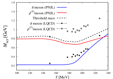
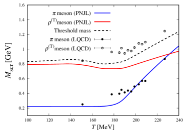
Fig. 1: $T$ dependence of ${M_{\pi}^{\rm scr}}(T)$ and ${M_{\pi}^{\rm scr}}(T)$. LQCD data (dots) are taken from Refs. Cheng:2010fe ; Maezawa:2016pwo . In the PNJL model, the Polyakov-loop potential taken is logarithmic-type in the upper panel, but polynomial-type in the lower panel. The vector coupling $G_{\rm V}(T)$ is independent of $T$. Note that $M_{\pi}^{\rm scr}(T)=M_{\pi}^{\rm pole}(T)$ at $T=0$. In the LQCD simulations, the $M_{\pi}^{\rm scr}(0)=220$ MeV is slightly heavier than the physical one ($M_{\pi}^{\rm pole}(0)=140$ MeV). We then change quark mass from $m_{0}=3.5$ MeV to $m_{0}=8.85$ MeV so as to reproduce $M_{\pi}^{\rm scr}(0)=220$ MeV. When we solve Eq. (49) for ${M_{\rho}^{\rm scr}}(T)$, the resulting ${M_{\rho}^{\rm scr}}(T)$ should be below the threshold mass $\mathcal{M}_{\rm lowest}$; see Eq. (68). The threshold mass (black-dots line) is always far below LQCD data on ${M_{\rho}^{\rm scr}}(T)$, indicating that the PNJL model does not reproduce the LQCD data.

As shown in the upper panel of Fig. 1, the PNJL model does not reproduce LQCD data Cheng:2010fe ; Maezawa:2016pwo on ${M_{\rho}^{\rm scr}}(T)$ above $T_{\rm c}^{\chi}\simeq T_{\rm c}^{\rm d}\approx 173$ MeV, when we take the logarithm-type Polyakov-loop potential $\mathcal{U}$ of Ref. Rossner et al. (2007). In the lower panel, we take the polynomial-type $\mathcal{U}$ (Poly-I) of Ref. Haas:2013qwp . The ${M_{\rho}^{\rm scr}}(T)$ for the polynomial-type $\mathcal{U}$ is better agreement with the corresponding LQCD data than that for the logarithm-type Polyakov-loop $\mathcal{U}$. From now on, we take the polynomial-type $\mathcal{U}$. The polynomial-type $\mathcal{U}$ reproduces the LQCD data for ${M_{\pi}^{\rm scr}}(T)$. Whenever we consider $\pi$, the mixing between $\pi$ and $A_{1}$ is taken into account. Finally we consider magnetic-gluon contribution on ${M_{\rho}^{\rm scr}}(T)$ and ${M_{\rho}^{\rm scr}}(T)$. The results are consistent with the LQCD data for ${M_{\rho}^{\rm scr}}(T)$ in $T>T_{\rm c}^{\rm d}$ and for ${M_{\pi}^{\rm scr}}(T)$ in both $T>T_{\rm c}^{\rm d}$ and $T<T_{\rm c}^{\rm d}$. We call the present version of PNJL model “magnetic-gluon (MG) PNJL”.

The MG-PNJL model is shown in Sec. II and numerical results are in Sec. III. Section IV is devoted to a summary.

II MG-PNJL model

In order to construct the MG-PNJL model, we consider the two-flavor case, since we focus on $\pi$, $\rho$ mesons in the case of finite $T$.

We start with the PNJL Lagrangian density with $T$-dependent scalar four-quark coupling $G_{\rm S}(T)$ and a constant vector coupling $G_{\rm V}(0)$: Namely,

$${\cal L} = {\bar{\psi}}(i\gamma_{\mu}D^{\mu}-m_{0})\psi+G_{\rm S}(T)[({\bar{\psi}}\psi)^{2}+({\bar{\psi}}i\gamma_{5}\bm{\tau}\psi)^{2}]$$

$$+ G_{\rm V}(0)\left[\left(\bar{\psi}\gamma^{\mu}\bm{\tau}\psi\right)^{2}+\left(\bar{\psi}\gamma^{\mu}\gamma_{5}\bm{\tau}\psi\right)^{2}\right]-{\cal U}(\Phi,{\bar{\Phi}},T),$$

(1)

where $\psi$ is the quark field with the current quark mass $m_{0}$, ${\vec{\tau}}$ stands for the isospin matrix. The covariant derivative $D^{\nu}$ is approximated into $\partial^{\nu}+\delta^{\nu}_{0}A^{0}_{a}{\lambda_{a}/2}$, where the time component $A_{a}^{0}$ of the gauge field is treated as a homogeneous and static background field governed by the Polyakov-loop potential $\mathcal{U}$. For $T$ dependence of $G_{\rm S}(T)$, we assume

$$G_{\rm S}(T)=\left\{\begin{array}[]{ll}G_{\rm S}(0)&(T<T_{\rm S})\\ G_{\rm S}(0)e^{-(T-T_{\rm S})^{2}/b_{\rm S}^{2}}&(T\geq T_{\rm S})\\ \end{array}\right..$$ (4)

As a Polyakov-loop potential $\mathcal{U}$, we consider two-types of $\mathcal{U}$. One is the logarithm-type potential of Ref. Rossner et al. (2007):

$$\frac{\mathcal{U}_{\rm log}(\Phi,\bar{\Phi},T)}{T^{4}} = -\frac{a(T)}{2}\Phi\bar{\Phi}+b(T){\rm ln}\left[1-6\Phi\bar{\Phi}\right.$$ (5)

$$\left.+4\left(\Phi^{3}+\bar{\Phi}^{3}\right)-3(\Phi\bar{\Phi})^{2}\right]$$

with

$$a(T)=a_{0}+a_{1}\left(\frac{T_{0}}{T}\right)+a_{2}\left(\frac{T_{0}}{T}\right)^{2},~{}~{}b(T)=b_{3}\left(\frac{T_{0}}{T}\right)^{3}$$ (6)

and another is the polynomial-type potential of Ref. Haas:2013qwp :

$$\frac{\mathcal{U}_{\rm poly}(\Phi,\bar{\Phi},T)}{T^{4}}=-\frac{b_{2}(T)}{2}\Phi\bar{\Phi}-\frac{b_{3}}{6}(\Phi^{3}+\bar{\Phi}^{3})+\frac{b_{4}}{4}(\Phi\bar{\Phi})^{2}$$ (7)

with

$$b_{2}(T)=c_{0}+c_{1}\left(\frac{T_{0}}{T}\right)+c_{2}\left(\frac{T_{0}}{T}\right)^{2}+c_{2}\left(\frac{T_{0}}{T}\right)^{3}$$ (8)

The parameters for each potential have been determined so as to reproduce thermodynamic quantities calculated with LQCD simulation in pure Yang–Mills theory. Their resultant values are summarized in Table 1. These potentials have one dimensionful parameter $T_{0}$. The value is $T_{0}=270$ MeV in pure Yang–Mills theory. Once one considers quark degree of freedom, the parameter $T_{0}$ should be shifted to a lower value in association with change of typical energy scale through the QCD running coupling $g$. Hence we treat $T_{0}$ as an adjustable parameter and determine to be consistent with full QCD data on the chiral temperature $T_{\rm c}\simeq 173$ MeV with 10% error Karsch, Leermann and Peikert (2002). The parameter thus obtained is $T_{0}=215$ MeV for each $\mathcal{U}$.

Table 1: Parameters taken in Polyakov-loop potentials

	$a_{0}$	$a_{1}$	$a_{2}$	$b_{3}$
Logarithm-type	3.51	-2.47	15.2	-1,75
	$b_{3}$	$b_{4}$	$c_{0}$	$c_{1}$	$c_{2}$	$c_{3}$
Polynomial-type	13.34	14.88	1.53	0.96	-2.3	-2.85

In the Polyakov gauge, the Polyakov-loop $\Phi$ and its conjugate ${\bar{\Phi}}$ are obtained by

$$\Phi ={1\over{3}}{\rm tr}_{\rm c}(L),~{}~{}~{}~{}~{}{\bar{\Phi}}={1\over{3}}{\rm tr}_{\rm c}({L^{*}})$$ (9)

with $L=\exp[iA_{4}/T]$ and $A_{4}/T={\rm diag}(\phi_{1},\phi_{2},\phi_{3})$ satisfying the condition that ${\phi}_{1}+{\phi}_{2}+{\phi}_{3}=0$. It is then possible to choice ${\phi}_{3}=0$ and determine the others from ${\phi}_{3}=0$. This leads to

$$\phi_{2}=-\phi_{1}=\cos^{-1}{\left(\frac{3\Phi-1}{2}\right)}.$$ (10)

Making the mean field approximation (MFA), one can get the MFA Lagrangian density as

$${\cal L}_{\rm MFA}={\bar{\psi}}S^{-1}\psi-U_{\rm M}(\sigma)-{\cal U}(\Phi,{\bar{\Phi}},T)$$ (11)

with the quark propagator

$$S=\frac{1}{i\gamma_{\mu}D^{\mu}-M}$$ (12)

for

$$M=m_{0}-2G_{\rm S}(T)\sigma,~{}U_{\rm M}=G_{\rm S}(T)\sigma^{2},~{}\sigma=\langle\bar{\psi}\psi\rangle.$$ (13)

We then obtain the thermodynamic potential $\Omega$ as

$$\Omega=U_{\rm M}+{\cal U}+\Omega_{\rm F}$$ (14)

with

$$\Omega_{\rm F} =-2N_{\rm c}N_{\rm f}\int\frac{d^{3}{\bm{p}}}{(2\pi)^{3}}\Bigl{[}E_{\bm{p}}$$

$$+\frac{T}{N_{\rm c}}\ln~{}[1+3(\Phi+{\bar{\Phi}}e^{-\beta E_{\bm{p}}})e^{-\beta E_{\bm{p}}}+e^{-3\beta E_{\bm{p}}}]$$

$$+\frac{T}{N_{\rm c}}\ln~{}[1+3({\bar{\Phi}}+{\Phi e^{-\beta E_{\bm{p}}}})e^{-\beta E_{\bm{p}}}+e^{-3\beta E_{\bm{p}}}]\Bigl{]}.$$ (15)

for $\beta=1/T$, $\Phi={\bar{\Phi}}$ and $E_{\bm{p}}=\sqrt{M+{\bm{p}}^{2}}$.

II.1 $\chi$-PV regularization

In Eq. (15), the momentum $\bm{p}$ integral has ultraviolet divergence and it must be regularized. As an usual regularization scheme, three-dimensional momentum cutoff has been commonly used so far, but the regularization explicitly breaks translational invariance that is essential for deriving the screening mass Ishii (2013). Moreover, translational invariance is also necessary to maintain Ward-Takahashi identities for $SU(2)_{\rm V}$ and $SU(2)_{\rm A}$ currents that realize transverse and longitudinal properties of $\rho$ and $A_{1}$ mesons. Hence we take a chiral version Ishii (2013) of Pauli-Villars (PV) regularization Pauli and Villars (1980); Florkowski (1997) in the present work. We refer to it as $\chi$-PV regularization. The original PV regularization cannot maintain chiral symmetry due to heavy masses of auxiliary particles, but $\chi$-PV regularization of Ref. Ishii (2013) manifestly preserves chiral symmetry and correctly reproduces low-energy relations of chiral dynamics, such as the Gell-Mann–Oakes–Renner relation, partial conserved axial-vector current relation and so on.

In $\chi$-PV regularization, the integral $\Omega_{\rm F}(M)$ is simply regularized as

$$\Omega_{\rm F}(M)\to\Omega^{\rm reg}_{\rm F}(M)=\sum_{\alpha=0}^{2}C_{\alpha}\Omega_{\rm F}(M_{\alpha})$$ (16)

with $M_{0}=M$ and the $M_{\alpha}~{}(\alpha\geq 1)$ are masses of auxiliary particles. The $M_{\alpha}$ and the $C_{\alpha}$ should satisfy the condition $\sum_{\alpha=0}^{2}C_{\alpha}=\sum_{\alpha=0}^{2}C_{\alpha}M_{\alpha}^{2}=0$ to remove the logarithmic, quadratic and quartic divergence. We then assume $(C_{0},C_{1},C_{2})=(1,-2,1)$ and $(M_{1}^{2},M_{2}^{2})=(M^{2}+\Lambda^{2},M^{2}+2\Lambda^{2})$. The dimensionful parameter $\Lambda$ should be kept to finite even after the subtraction (16), since the present model is non-renormalizable.

II.2 Parameter fitting

In the case of $T=0$ MeV, the present model has four parameters $m_{0},G_{\rm S}(0),G_{\rm V}(0)$ and the cutoff $\Lambda$. We fix the current quark mass $m_{0}$ to $3.5$ MeV, and determine the $G_{\rm S}(0),G_{\rm V}(0)$, $\Lambda$ from three realistic values of $M_{\pi}=140$ MeV, the pion decay constant $f_{\pi}=93.4$ MeV and $\rho$ meson mass $M_{\rho}=770$ MeV; see Table 2 for the values of $m_{0},\Lambda,G_{\rm S}(0)\Lambda^{2},G_{\rm V}(0)/G_{\rm S}(0)$.

Table 2: Model parameters in the NJL part.

$m_{0}$ [MeV]	$\Lambda$ [MeV]	$G_{\rm S}(0)\Lambda^{2}$	$G_{\rm V}(0)/G_{\rm S}(0)$
3.5	900	3.30	-1.36
$T_{\rm S}$ [MeV]	$b_{\rm S}$ [MeV]	$T_{0}$ [MeV]
135	115	215

For finite $T$, the present PNJL model with three adjustable parameters, i.e., $(T_{\rm S},b_{\rm S})$ in scalar-type coupling $G_{\rm S}(T)$ and a constant $T_{0}$ in the logarithm-type and the polynomial-type $\mathcal{U}$. These parameters are determined so as to reproduce LQCD data on $T$ dependence of chiral condensate $\sigma$; the chiral- and the deconfinement-transition temperature satisfy $T_{\rm c}^{\chi,{\rm LQCD}}=T_{\rm c}^{\rm d,LQCD}=173$ MeV within 10% errors Karsch, Leermann and Peikert (2002). The parameters thus obtained are $T_{0}=215$ MeV and $(T_{\rm S},b_{\rm S})=(135~{}{\rm MeV},115~{}{\rm MeV})$; Eventually, all the values shown in Table 2 are independent of the type of $\mathcal{U}$.

Figure 2 shows two cases of the logarithm-type and the polynomial-type $\mathcal{U}$. Comparing the solid line with the the corresponding dashed one for $\sigma/\sigma_{0}$, we find that $T$ dependence of $G_{\rm S}(T)$ is essential to explain the rapid decrease of $\sigma$ around $T=T_{\rm c}^{\chi,{\rm LQCD}}$ Karsch (2002); Karsch, Leermann and Peikert (2002).

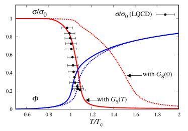
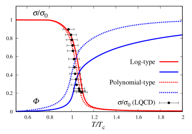
Fig. 2: $T$ dependence of the chiral condensate $\sigma$ and the Polyakov loop $\Phi$. The upper panel is results of the logarithm-type $\mathcal{U}$, while the lower panel is ones of the polynomial-type $\mathcal{U}$. The horizontal axis is scaled by $T_{\rm c}^{\chi}$. The chiral condensate is normalized by its value $\sigma_{0}$ at $T=0$. LQCD data are taken from Refs. Karsch (2002); Karsch, Leermann and Peikert (2002). The 10 % errors come from $T_{\rm c}^{\rm d,LQCD}$ and $T_{\rm c}^{\chi,{\rm LQCD}}$. In the upper panel, the solid lines denote the results of the present model with $T$-dependent $G_{\rm S}(T)$, whereas the dashed lines correspond to the results of the present model with a constant $G_{\rm S}(0)$.

II.3 Magnetic gluon contribution

Now we consider the Polynomial-type $\mathcal{U}$, since it yields better agreement with LQCD data on ${M_{\pi}^{\rm scr}}(T)$ and ${M_{\rho}^{\rm scr}}(T)$ than the logarithm-type one; see Fig. 1. In the PNJL model, magnetic gluon $\bm{A}^{a}(x)$ has been usually ignored, but the contribution should be important in the deconfinement phase $T>T_{\rm c}^{\rm d}$ Laine:2003bd . If one assumes the meson propagation into $z$-direction for convenience, the theory tells us that the ”electric” gluon field $A_{4}^{a}$ is totally canceled out by $z$-component of $\bm{A}^{a}$ and remaining $A_{x}^{a}$ and $A_{y}^{a}$ fields induce the positive mass-shift $C_{\rm F}/{8\pi}$ in the quark thermal mass $\mathcal{M}_{\rm thermal}$; namely,

$$\mathcal{M}_{\rm thermal}=\pi T+g_{\rm E}^{2}\frac{C_{\rm F}}{8\pi}+\mathcal{O}(g^{2}_{\rm E}/T)$$ (17)

with $C_{F}=(N_{\rm c}^{2}-1)/2N_{\rm c}$. We introduce effects of the shift with the replacement

$$\mathcal{M}_{j,n=0,\alpha}=\sqrt{M_{\alpha}^{2}+(\pi T+T\phi_{j})^{2}}\to\mathcal{M}_{\rm thermal},~{}~{}~{}$$ (18)

$$\mathcal{M}_{j,n=-1,\alpha}=\sqrt{M_{\alpha}^{2}+(-\pi T+T\phi_{j})^{2}}\to-\mathcal{M}_{\rm thermal}~{}~{}~{}~{}~{}$$ (19)

in $T>T_{\rm c}^{\rm d}$, although the other Matsubara frequencies $n$ are untouched. We have used $T$ dependence of gauge coupling $g_{\rm E}^{2}$ calculated with two-flavor up to two-loop order in Ref.  Laine:2003bd , where they optimize the scale parameter $\bar{\mu}$ and show $g_{\rm E}^{2}$ is less sensitive to variation around the optimized scale parameter $\bar{\mu}_{\rm opt}$; therefore we choose $\bar{\mu}=\bar{\mu}_{\rm opt}$ in the present calculation. The remaining parameter $\Lambda_{\bar{\rm MS}}$ should be related with typical energy scale of QCD. The ratio $\Lambda_{\bar{\rm MS}}/T_{\rm c}^{\rm d}$ has been estimated from LQCD data on zero temperature string tension or Sommer scale Laine:2003bd , and $\Lambda_{\bar{\rm MS}}/T_{\rm c}^{\rm d}$ has been almost equal to 1 within a few 10% error. Hence $\Lambda_{\bar{\rm MS}}\simeq T_{\rm c}^{\rm d}=173$ MeV is simply assumed here.

The PNJL result with the replacement is nothing but MG-PNJL model The MG-PNJL result (solid line) is shown in Fig. 3 for ${M_{\rho}^{\rm scr}}(T)$. The result is valid in $T>T_{\rm c}^{\rm d}$. Effects of the replacement are visible for ${M_{\pi}^{\rm scr}}(T)$. In a NJL-like model, we use the PNJL model with $G_{\rm S}(T)$ for $\Omega$ and set $\phi_{1}=\phi_{2}=\phi_{3}=0$ in Eqs. (49) and (65) for screening masses.

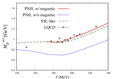
Fig. 3: $T$ dependence of transverse $\rho$-meson the Polynomial-type $\mathcal{U}$. The solid line stands for the result of MG-PNJL model. The dashed line denotes the result of the present PNJL model, while the dot-dashed line is a result of the NJL-like model that is explained in Sec. III.1.

III Numerical Results

III.1 The comparison with LQCD data

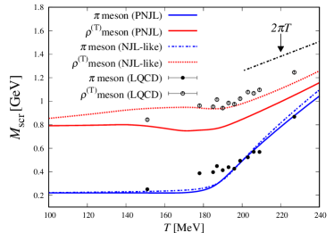
Fig. 4: $T$ dependence of $\pi$ and transverse $\rho$ mesons. with the Polynomial-type $\mathcal{U}$.

Figure 4 shows $\pi$ and $\rho$-meson screening masses calculated with PNJL and NJL-like models. For $\pi$ meson, the difference between PNJL and NJL-like results is tiny. The difference indicates that effects of $\phi_{i}$ are small for ${M_{\pi}^{\rm scr}}(T)$. For $\rho$ meson, the PNJL model agrees with LQCD data in the confinement phase $T<T_{\rm c}^{\rm d}=173$ MeV, but not in the deconfinement phases. The PNJL model shows mass reduction around $T\simeq T_{\rm c}^{\chi}$. This is attributed to decrease of effective-quark-mass $M$.

For transverse $\rho$ meson, the NJL-like result is above the PNJL one. Considering the consistency with LQCD data, one find that the PNJL model is more preferable than the NJL-like model in the confinement phase $T<T_{\rm c}^{\rm d}=173$ MeV. The failure of PNJL model in the deconfiment phase $T>T_{\rm c}^{\rm d}=173$ MeV comes from absence of magnetic gluon contribution, as shown in Fig. 4.

III.2 $T$ dependent of $G_{\rm V}$

Now we consider $T$ dependent of $G_{\rm V}(T)$ and assume the same form as $G_{\rm S}(T)$. As shown in Fig. 5, the $(T_{\rm V},b_{\rm V})$ controls $T$ dependence of the mass difference between $\pi$ and $\rho$ meson screening masses.

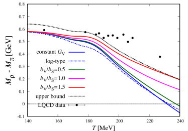
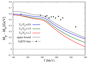
Fig. 5: Different sets of $(T_{\rm V},b_{\rm V})$. LQCD data are taken from Ref. Cheng:2010fe ; Maezawa:2016pwo .

IV Summary

We consider the two-flavor thermal system having $\mu=0$, and focus on $\pi$, $\rho$ mesons. As a model consistent with LQCD data on ${M_{\rho}^{\rm scr}}(T)$ and ${M_{\pi}^{\rm scr}}(T)$, we construct the MG-PNJLmodel. Whenever we consider $\pi$, the mixing between $\pi$ and $A_{1}$ is taken into account.

As shown in the upper panel of Fig. 1, the PNJL model does not reproduce LQCD data Cheng:2010fe ; Maezawa:2016pwo on ${M_{\rho}^{\rm scr}}(T)$ above $T_{\rm c}^{\chi}\simeq T_{\rm c}^{\rm d}\approx 173$ MeV, when we take the logarithm-type Polyakov-loop potential $\mathcal{U}$ of Ref. Rossner et al. (2007). In the lower panel, we take the polynomial-type $\mathcal{U}$ of Ref. Haas:2013qwp . The ${M_{\rho}^{\rm scr}}(T)$ for the polynomial-type $\mathcal{U}$ is better agreement with the corresponding LQCD data than that for the logarithm-type Polyakov-loop $\mathcal{U}$. We then took the polynomial-type $\mathcal{U}$. The polynomial-type $\mathcal{U}$ reproduces the LQCD data for ${M_{\pi}^{\rm scr}}(T)$. Finally we consider magnetic-gluon contribution on ${M_{\rho}^{\rm scr}}(T)$ and ${M_{\rho}^{\rm scr}}(T)$. The results are consistent with the LQCD data for ${M_{\rho}^{\rm scr}}(T)$ in $T>T_{\rm c}^{\rm d}$ and for ${M_{\pi}^{\rm scr}}(T)$ in both $T>T_{\rm c}^{\rm d}$ and $T<T_{\rm c}^{\rm d}$. The present version of PNJL model is referred to as “magnetic-gluon (MG) PNJL” in this paper.

Appendix A Meson screening mass

We derive the equation for $\pi$-, $\rho$- and $A_{1}$-meson screening masses by using the method of Refs. Ishii (2013).

The mesonic correlation function corresponding to $\pi,\rho,A_{1}$ meson is

$$J_{\xi}^{a}(x)=\bar{\psi}(x)\Gamma_{\xi}\tau^{a}\psi(x),\\$$

with matrices

$$\pi:~{}\Gamma_{\rm P}=i\gamma_{5},~{}~{}\rho:~{}\Gamma_{\rm V}=\gamma^{\mu},~{}~{}A_{1}:~{}\Gamma_{\rm A}=\gamma^{\mu}\gamma_{5}.$$ (20)

The mesonic correlation function is defined by

$$\eta_{\xi\xi^{\prime}}^{ab}(x)\equiv\langle 0|{\rm T}\left(J_{\xi}^{a}(x)J_{\xi^{\prime}}^{b}(0)\right)|0\rangle$$ (21)

and their Fourier transformed functions $\chi_{\xi\xi^{\prime}}^{ab}$ is then obtained by

$$\chi_{\xi\xi^{\prime}}^{ab}(q^{2})=i\int d^{4}xe^{iq\cdot x}\langle 0|{\rm T}\left(J_{\xi}^{a}(x)J_{\xi^{\prime}}^{b}(0)\right)|0\rangle.$$ (22)

where the indices $\xi,\xi^{\prime}$ means the $\pi,\rho,A_{1}$ channels as shown in (20) and T stands for the time ordered product. In the isospin symmetric case , mesonic correlation $\chi_{\xi\xi^{\prime}}^{ab}$ is simplified with $\delta^{ab}\chi_{\xi\xi^{\prime}}$; therefore, we abbreviate the indices $a,b$ unless otherwise stated.

The ring approximation in $\chi_{\xi\xi^{\prime}}$ leads to the Schwinger-Dyson equation

$$\chi_{\xi\xi^{\prime}}=\Pi_{\xi\xi^{\prime}}+\sum_{\xi^{\prime\prime}\xi^{\prime\prime\prime}}\Pi_{\xi\xi^{\prime\prime}}2G_{\xi^{\prime\prime}\xi^{\prime\prime\prime}}\chi_{\xi^{\prime\prime\prime}\xi^{\prime}},$$ (23)

where the one-loop polarization function $\Pi_{\xi\xi^{\prime}}$ is defined as

$$\Pi_{\xi\xi^{\prime}} \equiv -2i\int\frac{d^{4}p}{(2\pi)^{4}}{\rm tr}_{\rm c,d}\left[\Gamma_{\xi}iS(p^{\prime}+q)\Gamma_{\xi^{\prime}}iS(p^{\prime})\right]$$

with $p^{\prime}=(p_{0}+iA_{4},{\bm{p}})$ and trace ${\rm tr}_{\rm c,d}$ of color and Dirac spaces. We first consider the zero temperature case for simplicity. In this case, the polarization functions are summarized by

$$\mathit{\Pi}_{\rm PP} = -2i\int\frac{d^{4}p}{(2\pi)^{4}}{\rm tr}_{\rm c,d}\left[i\gamma_{5}iS(p^{\prime}+q)i\gamma_{5}iS(p^{\prime})\right]$$ (25)

$$\mathit{\Pi}_{\rm VV}^{\mu\nu} = -2i\int\frac{d^{4}p}{(2\pi)^{4}}{\rm tr}_{\rm c,d}\left[\gamma^{\mu}iS(p^{\prime}+q)\gamma^{\nu}iS(p^{\prime})\right]$$ (26)

$$\mathit{\Pi}_{\rm PA}^{\mu} = -2i\int\frac{d^{4}p}{(2\pi)^{4}}{\rm tr}_{\rm c,d}\left[i\gamma_{5}iS(p^{\prime}+q)\gamma^{\mu}\gamma_{5}iS(p^{\prime})\right]$$ (27)

$$\mathit{\Pi}_{\rm AP}^{\mu} = -2i\int\frac{d^{4}p}{(2\pi)^{4}}{\rm tr}_{\rm c,d}\left[\gamma^{\mu}\gamma_{5}iS(p^{\prime}+q)i\gamma_{5}iS(p^{\prime})\right]$$ (28)

$$\mathit{\Pi}_{\rm AA}^{\mu\nu} = -2i\int\frac{d^{4}p}{(2\pi)^{4}}{\rm tr}_{\rm c,d}\left[\gamma^{\mu}\gamma_{5}iS(p^{\prime}+q)\gamma^{\nu}\gamma_{5}iS(p^{\prime})\right].$$

Taking the trace ${\rm tr}_{\rm d}$ of Dirac index, we obtain the explicit form of polarization functions:

$$\mathit{\Pi}_{\rm PP} = 8I_{1}-4q^{2}I_{2}$$ (30)

$$\mathit{\Pi}_{\rm PA}^{\mu} = -\mathit{\Pi}_{\rm AP}^{\mu}=8iMq^{\mu}I_{2}.$$ (31)

for psedoscalar and $\pi$-$A_{1}$ mixing channel, where the functions $I_{!}$ and $I_{2}$ is represented by

$$I_{1} = i{\rm tr_{c}}\int{d^{4}p\over{(2\pi)^{4}}}{1\over{p^{\prime 2}-M^{2}}+i\epsilon},$$ (32)

$$I_{2} = i{\rm tr_{c}}\int{d^{4}p\over{(2\pi)^{4}}}{1\over{\{(p^{\prime}+q)^{2}-M^{2}+i\epsilon\}(p^{\prime 2}-M^{2}+i\epsilon)}},$$

see Appendix for momentum $p$-integrated form of $I_{1}$ and $I_{2}$. In the vector and axial-vector channel, $\Pi_{\rm VV}^{\mu\nu}$ and $\Pi_{\rm AA}^{\mu\nu}$ are represented by

$$\mathit{\Pi}_{\rm VV}^{\mu\nu} = -8i{\rm tr}_{\rm c}\int\frac{d^{4}p}{(2\pi)^{4}}$$

$$\frac{2p^{\prime\mu}p^{\prime\nu}-q^{\mu}q^{\nu}/2-\left(p^{\prime 2}-q^{2}/4-M^{2}\right)g^{\mu\nu}}{\left\{(p^{\prime}+q/2)^{2}-M^{2}+i\epsilon\right\}\left\{(p^{\prime}-q/2)^{2}-M^{2}+i\epsilon\right\}},$$

$$\mathit{\Pi}_{\rm AA}^{\mu\nu} = \mathit{\Pi}_{\rm VV}^{\mu\nu}-16M^{2}I_{2}g^{\mu\nu}$$ (35)

The extension to finite $T$ case can be made by following replacement:

$$p_{0}\to i\omega_{n}=i(2n+1)\pi T,$$

$$\int\frac{d^{4}p}{(2\pi)^{4}}\to iT\sum_{n=-\infty}^{\infty}\int\frac{d^{3}p}{(2\pi)^{3}}.$$ (36)

One can then obtain PV regularized functions $I_{1}^{\rm reg},I_{2}^{\rm reg}$ at finite $T$ in the static limit as

$$I_{1}^{\rm reg} = T\sum_{j,n,\alpha}\int{d^{3}\bm{p}\over{(2\pi)^{3}}}C_{\alpha}{1\over{\bm{p}^{2}+\mathcal{M}_{j,n,\alpha}^{2}}}$$ (37)

$$I_{2}^{\rm reg} = -T\sum_{j,n,\alpha}\int{d^{3}\bm{p}\over{(2\pi)^{3}}}C_{\alpha}{1\over{(\bm{p+q})^{2}+\mathcal{M}_{j,n,\alpha}^{2}}}{1\over{\bm{p}^{2}+\mathcal{M}_{j,n,\alpha}^{2}}}$$

with the summation $\sum_{j,n,\alpha}=\sum_{j=1}^{N_{\rm c}}\sum_{n=-\infty}^{\infty}\sum_{\alpha=0}^{2}$, where the summation $\sum_{\alpha=0}^{2}$ should be taken before the summation $\sum_{n=-\infty}^{\infty}$ and $\bm{p}$-integral for convergence. The mass $\mathcal{M}_{j,n,\alpha}$ depends on temperature and phase $\phi_{j}$ as

$$\mathcal{M}_{j,n,\alpha}=\sqrt{M_{\alpha}^{2}+(\omega_{n}+T\phi_{j})^{2}}.$$ (39)

We mention $\mathcal{M}_{j,n,\alpha}$ as ”thermal quark mass” since $\mathcal{M}_{j,n,\alpha}$ acts as (chiral symmetric) quark mass in 3-dimensional momentum $\bm{p}$ space of Eqs. (37) and (LABEL:I2_tem) .

Appendix B $\rho$ and $A_{1}$ meson screening masses at finite $T$

In this section, we only consider the $\xi={\rm V,\rm A}$ channels. At zero temperature, the polarization functions $\mathit{\Pi}_{\xi\xi}^{\mu\nu}$ and mesonic correlation $\chi_{\xi\xi}^{\mu\nu}$ are decomposed into 4-dimensionally transverse and longitudinal modes:

$$\mathit{\Pi}_{\xi\xi}^{\mu\nu} = \mathit{\Pi}_{\xi\xi}^{({\rm T,4d})}T^{\mu\nu}+\mathit{\Pi}_{\xi\xi}^{({\rm L,4d})}L^{\mu\nu}$$

$$\chi_{\xi\xi}^{\mu\nu} = \chi_{\xi\xi}^{({\rm T,4d})}T^{\mu\nu}+\chi_{\xi\xi}^{({\rm L,4d})}L^{\mu\nu}$$ (40)

The projection tensors $T^{\mu\nu}$ and $L^{\mu\nu}$ are defined by

$$T^{\mu\nu}=g^{\mu\nu}-\frac{q^{\mu}q^{\nu}}{q^{2}},~{}~{}L^{\mu\nu}=\frac{q^{\mu}q^{\nu}}{q^{2}}.$$ (41)

It is noted that the longitudinal element $\Pi_{\rm VV}^{({\rm L,4d})}$ must vanish due to isospin symmetry since the isovector current should be conserved ($\partial_{\mu}J_{\rm V}^{\mu a}(x)=0$) and the corresponding Ward-Takahashi identity indicates $q_{\mu}\Pi_{\rm VV}^{\mu\nu}=0$ and $q_{\mu}\chi_{\rm VV}^{\mu\nu}=0$. The vanishment of $\Pi_{\rm VV}^{({\rm L,4d})}$ and $\Pi_{\rm VV}^{({\rm L,4d})}$ is realized even at finite $T$ because the current conservation law holds for any $T$. If one chooses three-dimensional momentum-cutoff regularization, the Ward-Takahashi identity is spoiled and the above discussion is no longer valid due to the lack of translational invariance.

At finite $T$, the 4-dimensionally transverse mode is decomposed into 3-dimensionally transverse and longitudinal modes in the polarization function and mesonic correlation:

$$\mathit{\Pi}_{\xi\xi}^{\mu\nu} = \mathit{\Pi}_{\xi\xi}^{({\rm T,3d})}P^{\mu\nu}_{\rm T}+\mathit{\Pi}_{\xi\xi}^{({\rm L,3d})}P^{\mu\nu}_{\rm L}+\mathit{\Pi}_{\xi\xi}^{({\rm L,4d})}L^{\mu\nu},$$

$$\chi_{\xi\xi}^{\mu\nu} = \chi_{\xi\xi}^{({\rm T,3d})}P^{\mu\nu}_{\rm T}+\chi_{\xi\xi}^{({\rm L,3d})}P^{\mu\nu}_{\rm L}+\chi_{\xi\xi}^{({\rm L,4d})}L^{\mu\nu}.$$ (42)

The 3-dimensional projection tensors are defined by

$$P^{\mu\nu}_{\rm T}=g^{\mu\nu}-\frac{q^{\mu}q^{\nu}}{q^{2}}-\frac{n^{\mu}n^{\nu}}{n^{2}},~{}~{}P^{\mu\nu}_{\rm L}=\frac{n^{\mu}n^{\nu}}{n^{2}},$$ (43)

where the 4-dimensional vector $n^{\mu}$ is orthogonal component of heat bath velocity $u^{\mu}$ against the external momentum $q^{\mu}$, i.e., $n^{\mu}=T^{\mu\nu}u_{\nu}$. When one takes the rest frame of heat bath ($u^{\mu}=(1,\bm{0})$) and the static limit, the vector $n^{\mu}$ turns out to be equal to $u^{\mu}$. The general discussion of projection tensor is summarized in Appendix.

In the SD equation (23), 3-dimensionally transverse and longitudinal modes has been completely decoupled, and one can independently solve the equations for each modes. The solution of SD equation is finally obtained as

$$\chi_{\xi\xi}^{({\rm T,3d})}=\frac{\Pi_{\xi\xi}^{({\rm T,3d})}}{1-2G_{\rm V}\Pi_{\xi\xi}^{({\rm T,3d})}},~{}~{}\chi_{\xi\xi}^{({\rm L,3d})}=\frac{\Pi_{\xi\xi}^{({\rm L,3d})}}{1-2G_{\rm V}\Pi_{\xi\xi}^{({\rm L,3d})}}$$

for $\xi={\rm A},{\rm V}$. The polarization functions are simple form

$$\Pi_{\rm VV}^{({\rm T,3d})} = -16\bm{q}^{2}I_{3}^{\rm reg},~{}~{}\Pi_{\rm AA}^{({\rm T,3d})}=-16\bm{q}^{2}I_{3}^{\rm reg}-16M^{2}I_{2}^{\rm reg},$$

$$\Pi_{\rm VV}^{({\rm L,3d})} = -16I_{4}^{\rm reg},~{}~{}\Pi_{\rm AA}^{({\rm L,3d})}=-16I_{4}^{\rm reg}-16M^{2}I_{2}^{\rm reg},$$ (45)

where the functions $I_{3}^{\rm reg}$ and $I_{4}^{\rm reg}$ are

$$I_{3}^{\rm reg} = -T\sum_{j,n,\alpha}\int{d^{3}\bm{p}\over{(2\pi)^{3}}}\int_{0}^{1}dx~{}C_{\alpha}{x-x^{2}\over{\bm{p}^{2}+\mathcal{M}^{2}_{j,n,\alpha}(\bm{q}^{2})}}$$

$$I_{4}^{\rm reg} = \bm{q}^{2}I_{3}^{\rm reg}-T\sum_{j,n,\alpha}\int{d^{3}\bm{p}\over{(2\pi)^{3}}}\int_{0}^{1}dx~{}C_{\alpha}{\omega_{n}^{{}^{\prime}2}-\bm{p}^{2}/3\over{\bm{p}^{2}+\mathcal{M}^{2}_{j,n,\alpha}(\bm{q}^{2})}}$$

with $\omega_{n}^{\prime}=\omega_{n}+\phi_{j}$, Feynman parameter $x$ and $\mathcal{M}^{2}_{j,n,\alpha}(\bm{q}^{2})=\mathcal{M}^{2}_{j,n,\alpha}+(x-x^{2})\bm{q}^{2}$. It is worth noting that the Feynman parameter must be carefully taken in thermal field theory, since the naive treatment of Feynman parameter leads to wrong results due to ambiguity of the analytic continuation from the Euclid space to the Minkowski space. In the present case, the all calculation has been done in the Euclid space and such a difficulty does not arise.

The $\rho$- and $A_{1}$-meson screening masses are obtained by searching the pole position of the denominator:

$$\left.\left[{1-2G_{\rm V}\Pi_{\xi\xi}^{({\rm T,3d})}}\right]\right|_{\tilde{q}=iM_{\rho}^{\rm scr}~{}{\rm or}~{}iM_{A_{1}}^{\rm scr}} = 0$$ (48)

$$\left.\left[{1-2G_{\rm V}\Pi_{\xi\xi}^{({\rm L,3d})}}\right]\right|_{\tilde{q}=iM_{\rho}^{\rm scr}~{}{\rm or}~{}iM_{A_{1}}^{\rm scr}} = 0$$ (49)

with $\tilde{q}=|\bm{q}|$.

B.1 $\pi$ meson screening mass with $\pi-A_{1}$ mixing

The $\pi$ meson is coupled with 4-dimensionally longitudinal mode of $A_{1}$ meson; therefore, the SD equation becomes coupled channel equation:

$$\chi_{\rm PP} = \mathit{\Pi}_{\rm PP}+\mathit{\Pi}_{\rm PP}2G_{\rm S}\chi_{\rm PP}+\bar{\mathit{\Pi}}_{\rm PA}2G_{\rm V}\bar{\chi}_{\rm AP}$$ (50)

$$\bar{\chi}_{\rm AP} = \bar{\mathit{\Pi}}_{\rm AP}+\bar{\mathit{\Pi}}_{\rm AP}2G_{\rm S}\chi_{\rm PP}+\mathit{\Pi}_{\rm AA}^{({\rm L,4d})}2G_{\rm V}\bar{\chi}_{\rm AP}$$ (51)

$$\bar{\chi}_{\rm PA} = \bar{\mathit{\Pi}}_{\rm PA}+\bar{\mathit{\Pi}}_{\rm PA}2G_{\rm V}\chi_{\rm AA}^{({\rm L,4d})}+\mathit{\Pi}_{\rm PP}2G_{\rm S}\bar{\chi}_{\rm PA}$$ (52)

$$\chi_{\rm AA}^{({\rm L,4d})} = \mathit{\Pi}_{\rm AA}^{({\rm L,4d})}+\mathit{\Pi}_{\rm AA}^{({\rm L,4d})}2G_{\rm V}\chi_{\rm AA}^{({\rm L,4d})}+\bar{\mathit{\Pi}}_{\rm AP}2G_{\rm S}\bar{\chi}_{\rm PA}$$

For convenience, the pseudoscalar-axialvector mixing channels $\chi_{\rm AP}^{\mu},\chi_{\rm PA}^{\mu},\Pi_{\rm AP}^{\mu},\Pi_{\rm PA}^{\mu}$ are rewritten by $\bar{\chi}_{\rm AP(PA)}=\hat{q}_{\mu}\chi_{\rm AP(PA)}^{\mu},\bar{\Pi}_{\rm AP(PA)}=\hat{q}_{\mu}\Pi_{(\rm AP)PA}^{\mu}$ with unit vector $\hat{q}^{\mu}=q^{\mu}/\sqrt{q^{2}}$. When one introduces the following matrices,

$$\bm{\chi} = \left(\begin{array}[]{cc}\chi_{\rm PP}&\bar{\chi}_{\rm PA}\\ \bar{\chi}_{\rm AP}&\chi_{\rm AA}^{({\rm L,4d})}\end{array}\right),~{}~{}\bm{G}=\left(\begin{array}[]{cc}G_{\rm S}&0\\ 0&G_{\rm V}\end{array}\right)$$ (58)

$$\bm{\mathit{\Pi}} = \left(\begin{array}[]{cc}\mathit{\Pi}_{\rm PP}&\bar{\mathit{\Pi}}_{\rm PA}\\ \bar{\mathit{\Pi}}_{\rm AP}&\mathit{\Pi}_{\rm AA}^{({\rm L,4d})}\end{array}\right),$$ (61)

the solution of SD equation is easily found as

$$\bm{\chi}=\frac{\tilde{\bm{\mathit{\Pi}}}\bm{\mathit{\Pi}}}{\det{\left[\bm{I}-2\bm{\mathit{\Pi}}\bm{G}\right]}}.$$ (62)

The matrix $\tilde{\bm{\mathit{\Pi}}}$ is

$$\tilde{\bm{\mathit{\Pi}}}=\left(\begin{array}[]{cc}1-2G_{\rm V}\mathit{\Pi}_{\rm AA}^{({\rm L,4d})}&2G_{\rm V}\bar{\mathit{\Pi}}_{\rm PA}\\ 2G_{\rm S}\bar{\mathit{\Pi}}_{\rm AP}&1-2G_{\rm S}\mathit{\Pi}_{\rm PP}\end{array}\right)$$ (63)

and the determinant is

$$\det{\left[\bm{I}-2\bm{\mathit{\Pi}}\bm{G}\right]} = \left(1-2G_{\rm S}\mathit{\Pi}_{\rm PP}\right)\left(1-2G_{\rm V}\mathit{\Pi}_{\rm AA}^{({\rm L,4d})}\right)$$ (64)

$$- 4G_{\rm S}G_{\rm V}\bar{\mathit{\Pi}}_{\rm AP}\bar{\mathit{\Pi}}_{\rm PA}.$$

The $\pi$ meson screening mass is then obtained by

$$\left.\det{\left[\bm{I}-2\bm{\mathit{\Pi}}\bm{G}\right]}\right|_{\tilde{q}=iM_{\xi}^{\rm scr}}=0$$ (65)

for $\xi=\pi$ meson and $A_{1}$ meson in 4-dimensionally longitudinal state. We numerically found that any pole since .

Appendix C Threshold mass

In PNJL model, mesons can decay into quark-pair. Such a effect is emerged in the functions $I_{2},I_{3},I_{4}$:

$$I_{2}^{\rm reg} = \frac{iT}{8\pi\tilde{q}}{\rm Log}{\left(\frac{2\mathcal{M}_{j,n,\alpha}+i\tilde{q}}{2\mathcal{M}_{j,n,\alpha}-i\tilde{q}}\right)}$$

$$I_{3}^{\rm reg} = \frac{iT}{64\pi\tilde{q}}\sum_{j,n,\alpha}\left[\left(1-\frac{4\mathcal{M}_{j,n,\alpha}^{2}}{\tilde{q}^{2}}\right){\rm Log}{\left(\frac{2\mathcal{M}_{j,n,\alpha}+i\tilde{q}}{2\mathcal{M}_{j,n,\alpha}-i\tilde{q}}\right)}\right.$$

$$+ \left.\frac{4i\mathcal{M}_{j,n,\alpha}}{\tilde{q}}\right]$$

$$I_{4}^{\rm reg} = \frac{i\tilde{q}T}{32\pi}\sum_{j,n,\alpha}\left[\left(1+\frac{4\omega_{n}^{2}}{\tilde{q}^{2}}\right){\rm Log}{\left(\frac{2\mathcal{M}_{j,n,\alpha}+i\tilde{q}}{2\mathcal{M}_{j,n,\alpha}-i\tilde{q}}\right)}\right.$$ (67)

$$+ \left.\frac{4i\mathcal{M}_{j,n,\alpha}}{\tilde{q}}\right],$$

as logarithmic cuts along the imaginary axis in complex $\tilde{q}$ plane, where logarithmic cuts are starting at $\tilde{q}=2i\mathcal{M}_{j,n,\alpha}$ and lowest branch point is given by $\tilde{q}=i\mathcal{M}_{\rm lowest}$ with

$$\mathcal{M}_{\rm lowest}=2\mathcal{M}_{j=1,n=0,\alpha=0}=2\mathcal{M}_{j=2,n=-1,\alpha=0}.$$ (68)

When $\tilde{q}\geq i\mathcal{M}_{\rm lowest}$, meson decays into quark-pair. The $\mathcal{M}_{\rm lowest}$ is thus ”threshold mass”.

PNJL model describes statistical confinement by means of Polyakov loop, but has no information about the confinement force between quarks because the gauge fields are treated as background field and their nonlocal correlations are ignored. Accordingly, PNJL model may be less predictive to meson screening mass above the threshold mass. Hence we assume that our model results are reliable only when the following relation is satisfied:

$$M_{\xi}^{\rm scr}<\mathcal{M}_{\rm lowest}$$ (69)

for $\xi=\pi,\rho,A_{1}$ mesons.

References

(1)
M. Cheng, S. Datta, A. Francis, J. van der Heide, C. Jung, O. Kaczmarek, F. Karsch and E. Laermann et al.,
Eur. Phys. J. C 71, 1564 (2011)
[arXiv:1010.1216 [hep-lat]].
(2)
Y. Maezawa, F. Karsch, S. Mukherjee and P. Petreczky,
PoS LATTICE 2015, 199 (2016).
(3)
C. Song,
Phys. Rev. D 48, 1375 (1993).
(4)
Y. B. He, J. Hufner, S. P. Klevansky and P. Rehberg,
Nucl. Phys. A 630, 719 (1998)
(5)
D. Blaschke, G. Burau, M. K. Volkov and V. L. Yudichev,
Eur. Phys. J. A 11, 319 (2001).
Meisinger et al. (1996)
P. N. Meisinger,
and
M. C. Ogilvie,
Phys. Lett. B 379,
163 (1996).
Dumitru (2002)
A. Dumitru,
and
R. D. Pisarski,
Phys. Rev. D 66,
096003 (2002).
Fukushima (2004)
K. Fukushima,
Phys. Lett. B 591,
277 (2004);
K. Fukushima,
Phys. Rev. D 77,
114028 (2008);
Phys. Rev. D 78,
114019 (2008).
Costa (2005)
P. Costa,
M. C. Ruivo,
C. A. de Sousa,
and
Yu. L. Kalinovsky,
Phys. Rev. D 71,
116002 (2005).
S. K. Ghosh et al. (2006)
S. K. Ghosh,
T. K. Mukherjee,
M. G. Mustafa, and
R. Ray,
Phys. Rev. D 73,
114007 (2006).
Megias et al. (2006)
E. Megas,
E. R. Arriola,
and
L. L. Salcedo,
Phys. Rev. D 74,
065005 (2006).
Ratti et al. (2006)
C. Ratti,
M. A. Thaler,
and
W. Weise,
Phys. Rev. D 73,
014019 (2006).
Ciminale (2007)
M. Ciminale,
R. Gatto,
G. Nardulli,
and
M. Ruggieri,
Phys. Lett. B 657,
64 (2007);
M. Ciminale,
R. Gatto,
N. D. Ippolito,
G. Nardulli,
and
M. Ruggieri,
Phys. Rev. D 77,
054023 (2008).
Ratti et al. (2007)
C. Ratti,
S. Rößner,
M. A. Thaler,
and
W. Weise,
Eur. Phys. J. C 49,
213 (2007).
Rossner et al. (2007)
S. Rößner,
C. Ratti,
and
W. Weise,
Phys. Rev. D 75,
034007 (2007).
Hansen et al. (2007)
H. Hansen,
W. M. Alberico,
A. Beraudo,
A. Molinari,
M. Nardi,
and
C. Ratti,
Phys. Rev. D 75,
065004 (2007).
Sasaki et al. (2007)
C. Sasaki,
B. Friman,
and
K. Redlich,
Phys. Rev. D 75,
074013 (2007).
Schaefer (2007)
B. -J. Schaefer,
J. M. Pawlowski,
and
J. Wambach,
Phys. Rev. D 76,
074023 (2007).
Kashiwa et al (2008)
K. Kashiwa,
H. Kouno,
M. Matsuzaki,
and
M. Yahiro,
Phys. Lett. B 662,
26 (2008).
(20)
Y. Sakai, K. Kashiwa, H. Kouno, and M. Yahiro,
Phys. Rev. D 77, 051901(R) (2008);
78, 036001 (2008).
(21)
Y. Sakai, K. Kashiwa, H. Kouno, M. Matsuzaki,
and M. Yahiro,
Phys. Rev. D 78, 076007 (2008);
79, 096001 (2009).
(22)
Y. Sakai, T. Sasaki, H. Kouno, and M. Yahiro,
J. Phys. G 37, 105007 (2010).
Costa (2009)
P. Costa,
M. C. Ruivo,
C. A. de Sousa,
H. Hansen,
and
W. M. Alberico,
Phys. Rev. D 79,
116003 (2009).
Ruivo (2012)
M. C. Ruivo,
M. Santos.,
P. Costa,
and
C. A. de Sousa,
Phys. Rev. D 85,
036001 (2012).
(25)
Y. Sakai, T. Sasaki, H. Kouno and M. Yahiro,
Phys. Rev. D 82, 076003 (2010).
Sasaki et al. (2009)
T. Sasaki,
Y. Sakai,
H. Kouno,
and
M. Yahiro,
Phys. Rev. D
84,
091901 (2011).
Florkowski (1997)
W. Florkowski,
Acta Phys. Pol. B 28,
2079 (1997).
Ishii (2013)
M. Ishii,
T. Sasaki,
K. Kashiwa,
H. Kouno,
and
M. Yahiro,
Phys. Rev. D
89,
071901(R) (2014).
Ishii (2015)
M. Ishii,
K. Yonemura,
J. Takahashi,
H. Kouno,
and
M. Yahiro,
Phys. Rev. D
93,
016002 (2016).
(30)
M. Ishii, H. Kouno and M. Yahiro,
Phys. Rev. D 95, 114022 (2017)
(31)
M. Ishii, A. Miyahara, H. Kouno and M. Yahiro,
Phys. Rev. D 99, no.11, 114010 (2019).
(32)
L. M. Haas, R. Stiele, J. Braun, J. M. Pawlowski and J. Schaffner-Bielich,
Phys. Rev. D 87, no.7, 076004 (2013)
doi:10.1103/PhysRevD.87.076004
[arXiv:1302.1993 [hep-ph]].
Karsch, Leermann and Peikert (2002)
F. Karsch,
E. Laermann,
and
A. Peikert,
Nucl. Phys. B 605,
579 (2002).
Pauli and Villars (1980)
W. Pauli,
and
F. Villars,
Rev. Mod. Phys. 21,
434 (1949).
Karsch (2002)
F. Karsch,
Lect. notes Phys. 583,
209 (2002).
(36)
M. Laine and M. Vepsalainen,
JHEP 02, 004 (2004).