Cost efficiency of institutional incentives in finite populations

Abstract

Institutions can provide incentives to increase cooperation behaviour in a population where this behaviour is infrequent. This process is costly, and it is thus important to optimize the overall spending. This problem can be mathematically formulated as a multi-objective optimization problem where one wishes to minimize the cost of providing incentives while ensuring a desired level of cooperation within the population. In this paper, we provide a rigorous analysis for this problem. We study cooperation dilemmas in both the pairwise (the Donation game) and multi-player (the Public Goods game) settings. We prove the regularity of the (total incentive) cost function, characterize its asymptotic limits (infinite population, weak selection and large selection) and show exactly when reward or punishment is more efficient. We prove that the cost function exhibits a phase transition phenomena when the intensity of selection varies. We calculate the critical threshold in regards to the phase transition and study the optimization problem when the intensity of selection is under and above the critical value. It allows us to provide an exact calculation for the optimal cost of incentive, for a given intensity of selection. Finally, we provide numerical simulations to demonstrate the analytical results. Overall, our analysis provides for the first time a selection-dependent calculation of the optimal cost of institutional incentives (for both reward and punishment) that guarantees a minimum amount of cooperation. It is of crucial importance for real-world applications of institutional incentives since intensity of selection is specific to a given population and the underlying game payoff structure.

Key words: institution, incentives, cost optimization, evolutionary game theory, evolution of cooperation.

1 Introduction

The problem of promoting the evolution of cooperative behaviour within populations of self-regarding individuals has been intensively investigated across diverse fields of behavioural, social and computational sciences (Perc et al., 2017; Nowak, 2006b; Han, 2013; West et al., 2007; Sigmund, 2010). Various mechanisms responsible for promoting the emergence and stability of cooperative behaviours among such individuals have been proposed. They include kin and group selection (Hamilton, 1964; Traulsen and Nowak, 2006), direct and indirect reciprocities  (Ohtsuki and Iwasa, 2006; Krellner and Han, 2020; Nowak and Sigmund, 2005; Han et al., 2012; Okada, 2020), spatial networks (Santos et al., 2006; Perc et al., 2013; Antonioni and Cardillo, 2017; Peña et al., 2016), reward and punishment  (Fehr and Gachter, 2000; Boyd et al., 2003; Sigmund et al., 2001; Herrmann et al., 2008; Hauert et al., 2007a; Boyd et al., 2010), and pre-commitments (Nesse, 2001; Han et al., 2013; Martinez-Vaquero et al., 2017; Han et al., 2016; Sasaki et al., 2015). Institutional incentives, namely, rewards for cooperation and punishment of wrongdoing, are among the most important ones (Wang et al., 2019; Sigmund et al., 2001; Han and Tran-Thanh, 2018; Sigmund et al., 2010; Vasconcelos et al., 2013; Chen et al., 2015; Wu et al., 2014; García and Traulsen, 2019; Góis et al., 2019; Powers et al., 2018). Differently from other mechanisms, in order to carry out institutional incentives, it is assumed that there exists an external decision maker (e.g. institutions such as the United Nations and the European Union) that has a budget to interfere in the population to achieve a desirable outcome. Institutional enforcement mechanisms are crucial for enabling large-scale cooperation. Most modern societies implemented different forms of institutions for governing and promoting collective behaviors, including cooperation, coordination, and technology innovation (Ostrom, 1990; Bowles, 2009; Bowles and Gintis, 2002; Bardhan, 2005; Han et al., 2021; Scotchmer, 2004).

Providing incentives is costly and it is important to minimize the cost while ensuring a sufficient level of cooperation (Ostrom, 1990; Chen et al., 2015; Han and Tran-Thanh, 2018). Despite of its paramount importance, so far there have been only few works exploring this question. In particular, Wang et al. (2019) use optimal control theory to provide an analytical solution for cost optimization of institutional incentives assuming deterministic evolution and infinite population sizes (modeled using replicator dynamics). This work therefore does not take into account various stochastic effects of evolutionary dynamics such as mutation and non-deterministic behavioral update (Traulsen et al., 2006; Sigmund, 2010; Hofbauer and Sigmund, 1998). Defective behaviour can reoccur over time via mutation or when incentives were not strong or effective enough in the past, requiring institutions to spend more budget on providing incentive. Moreover, a key factor of behavioral update, the intensity of selection (Sigmund, 2010)—which determines how strongly an individual bases her decision to copy another individual’s strategy on fitness difference—might strongly impact an institutional incentives strategy and its cost efficiency. For instance, when selection is weak such that behavioral update is close to a random process (i.e. an imitation decision is independent of how large the fitness difference is), providing incentives would make little difference to cause behavioral change, however strong it is. When selection is strong, incentives that ensure a minimum fitness advantage to cooperators would already ensure positive behavioral change.

In a stochastic, finite population context, so far this problem has been investigated primarily based on agent-based and numerical simulations (Chen et al., 2015; Sasaki et al., 2012; Han et al., 2018; Han and Tran-Thanh, 2018; Cimpeanu et al., 2019). Results demonstrate several interesting phenomena, such as the significant influence of the intensity of selection on incentive strategies and optimal costs. However, there is no satisfactory rigorous analysis available at present that allows one to derive the optimal way of providing incentives (for a given cooperation dilemma and desired level of cooperation). This is a challenging problem because of the large but finite population size and the complexity of stochastic processes on the population.

In this paper, we provide exactly such a rigorous analysis. We study cooperation dilemmas in both pairwise (the donation game) and multi-player (the Public Goods game) settings. These are the most studied models for studying cooperation where individually defection is always preferred over cooperation while mutual cooperation is the preferred collective outcome for the population as a whole. Adopting a popular stochastic evolutionary game approach for analysing well-mixed finite populations (Nowak et al., 2004; Imhof et al., 2005; Nowak, 2006a), we derive the total expected costs of providing institutional reward or punishment, characterize their asymptotic limits (infinite population, weak selection and large selection) and show the existence of a phase transition phenomena in the optimization problem when the intensity of selection varies. We calculate the critical threshold of phase transitions and study the minimization problem when the intensity of selection is under and above the critical value. We furthermore provide numerical simulations to demonstrate the analytical results.

The rest of the paper is organized as follows. In Section 2 we introduce the models and methods deriving mathematical optimization problems that will be studied. The main results of the paper are presented in Section 3. In Section 4 we give explicit computations for small populations and numerical investigations demonstrating the analytical results. In Section 5 we discuss possible extensions for future work. Finally, detailed computations, technical lemmas and proofs the main results are provided in the Supplementary Information attached at the end of the paper.

2 Materials and Methods

2.1 Cooperation dilemmas

We consider a well-mixed, finite population of $N$ self-regarding individuals or players, who interact with each other using one of the following cooperation dilemmas, namely the Donation Game (DG) and the Public Goods Game (PGG). Let $\Pi_{C}(i)$ and $\Pi_{D}(i)$ denote the payoffs of Cooperator (C) and Defector (D) in a population with $i$ C players and $N-i$ D players. We show below that $\Pi_{C}(i)-\Pi_{D}(i)$ is a constant, which is denoted by $\delta$. For cooperation dilemmas, it’s always the case that $\delta<0$.

2.1.1 Donation Game (DG)

In a DG, two players decide simultaneously whether to cooperate (C) or defect (D). The payoff matrix of the DG (for row player) is given as follows

$$\bordermatrix{~{}&C&D\cr C&b-c&-c\cr D&b&0\cr},$$

where $c$ and $b$ represent the cost and benefit of cooperation, where $b>c$. DG is a special version of the Prisoner’s Dilemma game (PD).

We obtain

$$\begin{split}\Pi_{C}(i)&=\frac{(i-1)\pi_{C,C}+(N-i)\pi_{C,D}}{N-1}=\frac{(i-1)(b-c)+(N-i)(-c)}{N-1},\\ \Pi_{D}(i)&=\frac{i\pi_{D,C}+(N-i-1)\pi_{D,D}}{N-1}=\frac{ib}{N-1}.\end{split}$$

Thus,

$$\delta=\Pi_{C}(i)-\Pi_{D}(i)=-(c+\frac{b}{N-1})$$

2.1.2 Public Goods Game (PGG)

In a PGG, Players interact in a group of size $n$, where they decide whether to contribute a cost $c$ to the public goods. Cooperator contributes and defector does not. The total contribution will be multiplied by a factor $r$ ($1<r<n$), and shared equally among all members of the group.

We obtain (Hauert et al., 2007b)

$$\begin{split}\Pi_{C}(i)&=\sum^{n-1}_{j=0}\frac{\dbinom{i-1}{j}\dbinom{N-i}{n-1-j}}{\dbinom{N-1}{n-1}}\ \left(\frac{(j+1)rc}{n}-c\right)=\frac{rc}{n}\left(1+(i-1)\frac{n-1}{N-1}\right)-c,\\ \Pi_{D}(i)&=\sum^{n-1}_{j=0}\frac{\dbinom{i}{j}\dbinom{N-1-i}{n-1-j}}{\dbinom{N-1}{n-1}}\ \frac{jrc}{n}=\frac{rc(n-1)}{n(N-1)}i.\end{split}$$

Thus,

$$\delta=\Pi_{C}(i)-\Pi_{D}(i)=-c\left(1-\frac{r(N-n)}{n(N-1)}\right).$$

2.2 Institutional reward and punishment

To reward a cooperator (respectively, punish a defector), the institution has to pay an amount $\theta/a$ (resp., $\theta/b$) so that the cooperator’s (defector’s) payoff increases (decreases) by $\theta$, where $a,b>0$ are constants representing the efficiency ratios of providing incentive. Without losing generality (as we study reward and punishment separately), we set $a=b=1$.

2.2.1 Cost of incentives

We adopt here the finite population dynamics with the Fermi strategy update rule (Traulsen et al., 2006) (see Methods), stating that a player $A$ with fitness $f_{A}$ adopts the strategy of another player $B$ with fitness $f_{B}$ with a probability given by, $P_{A,B}=\left(1+e^{-\beta(f_{B}-f_{A})}\right)^{-1}$, where $\beta$ represents the intensity of selection. We compute the expected number of times the population contains $i$ C players, $1\leq i\leq N-1$. For that, we consider an absorbing Markov chain of $(N+1)$ states, $\{S_{0},...,S_{N}\}$, where $S_{i}$ represents a population with $i$ C players. $S_{0}$ and $S_{N}$ are absorbing states. Let $U=\{u_{ij}\}_{i,j=1}^{N-1}$ denote the transition matrix between the $N-1$ transient states, $\{S_{1},...,S_{N-1}\}$. The transition probabilities can be defined as follows, for $1\leq i\leq N-1$:

$$\begin{split}u_{i,i\pm j}&=0\qquad\text{ for all }j\geq 2,\\ u_{i,i\pm 1}&=\frac{N-i}{N}\frac{i}{N}\left(1+e^{\mp\beta[\Pi_{C}(i)-\Pi_{D}(i)+\theta]}\right)^{-1},\\ u_{i,i}&=1-u_{i,i+1}-u_{i,i-1},\end{split}$$ (1)

where $\Pi_{C}(i)$ and $\Pi_{D}(i)$ represent the average payoffs of a C and D player, respectively, in a population with $i$ C players and $(N-i)$ D players.

The entries $n_{ij}$ of the so-called fundamental matrix $\mathcal{N}=(n_{ij})_{i,j=1}^{N-1}=(I-U)^{-1}$ of the absorbing Markov chain gives the expected number of times the population is in the state $S_{j}$ if it is started in the transient state $S_{i}$ (Kemeny and Snell, 1976). As a mutant can randomly occur either at $S_{0}$ or $S_{N}$, the expected number of visits at state $S_{i}$ is: $\frac{1}{2}(n_{1i}+n_{N-1,i})$.

The total cost per generation is

$$\theta_{i}=\begin{cases}i\times\theta\quad\text{in the case of institutional reward},\\ (N-i)\times\theta\quad\text{in the case of institutional punishment}.\end{cases}$$

Hence, the expected total cost of interference for institutional reward and institutional punishment are respectively

$$E_{r}(\theta)=\frac{\theta}{2}\sum_{i=1}^{N-1}(n_{1i}+n_{N-1,i})i,\quad\text{and}\quad E_{p}(\theta)=\frac{\theta}{2}\sum_{i=1}^{N-1}(n_{1i}+n_{N-1,i})(N-i).$$ (2)

2.2.2 Cooperation frequency

Since the population consists of only two strategies, the fixation probabilities of a C (respectively, D) player in a (homogeneous) population of D (respectively, C) players when the interference scheme is carried out are (see Methods), respectively,

$$\begin{split}\rho_{D,C}&=\left(1+\sum_{i=1}^{N-1}\prod_{k=1}^{i}\frac{1+e^{\beta(\Pi_{k}(C)-\Pi_{k}(D)+\theta)}}{1+e^{-\beta(\Pi_{k}(C)-\Pi_{k}(D)+\theta)}}\right)^{-1},\\ \rho_{C,D}&=\left(1+\sum_{i=1}^{N-1}\prod_{k=1}^{i}\frac{1+e^{\beta(\Pi_{k}(D)-\Pi_{k}(C)-\theta)}}{1+e^{-\beta(\Pi_{k}(D)-\Pi_{k}(C)-\theta)}}\right)^{-1}.\end{split}$$ (3)

Computing the stationary distribution using these fixation probabilities, we obtain the frequency of cooperation (see Methods)

$$\frac{\rho_{D,C}}{\rho_{D,C}+\rho_{C,D}}.$$

Hence, this frequency of cooperation can be maximised by maximising

$$\max_{\theta}\left(\rho_{D,C}/\rho_{C,D}\right).$$ (4)

The fraction in Equation  (4) can be simplified as follows (Nowak, 2006a)

$$\frac{\rho_{D,C}}{\rho_{C,D}} = \prod_{k=1}^{N-1}\frac{T^{-}(k)}{T^{+}(k)}=\prod_{k=1}^{N-1}\frac{1+e^{\beta[\Pi_{k}(C)-\Pi_{k}(D)+\theta]}}{1+e^{-\beta[\Pi_{k}(C)-\Pi_{k}(D)+\theta]}}$$ (5)

$$= e^{\beta\sum_{k=1}^{N-1}\left(\Pi_{k}(C)-\Pi_{k}(D)+\theta\right)}$$

$$= e^{\beta(N-1)(\delta+\theta)}.$$

In the above transformation, $T^{-}(k)$ and $T^{+}(k)$ are the probabilities to increase or decrease the number of C players (i.e. $k$) by one in each time step, respectively (see Methods for details).

We consider non-neutral selection, i.e. $\beta>0$ (under neutral selection, there is no need to use incentives). Assuming that we desire to obtain at least an $\omega\in[0,1]$ fraction of cooperation, i.e. $\frac{\rho_{D,C}}{\rho_{D,C}+\rho_{C,D}}\geq\omega$, it follows from Equation  (5) that

$$\theta\geq\theta_{0}(\omega)=\frac{1}{(N-1)\beta}\log\left(\frac{\omega}{1-\omega}\right)-\delta.$$ (6)

Therefore it is guaranteed that if $\theta\geq\theta_{0}(\omega)$, at least an $\omega$ fraction of cooperation can be expected. From this condition it implies that the lower bound of $\theta$ monotonically depends on $\beta$. Namely, when $\omega\geq 0.5$, it increases with $\beta$ while decreases for $\omega<0.5$.

2.2.3 Optimization problems

Bringing all ingredients together, we obtain the following cost-optimization problems of institutional incentives in stochastic finite populations

$$\min_{\theta\geq\theta_{0}(\omega)}E(\theta),$$ (7)

where $E$ is either $E_{r}$ or $E_{p}$, defined in (2), which respectively corresponds to institutional reward and punishment.

2.3 Methods: Evolutionary Dynamics in Finite Populations

Both the analytical and numerical results obtained here use Evolutionary Game Theory (EGT) methods for finite populations (Nowak et al., 2004; Imhof et al., 2005; Nowak, 2006a). In such a setting, players’ payoff represents their fitness or social success, and evolutionary dynamics is shaped by social learning (Hofbauer and Sigmund, 1998; Sigmund, 2010), whereby the most successful players will tend to be imitated more often by the other players. In the current work, social learning is modeled using the so-called pairwise comparison rule (Traulsen et al., 2006), assuming that a player $A$ with fitness $f_{A}$ adopts the strategy of another player $B$ with fitness $f_{B}$ with probability given by the Fermi function, $P_{A,B}=\left(1+e^{-\beta(f_{B}-f_{A})}\right)^{-1}$, where $\beta$ conveniently describes the selection intensity ($\beta=0$ represents neutral drift while $\beta\rightarrow\infty$ represents increasingly deterministic selection).

For convenience of numerical computations, but without affecting analytical results, we assume here small mutation limit(Fudenberg and Imhof, 2005; Imhof et al., 2005; Nowak et al., 2004). As such, at most two strategies are present in the population simultaneously, and the behavioural dynamics can thus be described by a Markov Chain, where each state represents a homogeneous population and the transition probabilities between any two states are given by the fixation probability of a single mutant (Fudenberg and Imhof, 2005; Imhof et al., 2005; Nowak et al., 2004). The resulting Markov Chain has a stationary distribution, which describes the average time the population spends in an end state.

The fixation probability that a single mutant A taking over a whole population with $(N-1)$ B players is as follows (see e.g. references for details (Traulsen et al., 2006; Karlin and Taylor, 1975; Nowak et al., 2004))

$$\rho_{B,A}=\left(1+\sum_{i=1}^{N-1}\prod_{j=1}^{i}\frac{T^{-}(j)}{T^{+}(j)}\right)^{-1},$$ (8)

where $T^{\pm}(k)=\frac{N-k}{N}\frac{k}{N}\left[1+e^{\mp\beta[\Pi_{A}(k)-\Pi_{B}(k)]}\right]^{-1}$ describes the probability to change the number of A players by $\pm$ one in a time step. Specifically, when $\beta=0$, $\rho_{B,A}=1/N$, representing the transition probability at neural limit.

Having obtained the fixation probabilities between any two states of a Markov chain, we can now describe its stationary distribution. Namely, considering a set of $s$ strategies, $\{1,...,s\}$, their stationary distribution is given by the normalised eigenvector associated with the eigenvalue $1$ of the transposed of a matrix $M=\{T_{ij}\}_{i,j=1}^{s}$, where $T_{ij,j\neq i}=\rho_{ji}/(s-1)$ and $T_{ii}=1-\sum^{s}_{j=1,j\neq i}T_{ij}$. (See e.g. references (Fudenberg and Imhof, 2005; Imhof et al., 2005) for further details).

3 Main results

The present paper provides a rigorous analysis for the expected total cost of providing institutional incentive (2) and the associated optimization problem (7). In the following theorems, $E$ denotes the cost function either for institutional reward, $E_{r}$, or institutional punishment, $E_{p}$, as obtained in (2). Also, $H_{N}$ denotes the well-known harmonic number

$$H_{N}:=\sum_{j=1}^{N-1}\frac{1}{j}.$$ (9)

Our first main result provides qualitative properties and asymptotic limits of $E$.

Theorem 3.1 (Qualitative properties and asymptotic limits of expected total cost functions).

1. (regularity) $\theta\mapsto E(\theta)$ is a smooth function on $\mathbb{R}$.

2. (finite population estimates) The expected total cost of providing incentive satisfies the following estimates for all finite population of size $N$

   $$\frac{N^{2}\theta}{2}\Big{(}H_{N}+\frac{1}{N-1}\Big{)}\leq E(\theta)\leq N(N-1)\theta\Big{(}H_{N}+1\Big{)}.$$ (10)

3. (infinite population limit) The expected total cost of providing incentive satisfies the following asymptotic behaviour when the population size $N$ tends to $+\infty$

   $$\lim_{N\rightarrow+\infty}\frac{E(\theta)}{\frac{N^{2}\theta}{2}(\ln N+\gamma)}=\begin{cases}1+e^{-\beta|\theta-c|}\quad\text{for DG},\\ 1+e^{-\beta|\theta-c|}e^{\beta c\frac{r}{n}}\quad\text{for PGG},\end{cases}$$ (11)

   where $\gamma=0.5772...$ is the Euler–Mascheroni constant.

4. (weak selection limits) The expected total cost of providing incentive satisfies the following asymptotic limit when the selection strength $\beta$ tends to $0$:

   $$\lim\limits_{\beta\rightarrow 0}E(\theta)=N^{2}\theta H_{N}.$$ (12)

5. (large selection limits) The expected total cost of providing incentive satisfies the following asymptotic limit when the selection strength $\beta$ tends to $+\infty$

   $$\lim_{\beta\rightarrow+\infty}E_{r}(\theta)=\begin{cases}\frac{N^{2}}{2}\theta\Big{(}\frac{1}{N-1}+H_{N}\Big{)}\quad\text{for}\quad\theta<-\delta,\\ N^{2}\theta H_{N}\quad\text{for}\quad\theta=-\delta,\\ \frac{N^{2}}{2}\theta\Big{(}1+H_{N})\quad\text{for}\quad\theta>-\delta.\end{cases}$$ (13)

   $$\lim\limits_{\beta\rightarrow+\infty}E_{p}(\theta)=\begin{cases}\frac{N^{2}\theta}{2}\Big{(}1+H_{N}\Big{)}\quad\text{for}\quad\theta<-\delta,\\ N^{2}\theta H_{N}\quad\text{for}\quad\theta=-\delta,\\ \frac{N^{2}\theta}{2}\Big{(}H_{N}+\frac{1}{N-1}\Big{)}\quad\text{for}\quad\theta>-\delta.\end{cases}$$ (14)

6. (difference between reward and punishment costs) The difference between the expected total costs of reward and punishment is given by

   $$(E_{r}-E_{p})(\theta)=\begin{cases}<0,\quad\text{for}\quad\theta<-\delta,\\ =0,\quad\text{for}\quad\theta=-\delta,\\ >0,\quad\text{for}\quad\theta>-\delta.\end{cases}$$ (15)

Our second main result concerns the optimization problem (7). We show that the cost function $E$ exhibits a phase transition when the strength of the selection $\beta$ varies.

Theorem 3.2 (Optimization problems and phase transition phenomenon).

1. (phase transition phenomena and behaviour under the threshold) Define

   $$F^{*}=\begin{cases}\min\{F(u):P(u)>0\}\quad\text{in the reward case},\\ \min\{\hat{F}(u):\hat{P}(u)>0\}\quad\text{in the punishment case,}\end{cases}$$

   where $P(u)$, $F(u)$, $\hat{P}$ and $\hat{F}$ can be explicitly found in the Supporting Information. There exists a threshold value $\beta^{*}$ given by

   $$\beta^{*}=-\frac{F^{*}}{\delta}>0,$$

   such that $\theta\mapsto E(\theta)$ is non-decreasing for all $\beta\leq\beta^{*}$ and is non-monotonic when $\beta>\beta^{*}$. As a consequence, for $\beta\leq\beta^{*}$

   $$\min\limits_{\theta\geq\theta_{0}}E(\theta)=E(\theta_{0}).$$ (16)

2. (behaviour above the threshold value) For $\beta>\beta^{*}$, the number of changes of the sign of $E^{\prime}(\theta)$ is at least two for all $N$ and is exactly two for $N\leq N_{0}=100$. As a consequence, for $N\leq N_{0}$, there exist $\theta_{1}<\theta_{2}$ such that for $\beta>\beta^{*}$, $E(\theta)$ is increasing when $\theta<\theta_{1}$, decreasing when $\theta_{1}<\theta<\theta$ and increasing when $\theta>\theta_{2}$. Thus, for $N\leq N_{0}$,

   $$\min\limits_{\theta\geq\theta_{0}}E(\theta)=\min\{E(\theta_{0}),E(\theta_{2})\}.$$

Based on numerical simulations, we conjecture that the requirement that $N\leq N_{0}$ could be removed and Theorem 3.2 is true for all finite $N$. Theorem 3.2 gives rise to the following algorithm to determine the optimal value $\theta^{*}$ for $N\leq N_{0}$.

Algorithm 3.3 (Finding optimal cost of incentive $\theta^{\star}$).

Inputs: i) $N\leq N_{0}$: population size, ii) $\beta$: intensity of selection, iii) game and parameters: PD ($c$ and $b$) or PGG ($c$, $r$ and $n$), iv) $\omega$: minimum desired cooperation level.

1. Compute $\delta$ {in PD: $\delta=-(c+\frac{b}{N-1})$; in PGG: $\delta=-c\left(1-\frac{r(N-n)}{n(N-1)}\right)$}.

2. Compute $\theta_{0}=\frac{1}{(N-1)\beta}\log\left(\frac{\omega}{1-\omega}\right)-\delta$;

3. Compute

   $$F^{*}=\begin{cases}\min\{F(u):P(u)>0\}\quad\text{in the reward case},\\ \min\{\hat{F}(u):\hat{P}(u)>0\}\quad\text{in the punishment case,}\end{cases}$$

   where $P(u)$, $F(u)$, $\hat{P}(u)$ and $\hat{F}(u)$ are explicitly defined in the Supporting Information.

4. Compute $\beta^{*}=-\frac{F^{*}}{\delta}$.

5. If $\beta\leq\beta^{*}$:

   $$\theta^{*}=\theta_{0},\quad\min E(\theta)=E(\theta_{0}).$$

6. Otherwise (i.e. if $\beta>\beta^{*}$)

   1. Compute $u_{2}$ that is the largest root of the equation $F(u)+\beta\delta=0$ for the reward case or that of $\hat{F}(u)+\beta\delta=0$ for the punishment case.

   2. Compute $\theta_{2}=\frac{\log u_{2}}{\beta}-\delta$.

      • If $\theta_{2}\leq\theta_{0}$: $\theta^{*}=\theta_{0},\quad\min E(\theta)=E(\theta_{0})$;

      • Otherwise (if $\theta_{2}>\theta_{0}$):

        • If $E(\theta_{0})\leq E(\theta_{2})$: $\theta^{*}=\theta_{0},\quad\min E(\theta)=E(\theta_{0})$;

        • if $E(\theta_{2})<E(\theta_{0})$: $\theta^{*}=\theta_{2},\quad\min E(\theta)=E(\theta_{2})$.

Output: $\theta^{*}$ and $E(\theta^{*})$.

4 Explicit computations for some small $N$ and numerical investigations

In this section, we will present explicit computations for some small $N$ and provide several numerical investigations to demonstrate the main analytical results, Theorem 3.2 and Algorithm 3.3.

4.1 Illustrative examples

Example 4.1.

Let us consider the case $N=3$, the total cost of interference for institutional reward and institutional punishment are respectively given by

$$E_{r}(\theta)=\frac{9\theta}{4}\Big{(}5+\frac{4e^{x}-1}{1+e^{x}+e^{2x}}\Big{)},\quad E_{p}(\theta)=\frac{9\theta}{4}\Big{(}4+\frac{5e^{x}+1}{1+e^{x}+e^{2x}}\Big{)},$$

where $x=\beta(\theta+\delta)$. For institutional reward,

$$F(u)=\frac{(u+1)(5u+4)(u^{2}+u+1)}{u(2u^{2}-u-5/2)}-\log(u),\quad P(u)=4u^{2}-2u-5.$$

For institutional punishment

$$\hat{F}(u)=\frac{(u+1)(4u+5)(u^{2}+u+1)}{u(\frac{5}{2}u^{2}+u-2)}-\log(u),\quad\hat{P}(u)=\frac{5}{2}u^{2}+u-2.$$

To illustrate the phase transition phenomena, we consider the institutional reward (institutional punishment is similar). We compute $F^{*}$:

$$F^{*}=\min\{F(u):P(u)>0\}=10.9291\quad\text{obtained at}\quad u^{*}=4.29712.$$

Moreover, $F(u)$ is decreasing when $u<u^{*}$ and is increasing when $u>u^{*}$. The number of solutions of the equation $F(u)=\beta a$ and the sign of $E_{r}^{\prime}(\theta)$ depends on the value of $\beta a$.

1. If $\beta a<F^{*}$, then $F(u)=\beta a$ has no solution and $E_{r}^{\prime}(\theta)>0$. Hence $E_{r}$ is increasing.

2. If $\beta a=F^{*}$, then $F(u)=\beta a$ has a unique solution, and $E^{\prime}(\theta)\geq 0$ and $E_{r}$ is non-decreasing.

3. If $\beta a>F^{*}$, then $F(u)=\beta a$ has two solutions $(1+\sqrt{21})/4<u_{1}<u_{2}$.

   $$E_{r}^{\prime}(\theta)\begin{cases}>0\qquad u<u_{1},\\ <0\qquad u_{1}<u<u_{2},\\ >0\qquad u>u_{2}.\end{cases}$$

Thus $E_{r}$ is increasing when $u<u_{1}$, is decreasing when $u_{1}<u<u_{2}$ and is increasing again when $u>u_{2}$.

Algorithm for $N=3$

1. Compute

   $$\delta=\begin{cases}-(c+\frac{b}{N-1})\quad\text{PD games},\\ -c\Big{(}1-\frac{r(N-n)}{n(N-1)}\Big{)}\quad\text{PGG games}\end{cases}$$ (17)

2. Compute $\theta_{0}=\frac{1}{(N-1)\beta}\log\left(\frac{\omega}{1-\omega}\right)-\delta$;

3. Compute $\beta^{*}=-\frac{f^{*}}{\delta}=-\frac{10.9291}{\delta}$.

4. If $\beta\leq\beta^{*}$ then

   $$\theta=\theta_{0},\quad\min E(\theta)=E(\theta_{0}).$$

5. If $\beta>\beta^{*}$

   1. Compute $\theta_{2}=\frac{\log u_{2}}{\beta}-\delta$ where $u_{2}$ is the largest zero of the equation $F(u)+\beta\delta=0$.

   2. If $\theta_{0}\geq\theta_{2}$: $\theta^{*}=\theta_{0},\quad\min E(\theta)=E(\theta_{0})$;

   3. if $\theta_{0}<\theta_{2}$, compare $E(\theta_{0})$ and $E(\theta_{2})$: if $E(\theta_{0})\leq E(\theta_{2})$: $\theta^{*}=\theta_{0},\quad\min E(\theta)=E(\theta_{0})$; if $E(\theta_{2})<E(\theta_{0})$: $\theta^{*}=\theta_{2},\quad\min E(\theta)=E(\theta_{2})$.

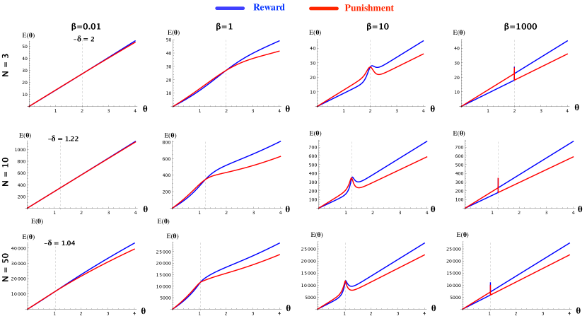
Figure 1: Compare the expected total cost of investment $E$ for reward and punishment, for varying $\theta$. Reward is less costly than punishment ($E_{r}<E_{p}$) for small $\theta$ and vice versa otherwise. The threshold of $\theta$ for this change was obtained analytically (see Theorem 1), which is exactly equal to $-\delta$. Other parameters: Donation Game with $b=2$, $c=1$.

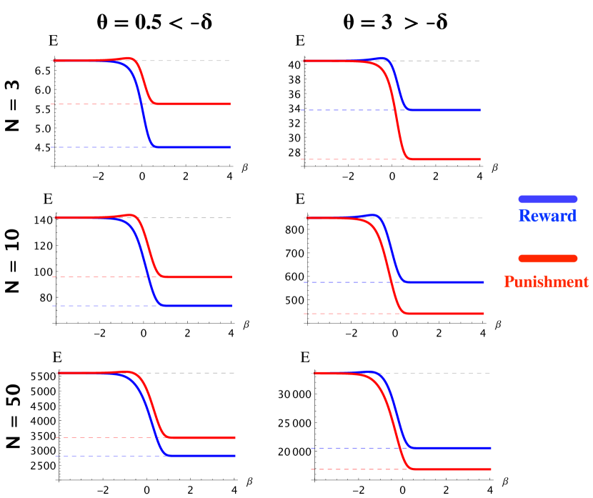
Figure 2: Total cost of incentive $E$ for reward and punishment, for different regimes of intensity of selection, $\beta$ (Log-10 scaled), from weak to strong selection limits. We show for different values of $N$. The dashed lines represent the corresponding theoretical limiting values obtained in Theorem 3.1 for weak and strong selection limits. We observe that numerical results are in close accordance with those obtained theoretically. Other parameters: Donation Game with $b=2$, $c=1$.

4.2 Numerical evaluation

We perform several numerical investigations to demonstrate the main theoretical results. To begin with, Figure 1 shows the expected total costs for reward and punishment (DG), for varying $\theta$. We observe that reward is less costly than punishment ($E_{r}<E_{p}$) for $\theta<-\delta$ and vice versa when $\theta>-\delta$. It is exactly as shown analytically in Theorem 3.1. This analytical result is confirmed here for different population size $N$ and intensity of selection $\beta$.

In Figure 2 we calculate the total costs of incentive for both reward and punishment for different regimes of intensity of selection. We observe that for both weak and strong limits of selection, the theoretical results obtained in Theorem 3.1 are confirmed, for different population sizes.

Now for Theorem 3.2 and Algorithm 3.3, we focus on reward for illustration. Figure 3 plots the cost function $E(\theta)$ (for institutional reward) in terms of $\theta$ for different values of $N$, $\beta$ and $\omega$ for illustrating the phase transition when varying $\beta$, in a DG. We can see that in all cases, these numerical observations are in close accordance with theoretical results. For example, with $N=3$ (see top row), we found $\beta^{\star}=f^{\star}/\delta=10.9291/1.9=5.752$. Similarly, in the second case, $\beta^{\star}=3.15/1.03673=3.039$. For $\beta<\beta^{\star}$, $E(\theta)$ are increasing functions of $\theta$. Thus, the optimal cost of incentive $\theta^{\star}=\theta_{0}$, for a given required minimum level of cooperation $\omega$. For example, with $N=3$, for $\beta=1$ to ensure at least 70% of cooperation ($\omega=0.7$), then $\theta^{\star}=\theta_{0}=2.32$. When $\beta\geq\beta^{\star}$ one needs to compare $E(\theta_{0})$ and $E(\theta_{2})$. For example, with $N=3$, $\beta=10$: for $\omega=0.25$ (black dashed line), then $E(\theta_{0})=23.602<25.6124=EC(\theta_{2})$, so $\theta^{\star}=\theta_{0}=1.845$; for $\omega=0.7$ (green dashed line), then $E(\theta_{0})=26.446>25.6124=EC(\theta_{2})$, so $\theta^{\star}=\theta_{2}=2.16$ (red solid line); for $\omega=0.999999$ (blue dashed line), since $\theta_{2}<\theta_{0}$, $\theta^{\star}=\theta_{0}=2.59078$.

Similarly, with a larger population size ($N=50$), we obtained $\beta^{\star}=3.039$. In general, similar observations are obtained as in case of a small population size $N=3$. Except that when $N$ is large, the values of $\theta_{0}$ for different non-extreme values of minimum required cooperation $\omega$ (say, $\omega\in(0.01,0.99)$) is very small (given the log scale of $\omega/(1-\omega)$ in the formula of $\omega_{0}$). This value is also smaller than $\theta_{0}$, with a cost $E(\theta_{0})>E(\theta_{2})$, making $\theta_{2}$ the optimal cost of incentive. Similar results are obtained for PGG (see Figure 2 in the Supporting Information). When $\omega$ is extremely high (i.e. $>1-10^{-k}$, for a large $k$) (we don’t look at extremely low value since we would like to ensure at least a sufficient level of cooperation), then we can also see other scenarios where the optimal cost is $\theta_{0}$ (see Figure 1 in the SI, bottom row). We thus can observe that for $\omega\in(0.01,0.99)$, for sufficiently large population size $N$ and large enough $\beta$ ($\beta>\beta^{\star}+\text{a bit more}$), then the optimal value of $\omega$ is always $\theta_{2}$. Otherwise, $\theta_{0}$ is the optimal cost.

Figure 3 in the SI plots the increase in the costs $\theta_{0}$, $\theta^{\star}$ and $E$ in order to increase the level of cooperation from $\epsilon$ to $1-\epsilon$.

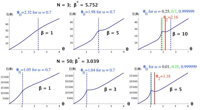
Figure 3: Using Algorithm 3.3 to find optimal $\theta$ that minimizes $E(\theta)$ (for institutional reward) while ensuring a minimum level of cooperation $\omega$. We use as examples a small population size ($N=3$, top row) and a larger one ($N=50$, bottom row), for Donation Game ($b=1.8$, $c=1$).

Figure 4: Using Algorithm 3.3 to find optimal $\theta$ that minimizes $E(\theta)$ while ensuring a minimum level of cooperation $\omega$, for PGG ($r=3$, $n=5$, $c=1$) with $N=50$. Similar observations to those with Donation Game, are obtained.

5 Discussion

Institutional incentives such as punishment and reward provide an effective tool for promoting the evolution of cooperation in social dilemmas. Both theoretical and experimental analysis has been provided (Gürerk et al., 2006; Sasaki et al., 2012; García and Traulsen, 2019; Baldassarri and Grossman, 2011; Dong et al., 2019; Bardhan, 2005; Wu et al., 2014). However, past research usually ignores the question of how institutions’ overall spending, i.e. the total cost of providing these incentives, can be minimized (while ensuring a desired level of cooperation). Answering this question allows one to estimate exactly how incentives should be provided, i.e. how much to reward a cooperator and how severely to punish a wrongdoer. Existing works that consider this question usually omit the stochastic effects in the population, namely, the intensity of selection.

Resorting to a stochastic evolutionary game approach for finite, well-mixed populations, we provide here theoretical results for the optimal cost of incentives that ensure a desired level of cooperation while minimizing the total budget, for a given intensity of selection, $\beta$. We show that this cost strongly depends on the value of $\beta$, due to the existence of a phase transition in the cost functions when $\beta$ varies. This behavior is missing in works that consider a deterministic evolutionary approach (Wang et al., 2019). The intensity of selection plays an important role in evolutionary processes. Its value differs depending on the payoff structure (i.e., scaling game payoff matrix by a factor is equivalent to dividing $\beta$ by that factor) and specific populations, which can be estimated in behavioral experiments (Traulsen et al., 2010; Rand et al., 2013; Zisis et al., 2015; Domingos et al., 2020). Thus, our analysis provides a way to calculate the optimal incentive cost for a given population and interaction game at hand.

As of theoretical importance, we characterize asymptotic behaviors of the total cost functions for both reward and punishment (namely, large population, weak selection and strong selection, limits) and compare these functions for the two types of incentive. We show that punishment is alway more costly for small (individual) incentive cost ($\theta$) but less so when this cost is above a certain threshold. This result provides insights into the choice of which type of incentives to use. We provide an exact formula for this threshold. Moreover, we provide numerical validation of the theoretical results.

In the context of institutional incentives modelling, a crucial issue is the question of how to maintain the budget of incentives providing. The problem of who pays or contributes to the budget is a social dilemma itself, and how to escape this dilemma is critical research question. In this work we focus on the question of how to optimize the budget used for provided incentives. For future research, we plan to generalise the results of this paper to more complex scenarios such as other social dilemmas, mixed incentives, network effects, and any mutation.

6 Acknowledgements

T.A.H. acknowledges support from Leverhulme Research Fellowship (RF-2020-603/9) and Future of Life Institute (grant RFP2-154).

See pages - of SI-arxiv.pdf

References

- Antonioni and Cardillo [2017] Alberto Antonioni and Alessio Cardillo. Coevolution of synchronization and cooperation in costly networked interactions. Physical review letters, 118(23):238301, 2017.
- Baldassarri and Grossman [2011] Delia Baldassarri and Guy Grossman. Centralized sanctioning and legitimate authority promote cooperation in humans. Proceedings of the National Academy of Sciences, 108(27):11023–11027, 2011.
- Bardhan [2005] Pranab Bardhan. Institutions matter, but which ones? Economics of transition, 13(3):499–532, 2005.
- Bowles [2009] Samuel Bowles. Microeconomics: behavior, institutions, and evolution. Princeton University Press, 2009.
- Bowles and Gintis [2002] Samuel Bowles and Herbert Gintis. Social capital and community governance. The economic journal, 112(483):F419–F436, 2002.
- Boyd et al. [2003] Robert Boyd, Herbert Gintis, Samuel Bowles, and Peter J. Richerson. The evolution of altruistic punishment. Proceedings of the National Academy of Sciences, 100(6):3531–3535, March 2003. doi: 10.1073/pnas.0630443100. URL http://dx.doi.org/10.1073/pnas.0630443100.
- Boyd et al. [2010] Robert Boyd, Herbert Gintis, and Samuel Bowles. Coordinated punishment of defectors sustains cooperation and can proliferate when rare. Science, 328(5978):617–620, 2010.
- Chen et al. [2015] Xiaojie Chen, Tatsuya Sasaki, Åke Brännström, and Ulf Dieckmann. First carrot, then stick: how the adaptive hybridization of incentives promotes cooperation. Journal of The Royal Society Interface, 12(102):20140935, 2015.
- Cimpeanu et al. [2019] Theodor Cimpeanu, The Anh Han, and Francisco C Santos. Exogenous rewards for promoting cooperation in scale-free networks. In The 2018 Conference on Artificial Life: A Hybrid of the European Conference on Artificial Life (ECAL) and the International Conference on the Synthesis and Simulation of Living Systems (ALIFE), pages 316–323. MIT Press, 2019.
- Domingos et al. [2020] Elias Fernández Domingos, Jelena Grujić, Juan C Burguillo, Georg Kirchsteiger, Francisco C Santos, and Tom Lenaerts. Timing uncertainty in collective risk dilemmas encourages group reciprocation and polarization. Iscience, 23(12):101752, 2020.
- Dong et al. [2019] Yali Dong, Tatsuya Sasaki, and Boyu Zhang. The competitive advantage of institutional reward. Proceedings of the Royal Society B: Biological Sciences, 286(1899):20190001, 2019.
- Fehr and Gachter [2000] Ernst Fehr and Simon Gachter. Cooperation and punishment in public goods experiments. American Economic Review, 90(4):980–994, 2000.
- Fudenberg and Imhof [2005] D. Fudenberg and L. A. Imhof. Imitation processes with small mutations. Journal of Economic Theory, 131:251–262, 2005.
- García and Traulsen [2019] Julián García and Arne Traulsen. Evolution of coordinated punishment to enforce cooperation from an unbiased strategy space. Journal of the Royal Society Interface, 16(156):20190127, 2019.
- Góis et al. [2019] António R Góis, Fernando P Santos, Jorge M Pacheco, and Francisco C Santos. Reward and punishment in climate change dilemmas. Scientific reports, 9(1):1–9, 2019.
- Gürerk et al. [2006] Özgür Gürerk, Bernd Irlenbusch, and Bettina Rockenbach. The competitive advantage of sanctioning institutions. Science, 312(5770):108–111, 2006.
- Hamilton [1964] W.D. Hamilton. The genetical evolution of social behaviour. i. Journal of Theoretical Biology, 7(1):1 – 16, 1964. ISSN 0022-5193. doi: 10.1016/0022-5193(64)90038-4. URL http://www.sciencedirect.com/science/article/pii/0022519364900384.
- Han et al. [2012] T. A. Han, L. M. Pereira, and F. C. Santos. Corpus-based intention recognition in cooperation dilemmas. Artificial Life, 18(4):365–383, 2012.
- Han et al. [2013] T. A. Han, L. M. Pereira, F. C. Santos, and T. Lenaerts. Good agreements make good friends. Scientific reports, 3(2695), 2013.
- Han [2013] The Anh Han. Intention Recognition, Commitments and Their Roles in the Evolution of Cooperation: From Artificial Intelligence Techniques to Evolutionary Game Theory Models, volume 9. Springer SAPERE series, 2013. ISBN 978-3-642-37511-8.
- Han and Tran-Thanh [2018] The Anh Han and Long Tran-Thanh. Cost-effective external interference for promoting the evolution of cooperation. Scientific reports, 8(1):1–9, 2018.
- Han et al. [2016] The Anh Han, Luís Moniz Pereira, and Tom Lenaerts. Evolution of commitment and level of participation in public goods games. Autonomous Agents and Multi-Agent Systems, pages 1–23, 2016. ISSN 1573-7454. doi: 10.1007/s10458-016-9338-4. URL http://dx.doi.org/10.1007/s10458-016-9338-4.
- Han et al. [2018] The Anh Han, Simon Lynch, Long Tran-Thanh, and Francisco C. Santos. Fostering cooperation in structured populations through local and global interference strategies. In IJCAI-ECAI’2018, pages 289–295, 2018.
- Han et al. [2021] The Anh Han, Luis Moniz Pereira, Tom Lenaerts, and Francisco C. Santos. Mediating Artificial Intelligence Developments through Negative and Positive Incentives. PLOS ONE, 16(1):e0244592, 2021. doi: 10.1371/journal.pone.0244592.
- Hauert et al. [2007a] C. Hauert, A. Traulsen, H. Brandt, M. A. Nowak, and K. Sigmund. Via freedom to coercion: The emergence of costly punishment. Science, 316:1905–1907, 2007a.
- Hauert et al. [2007b] Christoph Hauert, Arne Traulsen, Hannelore Brandt, Martin A Nowak, and Karl Sigmund. Via freedom to coercion: the emergence of costly punishment. science, 316(5833):1905–1907, 2007b.
- Herrmann et al. [2008] Benedikt Herrmann, Christian Thöni, and Simon Gächter. Antisocial Punishment Across Societies. Science, 319(5868):1362–1367, March 2008.
- Hofbauer and Sigmund [1998] J. Hofbauer and K. Sigmund. Evolutionary Games and Population Dynamics. Cambridge University Press, 1998.
- Huang and McColl [1997] Y Huang and W F McColl. Analytical inversion of general tridiagonal matrices. Journal of Physics A: Mathematical and General, 30(22):7919–7933, nov 1997. doi: 10.1088/0305-4470/30/22/026. URL https://doi.org/10.1088%2F0305-4470%2F30%2F22%2F026.
- Imhof et al. [2005] L. A. Imhof, D. Fudenberg, and Martin A. Nowak. Evolutionary cycles of cooperation and defection. Proc. Natl. Acad. Sci. U.S.A., 102:10797–10800, 2005.
- Karlin and Taylor [1975] S. Karlin and H. E. Taylor. A First Course in Stochastic Processes. Academic Press, New York, 1975.
- Kemeny and Snell [1976] J. Kemeny and J. Snell. Finite Markov Chains. Undergraduate Texts in Mathematics. Springer, 1976.
- Krellner and Han [2020] Marcus Krellner and The Anh Han. Putting oneself in everybody’s shoes-pleasing enables indirect reciprocity under private assessments. In Artificial Life Conference Proceedings, pages 402–410. MIT Press, 2020.
- Martinez-Vaquero et al. [2017] Luis A Martinez-Vaquero, The Anh Han, Luis Moniz Pereira, and Tom Lenaerts. When agreement-accepting free-riders are a necessary evil for the evolution of cooperation. Scientific reports, 7(1):1–9, 2017.
- Nesse [2001] R. M. Nesse. Evolution and the capacity for commitment. Foundation series on trust. Russell Sage, 2001. ISBN 9780871546227.
- Nowak [2006a] M. A. Nowak. Evolutionary Dynamics: Exploring the Equations of Life. Harvard University Press, Cambridge, MA, 2006a.
- Nowak and Sigmund [2005] M. A. Nowak and K. Sigmund. Evolution of indirect reciprocity. Nature, 437(1291-1298), 2005.
- Nowak et al. [2004] M. A. Nowak, A. Sasaki, C. Taylor, and D. Fudenberg. Emergence of cooperation and evolutionary stability in finite populations. Nature, 428:646–650, 2004.
- Nowak [2006b] Martin A. Nowak. Five rules for the evolution of cooperation. Science, 314(5805):1560, 2006b.
- Ohtsuki and Iwasa [2006] Hisashi Ohtsuki and Yoh Iwasa. The leading eight: Social norms that can maintain cooperation by indirect reciprocity. Journal of Theoretical Biology, 239(4):435 – 444, 2006. ISSN 0022-5193. doi: DOI:10.1016/j.jtbi.2005.08.008. URL http://www.sciencedirect.com/science/article/B6WMD-4H4T62M-1/2/fda30e013d634e1c0b30a4559c2342bb.
- Okada [2020] Isamu Okada. A review of theoretical studies on indirect reciprocity. Games, 11(3):27, 2020.
- Ostrom [1990] Elinor Ostrom. Governing the commons: The evolution of institutions for collective action. Cambridge university press, 1990.
- Peña et al. [2016] Jorge Peña, Bin Wu, Jordi Arranz, and Arne Traulsen. Evolutionary games of multiplayer cooperation on graphs. PLoS computational biology, 12(8):e1005059, 2016.
- Perc et al. [2013] Matjaž Perc, Jesús Gómez-Gardeñes, Attila Szolnoki, Luis M Floría, and Yamir Moreno. Evolutionary dynamics of group interactions on structured populations: a review. Journal of The Royal Society Interface, 10(80):20120997, 2013.
- Perc et al. [2017] Matjaž Perc, Jillian J Jordan, David G Rand, Zhen Wang, Stefano Boccaletti, and Attila Szolnoki. Statistical physics of human cooperation. Phys Rep, 687:1–51, 2017.
- Powers et al. [2018] Simon T Powers, Anikó Ekárt, and Peter R Lewis. Modelling enduring institutions: The complementarity of evolutionary and agent-based approaches. Cognitive Systems Research, 52:67–81, 2018.
- Rand et al. [2013] David G. Rand, Corina E. Tarnita, Hisashi Ohtsuki, and Martin A. Nowak. Evolution of fairness in the one-shot anonymous ultimatum game. Proc. Natl. Acad. Sci. USA, 110:2581–2586, 2013.
- Santos et al. [2006] F. C. Santos, J. M. Pacheco, and T. Lenaerts. Evolutionary dynamics of social dilemmas in structured heterogeneous populations. Proceedings of the National Academy of Sciences of the United States of America, 103:3490–3494, 2006. ISSN 0027-8424.
- Sasaki et al. [2012] Tatsuya Sasaki, Åke Brännström, Ulf Dieckmann, and Karl Sigmund. The take-it-or-leave-it option allows small penalties to overcome social dilemmas. Proceedings of the National Academy of Sciences, 109(4):1165–1169, 2012.
- Sasaki et al. [2015] Tatsuya Sasaki, Isamu Okada, Satoshi Uchida, and Xiaojie Chen. Commitment to cooperation and peer punishment: Its evolution. Games, 6(4):574–587, 2015.
- Scotchmer [2004] Suzanne Scotchmer. Innovation and incentives. MIT press, 2004.
- Sigmund et al. [2001] K Sigmund, C Hauert, and M Nowak. Reward and punishment. P Natl Acad Sci USA, 98(19):10757–10762, 2001.
- Sigmund et al. [2010] K. Sigmund, H. De Silva, A. Traulsen, and C. Hauert. Social learning promotes institutions for governing the commons. Nature, 466:7308, 2010.
- Sigmund [2010] Karl Sigmund. The Calculus of Selfishness. Princeton University Press, 2010.
- Traulsen and Nowak [2006] A. Traulsen and M. A. Nowak. Evolution of cooperation by multilevel selection. Proceedings of the National Academy of Sciences of the United States of America, 103(29):10952, 2006.
- Traulsen et al. [2006] A. Traulsen, M. A. Nowak, and J. M. Pacheco. Stochastic dynamics of invasion and fixation. Phys. Rev. E, 74:11909, 2006.
- Traulsen et al. [2010] Arne Traulsen, Dirk Semmann, Ralf D Sommerfeld, Hans-Jürgen Krambeck, and Manfred Milinski. Human strategy updating in evolutionary games. Proceedings of the National Academy of Sciences, 107(7):2962–2966, 2010.
- Vasconcelos et al. [2013] Vitor V Vasconcelos, Francisco C Santos, and Jorge M Pacheco. A bottom-up institutional approach to cooperative governance of risky commons. Nature Climate Change, 3(9):797, 2013.
- Wang et al. [2019] Shengxian Wang, Xiaojie Chen, and Attila Szolnoki. Exploring optimal institutional incentives for public cooperation. Communications in Nonlinear Science and Numerical Simulation, 79:104914, 2019.
- West et al. [2007] S.A. West, A.A. Griffin, and A. Gardner. Evolutionary explanations for cooperation. Current Biology, 17:R661–R672, 2007.
- Wu et al. [2014] Jia-Jia Wu, Cong Li, Bo-Yu Zhang, Ross Cressman, and Yi Tao. The role of institutional incentives and the exemplar in promoting cooperation. Scientific reports, 4:6421, 2014.
- Young [1991] R. M. Young. 75.9 euler’s constant. The Mathematical Gazette, 75(472):187–190, 1991.
- Zisis et al. [2015] Ioannis Zisis, Sibilla Di Guida, The Anh Han, Georg Kirchsteiger, and Tom Lenaerts. Generosity motivated by acceptance - evolutionary analysis of an anticipation games. Scientific reports, 5(18076), 2015.