Thermal coherence of the Heisenberg model with Dzyaloshinsky-Moriya interactions in an inhomogenous external field

Abstract

The quantum coherence of the two-site XYZ model with Dzyaloshinsky-Moriya (DM) interactions in an external inhomogenous magnetic field is studied. The DM interaction, the magnetic field and the measurement basis can be along different directions, and we examine the quantum coherence at finite temperature. With respect to the spin-spin interaction parameter, we find that the quantum coherence decreases when the direction of measurement basis is the same as that of the spin-spin interaction. When the spin-lattice interaction is varied, the coherence always increases irrespective of the relation between its direction and the measurement basis. Similar analysis of quantum coherence based on the variation of the external inhomogenous magnetic field is also carried out, where we find that the coherence decreases when the direction of the measurement basis is the same as that of the external field.

CAPS Number(s): 05.20.G, 05.70.Ce, 02.30.GP
Keywords: anisotropic spin model, DM interaction, quantum coherence.

I Introduction

Quantum coherence has been a central concept in the theory of quantum mechanics since its earliest days. In the context of quantum optics, coherence was investigated using phase space distributions and higher order correlation functions Glauber (1963); Sudarshan (1963). It was only recently that a rigorous quantum information theoretic framework for measuring coherence was developed, in the seminal paper by Baumgratz, Cramer and Plenio Baumgratz et al. (2014). The work introduced a set of axioms which are necessary for a mathematical function to be a proper quantifier of quantum coherence. In Ref. Baumgratz et al. (2014), two measures of quantum coherence were introduced based on these axioms, namely the relative entropy measure of coherence and the $\ell_{1}$-norm based quantum coherence. The fundamental properties of quantum coherence have been investigated Yao et al. (2015); Yadin et al. (2015); Ma et al. (2016); Yadin and Vedral (2016); Bromley et al. (2015); Du et al. (2015); Pires et al. (2015); Cheng and Hall (2015); Streltsov et al. (2015) and also their applications in different quantum phenomena Shi et al. (2017); Hillery (2016); Zhang et al. (2019); Ma et al. (2019); Narasimhachar and Gour (2015) have been studied. These investigations also gave rise to the resource theory framework of quantum coherence Winter and Yang (2016); Brandão and Gour (2015); Chitambar and Hsieh (2015); Chitambar and Gour (2016); del Rio et al. (2015); Streltsov et al. (2015); Chitambar and Gour (2019); Radhakrishnan et al. (2016).

Quantum coherence has been investigated with regards to search algorithms Shi et al. (2017); Hillery (2016), quantum thermodynamics Narasimhachar and Gour (2015); Lostaglio et al. (2015) and quantum metrology Ma et al. (2019). Previous studies have established applications of quantum coherence in quantum information processing tasks like quantum dense coding and teleportation Pan et al. (2017). Another important application of quantum coherence is in the characterization of quantum states. Multipartite systems have a large number of degrees of freedom, and it is of interest to understand what type of coherences a given state possesses. Such a scheme was introduced in Ref. Radhakrishnan et al. (2016), where coherence could be subdivided into its constituent parts. Quantum simulation Georgescu et al. (2014) is a prime example of where this can be applied, since the naturally arising states of a condensed matter system can show strikingly different properties depending upon the physical parameters driving phase transitions in the system. In the field of condensed matter physics, the measurement and properties of quantum coherence has been studied in various models Opanchuk et al. (2016); Zheng et al. (2016); Ishida et al. (2013); Karpat et al. (2014). Heisenberg spin models Lieb et al. (1961); Niemeijer (1967, 1968); Barouch et al. (1970); Barouch and McCoy (1971); Giamarchi (2004) are one of the important class of models in which coherence has been investigated Malvezzi et al. (2016); Li and Lin (2016); Cheng et al. (2016); Çakmak et al. (2015), where one of the main themes has been the investigation of quantum phase transitionLi and Lin (2016); Cheng et al. (2016); Çakmak et al. (2015); Radhakrishnan et al. (2017a). In the Heisenberg XYZ model, the spins have a direct interaction between nearby sites. In addition, they can also have a spin-lattice interaction generally referred to as the Dzyaloshinsky-Moriya (DM) interaction Dzyaloshinsky (1958); Moriya (1960). Spins are usually aligned parallel or anti-parallel to each other depending on whether it is in the ferromagnetic phase or antiferromagnetic phase. Due to the spin-lattice interaction the spins are tilted at an angle to the parallel, a feature known as spin-canting. This spin-canting usually leads to weak ferromagnetic behavior even in an antiferromagnetic system. In addition to these inherent properties, it is also possible to apply an external magnetic field to the spin system to control and modify its quantum properties.

A minimal example of the DM model is the two-site model which has been studied to understand the overall dependence of quantities such as entanglement Wang (2001); Zhou et al. (2003); Li and Cao (2008); Kheirandish et al. (2008); Li and Cao (2009); Gurkan and Pashaev (2010), quantum discord Guo et al. (2011); Zidan (2014); Yi-Xin and Zhi (2010), and coherence Radhakrishnan et al. (2017b) as a function of the various parameters of the system. In Ref. Radhakrishnan et al. (2017b), a detailed investigation of quantum coherence in two-spin models were carried out. In this paper, we extend the investigations carried out in Ref. Radhakrishnan et al. (2017b) and investigate two-spin models with DM interactions in the presence of an external field. A detailed analysis of the dependence of the quantum coherence on various parameters such as the spin-spin interaction, the spin-orbit interaction, DM interaction, and external magnetic field is carried out. As quantum coherence is a basis dependent quantity, in our work we choose different orientations of the DM interaction parameter and the external fields keeping the measurement direction in the $\sigma_{z}$ basis for all cases. This will help us to understand the basis-dependent nature of coherence with respect to the internal parameters such as spin-spin interaction, as well as the DM interaction parameter. Finally, the relation between quantum coherence and the external driving forces such as the homogeneous component and the inhomogenous component of the magnetic field will be explored.

The article is structured as follows: In Sec. III we discuss the quantum coherence dependence in the two-spin XYZ model with DM interactions and external field in the same direction. The features of quantum coherence where the two-site XYZ model with the DM interaction and external field in different directions is discussed in Sec. IV. Sec. V gives the simultaneous variation of the quantum coherence with spin-spin interaction and any one of the other parameters such as DM interaction, homogeneous component, or the inhomogenous component of the external field. Finally, we present our conclusions in Sec. VI.

II The Heisenberg model with DM interaction and the coherence measure

The Heisenberg spin model consists of a collection of interacting spins arranged periodically on a lattice. The Hamiltonian of the Heisenberg spin chain is written as

$$H=\sum_{n}J_{x}\sigma_{n}^{x}\sigma_{n+1}^{x}+J_{y}\sigma_{n}^{y}\sigma_{n+1}^{y}+J_{z}\sigma_{n}^{z}\sigma_{n+1}^{z},$$ (1)

where $\sigma_{n}^{x,y,z}$ are the Pauli spin matrices at the site $n$ and $J_{x,y,z}$ are the spin-spin interaction terms in the $x$,$y$ and $z$ directions. For $J_{x}\neq J_{y}\neq J_{z}$, the spin model is referred to as XYZ model. The model is antiferromagnetic when $J_{i}>0$ $(i=x,y,x)$ and ferromagnetic for $J_{i}<0$. Along with the spin-spin interaction we may also have a spin-lattice interaction which are known as the Dzyaloshinsky-Moriya (DM) interaction. The Hamiltonian of the XYZ spin chain with the DM interaction is

$$H=\sum_{n}J_{x}\sigma_{n}^{x}\sigma_{n+1}^{x}+J_{y}\sigma_{n}^{y}\sigma_{n+1}^{y}+J_{z}\sigma_{n}^{z}\sigma_{n+1}^{z}+\vec{D}.(\vec{\sigma}_{n}\times\vec{\sigma}_{n+1})$$ (2)

The antisymmetric spin-lattice interaction is accounted for by the DM interaction coefficient $\vec{D}$.

In our work we further consider an inhomogenous external magnetic field. The Hamiltonian of a two-spin system with DM interaction in an external inhomogenous field is

$$H=J_{x}\sigma_{1}^{x}\sigma_{2}^{x}+J_{y}\sigma_{1}^{y}\sigma_{2}^{y}+J_{z}\sigma_{1}^{z}\sigma_{2}^{z}+\vec{D}\cdot(\vec{\sigma}_{1}\times\vec{\sigma}_{2})+(\vec{B}+\vec{b})\cdot\vec{\sigma}_{1}^{j}+(\vec{B}-\vec{b})\cdot\vec{\sigma}_{2}^{j}.$$ (3)

This field can be written as two fields of the form $\vec{B}+\vec{b}$ acting on the first qubit and the field $\vec{B}-\vec{b}$ acting on the second qubit, where $B$ is the homogeneous and $b$ is the inhomogenous component of the external magnetic field.

From the Hamiltonian of this model, the quantum properties can be studied by examining its eigenstates. In our work, we investigate the quantum coherence of the system at finite (non-zero) temperature. Quantum coherence is measured as the distance between the density matrix $\rho$ and the decohered density matrix $\rho_{d}$. The decohered density matrix is defined according to the matrix elements

$$\langle\sigma_{1}\sigma_{2}|\rho_{d}|\sigma_{1}^{\prime}\sigma_{2}^{\prime}\rangle=\langle\sigma_{1}\sigma_{2}|\rho|\sigma_{1}^{\prime}\sigma_{2}^{\prime}\rangle\delta_{\sigma_{1},\sigma_{1}^{\prime}}\delta_{\sigma_{2},\sigma_{2}^{\prime}}.$$ (4)

In Ref. (Baumgratz et al., 2014), two different measures of coherence namely the relative entropy measure belonging to the entropic class and the $\ell_{1}$-norm of coherence which is a geometric measure were introduced. Another measure based on the quantum version of the Jensen-Shannon divergence Lin (1991); Lamberti et al. (2008); Briët and Harremoës (2009) was introduced in Ref. Radhakrishnan et al. (2016)

$$\mathcal{D}(\rho,\sigma)\equiv\sqrt{J(\rho,\sigma)}=\sqrt{S\left(\frac{\rho+\sigma}{2}\right)-\frac{S(\rho)}{2}-\frac{S(\sigma)}{2}}.$$ (5)

Here $\rho,\sigma$ are arbitrary density matrices and $S=-{\rm Tr}\rho\log\rho$ is the von Neumann entropy. This measure has the advantage that it has both geometric and entropic properties and is also a metric satisfying triangle inequality. The coherence is then defined in our case as

$${\cal C}(\rho)=\mathcal{D}(\rho,\rho_{d}).$$ (6)

The coherence of the two-spin XYZ model in Eq. (3) at finite temperature is discussed in the rest of the paper. Since quantum coherence is a basis-dependent quantity we examine the spin model in two different cases namely: ($i$) when the control parameters and measurement basis are in the same direction; ($ii$) when the control parameters like DM interaction and the external field are orthogonal to the measurement basis.

III DM interaction and the external magnetic field along the same direction

A $\vec{D}\propto\vec{x},\vec{B}\propto\vec{x}$ case

For the case where both the DM interaction and the external magnetic field are in the $x$ direction, the Hamiltonian reads

$$H=J_{x}\sigma_{1}^{x}\sigma_{2}^{x}+J_{y}\sigma_{1}^{y}\sigma_{2}^{y}+J_{z}\sigma_{1}^{z}\sigma_{2}^{z}+D_{x}(\sigma_{1}^{y}\sigma_{2}^{z}-\sigma_{1}^{z}\sigma_{2}^{y})+(B_{x}+b_{x})\sigma_{1}^{x}+(B_{x}-b_{x})\sigma_{2}^{x},$$ (7)

where $D_{x}$ is the DM interaction in the $x$-direction, and $B_{x}$ is the average magnetic field and $b_{x}$ is the inhomogneous magnetic field in the $x$-direction. The matrix representation of the Hamiltonian in the $\sigma_{z}$-basis is

$$H=\left(\begin{array}[]{cccc}J_{z}&G_{2}&G_{3}&J_{-}\\ G_{4}&-J_{z}&J_{+}&G_{1}\\ G_{1}&J_{+}&-J_{z}&G_{4}\\ J_{-}&G_{3}&G_{2}&J_{z}\\ \end{array}\right),$$ (8)

where $G_{1,2}=iD_{x}+B_{x}\pm b_{x}$, $G_{3,4}=G_{1,2}^{*}$ and $J_{\pm}=J_{x}\pm J_{y}$. The eigenvalues of the Hamiltonian are

$$E_{1,2}=J_{x}\pm\omega_{1},\qquad E_{3,4}=-J_{x}\pm\omega_{2},$$ (9)

and their corresponding eigenvectors are

$$|\psi_{1,2}\rangle = \frac{1}{\sqrt{2}}(\sin\varphi_{1,2}|00\rangle+\cos\varphi_{1,2}|01\rangle+\cos\varphi_{1,2}|10\rangle+\sin\varphi_{1,2}|11\rangle)$$ (10)

$$|\psi_{3,4}\rangle = \frac{1}{\sqrt{2}}(\sin\varphi_{3,4}|00\rangle+\chi\cos\varphi_{3,4}|01\rangle-\chi\cos\varphi_{3,4}|10\rangle-\sin\varphi_{3,4}|11\rangle)$$ (11)

where the various factors used are

$$\chi = \frac{-iD_{x}-b_{x}}{\sqrt{b_{x}^{2}+D_{x}^{2}}},\quad\omega_{1}=\sqrt{4B_{x}^{2}+(J_{y}-J_{z})^{2}},\quad\omega_{2}=\sqrt{4b_{x}^{2}+4D_{x}^{2}+(J_{y}+J_{z})^{2}}$$

$$\varphi_{1,2} = \arctan\left(\frac{2B_{x}}{J_{y}-J_{z}\pm\omega_{1}}\right),\quad\varphi_{3,4}=\arctan\left(\frac{2\sqrt{b_{x}^{2}+D_{x}^{2}}}{-J_{y}-J_{z}\pm\omega_{2}}\right).$$ (12)

The state of the two-spin spin system at thermal equilibrium is given by the thermal density matrix $\rho(T)=\exp(-\beta H)/Z$ where $Z={\hbox{Tr}}[\exp(-\beta H)]$ is the partition function of the system and $\beta=1/k_{B}T$, and $k_{B}$ and $T$ are the Boltzmann constant and temperature respectively. For the sake of convenience we assume $k_{B}=1$ throughout our discussion. The matrix form of the thermal density matrix in the $\sigma_{z}$-basis is

$$\rho(T)=\left(\begin{array}[]{cccc}u_{1}&q_{1}^{*}&q_{2}^{*}&u_{2}\\ q_{1}&v_{1}&v_{2}&q_{2}\\ q_{2}&v_{2}&v_{1}&q_{1}\\ u_{2}&q_{2}^{*}&q_{1}^{*}&u_{1}\\ \end{array}\right).$$ (13)

The elements of the thermal density matrix (13) are

$$u_{1,2} = \frac{1}{2Z}\left[e^{-\frac{J_{x}+\omega_{1}}{T}}\sin^{2}\varphi_{1}+e^{-\frac{J_{x}-\omega_{1}}{T}}\sin^{2}\varphi_{2}\pm e^{\frac{J_{x}-\omega_{2}}{T}}\sin^{2}\varphi_{3}\pm e^{\frac{J_{x}+\omega_{2}}{T}}\sin^{2}\varphi_{4}\right],$$ (14)

$$v_{1,2} = \frac{1}{2Z}\left[e^{-\frac{J_{x}+\omega_{1}}{T}}\cos^{2}\varphi_{1}+e^{-\frac{J_{x}-\omega_{1}}{T}}\cos^{2}\varphi_{2}\pm e^{\frac{J_{x}-\omega_{2}}{T}}\cos^{2}\varphi_{3}\pm e^{\frac{J_{x}+\omega_{2}}{T}}\cos^{2}\varphi_{4}\right],$$ (15)

$$q_{1,2} = \frac{1}{2Z}\Big{[}e^{-\frac{J_{x}+\omega_{1}}{T}}\sin\varphi_{1}\cos\varphi_{1}+e^{-\frac{J_{x}-\omega_{1}}{T}}\sin\varphi_{2}\cos\varphi_{2}\pm e^{\frac{J_{x}-\omega_{2}}{T}}\chi\sin\varphi_{3}\cos\varphi_{3}$$ (16)

$$\pm e^{\frac{J_{x}+\omega_{2}}{T}}\chi\sin\varphi_{4}\cos\varphi_{4}\Big{]}.$$

where the partition function is

$$Z=2\left[e^{-\frac{J_{x}}{T}}\cosh\left(\frac{\omega_{1}}{T}\right)+e^{\frac{J_{x}}{T}}\cosh\left(\frac{\omega_{2}}{T}\right)\right].$$ (17)

From the density matrix $\rho(T)$, we can write down the decohered density matrix $\rho_{d}$ using which we can measure coherence introduced through Eq. (6).

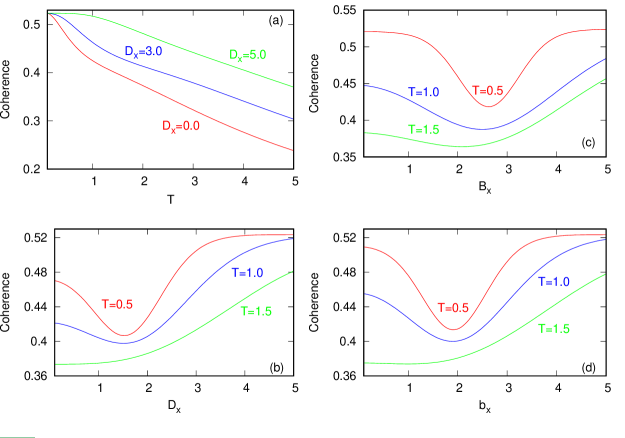
Figure 1: Quantum coherence measurement in $\sigma_{z}$ basis in the XYZ model with DM interactions in the $x$-direction and the external magnetic field in the $x$-direction. (a) Quantum coherence versus temperature $T$ for different $D_{x}$, for $B_{x}=3.0$, $b_{x}=1.5$, $J_{x}=0.8$, $J_{y}=0.5$ and $J_{z}=0.2$. (b) Quantum coherence versus $D_{x}$ for different temperatures $T$, for $B_{x}=3.0$, $b_{x}=1.5$, $J_{x}=0.8$, $J_{y}=0.5$ and $J_{z}=0.2$. (c) Quantum coherence versus $B_{x}$ for different temperatures $T$, for $D_{x}=1.0$, $b_{x}=1.5$, $J_{x}=0.8$, $J_{y}=0.5$ and $J_{z}=0.2$. (d) Quantum coherence versus $b_{x}$ for different temperatures $T$, for $D_{x}=1.0$, $B_{x}=3.0$, $J_{x}=0.8$, $J_{y}=0.5$ and $J_{z}=0.2$.

The behavior of quantum coherence is shown in Fig. 1. Since quantum coherence is a basis dependent quantity, the choice of measurement basis plays an important role. In the Hamiltonian of Eq. (7), the DM interaction and the field are in the $x$-direction, and the measurement is carried out in the $z$-direction. This behavior of coherence is very similar to the entanglement results reported in Ref. Li and Cao (2008). In Fig. 1(a) the variation of coherence with temperature is shown and we find that coherence decreases with temperature. This can be explained by the thermal fluctuations inducing decoherence in the quantum system, thereby decreasing coherence. The rate of decrease of coherence is lower for higher values of the DM interaction parameter. This is because the DM interaction creates an extra spin-lattice coupling apart from the existing spin-spin coupling. This additional spin lattice coupling gives rise to additional coherence in the quantum system. The variation of quantum coherence with the DM interaction parameter is shown in Fig. 1(b) for different values of temperature. We find that for lower values of temperature ($T=0.5,T=1.0$), the coherence decreases initially, reaches a minimum value and then increases to reach a saturation value. Initially at $D_{x}=0$, the spin-spin interaction is dominant and when it is increased the spin-lattice interaction is slowly introduced. The initial decrease in the spin-lattice interaction might be due to the competing effects of the spin-spin and spin-lattice interaction. The increase later on can be attributed to the co-operation between the spin-spin and spin-lattice interaction. At higher values of temperature ($T=1.5$), the coherence increases gradually to a saturation value.

The variation of the quantum coherence is investigated as a function of the external magnetic field in Fig. 1(c) and 1(d). We now examine the role played by the external inhomogenous field. In Fig. 1(c) we show the variation of quantum coherence with the field $B_{x}$ and we find that for the lower values of temperature, the coherence initially decreases and reaches a minimum value and then increases to attain a saturation value. For the higher values of temperature, the coherence increases with the homogeneous field $B_{x}$. The overall behavior of the quantum coherence with the inhomogenous field $b_{x}$ resembles the variation of coherence with the field $B_{x}$ as we can see from a comparison between Figs. 1(c) and 1(d). On comparison with the earlier works Ref. Li and Cao (2008) we find that quantum coherence exhibits behavior very similar to entanglement. From concurrence measurements one can see that entanglement also increases with the DM interaction. The main reason is that the entire coherence comes from the two-spin correlation in a manner similar to entanglement.

B $\vec{D}\propto\vec{z},\vec{B}\propto\vec{z}$ case

For the case where the DM interaction and the external magnetic field along the $z$-direction, the Hamiltonian reads

$$H=J_{x}\sigma_{1}^{x}\sigma_{2}^{x}+J_{y}\sigma_{1}^{y}\sigma_{2}^{y}+J_{z}\sigma_{1}^{z}\sigma_{2}^{z}+D_{z}(\sigma_{1}^{x}\sigma_{2}^{y}-\sigma_{1}^{y}\sigma_{2}^{x})+(B_{z}+b_{z})\sigma_{1}^{z}+(B_{z}-b_{z})\sigma_{2}^{z}.$$ (18)

Here, $B_{z}$ is the average external magnetic field in the $z$ direction and $b_{z}$ is the degree of inhomogenity of the field in the $z$-direction. In the standard measurement basis ($\sigma_{z}$ basis) the Hamiltonian can be written in matrix form as

$$H=\left(\begin{array}[]{cccc}2B_{z}+J_{z}&0&0&J_{x}-J_{y}\\ 0&2b_{z}-J_{z}&2iD_{z}+J_{x}+J_{y}&0\\ 0&-2iD_{z}+J_{x}+J_{y}&-2b_{z}-J_{z}&0\\ J_{x}-J_{y}&0&0&-2B_{z}+J_{z}\\ \end{array}\right).$$ (19)

The eigenvalues and eigenvectors corresponding to the Hamiltonian are

$$E_{1,2} = J_{z}+\omega_{1}\qquad|\psi_{1,2}\rangle=\sin\theta_{1,2}|00\rangle+\cos\theta_{1,2}|11\rangle,$$ (20)

$$E_{3,4} = -J_{z}+\omega_{2}\qquad|\psi_{3,4}\rangle=\sin\theta_{3,4}|01\rangle+\chi\cos\theta_{3,4}|10\rangle,$$ (21)

where the factors $\omega_{1}$ and $\omega_{2}$ are

$$\omega_{1}=\sqrt{4B_{z}^{2}+(J_{x}-J_{y})^{2}},\qquad\omega_{2}=\sqrt{4b_{z}^{2}+4D_{z}^{2}+(J_{x}+J_{y})^{2}}.$$ (22)

In the expression for the eigenvectors the parameters used are

$$\theta_{1,2}=\arctan\left(\frac{J_{x}-J_{y}}{\pm\omega_{1}-2B_{z}}\right),\qquad\theta_{3,4}=\arctan\left(\frac{\sqrt{(J_{x}+J_{y})^{2}+D_{z}^{2}}}{\pm\omega_{2}-2b_{z}}\right)$$ (23)

and $\chi=\frac{J_{x}+J_{y}-2iD_{z}}{\sqrt{(J_{x}+J_{y})^{2}+4D_{z}^{2}}}$. The thermal density matrix $\rho(T)$ in the $\sigma_{z}$-basis is

$$\rho(T)=\frac{1}{2Z}\left(\begin{array}[]{cccc}m_{1}&0&0&m_{3}\\ 0&n_{1}&n_{3}&0\\ 0&n_{4}&n_{2}&0\\ m_{3}&0&0&m_{2}\\ \end{array}\right).$$ (24)

The matrix elements of the thermal density matrix (24) are

$$m_{1,2} = \mp e^{\frac{-J_{z}}{T}}\left[\cosh\left(\frac{\mu}{T}\right)\mp\frac{B_{z}}{\mu}\sinh\left(\frac{\mu}{T}\right)\right]$$ (25)

$$m_{3} = -e^{\frac{-J_{z}}{T}}\left[\frac{J_{-}}{\mu}\sinh\left(\frac{\mu}{T}\right)\right]$$ (26)

$$n_{1,2} = e^{\frac{J_{z}}{T}}\left[\cosh\left(\frac{\nu}{T}\right)\mp\frac{b_{z}}{\nu}\sinh\left(\frac{\nu}{T}\right)\right]$$ (27)

$$n_{3,4} = -e^{\frac{-J_{z}}{T}}\left[\frac{J_{+}\pm iD_{z}}{\nu}\sinh\left(\frac{\nu}{T}\right)\right]$$ (28)

where the partition function

$$Z=2\left[e^{-\frac{J_{z}}{T}}\cosh\left(\frac{\mu}{T}\right)+e^{\frac{J_{z}}{T}}\cosh\left(\frac{\nu}{T}\right)\right].$$ (29)

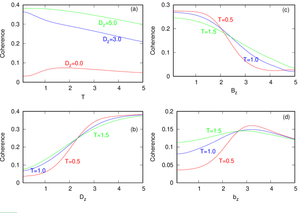
Figure 2: Measurement of coherence in the $\sigma_{z}$ basis in the two-spin XYZ model with DM interactions in the $z$-direction and the external magnetic field in the $z$-direction. (a) Quantum coherence versus temperature $T$ for different $D_{z}$, for $B_{z}=3.0$, $b_{z}=1.5$, $J_{x}=0.8$, $J_{y}=0.5$ and $J_{z}=0.2$. (b) Quantum coherence versus $D_{z}$ for different temperatures $T$, for $B_{z}=3.0$, $b_{z}=1.5$, $J_{x}=0.8$, $J_{y}=0.5$ and $J_{z}=0.2$. (c) Quantum coherence versus $B_{z}$ for different temperatures $T$, for $D_{z}=1.0$, $b_{z}=1.5$, $J_{x}=0.8$, $J_{y}=0.5$ and $J_{z}=0.2$. (d) Quantum coherence versus $b_{z}$ for different temperatures $T$, for $D_{z}=1.0$, $B_{z}=3.0$, $J_{x}=0.8$, $J_{y}=0.5$ and $J_{z}=0.2$.

The variation of quantum coherence as a function of the DM interaction and external field in the $\sigma_{z}$ basis is described through the plots in Fig. 2. The change of coherence with temperature is shown in Fig. 2(a) for different values of the DM interaction parameter. For larger values of the DM interaction parameter ($D_{x}=3.0,5.0$), we find that the quantum coherence decreases with temperature. This is in line with the observation in Ref. Li and Cao (2008) and the well known effect of thermal decoherene on quantum systems. For $D_{z}=0$, the coherence decreases but there is an initial increase. Through Fig. 2(b) we show the evolution of coherence with DM interaction. Quantum coherence increases with $D_{z}$ and this occurs for all values of temperature. The influence of magnetic field on quantum coherence is given in Figs. 2(c) and 2(d) for the homogeneous part and the inhomogenous part of the field respectively. In Fig. 2(c) we see that the quantum coherence decreases with the average homogeneous magnetic field $B_{z}$. From Fig. 2(d) we see that the coherence initially increases with the homogeneous field $b_{z}$, attains a maximum and then decreases to a saturation value.

In summary, in this section we considered the situation where the DM interaction and the external magnetic field are along the same direction. In both the cases the quantum coherence shows a decrease with temperature. When we look into the variation of quantum coherence with the DM interaction parameter, the average homogeneous magnetic field $B$, and the inhomogenous magnetic field $b$ we find that the measurement basis has a definite outcome on the value of quantum coherence. Hence the qualitative behavior of quantum coherence is quite different for the situations described in Sec. III A and Sec. III B and this is a unique feature of quantum coherence which does not have an analog in entanglement measurements.

IV DM interaction and the external field in different directions

In this section we consider the two-site XYZ model in which the spin-lattice interaction and the external field are in different directions. Under these conditions we have three different cases as follows: ($i$) The DM interaction is along the measurement basis; ($ii$) the external inhomogenous field is along the measurement basis and; ($iii$) both DM interaction and the external field are in different directions and orthogonal to the measurement basis. The coherence of all these cases are examined in the discussion below.

A $\vec{D}\propto\vec{z},\vec{B}\propto\vec{x}$ case

For the case with the DM interaction along the $z$-axis and the inhomogenous magnetic field along the $x$-axis, we have the Hamiltonian

$$H=J_{x}\sigma_{1}^{x}\sigma_{2}^{x}+J_{y}\sigma_{1}^{y}\sigma_{2}^{y}+J_{z}\sigma_{1}^{z}\sigma_{2}^{z}+D_{z}(\sigma_{1}^{x}\sigma_{2}^{y}-\sigma_{1}^{y}\sigma_{2}^{x})+(B_{x}+b_{x})\sigma_{1}^{x}+(B_{x}-b_{x})\sigma_{2}^{x}.$$ (30)

In the $\sigma^{z}$-basis the matrix form of the Hamiltonian is

$$H=\left(\begin{array}[]{cccc}J_{z}&-b_{x}+B_{x}&b_{x}+B_{x}&J_{x}-J_{y}\\ -b_{x}+B_{x}&-J_{z}&2iD_{z}+J_{x}+J_{y}&b_{x}+B_{x}\\ b_{x}+B_{x}&-2iD_{z}+J_{x}+J_{y}&-J_{z}&-b_{x}+B_{x}\\ J_{x}-J_{y}&b_{x}+B_{x}&-b_{x}+B_{x}&J_{z}\\ \end{array}\right).$$ (31)

From the Hamiltonian, one can calculate the density matrix $\rho(T)$ at thermal equilibrium. Using the thermal density matrix we can write down the diagonal form of the density matrix $\rho_{d}$ and using Eq. (6) we can calculate coherence in the system.

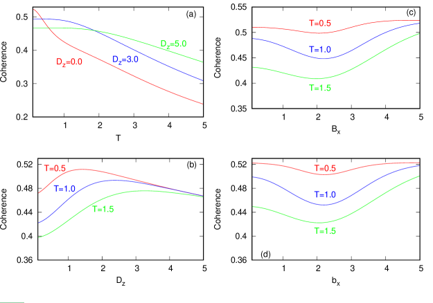
Figure 3: The change in coherence measured in the $\sigma_{z}$ basis for the two-site XYZ model with DM interactions in the $z$-direction and the external field in the $x$-direction. (a) Quantum coherence versus temperature $T$ for different $D_{z}$ for $B_{x}=3$, $b_{x}=1.5$, $J_{x}=0.8$, $J_{y}=0.5$ and $J_{z}=0.2$. (b) Quantum coherence versus $D_{z}$, for different temperatures $T$, for $B_{x}=3.0$, $b_{x}=1.5$, $J_{x}=0.8$, $J_{y}=0.5$ and $J_{z}=0.2$. (c) Quantum coherence versus $B_{x}$ for different temperatures $T$, for $D_{z}=1.0$, $b_{x}=1.5$, $J_{x}=0.8$, $J_{y}=0.5$ and $J_{z}=0.2$. (d) Quantum coherence versus $b_{x}$ for different temperatures $T$, for $D_{z}=1.0$, $B_{x}=3.0$, $J_{x}=0.8$, $J_{y}=0.5$ and $J_{z}=0.2$.

For this model, the variation of quantum coherence with the different parameters is shown in Fig. 3 with the measurement being carried out in the $\sigma_{z}$ basis. Thermal decoherence causes a loss of coherence due to increase in temperature and this is being observed in Fig. 3(a) for different strengths of the DM interaction. With respect to the DM interaction parameter, the coherence increases initially to attain a maximum value and then decreases. This behavior is shown in Fig. 3(b) for different temperatures. When the average homogeneous magnetic field $B_{z}$ is varied, the coherence decreases slightly to reach the minimum value and then increases back to a saturation value as shown in Fig. 3(c). A similar behavior is observed for the variation of the inhomogenous component of the field $b_{z}$ as seen in Fig. 3(d).

B $\vec{D}\propto\vec{x},\vec{B}\propto\vec{z}$ case

When the magnetic field is oriented along the $z$-axis and the DM interaction is along the $x$-axis, the Hamiltonian of the system reads:

$$H=J_{x}\sigma_{1}^{x}\sigma_{2}^{x}+J_{y}\sigma_{1}^{y}\sigma_{2}^{y}+J_{z}\sigma_{1}^{z}\sigma_{2}^{z}+D_{x}(\sigma_{1}^{y}\sigma_{2}^{z}-\sigma_{1}^{z}\sigma_{2}^{y})+(B_{z}+b_{z})\sigma_{1}^{z}+(B_{z}-b_{z})\sigma_{2}^{z}.$$ (32)

The matrix form in the $\sigma^{z}$ basis is

$$H=\left(\begin{array}[]{cccc}2B_{z}+J_{z}&iD_{x}&-iD_{x}&J_{x}-J_{y}\\ -iD_{x}&2b_{z}-J_{z}&J_{x}+J_{y}&iD_{x}\\ iD_{x}&J_{x}+J_{y}&-2b_{z}-J_{z}&-iD_{x}\\ J_{x}-J_{y}&-iD_{x}&iD_{x}&-2B_{z}+J_{z}\\ \end{array}\right).$$ (33)

The thermal density matrix $\rho(T)$ can be calculated from the Hamiltonian (33) using which we can find the quantum coherence of the system from Eq. (6).

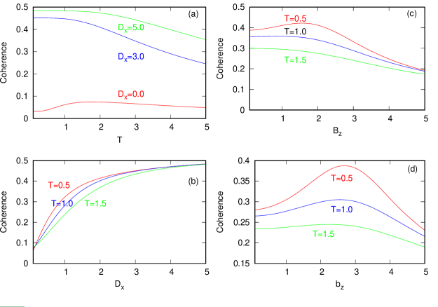
Figure 4: The variation in coherence is measured in the $\sigma_{z}$ basis for the two-spin XYZ model with DM interactions in the $x$-direction and the external magnetic field in the $z$-direction. (a) Quantum coherence versus temperatures $T$ for different $D_{x}$ for $B_{z}=3$, $b_{z}=1.5$, $J_{x}=0.8$, $J_{y}=0.5$ and $J_{z}=0.2$. (b) Quantum coherence versus $D_{x}$, for different temperatures $T$, for $B_{z}=3.0$, $b_{z}=1.5$, $J_{x}=0.8$, $J_{y}=0.5$ and $J_{z}=0.2$. (c) Quantum coherence versus $B_{z}$ for different temperatures $T$, for $D_{x}=1.0$, $b_{z}=1.5$, $J_{x}=0.8$, $J_{y}=0.5$ and $J_{z}=0.2$. (d) Quantum coherence versus $b_{z}$ for different temperatures $T$, for $D_{x}=1.0$, $B_{z}=3.0$, $J_{x}=0.8$, $J_{y}=0.5$ and $J_{z}=0.2$.

The dependence of quantum coherence with temperature is shown in Fig. 4(a). As before, we find that the coherence decreases with temperature as expected due to thermal effects removing coherence. With increase in the value of the DM interaction parameter, we find that quantum coherence increases monotonically as seen in Fig 4(b). From Fig 4(c) we can see that coherence decreases with the average homogeneous field $B_{z}$. While this is uniform for higher temperatures, for lower values of temperature the coherence increases to a peak value and then decreases. The same behavior is also replicated when we look into the variation of coherence with the inhomogenous field $b_{z}$ as seen in Fig. 4(d).

C $\vec{D}\propto\vec{x},\vec{B}\propto\vec{y}$ case

An interesting situation arises when the DM interaction and the external field are perpendicular to each other and neither of them are oriented along the measurement basis. The Hamiltonian in this case is

$$H=J_{x}\sigma_{1}^{x}\sigma_{2}^{x}+J_{y}\sigma_{1}^{y}\sigma_{2}^{y}+J_{z}\sigma_{1}^{z}\sigma_{2}^{z}+D_{x}(\sigma_{1}^{y}\sigma_{2}^{z}-\sigma_{1}^{z}\sigma_{2}^{y})+(B_{y}+b_{y})\sigma_{1}^{y}+(B_{y}-b_{y})\sigma_{2}^{y}.$$ (34)

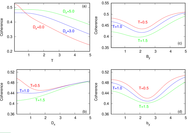
Figure 5: The coherence variation measured in the $\sigma_{z}$ basis for the XYZ model with DM interactions in the $x$-direction and the external field in the $y$-direction. (a) Quantum coherence versus temperature $T$ for different $D_{x}$ for $B_{y}=3$, $b_{y}=1.5$, $J_{x}=0.8$, $J_{y}=0.5$ and $J_{z}=0.2$. (b) Quantum coherence versus $D_{x}$, for different temperatures $T$, for $B_{y}=3.0$, $b_{y}=1.5$, $J_{x}=0.8$, $J_{y}=0.5$ and $J_{z}=0.2$. (c) Quantum coherence versus $B_{y}$ for different temperatures $T$, for $D_{x}=1.0$, $b_{y}=1.5$, $J_{x}=0.8$, $J_{y}=0.5$ and $J_{z}=0.2$. (d) Quantum coherence versus $b_{y}$ for different temperatures $T$, for $D_{x}=1.0$, $B_{y}=3.0$, $J_{x}=0.8$, $J_{y}=0.5$ and $J_{z}=0.2$.

From the knowledge of the Hamiltonian we can calculate $\rho(T)$ the thermal density matrix of the system and calculate the coherence using Eq. (6). Our results are shown in Figs. 5(a)-(d).

The quantum coherence decreases with temperature as seen in Fig. 5(a), as before due to thermal decoherence. The qualitative behavior of coherence with respect to change in the DM interaction parameter, the external homogeneous field $B_{z}$, and the inhomogeneous field $b_{z}$ is shown in Figs. 5(b), (c) and (d) respectively. The presence of spin-lattice interaction gives rise to new or enhanced contributions to off-diagonal elements and hence the overall effect is to increase the quantum coherence in the system. However in the XYZ model with both DM interaction and field in the $x$-direction, there is initially a decrease in coherence. After reaching the minimum the coherence again starts to increase. This dip occurs because the coherence arises due to two different interactions namely the spin-spin and the spin-lattice interaction. While the amount of coherence due to the spin-spin interaction decreases, the coherence due to the spin-lattice increases with the DM parameter $D_{x}$. There is a mismatch between the two rates of change leading to the formation of a dip in the amount of coherence. For higher values of temperature no dip is observed. In the case of the other two cases described in Sec. IV A and Sec. IV C, the coherence increases with $D_{x}$ for higher values of temperature. For lower values of temperature, the coherence decreases with DM parameter. This special behavior is also due to the competing rates of change of coherence of the spin-spin and spin-lattice interactions. Hence, overall we can conclude that coherence increases with the DM interaction, even if the effect may not be so easily observed.

In summary, when an external field is applied on a spin system, the field changes the quantum properties by influencing the spins. In our work, we study the effect of an inhomogenous external field. The external field can be divided into an homogeneous component $B$ and an inhomogenous component $b$. The strength and the direction of the homogeneous component $B$ of the field is the same for the spins at both the lattice sites. In the case of the homogeneous component $b$, the strength of the field acting on both the spins is the same, but their direction is different. From Figs. 1 - 5 we observe that the quantum coherence decreases when the direction of the homogeneous field $B$ is the same as the measurement basis. On the other hand, the coherence increases when the measurement basis and the external field are orthogonal to each other. In the case of the inhomogenous component of the field, the coherence mostly increases except for the isolated case of XYZ model with DM interaction along the $x$-direction and the field $b$ is along the $z$-direction.

V Coherence variation under two control parameters

Up to this point we have not considered the dependence of the spin-spin interaction $J_{i}$, which has been considered a constant. In this section, we examine the variation of coherence with respect to the simultaneous variation of the spin-spin interaction parameter and one of the other control parameters such as the DM parameter or the external field.

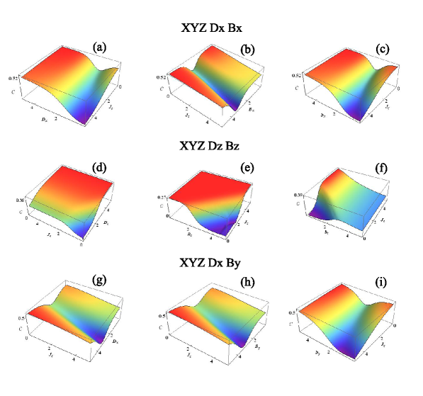
Figure 6: The variation of coherence in the XYZ model with DM interaction and external field along the $x$-axis is shown through the first row of plots as follows: (a) coherence Vs $J_{z}$ Vs $D_{x}$ (b) coherence Vs $J_{z}$ Vs $B_{x}$ (c) coherence Vs $J_{z}$ Vs $b_{x}$. The fixed values are $D_{x}=1.0$, $B_{x}=3.0$, $b_{x}=1.5$, $J_{x}=0.8$, $J_{y}=0.5$ and $T=0.5$. In the second row, the XYZ model with DM interaction and the field in the $z$-direction is given as follows: (d) coherence Vs $J_{z}$ Vs $D_{z}$ (e) coherence Vs $J_{z}$ Vs $B_{z}$ (f) coherence Vs $J_{z}$ Vs $b_{z}$. The fixed values are $D_{z}=1.0$, $B_{z}=3.0$, $b_{z}=1.5$, $J_{x}=0.8$, $J_{y}=0.5$ and $T=0.5$. The final row describes the XYZ model with DM interaction in the $x$-direction and the field along the $y$-direction as follows: (d) coherence Vs $J_{z}$ Vs $D_{x}$ (e) coherence Vs $J_{z}$ Vs $B_{y}$ (f) coherence Vs $J_{z}$ Vs $b_{y}$. The fixed values are $D_{x}=1.0$, $B_{y}=3.0$, $b_{y}=1.5$, $J_{x}=0.8$, $J_{y}=0.5$ and $T=0.5$. All the measurements are made uniformly in the $\sigma_{z}$ basis.

The quantum coherence in the two-spin XYZ model with DM interaction and the external field along the $x$-direction is described in the first row of plots in Figs. 6 (a)-(c). Fig. 6(a) shows the variation of coherence with respect to the spin-spin interaction parameter $J_{z}$ and the DM interaction parameter $D_{x}$. From the plot we observe that for a given a constant temperature, the amount of quantum coherence decreases with the spin-spin interaction parameter $J_{z}$. Contrarily on increasing $D_{x}$ the amount of coherence increases. This implies that the spin-spin interaction and the spin-lattice interaction have counteracting effects on the amount of coherence in the system. Fig. 6(b) shows the quantum coherence variation with respect to the parameters $J_{z}$ and $B_{x}$ (homogeneous component of the external field). Again we find that the coherence decreases with $J_{z}$, but increases with the external field. The external field $B_{x}$ tries to align the spins in a uniform direction and hence we observe an increase in the amount of quantum coherence. Fig. 6(c) shows coherence as a function of the spin-spin interaction $J_{z}$ and the inhomogenous component of the field $b_{x}$. This plot exhibits the features where we find that coherence decreases with $J_{z}$, whereas it increases with $b_{x}$. These observations are identical to the results obtained in Fig. 6(a) and 6(b).

In Figs. 6 (d)-(f) the quantum coherence features of the two-site anisotropic model with DM interaction and the field in the $z$-direction is shown. We choose the measurement basis also to be in the $\sigma_{z}$ basis and consider a constant temperature $T$. From Fig. 6(d) we find that the coherence increases with $J_{z}$ as well as $D_{z}$. In this situation, there is no counteracting influence between the spin-spin and spin-lattice interactions. Rather they exhibit a co-operative nature and enhances the coherence in the system with increase in these parameters. In Fig. 6(e) we notice that coherence decreases with increase in $B_{z}$ and it increases with $J_{z}$. Finally in Fig. 6(f) we observe that coherence increases with the inhomogenity of the external field $b_{z}$ as well with the increase of the spin-spin interaction parameter $J_{z}$.

Finally, in Figs. 6 (g)-(i) we look into the coherence dependence of the model with the spin lattice interaction in the $x$-direction and measurement along the $\sigma_{z}$ basis. The external inhomogenous field is along the $y$-direction. When the spin-spin interaction $J$ is increased, the coherence decreases. But when the spin lattice interaction is increased, the coherence increases. These results are shown in Fig. 6(g). Also through the plots Fig. 6(h) and Fig. 6(i) we find that coherence decreases with increase in the spin-spin interaction $J_{z}$. On increasing the homogeneous component $B_{y}$ and inhomogenous component $b_{y}$ we observe that the coherence increases.

In Table 1, based on the two dimensional plots, we summarize the variation of quantum coherence with different parameters for all the models. Using this in conjunction with Fig. 6 we arrive at the following conclusions. We find that when the direction of the DM interaction and external field is orthogonal to the measurement, the coherence in the system decreases with the spin-spin coupling $J$ value. Similarly, the coherence increases with the spin-lattice interaction parameter $D$. Also in this situation both the homogeneous and inhomogenous fields helps to increase the coherence in the system. Under the conditions when the direction of measurement basis is same as the direction of the spin-lattice, the spin-spin interaction and the DM interaction increases the quantum coherence in the system. With respect to the external field, the coherence decreases with increase in the homogeneous component of the field $B$ and it increases with the inhomogenous component of the field $b$.

Table 1: The variation of the coherences for the different parameters is summarized below. Here $+$ means coherence increases with the variable and $-$ means coherence decrease with the variable. The measurement basis is always in the $z$-direction.

Parameters	$\vec{D}\propto\vec{x}$	$\vec{D}\propto\vec{z}$	$\vec{D}\propto\vec{z}$	$\vec{D}\propto\vec{x}$	$\vec{D}\propto\vec{x}$
	$\vec{B}\propto\vec{x}$	$\vec{B}\propto\vec{z}$	$\vec{B}\propto\vec{x}$	$\vec{B}\propto\vec{z}$	$\vec{B}\propto\vec{y}$
Temperature $T$	$-$	$-$	$-$	$-$	$-$
DM interaction $D$	$+$	$+$	$+$	$+$	$+$
Homogeneous magnetic field $B$	$+$	$-$	$+$	$-$	$+$
Homogeneous magnetic field $b$	$+$	$+$	$+$	$-$	$+$

VI Conclusions

The finite temperature quantum coherence of the two-spin XYZ Heisenberg model with Dzyaloshinsky-Moriya (DM) interaction subjected to an external inhomogenous magnetic field was investigated. In the investigation of these two-site models we consider two major cases namely: ($i$) the DM interaction and the external magnetic field are in the same direction; ($ii$) when the DM interaction and the external field are not in the same direction. Since quantum coherence is a basis-dependent quantity, these two classes are further divided based on the relation between the measurement basis and the direction of the DM parameter and the field. We first confirm that quantum coherence always decreases with temperature, due to the commonly observed effect that quantum coherence is destroyed by thermal decoherence. Next we find that the quantum coherence always increases with the strength of the DM interaction parameter irrespective of the relation between the spin-lattice interaction and the measurement basis. This result is similar to the one obtained for entanglement measured using concurrence. The quantum coherence decreases when the direction of the measurement basis is the same as that of the spin-spin interaction. A similar behavior of quantum coherence is observed when the external field is varied.

A spin chain always contains a spin-spin interaction apart from the DM interaction and the external field as described in our work. We investigated the change in coherence when the spin-spin interaction is simultaneously varied with the DM interaction parameter or the external fields. From the observations we find that the spin-spin interaction and the spin-lattice interaction have counteracting effects on the quantum coherence of the system when the direction of the measurement is orthogonal to the direction of the spin-lattice interaction. We note that this study could be further extended to larger systems, and studying spin models with staggered DM interactions Ma et al. (2011); Miyahara et al. (2007) and random field interactions Bruinsma and Aeppli (1983); Fujinaga and Hatano (2007).

The amount and distribution of quantum coherence is connected to quantum information processing tasks like dense coding and quantum teleportation Pan et al. (2017). For example, the optimal dense coding capacity of a bipartite system is inversely related to the amount of local coherence in the system Pan et al. (2017). Similarly, there is an inverse relation between the teleportation fidelity and the local coherence in a system Pan et al. (2017). From our earlier studies Radhakrishnan et al. (2016) we know that coherence can exist localized within a qubit or as correlations between the qubits. Hence a small amount of local coherence must imply a higher amount of global coherence, which naturally means strongly correlated quantum systems help in tasks such as dense coding and quantum teleportation. In the case of the spin qubits considered, we observe that the total coherence in the system is always global coherence which implies that all the available form of coherence in a spin qubit can be used for quantum information processing tasks. In addition, the existence of several control parameters such as the spin-spin interaction parameter, the spin-lattice interaction parameter and the external parameters such as magnetic field and temperature helps us to modify the state of a system to improve the capacity of dense coding and the teleportation fidelity of quantum states. In Ref. Pan et al. (2017) the authors only demonstrated the complementarity relations of the local coherence with the dense coding capacity and the teleportation fidelity. An important development in this direction would be to directly quantify the dense coding capacity and teleportation fidelity in terms of the global coherence. Such an improvement will be directly applicable to the spin systems we have considered in our work, where we can quantify the ability to perform quantum information processing tasks using the coherence of the spin system.

References

- Glauber (1963) R. J. Glauber, Physical Review 131, 2766 (1963).
- Sudarshan (1963) E. Sudarshan, Physical Review Letters 10, 277 (1963).
- Baumgratz et al. (2014) T. Baumgratz, M. Cramer, and M. Plenio, Physical Review Letters 113, 140401 (2014).
- Yao et al. (2015) Y. Yao, X. Xiao, L. Ge, and C. Sun, Physical Review A 92, 022112 (2015).
- Yadin et al. (2015) B. Yadin, J. Ma, D. Girolami, M. Gu, and V. Vedral, arXiv preprint arXiv:1512.02085 (2015).
- Ma et al. (2016) J. Ma, B. Yadin, D. Girolami, V. Vedral, and M. Gu, Physical Review Letters 116, 160407 (2016).
- Yadin and Vedral (2016) B. Yadin and V. Vedral, Physical Review A 93, 022122 (2016).
- Bromley et al. (2015) T. R. Bromley, M. Cianciaruso, and G. Adesso, Physical Review Letters 114, 210401 (2015).
- Du et al. (2015) S. Du, Z. Bai, and Y. Guo, Physical Review A 91, 052120 (2015).
- Pires et al. (2015) D. P. Pires, L. C. Céleri, and D. O. Soares-Pinto, Physical Review A 91, 042330 (2015).
- Cheng and Hall (2015) S. Cheng and M. J. Hall, Physical Review A 92, 042101 (2015).
- Streltsov et al. (2015) A. Streltsov, U. Singh, H. S. Dhar, M. N. Bera, and G. Adesso, Physical Review Letters 115, 020403 (2015).
- Shi et al. (2017) H.-L. Shi, S.-Y. Liu, X.-H. Wang, W.-L. Yang, Z.-Y. Yang, and H. Fan, Physical Review A 95, 032307 (2017).
- Hillery (2016) M. Hillery, Physical Review A 93, 012111 (2016).
- Zhang et al. (2019) C. Zhang, T. R. Bromley, Y.-F. Huang, H. Cao, W.-M. Lv, B.-H. Liu, C.-F. Li, G.-C. Guo, M. Cianciaruso, and G. Adesso, Physical Review Letters 123, 180504 (2019).
- Ma et al. (2019) J. Ma, Y. Zhou, X. Yuan, and X. Ma, Physical Review A 99, 062325 (2019).
- Narasimhachar and Gour (2015) V. Narasimhachar and G. Gour, Nature Communications 6, 1 (2015).
- Winter and Yang (2016) A. Winter and D. Yang, Physical Review Letters 116, 120404 (2016).
- Brandão and Gour (2015) F. G. Brandão and G. Gour, Physical Review Letters 115, 070503 (2015).
- Chitambar and Hsieh (2015) E. Chitambar and M.-H. Hsieh, arXiv preprint arXiv:1509.07458 (2015).
- Chitambar and Gour (2016) E. Chitambar and G. Gour, Physical Review Letters 117, 030401 (2016).
- del Rio et al. (2015) L. del Rio, L. Kraemer, and R. Renner, arXiv preprint arXiv:1511.08818 (2015).
- Chitambar and Gour (2019) E. Chitambar and G. Gour, Reviews of Modern Physics 91, 025001 (2019).
- Radhakrishnan et al. (2016) C. Radhakrishnan, M. Parthasarathy, S. Jambulingam, and T. Byrnes, Physical Review Letters 116, 150504 (2016).
- Lostaglio et al. (2015) M. Lostaglio, D. Jennings, and T. Rudolph, Nature Communications 6, 1 (2015).
- Pan et al. (2017) F. Pan, L. Qiu, and Z. Liu, Scientific Reports 7, 43919 (2017).
- Georgescu et al. (2014) I. M. Georgescu, S. Ashhab, and F. Nori, Reviews of Modern Physics 86, 153 (2014).
- Opanchuk et al. (2016) B. Opanchuk, L. Rosales-Zárate, R. Teh, and M. Reid, Physical Review A 94, 062125 (2016).
- Zheng et al. (2016) Q. Zheng, J. Xu, Y. Yao, and Y. Li, Physical Review A 94, 052314 (2016).
- Ishida et al. (2013) N. Ishida, T. Byrnes, F. Nori, and Y. Yamamoto, Scientific reports 3, 1180 (2013).
- Karpat et al. (2014) G. Karpat, B. Çakmak, and F. Fanchini, Physical Review B 90, 104431 (2014).
- Lieb et al. (1961) E. Lieb, T. Schultz, and D. Mattis, Annals of Physics 16, 407 (1961).
- Niemeijer (1967) T. Niemeijer, Physica 36, 377 (1967).
- Niemeijer (1968) T. Niemeijer, Physica 39, 313 (1968).
- Barouch et al. (1970) E. Barouch, B. M. McCoy, and M. Dresden, Physical Review A 2, 1075 (1970).
- Barouch and McCoy (1971) E. Barouch and B. M. McCoy, Physical Review A 3, 786 (1971).
- Giamarchi (2004) T. Giamarchi, Quantum physics in one dimension (Oxford university press, 2004).
- Malvezzi et al. (2016) A. Malvezzi, G. Karpat, B. Çakmak, F. Fanchini, T. Debarba, and R. Vianna, Physical Review B 93, 184428 (2016).
- Li and Lin (2016) Y.-C. Li and H.-Q. Lin, Scientific Reports 6 (2016).
- Cheng et al. (2016) W. Cheng, Z. Zhang, L. Gong, and S. Zhao, The European Physical Journal B 89, 1 (2016).
- Çakmak et al. (2015) B. Çakmak, G. Karpat, and F. F. Fanchini, Entropy 17, 790 (2015).
- Radhakrishnan et al. (2017a) C. Radhakrishnan, I. Ermakov, and T. Byrnes, Physical Review A 96, 012341 (2017a).
- Dzyaloshinsky (1958) I. Dzyaloshinsky, Journal of Physics and Chemistry of Solids 4, 241 (1958).
- Moriya (1960) T. Moriya, Physical Review 120, 91 (1960).
- Wang (2001) X. Wang, Physical Review A 64, 012313 (2001).
- Zhou et al. (2003) L. Zhou, H. Song, Y. Guo, and C. Li, Physical Review A 68, 024301 (2003).
- Li and Cao (2008) D.-C. Li and Z.-L. Cao, The European Physical Journal D 50, 207 (2008).
- Kheirandish et al. (2008) F. Kheirandish, S. J. Akhtarshenas, and H. Mohammadi, Physical Review A 77, 042309 (2008).
- Li and Cao (2009) D.-C. Li and Z.-L. Cao, Optics communications 282, 1226 (2009).
- Gurkan and Pashaev (2010) Z. N. Gurkan and O. K. Pashaev, International Journal of Modern Physics B 24, 943 (2010).
- Guo et al. (2011) J.-L. Guo, Y.-J. Mi, J. Zhang, and H.-S. Song, Journal of Physics B: Atomic, Molecular and Optical Physics 44, 065504 (2011).
- Zidan (2014) N. Zidan, Journal of Quantum Information Science 2014 (2014).
- Yi-Xin and Zhi (2010) C. Yi-Xin and Y. Zhi, Communications in Theoretical Physics 54, 60 (2010).
- Radhakrishnan et al. (2017b) C. Radhakrishnan, M. Parthasarathy, S. Jambulingam, and T. Byrnes, Scientific Reports 7, 1 (2017b).
- Lin (1991) J. Lin, IEEE Transactions on Information theory 37, 145 (1991).
- Lamberti et al. (2008) P. Lamberti, A. Majtey, A. Borras, M. Casas, and A. Plastino, Physical Review A 77, 052311 (2008).
- Briët and Harremoës (2009) J. Briët and P. Harremoës, Physical Review A 79, 052311 (2009).
- Ma et al. (2011) F.-W. Ma, S.-X. Liu, and X.-M. Kong, Physical Review A 84, 042302 (2011).
- Miyahara et al. (2007) S. Miyahara, J.-B. Fouet, S. Manmana, R. Noack, H. Mayaffre, I. Sheikin, C. Berthier, and F. Mila, Physical Review B 75, 184402 (2007).
- Bruinsma and Aeppli (1983) R. Bruinsma and G. Aeppli, Physical Review Letters 50, 1494 (1983).
- Fujinaga and Hatano (2007) M. Fujinaga and N. Hatano, Journal of the Physical Society of Japan 76, 094001 (2007).