Emergent Hadrons and Diquarks

Abstract

We discuss the emergence of a low-energy effective theory with quarks, mesons, diquarks and baryons at vanishing and finite baryon density from first principle QCD. The present work also includes an overview on diquarks at vanishing and finite density, and elucidates the physics of transitional changes from baryonic matter to quark matter including diquarks. This set-up is discussed within the functional renormalisation group approach with dynamical hadronisation. In this framework it is detailed how mesons, diquarks, and baryons emerge dynamically from the renormalisation flow of the QCD effective action. Moreover, the fundamental degrees of freedom of QCD, quarks and gluons, decouple from the dynamics of QCD below the respective mass gaps. The resulting global picture unifies the different low energy effective theories used for low and high densities within QCD, and allows for a determination of the respective low energy constants directly from QCD.

I Introduction

There are a number of speculative scenarios for the large density phases of strongly interacting matter with quarks and gluons, see e.g. [1, 2, 3, 4, 5, 6, 7, 8, 9, 10, 11] for reviews. In QCD, only one of these many scenarios is singled out. However, it is still a tough problem to reduce uncertainties in theoretical treatments at finite baryon density.

In lattice-QCD, Monte-Carlo simulations break down for a baryon chemical potential comparable or larger than the temperature scale, $\mu_{\text{b}}/T\gtrsim 1$, see [12, 13, 14, 15, 16] for reviews on attempts to evade the sign problem.

By now, functional first principles approaches to QCD, such as the functional renormalisation group (fRG) approach or Dyson-Schwinger equations (DSEs), provide quantitative predictions for QCD correlation functions in the vacuum, at finite temperature, as well as moderate densities with baryon chemical potential $\mu_{\text{b}}$ restricted by $\mu_{\text{b}}/T\lesssim 4$, see [9, 10, 17, 18, 19, 20, 21].

Moreover, the fRG-approach allows to describe naturally the emergence of low energy effective theories (LEFTs) from first principle QCD: in this diagrammatic approach, off-shell quantum, thermal and density fluctuations are taken into account in terms of one-loop diagrams with full, momentum-dependent vertices and propagators. At lower momentum scales, gapped degrees of freedom successively decouple from the off-shell dynamics of the theory. Finally, at very low momentum scales, only the lowest lying degrees of freedom survive. For example, in vacuum QCD these are the pions. This picture of emergent low energy degrees of freedom and the decoupling of fundamentals ones, and in particular the gluons, already explains the success of chiral perturbation theory, or chiral effective theory ($\chi$EFT).

These processes and the dynamical emergence of the respective relevant degrees of freedom from QCD are naturally formulated with the functional renormalisation group approach: this approach allows the introduction of composite fields as dynamical degrees of freedom in the fundamental theory at hand. This is a very efficient reformulation of the fundamental theory in terms of dynamically relevant degrees of freedom. For example, if the latter completely dominate the dynamics of the theory, the fundamental degrees of freedom simply decouple. In turn, if either this dominance is not complete, or the composite fields are simply present as asymptotic states, the fundamental degrees of freedom still play a r$\hat{\textrm{o}}$le. This approach (rebosonisation or dynamical condensation) has been put forward in [22, 23], and has been further developed in [24, 25]. In QCD it is called dynamical hadronisation, for applications see [23, 26, 27, 28, 29, 10]. Its current form with further conceptual developments has been discussed in [10], for a recent review see [11].

Importantly, for smaller RG-scales the dynamics or RG-flows of full QCD resembles closely the RG-flow of low energy effective theories (LEFTs) with emergent hadronic and di-quark degrees of freedom, for a detailed discussion see [10, 11]. Such LEFTs have been studied intensively in the past decades, for QCD-related fRG reviews see [30, 24, 31, 32, 33, 34, 7, 11], a rather complete list of works can be found in [11].

However, while not hampered by a sign problem, at larger densities the reliability of the expansion order used so far in these functional works is successively lost. This is in one-to-one correspondence to an increasing numbers of potentially resonant hadronic interaction channels of multi-quark interactions, that have to be taken into account with dynamical hadronisation. While this is in principle possible systematically, it is still technically very challenging. Indeed, the present work will provide some of the necessary further developments of the expansion schemes.

Consequently, for large densities with $\mu_{\text{b}}/T\gtrsim 4$, this leaves us with the urgent task to device phenomenological studies within LEFTs, that can be systematically embedded into QCD. With the emergence of LEFTs from functional QCD via dynamical hadronisation, this systematics is provided. It is left to detail the relation of LEFTs to QCD, and to successively improve respective LEFTs via their connection to first principle QCD for $\mu_{\text{b}}/T\lesssim 4$ at present, but hopefully soon also larger densities. This leads to a very appealing situation with exciting possibilities: while LEFTs at large density can be benchmarked and improved systematically with their emergence (at lower densities) within first principle QCD for $\mu_{\text{b}}/T\lesssim 4$, phenomenological studies and improvements of LEFTs can guide the respective first principles studies. This combined analysis should allow to push the current $\mu_{\text{b}}/T\lesssim 4$ border further and further, finally resulting in a first principle access to QCD at all densities.

Note in this context, that LEFT-studies had played a similar guiding role in regimes with $T\gg\mu_{\text{b}}$, and many of the findings where later confirmed by lattice QCD or functional QCD studies. Naturally we expect that in the same way as for the high-$T$ studies, low energy effective field theory studies guide us to a correct intuition of the dense state of QCD matter.

Therefore, we proceed by discussing respective LEFTs used so far at large densities. We have already mentioned the emergence of $\chi$EFT within first principle QCD. Accordingly, a theoretical approach based on the chiral effective theory, see e.g. [35], should be a valid framework as long as the system is not far from cold nuclear matter, that is up to twice of normal nuclear density and temperature around the pion mass. Such a theoretical formulation in terms of hadronic degrees of freedom should be an alternative of the first principles approach based on the systematic low-energy expansion of QCD, but should lose its foundation at high density or high temperature where partonic degrees of freedom would become dominant. See also [36, 37] for a similar calculation using the renormalisation group equation based on [38], see also [39] for fluctuation estimate within the same model. More recently, the nuclear equation of state (EoS) has been investigated within the fRG, [40, 41], and in a combination of $\chi$EFT and fRG in QCD, see [42].

At moderate densities we may then investigate the properties of matter entirely out of quarks using the chiral quark models including fluctuations, for fRG work in this direction we refer to the reviews [30, 24, 31, 32, 33, 34, 7, 11], at asymptotically high densities much work has been done within (resummed) perturbative QCD calculations [43, 44, 45, 46], for respective fRG-work in QCD including deviations due to non-perturbative condensation effects see [42].

It is a big puzzle even today how these two descriptions of dense matter in terms of baryons and quarks could be (possibly smoothly [47, 48]) connected in an intermediate density region. In other words, there is no clear picture of quark deconfinement induced by large density effects, while deconfinement is a well-studied phenomenon along the temperature axis in lattice QCD and effective models. If we have a quark-model picture in mind, deconfinement simply means that bound states of quarks melt without phase transition [49] or the mobility of quarks gets increased by percolation [50], see also [51] for modernisation with quantum percolation. As we will argue later, such a picture should need more refinement taking account of differences between meson and baryon interactions.

A key ingredient to shed light on a modern picture of high-density deconfinement is the diquark correlation (see [52] for a comprehensive review on diquark physics). Diquarks form a condensate above the threshold, having an impact on the phase diagram. For example, see [53, 54] for a breach of the chiral phase boundary due to the diquark coupling. There are already some attempts to build an effective model in terms of diquarks as well as mesons and quarks (i.e., Quark-Meson-Diquark models). In conventional model set-ups as in [55] for example, it is common to accommodate diquarks as explicit (and point-like) degrees of freedom and generate baryons as bound states of quarks and diquarks [56, 57]. See also attempts [58, 59] in which diquark dissociation or the Mott transition has been taken into account, see [60, 61] for an application of the Quark-Meson-Diquark model for two-colour QCD, see [62] for fRG studies of an SO(6)-symmetric diquark model. Obviously, however, it is always possible to represent the baryon interpolation field as a combination of the diquark and the quark fields, see e.g. [63, 64] for its chiral properties. We emphasise that this does not entail the interpretation of diquarks as bound objects or asymptotic states. Clearly, they are not due to their colour. Instead, diquarks are dynamically generated (off-shell) excitations, and hence we must take into account these microscopic structures of diquarks.

We will formulate these processes of the formation and the dissociation of diquarks by means of the fRG equations. In this work we will give a theoretical foundation with correct physical degrees of freedom and physical boundary conditions satisfied. Here, we will limit ourselves to a rather simplified framework of the Lagrangian similar to the Quark-Meson-Diquark model. As we will explicitly see later, this simple framework is already nontrivial enough and needs technical developments beyond the simpler two-colour QCD case [60, 61, 65, 66].

In Section II we provide an overview on diquark constituents in hadrons and in dense quark matter. In Section III we discuss the continuous quark-hadron duality. In Section IV we iniate our analysis of emergent hadrons and diquarks with that on mesons and diquarks. In Section IV we iniate our analysis of emergent hadrons and diquarks with that on mesons and diquarks. It is shown, how resonant four-quark interaction channels in QCD can be described in terms of dynamical low energy degrees of freedom with dynamical hadronisation. In Section V this analysis is extended to baryons. This includes a discussion of the different formation processes of baryons via diquark-quark scattering and three-quark scattering. This analysis is continued in Section VI, specifically concentrating on quark-hadron mixing.

II Overview: Diquarks at Zero and Finite Baryon Density

Here we briefly review basic properties of diquarks in the contexts of hadronic structures and the ground state constituents in dense quark matter.

II.1 Classification of diquarks

The idea of the diquark can be traced back to a classic paper by Gell-Mann [67] and the word “diquark” was used already in a paper in 1966 [68] in the same way as we do today. It is a long-standing problem how to define diquarks, or precisely speaking, how to quantify diquark correlations in a baryon or in baryonic (nuclear) matter. In fact, it is a widely accepted knowledge to introduce a “constituent diquark” to solve a three-body bound state problem (i.e., the Faddeev equation) of baryons [69, *Ishii:1993rt, *Ishii:1995bu]. See also [72] for the two nucleon problem. The diquark in this formulation is, however, not necessarily a physical object and there are a number of theoretical attempts to seek for a strong and localised correlation of diquarks in hadrons.

One of the most well-known examples that suggest the diquark correlation is physical is the inverted mass ordering in the scalar nonet channel [73, *Jaffe:1976ih] and this idea is also supported by the instanton-induced interactions [75] (see [76] for a recent lattice study). There is also a proposal that some of the exotic $X$, $Y$, $Z$ mesons might have a significant overlap with the diquark–anti-diquark state on top of the meson molecule state (see [77] for an overview), though the coupled channel analysis with interactions from lattice QCD has clarified that $Z_{c}(3900)$ results from threshold enhancement [78]. Another example that indicates the diquark correlation is the $\Delta I=1/2$ rule in the non-leptonic weak decay, that is, the decay amplitude in the $\Delta I=1/2$ channel is by an order of magnitude enhanced than that in the $\Delta I=3/2$ channel. One possible interpretation for the $\Delta I=1/2$ rule is provided by the localised triplet-diquark in the hyperon wave-function that couples to the $\Delta I=1/2$ channel [79, 80, 81, 82, 83].

As diquarks are coloured objects, they do not exist as asymptotic states, and hence are not manifest observables in the vacuum. This leaves us with the physics question of whether diquarks exist as collective modes in some particular environments. In what follows below let us make a brief summary of a diquark classification in different channels.

Colour — Because quarks belong to the colour triplet, a system with two quarks can be decomposed to a colour anti-triplet and a sextet: (${\bf 3}_{c}\otimes{\bf 3}_{c}=\bar{\bf 3}_{c}\oplus{\bf 6}_{c}$). One-gluon exchange potentials suggest an attractive (and repulsive) force in the triple $\bar{\bf 3}_{c}$ (and sextet ${\bf 6}_{c}$, respectively) channel, so that we can discard colour ${\bf 6}_{c}$ pairing in the first approximation. In addition, it is only the $\bar{\bf 3}_{c}$ which can be coupled to another ${\bf 3}_{c}$ quark to form a colourless baryon.

Flavour — For $N_{f}=2$ two quarks can form ${\bf 2}_{f}\otimes{\bf 2}_{f}={\bf 1}_{f}\oplus{\bf 3}_{f}$ and for $N_{f}=3$ the irreducible decomposition reads as ${\bf 3}_{f}\otimes{\bf 3}_{f}=\bar{\bf 3}_{f}\oplus{\bf 6}_{f}$. For a given colour and flavour representation, the symmetry properties of the spin-orbit part is fixed by the Pauli principle. For instance, for a colour $\bar{\bf 3}_{c}$ and two-flavour ${\bf 1}_{f}$ or three-flavour $\bar{\bf 3}_{f}$, both colour and flavour indices are anti-symmetric under exchanging two quarks, and so the spin-orbit part of the diquark wave-function must be anti-symmetric to satisfy the Fermi statistics. Likewise a colour $\bar{\bf 3}_{c}$ and the symmetric two-flavour ${\bf 3}_{f}$ or three-flavour ${\bf 6}_{f}$ requires a spin-orbit part that is symmetric with respect to the exchange of two quarks.

Spin — The colour and flavour analysis above entails that the spin-orbit part should be anti-symmetric in the colour anti-symmetric and flavour anti-symmetric channel, and the allowed quantum numbers are $0^{+}$ (for $L=0$, $S=0$), $1^{-}$ (for $L=1$, $S=0$), etc. If the colour is anti-symmetric and the flavour is symmetric, on the other hand, the spin-orbit part should be also symmetric. Then, $1^{+}$ (for $L=0$, $S=1$), $0^{-}$ (for $L=1$, $S=1$), etc. should appear.

It is chromo-magnetic interaction that favours positive-parity (i.e., $0^{+}$ and $1^{+}$) diquarks rather than negative-parity (i.e., $0^{-}$ and $1^{-}$) ones. Moreover, it is straightforward to confirm that the colour-spin and flavour-spin interaction would stabilise the $0^{+}$ diquark more, which is concisely dictated by the Breit interaction in QCD proportional to the inner product of two spins, $(\bm{s}_{1}\cdot\bm{s}_{2})$. For the spin singlet state $(\bm{s}_{1}\cdot\bm{s}_{2})$ takes a value of $-3/4$, while it is $+1/4$ for the spin triplet state, leading to an energy difference between $0^{+}$ and $1^{+}$. Thus, the $0^{+}$ scalar diquark called “good diquark” is the most favoured, and the $1^{+}$ axial-vector diquark called “bad diquark” is the second favoured. It is important to distinguish the good and the bad diquarks for phenomenological applications; see, for example, [84] for high-spin hadron spectra nicely parametrised with the good and the bad diquarks.

Since diquarks are not gauge invariant, it is indispensable to choose a certain gauge to observe diquarks in the lattice-QCD simulation. (This is the biggest difference from diquarks in two-colour QCD, where diquarks are colourless baryons [85, 60].) In Ref. [86] the diquark mass has been estimated in lattice-QCD (with $m_{\pi}\simeq 350\;\text{MeV}$) to be $m_{\text{good}}=694(22)\;\text{MeV}$ from the exponential decay in the diquark-diquark correlation, and also an expected relation of the mass difference between $S=1$ and $S=0$ channels, i.e. $m_{\text{bad}}-m_{\text{good}}\approx\frac{1}{2}(m_{\Delta}-m_{\text{N}})$, was investigated. Here, $m_{\text{good}}$ and $m_{\text{bad}}$ represent the masses of the good diquark in the scalar channel and the bad diquark in the axial-vector channel. Also the maximum entropy method has been applied to calculate the diquark spectral functions [87] and a prominent peak stands at the diquark mass $m_{\text{good}}=0.60(2)\;\text{GeV}$. Interestingly, the spatial size of the diquark correlation in a hadron has been also evaluated from the charge or baryon density distribution measured on the lattice [88, 89]. The characteristic size of the diquark correlation which is the strongest in the $0^{+}$ channel is, however, found to be comparable to the hadron size $\sim 1\;\text{fm}$. Therefore, it is definitely true that the diquark “correlation” exists inside of baryons (or even more manifested in systems of one heavy quark and two light quarks [90]), but diquarks do not necessarily appear as point-like particles but they should look like spatially extended objects. It is important to keep in mind that diquarks could be extended objects and this is why we need to solve a dynamical problem to treat diquarks as emergent degrees of freedom.

II.2 Diquarks in colour superconductivity

The fact that diquarks are not point-like is evident in the consideration of colour superconductivity that is a ground state of QCD matter at asymptotically high density [91, 92], for reviews see [3, 1, 2]. Among various pairing patterns [93, 94], the two-flavour colour superconducting (2SC) phase and the colour-flavour locked (CFL) phase, which are both characterised by condensation of the good diquarks, have special importance on the phase diagram of high-density matter [95]. Also for one-flavour colour superconductivity, the flavour sector is symmetric and so only the bad diquark is possible. Then, the rotational symmetry is broken by condensation of axial-vector diquark, leading to a spin-one colour superconductivity [96].

The 2SC phase should be a ground state if the $s$-quark mass is sufficiently large. This state, however, does not break global ${\rm U(1)_{V}}$ symmetry and so it is not a superfluid. Moreover one can prove that chiral symmetry is not broken in the 2SC phase; anti-symmetric combination of two ${\bf 2}_{f}$ forms a flavour singlet. Therefore, if there is an interface between the hadronic phase and the 2SC phase, there should be a chiral phase transition. There is also a possibility of a coexisting state of the 2SC gap and the chiral condensate that breaks chiral symmetry. Besides, a mixture of spin-one and tensorial diquark condensates may be possible, and then it is difficult to distinguish baryonic matter (in which $\langle pp\rangle\sim\langle uuudud\rangle$ and $\langle nn\rangle\sim\langle ddudud\rangle$ pairings exist) from the 2SC phase (with $\langle ud\rangle$ in the colour-triplet channel and $\langle uu\rangle$ and $\langle dd\rangle$ in the colour-sextet channel) from the symmetry arguments not only for ${}^{1}S_{0}$ but also ${}^{3}P_{2}$ states, see [48].

The CFL phase is also indistinguishable from baryonic matter with strangeness superfluid components. Unlike the 2SC phase the CFL phase itself spontaneously breaks chiral symmetry and ${\rm U(1)_{V}}$ symmetry associated with superfluidity [97]. So, all of ${\rm U(3)_{L}\times U(3)_{R}}$ symmetry in flavour space is broken by the condensates. It has been an established knowledge that the chiral symmetry breaking is partially restored at normal nuclear density about $\sim 30\%$ (see Ref. [98] and references therein), but there is so far no convincing evidence for full chiral restoration [99]. In fact, contrary to our naive intuition of symmetry restoration at higher density, once the CFL phase occurs, chiral symmetry must be always broken even at high baryon densities. Interestingly, physical degrees of freedom may have one-to-one correspondence between baryonic and quark matter [100, 101, 53]; for example, mesons in the hadronic phase are composed from a quark and an anti-quark, while in the CFL phase mesons are mostly tetra-quark objects of a diquark and an anti-diquark [102] just like the hypothesised nonet scalar mesons. The counterparts of baryons in the hadronic phase are quarks in the CFL phase. Recently, the continuity in terms of superfluid vortices has also been studied; some arguments disfavour the continuity [103, 104], and others support the continuity [105, 106].

For both cases of the 2SC phase and the CFL phase, the important point is that a scenario with no first-order phase transition between baryonic matter and quark matter can be a logical possibility. In other words, baryonic and quark matter is indistinguishable, in principle, from the symmetry (and also from the topology, see [106]). On the formal level, such a hypothesis of the Quark-Hadron Continuity is based on the fact that there is no gauge invariant order parameter to define colour superconductivity. In lattice-QCD simulation or in any experimental measurements what we can observe is an expectation value of gauge-invariant operators. Then, the 2SC and the CFL phases could be characterised by condensation of four-quark and six-quark operators, but these quantities would be non-vanishing already in baryonic matter with a superfluid component.

III Continuous Duality Between Baryonic And Quark Matter with Diquarks

We know that at zero temperature the first onset of baryon density appears with a first-order phase transition from vacuum to normal and symmetric nuclear matter as the baryon chemical potential $\mu_{\text{b}}$ increases. It happens at $\mu_{\text{b}}=M_{\text{N}}-\epsilon_{B}\simeq 923\;\text{MeV}$ for symmetric nuclear matter, where $M_{\text{N}}\simeq 939\;\text{MeV}$ is the nucleon mass and $\epsilon_{B}\simeq 16\;\text{MeV}$ is the binding energy. Right on the phase transition, a mixed state realises and various spatial structures may occur [107]. The question is where we can expect other degrees of freedom of quarks and diquarks.

III.1 From a bag model picture to a modern view

If there are any new degrees of freedom in matter coupled to the baryon density, it would emerge when the baryon chemical potential exceeds the corresponding mass threshold. If density-induced deconfinement is a smooth phenomenon just as observed along the temperature axis, as argued in the previous section, confinement would be gradually lost in baryonic matter. Then, the quark onset should be located at three times the (in-medium) constituent quark mass (if the interaction effect is renormalised in the effective mass). In the same way, as soon as $\mu_{\text{b}}$ gets greater than three halves times the (in-medium) constituent diquark mass, the system should accommodate the diquark degrees of freedom. We should note that the diquarks immediately form a condensate because they are bosons, leading to a colour superconducting state. So, the onset of diquarks degrees of freedom is essentially the onset of colour superconductivity.

The old-fashioned picture of deconfinement is as follows. The pressure of quark matter, $P_{\text{deconfined}}$, and the pressure of baryonic matter, $P_{\text{confined}}$, are compared and the one with larger pressure is identified as the favoured state. In this bag model picture physical degrees of freedom are switched sharply at the density with $P_{\text{deconfined}}=P_{\text{confined}}$. In this picture the double-counting problem of relevant physical degrees of freedom is avoided too strongly, and any coexistence of baryons, quarks, and diquarks is excluded by construction.

In a dynamical picture which allows for smooth dissociation of bound states, however, coexistence is not excluded, and it would be a natural anticipation to consider successive onsets. For the ensuing discussion let us introduce some notations here; the constituent quark mass is denoted by $M_{\text{q}}$, the constituent diquark mass by $M_{\text{d}}$, the baryon binding energy by $\epsilon_{N}$, the diquark mass difference by $\epsilon_{d}$, so that $M_{\text{N}}=3M_{\text{q}}-\epsilon_{N}$ and $M_{\text{d}}=2M_{\text{q}}-\epsilon_{d}$, where $\epsilon_{N}>0$ and $\epsilon_{d}<0$ supposedly. Then, we have an ordering pattern as $M_{\text{N}}<3M_{\text{q}}<\frac{3}{2}M_{\text{d}}$. We postulate $\epsilon_{d}<0$ because the diquark shows up not as a bound state in configuration space but as a correlation in momentum space.

If the diquark correlation is strong enough, there is a possibility of diquarks being localised bound states with $\epsilon_{d}>0$. In this case one might think that bound diquarks appear earlier than quarks, but because of the gap, the quark energy dispersion relation is modified. Then, there is no longer a sharp Fermi surface of quarks even at zero temperature, and the onset of quarks is blurred. We should consider that the onset of quarks is thus determined by the onset of diquarks in this case. Besides, diquarks in QCD are coloured objects and strongly interacting. Therefore, it is not clear whether there is any sharp onset of such interacting diquarks, which also underlies the idea of the Quark-Hadron Continuity.

III.2 A further push – continuous duality

The large-$N_{\mathrm{c}}$ (where $N_{\mathrm{c}}$ is the number of colours) approximation for QCD matter provides us with interesting pictures that are more or less consistent with the above. There may be no particular onset behaviour of quarks and diquarks but these degrees of freedom may be gradually developing as the baryon density grows up. In other words, in the large-$N_{\mathrm{c}}$ world, interacting nuclear matter and quark matter share the same properties. This is the state-of-the-art understanding of dense QCD matter as Quarkyonic Matter recognised in [108]. The baryons interact as strongly as $\sim\mathcal{O}(N_{\mathrm{c}})$ enhanced by a combinatorial factor due to quark exchanges, while mesons become free particles when $N_{\mathrm{c}}$ is infinitely large. Thus, interestingly, baryon interactions lead to the same $N_{\mathrm{c}}$ counting as quark matter and so quark degrees of freedom should be already there through baryon interactions. The duality between nuclear matter and quark matter is seemingly a radical interpretation of the large-$N_{\mathrm{c}}$ observation, but we emphasise that such a quarkyonic picture is very natural. The baryon interaction is mediated by mesons which are objects of a quark and an anti-quark. So, by this interaction, quarks can hop from one baryon to the other, and this is nothing but a mobility characterisation of deconfinement at large densities. The traditional picture in nuclear physics is composed of baryons with meson exchanges, which may well be regarded as partial deconfinement by quark exchanges, see soft deconfinement arguments in [51].

To implement such continuous duality in the field-theoretical calculation, we should deal with hadrons, diquarks, and quarks in a way without the double-counting problem, and also we should ensure the correct boundary condition that degrees of freedom at ultraviolet (UV) scale should be quarks and gluons only, which are the subjects we are discussing in the following sections.

IV Emergent mesons and diquarks

In the following two sections, Section IV and Section V, we discuss how hadrons emerge as dynamical degrees of freedom in the low energy regime of QCD. One illuminating setting for emergent degrees of freedom is the functional renormalisation group, fRG, approach, where the theory is solved in an iterative procedure by reducing a flowing energy or momentum scale from the initial perturbative UV energy scales down to non-perturbative infrared (IR) energy scales. Within such a procedure dynamical low energy degrees of freedom emerge as resonant interaction channels. Hadrons, as well as diquarks can be identified by the quantum numbers of the interaction channels under investigation. The introduction of effective degrees of freedom for the respective channel interactions turns out to be a very efficient book-keeping device [22, 23, 24, 25] for general condensation phenomena. This procedure is called dynamical hadronisation. As indicated above, it accounts for the dynamical adjustment of the physical degrees of freedom of the theory at the flowing energy scale $k$.

IV.1 QCD flows

By now, the fRG approach to QCD is a well-established formalism for computing correlation functions by integrating momentum fluctuations out from a UV scale, $\Lambda\gg\Lambda_{\text{\tiny QCD}}$, down toward an IR scale. See [7, 27, 26, 28, 109, 29, 110, 111, 10] for recent quantitative works in Yang-Mills theory and QCD. The master flow equation for the effective action of QCD including dynamical hadronisation is given by [10]

$$\left(\partial_{t}+\partial_{t}\Phi_{i,k}[\Phi]\frac{\delta}{\delta\Phi_{i}}\right)\left(\Gamma_{k}[\Phi]+c_{\Phi_{i}}\Phi_{i}\right)$$

$$= \,\frac{1}{2}{\rm Tr}\,G_{A}[\Phi]\partial_{t}R_{A}-{\rm Tr}\,G_{c}[\Phi]\partial_{t}R_{c}-{\rm Tr}\,G_{q}[\Phi]\partial_{t}R_{q}$$

$$\,+\frac{1}{2}{\rm Tr}\,G_{\phi}[\Phi]\partial_{t}R_{\phi}+\frac{1}{2}{\rm Tr}\,G_{d}[\Phi]\partial_{t}R_{d}-{\rm Tr}\,G_{b}[\Phi]\partial_{t}R_{b}\,,$$ (1)

where the effective action contains linear terms in $\Phi_{i}$. These terms generically occur in the presence of explicit chiral symmetry breaking. In their absence the effective action is that in the chiral limit, for a details discussion see [10]. Accordingly, the combination $\Gamma_{k}[\Phi]+c_{\Phi_{i}}\Phi_{i}$ does not contain terms linear in the $\Phi_{i}$, and the flow of the theory in the presence of explicit chiral symmetry breaking is that of the chirally symmetric one in the chiral limit. The flow Equation 1 is schematically depicted in Figure 1, see [7, 10, 11] for an overview.

The $t$-derivative on the right hand side where $\partial_{t}=k\partial_{k}$ is taken at fixed field $\Phi$ which encodes all fields, $\Phi=(A\,,\,c\,,\,\bar{c}\,,\,q\,,\,\bar{q}\,,\,\sigma\,,\,\vec{\pi}\,,\,d\,,\,d^{*}\,,\,\bar{b}\,,b,\ldots)$. The field derivative term on the left hand side relates to dynamical hadronisation, and its occurrence is detailed in Section IV.4. The standard flow equation for QCD is obtained, when dropping the dynamical rebosonisation terms that come with the introduction of effective low energy fields. Then, QCD is solely described in terms of gluons, ghosts and quarks. Then, on the left hand side of Equation 1 only the $\partial_{t}\Gamma_{k}$ term is present, and only the loops of the fundamental degrees of freedom survive on the right hand side: the third line in Equation 1 disappears. In Figure 1 this simply amounts to dropping the third line.

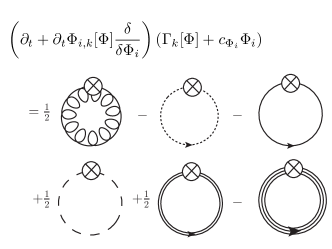
Figure 1: Flow equation for the effective action of QCD. The lines stand for the full propagators of gluons, ghost, quarks, and hadronic degrees of freedoms, the crossed circle stands for the cutoff insertion, see Equation 1. The loops encode the contributions of fluctuations of gluons, ghost, quarks, and hadrons introduced by dynamical hadronisation.

Flow equations for correlation functions are then obtained by taking derivatives with respect to the fields. Figure 1 is a one-loop exact differential equation, where each loop encodes the fluctuation effect of gluons, ghosts, quarks, and also that of collective degrees of freedom with hadronic quantum numbers. The propagators in the loops are taken in general background fields $\Phi$, and the loops are peaked at momenta $p$ about a sliding momentum scale $p^{2}\approx k^{2}$ due to the cutoff insertion $\partial_{t}R_{\Phi}(p)$. The second line encodes the off-shell fluctuations of the fundamental degrees of freedom, gluons, ghosts and quarks. The third line encodes that of hadronic degrees of freedom, in the present case the lightest scalar and pseudoscalar mesons, i.e., $\phi=(\sigma,\vec{\pi})$, and the lightest baryons, i.e., the nucleons $b$. Finally we also include collective modes of the diquarks $d$ in the present case.

We emphasise that the hadronic and collective mode contributions in Figure 1 do not signal an effective model approach but rather stand for an efficient book-keeping of resonant channels of multi-quark interactions. This procedure, called dynamical hadronisation or rebosonisation [22, 23, 24, 25], has been extended further in the case of mesons in [27, 26] (see a review [112] and references therein for application to molecules and trimers). In the present work we generalise the approach to diquark and baryon channels in four-quark and six-quark interactions, respectively.

The local composite operators in this work, i.e., $\Phi_{i}=\sigma,\,\vec{\pi},\,d,\,b$ carry the quantum numbers of mesons, diquarks, and baryons, respectively. They are introduced via one-meson, one-diquark, and one-baryon exchanges, taking care of specific momentum channels (with the coupling $\lambda_{\Phi_{i}}$) of four-quark and six-quark scattering vertices. Due to the single-particle exchange relation amplitudes in these channels read $|\lambda_{q\phi/d}|\propto h_{q\phi/d}^{2}/m_{\phi/d}^{2}$ for mesons and diquarks, and $|\lambda_{b}|\propto h_{qdb}^{2}/m_{b}^{2}$ for baryons at vanishing exchange momentum. This is detailed in Section IV.3. Here $m_{\phi/d/b}$ is the mass gap of the meson/diquark/baryon dispersion, and $h_{q\phi/d}$ or $h_{qdb}$ is the Yukawa coupling between a $\bar{q}q$ (meson), a $qq$ (diquark), or a $qd$ (baryon) and the respective composite fields. Hence, decreasing multi-quark scattering amplitudes in the UV region simply implies that corresponding states acquire mass-type dispersions with increasing masses (at fixed Yukawa coupling) at large momentum scales. Note in this context that also chiral channels can acquire a mass gap in the above sense.

We expect that within the present approach we smoothly flow from high energy QCD with quarks and gluons toward low energy QCD with dynamical quarks and hadrons. The low energy degrees of freedom get potentially dynamical at about the chiral symmetry breaking scale, $k_{\chi}\approx 0.5-0.4\;\text{GeV}$. Evidently, for $k<k_{\chi}$, only the lowest-lying mesons of $(\sigma,\vec{\pi})$ can contribute to the loops. Hence, we expect semi-quantitative results already with an approximation with dynamical gluons, quarks, and $(\sigma,\vec{\pi})$ at least at vanishing chemical potential. In turn, asymptotic states have to include higher meson multiplets and baryons. Nevertheless, diquarks may play a role in the baryon formation and should be taken into account especially at finite density, though they are not asymptotic states as not being colourless.

IV.2 The effective action at large momentum scales

At a large flowing scale $k\gg\Lambda_{\text{\tiny QCD}}$ the effective action $\Gamma_{k}$ is well-described by the classical (finite) action of QCD as

$$\Gamma_{k\gg\Lambda_{\text{\tiny QCD}}}\simeq \int_{x}\;\biggl{\{}\frac{1}{4}F^{a}_{\mu\nu}F^{a}_{\mu\nu}+\bar{q}\Bigl{(}\not{D}+m_{q}\Bigr{)}q$$

$$\qquad\quad+\bar{c}^{a}\partial_{\mu}D^{ab}_{\mu}c^{b}+\frac{1}{2\xi}(\partial_{\mu}A_{\mu}^{a})^{2}\biggr{\}}\,,$$ (2)

with covariant derivative $D_{\mu}=\partial_{\mu}-igA_{\mu}^{a}t^{a}$, and $\int_{x}=\int d^{4}x$. Here we have normalised the fields and couplings such that wave-function renormalisations and coupling renormalisations can be taken to be unity at the given scale. In the present approach the UV effective action also features a gluon mass term due to the cutoff term that leads to modified Slavnov-Taylor identities. This mass term has to vanish for vanishing cutoff scale, and we suppress it in the following qualitative discussion (for more details see [109] and references therein). The quark mass $m_{q}$ is the running current quark mass in the present fRG scheme.

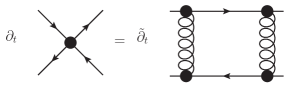
Figure 2: Generation of four-quark couplings in the first RG-step via the gluonic box diagram (permutations, signs, and diagram multiplicities are not shown). The derivative $\tilde{\partial}_{t}$ only hits the explicit $t$-dependence in the regulators of the involved propagators.

Inserting the UV-effective action Equation 2 into the right hand side of Equation 1 generates all-order scattering terms within one RG-step. The flow of the corresponding vertices,

$$\Gamma^{(n)}_{\Phi_{1}\cdots\Phi_{n},k}(p_{1},\ldots,p_{n-1})=\int_{p_{n}}\frac{\delta^{n}\Gamma_{k}[\Phi]}{\delta\Phi_{1}(p_{1})\cdots\delta\Phi_{n}(p_{n})}\,,$$ (3)

can be obtained by taking the derivatives of Equation 1 with respect to the fields, $\Phi_{1},\dots,\Phi_{n}$. The integral $\int_{p_{n}}=\int d^{4}p_{n}/(2\pi)^{4}$ on the right hand side of Equation 3 simply eliminates $(2\pi)^{4}\delta(p_{1}+\cdots+p_{n})$ that signals momentum conservation, and $p_{n}=-(p_{1}+\cdots+p_{n-1})$ is understood on the left hand side. Now we use this structure for the four-quark interactions. A flow step towards lower cutoff scales, $k\to k-\Delta k$, immediately generates momentum-dependent four-quark interaction terms as depicted in Figure 2. The diagram on the right hand side of Figure 2 is the only contribution to the four-quark flow if we insert the UV-effective action Equation 2 on the right hand side of Equation 1. The four-quark term on the left hand side of Figure 2 includes all possible four-quark tensor structures that are not forbidden by the symmetry properties of the flow as well as the symmetry properties of the initial effective action Equation 2. Hence, these terms have to be added to the effective action Equation 2. Concentrating only on purely fermionic terms this reads very schematically

$$\Gamma_{k}\simeq \,\Gamma_{k\gg\Lambda_{\text{\tiny QCD}}}+\Gamma_{\bar{q}q\bar{q}q,k}+O(1/k^{3})\,,$$

$$\Gamma_{\bar{q}q\bar{q}q,k}[\bar{q},q]= \,\frac{1}{4}\int_{p_{1},p_{2},p_{3}}\bar{q}_{p_{1}}q_{p_{2}}\bar{q}_{p_{3}}\bar{q}_{p_{4}}\Gamma^{(4)}_{\bar{q}q\bar{q}q,k}(p_{1},\ldots,p_{3})\,.$$ (4)

In Equation 4 the internal spinor and group indices are suppressed and momentum conservation $p_{4}=-(p_{1}+p_{2}+p_{3})$ is implied. The vertex function $\Gamma^{(4)}_{\bar{q}q\bar{q}q}(p_{1},\ldots,p_{3})$ carries all tensor structures allowed by symmetries; for $N_{f}=2$ the complete Fierz basis includes 10 tensor structures (at vanishing momentum). Here we used a common basis also used in [27]. For more details see Appendix A. Note that at large cutoff scales the four-quark terms are irrelevant. For dimensional reasons they run with $1/k^{2}$. Moreover, $\Gamma^{(4)}_{\bar{q}q\bar{q}q,k}(p_{1},\ldots,p_{3})\propto\alpha_{s,k}^{2}$ with $\alpha_{s,k}=g_{k}^{2}/(4\pi)$, which follows straightforwardly from the flow in Figure 2. In the same way higher fermionic interaction terms are generated as well as general quark-gluon interaction terms. At large momentum scales all these terms are even more suppressed by powers of the cutoff scale and the running strong coupling $\alpha_{s,k}$ due to perturbative power-counting.

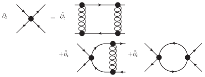
Figure 3: Schematic representation of the flow equation for the four-quark coupling involving just QCD degrees of freedom (permutations, signs, and diagram multiplicities are not shown). The derivative $\tilde{\partial}_{t}$ only hits the explicit $t$-dependence in the regulators of the involved propagators.

For now let us concentrate on the four-quark terms, and drop the other perturbatively irrelevant terms for the current qualitative argument. Furthermore we go to the chiral limit. The four-quark couplings generate further diagrams in their flow equation, as well as in the flows of other couplings. In the approximation indicated in Equation 4 the full flow of $\Gamma^{(4)}_{\bar{q}q\bar{q}q,k}(p_{1},\ldots,p_{3})$ is now given by terms as shown in Figure 3. Again the perturbative ordering is extracted straightforwardly: the last two diagrams with two and one four-quark coupling are proportional to $\alpha_{s,k}^{4}$ and $\alpha_{s,k}^{3}$, and hence are suppressed by additional powers of the coupling in comparison to the first quark-gluon diagram.

IV.3 Resonant interactions and low energy degrees of freedom

Here we discuss dynamically emergent mesons and emergent diquarks.

IV.3.1 Emergent scalar-pseudoscalar mesons

When the cutoff scale approaches the hadronisation scale $k_{\text{\tiny{had}}}\approx 0.5\;\text{GeV}$, the four-quark interaction gets resonant at least for the scalar-pseudoscalar tensor structure with the pion ($\vec{\pi}$) and sigma ($\sigma$) quantum numbers. Within a Fierz-complete basis given in Appendix A the scalar-pseudoscalar tensor structure can be read off from the Lagrangian which is for $N_{f}=2$ given by

$$\mathcal{L}_{(\bar{q}q)^{2}}^{(\phi)} =-\frac{\lambda_{q\phi}}{2}Z_{q}^{2}\left[(\bar{q}q)^{2}-(\bar{q}\gamma^{5}\vec{\tau}q)^{2}\right]$$

$$=-\frac{\lambda_{s}}{2}Z_{q}^{2}\,\bar{q}^{\bar{\bm{a}}_{1}}q^{\bm{a}_{1}}\bar{q}^{\bar{\bm{a}}_{2}}q^{\bm{a}_{2}}\,T_{\rm s}^{\bar{\bm{a}}_{1}\bm{a}_{1}\bar{\bm{a}}_{2}\bm{a}_{2}}\,,$$ (5)

where bold indices, $\bm{a}_{i}$ and $\bar{\bm{a}}_{i}$, run over Dirac, colour and flavour indices. For the embedding of $T_{\rm s}^{\bar{\bm{a}}_{1}\bm{a}_{1}\bar{\bm{a}}_{2}\bm{a}_{2}}$ in the complete Fierz basis used here see also Equation 90. Now we restrict ourselves to a subspace of full momentum space that is parametrised by only two momentum variables. A distinguished choice is a channel with vanishing momentum of the diquark, where the sum of both (anti)quark momenta vanishes, see Figure 4. This momentum condition is given by $(p_{1}+p_{3})^{2}=(p_{2}+p_{4})^{2}=0$ or $p_{1}=q=-p_{3}$ and $p_{2}=-q+p=-p_{4}$, where $p$ is the exchange momentum. This can be interpreted as projecting the scalar-pseudoscalar tensor structure on collective $q\bar{q}$ –mesonic– degrees of freedom. This suggests to rewrite the full scalar-pseudoscalar four-quark interaction for vanishing momentum in the diquark channel into $\Gamma_{\bar{q}q\bar{q}q,k}^{(4),(\phi)}$ in terms of an exchange of effective $SU(2)$-flavour field $\phi=(\sigma,\vec{\pi})$ with the $\sigma$ and $\vec{\pi}$ quantum numbers. Figure 4 indicates,

$$\Gamma^{(4),(\phi)}_{\bar{q}q\bar{q}q,k}(q,-q+p,-q)$$

$$=\sum_{\phi=\sigma,\vec{\pi}}\Gamma^{(3)}_{q\bar{q}\phi,k}(q,p-q)\,G_{\phi,k}(p)\,\Gamma^{(3)}_{q\bar{q}\phi,k}(-q,q-p)\,,$$ (6)

with $G_{\phi,k}(p)$ being the propagator, $G_{\sigma,k}(p)$ and $G_{\vec{\pi},k}(p)$ of the effective $\sigma$ and $\vec{\pi}$ fields, respectively.

Figure 4: Rewriting the scalar-pseudoscalar momentum-dependent four-quark interaction in the diquark-free-channel as an effective meson exchange.

Equation 6 introduces a complete bosonisation of the respective four-quark interaction channel in terms of a one-meson exchange at all cutoff scale $k$. In the present approach also a partial bosonisation of this channel is possible. Such a partial bosonisation can be implemented by enforcing Equation 6 only at one cutoff scale $k\neq 0$, or adding some specific function of $p,q$ to Equation 6. In the present work we will only consider complete bosonisations for the sake of simplicity. Partial bosonisation may have advantages in the presence of competing order effects such as colour superconductivity.

Even though we have introduced $\Gamma^{(3)}_{q\bar{q}\phi,k}$ and $G_{\phi,k}$ as mere parametrisations of the four-quark interaction $\Gamma^{(4),(\pi)}_{\bar{q}q\bar{q}q,k}$ for vanishing diquark momentum, this set-up can be elevated to a consistent set-up in terms of effective meson fields in full QCD with the identity

$$\Gamma_{\text{\tiny{QCD}},k}[A,c,\bar{c},q,\bar{q}]=\Gamma_{\text{\tiny{QCD}},k}^{(\phi)}[A,c,\bar{c},q,\bar{q},\phi_{\text{\tiny{EoM}}}]\,.$$ (7)

Equation 7 entails that the full effective action of QCD with the fundamental fields is given as the full effective action of QCD, $\Gamma_{\text{\tiny{QCD}},k}^{(\phi)}[A,c,\bar{c},q,\bar{q},\phi]$, evaluated on the solution, $\phi_{\text{\tiny EoM}}$, of the equations of motion of the effective mesonic fields $\phi$. Equation 7 holds both for complete and partial bosonisations. Formally, the introduction of the local composite fields, $\sigma,\vec{\pi},d,b$, can be done by introducing corresponding source terms to the generating functionals in the sense of density functional theory (for respective fRG work see [113, 114, 115, 116, 117]) or two-particle point Irreducible (2PPI) and 3PPI effective action (see [24] for more details). Related fRG for $n$-particle irreducible (nPI) actions can be found in e.g. [118, 24, 119, 120, 121, 122, 123, 124, 125, 126, 127, 128]. Note that in the standard dynamical hadronisation approach the sources are coupled to the full operators, instead of their connected or 1PI part in the nPI and nPPI approaches, for a discussion see [24].

In summary, in this framework the Bethe-Salpether-type equation Equation 6 holds on the equations of motion $\phi_{\text{\tiny EoM}}$ of $\Gamma_{k}^{(\phi)}$ up to higher order terms. Within the fRG approach it is possible to avoid higher order terms beyond one loop in the dynamical hadronisation framework explained in the next section. Within this framework we are led to the one-loop exact flow equation Equation 1. The only signals of the dynamical hadronisation are the additional one-loop terms in the effective fields as well as the $\partial_{t}\Phi_{i,k}$ term on the left hand side, that carries the scale-dependent change of the dynamical degrees of freedom.

Then, $\Gamma^{(4),(\phi)}_{\bar{q}q\bar{q}q,k}$ on the left hand side of Equation 6 is understood as the fourth fermionic derivative of $\Gamma_{\text{\tiny{QCD}},k}$, while the vertices on the right hand side are that of $\Gamma_{\text{\tiny{QCD}},k}^{(\phi)}$. Reparametrisations in terms of effective degrees of freedom as indicated in Equation 6 and Equation 7 with mesonic, diquark, and baryonic degrees of freedom, do exist, with the problem not being its formal existence but rather its practical consistent construction. The latter task concerns in particular potential double-counting issues often present in LEFTs. In the present form this is related to the missing higher order terms in Equation 6 if derived from $\Gamma_{\text{\tiny{QCD}},k}^{(\phi)}$ as well as the consistent definition of the residual four-quark interaction terms. Within the flow equation approach both tasks are solved systematically by the dynamical hadronisation procedure explained in detail in Section IV.4.

The non-trivial momentum dependence in these channels is then carried by the Yukawa coupling $\Gamma^{(3)}_{q\bar{q}\phi}$ of quark–anti-quark to sigma and pion, and the sigma and pion propagator. Equation 6 with vanishing momentum in the diquark channel allows us to determine the Yukawa couplings $\Gamma^{(3)}_{q\bar{q}\phi}(p,p-q)$ and the propagators $G_{\phi,k}(p)$ up to positive momentum-dependent functions $e^{2D_{\phi}(p)}>0$, that can be absorbed in propagators and vertices,

$$\begin{split}\Gamma^{(3)}_{q\bar{q}\phi}(p,p-q)\;\;\to\;\;&e^{-D_{\phi}(p)}\Gamma^{(3)}_{q\bar{q}\phi}(p,p-q)\,,\\[8.61108pt] G_{\phi}(p)\;\;\to\;\;&e^{2D_{\phi}(p)}G_{\phi}(p)\,,\end{split}$$ (8)

leaving Equation 6 invariant. Such a rescaling can be used either to arrange for a classical dispersion of the effective fields at all scales, or to reduce the momentum- and cutoff-scale dependence of the Yukawa vertices. Note that the exchange diagrams also give contributions away from the diquark-free-channel momentum configurations and we define the $\sigma$-$\vec{\pi}$ part of the four-quark vertex, $\Gamma^{(4),(\phi)}_{\bar{q}q\bar{q}q,k}$, as

$$\Gamma^{(4),(\phi)}_{\bar{q}q\bar{q}q,k}(q,-q+p,-q^{\prime})$$

$$=\sum_{\phi=\sigma,\vec{\pi}}\Gamma^{(3)}_{q\bar{q}\phi,k}(q,p-q)\,G_{\phi,k}(p)\,\Gamma^{(3)}_{q\bar{q}\phi,k}(-q^{\prime},q^{\prime}-p)\,,$$ (9)

where $\Gamma^{(3)}_{q\bar{q}\phi,k}$ and $G_{\phi,k}$ are now fixed by Equation 6 together with a particular choice in Equation 8. Note that the difference from Equation 6 is the occurance of $q^{\prime}$ in Equation 9. In the current set-up higher scattering terms of the hadronised scalar-pseudoscalar interaction is represented in terms of an effective potential $U_{k}(\phi)$. The flow of the latter is technically far more easily computed as the corresponding purely fermionic vertex $\Gamma^{(2n),(\phi)}_{\text{\tiny{QCD}},\bar{q}q\cdots\bar{q}q}$. This is one of the reasons for the technical efficiency of the dynamical hadronisation procedure described in the next section IV.4. It also carries the direct physical interpretation of the (multi-)exchange of light mesonic degrees of freedom, that allows for a direct connection to standard low energy effective theories such as Chiral Perturbation Theory, and Quark-Meson models. With Equation 9 the residual four-quark vertex, $\Gamma^{(4),\text{{res}}_{\phi}}_{\bar{q}q\bar{q}q,k}$, is defined with

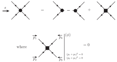
Figure 5: Rewriting the full four-quark interaction in the diquark-free-channel as an effective scalar-pseudoscalar meson exchange and a residual four-quark interaction (square), $\Gamma_{\bar{q}q\bar{q}q}^{(4),\text{{res}}_{\phi}}$ [see Equation 10]. For better accessibility we also indicate the direction of the $s$-channel.

$$\,\Gamma_{\bar{q}q\bar{q}q,k}(q,-q+p,-q^{\prime})$$

$$= \,\Gamma^{(4),{\text{{res}}}_{\phi}}_{\bar{q}q\bar{q}q,k}(q,-q+p,-q^{\prime})+\Gamma^{(4),(\phi)}_{\bar{q}q\bar{q}q,k}(q,-q+p,-q^{\prime})\,,$$ (10)

see also Figure 5. From the derivation it is evident that the scalar-pseudoscalar projection of the residual vertex vanishes on the channel with vanishing diquark momentum,

$$\left.\Gamma^{(4),{\text{{res}}}_{\phi}}_{\bar{q}q\bar{q}q,k}(q,-q+p,-q)\right|^{(\phi)}\equiv 0\,.$$ (11)

Equation 10 and Equation 11 imply in particular that the scalar-pseudoscalar part of the residual four-quark interaction vanishes at vanishing momentum, $p_{1}=p_{2}=p_{3}=p_{4}=0$. Hence the one-meson exchange captures the leading four-quark term in a derivative expansion that supposedly works at low energies. Note also that $\Gamma^{(4),\text{{res}}_{\phi}}_{\bar{q}q\bar{q}q,k}$ still has a scalar-pseudoscalar part. Firstly, the scalar-pseudoscalar $t$-channel is still present. Secondly, the full four-quark vertex carries more momentum dependence as is captured by the $t,s,u$-channels. Still, the channel where the diquark momentum vanishes is the dominant momentum structure, which suggests the above reparametrisation. The identity Equation 10 with Equation 6 and Equation 11 is depicted in Figure 5. We emphasise that the above formulation avoids any double-counting problem present in effective field theories and the effective mesonic field is merely a book-keeping device for potentially resonant channels in scattering vertices.

Equation 10 defines a reparametrisation of the effective action; on the level of momentum-independent approximations for vertices and classical dispersions for all fields involved (also the effective ones) this leads us to an effective action that also involves the mesonic fields. This reparametrisation can be performed at all scales $k$, thus removing the scalar and pseudoscalar diquark channel in the four-quark interaction. This $k$-dependent procedure can be systematically implemented, (see [22, 24, 25]), and is called dynamical hadronisation in the context of QCD. It has been developed further in [27, 26]. Here we extend it explicitly to diquarks and baryons in Secs. IV.4 and V.2.

Carrying out this procedure for the $\sigma$-$\vec{\pi}$ channel leads to an effective Lagrangian with constituent quarks and light mesons as effective degrees of freedom. For the sake of simplicity we consider only momentum-independent couplings and classical dispersions. For $N_{f}=2$ this leads us to

$$\Gamma^{\rm(qm)}_{k} =\int_{x}\biggl{\{}Z_{q}\,\bar{q}(\not{D}-\mu_{\text{q}}\gamma^{0})q+\frac{Z_{\phi}}{2}\,\partial_{\mu}\phi_{i}\partial^{\mu}\phi_{i}$$

$$\quad-\frac{\lambda_{q\phi}}{2}\,Z_{q}^{2}\Bigl{[}(\bar{q}q)^{2}+(\bar{q}i\gamma^{5}\vec{\tau}q)^{2}\Bigr{]}$$

$$\quad+\frac{h_{q\phi}}{2}\,Z_{q}Z_{\phi}^{1/2}\,\bar{q}(\sigma+i\gamma^{5}\vec{\tau}\cdot\vec{\pi})q+U_{k}(\phi)\biggr{\}}\,.$$ (12)

The first line comprises the kinetic terms of the quarks and the effective meson fields, where $Z_{q},Z_{\phi}$ are the wave-function renormalisations of quarks and mesons, respectively. The Dirac operator $\not{D}(A)$ indicates a potentially non-trivial background gauge field at finite temperature. In the current approximation they only carry a scale-dependence which is not explicitly shown in Equation 12 for notational simplicity. This also allows us to identify $\mu_{\text{q}}$ with the RG-invariant quark chemical potential. The second line is the scalar-pseudoscalar four-quark interaction that is generated from the QCD flow in the chiral limit. We have also pulled out the appropriate $Z_{q}^{2}$-factor such that the four-quark coupling $\lambda_{q\phi}$ is RG-invariant but cutoff scale-dependent. The last line carries the one-meson exchange interaction with the Yukawa coupling $h_{q\phi}$. As for the four-quark coupling it is RG-invariant. Finally we allow for a mesonic effective potential, which describes multi-meson self-interactions. In a purely fermionic language this relates to higher-order fermionic scatterings: $\phi^{(2n)}$ interaction terms relate to fermionic scatterings up to $(\bar{q}q)^{2n}$. Its precise form will be discussed later. Here we simply note that it includes mass terms for the mesons as

$$U_{k}({\phi^{2}}/{2})=\frac{1}{2}Z_{\phi}m_{\phi}^{2}\phi^{2}+O\left((\phi^{2})^{2}\right)\,.$$ (13)

In the regime with chiral symmetry breaking the expectation value of the meson field is $\phi_{\text{\tiny{EoM}}}^{2}=\sigma_{\text{\tiny{EoM}}}^{2}\neq 0$. Then we have different masses, wave-function renormalisations, etc., for $\sigma$ and $\vec{\pi}$.

The form Equation 12 can be reduced with the help of dynamical hadronisation. As described above, it allows us to rewrite certain momentum channels partially or completely in terms of effective mesonic interactions. Residual four-quark interactions in other channels have to be kept in principle.

At this point we would like to stress the necessity of including a wave-function renormalisation factor $Z_{\phi}$ corresponding to the composite mesonic operator to distribute the original four-quark coupling properly onto mass and Yukawa coupling. For the approximation Equation 12, Equation 6 reduces to

$$\lambda_{q\phi}(p^{2})=\frac{1}{2}\frac{h_{q\phi}^{2}}{p^{2}+m_{\phi}^{2}}\,.$$ (14)

Equation 14 is one of the basic equations in the present set-up and we discuss it here in some detail: Let us also remark that in the full theory both sides will be field-dependent. For example, if we only consider a constant mesonic background $\phi$, we arrive at

$$\lambda_{q\phi}(\phi,p^{2})=\frac{1}{2}\sum_{\phi_{i}=\sigma,\vec{\pi}}\frac{\left(h_{q\phi}(\phi)+h_{q\phi\phi_{i}}^{(1)}(\phi)\phi_{i}\right)^{2}}{p^{2}+m_{\phi}^{2}(\phi)}\,,$$ (15)

and $h_{q\phi\phi_{i}}^{(1)}=\partial_{\phi_{i}}h_{q\phi}$. The field-dependence of the Yukawa couplings encodes multi-meson–$q\bar{q}$ scattering processes in the scalar-pseudoscalar channel. Equation 15 is relevant for an evaluation on the equations of motion of the mesons, $\phi_{\text{\tiny{EoM}}}=(\sigma_{\text{\tiny{EoM}}},\vec{0})$ with a vanishing $\vec{\pi}$ expectation value and a non-vanishing $\sigma$ one. Then, the derivative term vanishes for the $\vec{\pi}$-directions and gives contributions in the $\sigma$-direction. Note also that the constituent quark mass is $M_{\text{q}}=\frac{1}{2}h_{q\phi}\,\sigma$, and hence is proportional to $\Gamma^{(3)}_{q\bar{q}\vec{\pi}}(\phi=(\sigma,\vec{0}))$ while $\Gamma^{(3)}_{q\bar{q}\sigma}(\phi=(\sigma,\vec{0}))$ is proportional to $h_{q\phi}(\sigma)+h_{q\phi\sigma}^{(1)}(\sigma)\,\sigma$. Moreover, seemingly the constituent quark mass $M_{\text{q}}=\frac{1}{2}h_{q\phi}\sigma$ vanishes for $\sigma\to 0$. However, it has been shown in [129] that in the full theory the Yukawa coupling $h_{q\phi}(\sigma)$ has a non-trivial $\sigma$-dependence leading to $M_{\text{q}}(\sigma)\geq M_{\text{q}}(\sigma_{\text{\tiny{EoM}}})$ for all $\sigma$.

Moreover, seemingly Equation 14 does not depend on $Z_{\phi}$; however, the flow of the coefficient of the mass term, $Z_{\phi}m_{\phi}^{2}$, is that of $\Gamma_{\phi\phi,k}^{(2)}(p=0)$. Then the flow of the mass $m_{\phi}^{2}$ is obtained from

$$\partial_{t}m^{2}_{\phi}=\partial_{t}\Gamma_{\phi\phi,k}^{(2)}(p=0)+\eta_{\phi}m^{2}_{\phi}\,,\quad\eta_{\phi}=-\frac{\partial_{t}Z_{\phi}}{Z_{\phi}}\,.$$ (16)

If we work within the approximation $Z_{\phi}=1$, the term proportional to $\eta_{\phi}$ disappears. However, the diagrammatic flow $\partial_{t}\Gamma_{\phi\phi,k}^{(2)}$ is that of $Z_{\phi}m_{\phi}^{2}$, and still carries the running of $Z_{\phi}$. Only by subtracting the $\eta_{\phi}$-term do we project on the RG-invariant flow of $m_{\phi}$, and we are led to an interesting observation: by definition $m_{\phi}$ is the Euclidean curvature mass (for a detailed discussion of the pole, screening, and curvature masses, see [130]). There it has been shown that indeed the curvature and pole masses of the pion are very close in fully-momentum dependent approximations in [130], with the discrepancy of curvature and pole masses being on the percent level. This is related to the fact that the pion pole is the first pole in the complex plane and the momentum dependence of the pion wave-function renormalisation is weak in the Euclidean domain.

In the present approximation with scale-dependent, but momentum-independent, wave-function renormalisation $Z_{\phi}$, the pole mass of the pion equals the curvature mass on the level of the effective action. Moreover, due to the weak momentum dependence its value is already close (percent level) to the one computed within fully momentum-dependent approximations, see [130]. For the reduced approximation with $\eta_{\phi}=0$ the latter property does not hold. While pole and curvature masses still agree on the level of the effective action, their values are off by roughly 30%.

IV.3.2 Emergent diquarks

We now consider an equivalent procedure for diquarks. It is evident from the discussion so far, that the effective exchange fields do not need to be colourless as they only represent exchange channels in a given four-quark scattering vertex. Hence, the introduction of these composite fields does not imply their existence as asymptotic states. Following our discussions on diquarks we are particularly interested in four-quark interactions corresponding to a scalar diquark channel. For $N_{f}=2$ this is a colour triplet and flavour singlet channel. A simple form is given by the Lagrangian,

$$\mathcal{L}_{(\bar{q}q)^{2}}^{(d)}=-\frac{1}{2}Z_{q}^{2}\lambda_{qd}(q^{T}\epsilon^{a}\tau^{2}C\gamma^{5}q)(\bar{q}\epsilon^{a}\tau^{2}C\gamma^{5}\bar{q}^{T})\,,$$ (17)

where $C=\gamma^{2}\gamma^{0}$ denotes the charge conjugation matrix, $\{\epsilon^{a}\}_{bc}=\epsilon^{abc}$ and $\tau^{2}$ the second Pauli matrix in flavour space. Note that the related tensor structure $T^{(1)}_{\rm d}$ mixes with the scalar-pseudoscalar one, $T_{\rm s}$, derived from Section IV.3.1 in the current Fierz basis in Appendix A. While this is not a conceptual problem, and it may be even advisable to keep Equation 17 for explicit computations, some of the following equations and discussions are more complicated in the presence of a mixing. Orthogonality can be achieved by one of the following procedures: we either build-up an orthogonal Fierz basis with the first two basis elements, $T_{\rm s}$ and $T^{(1)}_{\rm d}$. A further possibility for enforcing orthogonality of the scalar-pseudoscalar tensor structure and the diquark one is to stick to the Fierz basis in Appendix A and project $T^{(1)}_{\rm d}$ on the complement of $T_{\rm s}$ such that

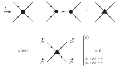
Figure 6: Rewriting the residual momentum-dependent four-quark interaction in the $s=0$ channel in Equation 10 (square) as an effective diquark exchange in the diquark tensor structure Equation 17 and a further residual four-quark interaction (triangle). For better accessibility we also indicates the direction of the $t$-channel.

$$T_{\rm d}^{(2)}=(1-P_{\rm s})T^{(1)}_{\rm d}(1-P_{\rm s})\,,$$ (18)

where $P_{\rm s}$ is the projection on the scalar-pseudoscalar subspace with $P_{\rm s}T_{\rm s}=T_{\rm s}P_{\rm s}=T_{\rm s}$ and $T_{\rm s}(1-P_{\rm s})=0$. The corresponding Lagrangian is now simply

$$\mathcal{L}_{(\bar{q}q)^{2}}^{(d)}=-\frac{\lambda_{qd}}{2}Z_{q}^{2}\,\bar{q}^{\bar{\bm{a}}_{1}}q^{\bm{a}_{1}}\bar{q}^{\bar{\bm{a}}_{2}}q^{\bm{a}_{2}}\,T_{\rm d}^{(2),\bar{\bm{a}}_{1}\bm{a}_{1}\bar{\bm{a}}_{2}\bm{a}_{2}}\,.$$ (19)

For the rest of our formal analysis both procedures are equivalent, and we shall refer to both possibilities as $T_{\rm d}$. Hence we proceed analogously to Equation 6 and subtract an effective scalar diquark exchange e.g. in a channel where $s=0$ from the residual four-quark vertex defined in Equation 10. This channel is given by $p_{2}=-p_{1}=q$ and $p_{4}=-p_{3}=p-q$. The scalar-pseudoscalar meson exchange does not contribute as the two tensor structures are orthogonal in the chosen Fierz-complete basis. The one-diquark–exchange equation reads

$$\Gamma^{(4),{\text{res}}_{\phi}}_{\bar{q}q\bar{q}q,k}(-q^{\prime},q,q^{\prime}-p)=\Gamma^{(4),{\text{{res}}}_{\phi d}}_{\bar{q}q\bar{q}q,k}(-q^{\prime},q,q^{\prime}-p)$$

$$\quad+\Gamma^{(3)}_{qqd,k}(q,p-q,p)G_{d,k}(p)\Gamma^{(3)}_{\bar{q}\bar{q}d^{*},k}(q^{\prime},p-q^{\prime},p)\,,$$ (20)

with

$$\left.\Gamma^{(4),\text{{res}}_{\phi d}}_{\bar{q}q\bar{q}q,k}(-q,q,q-p)\right|^{(d)}\equiv 0\,.$$ (21)

For the pictorial representation, see Figure 6. As for the meson exchange the above relation can be embedded in an effective action $\Gamma_{\text{\tiny QCD},k}^{(\phi d)}$ which agrees with $\Gamma_{\text{\tiny QCD},k}$ on the equations of motion for $\phi$ and $d$,

$$\Gamma_{\text{\tiny{QCD}},k}[A,c,\bar{c},q,\bar{q}]=\Gamma_{\text{\tiny{QCD}},k}^{(\phi d)}[A,c,\bar{c},q,\bar{q},\phi_{\text{\tiny{EoM}}},d_{\text{\tiny{EoM}}}]\,.$$ (22)

Then, Equation 20 includes further higher order terms, as already discussed below Equation 4. This will be fully resolved within dynamical hadronisation in Section IV.4. Note also that the orthogonal projection with $T_{\rm d}$ and $T_{\rm s}$ is already paid off: if the two tensor structures would have an overlap the two bosonisations as described here would not commute, and the results would depend on the order. In turn, with the present orthogonal tensor structures the two bosonisations commute and the order is irrelevant.

The corresponding terms of the effective action leading to Equation 12, Equation 20, and Equation 21 read for $T_{\rm d}^{(1)}$,

$$\Gamma^{\rm(qd)}_{k}= \,\int d^{4}x\biggl{\{}Z_{d}(D_{\mu}-\mu_{\text{d}}\delta_{\mu 0})d^{a}(D^{\mu}+\mu_{\text{d}}\delta^{\mu 0})d^{a\ast}$$

$$\hskip 22.76228pt-\frac{\lambda_{qd}}{2}\,Z_{q}^{2}\,\left(q^{T}\epsilon^{a}\tau^{2}C\gamma^{5}q\right)\left(\bar{q}\epsilon^{a}\tau^{2}C\gamma^{5}\bar{q}^{T}\right)$$

$$+\frac{h_{qd}}{2\sqrt{2}}\,Z_{q}Z_{d}^{\frac{1}{2}}\left[d^{a\ast}\!\left(q^{T}\!\epsilon^{a}\tau^{2}C\gamma^{5}q\right)\!+\!d^{a}\!\left(\bar{q}\epsilon^{a}\tau^{2}C\gamma^{5}\bar{q}^{T}\right)\!\right]\!\biggr{\}},$$ (23)

where $d^{a}$ denotes the complex scalar diquark field with the diquark chemical potential given by $\mu_{\text{d}}=2\mu_{\text{q}}$. As for the quark-meson action we have pulled out the appropriate powers of the wave-function renormalisations $Z_{q},Z_{d}$ for having RG-invariant running couplings $\lambda_{qd},h_{qd}$. The action defined in Equation 23 does not contain an explicit mass term for the diquark. Instead, in Equation 12, we include an effective potential of the form,

$$U_{k}=U^{\rm(md)}_{k}(\rho_{\rm\phi},\rho_{\rm d})\,,$$ (24)

as a function of two invariants,

$$\rho_{\rm\phi}\mathrel{\mathop{\mathchar 58\relax}}=\frac{1}{2}\sum_{i}\phi_{i}^{2}\,,\qquad\rho_{\rm d}\mathrel{\mathop{\mathchar 58\relax}}=\sum_{a}d^{a\ast}d^{a}\,.$$ (25)

Linear terms in $\rho_{\rm\phi}$ and $\rho_{\rm d}$ in the potential give rise to mass terms $m_{\phi}^{2}\rho_{\rm\phi}$ and $m_{d}^{2}\rho_{\rm d}$ in the symmetric phase for mesons and diquarks, respectively. Higher order terms are interpreted as inter-meson, inter-diquark, and meson-diquark interactions arising from mixed terms in the potential. The corresponding action for $T_{\rm d}^{(2)}$ is just obtained by the projection in Equation 18. Again we emphasise that the difference is not the projection but rather the different Fierz bases.

IV.3.3 Emergent vector mesons

In the same line as above we can introduce an effective field $\phi_{\mu}$ for vector mesons

$$\phi_{\mu}=\omega_{\mu}+V_{\mu}\,,\quad V_{\mu}=\rho_{\mu}^{a}\tau^{a}+a_{1\mu}^{a}\tau_{5}^{a}\,,$$ (26)

where $\tfrac{1}{2}(\tau^{a}\pm\tau_{5}^{a})$ are the generators of $SU(2)_{R/L}$ respectively. The vector field $\phi_{\mu}$ has the entries $(\phi_{\mu}^{i})=(\omega_{\mu},\vec{\rho}_{\mu},\vec{a_{1}}_{\mu})$. In the present context the field $V_{\mu}=(\rho_{\mu},a_{1\mu})$ is added for the sake of completeness and for later applications beyond the scope of the present paper. The four-quark tensor structure corresponding to the $\omega_{\mu}$ is derived straightforwardly from the Fierz basis in Appendix A: it is given by the symmetric combination of $\mathcal{L}^{(V-A)}_{(\bar{q}q)^{2}}+\mathcal{L}^{(V+A)}_{(\bar{q}q)^{2}}$ in Equation 89, and we dropped the axial-vector tensor structure $\mathcal{L}^{(V-A)}_{(\bar{q}q)^{2}}-\mathcal{L}^{(V+A)}_{(\bar{q}q)^{2}}$. In turn, the $\rho,a_{1}$-tensor structures are more complicated in terms of the basis Equation 89, and we refrain from showing them explicitly.

The different components of the vector field $\phi_{\mu}$ are relevant for an appropriate description of the onset of nuclear matter via $\omega$, as well as the access to $\rho$-physics via $V_{\mu}$. The latter has been treated within dynamical hadronisation in [28]. The quark-vector meson part of the action reads in analogy to Equation 12, Equation 23,

$$\Gamma^{\rm(qV)}_{k}=\int_{x}\Biggl{\{}\frac{Z_{\omega}}{4}\,(\partial_{\mu}\omega_{\nu}-\partial_{\nu}\omega_{\mu})^{2}+\frac{Z_{V}}{4}\,(\partial_{\mu}V^{i}_{\nu}-\partial_{\nu}V^{i}_{\mu})^{2}$$

$$\quad-\frac{\lambda_{q\omega}}{2}\,Z_{q}^{2}\left(\bar{q}\gamma^{\mu}q\right)^{2}-\frac{\lambda_{qV}}{4}\,Z_{q}^{2}\Bigl{[}\left(\bar{q}\gamma^{\mu}\vec{\tau}q\right)^{2}+(\bar{q}\gamma^{\mu}\gamma^{5}\vec{\tau}q)^{2}\Bigr{]}$$

$$\quad+\frac{h_{q\omega}}{2}\,\ Z_{q}Z_{\omega}^{1/2}\,\bar{q}\gamma^{\mu}\omega^{\mu}q$$

$$\quad+\frac{h_{qV}}{2}\,\ Z_{q}Z_{V}^{1/2}\,\bar{q}\left(\gamma^{\mu}\vec{\tau}\cdot\vec{\rho}^{\mu}+\gamma^{\mu}\gamma^{5}\vec{\tau}\cdot\vec{a}_{1}^{\mu}\right)q\Biggr{\}}\,,$$ (27)

where the potential $U_{k}$ in Equation 12 now also depends on the vector mesons $\phi_{\mu}$, i.e., $U_{k}=U_{k}(\phi,\phi_{\mu},d)$. Most notably, in the regime with vector meson dominance (VMD) we have

$$\frac{1}{4}(\partial_{\mu}V^{i}_{\nu}-\partial_{\nu}V^{i}_{\mu})^{2}+U_{k}(\phi,V_{\mu},d)=\frac{1}{2}\text{tr}\,F_{\mu\nu}(V_{\mu})^{2}+\cdots$$ (28)

with the non-Abelian field strength $F_{\mu\nu}(V_{\mu})$. In the present dynamical hadronisation approach to first principle QCD, vector meson dominance is not assumed. It is or is not the outcome of the dynamical computation, for a first work in this direction, see [28].

IV.4 Dynamical hadronisation for mesons and diquarks

Dynamical hadronisation has been invented under the name of rebosonisation for bilinear composite operators in [22]. In [24] it has been extended to general composite operators, for further work see [25]. In the present work we build on the formulation [26, 27, 29, 10] for QCD that also takes into account the full momentum dependence of vertices.

IV.4.1 Dynamical hadronisation for scalar-pseudoscalar mesons

Let us first describe the essential idea behind dynamical hadronisation at the standard QCD example of the light scalar-pseudoscalar mesons $\phi=(\sigma,\vec{\pi})$ along the discussion in [26, 27, 29, 10]: first we note that the fields $\sigma,\vec{\pi}$ have the quantum numbers of $\bar{q}q\,,\,\bar{q}i\gamma_{5}\vec{\tau}q$ states. The simplest identification would be $\phi\propto D_{\bar{q}q,k}\,(\bar{q}q\,,\,\bar{q}i\gamma_{5}\vec{\tau}q)$. In the last section we have introduced $\phi$ as an effective field for a one-meson exchange that describes the related resonant scalar-pseudoscalar channel with vanishing diquark momentum in the full four-quark scattering vertex $\Gamma^{(4)}_{\bar{q}q\bar{q}q}$, see Equation 9. It is clear from the discussion there, that the prefactor $D_{\bar{q}q,k}$ is related to the interaction strength of the related four-quark interaction. Moreover, a rescaling as indicated in Equation 8 also changes the normalisation of the fields with $\phi\to{D}_{\phi}\phi$. This leads to the notion of a $k$-dependent change of the composite field $\phi_{k}$, which we parametrise as

$$\partial_{t}\begin{pmatrix}\sigma_{k}\\ \vec{\pi}_{k}\end{pmatrix}\!(r)=\dot{D}_{\bar{q}q}(r)\frac{Z_{q}}{Z_{\phi}^{\frac{1}{2}}}\!\begin{pmatrix}\bar{q}q\\ \bar{q}i\gamma^{5}\vec{\tau}q\end{pmatrix}\!(r)+\dot{D}_{\phi}(r)\!\begin{pmatrix}\sigma_{k}\\ \vec{\pi}_{k}\end{pmatrix}\!(r)\,,$$ (29)

where $(\bar{q}q)(r)=\int_{l}\bar{q}(l)q(r-l)$, and $(\bar{q}i\gamma^{5}\vec{\tau}q)(r)$ is defined similarly. The field $(Z_{q}/Z_{\phi}^{1/2})(\bar{q}q\,,\,\bar{q}i\gamma^{5}\vec{\tau}q)$ has the same RG-running as the mesonic field, and hence the coefficients of the dynamical hadronisation, $\dot{D}_{\bar{q}q},\dot{D}_{\phi}$, are RG-invariant. Equation 29 is the reduction of the fully general dynamical hadronisation with local operators in the $t=0$ channel with $\dot{D}_{\bar{q}q}(l,r-l)$ to the plain $u$-channel discussed in [27]. The general case will be considered elsewhere. The coefficients $\dot{D}_{\bar{q}q}=\partial_{t}D_{\bar{q}q}$ and $\dot{D}_{\phi}=\partial_{t}D_{\phi}$ may have a matrix structure in the chiral broken phase where the degeneracy with respect to $\sigma_{k}$ and $\vec{\pi}_{k}$ is lost. As the flow equation for the effective action was derived for $k$-independent fields, the left hand side of the flow equation now changes to

$$\partial_{t}\Gamma_{\text{\tiny{QCD}},k}\to\partial_{t}\Gamma_{\text{\tiny{QCD}},k}^{(\phi)}[\Phi]+\int_{x}\partial_{t}\Phi_{i,k}[\Phi]\frac{\delta\Gamma_{\text{\tiny{QCD}},k}^{(\phi)}[\Phi]}{\delta\Phi_{i}}\,,$$ (30)

where the $t$-derivatives are always taken at fixed fields. This already explains the dynamical hadronisation term on the left hand side of Equation 1. We also emphasise that the argument of the effective action, the mean field $\Phi$, is $t$-independent.

Let us discuss the related modification of the flows at the example of the full mesonic two-point function,

$$\Gamma^{(2)}_{\phi,k}(p)=Z_{\phi}(p)\left(p^{2}+m^{2}_{\phi}\right)\,,$$ (31)

with a momentum-dependent wave-function renormalisation $Z_{\phi}(p)$ and a momentum-independent, but cutoff scale-dependent mass $m_{\phi}^{2}$. Note that the parametrisation in Equation 31 is not unique, we may even absorb the mass $m_{\phi}^{2}$ completely in the wave function renormalisation: $Z_{\phi}\to Z_{\phi}\,p^{2}/(p^{2}+m_{\phi}^{2})$. The rescaling property of $D_{\phi,k}$ becomes evident from the form of the flow equation for the mesonic two-point function at vanishing fields,

$$\frac{1}{\Gamma^{(2)}_{\phi,k}(p)}\left(\partial_{t}+2\dot{D}_{\phi}(p)\right)\Gamma^{(2)}_{\phi,k}(p)$$

$$=\left(2\dot{D}_{\phi}(p)-\eta_{\phi}(p)\right)+\frac{\partial_{t}m_{\phi}^{2}}{p^{2}+m_{\phi}^{2}}=\frac{1}{\Gamma^{(2)}_{\phi,k}(p)}{\rm Flow}^{(2)}_{\phi}(p)\,,$$ (32)

with the anomalous dimension

$$\eta_{\phi}(p)=-\frac{\partial_{t}Z_{\phi}(p)}{Z_{\phi}(p)}\,.$$ (33)

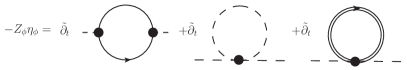
Figure 7: Schematic representation of the flow equation for the bosonic anomalous dimension in the symmetric phase (permutations, signs, and diagram multiplicities are not shown).

The left hand side of Equation 32 is obtained straightforwardly from taking the second $\phi$-derivative of Equation 30 at $\Phi=0$, while the right hand side stands for the diagrams contributing to the flow of the mesonic two-point function. Evidently, the mesonic two-point function is proportional to a factor $\exp(2D_{\phi,k}(p))$ as introduced in Equation 8. The contributing terms include contributions from the quark loop proportional to $h_{q\phi}$, see Figure 7, and hence ${Z_{\phi}}_{k}\neq 0$ even with $Z_{\phi}=0$ at the initial UV scale. In turn, $-2\dot{D}_{\phi}$ accounts for the rescaling shift of the anomalous dimension. If we choose $\dot{D}_{\phi}$ such that it compensates for the $\partial_{t}m_{\phi}^{2}$ term and the diagrammatic contribution,

$$2\dot{D}_{\phi}(p)=-\frac{\partial_{t}m_{\phi}^{2}}{p^{2}+m_{\phi}^{2}}+\frac{1}{\Gamma^{(2)}_{\phi,k}(p)}{\rm Flow}^{(2)}_{\phi}(p)\,,$$ (34)

the anomalous dimension vanishes identically for all cutoff scales, $\eta_{\phi}(p)\equiv 0$. This is in line with the rescaling symmetry in Equation 8 which can be used to shift the dependence on the exchange momentum between the Yukawa vertex and the meson propagator.

For the sake of simplicity, the discussion above was done in the case of vanishing backgrounds in the symmetric phase. If expanding the flows about non-vanishing backgrounds, i.e., in the regime with chiral symmetry breaking, the equations receive further straightforward contributions.

For the determination of $\dot{D}_{\bar{q}q}$, see later discussions in Section IV.4.4.

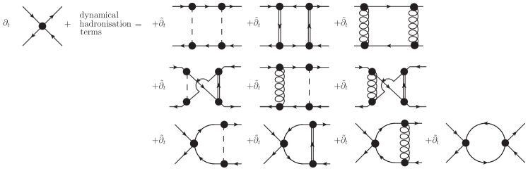
Figure 8: Schematic representation of the flow equation for the four-quark coupling with dynamical hadronisation of the scalar-pseudoscalar and the scalar diquark channel (permutations, signs, and diagram multiplicities are not shown).

IV.4.2 Dynamical hadronisation for diquarks

In summary, the above introduction of composite meson fields allows for partial and full bosonisations of the respective four-quark interaction channels with a specific choice of the dispersion of the composite fields. It is the constraint equations for $\dot{D}_{\bar{q}q},\dot{D}_{\phi}$ which settles the related choice. Before we discuss these constraints, we extend the above argument to the diquark sector. In analogy to Equation 29 we write,

$$\partial_{t}\begin{pmatrix}d^{a}_{k}\\ d^{a\ast}_{k}\end{pmatrix}=\dot{D}_{qq}\frac{Z_{q}}{Z_{d}^{\frac{1}{2}}}\sqrt{2}\begin{pmatrix}q^{T}\epsilon^{a}\tau^{2}C\gamma^{5}q\\ \bar{q}\epsilon^{a}\tau^{2}C\gamma^{5}\bar{q}^{T}\end{pmatrix}+\dot{D}_{d}\begin{pmatrix}d^{a}_{k}\\ d^{a\ast}_{k}\end{pmatrix}\,.$$ (35)

Equation 29 and Equation 35 encode the mixing effect of the four-quark interaction and the Yukawa interaction during the fRG-flow. They can be used to impose that the respective residual channels of the four-quark interaction vanish, see Equation 11 and Equation 21. This is complete bosonisation of the respective channels, and it entails in particular that the respective four-quark couplings vanish for all scales $k$ at vanishing momenta, $\lambda_{q\phi}=\lambda_{qd}=0$. Due to the consistent book keeping during the flow any double counting problem is avoided.

IV.4.3 Dynamical hadronisation for vector mesons

The dynamical hadronisation flows that comes with the quark-vector meson action Equation 27 read

$$\partial_{t}\omega_{k}^{\mu}(r)=\dot{D}_{\bar{q}\gamma q}(r)\frac{Z_{q}}{Z_{\omega}^{\frac{1}{2}}}(\bar{q}\gamma^{\mu}q)(r)+\dot{D}_{\omega}(r)\,\omega_{k}^{\mu}(r)\,,$$ (36)

and

$$\partial_{t}\begin{pmatrix}\vec{\rho}_{k}^{\mu}\\ \vec{a}_{1k}^{\mu}\end{pmatrix}(r)$$

$$=\dot{D}_{\bar{q}\gamma\tau q}(r)\frac{Z_{q}}{Z_{V}^{\frac{1}{2}}}\begin{pmatrix}\bar{q}\gamma^{\mu}\vec{\tau}q\\ \bar{q}\gamma^{\mu}\gamma^{5}\vec{\tau}q\end{pmatrix}(r)+\dot{D}_{V}(r)\,\begin{pmatrix}\vec{\rho}_{k}^{\mu}\\ \vec{a}_{1k}^{\mu}\end{pmatrix}(r)\,.$$ (37)

IV.4.4 Complete dynamical hadronisation

Let us now elaborate on the case of a complete dynamical hadronisation, concentrating on the scalar-pseudoscalar and the vector channel first, i.e., on the $\lambda_{q\phi/d}=0$ constraints. The flow equations for $\lambda_{q\phi/d}$ is obtained by taking for quark–anti-quark derivatives of the flow Equation 1. These four derivatives also hit the rebosonisation term on the right hand side of Equation 30, and generate $\dot{D}_{qq}h_{q\phi}$ and $\dot{D}_{d}h_{qd}$ terms, respectively. Then the four-quark flows can be derived from Equation 1 including the dynamical hadronisation terms similarly to the flow of the mesonic two-point function Equation 32. For the sake of simplicity we restrict ourselves to the vanishing momentum part and vanishing backgrounds $\Phi=0$ in the symmetric phase, to wit

$$\partial_{t}\lambda_{q\phi}-2\eta_{q}\,\lambda_{q\phi}-2h_{q\phi}\dot{D}_{\bar{q}q}= \,\frac{1}{Z_{q}^{2}}{\rm Flow}^{(4)}_{\phi,qq\bar{q}\bar{q}}\,,$$

$$\partial_{t}\lambda_{qd}-2\eta_{q}\,\lambda_{qd}-2h_{qd}\dot{D}_{qq}= \,\frac{1}{Z_{q}^{2}}{\rm Flow}^{(4)}_{\text{d},qq\bar{q}\bar{q}}\,,$$ (38)

where ${\rm Flow}^{(4)}_{\phi/\rm d}$ stands for the diagrammatic contributions coming from the right hand side of Equation 1, see Figure 8.

For large cutoff scales the four-quark couplings vanish, and in particular we have $\lim_{k\to\infty}\lambda_{q\phi/d}\to 0$. If we adjust the dynamical hadronisation functions $\dot{D}_{\phi/d}$ such, that the flows $\left(\partial_{t}-2\eta_{q}\right)\lambda_{q\phi/d}\equiv 0$, these couplings vanish identically also for vanishing cutoff scale $k=0$. This is obtained by imposing

$$\dot{D}_{\bar{q}q}=-\frac{1}{Z_{q}^{2}}\frac{{\rm Flow}^{(4)}_{\phi,qq\bar{q}\bar{q}}}{2h_{q\phi}}\,,\qquad\dot{D}_{qq}=-\frac{1}{Z_{q}^{2}}\frac{{\rm Flow}^{(4)}_{\text{d},qq\bar{q}\bar{q}}}{2h_{qd}}\,,$$ (39)

where the right hand sides are RG-invariant by construction. This leads us to

$$\lambda_{q\phi}\equiv 0\,,\qquad\qquad\lambda_{qd}\equiv 0\,.$$ (40)

In conclusion we have shown how to eliminate momentum channels of specific tensor structure of the four-quark interaction with the choice of the dynamical hadronisation functions $\dot{D}_{\bar{q}q/qq}$. Furthermore, the scaling functions $\dot{D}_{\phi/d}$ can be used to re parametrise the meson and diquark propagators, or, more generally, the meson and diquark fields in a momentum-dependent way. This may help to optimise the physics content of expansion schemes where only part of the full momentum dependence is taken into account.

Subject to an appropriate diagonalisation of the Fierz basis the vector meson channel of the four-quark interaction can be eliminated with the condition,

$$\dot{D}_{\bar{q}\gamma q}=-\frac{1}{Z_{q}^{2}}\frac{{\rm Flow}^{(4)}_{\omega,qq\bar{q}\bar{q}}}{2h_{q\omega}}\,,\quad\dot{D}_{\bar{q}\gamma\tau q}=-\frac{1}{Z_{q}^{2}}\frac{{\rm Flow}^{(4)}_{\text{V},qq\bar{q}\bar{q}}}{2h_{qV}}\,,$$ (41)

where we have restricted ourselves to $\Phi=0$ in the symmetric phase as for the mesons and diquarks. For later purposes we already mention, that for $\omega$ in the broken phase, apart from terms proportional to $\Gamma^{(5)}_{\omega qq\bar{q}\bar{q}}$, the denominator in Equation 41 is changed to $h_{q\omega}+h^{(1)}_{q\omega\omega_{0}}\,\omega_{0}$ similarly to the scalar-pseudoscalar meson case.

Equation 41 together with Equation 39 leads to complete dynamical hadronisation of the scalar-pseudoscalar and vector meson channels as well as the scalar diquark channel of the four-quark interaction. The effective potential $U_{k}(\phi,\phi_{\mu},d)$ then carries multi-meson-diquark scatterings in these channels. The link to the effective action of QCD in terms of the fundamental degrees of freedom $\Phi_{\text{\tiny{fund}}}=(A,c,\bar{c},q,\bar{q})$ is now given by

$$\Gamma_{\text{\tiny{QCD}},k}[\Phi_{\text{\tiny{fund}}}]=\Gamma_{\text{\tiny{QCD}},k}^{(\phi\phi_{\mu}d)}[\Phi_{\text{\tiny{fund}}},\phi_{\text{\tiny{EoM}}},\phi_{\mu,\text{\tiny{EoM}}},d_{\text{\tiny{EoM}}}]\,.$$ (42)

In the present context we are most interested in the $\omega_{0}$-part of the vector meson action. It couples to higher correlation functions of the quark, and in particular to the baryon channel of the six-quark interaction. There, it provides a density field for the baryon density in addition to the chemical potential. A non-vanishing expectation value of $\omega_{0}$ hence shifts the onset of the baryon density and influences the liquid-gas transition. We shall come back to this point at the end of the next section on emergent baryons.

For later reference we present at this point in more detail the four-quark interaction channels relevant in this work, namely the four-quark couplings corresponding to the scalar-pseudoscalar channel $\lambda_{q\phi}$, the scalar diquark channel $\lambda_{qd}$ and the vector $\lambda_{q\omega}$, evaluated on the solution presented in Ref. [27]. In terms of the Fierz-complete basis from App. A these are given by

$$\lambda_{q\phi} =\lambda_{(S-P)_{+}}+\lambda_{(S+P)_{-}}\,,$$

$$\lambda_{qd} =\frac{2}{3}\lambda_{q\phi}-\frac{2}{3}\lambda_{(S-P)_{-}}+\frac{2}{3}\lambda_{(S+P)_{-}}+\frac{2}{3}\lambda_{(V-A)}\,,$$

$$\quad-2\lambda_{(S+P)_{-}^{\rm adj}}-2\lambda_{(V-A)^{\rm adj}}\,,$$

$$\lambda_{q\omega} =\lambda_{(V-A)}+\lambda_{(V+A)}\,.$$ (43)

It turns out that the scalar diquark channel is attractive, see [27, 29], consistent with weak-coupling arguments [131, 132, 133].

V Emergent Baryons

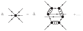
Figure 9: UV-flow of six-quark interactions via quark-gluon ring diagrams.

Having discussed the four-quark interactions along with its reformulation in terms of effective mesonic/diquark degrees of freedom in details, we now turn to six-quark interactions. For this discussion we start from the QCD framework, where the scalar-pseudoscalar channel, and the scalar diquark channel have been treated within dynamical hadronisation. Here we consider the baryon channel of the six-quark interaction.

V.1 Qualitative features of baryon flows

At large scales, analogously to the generation of the four-quark interaction, the six-quark interaction is generated and sustained by the quark-gluon ring diagrams, see Figure 9. This diagram runs with $\alpha_{s,k}^{3}$. All other diagrams in terms of quarks and gluons are suppressed with additional powers of $\alpha_{s,k}$, and hence will be neglected in the current UV analysis.

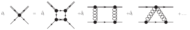
Figure 10: UV-flow of two-quark–two-diquark interactions via quark-diquark box, quark-diquark-gluon box, and quark-gluon triangle diagrams.

Due to the introduction of the effective diquark field $d\propto qq$ the UV-flow also generates diquark-quark box diagrams that have the same effective quark content as the quark-gluon ring, see Figure 10. A comparison of their relative strength in terms of the running coupling is only possible after the equations of motion for $\phi,d$ are invoked. Without this the hadron correlation functions have the scaling symmetry Equation 8 or, in the dynamical hadronisation context, the choice of $\dot{D}_{\phi/d}$ in Equation 29 and Equation 35. Only combinations of hadron correlation functions that are symmetric under these rescalings may relate directly to diagrams in QCD without dynamical hadronisation.

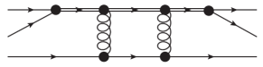
Figure 11: Relevance counting for two-quark–two-diquark interactions compared to six-quark interactions for the example of the quark-diquark-gluon box diagram.

If the equations of motion, $\phi_{\text{\tiny{EoM}}},d_{\text{\tiny{EoM}}}$ are invoked, external meson and diquark lines receive at leading order a further scattering in $\bar{q}q$ and $qq$, respectively, via the Yukawa interaction, see, e.g., Figure 11 for the quark-diquark-gluon box. The upper line in Figure 11 now describes the scattering of two quarks into a diquark, the subsequent emission of two gluons and then the rescattering of the diquark into two quarks. We also observe that the lower part of the quark-gluon box and the triangle diagram are the same. The upper line of the combination of these diagrams follows from two gluon field derivatives of a diquark propagator, i.e.,

$$\left.\frac{\delta^{2}}{\delta A^{2}}\right|_{h_{qd}}h_{qd}G_{\rm d}h_{qd}= \,-h_{qd}G_{\rm d}\Gamma_{dd^{*}AA}^{(4)}G_{\rm d}h_{qd}$$

$$+h_{qd}G_{\rm d}\Gamma_{dd^{*}A}^{(3)}G_{\rm d}\Gamma_{dd^{*}A}^{(3)}G_{\rm d}h_{qd}\,.$$ (44)

Now we utilise that the tree-level diagram of the quark-diquark (re-)scattering $h_{qd}G_{\rm d}h_{qd}$ scales as $\alpha_{s,k}^{2}$ in the UV as it relates to the four-quark vertex that is driven by the gluonic box diagram, see Figure 2 and Figure 6. In summary this leads to an $\alpha_{s,k}^{4}$-scaling for both the triangle diagram and the quark-diquark-gluon box.

The $\alpha_{s,k}$ scaling of the quark-diquark box follows similarly: attaching the diquark-quark scattering arising from the equations of motion the diagram is constructed solely from

$$\left(h_{qd}G_{\rm d}h_{qd}\right)^{3}\propto\alpha_{s,k}^{6}\,.$$ (45)

Using the fact that $h_{qd}G_{\rm d}h_{qd}$ scales as $\alpha_{s}^{2}$ in the UV finally leads to an overall $\alpha_{s,k}$-scaling of $\alpha_{s}^{6}$. We conclude that in the UV the diquark diagrams are suppressed by at least one additional power of $\alpha_{s,k}$ compared to the quark-gluon ring diagram in Figure 11 that scales as $\alpha_{s,k}^{3}$.

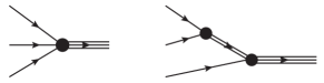
Figure 12: Competing baryon creation processes: direct process involving three quarks (left) and 2-step process involving an intermediate diquark.

While the diquark diagrams are suppressed in the UV, we expect them to be relevant in the IR due to phase space arguments, see Figure 12. A related analysis will be published elsewhere. The baryon channels of the six-quark interaction, as well as the two-quark–two-diquark interaction are defined by the tensor structure as well as the baryon momentum routing.

At this point it is instructive to consider three quark interpolation operators for baryons and their chiral transformation properties. The most obvious choice involving a scalar diquark structure is

$$(q^{T}\epsilon^{a}\tau^{2}C\gamma^{5}q)q^{a}\,,$$ (46)

or correspondingly

$$\sqrt{2}d^{a}q^{a}\,,$$ (47)

which transforms as a quark under axial chiral $SU(2)_{A}$ transformations as the diquark operator is a chiral scalar [63, 64]. Note that we completely disregard the transformation properties with respect to axial $U(1)_{A}$ transformations that linearly mixes interpolating operators with scalar and pseudoscalar diquark structure, see App. B. We now consider six-quark interaction terms that are generated in the effective action corresponding to a classical Lagrangian of the form,

$$\mathcal{L}_{(6q)}=\lambda_{qb}Z_{q}^{3}(\bar{q}\epsilon^{a}\tau^{2}C\gamma^{5}\bar{q}^{T})(q^{T}\epsilon^{b}\tau^{2}C\gamma^{5}q)(\bar{q}^{a}\mathcal{T}q^{b})\,,$$ (48)

with a so far undetermined operator $\mathcal{T}$ acting in Dirac and flavour space. The simplest and most widely used choice $\mathcal{T}=\mathbbm{1}$ is obviously not invariant under $SU(2)_{A}$ transformations. One way of enforcing an $SU(2)_{A}$-invariant interaction is to consider momentum-dependent interactions with $\mathcal{T}=p^{\mu}\gamma^{\mu}$ for an appropriate momentum variable $p$.

The interaction in Equation 48 is now treated with dynamical hadronisation analogously to the mesons and diquarks. In terms of the Bethe-Salpether language used to heuristically describe the hadronisation of mesons and diquarks we rewrite the baryon channels in terms of a one-baryon exchange, see Figure 13.

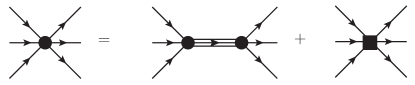
Figure 13: Rewriting the six-quark interaction as an effective baryon exchange and a residual six-quark interaction (square).

To that end we have to define the baryon propagator. In the chiral limit at $\sigma=0$ the propagator $G_{\rm b}$ of the exchange effective field $b$ has to sustain the chiral structure of the interaction. Accordingly we write

$$G_{\rm b}(p)=\frac{1}{Z_{b}(p)}\frac{1}{i\not{p}}\,,$$ (49)

in the UV. The quark-gluon triangle, the diquark-quark-gluon box and the diquark-quark box diagrams in the baryon channel generate a two-quark–two-diquark interaction in the effective action. The classical Lagrangian corresponding to Equation 48 on the quark-diquark level reads

$$\mathcal{L}_{(2q2d)}=\lambda_{qdb}\,Z_{q}Z_{d}\,d^{\ast}_{a}d^{\phantom{\ast}}_{b}(\bar{q}_{a}\mathcal{T}q_{b})\,.$$ (50)

Analogous to the six-quark interaction we can rewrite the two-quark–two-diquark interaction as an effective baryon exchange and a residual interaction, see Figure 14. It is important to keep in mind that, although six-quark interaction and the two-diquark share the same effective quark content, they have to be considered for the sake of the baryonisation as two independent interactions.

In summary, the baryonic effective action that gives rise to the one-baryon exchange diagrams in Figure 13 and 14 on the equation of motion of the baryon reads

$$\Gamma^{\rm(b)}_{k}=\int d^{4}x\,\biggl{\{}Z_{b}\bar{b}\left(\not{\partial}-\mu_{\text{b}}\gamma^{0}\right)b$$

$$+2\lambda_{qdb}\,Z_{q}Z_{d}\,d^{\ast}_{a}d^{\phantom{\ast}}_{b}\left(\bar{q}_{a}\mathcal{T}q_{b}\right)$$

$$+\lambda_{qb}\,Z_{q}^{3}\,\left(\bar{q}\epsilon^{a}\tau^{2}C\gamma^{5}\bar{q}^{T}\right)\left(q^{T}\epsilon^{b}\tau^{2}C\gamma^{5}q\right)\left(\bar{q}_{a}\mathcal{T}q_{b}\right)$$

$$+\sqrt{2}h_{qdb}\,Z_{q}^{1/2}Z_{d}^{1/2}Z_{b}^{1/2}\,\left[d^{\phantom{\ast}}_{a}\left(\bar{b}\mathcal{T}q_{a}\right)+d_{a}^{\ast}\left(\bar{q}_{a}\mathcal{T}b\right)\right]$$

$$+h_{qb}\,Z_{q}^{3}Z_{b}^{1/2}\,\left[\left(q^{T}\epsilon^{a}\tau^{2}C\gamma^{5}q\right)\left(\bar{b}\mathcal{T}q_{a}\right)+{\rm h.c.}\right]\biggr{\}}\,.$$ (51)

As for the meson and diquark effective action we have pulled out the appropriate factors of the wave-function renormalisations in order to have RG-invariant couplings. The second and the third lines contain the terms generated from quark-gluon-meson-diquark interactions in QCD formulated with dynamical hadronisation of mesons and diquarks with the effective action $\Gamma^{(\phi\phi_{\mu}d)}_{\text{\tiny{QCD}},k}$, see Equation 42. The fourth and the fifth lines provide the Yukawa terms that describe the scattering of a quark and a diquark into the effective baryon field and that of three quarks into the effective baryon field.

We also emphasise that no explicit baryon term is present. In the chiral limit in the UV, no mass term is present for $\sigma=0$. In turn, for $\sigma\neq 0$ the six-quark exchange diagram leads to non-chiral structures in the baryon channel that lead to mass terms in the dispersion Equation 49. In the effective action Equation 51 this is encoded in the meson-baryon terms in the last line. In the IR, where spontaneous chiral symmetry breaking occurs, the expectation value of the $\sigma$-field takes a non-trivial value and the baryon curvature mass in the IR reads

$$M_{\text{b}}(\sigma)=\frac{1}{2}h_{b\phi}\sigma\qquad{\rm and}\qquad M_{\text{b}}=\frac{1}{2}h_{b\phi}\sigma_{\text{\tiny EoM}}\,,$$ (52)

analogously to the quark mass. Note that in both cases the structure $M(\sigma)=\frac{1}{2}h\,\sigma$ seems to imply that the mass function vanishes for $\sigma=0$ even in the chirally broken phase. However, it has been shown in [129] that in the full theory the Yukawa coupling $h(\sigma)$ has a non-trivial $\sigma$-dependence leading to $M(\sigma)\geq M(\sigma_{\text{\tiny{EoM}}})$ for all $\sigma$. In any case, the baryon propagator is given by

$$G_{\rm b}(p)=\frac{1}{Z_{b}(p)}\frac{1}{i\not{p}+M_{\text{b}}(\sigma)}\,.$$ (53)

This structure immediately leads to the question how the chiral baryon decouples in the UV. Typically this decoupling, as in the case of mesons and diquarks, is achieved by a rapidly increasing mass. The decoupling of the baryon is guaranteed by the equivalence of a baryon exchange with the Yukawa-type interaction with $h_{qb},h_{qdb}$ to the respective six-quark and two-quark–two-diquark interactions. Relying on the approximation Equation 51 they read very schematically,

$$Z_{q}^{3}h_{qb}\mathcal{T}\frac{1}{\not{p}}\mathcal{T}h_{qb}\,,\qquad\qquad Z_{q}Z_{d}h_{qdb}\mathcal{T}\frac{1}{\not{p}}\mathcal{T}h_{qdb}\,.$$ (54)

Note that $Z_{b}$ from the propagator is cancelled by the respective $Z_{b}$ in the interaction terms. The wave-function renormalisations of quarks and diquarks in Equation 54 take care of the natural scalings of quarks and diquarks. Accordingly, the normalised, RG-invariant Yukawa couplings $h_{qb},h_{qdb}$ have to vanish in the UV. In summary, the mass-decoupling for meson and diquark turns into a vertex-decoupling for the baryon. The link to QCD in the fundamental degrees of freedom is now given by

$$\Gamma_{\text{\tiny{QCD}},k}[\Phi_{\text{\tiny{fund}}}]=\Gamma_{\text{\tiny{QCD}},k}^{(\phi\phi_{\mu}d)}[\Phi_{\text{\tiny{fund}}},\phi_{\text{\tiny{EoM}}},\phi_{\mu,\text{\tiny{EoM}}},d_{\text{\tiny{EoM}}},b=0]\,,$$ (55)

as the fermionic baryon field $b$ has to vanish on the equations of motion, $b_{\text{\tiny{EoM}}}=0$.

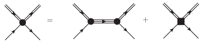
Figure 14: Rewriting the two-quark–two-diquark interaction as an effective baryon exchange and a residual two-quark–two-diquark interaction (square).

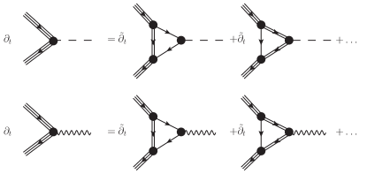
Figure 15: Creation of effective baryon-meson (first line: scalar/pseudoscalar; second line: vector) interaction via a quark-diquark loop diagram.

The Ansatz for the effective action in Equation 51 are all sixth order in effective quark degrees of freedom. There are of course higher order terms that are generated during the flow, such as eight-point interactions in effective quark degrees of freedom, or in terms of baryonic interactions, baryon-meson and baryon-quark interaction terms. This is reflected by an Ansatz for the effective action of the form,

$$\Gamma^{\rm(bm)}_{k}=\int d^{4}x\biggl{[}\frac{h_{b\phi}}{2}Z_{\phi}^{1/2}Z_{b}\,\bar{b}\,(\sigma+i\gamma^{5}\vec{\pi}\cdot\vec{\tau})b$$

$$+\frac{h_{\omega\rm b}}{2}Z_{\omega}^{1/2}Z_{b}\,\bar{b}\,\gamma_{\mu}\omega_{\mu}b-\lambda_{b\omega}Z_{b}Z_{q}(\bar{b}\gamma_{\mu}b)\,(\bar{q}\gamma_{\mu}q)\biggl{]}\,,$$ (56)

where we have dropped terms coupling the baryon to the vector mesons $V_{\mu}$. The Ansatz Equation 56 takes into account the emission and absorption of mesons, $\phi,\phi_{\mu}$ from/into a baryon, see Figure 15. Note that the $\omega_{0}$-contribution can be absorbed in a shift of the chemical potential: $\mu\to\mu-h_{q\omega}Z_{\omega}\omega_{0}$. For later reference Equation 56 also includes a quark-baryon scattering term. Even in an approximation scheme with momentum-independent dressing functions, it is not guaranteed that the complete dynamical hadronisation of the vector channel $\lambda_{q\omega}$ also leads to a complete dynamical hadronisation of the two-quark-two-baryon interaction in the eighth order in effective quark degrees of freedom. The omission of this interaction introduces an artificial dependence on the choice of the basis in the sector of four-quark interactions.

V.2 Dynamical hadronisation for baryons

So far we have discussed the qualitative features of the hadronisation for baryons. In the present section we put forward the dynamical hadronisation procedure for baryons. The $k$-dependent change of the baryon field that allows to remove the effective baryon-exchange contribution from the six-quark as well as two-quark–two-diquark channels is given by

$$\partial_{t}\begin{pmatrix}b_{k}\\ \bar{b}_{k}\end{pmatrix}=\dot{D}_{qqq}\,\frac{Z_{q}^{3/2}}{Z_{b}^{1/2}}\begin{pmatrix}(q^{T}\epsilon^{a}\tau^{2}C\gamma^{5}q)q^{a}\\ \bar{q}^{a}(\bar{q}\epsilon^{a}\tau^{2}C\gamma^{5}\bar{q}^{T})\end{pmatrix}$$

$$\qquad+\dot{D}_{qd}\,\frac{Z_{q}^{1/2}Z_{d}^{1/2}}{Z_{b}^{1/2}}\sqrt{2}\begin{pmatrix}d_{k}^{a}q^{a}\\ d_{k}^{a}{}^{*}\bar{q}^{a}\end{pmatrix}+\dot{D}_{b}\begin{pmatrix}b_{k}\\ \bar{b}_{k}\end{pmatrix}\,,$$ (57)

where we build on the identification in Equation 46 and Equation 47. Note that there is no mixing between $\dot{D}_{qqq}$ and $\dot{D}_{qd}$ on the level of these equation as the former relates to six-quark and the latter to two-quark–two-diquark flows. As for mesons and diquarks we restrict ourselves to the vanishing momentum part for the sake of simplicity. By projecting the full flows for the six-point and two-quark–two-diquark correlation functions on the baryon tensor structures, see Figure 9 and 10, we arrive at

$$\partial_{t}\lambda_{qb}-3\eta_{\rm q}\lambda_{qb}+2h_{qb}\dot{D}_{qqq}= \,\frac{1}{Z_{q}^{3}}{\rm Flow}^{(6)}_{\rm q}\,,$$

$$\partial_{t}\lambda_{qdb}-(\eta_{\rm q}+\eta_{\rm d})\lambda_{qdb}+2h_{qdb}\dot{D}_{qd}= \,\frac{1}{Z_{q}Z_{d}}{\rm Flow}^{(4)}_{\rm qd}\,,$$ (58)

where ${\rm Flow}^{(6)}_{\rm q}$ and ${\rm Flow}^{(4)}_{\rm qd}$ stand for the corresponding diagrammatic contributions coming from the right hand side of Equation 1. For large cutoff scales the six-quark and two-quark–two-diquark couplings vanish, and in particular we have $\lim_{k\to\infty}\lambda_{qb}\to 0$ and $\lim_{k\to\infty}\lambda_{qdb}\to 0$. If we adjust the dynamical hadronisation functions $\dot{D}_{qqq/qd}$ such that both flows vanish, i.e., $\partial_{t}\lambda_{qb}\equiv\partial_{t}\lambda_{qdb}\equiv 0$, these couplings vanish identically also for vanishing cutoff scale $k=0$. This is obtained by imposing

$$\dot{D}_{qqq}= \,\frac{1}{2h_{qb}}\frac{1}{Z_{q}^{3}}{\rm Flow}^{(6)}_{\rm q}\,,$$

$$\dot{D}_{qd}= \,\frac{1}{2h_{qdb}}\frac{1}{Z_{q}Z_{d}}{\rm Flow}^{(4)}_{\rm qd}\,,$$ (59)

where the right hand sides are RG-invariant by construction. This leads us to

$$\lambda_{qb}\equiv 0\,,\qquad\qquad\lambda_{qdb}\equiv 0\,.$$ (60)

In conclusion we have shown how to eliminate momentum channels of specific tensor structures of the six-quark interaction with the choice of the dynamical hadronisation functions $\dot{D}_{qqq/qd}$. Furthermore, the scaling function $\dot{D}_{b}$ can be used to reparametrise the baryon propagator. However, as can be seen from the equations, it has dropped out completely in the normalised, RG-invariant representation as it should.

Finally, we discuss how the baryonic mass scale arises diagrammatically from Figure 9: the baryonic mass scale is that of the pole mass. For that purpose we have to Wick-rotate the Euclidean imaginary time frequencies $\omega_{\textrm{Eucl}}$ to Minkowski real time frequencies $\omega_{\textrm{Min}}$,

$$\omega_{\textrm{Eucl}}=\text{i}\,\omega_{\textrm{Min}}\,.$$ (61)

Due to the relation between the baryonic propagator and the quark-gluon ring as well as the quark-diquark box diagrams, a resonance in the latter corresponds to a pole in the former or a resonance in the quark-diquark-baryon coupling $h_{qdb}$ and the quark-baryon coupling $\lambda_{qqqb}$. This relation also extends to the flow of the diagrams.

Let us now discuss the structure in detail. To begin with, we first consider a one loop approximation with momentum and cutoff independent dressings of vertices and propagators. Then resonances in the diagrams occur at the frequency $\omega_{\text{\tiny Min}}=3m_{{\rm q},\text{\tiny con}}$ with a constituent mass $m_{{\rm q},\text{\tiny con}}=m_{\rm q}/Z_{q}$ as well as $\omega_{\text{\tiny Min}}=m_{{\rm q},\text{\tiny con}}+m_{{\rm d},\text{\tiny con}}$ with $m_{{\rm d},\text{\tiny con}}=m_{\rm d}/Z_{d}$.

Within the next, already non-trivial approximation we consider cutoff-dependent vertices, wave-function renormalisations and mass functions. Then the pole mass, or more precisely the first cut or pole in the complex plane, is obtained from integrating the flow. Seemingly it is then given by the relations above for the constant dressing at vanishing cutoff scale. However, the flows of the dressings are not necessarily monotonous. This feature is indicative for a non-monotonous momentum-dependence of the baryonic diagrams. Accordingly the cut or pole may be at a lower frequency as that obtained with the dressings at vanishing cutoff. This entails that the physical baryon mass $m_{\rm b}/Z_{b}$ has an upper bound by $3m_{{\rm q},\text{\tiny con}}$ as well as $m_{q,\text{\tiny con}}+m_{{\rm d},\text{\tiny con}}$. These bounds are close to each other due to the small flow effects in the diquark sector.

Furthermore, the large mass scales in the diagrams support a derivative expansion in the baryonic diagrams. For that reason the above Minkowski argument transports straightforwardly to Euclidean space and the flows of $m_{\rm b}$ and $Z_{b}$ reflect the above properties. In summary we deduce that the baryon mass, up to a small binding energy derived from the flow, has to agree with $3m_{{\rm q},\text{\tiny con}}$ apart from small differences between $m_{{\rm d},\text{\tiny con}}$ and $2m_{{\rm q},\text{\tiny con}}$. These considerations are also important for the discussion of the onset of the baryonic density at the liquid-gas transition.

V.3 Towards basic properties of baryonic matter

The set-up with dynamical hadronisation enables us to encompass in a unified approach to both vacuum QCD and the regime with the nuclear liquid-gas transition. In the present section we discuss this set-up, and in particular its foundation in the Silver Blaze property of QCD [134]. The latter property, roughly speaking, entails that at vanishing temperature below the onset of baryon density at an onset chemical potential $\mu_{q,\textrm{onset}}$ no observable depends on the chemical potential. Here, $\mu_{q,\textrm{onset}}$ equals the excitation energy of the lowest lying state in QCD. More formally speaking, it signals the distance of the lowest lying pole or cut in the complex plane for correlation functions that carry baryon charge.

This approach aims at a first principle access to the baryonic onset density and the binding energy of nuclear matter from dynamically hadronised vector mesons, the results of which will be discussed elsewhere. We begin with a short review of the Silver Blaze property in QCD in the context of the fRG approach [66, 135, 136]. In particular in [66] it has been shown from the fRG that at vanishing temperature and $\mu_{q}\leq\mu_{q,\textrm{onset}}$ all $q,\bar{q}$ correlation functions in QCD satisfy the following Silver Blaze property,

$$\Gamma^{(n)}_{q_{1}\cdots q_{n}\bar{q}_{n+1}\cdots\bar{q}_{2n}}(\omega_{1},...,\omega_{2n};\mu_{q})$$

$$= \,\Gamma^{(n)}_{q_{1}\cdots q_{n}\bar{q}_{n+1}\cdots\bar{q}_{2n}}(\omega_{1}+i\mu_{q},...,\omega_{2n}-i\mu_{q};0)\,.$$ (62)

In Equation 62 we have restricted ourselves to quark–anti-quark correlation functions, the extension to general QCD correlation functions is straightforward. Moreover, we suppressed the dependence on spatial momenta, which are irrelevant for our present discussions. Equation 62 simply entails the fact that below onset the frequency integration $q_{0}$ in the flow can be shifted with $q_{0}+i\mu_{q}\to q_{0}$ in order to absorb the chemical potential. With Equation 62 the $\mu_{q}$-independence of observables follows trivially. For example, the chiral condensate $\Delta_{q}$ satisfies at $T=0$,

$$\Delta_{q}(\mu_{q})\propto \,\int_{{\rm l}\!{\rm R}}\frac{dq_{0}}{2\pi}\text{tr}\,G_{\bar{q}q}(q_{0};\mu_{q})$$

$$= \,\int_{{\rm l}\!{\rm R}}\frac{dq_{0}}{2\pi}\text{tr}\,G_{\bar{q}q}(q_{0}+i\mu_{q};0)=\Delta_{q}(0)\,.$$ (63)

In the last step in Equation 63 we used that the loop integration can be shifted with $q_{0}+i\mu_{q}\to q_{0}$ for $\mu_{q}<\mu_{q,\textrm{onset}}$. Note also that in Equation 63 we concentrated on the Silver Blaze property and hence the frequency integration while dropping the spatial momentum integrals which require renormalisation. For practical purposes it is far more convenient to consider the flow of the condensate, for more details see e.g. [10].

The seemingly trivial property Equation 63 has indeed far reaching consequences. In the formalism developed here we have already explained how vector mesons emerge and $\omega_{0}$ particularly has the same quantum number as the density. Because $\omega_{0}$ and the density share the same quantum number, $\omega_{0}$ should acquire a non-zero background at finite density. Assuming a simultaneous complete hadronisation on the level of four-quark as well as eight-quark interactions, we can most efficiently carry out the resummation with respect to the background by introducing shifted chemical potentials via

$$\bar{\mu}_{\rm q/d/b}=\mu_{\rm q/d/b}-\frac{1}{2}h_{\omega\rm q/d/b}\;\bar{\omega}\,,$$ (64)

with the normalised RG-invariant field $\bar{\omega}=Z_{\omega}^{1/2}\omega_{0}$ and where we for notational simplicity denoted the $\omega d^{*}d-$coupling in the effective potential by $h_{\omega\rm d}$. Indeed, the interactions between the $\omega_{0}$-meson and the baryon and diquark originate in triangle diagrams with a quark-$\omega_{0}$ Yukawa interaction. Note that the shift in the chemical potential is momentum-dependent; strictly speaking, Equation 64 reads

$$\bar{\mu}_{\rm q/d/b}(q,p-q)=\mu_{\rm q/d/b}\,\delta(p)-\frac{1}{2}h_{\omega\rm q/d/b}(q,p-q)\bar{\omega}(p),$$ (65)

where $p$ is the $\omega_{0}$ momentum, $q$ is the quark momenta and $p-q$ is that of the anti-quark. For example, Equation 65 leads to $\int_{r,s}\bar{q}(r-s)\gamma_{0}\bar{\mu}_{\rm q}(s,r)q(s)$ in the effective action action.

For a first investigation we restrict ourselves to a constant $h_{\omega\rm q/d/b}\,\bar{\omega}$ and a field-independent $\omega_{0}$-mass $m_{\omega}^{2}$. Then, Equation 65 reduces to Equation 64, which simply constitutes a shift in the chemical potential. Then, the whole $\omega_{0}$-dependence beyond the kinetic term is that in $\bar{\mu}_{\rm q/d/b}$. This allows us to invoke the Silver Blaze property for correlation functions, Equation 62, which now reads

$$\Gamma^{(n)}_{q_{1}\cdots q_{n}\bar{q}_{n+1}\cdots\bar{q}_{2n}}(p_{1},...,p_{2n};\mu_{q},\omega_{0})$$

$$=\Gamma^{(n)}_{q_{1}\cdots q_{n}\bar{q}_{n+1}\cdots\bar{q}_{2n}}(\bar{p}_{1},...,\bar{p}_{2n};0,0)\,,$$ (66)

where we have defined $\bar{p}=(\bar{p}_{0},\vec{p})$ with

$$\bar{p}_{0}\equiv p_{0}+i\,\alpha_{\rm q/d/b}\left(\mu_{\text{q}}-\frac{1}{2}h_{\omega\rm q}\,\bar{\omega}\right)\,.$$ (67)

In Equation 67, $\alpha_{\Phi_{i}}$ for $\Phi_{i}=\rm q,d,b$ is defined to match the baryon number of $\Phi_{i}$ given by $\alpha_{\Phi_{i}}/3$. This leads us to the surprising property that the part of the effective potential $V_{\omega}(\bar{\omega})$ of the $\omega_{0}$-meson only consists out of the mass term induced by dynamical hadronisation,

$$V_{\omega}(\bar{\omega})=\frac{1}{2}m_{\omega}^{2}\bar{\omega}^{2}\,.$$ (68)

Despite the approximation of constant $h_{\omega\rm q/d/b}\,\bar{\omega}$ and a field-independent $\omega_{0}$-mass this is a very strong constraint on the dynamics of the vector-channel. Now we consider the general case as follows.

Firstly, we emphasise that the present analysis does not entail the absence of momentum-dependent interactions of the $\omega$-meson with momentum $p$. These interactions are present, but are suppressed in the low energy limit for $p\to 0$.

Secondly, the $\omega$-mass depends on the scalar–pseudoscalar mesons $\phi=(\sigma,\vec{\pi})$ via the field-dependent quark masses $m_{q}(\phi)$. Consequently, even for constant fields Equation 68 is an approximation, but interactions are only triggered by scalar-pseudoscalar loops. In the ultraviolet the $\phi$-dynamics is strongly suppressed, while in the infrared the $\omega_{0}-\phi$ interaction is suppressed by powers of the constituent quark mass. In summary this amounts to Equation 68 being a very good approximation of the full potential.

We now apply the analysis above to the full system of flow equations. These equations are built upon the propagators, and in particular on diquark and baryon propagators. With Silver Blaze, Equation 66, all propagators are functions of the shifted frequency Equation 67 below the baryonic onset, to wit

$$G_{\Phi_{i}}(p_{0},\vec{p};\mu_{\Phi_{i}},\bar{\omega})=G_{\Phi_{i}}(\bar{p}_{0},\vec{p};0,0)\,.$$ (69)

Hence the Yukawa couplings follow from that of the quark to $\omega_{0}$ as

$$h_{\omega\rm d}=2h_{\omega\rm q}\,,\qquad h_{\omega\rm b}=3h_{\omega\rm q}\,,$$ (70)

and with Equation 64 we obtain

$$\bar{\mu}_{\text{d}}=2\bar{\mu}_{\text{q}}\,,\qquad\bar{\mu}_{\text{b}}=3\bar{\mu}_{\text{q}}\,,$$ (71)

below the baryonic onset. As already discussed above, strictly speaking, this relation only holds for constant shifts of the chemical potential, but we shall apply this to the full Yukawa couplings. However, even for momentum-dependent Yukawa couplings the relations Equation 67 and Equation 70 will remain valid up to the point where a pole prevents a shift of the integration contour. As we will see, the main region of interest is at small momenta, where this is not expected to be an issue.

Now we come back to the effective potential $V_{\omega}$. We have derived from the Silver Blaze property, that, in a good approximation, the potential only includes the mass term of the $\omega_{0}$ meson, see Equation 68. Evidently, the potential should be symmetric in $\omega_{0}^{2}+\vec{\omega}^{2}$ due to $O(4)$-symmetry, also not allowing for interacting $\vec{\omega}$-terms. To see this, we extend our discussion concerning $\omega_{0}$ to the spatial components $\vec{\omega}$. Indeed, the same Silver Blaze type argument we have used for $\omega_{0}$ also applies to the $\vec{\omega}$-mesons, and we illustrate this at the example of the coupling to the quark: the $\vec{\omega}$ effectively shift the spatial momentum $\vec{q}$ to $\vec{q}-\tfrac{i}{2}h_{\omega\rm q}\vec{\omega}$, and hence below the threshold of the quark the correlation functions are simply $\vec{\omega}$-independent functions of the shifted momentum argument. Including also the frequency relation Equation 67 we are led to the observation that in a general $\bar{\omega}_{\mu}$-background below the onset the propagators will only depend on

$$\bar{p}_{\mu}\mathrel{\mathop{\mathchar 58\relax}}=p_{\mu}+i\,\alpha_{\rm q/d/b}\left(\mu_{\text{q}}\delta_{0\mu}-\frac{1}{2}h_{\omega\rm q}\,\bar{\omega}_{\mu}\right)\,,$$ (72)

generalising Equation 67 and hence Equation 69. We emphasise that this entails that the effective potential below onset does not receive $\omega$-dependent contributions from charged particle, i.e., quark, diquark or baryon loops. This is an essential difference compared to the $\sigma$-dependent contributions to the potential. Note however, that a Taylor expansion in $\omega_{0}$ or $\mu$ about $\omega=0$ and $\bar{\mu}$ below onset provides non-vanishing coefficients due to the non-analyticity of the Silver Blaze property: for example, expanding in $\mu$ or $\omega_{0}$ relates to an expansion in $A_{0}$ at vanishing momentum, the Taylor coefficients of the power $2n$ are identical up to $(-)^{n}$, the odd ones vanish.

In summary, the grand potential,

$$\Omega[\Phi;\bar{\mu})=\frac{T}{\cal V}\Gamma[\Phi]\,,$$ (73)

with the spatial volume $\cal V$ at vanishing pion field, $\vec{\pi}=0$, has the following unique decomposition,

$$\Omega(\sigma,\bar{\omega},\bar{\mu})=\Omega_{\phi}(\sigma)+\Omega_{\bar{\omega}}(\bar{\omega})+\Delta\Omega_{\bar{\mu}}(\sigma,\bar{\omega},\bar{\mu})\,,$$ (74)

where $\bar{\mu}$ stands for momentum-dependent $\bar{\mu}_{\text{q}},\bar{\mu}_{\text{d}},\bar{\mu}_{\text{b}}$ in Equation 65 and the last term in Equation 74 stands for the density-contributions,

$$\Delta\Omega_{\bar{\mu}}(\sigma,\bar{\omega},\bar{\mu})=\Omega(\sigma,\bar{\omega},\bar{\mu})-\Omega(\sigma,\bar{\omega},0)\,.$$ (75)

In turn, the first two terms are simply the grand potential at vanishing chemical potential and density,

$$\Omega(\sigma,\bar{\omega},0)=\Omega_{\phi}(\sigma)+\Omega_{\bar{\omega}}(\bar{\omega})\,.$$ (76)

The first term originates from the quark-gluon and scalar-pseudoscalar loops in the flow equation. The second part is generated directly by the dynamical hadronisation of the vector meson channel. As we have already discussed before, for constant fields and Yukawa couplings and field-independent quark mass terms, the effective potential of the $\omega$-meson is only given by the mass term below onset chemical potential, see Equation 68. In this regime, both the momentum-dependent interactions as well as that triggered by the exchange of $\sigma$’s and $\vec{\pi}$’s can be considered to be small and we conclude

$$\Omega_{\bar{\omega}}(\bar{\omega})\approx\frac{1}{2}m^{2}_{\bar{\omega}}\,\bar{\omega}^{2}\,,$$ (77)

where $m_{\bar{\omega}}$ is the curvature mass of the $\omega$-meson. This entails that the full $\omega$-dependence on the action is carried by a free action $\Gamma_{\bar{\omega}}[\bar{\omega}]$ with a general dispersion,

$$\Gamma_{\bar{\omega}}[\bar{\omega}]=\frac{1}{2}\int_{p}Z_{\omega}(p^{2})\,\omega(p)\,\left[p^{2}+m^{2}_{\omega}(p^{2})\right]\,\omega(-p)\,.$$ (78)

The dispersion is fully determined by the vector four-quark coupling $\lambda_{q\omega}(p)$ with

$$\lambda_{q\omega}(0,p)=\frac{1}{2}h_{\omega\rm q}(0,p)G_{\omega}(p)h_{\omega\rm q}(0,-p)\,,$$ (79)

with $\lambda_{q\omega}(0,p)=\lambda(0,p,0,-p)$ and

$$G_{\omega}(p)=\frac{1}{Z_{\omega}(p^{2})}\frac{1}{p^{2}+m^{2}_{\omega}(p^{2})}\,.$$ (80)

Here we obtained Equation 79 by evaluating the analogue of Equation 6 in the vector channel,

$$\lambda_{q\omega}(q,-q+p,-q)$$

$$=\frac{1}{2}h_{\omega\rm q}(q,p-q)G_{\omega}(p)h_{\omega\rm q}(-q,q-p)\,,$$ (81)

for vanishing quark momentum $q=0$. Note, however, that an immediate consequence of the above Silver Blaze discussion is, that also the four-fermi couplings depend on the frequencies $\bar{p}_{0}$. Accordingly, Equation 81 has the dependence

$$\lambda_{q\omega}(\bar{q},-\bar{q}+p,-\bar{q})$$

$$=\frac{1}{2}h_{\omega\rm q}(\bar{q},p-\bar{q})G_{\omega}(p)h_{\omega\rm q}(-\bar{q},\bar{q}-p)\,.$$ (82)

In conclusion the results of this section allow for a simple and quantitative access to the physics of the liquid-gas transition in QCD within functional first principles approaches: this access rests on the triviality of the $\bar{\omega}$-potential enforced by the Silver Blaze property, and the access to the frequency dependence of the four-quark interaction in the $\omega$ channel. Accordingly it only requires the quantitative computation of vacuum correlation functions of QCD as done in [27, 29].

VI Quark-hadron mixing

As soon as the mass threshold of diquarks is exceeded, they form a condensate. Inevitably, this causes a mixing effect of the energy dispersion relations of quarks and baryons. Also, a diquark condensate would induce a further mixing effect between mesons and diquarks. We can see such a mixing pattern very transparently in the flow equation for the full effective potential $U_{k}(\rho_{\rm\phi},\rho_{\rm d})$. Its flow at low energies is generated from the sum of the quark-loop, the baryon-loop, and the meson-diquark-loop,

$$\partial_{t}U_{k}=\partial_{t}U^{\rm(q)}_{k}+\partial_{t}U^{\rm(b)}_{k}+\partial_{t}U^{\rm(m\text{-}d)}_{k}\,.$$ (83)

For the sake of the present argument we restrict ourselves to the flow equation of the effective potential in the local potential approximation (LPA). We present all loop contributions in Appendix C utilising the three-dimensional analogue of the LPA-optimised regulator [137]. This should facilitate own computation of interested readers.

Moreover, the phase diagram of the related quark-meson-diquark model (without nucleons) at finite temperature and density has been worked out in [65] on the basis of the LPA-flow equation for $U_{k}$ in Equation 83, and can be compared to the respective computation in [65, 66]: the results for the phase structure in the three-color quark-diquark meson model resemble that of the two-colour quark-diquark-meson model, though it shows a much smaller ’BEC-BCS–regime (in terms of $\mu_{B}$) at low temperatures. This should be attributed to the absense of the Pauli-Gursey symmetry in three-colour, physical, QCD. The latter symmetry leads to $m_{\pi}=m_{d}$ in the two-color case and the baryonic onset starts at much smaller baryon (diquark) chemical potential.

Interestingly, also the three-color phase diagram shows the phenomenon of precondensation at large densities already found and discussed in the two-colour quark-diquark model in [66]. Whether such a precondensation phase is also present in the quark-meson-diquark-nucleon model with Equation 83, is an exciting and phenomenologically relevant open question and will be discussed elsewhere.

One part of the contribution of the quark-loop is characterised by familiar energy dispersion relations,

$$\omega=\sqrt{(\varepsilon_{\text{q}}\pm\mu_{\text{q}})^{2}+2h_{qd}^{2}\rho_{\rm d}}\;,\quad\varepsilon_{\text{q}}\equiv\sqrt{k^{2}+M_{\text{q}}^{2}}\,.$$ (84)

In a phase with a vanishing diquark condensate, $\rho_{\rm d}=0$, Equation 84 reduces to the standard expressions with dynamical masses. However, there is another more intricate contribution that arises from the mixing of quarks and baryons in the presence of a diquark condensate, see Equation 102 and Equation 107. For $\rho_{\rm d}=0$, there is no mixing between quarks and baryons (except for higher-order fluctuations). Then we find two distinct dispersion relations,

$$\omega=\pm\sqrt{k^{2}+M_{\text{q}}^{2}}-\mu_{\text{q}}\;,\quad\omega=\pm\sqrt{k^{2}+M_{\rm b}^{2}}-\mu_{\text{b}}\,,$$ (85)

for quarks, anti-quarks, baryons, and anti-baryons, respectively. The mixing of these energy dispersion relations for $\rho_{\rm d}\neq 0$ provides relevant information about the phenomenology in this phase. The mixing can be deduced from Equation 105, and is depicted in Figure 16. There we show the quark and bayron masses at functions of the momentum scale $k$. At $\rho_{\rm d}=0$ and $\mu_{\text{q}}=0$, as shown in Figure 16a, this indicates $\pm 0.939\;\text{GeV}$ for baryons and $\pm 0.4\;\text{GeV}$ for quarks, which is our input.

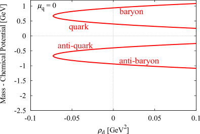
(a) $q,\bar{q},b,\bar{b}$-masses at $\mu_{\text{q}}=0\;\text{GeV}$.

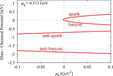
(b) $q,\bar{q},b,\bar{b}$-masses at the baryon threshold $\mu_{\text{q}}=M_{\rm b}/3=0.313\;\text{GeV}$.

Figure 16: $a,\bar{q}$ and $b,\bar{b}$ masses relative to the Fermi surface. For simplicity, $h_{qdb}$ is taken to be unity.

We notice from Figure 16a, that the quark and the baryon masses smoothly meet in a region analytically continued to $\rho_{\rm d}<0$. This link between quarks and baryons is absent in the physical $\rho_{\rm d}>0$ region. It hints at a duality of quarks and baryons, in particular when the diquarks condensate. This also suggests that the relation between the quark and baryon mass branches dictates the binding energy of baryons. Figure 16b shows the masses (relative to the quark/baryon chemical potential) at the baryon mass threshold, $\mu_{\text{q}}=M_{\rm b}/3$. We see that the baryon branch touches zero, and hence $M_{\rm b}-\mu_{\text{b}}=0$, at $\rho_{\rm d}=0$. The quark branch also approaches zero, but it remains finite because $M_{\text{q}}-\mu_{\text{q}}=0.087\;\text{GeV}>0$ there.

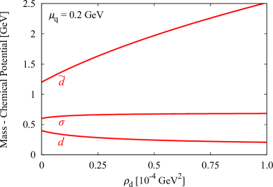
(a) $\sigma,\tilde{d},d$-masses below the diquark threshold at $\mu_{\text{q}}=0.2\;\text{GeV}$

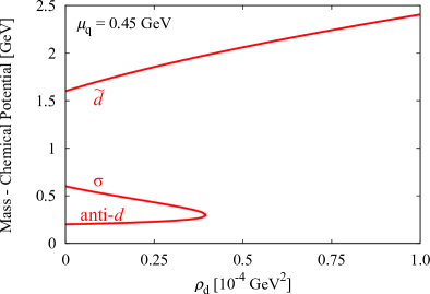
(b) $\sigma,\tilde{d},d$-masses above the diquark threshold at $\mu_{\text{q}}=0.2\;\text{GeV}$

Figure 17: Masses of $\sigma$-meson and $\tilde{d},d$-diquarks relative to the Fermi surface.

Next we discuss the meson- and the diquark-loop contributions. The respective ’physical’ bosonic degrees of freedom are the ($\pi,\sigma$)-mesons and the diquarks. However, be aware of the fact that the diquarks can have different dispersions just like the ($\pi,\sigma$) mesons, once $\rho_{\rm d}$ becomes nonzero. The $\sigma$ and pion masses are given by

$$M_{\pi}^{2}=\frac{\partial U_{k}}{\partial\rho_{\rm\phi}}\;,\qquad M_{\sigma}^{2}=\frac{\partial U_{k}}{\partial\rho_{\rm\phi}}+2\rho_{\rm\phi}\frac{\partial^{2}U_{k}}{\partial\rho_{\rm\phi}^{2}}\,.$$ (86)

Similarly, the two diquark masses read,

$$M_{d}^{2}=\frac{\partial U_{k}}{\partial\rho_{\rm d}}\,,\qquad M_{\tilde{d}}^{2}=\frac{\partial U_{k}}{\partial\rho_{\rm d}}+2\rho_{\rm d}\frac{\partial^{2}U_{k}}{\partial\rho_{\rm d}^{2}}\,,$$ (87)

and $M_{d}^{2}<M_{\tilde{d}}^{2}$.

For $\rho_{\rm\phi}\neq 0$ and $\rho_{\rm d}\neq 0$, there are also off-diagonal components in the mass matrix, that induce a mixing effect between $\sigma$ and $\tilde{d}$ (heavier diquark), see Equation 110 for an explicit expression. Then, the physical masses of $\sigma$, $\tilde{d}$, and $d$ are defined by the eigenvalues of the mass matrix.

Their mixing is quite non-trivial. In Figure 17 we have depicted an example of the behaviour of these masses as functions of the diquark condensate $\rho_{\rm d}$. For the results shown in Figure 17 we used the following lowest order Ansatz for the potential,

$$U_{k}=-m^{2}\Bigl{(}\rho_{\rm\phi}+\frac{\rho_{\rm d}}{\gamma}\Bigr{)}+g\Bigl{(}\rho_{\rm\phi}+\frac{\rho_{\rm d}}{\gamma}\Bigr{)}^{2}-h\sigma\,.$$ (88)

Equation 88, while being rather qualitative, should capture the generic properties well. We have four parameters for $U_{k}$, $\gamma$, $g$, $\rho_{\rm\phi}$, $h$, and we fix these parameters with physical observables: $\sigma=f_{\pi}=93\;\text{MeV}$, $M_{\pi}=135\;\text{MeV}$, $M_{\sigma}=600\;\text{MeV}$, $M_{\rm d}=800\;\text{MeV}$ at $\rho_{\rm d}=0$. The latter identifications of parameters with observables are the standard ones for LPA-approximations to LEFTs, the QCD-adjustments for quantitatively reliable approximations in the spirit of QCD-assisted LEFTS can be found in [27, 26, 28, 29, 10].

Then, the parameters in our model are straightforwardly determined from the relations, $h=2f_{\pi}M_{\pi}^{2}$, $\gamma=M_{\pi}^{2}/M_{d}^{2}$, $g=(M_{\sigma}^{2}-M_{\pi}^{2})/(8f_{\pi}^{2})$, and $m^{2}=M_{\sigma}^{2}/4-5M_{\pi}^{2}/4+(M_{\sigma}^{2}-M_{\pi}^{2})\rho_{\rm d}/(4f_{\pi}^{2}\gamma)$. For an analysis of the mixing pattern at finite $\rho_{\rm d}$, we simply study the $\sigma$ and $\tilde{d},d$ masses as a function of the size of the diquark condensate $\rho_{\rm d}$, while keeping all other parameters fixed.

The three lines in Figure 17a represent $M_{d}$, $M_{\sigma}$, and $M_{\tilde{d}}$ from bottom to top. The $\sigma$ mass is not directly affected by the chemical potential, so $M_{\sigma}$ at $\rho_{\rm d}=0$ stays at $0.6\;\text{GeV}$. The diquark dispersions are shifted by $2\mu_{\text{q}}=0.4\;\text{GeV}$. Accordingly, we get $M_{d}-2\mu_{\text{q}}=0.4\;\text{GeV}$ at $\rho_{\rm d}=0$. The other diquark is found to be quite massive and hence decouples from the dynamics.

With increasing $\mu_{\text{q}}$, we have smaller $M_{d}-2\mu_{\text{q}}$ and eventually a diquark condensate should develop when $M_{d}-2\mu_{\text{q}}<0$. Then, the diquark branch labelled with $d$ in Figure 17a moves below zero. At the same time, the anti-diquark branch moves up and it is connected to the $\sigma$ branch, as shown in Figure 17b for $\mu_{\text{q}}=0.45\;\text{GeV}$ which is greater than the diquark threshold.

In summary this leaves us with a very appealing, simple and coherent picture of baryonic properties at vanishing finite density. Its embedding in the first principles fRG-approach to QCD should allow for a determination of hadron masses and the physics of the liquid-gas transition at vanishing and small temperatures.

VII Conclusions

In the present work we have discussed dynamical hadronisation in QCD within the functional renormalisation group approach at the explicit example of $N_{f}=2$ flavour QCD. To date, dynamical hadronisation has mostly been applied to the light scalar-pseudoscalar $\sigma,\vec{\pi}$ mesons. The latter are introduced as effective fields for the resonant scalar-pseudoscalar channel of the four-quark correlation function. This allows us to monitor the dynamical emergence of these low energy degrees of freedom within QCD.

Here we have, for the first time, set up the dynamical hadronisation approach also for an effective diquark field $d$ for the scalar diquark channel. While the latter is not an asymptotic state it can be understood as a collective offshell degree of freedom that may become resonant at large density in the colour-superconducting phase, see e.g. [17] for an fRG study.

The final new ingredient is the extension of the dynamical hadronisation approach to baryons, i.e. the nucleons. The respective effective field takes care of both, the baryon channel in the six-quark interaction as well as the baryon channel in the two-quark–two-diquark interaction.

The approach of emergent hadrons and diquarks put forward in the present work has natural applications to the hadron resonance spectrum, the nuclear liquid-gas transition as well as the physics of nuclear and quark matter at large density.

Appendix A Four-quark interactions

We rely on the basis for $U(2)_{L}\times U(2)_{R}$ symmetric four-quark interactions already used in [27, 29], see also [139], and [34] for a review,

$$\mathcal{L}_{(\bar{q}q)^{2}}^{(S-P)_{+}^{\phantom{adj}}} =(\bar{q}T^{0}q)^{2}\!-\!(\bar{q}\gamma^{5}T^{f}q)^{2}\!-\!(\bar{q}\gamma^{5}T^{0}q)^{2}\!+\!(\bar{q}T^{f}q)^{2}\,,$$

$$\mathcal{L}_{(\bar{q}q)^{2}}^{(V-A)_{\phantom{-}}^{\phantom{adj}}} =(\bar{q}\gamma^{\mu}T^{0}q)^{2}\!+\!(\bar{q}\gamma^{\mu}\gamma^{5}T^{0}q)^{2}\,,$$

$$\mathcal{L}_{(\bar{q}q)^{2}}^{(V+A)_{\phantom{-}}^{\phantom{adj}}} =(\bar{q}\gamma^{\mu}T^{0}q)^{2}\!-\!(\bar{q}\gamma^{\mu}\gamma^{5}T^{0}q)^{2}\,,$$

$$\mathcal{L}_{(\bar{q}q)^{2}}^{(V-A)_{\phantom{-}}^{\text{adj}}} =(\bar{q}\gamma^{\mu}T^{0}T^{a}q)^{2}\!+\!(\bar{q}\gamma^{\mu}\gamma^{5}T^{0}T^{a}q)^{2}\,,$$

$$\mathcal{L}_{(\bar{q}q)^{2}}^{(S+P)_{-}^{\phantom{adj}}} =(\bar{q}T^{0}q)^{2}\!-\!(\bar{q}\gamma^{5}T^{f}q)^{2}\!+\!(\bar{q}\gamma^{5}T^{0}q)^{2}\!-\!(\bar{q}T^{f}q)^{2}\!,$$

$$\mathcal{L}_{(\bar{q}q)^{2}}^{(S+P)_{-}^{\text{adj}}} =(\bar{q}T^{0}T^{a}q)^{2}\!-\!(\bar{q}\gamma^{5}T^{f}T^{a}q)^{2}\!$$

$$\hskip 42.67912pt+\!(\bar{q}\gamma^{5}T^{0}T^{a}q)^{2}\!-\!(\bar{q}T^{f}T^{a}q)^{2}\,,$$

$$\mathcal{L}_{(\bar{q}q)^{2}}^{(S+P)_{+}^{\phantom{adj}}} =(\bar{q}T^{0}q)^{2}\!+\!(\bar{q}\gamma^{5}T^{f}q)^{2}\!+\!(\bar{q}\gamma^{5}T^{0}q)^{2}\!+\!(\bar{q}T^{f}q)^{2}\!,$$

$$\mathcal{L}_{(\bar{q}q)^{2}}^{(S+P)_{+}^{\text{adj}}} =(\bar{q}T^{0}T^{a}q)^{2}\!+\!(\bar{q}\gamma^{5}T^{f}T^{a}q)^{2}$$

$$\hskip 42.67912pt+\!(\bar{q}\gamma^{5}T^{0}T^{a}q)^{2}\!+\!(\bar{q}T^{f}T^{a}q)^{2}\,,$$

$$\mathcal{L}_{(\bar{q}q)^{2}}^{(S-P)_{-}^{\phantom{adj}}} =(\bar{q}T^{0}q)^{2}\!+\!(\bar{q}\gamma^{5}T^{f}q)^{2}\!-\!(\bar{q}\gamma^{5}T^{0}q)^{2}\!-\!(\bar{q}T^{f}q)^{2}\!,$$

$$\mathcal{L}_{(\bar{q}q)^{2}}^{(S-P)_{-}^{\text{adj}}} =(\bar{q}T^{0}T^{a}q)^{2}\!+\!(\bar{q}\gamma^{5}T^{f}T^{a}q)^{2}$$

$$\hskip 42.67912pt-\!(\bar{q}\gamma^{5}T^{0}T^{a}q)^{2}\!-\!(\bar{q}T^{f}T^{a}q)^{2}\,.$$ (89)

We denote the generators of flavour $U(1)_{f}$ and $SU(N)_{f}$ by $T^{0}=\mathbbm{1}/\sqrt{2N_{f}}$ and $T^{f}$ whereas $T^{a}$ are the generators of colour $SU(3)_{c}$. In addition we define combined channels like the scalar-pseudoscalar and the (axial)vector channel via

$$\mathcal{L}_{(\bar{q}q)^{2}}^{(\phi)} =\mathcal{L}_{(\bar{q}q)^{2}}^{(S-P)_{+}}+\mathcal{L}_{(\bar{q}q)^{2}}^{(S+P)_{-}}=2(\bar{q}T^{0}q)^{2}-2(\bar{q}\gamma^{5}T^{f}q)^{2}\!,$$

$$\mathcal{L}_{(\bar{q}q)^{2}}^{(\eta^{\prime})} =\mathcal{L}_{(\bar{q}q)^{2}}^{(S-P)_{+}}-\mathcal{L}_{(\bar{q}q)^{2}}^{(S+P)_{-}}=2(\bar{q}T^{f}q)^{2}-2(\bar{q}\gamma^{5}T^{0}q)^{2}\!,$$

$$\mathcal{L}_{(\bar{q}q)^{2}}^{(V)} =\mathcal{L}_{(\bar{q}q)^{2}}^{(V-A)}+\mathcal{L}_{(\bar{q}q)^{2}}^{(V+A)}=2(\bar{q}T^{0}\gamma^{\mu}q)^{2}\,,$$

$$\mathcal{L}_{(\bar{q}q)^{2}}^{(AV)} =\mathcal{L}_{(\bar{q}q)^{2}}^{(V-A)}-\mathcal{L}_{(\bar{q}q)^{2}}^{(V+A)}=2(\bar{q}T^{0}\gamma^{\mu}\gamma^{5}q)^{2}\,.$$ (90)

Appendix B Transformation properties of diquark and baryon interpolation operators

We review the transformation properties of diquark and baryon interpolation operators [63, 140]. Here we restrict ourselves to (pseudo-)scalar diquark interpolating operators, i.e., to

$$D_{1}^{a}=q^{T}\epsilon^{a}\tau^{2}C\gamma^{5}q\,,\qquad\quad D_{2}^{a}=q^{T}\epsilon^{a}\tau^{2}Cq\,,$$ (91)

and to $I=\frac{1}{2}$ baryon interpolation operators, where for local interactions it is sufficient due to Fierz identities to consider the two operators [63],

$$B_{1}=(q^{T}\epsilon^{a}\tau^{2}C\gamma^{5}q)q^{a}\,,\quad B_{2}=(q^{T}\epsilon^{a}\tau^{2}Cq)\gamma^{5}q^{a}\,.$$ (92)

Under $U(1)_{A}$ transformations of the form,

$$q\to\exp(\text{i}\gamma^{5}\alpha)q\,,$$ (93)

the above interpolation fields transform as

$$\delta^{5}_{\alpha}D_{1}^{a} =2\text{i}\alpha D_{2}\,,$$

$$\delta^{5}_{\alpha}D_{2}^{a} =2\text{i}\alpha D_{1}\,,$$

$$\delta^{5}_{\alpha}B_{1} =\text{i}\alpha\gamma^{5}(B_{1}+2B_{2})\,,$$

$$\delta^{5}_{\alpha}B_{2} =\text{i}\alpha\gamma^{5}(B_{2}+2B_{1})\,.$$ (94)

Under infinitesimal $SU(N_{f})_{A}$ transformations corresponding to

$$q\to\exp(\text{i}\gamma^{5}\vec{\alpha}\vec{\tau})q\,,$$ (95)

we have

$$\delta^{5}_{\vec{\alpha}}D_{i} =0\,,$$

$$\delta^{5}_{\vec{\alpha}}B_{i} =\text{i}\gamma^{5}\vec{\alpha}\vec{\tau}B_{i}\,,$$ (96)

which implies that the diquarks are chiral scalars and the quarks transform in the fundamental representation. The linear combinations $D_{n}\equiv D_{1}+D_{2}$, $D_{m}\equiv D_{1}-D_{2}$, $B_{n}=B_{1}+B_{2}$, $B_{m}=B_{1}-B_{2}$ transform under irreducible representations of $U(1)_{A}$:

$$\delta^{5}_{\alpha}D^{a}_{n} =2\text{i}\alpha D^{a}_{n}\,,$$

$$\delta^{5}_{\alpha}D^{a}_{m} =-2\text{i}\alpha D^{a}_{m}\,,$$

$$\delta^{5}_{\alpha}B_{n} =3\text{i}\alpha\gamma^{5}B_{n}\,,$$

$$\delta^{5}_{\alpha}B_{m} =-\text{i}\alpha\gamma^{5}B_{m}\,,$$ (97)

where the subscripts refer to naive/mirror assignment. Note that interpolation operators of the form $B_{1}$ is the standard choice for lattice investigations of the proton ground state whereas $B_{n}$ and $B_{m}$ are frequently used in sum rule analyses [141]. Considering 6-quark interactions constructed from $D_{1}$ and $B_{1}$ and even disregarding $U(1)_{A}$ for the moment, the obvious choice $\bar{B}_{1}B_{1}$ and correspondingly $D^{*}{}^{a}D{}^{b}(q^{a}q^{b})$ obviously break chiral symmetry. This can be fixed by considering momentum-dependent interactions of the type $\bar{B}_{1}\not{p}B_{1}$.

Appendix C LPA flow equations

We provide the details of the flow equation Equation 83 of the effective potential in the quark-meson-diquark-nucleon model. Its quark-meson-diquark reduction has been discussed in detail in [65]. There, also the phase diagram of this model has been computed on the basis of Equation 83 without nucleons: it resembles that of the two-colour quark-diquark model, and in particular shows the phenomenon of precondensation at large densities already found and discussed in the two-colour quark-diquark model in [66].

C.1 Fermionic contributions

The inverse fermionic propagator for a combined fermionic field $\Psi=(q_{1},\tau_{2}C\bar{q}_{2}^{T},q_{3},b)$, where explicit indices denote colour indices, in a background where $d_{1}=d_{2}=0$ takes the following block-diagonal form,

$$\Gamma^{(2)}_{\bar{\Psi}\Psi}=\begin{pmatrix}M_{q_{1}q_{2}}&0\\ 0&M_{q_{3}b}\end{pmatrix}\,,$$ (98)

where

$$M_{q_{1}q_{2}} =\begin{pmatrix}i\not{p}-\mu_{\text{q}}\gamma^{0}+\frac{h_{q\phi}}{2}(\sigma+i\gamma^{5}\vec{\tau}\vec{\pi})&-\sqrt{2}h_{qd}\gamma^{5}d_{3}^{*}\\ \sqrt{2}h_{qd}\gamma^{5}d_{3}&\text{i}\not{p}+\mu_{\text{q}}\gamma^{0}+\frac{h_{q\phi}}{2}(\sigma-i\gamma^{5}\vec{\tau}\vec{\pi})\end{pmatrix}\,,$$

$$M_{q_{3}b} =\begin{pmatrix}i\not{p}-\mu\gamma^{0}+h_{q\phi}(\sigma+i\gamma^{5}\vec{\tau}\vec{\pi})&\sqrt{2}h_{qdb}d_{3}^{*}\\ \sqrt{2}h_{qdb}d_{3}&\text{i}\not{p}-\mu_{\text{b}}\gamma^{0}+\frac{h_{b\phi}}{2}(\sigma+i\gamma^{5}\vec{\tau}\vec{\pi})\end{pmatrix}.$$ (99)

The quark-loop yields in the local potential approximation (LPA) with the optimised cutoff,

$$\partial_{t}U^{\rm(q)}_{k}=-\frac{8N_{f}k^{5}T}{6\pi^{2}}\sum_{p_{0}}\frac{2\rho_{\rm d}h_{qd}^{2}+k^{2}-\mu_{\text{q}}^{2}+p_{0}^{2}+M_{\text{q}}^{2}}{(p_{0}^{2}+\xi_{+}^{2})(p_{0}^{2}+\xi_{-}^{2})}-\frac{4N_{f}k^{5}T}{6\pi^{2}}\sum_{p_{0}}\frac{k^{2}+M_{\text{b}}^{2}-(\mu_{\text{b}}-ip_{0})^{2}+2h_{qdb}^{2}\rho_{\rm d}}{p_{0}^{4}-ib_{3}p_{0}^{3}-b_{2}p_{0}^{2}+ib_{1}p_{0}+b_{0}}\,,$$ (100)

whereas the baryon-loop contributes with

$$\partial_{t}U^{\rm(b)}_{k}=-\frac{4N_{f}k^{5}T}{6\pi^{2}}\sum_{p_{0}}\frac{k^{2}+M_{\text{q}}^{2}-(\mu_{\text{q}}-ip_{0})^{2}+2h_{qdb}^{2}\rho_{\rm d}}{p_{0}^{4}-ib_{3}p_{0}^{3}-b_{2}p_{0}^{2}+ib_{1}p_{0}+b_{0}}\,.$$ (101)

Evaluating the Matsubara sum in Equation 100 leads to

$$\partial_{t}U^{\rm(q)}_{k}= -\frac{4N_{f}k^{5}}{12\pi^{2}}\Biggl{[}\frac{1}{\xi_{-}}\biggl{(}1-\frac{\mu_{\text{q}}}{\varepsilon_{\text{q}}}\biggr{)}\Bigl{(}1-2n_{f}(\xi_{-})\Bigr{)}+\frac{1}{\xi_{+}}\biggl{(}1+\frac{\mu_{\text{q}}}{\varepsilon_{\text{q}}}\biggr{)}\Bigl{(}1-2n_{f}(\xi_{+})\Bigr{)}$$

$$+\sum_{i=1}^{4}\frac{1-2n_{f}(\xi_{i})}{(\xi_{i}-\xi_{i+1})(\xi_{i}-\xi_{i+2})(\xi_{i}-\xi_{i+3})}\Bigl{\{}k^{2}+M_{\rm b}^{2}-(\mu_{\text{b}}-\xi_{i})^{2}+2h_{qdb}^{2}\rho_{\rm d}\Bigr{\}}\Biggr{]}\;,$$ (102)

where the energies are defined as

$$\varepsilon_{\text{q}}=\sqrt{k^{2}+M_{\text{q}}^{2}}\;,\qquad\xi_{\pm}=\sqrt{(\varepsilon_{\text{q}}\pm\mu_{\text{q}})^{2}+2h_{qd}^{2}\rho_{\rm d}}$$ (103)

and

$$n_{f}(x)=\frac{1}{e^{x/T}+1}\;,\quad M_{\text{q}/\text{b}}^{2}=\frac{1}{2}h_{q/b\phi}^{2}\rho_{\rm\phi}\;.$$ (104)

The $\xi_{i}$’s in Equation 102 represent the four roots of the equation

$$\xi^{4}+b_{3}\xi^{3}+b_{2}\xi^{2}+b_{1}\xi+b_{0}=0\;,$$ (105)

where we set in addition $\xi_{i}=\xi_{i-4}$ for $i=5,6,7$. The coefficients are given by

$$b_{0} =(k^{2}+M_{\text{q}}^{2}-\mu_{\text{q}}^{2})(k^{2}+M_{\rm b}^{2}-\mu_{\text{b}}^{2})$$

$$\quad+4h_{qdb}^{2}(k^{2}-\mu_{\text{q}}\mu_{\text{b}}-M_{\text{q}}M_{\text{b}})\rho_{\rm d}+4h_{qdb}^{4}\rho_{\rm d}^{2}\;,$$

$$b_{1} =2\mu_{\text{b}}(k^{2}+M_{\text{q}}^{2}-\mu_{\text{q}}^{2})+2\mu_{\text{q}}(k^{2}+M_{\rm b}^{2}-\mu_{\text{b}}^{2})$$

$$\qquad\qquad-4h_{qdb}^{2}\rho_{\rm d}(\mu_{\text{q}}+\mu_{\text{b}})\;,$$

$$b_{2} =-(k^{2}+M_{\text{q}}^{2}-\mu_{\text{q}}^{2})-(k^{2}+M_{\rm b}^{2}-\mu_{\text{b}}^{2})$$

$$\qquad\qquad-4\rho_{\rm d}h_{qdb}^{2}+4\mu_{\text{q}}\mu_{\text{b}}\;,$$

$$b_{3} =-2(\mu_{\text{q}}+\mu_{\text{b}})\;.$$ (106)

Similarly, by carrying out the Matsubara sum in Equation 101 one obtains,

$$\partial_{t}U^{\rm(b)}_{k}=-\frac{2N_{f}k^{5}}{12\pi^{2}}\sum_{i=1}^{4}\frac{1-2n_{f}(\xi_{i})}{(\xi_{i}-\xi_{i+1})(\xi_{i}-\xi_{i+2})(\xi_{i}-\xi_{i+3})}$$

$$\times\Bigl{\{}k^{2}+M_{\rm q}^{2}-(\mu_{\text{q}}-\xi_{i})^{2}+2h_{qdb}^{2}\rho_{\rm d}\Bigr{\}}\;.$$ (107)

To confirm that both flow equations carry the correct number of physical degrees of freedom it is instructive to consider the limit of a vanishing diquark condensate $\rho_{\rm d}=0$, where we find

$$\partial_{t}U_{k}^{({\rm q})} =-\frac{2k^{5}\nu_{q}}{12\pi^{2}}\frac{1}{\varepsilon_{\text{q}}}\left[1-n_{f}(\varepsilon_{\text{q}}+\mu_{\text{q}})-n_{f}(\varepsilon_{\text{q}}-\mu_{\text{q}})\right]\,,$$

$$\partial_{t}U_{k}^{({\rm b})} =-\frac{2k^{5}\nu_{b}}{12\pi^{2}}\frac{1}{\varepsilon_{\text{b}}}\left[1-n_{f}(\varepsilon_{\text{b}}+\mu_{\text{b}})-n_{f}(\varepsilon_{\text{b}}-\mu_{\text{b}})\right]\,,$$ (108)

with $\nu_{q}=2N_{c}N_{f}$ and $\nu_{b}=2N_{f}$ for $N_{f}=2$, $N_{c}=3$ and $\varepsilon_{\text{b}}=\sqrt{k^{2}+M_{\text{b}}^{2}}$ and clearly identify quark and baryon contributions.

C.2 Bosonic contributions

The inverse bosonic propagator for $\Phi=(\vec{\pi},\,\sigma,\,\text{Re}\,d^{3},\,\text{Im}\,d^{3},\,\text{Re}\,d^{1},\,\text{Im}\,d^{1},\,\text{Re}\,d^{2},\,\text{Im}\,d^{2})$ in a background where $d^{a}=\delta^{a3}\sqrt{2\rho_{\rm d}}$ takes the block-diagonal form,

$$\Gamma^{(2)}_{B}=\begin{pmatrix}(p^{2}+U_{,\rho_{\rm\phi}})\mathbbm{1}_{3\times 3}&&&\\ &M_{\sigma\tilde{d}d}&&\\ &&M_{dd}&\\ &&&M_{dd}\end{pmatrix}\,,$$ (109)

where we use the shorthand notation $U_{,\rho_{i}}\equiv\frac{\partial U_{k}}{\partial\rho_{i}}$ and $U_{,\rho_{i}\rho_{j}}\equiv\frac{\partial^{2}U_{k}}{\partial\rho_{i}\partial\rho_{j}}$. The non-trivial submatrices are given by

$$M_{\sigma\tilde{d}d} =\begin{pmatrix}p^{2}+U_{,\rho_{\rm\phi}}+2U_{,\rho_{\rm\phi}\rho_{\rm\phi}}\rho_{\rm\phi}&U_{,\rho_{\rm\phi}\rho_{\rm d}}\sqrt{\rho_{\rm\phi}\rho_{\rm d}}&0\\ U_{,\rho_{\rm\phi}\rho_{\rm d}}\sqrt{\rho_{\rm\phi}\rho_{\rm d}}&p^{2}+U_{,\rho_{\rm d}}+2U_{,\rho_{\rm d}\rho_{\rm d}}\rho_{\rm d}-\mu_{\text{d}}^{2}&-2p_{0}\mu_{\text{d}}\\ 0&2p_{0}\mu_{\text{d}}&p^{2}+U_{,\rho_{\rm d}}-\mu_{\text{d}}^{2}\end{pmatrix},$$

$$M_{dd} =\begin{pmatrix}p^{2}+U_{,\rho_{\rm d}}-\mu_{\text{d}}^{2}&-2p_{0}\mu_{\text{d}}\\ 2p_{0}\mu_{\text{d}}&p^{2}+U_{,\rho_{\rm d}}-\mu_{\text{d}}^{2}\end{pmatrix}\,.$$ (110)

In the LPA for the flat regulator we can now evaluate the bosonic contributions to the flow of the effective potential that read,

$$\partial_{t}U_{k}^{(\rm m\mbox{-}d)}= \,\frac{k^{5}}{12\pi^{2}}\Biggl{[}\frac{3}{\varepsilon_{\pi}}\Bigl{(}1+2n_{b}(\varepsilon_{\pi})\Bigr{)}$$

$$\hskip 22.76228pt+\frac{4}{\varepsilon_{\rm d}}\Bigl{(}1+n_{b}(\varepsilon_{\rm d}+\mu_{\text{d}})+n_{b}(\varepsilon_{\rm d}-\mu_{\text{d}})\Bigr{)}$$

$$+\sum_{i=1}^{3}\frac{\alpha_{4}\omega_{i}^{4}+\alpha_{2}\omega_{i}^{2}+\alpha_{0}}{\beta_{6}(\omega_{i+1}^{2}\!-\!\omega_{i}^{2})(\omega_{i+2}^{2}\!-\!\omega_{i}^{2})}\frac{1}{\omega_{i}}\Bigl{(}1+2n_{b}(\omega_{i})\Bigr{)}\Biggr{]}\,,$$ (111)

where

$$\varepsilon_{\pi}\equiv\sqrt{k^{2}+M_{\pi}^{2}}\,,\quad\varepsilon_{\rm d}\equiv\sqrt{k^{2}+Md^{2}}\,,$$ (112)

and

$$n_{b}(x)=\frac{1}{e^{x/T}-1}\,,\quad M_{\pi}^{2}=U_{,\rho_{\rm\phi}},\quad M_{\text{d}}^{2}=U_{,\rho_{\rm d}}\,.$$ (113)

Here we defined $\omega_{i}^{2}$ as the three roots of the cubic equation in $p_{0}^{2}=-\omega^{2}$,

$$\beta_{6}p_{0}^{6}+\beta_{4}p_{0}^{4}+\beta_{2}p_{0}^{2}+\beta_{0}=0\,,$$ (114)

which in turn relates to the $(3\times 3)$-submatrix $M_{\sigma dd}$ via

$$\text{Tr}M_{\sigma\tilde{d}d}^{-1}|_{\vec{p}^{2}\to k^{2}}=\frac{\alpha_{4}p_{0}^{4}+\alpha_{2}p_{0}^{2}+\alpha_{0}}{\beta_{6}p_{0}^{6}+\beta_{4}p_{0}^{4}+\beta_{2}p_{0}^{2}+\beta_{0}}\,.$$ (115)

As in the case of the $\xi_{i}$’s we identify $\omega_{i}=\omega_{i-3}$ for $i=4,5$. At this point we refrain from giving explicit expressions for the coefficients $\alpha_{i}$ and $\beta_{i}$, which can be easily calculated from Equation 115 and are given explicitly for the closely related case of two-colour QCD in [60]. Again it is instructive to consider the case of a vanishing diquark condensate $\rho_{\rm d}=0$, where the bosonic flow reads

$$\partial_{t}U_{k}^{(\rm m\mbox{-}d)}= \,\frac{k^{5}}{12\pi^{2}}\Biggl{[}\frac{3}{\varepsilon_{\pi}}\Bigl{(}1+2n_{b}(\varepsilon_{\pi})\Bigr{)}+\frac{3}{\varepsilon_{\sigma}}\Bigl{(}1+2n_{b}(\varepsilon_{\sigma})\Bigr{)}$$

$$+\frac{6}{\varepsilon_{\rm d}}\Bigl{(}1+n_{b}(\varepsilon_{\rm d}+\mu_{\text{d}})+n_{b}(\varepsilon_{\rm d}-\mu_{\text{d}})\Bigr{)}\Biggr{]}\,,$$ (116)

where

$$\varepsilon_{\sigma}=\sqrt{k^{2}+U_{,\rho_{\rm\phi}}+2U_{,\rho_{\rm\phi}\rho_{\rm\phi}}\rho_{\rm\phi}}\,.$$ (117)

In Section C.2 one easily identifies contributions from three pions, one sigma meson and three complex diquark degrees of freedom.

References

- Rajagopal and Wilczek [2000] K. Rajagopal and F. Wilczek, in At the frontier of particle physics. Handbook of QCD. Vol. 1-3, edited by M. Shifman and B. Ioffe (World Scientific, 2000) pp. 2061–2151, arXiv:hep-ph/0011333 .
- Alford et al. [2008] M. G. Alford, A. Schmitt, K. Rajagopal, and T. Schäfer, Rev. Mod. Phys. 80, 1455 (2008), arXiv:0709.4635 [hep-ph] .
- Fukushima and Hatsuda [2011] K. Fukushima and T. Hatsuda, Rept. Prog. Phys. 74, 014001 (2011), arXiv:1005.4814 [hep-ph] .
- Fukushima [2012] K. Fukushima, J. Phys. G39, 013101 (2012), arXiv:1108.2939 [hep-ph] .
- Fukushima and Sasaki [2013] K. Fukushima and C. Sasaki, Prog. Part. Nucl. Phys. 72, 99 (2013), arXiv:1301.6377 [hep-ph] .
- Braun-Munzinger and Stachel [2011] P. Braun-Munzinger and J. Stachel, “Hadron Production in Ultra-relativistic Nuclear Collisions and the QCD Phase Diagram: An Update,” in From Nuclei to Stars: Festschrift in Honor of Gerald E Brown, edited by S. Lee (2011) pp. 103–115, arXiv:1101.3167 [nucl-th] .
- Pawlowski [2014] J. M. Pawlowski, Proceedings, 24th International Conference on Ultra-Relativistic Nucleus-Nucleus Collisions (Quark Matter 2014): Darmstadt, Germany, May 19-24, 2014, Nucl. Phys. A931, 113 (2014).
- Buballa and Carignano [2015] M. Buballa and S. Carignano, Prog. Part. Nucl. Phys. 81, 39 (2015), arXiv:1406.1367 [hep-ph] .
- Fischer [2019] C. S. Fischer, Prog. Part. Nucl. Phys. 105, 1 (2019), arXiv:1810.12938 [hep-ph] .
- Fu et al. [2020] W.-j. Fu, J. M. Pawlowski, and F. Rennecke, Phys. Rev. D 101, 054032 (2020), arXiv:1909.02991 [hep-ph] .
- Dupuis et al. [2020] N. Dupuis, L. Canet, A. Eichhorn, W. Metzner, J. Pawlowski, M. Tissier, and N. Wschebor, (2020), arXiv:2006.04853 [cond-mat.stat-mech] .
- Muroya et al. [2003] S. Muroya, A. Nakamura, C. Nonaka, and T. Takaishi, Prog. Theor. Phys. 110, 615 (2003), arXiv:hep-lat/0306031 .
- Ejiri et al. [2012] S. Ejiri, K. Kanaya, and T. Umeda (WHOT-QCD), PTEP 2012, 01A104 (2012), arXiv:1205.5347 [hep-lat] .
- Aarts et al. [2016] G. Aarts, F. Attanasio, B. Jäger, E. Seiler, D. Sexty, and I.-O. Stamatescu, AIP Conf. Proc. 1701, 020001 (2016), arXiv:1412.0847 [hep-lat] .
- Berger et al. [2021] C. E. Berger, L. Rammelmüller, A. C. Loheac, F. Ehmann, J. Braun, and J. E. Drut, Phys. Rept. 892, 1 (2021), arXiv:1907.10183 [cond-mat.quant-gas] .
- Alexandru et al. [2020] A. Alexandru, G. Basar, P. F. Bedaque, and N. C. Warrington, (2020), arXiv:2007.05436 [hep-lat] .
- Braun et al. [2020] J. Braun, M. Leonhardt, and M. Pospiech, Phys. Rev. D101, 036004 (2020), arXiv:1909.06298 [hep-ph] .
- Isserstedt et al. [2019] P. Isserstedt, M. Buballa, C. S. Fischer, and P. J. Gunkel, Phys. Rev. D 100, 074011 (2019), arXiv:1906.11644 [hep-ph] .
- Gao and Pawlowski [2020a] F. Gao and J. M. Pawlowski, Phys. Rev. D 102, 034027 (2020a), arXiv:2002.07500 [hep-ph] .
- Gao and Pawlowski [2020b] F. Gao and J. M. Pawlowski, (2020b), arXiv:2010.13705 [hep-ph] .
- Fu et al. [2021] W.-j. Fu, X. Luo, J. M. Pawlowski, F. Rennecke, R. Wen, and S. Yin, (2021), arXiv:2101.06035 [hep-ph] .
- Gies and Wetterich [2002] H. Gies and C. Wetterich, Phys. Rev. D65, 065001 (2002), arXiv:hep-th/0107221 [hep-th] .
- Gies and Wetterich [2004] H. Gies and C. Wetterich, Phys. Rev. D69, 025001 (2004), arXiv:hep-th/0209183 [hep-th] .
- Pawlowski [2007] J. M. Pawlowski, Annals Phys. 322, 2831 (2007), arXiv:hep-th/0512261 [hep-th] .
- Floerchinger and Wetterich [2009] S. Floerchinger and C. Wetterich, Phys. Lett. B680, 371 (2009), arXiv:0905.0915 [hep-th] .
- Braun et al. [2016] J. Braun, L. Fister, J. M. Pawlowski, and F. Rennecke, Phys. Rev. D94, 034016 (2016), arXiv:1412.1045 [hep-ph] .
- Mitter et al. [2015] M. Mitter, J. M. Pawlowski, and N. Strodthoff, Phys. Rev. D91, 054035 (2015), arXiv:1411.7978 [hep-ph] .
- Rennecke [2015] F. Rennecke, Phys. Rev. D92, 076012 (2015), arXiv:1504.03585 [hep-ph] .
- Cyrol et al. [2018a] A. K. Cyrol, M. Mitter, J. M. Pawlowski, and N. Strodthoff, Phys. Rev. D97, 054006 (2018a), arXiv:1706.06326 [hep-ph] .
- Berges et al. [2002] J. Berges, N. Tetradis, and C. Wetterich, Phys. Rept. 363, 223 (2002), arXiv:hep-ph/0005122 [hep-ph] .
- Gies [2012] H. Gies, Renormalization group and effective field theory approaches to many-body systems, Lect. Notes Phys. 852, 287 (2012), arXiv:hep-ph/0611146 [hep-ph] .
- Schaefer and Wambach [2008] B.-J. Schaefer and J. Wambach, Helmholtz International Summer School on Dense Matter in Heavy Ion Collisions and Astrophysics Dubna, Russia, August 21-September 1, 2006, Phys. Part. Nucl. 39, 1025 (2008), arXiv:hep-ph/0611191 [hep-ph] .
- Rosten [2012] O. J. Rosten, Phys. Rept. 511, 177 (2012), arXiv:1003.1366 [hep-th] .
- Braun [2012] J. Braun, J. Phys. G39, 033001 (2012), arXiv:1108.4449 [hep-ph] .
- Hebeler et al. [2013] K. Hebeler, J. Lattimer, C. Pethick, and A. Schwenk, Astrophys.J. 773, 11 (2013), arXiv:1303.4662 [astro-ph.SR] .
- Drews et al. [2013] M. Drews, T. Hell, B. Klein, and W. Weise, Phys. Rev. D88, 096011 (2013), arXiv:1308.5596 [hep-ph] .
- Drews and Weise [2014] M. Drews and W. Weise, Phys. Lett. B 738, 187 (2014), arXiv:1404.0882 [nucl-th] .
- Floerchinger and Wetterich [2012] S. Floerchinger and C. Wetterich, Nucl. Phys. A890-891, 11 (2012), arXiv:1202.1671 [nucl-th] .
- Fukushima [2015] K. Fukushima, Phys. Rev. C 91, 044910 (2015), arXiv:1409.0698 [hep-ph] .
- Otto et al. [2020a] K. Otto, M. Oertel, and B.-J. Schaefer, Phys. Rev. D 101, 103021 (2020a), arXiv:1910.11929 [hep-ph] .
- Otto et al. [2020b] K. Otto, M. Oertel, and B.-J. Schaefer, Eur. Phys. J. ST 229, 3629 (2020b), arXiv:2007.07394 [hep-ph] .
- Leonhardt et al. [2020] M. Leonhardt, M. Pospiech, B. Schallmo, J. Braun, C. Drischler, K. Hebeler, and A. Schwenk, Phys. Rev. Lett. 125, 142502 (2020), arXiv:1907.05814 [nucl-th] .
- Andersen and Strickland [2002] J. O. Andersen and M. Strickland, Phys. Rev. D66, 105001 (2002), arXiv:hep-ph/0206196 [hep-ph] .
- Fraga and Romatschke [2005] E. S. Fraga and P. Romatschke, Phys. Rev. D71, 105014 (2005), arXiv:hep-ph/0412298 [hep-ph] .
- Kurkela et al. [2010] A. Kurkela, P. Romatschke, and A. Vuorinen, Phys. Rev. D81, 105021 (2010), arXiv:0912.1856 [hep-ph] .
- Fujimoto and Fukushima [2020] Y. Fujimoto and K. Fukushima, (2020), arXiv:2011.10891 [hep-ph] .
- Kojo et al. [2015] T. Kojo, P. D. Powell, Y. Song, and G. Baym, Phys. Rev. D91, 045003 (2015), arXiv:1412.1108 [hep-ph] .
- Fujimoto et al. [2020] Y. Fujimoto, K. Fukushima, and W. Weise, Phys. Rev. D 101, 094009 (2020), arXiv:1908.09360 [hep-ph] .
- Wang et al. [2011] J.-c. Wang, Q. Wang, and D. H. Rischke, Phys. Lett. B704, 347 (2011), arXiv:1008.4029 [nucl-th] .
- Andronic et al. [2010] A. Andronic, D. Blaschke, P. Braun-Munzinger, J. Cleymans, K. Fukushima, et al., Nucl. Phys. A837, 65 (2010), arXiv:0911.4806 [hep-ph] .
- Fukushima et al. [2020] K. Fukushima, T. Kojo, and W. Weise, Phys. Rev. D 102, 096017 (2020), arXiv:2008.08436 [hep-ph] .
- Anselmino et al. [1993] M. Anselmino, E. Predazzi, S. Ekelin, S. Fredriksson, and D. Lichtenberg, Rev. Mod. Phys. 65, 1199 (1993).
- Hatsuda et al. [2006] T. Hatsuda, M. Tachibana, N. Yamamoto, and G. Baym, Phys. Rev. Lett. 97, 122001 (2006), arXiv:hep-ph/0605018 .
- Abuki et al. [2010] H. Abuki, G. Baym, T. Hatsuda, and N. Yamamoto, Phys. Rev. D81, 125010 (2010), arXiv:1003.0408 [hep-ph] .
- Bentz et al. [2003] W. Bentz, H. Mineo, A. W. Thomas, and K. Yazaki, Int. J. Mod. Phys. A18, 1409 (2003).
- Ebert et al. [1994] D. Ebert, H. Reinhardt, and M. K. Volkov, Prog. Part. Nucl. Phys. 33, 1 (1994).
- Abu-Raddad et al. [2002] L. J. Abu-Raddad, A. Hosaka, D. Ebert, and H. Toki, Phys. Rev. C66, 025206 (2002), arXiv:nucl-th/0206002 .
- Blaschke et al. [2015] D. Blaschke, A. Dubinin, and M. Buballa, Phys. Rev. D91, 125040 (2015), arXiv:1412.1040 [hep-ph] .
- Blaschke et al. [2017] D. Blaschke, A. Dubinin, A. Radzhabov, and A. Wergieluk, Phys. Rev. D 96, 094008 (2017), arXiv:1608.05383 [hep-ph] .
- Strodthoff et al. [2012] N. Strodthoff, B.-J. Schaefer, and L. von Smekal, Phys. Rev. D85, 074007 (2012), arXiv:1112.5401 [hep-ph] .
- Strodthoff and von Smekal [2014] N. Strodthoff and L. von Smekal, Phys. Lett. B 731, 350 (2014), arXiv:1306.2897 [hep-ph] .
- Cichutek et al. [2020] N. Cichutek, F. Divotgey, and J. Eser, Phys. Rev. D 102, 034030 (2020), arXiv:2006.12473 [hep-ph] .
- Nagata et al. [2008] K. Nagata, A. Hosaka, and V. Dmitrasinovic, Chiral symmetry in hadron and nuclear physics. Proceedings, International Workshop, CHIRAL07, Osaka, Japan, November 13-16, 2007, Mod. Phys. Lett. A23, 2381 (2008), arXiv:0705.1896 [hep-ph] .
- Chen [2012] H.-X. Chen, Eur. Phys. J. C72, 2129 (2012), arXiv:1205.5328 [hep-ph] .
- Khan [2015] N. Khan, Interplay of Mesonic and Baryonic Degrees of Freedom in Quark Matter, Ph.D. thesis, Heidelberg U. (2015).
- Khan et al. [2015] N. Khan, J. M. Pawlowski, F. Rennecke, and M. M. Scherer, (2015), arXiv:1512.03673 [hep-ph] .
- Gell-Mann [1964] M. Gell-Mann, Phys. Lett. 8, 214 (1964).
- Ida and Kobayashi [1966] M. Ida and R. Kobayashi, Prog. Theor. Phys. 36, 846 (1966).
- Ishii et al. [1993a] N. Ishii, W. Bentz, and K. Yazaki, Phys. Lett. B301, 165 (1993a).
- Ishii et al. [1993b] N. Ishii, W. Bentz, and K. Yazaki, Phys. Lett. B318, 26 (1993b).
- Ishii et al. [1995] N. Ishii, W. Bentz, and K. Yazaki, Nucl. Phys. A587, 617 (1995).
- Nagata and Hosaka [2006] K. Nagata and A. Hosaka, J. Phys. G32, 777 (2006), arXiv:hep-ph/0506193 .
- Jaffe [1977a] R. L. Jaffe, Phys. Rev. D15, 267 (1977a).
- Jaffe [1977b] R. L. Jaffe, Phys. Rev. D15, 281 (1977b).
- ’t Hooft et al. [2008] G. ’t Hooft, G. Isidori, L. Maiani, A. Polosa, and V. Riquer, Phys. Lett. B662, 424 (2008), arXiv:0801.2288 [hep-ph] .
- Wakayama et al. [2015] M. Wakayama, T. Kunihiro, S. Muroya, A. Nakamura, C. Nonaka, M. Sekiguchi, and H. Wada, Phys. Rev. D91, 094508 (2015), arXiv:1412.3909 [hep-lat] .
- Chen et al. [2013] W. Chen, W.-Z. Deng, J. He, N. Li, X. Liu, Z.-G. Luo, Z.-F. Sun, and S.-L. Zhu, PoS Hadron2013, 005 (2013), arXiv:1311.3763 [hep-ph] .
- Ikeda et al. [2016] Y. Ikeda, S. Aoki, T. Doi, S. Gongyo, T. Hatsuda, T. Inoue, T. Iritani, N. Ishii, K. Murano, and K. Sasaki (HAL QCD), Phys. Rev. Lett. 117, 242001 (2016), arXiv:1602.03465 [hep-lat] .
- Stech [1987] B. Stech, Phys. Rev. D36, 975 (1987).
- Stech and Xu [1991] B. Stech and Q. Xu, Z. Phys. C49, 491 (1991).
- Dosch et al. [1989] H. G. Dosch, M. Jamin, and B. Stech, Z. Phys. C42, 167 (1989).
- Neubert [1991] M. Neubert, Z. Phys. C50, 243 (1991).
- Neubert and Stech [1991] M. Neubert and B. Stech, Phys. Rev. D44, 775 (1991).
- Selem and Wilczek [2006] A. Selem and F. Wilczek, in Proceedings, Ringberg Workshop on New Trends in HERA Physics 2005: Ringberg Castle, Tegernsee, Germany, October 2-7, 2005 (2006) pp. 337–356, arXiv:hep-ph/0602128 .
- Kogut et al. [2000] J. Kogut, M. A. Stephanov, D. Toublan, J. Verbaarschot, and A. Zhitnitsky, Nucl. Phys. B582, 477 (2000), arXiv:hep-ph/0001171 .
- Hess et al. [1998] M. Hess, F. Karsch, E. Laermann, and I. Wetzorke, Phys. Rev. D58, 111502 (1998), arXiv:hep-lat/9804023 .
- Wetzorke and Karsch [2000] I. Wetzorke and F. Karsch, in 4th International Conference on Strong and Electroweak Matter (2000) pp. 193–198, arXiv:hep-lat/0008008 .
- Leinweber [1993] D. B. Leinweber, Phys. Rev. D47, 5096 (1993), arXiv:hep-ph/9302266 .
- Alexandrou et al. [2006] C. Alexandrou, P. de Forcrand, and B. Lucini, Phys. Rev. Lett. 97, 222002 (2006), arXiv:hep-lat/0609004 .
- Copley et al. [1979] L. Copley, N. Isgur, and G. Karl, Phys. Rev. D20, 768 (1979).
- Rapp et al. [1998] R. Rapp, T. Schäfer, E. V. Shuryak, and M. Velkovsky, Phys. Rev. Lett. 81, 53 (1998), arXiv:hep-ph/9711396 .
- Alford et al. [1998] M. G. Alford, K. Rajagopal, and F. Wilczek, Phys. Lett. B422, 247 (1998), arXiv:hep-ph/9711395 .
- Iida et al. [2004] K. Iida, T. Matsuura, M. Tachibana, and T. Hatsuda, Phys. Rev. Lett. 93, 132001 (2004), arXiv:hep-ph/0312363 .
- Fukushima et al. [2005] K. Fukushima, C. Kouvaris, and K. Rajagopal, Phys. Rev. D71, 034002 (2005), arXiv:hep-ph/0408322 .
- Fukushima [2007] K. Fukushima, Proceedings, International School of Subnuclear Physics: 43rd Course: Towards New Milestones in our Quest to go Beyond the Standard Model: Erice, Sicily, Italy, August 29-September 7, 2005, Subnucl. Ser. 43, 334 (2007), arXiv:hep-ph/0510299 .
- Schmitt et al. [2003] A. Schmitt, Q. Wang, and D. H. Rischke, Phys. Rev. Lett. 91, 242301 (2003), arXiv:nucl-th/0301090 .
- Alford et al. [1999a] M. G. Alford, K. Rajagopal, and F. Wilczek, Nucl. Phys. B537, 443 (1999a), arXiv:hep-ph/9804403 .
- Hayano and Hatsuda [2010] R. S. Hayano and T. Hatsuda, Rev. Mod. Phys. 82, 2949 (2010), arXiv:0812.1702 [nucl-ex] .
- Fiorilla et al. [2012] S. Fiorilla, N. Kaiser, and W. Weise, Phys. Lett. B714, 251 (2012), arXiv:1204.4318 [nucl-th] .
- Schäfer and Wilczek [1999] T. Schäfer and F. Wilczek, Phys. Rev. Lett. 82, 3956 (1999), arXiv:hep-ph/9811473 .
- Alford et al. [1999b] M. G. Alford, J. Berges, and K. Rajagopal, Nucl. Phys. B558, 219 (1999b), arXiv:hep-ph/9903502 .
- Fukushima [2004] K. Fukushima, Phys. Rev. D70, 094014 (2004), arXiv:hep-ph/0403091 .
- Cipriani et al. [2012] M. Cipriani, W. Vinci, and M. Nitta, Phys. Rev. D86, 121704 (2012), arXiv:1208.5704 [hep-ph] .
- Cherman et al. [2019] A. Cherman, S. Sen, and L. G. Yaffe, Phys. Rev. D 100, 034015 (2019), arXiv:1808.04827 [hep-th] .
- Alford et al. [2019] M. G. Alford, G. Baym, K. Fukushima, T. Hatsuda, and M. Tachibana, Phys. Rev. D99, 036004 (2019), arXiv:1803.05115 [hep-ph] .
- Hirono and Tanizaki [2019] Y. Hirono and Y. Tanizaki, Phys. Rev. Lett. 122, 212001 (2019), arXiv:1811.10608 [hep-th] .
- Tatsumi et al. [2011] T. Tatsumi, N. Yasutake, and T. Maruyama, (2011), arXiv:1107.0804 [nucl-th] .
- McLerran and Pisarski [2007] L. McLerran and R. D. Pisarski, Nucl. Phys. A796, 83 (2007), arXiv:0706.2191 [hep-ph] .
- Cyrol et al. [2016] A. K. Cyrol, L. Fister, M. Mitter, J. M. Pawlowski, and N. Strodthoff, Phys. Rev. D94, 054005 (2016), arXiv:1605.01856 [hep-ph] .
- Cyrol et al. [2018b] A. K. Cyrol, M. Mitter, J. M. Pawlowski, and N. Strodthoff, Phys. Rev. D97, 054015 (2018b), arXiv:1708.03482 [hep-ph] .
- Corell et al. [2018] L. Corell, A. K. Cyrol, M. Mitter, J. M. Pawlowski, and N. Strodthoff, SciPost Phys. 5, 066 (2018), arXiv:1803.10092 [hep-ph] .
- Boettcher et al. [2012] I. Boettcher, J. M. Pawlowski, and S. Diehl, Nucl.Phys.Proc.Suppl. 228, 63 (2012), arXiv:1204.4394 [cond-mat.quant-gas] .
- Schwenk and Polonyi [2004] A. Schwenk and J. Polonyi, in 32nd International Workshop on Gross Properties of Nuclei and Nuclear Excitation: Probing Nuclei and Nucleons with Electrons and Photons (Hirschegg 2004) (2004) pp. 273–282, arXiv:nucl-th/0403011 .
- Kemler and Braun [2013] S. Kemler and J. Braun, J. Phys. G 40, 085105 (2013), arXiv:1304.1161 [nucl-th] .
- Liang et al. [2018] H. Liang, Y. Niu, and T. Hatsuda, Phys. Lett. B 779, 436 (2018), arXiv:1710.00650 [cond-mat.str-el] .
- Yokota et al. [2019] T. Yokota, K. Yoshida, and T. Kunihiro, Phys. Rev. C 99, 024302 (2019), arXiv:1803.07439 [nucl-th] .
- Yokota and Naito [2021] T. Yokota and T. Naito, Phys. Rev. Res. 3, L012015 (2021), arXiv:2010.07172 [cond-mat.str-el] .
- Wetterich [2007] C. Wetterich, Phys. Rev. B 75, 085102 (2007), arXiv:cond-mat/0208361 .
- Dupuis [2005] N. Dupuis, Eur. Phys. J. B 48, 319 (2005), arXiv:cond-mat/0506542 .
- Blaizot et al. [2011] J.-P. Blaizot, J. M. Pawlowski, and U. Reinosa, Phys. Lett. B 696, 523 (2011), arXiv:1009.6048 [hep-ph] .
- Carrington [2013] M. E. Carrington, Phys. Rev. D 87, 045011 (2013), arXiv:1211.4127 [hep-ph] .
- Dupuis [2014] N. Dupuis, Phys. Rev. B 89, 035113 (2014), arXiv:1310.4979 [cond-mat.str-el] .
- Carrington et al. [2015] M. E. Carrington, W.-J. Fu, D. Pickering, and J. W. Pulver, Phys. Rev. D 91, 025003 (2015), arXiv:1404.0710 [hep-ph] .
- Rentrop et al. [2015] J. F. Rentrop, S. G. Jakobs, and V. Meden, J. Phys. A 48, 145002 (2015), arXiv:1501.00800 [cond-mat.str-el] .
- Carrington et al. [2019] M. E. Carrington, S. A. Friesen, C. D. Phillips, and D. Pickering, Phys. Rev. D 99, 074002 (2019), arXiv:1901.00840 [hep-th] .
- Alexander et al. [2019a] E. Alexander, P. Millington, J. Nursey, and P. M. Saffin, Phys. Rev. D 100, 101702 (2019a), arXiv:1907.06503 [hep-th] .
- Alexander et al. [2019b] E. Alexander, P. Millington, J. Nursey, and P. M. Saffin, (2019b), arXiv:1908.02214 [hep-th] .
- Blaizot et al. [2021] J.-P. Blaizot, J. M. Pawlowski, and U. Reinosa, (2021), arXiv:2102.13628 [hep-th] .
- Pawlowski and Rennecke [2014] J. M. Pawlowski and F. Rennecke, Phys. Rev. D90, 076002 (2014), arXiv:1403.1179 [hep-ph] .
- Helmboldt et al. [2015] A. J. Helmboldt, J. M. Pawlowski, and N. Strodthoff, Phys. Rev. D91, 054010 (2015), arXiv:1409.8414 [hep-ph] .
- Barrois [1977] B. C. Barrois, Nucl. Phys. B129, 390 (1977).
- Bailin and Love [1984] D. Bailin and A. Love, Phys. Rept. 107, 325 (1984).
- Iida and Baym [2001] K. Iida and G. Baym, Phys. Rev. D63, 074018 (2001), [Erratum: Phys. Rev.D66,059903(2002)], arXiv:hep-ph/0011229 .
- Cohen [2003] T. D. Cohen, Phys. Rev. Lett. 91, 222001 (2003), arXiv:hep-ph/0307089 [hep-ph] .
- Fu and Pawlowski [2015] W.-j. Fu and J. M. Pawlowski, Phys. Rev. D92, 116006 (2015), arXiv:1508.06504 [hep-ph] .
- Fu et al. [2016] W.-j. Fu, J. M. Pawlowski, F. Rennecke, and B.-J. Schaefer, Phys. Rev. D 94, 116020 (2016), arXiv:1608.04302 [hep-ph] .
- Litim [2000] D. F. Litim, Phys. Lett. B486, 92 (2000), arXiv:hep-th/0005245 .
- Braun et al. [2021] J. Braun, Y.-r. Chen, W.-j. Fu, F. Ihssen, J. Horak, C. Huang, J. M. Pawlowski, F. Rennecke, D. Rosenblüh, F. Sattler, B. Schallmo, C. Schneider, Y.-y. Tan, S. Töpfel, R. Wen, N. Wink, and S. Yin, (2021).
- Jaeckel and Wetterich [2003] J. Jaeckel and C. Wetterich, Phys. Rev. D68, 025020 (2003), arXiv:hep-ph/0207094 .
- Dmitrasinovic and Chen [2011] V. Dmitrasinovic and H.-X. Chen, Eur. Phys. J. C71, 1543 (2011), arXiv:1101.5906 [hep-ph] .
- Leinweber [1995] D. B. Leinweber, Phys. Rev. D51, 6383 (1995), arXiv:nucl-th/9406001 .