General Bayesian $L^{2}$ calibration of mathematical models

Abstract

A mathematical model is a representation of a physical system depending on unknown parameters. Calibration refers to attributing values to these parameters, using observations of the physical system, acknowledging that the mathematical model is an inexact representation of the physical system. General Bayesian inference generalizes traditional Bayesian inference by replacing the log-likelihood in Bayes’ theorem by a (negative) loss function. Methodology is proposed for the general Bayesian calibration of mathematical models where the resulting posterior distributions estimate the values of the parameters that minimize the $L^{2}$ norm of the difference between the mathematical model and true physical system.

Keywords: loss functions, ordinary least squares, curvature scaling, magnitude scaling

1 Introduction

A mathematical model is a representation of a physical system, often underpinned by scientific theory, which is used to understand, predict or control the physical system. When such models are evaluated by complex, computationally expensive code, they are known as computer models (e.g. Gramacy, 2020, Section 1.2).

A mathematical model is a function taking certain arguments and returning a theoretical prediction of a feature of the physical system. The arguments to the mathematical model can be split into two groups; (a) inputs: controllable or measurable variables of the system; and (b) calibration parameters: unknown characteristics of the physical system that cannot be controlled or directly measured (Plumlee, 2017).

This paper addresses calibration: the task of attributing values to the calibration parameters using observations of the physical system. The values given to the calibration parameters should, in some sense, result in the mathematical model (when considered solely as a function of the inputs) being “close” to the physical system. This goal implicitly recognizes that the mathematical model is an inexact representation of the physical system, i.e. there do not exist values of the calibration parameters such that the mathematical model is equal to the physical system for all values of the inputs.

In their seminal work, Kennedy and O’Hagan (2001) considered the bias function, i.e. the difference between the physical system and the mathematical model. Since the bias function is unknown, a Gaussian process prior distribution is assumed for this function. A Bayesian approach is then adopted with the goal of evaluating the marginal posterior distribution of the calibration parameters. However, Tuo and Wu (2016) show that the actual parameter values (termed in this paper target parameter values) being estimated by the Kennedy and O’Hagan approach depend on the Gaussian process prior for the bias function and this dependence does not diminish as the number of observations of the physical system grows. To address this problem, Tuo and Wu (2015) proposed an alternative (frequentist) calibration framework by defining target parameter values as those that minimize the squared norm of the bias function (in the associated $L^{2}$ space). These target parameter values can be estimated by minimizing a loss function given by estimating the squared $L^{2}$ norm of the bias, using the observations of the physical system. Under certain assumptions, the resulting estimators are consistent for the target calibration parameter values. An alternative approach to calibrating a mathematical model is by using ordinary least squares (OLS). Under differing sets of conditions, Tuo and Wu (2015) and Wong et al. (2017) show that the estimators minimizing the OLS loss will converge to the same target parameter values as under $L^{2}$ calibration.

Due to the natural way that Bayesian inference manages uncertainty quantification, Bayesian versions of the Tuo and Wu (2015) $L^{2}$ calibration framework have recently been proposed. Plumlee (2017) modifies the Kennedy and O’Hagan (2001) framework by, noting that minimizing the squared $L^{2}$ norm of the bias function imposes orthogonality of the bias and the gradient of the mathematical model, placing constraints on the Gaussian process prior for the bias to implement this orthogonality. Alternatively, Xie and Xu (2021) assumed a Gaussian process prior for the physical system which is updated to a Gaussian process posterior using the observations of the physical system. Then, minimizing the squared $L^{2}$ norm induces a posterior distribution on the calibration parameters.

This paper proposes a general Bayesian inference (e.g. Bissiri et al., 2016) framework for $L^{2}$ calibration of mathematical models. Under this approach, unlike traditional Bayesian inference, a so-called generalized posterior distribution for the calibration parameters can be formed using the $L^{2}$ and OLS losses without specifying a probabilistic data-generating process for the observations of the physical system.

The advantages of the general Bayesian framework, when compared to existing traditional Bayesian calibration approaches, are that it is conceptually and computationally simpler, allows more transparent incorporation of prior information, and, as stated above, does not require specification of a probabilistic data-generating process for the observations (and thus should be less sensitive to misspecification of said data-generating process).

However, the major hurdle to implementing general Bayesian $L^{2}$ calibration is that the scale of the generalized posterior is essentially arbitrary. To address this, we develop two automatic, computationally inexpensive, scalings of the generalized posterior distributions under the $L^{2}$ and OLS losses, designed to maintain asymptotic properties. Specifically, the two scalings, termed magnitude and curvature scaling, equate the asymptotic expectation and distribution, respectively, of the likelihood ratio statistic, to an analogue of the likelihood ratio statistic defined using the $L^{2}$ or OLS loss functions. This is similar to Woody et al. (2019) who, for the $L^{2}$ loss, considered using a computationally more expensive bootstrap procedure to equate coverage of interval estimates under the frequentist and general Bayesian approaches.

The remainder of this paper is organized as follows. Section 2 provides a mathematical description of the problem, and outlines of existing approaches to calibration and general Bayesian inference. Section 3 develops approaches for automatic scaling of the generalized posterior distribution. Section 4 compares general Bayesian inference under the OLS loss to traditional Bayesian inference under independent normal errors. In Section 5, the approaches are validated using simulation studies with synthetic, yet illustrative, examples. In Section 6 we implement the methodology on real examples. Extensive use is made of a Supplementary Material document. Any Section, Table, Figure, Condition, or Equation number prefixed by “SM” refers to an object in the Supplementary Material.

2 Background

2.1 Setup

Let $\eta(\mathbf{x},\boldsymbol{\theta})$ denote the mathematical model where $\mathbf{x}=\left(x_{1},\dots,x_{k}\right)^{\mathrm{\scriptscriptstyle T}}\in\mathcal{X}$ denotes the $k\times 1$ vector of inputs with $\mathcal{X}\subset\mathbb{R}^{k}$ the input space and $\boldsymbol{\theta}=\left(\theta_{1},\dots,\theta_{p}\right)^{\mathrm{\scriptscriptstyle T}}\in\Theta\subset\mathbb{R}^{p}$ denotes the $p\times 1$ vector of unknown calibration parameters. Similar to Wong et al. (2017), we assume, perhaps after transformation, that $\mathcal{X}=[0,1]^{k}$ with $\mathrm{Vol}(\mathcal{X})=\int_{\mathcal{X}}\mathrm{d}\mathbf{x}=1$.

Calibration is performed using $n$ observations of the physical system. That is, for $i=1,\dots,n$, a response $y_{i}$ is observed of the physical system under inputs $\mathbf{x}_{i}=\left(x_{i1},\dots,x_{ik}\right)^{\mathrm{\scriptscriptstyle T}}\in\mathcal{X}$. Let $\mathbf{y}=\left(y_{1},\dots,y_{n}\right)^{\mathrm{\scriptscriptstyle T}}$ be the $n\times 1$ vector of responses and let $\mathbf{X}=\left\{\mathbf{x}_{1},\dots,\mathbf{x}_{n}\right\}$ be the design. Initially, the design can either be fixed or realisations of a random variable. Later, we focus on the case where the design is fixed.

It is assumed that the true data-generating process for $\mathbf{y}$ is

$$y_{i}=\mu(\mathbf{x}_{i})+e_{i}$$ (1)

for $i=1,\dots,n$, where $\mu(\mathbf{x})$ is a function giving the true value of the physical system at inputs $\mathbf{x}$, and $e_{1},\dots,e_{n}$ are independent and identically distributed random variables with $\mathrm{E}\left(e_{i}\right)=0$ and $\mathrm{var}\left(e_{i}\right)=\sigma^{2}>0$ representing observational error.

The challenge of calibration is that the mathematical model is inexact, i.e. there do not exist values of the calibration parameters $\boldsymbol{\theta}_{0}\in\Theta$ such that $\eta(\mathbf{x},\boldsymbol{\theta}_{0})=\mu(\mathbf{x})$ for all $\mathbf{x}\in\mathcal{X}$. Instead, calibration aims to estimate $\boldsymbol{\theta}_{C}\in\Theta$ such that $\eta(\mathbf{x},\boldsymbol{\theta}_{C})$ is “close” to $\mu(\mathbf{x})$.

2.2 Existing related approaches to calibration

In this section, we briefly describe related existing approaches to calibration of mathematical models, with the purpose of contextualizing the methodology introduced in this paper and also to introduce quantities that will be required in Section 3.

2.2.1 Kennedy and O’Hagan calibration

Under the Kennedy and O’Hagan (2001) framework it is assumed that the $i$th observational error has $e_{i}\sim\mathrm{N}(0,\sigma^{2})$, for $i=1,\dots,n$, and

$$\mu(\mathbf{x})=\eta(\mathbf{x},\boldsymbol{\theta}_{C})+\delta(\mathbf{x}),$$ (2)

where $\delta(\mathbf{x})$ is an unknown bias function giving the difference between the true physical system and the mathematical model. Kennedy and O’Hagan (2001) imposed a zero-mean Gaussian process prior distribution for the bias function, i.e. $\delta(\cdot)\sim\mathrm{GP}\left[0,\chi(\cdot,\cdot;\boldsymbol{\psi})\right]$ where $\chi(\cdot,\cdot;\boldsymbol{\psi})$ is a specified covariance function depending on unknown parameters $\boldsymbol{\psi}$. A fully Bayesian approach is then taken by evaluating the marginal posterior distribution of $\boldsymbol{\theta}_{C}$, following specification of a joint prior distribution for $\boldsymbol{\theta}_{C}$, $\sigma^{2}$ and $\boldsymbol{\psi}$.

A key question is: what do the values of $\boldsymbol{\theta}_{C}$ actually represent? We address this question for the fully Bayesian analysis in Section 2.4. However, beforehand, in a simplified setting where $\sigma^{2}=0$, and the values of $\boldsymbol{\psi}$ are assumed known, Tuo and Wu (2016) show that the maximum likelihood estimator of $\boldsymbol{\theta}_{C}$ converges to $\boldsymbol{\theta}_{KO}$; the values of $\boldsymbol{\theta}$ that minimize the squared norm of $\delta(\mathbf{x})$ in the associated reproducing kernel Hilbert space (RHKS; e.g. Lange 2010, Section 17.5) with kernel $\chi$. The convergence of the estimator of $\boldsymbol{\theta}_{C}$ to quantities depending on the choice of covariance function has been criticized by several authors (e.g. Tuo and Wu, 2015, 2016; Plumlee, 2017; Wong et al., 2017).

2.2.2 Frequentist $L^{2}$ and OLS calibration

To address the asymptotic covariance function dependence of the Kennedy and O’Hagan (2001) framework, Tuo and Wu (2015) defined $\boldsymbol{\theta}_{C}$ to be $\boldsymbol{\theta}_{L^{2}}$; the values of $\boldsymbol{\theta}$ that minimize the squared norm of the bias function in the associated $L^{2}$ space, i.e.

$$\boldsymbol{\theta}_{L^{2}}=\arg\min_{\boldsymbol{\theta}\in\mathbb{R}^{p}}L_{L^{2}}(\boldsymbol{\theta}),$$

where

$$L_{L^{2}}(\boldsymbol{\theta}) = \int_{\mathcal{X}}\left[\mu(\mathbf{x})-\eta(\mathbf{x},\boldsymbol{\theta})\right]^{2}\mathrm{d}\mathbf{x}$$

$$= \|\mu(\cdot)-\eta(\cdot,\boldsymbol{\theta})\|_{L^{2}(\mathcal{X})}^{2}.$$

They then define estimators $\hat{\boldsymbol{\theta}}_{L^{2}}$ of $\boldsymbol{\theta}$ to be

$$\hat{\boldsymbol{\theta}}_{L^{2}}=\arg\min_{\boldsymbol{\theta}\in\Theta}\ell_{L^{2}}(\boldsymbol{\theta};\mathbf{y}),$$

where

$$\ell_{L^{2}}(\boldsymbol{\theta};\mathbf{y}) = \int_{\mathcal{X}}\left[\hat{\mu}(\mathbf{x})-\eta(\mathbf{x},\boldsymbol{\theta})\right]^{2}\mathrm{d}\mathbf{x},$$

$$= \|\hat{\mu}(\cdot)-\eta(\cdot,\boldsymbol{\theta})\|_{L^{2}(\mathcal{X})}^{2},$$

is termed the $L^{2}$ loss, with $\hat{\mu}(\mathbf{x})$ a non-parametric estimate of $\mu(\mathbf{x})$ formed from the observations of the physical system. Specifically, let $\kappa(\cdot,\cdot;\boldsymbol{\rho})$ be a covariance function depending on parameters $\boldsymbol{\rho}$. Then $\hat{\mu}(\mathbf{x})$ is given by

$$\hat{\mu}(\mathbf{x})=\sum_{i=1}^{n}s_{i}(\mathbf{x})y_{i},$$ (5)

where $\mathbf{s}(\mathbf{x})=\left(s_{1}(\mathbf{x}),\dots,s_{n}(\mathbf{x})\right)^{\mathrm{\scriptscriptstyle T}}$ is

$$\mathbf{s}(\mathbf{x})=\Phi^{-1}\mathbf{k}(\mathbf{x}).$$ (6)

In (6), $\mathbf{k}(\mathbf{x})=\left[\kappa(\mathbf{x},\mathbf{x}_{1};\boldsymbol{\rho}),\dots,\kappa(\mathbf{x},\mathbf{x}_{n};\boldsymbol{\rho})\right]^{\mathrm{\scriptscriptstyle T}}$ and $\Phi=I_{n}+K$, where $I_{n}$ is the $n\times n$ identity matrix and $K$ is the $n\times n$ matrix with $ij$th element $\kappa(\mathbf{x}_{i},\mathbf{x}_{j};\boldsymbol{\rho})$. The values of $\boldsymbol{\rho}$ can be estimated via generalized cross-validation, i.e. let $S$ be the $n\times n$ matrix with $i$th row given by $\mathbf{s}(\mathbf{x}_{i})$, then $\hat{\boldsymbol{\rho}}=\arg\min\mathbf{y}^{\mathrm{\scriptscriptstyle T}}\left(I_{n}-S\right)^{2}\mathbf{y}/\left[1-\mathrm{tr}(S)/n\right]^{2}$.

Under certain conditions, one of the most stringent of which is that the elements, $\left\{\mathbf{x}_{1},\dots,\mathbf{x}_{n}\right\}$, of the design $\mathbf{X}$ are realisations of independent and identically distributed random variables from the uniform distribution over $\mathcal{X}$, Tuo and Wu (2015) show that $\hat{\boldsymbol{\theta}}_{L^{2}}$ are consistent estimators of $\boldsymbol{\theta}_{L^{2}}$ and have an asymptotic normal distribution.

Alternatively, Tuo and Wu (2015) also considered OLS estimators given by

$$\hat{\boldsymbol{\theta}}_{OLS}=\mathrm{arg}\min_{\boldsymbol{\theta}\in\Theta}\ell_{OLS}(\boldsymbol{\theta};\mathbf{y}),$$

where

$$\ell_{OLS}(\boldsymbol{\theta};\mathbf{y})=\frac{1}{n}\sum_{i=1}^{n}\left[y_{i}-\eta(\mathbf{x}_{i},\boldsymbol{\theta})\right]^{2}$$

is the OLS loss. Under the same requirement that the elements of $\mathbf{X}$ be a random sample from the uniform distribution over $\mathcal{X}$, Tuo and Wu (2015) show that $\hat{\boldsymbol{\theta}}_{OLS}$ are also consistent estimators of $\boldsymbol{\theta}_{L^{2}}$ and also have an asymptotic normal distribution. Tuo and Wu (2015) observed that the asymptotic variance matrix of $\hat{\boldsymbol{\theta}}_{OLS}$ is greater or equal to that of $\hat{\boldsymbol{\theta}}_{TW}$ (in the Löwner ordering sense). Moreover, equality is only achieved when there exist $\boldsymbol{\theta}_{0}$ such that $\mu(\mathbf{x})=\eta(\mathbf{x},\boldsymbol{\theta}_{0})$ for all $\mathbf{x}\in\mathcal{X}$, i.e. the mathematical model is exact. Nevertheless, there are several advantages to frequentist OLS calibration. It is computationally less demanding since the integration required to evaluate $\ell_{L^{2}}(\boldsymbol{\theta};\mathbf{y})$ is rarely available in closed form and requires numerical evaluation. Additionally, for the non-parametric regression, the values of $\boldsymbol{\rho}$ need to be determined. Wong et al. (2017) studied frequentist OLS calibration under a fixed, non-random design, and, under certain conditions, showed that the resulting $\hat{\boldsymbol{\theta}}_{OLS}$ are consistent estimators of $\boldsymbol{\theta}_{L^{2}}$. We take advantage of their results in Section 3.

2.2.3 Bayesian $L^{2}$ calibration approaches

Bayesian approaches allow a rational approach to uncertainty quantification. Due to this, several authors have recently proposed Bayesian $L^{2}$ calibration approaches.

Consider the definition of $\boldsymbol{\theta}_{L^{2}}$ as the values of $\boldsymbol{\theta}$ minimizing $L_{L^{2}}(\boldsymbol{\theta})$ given by (2.2.2). This implies that $\partial L_{L^{2}}(\boldsymbol{\theta}_{L^{2}})/\partial\boldsymbol{\theta}=\mathbf{0}$, where

$$\frac{\partial L_{L^{2}}(\boldsymbol{\theta})}{\partial\boldsymbol{\theta}}=-2\int_{\mathcal{X}}\frac{\partial\eta(\boldsymbol{\theta},\mathbf{x})}{\partial\boldsymbol{\theta}}\left[\mu(\mathbf{x})-\eta(\mathbf{x},\boldsymbol{\theta})\right]\mathrm{d}\mathbf{x}=\left\langle\frac{\partial\eta(\cdot,\boldsymbol{\theta})}{\partial\boldsymbol{\theta}},\mu(\cdot)-\eta(\cdot,\boldsymbol{\theta})\right\rangle_{L^{2}(\mathcal{X})},$$

with $\langle\cdot,\cdot\rangle_{L^{2}(\mathcal{X})}$ denoting the $L^{2}$ inner product on $\mathcal{X}$. Therefore, the bias function is orthogonal to the gradient (with respect to $\boldsymbol{\theta}$) of the mathematical model, at $\boldsymbol{\theta}=\boldsymbol{\theta}_{L^{2}}$. Under the Kennedy and O’Hagan (2001) framework, this orthogonality condition introduces constraints on the Gaussian process prior for the bias function, i.e. it modifies the form of the chosen correlation function $\chi$. Implementation of these constraints leads to the Plumlee (2017) Bayesian $L^{2}$ calibration approach.

However, due to the potential existence of local minima, the orthogonality condition can be true for values of $\boldsymbol{\theta}$ not equal to $\boldsymbol{\theta}_{L^{2}}$. For this reason, Gu and Wang (2018) assumed a prior distribution for $L_{L^{2}}(\boldsymbol{\theta})$, in addition to the Kennedy and O’Hagan Gaussian process prior on the bias function, penalizing “large” values of the bias function.

An alternative approach proposed by Xie and Xu (2021) begins by assuming a zero mean Gaussian process for $\mu(\mathbf{x})$, i.e. $\mu(\cdot)\sim\mathrm{GP}\left[0,\kappa(\cdot,\cdot;\boldsymbol{\rho})\right]$. The resulting posterior distribution for $\mu(\mathbf{x})$ is a normal distribution with mean $\hat{\mu}(\mathbf{x})$ given by (5) and variance $\nu(\mathbf{x})=\kappa(\mathbf{x},\mathbf{x};\boldsymbol{\rho})-\mathbf{k}(\mathbf{x})^{\mathrm{\scriptscriptstyle T}}\mathbf{s}(\mathbf{x})$. By writing $L_{L^{2}}(\boldsymbol{\theta})$ as a functional of $\mu(\mathbf{x})$, i.e.

$$L\left[\boldsymbol{\theta},\mu(\mathbf{x})\right]=\int_{\mathcal{X}}\left[\mu(\mathbf{x})-\eta(\boldsymbol{\theta},\mathbf{x})\right]^{2}\mathrm{d}\mathbf{x},$$

Xie and Xu (2021) noted that this induces a posterior distribution for $L_{L^{2}}\left[\boldsymbol{\theta},\mu(\mathbf{x})\right]$ and hence for the values of $\boldsymbol{\theta}$ minimizing $L_{L^{2}}\left[\boldsymbol{\theta},\mu(\mathbf{x})\right]$. Xie and Xu (2021) proved, under certain conditions; 1) the resulting posterior distribution converges to a point mass at $\boldsymbol{\theta}_{L^{2}}$ and 2) a limiting normal distribution applies.

2.3 General Bayesian Inference

We now provide a brief outline of general Bayesian inference for calibrating a mathematical model. General Bayesian inference begins with the specification of a loss function denoted by $\ell(\boldsymbol{\theta};\mathbf{y})$. This function identifies desirable values for the calibration parameters based on observations $\mathbf{y}$. Let $\boldsymbol{\theta}_{\ell}=\arg\min_{\boldsymbol{\theta}\in\Theta}L(\boldsymbol{\theta})$ where $L(\boldsymbol{\theta})=\mathrm{E}_{\mathbf{y}}\left[\ell(\boldsymbol{\theta};\mathbf{y})\right]$ is the expected loss under the true probability distribution of the observations $\mathbf{y}$, i.e. under (1). It is assumed that learning about the values of $\boldsymbol{\theta}_{\ell}$ is the target of the inference. Ultimately, we aim, to set $\boldsymbol{\theta}_{\ell}=\boldsymbol{\theta}_{L^{2}}$ or, more realistically, satisfy $\boldsymbol{\theta}_{\ell}\to\boldsymbol{\theta}_{L^{2}}$, as $n\to\infty$.

General Bayesian inference proceeds via the generalized (or Gibbs) posterior distribution given by

$$\pi_{G}(\boldsymbol{\theta}|\mathbf{y})\propto\exp\left[-n\ell(\boldsymbol{\theta};\mathbf{y})\right]\pi(\boldsymbol{\theta}),$$ (7)

where $\pi_{G}(\mathbf{y}|\boldsymbol{\theta})=\exp\left[-n\ell(\boldsymbol{\theta};\mathbf{y})\right]$ is known as the generalized likelihood and $\pi(\boldsymbol{\theta})$ is the probability density function (pdf) of the prior distribution for $\boldsymbol{\theta}_{\ell}$. Bissiri et al. (2016) show that the generalized posterior distribution provides a rational representation of subjective uncertainty about the values of $\boldsymbol{\theta}_{\ell}$, after adhering to the principle of coherence. By coherence, it is meant that if $\mathbf{y}=\left(\mathbf{y}_{1},\mathbf{y}_{2}\right)^{\mathrm{\scriptscriptstyle T}}$, then $\pi_{G}(\boldsymbol{\theta}|\mathbf{y})\propto\exp\left[-n_{2}\ell(\boldsymbol{\theta};\mathbf{y}_{2})\right]\pi_{G}(\boldsymbol{\theta}|\mathbf{y}_{1})$ where $n_{2}$ is the number of observations in $\mathbf{y}_{2}$. That is, we arrive at the same general posterior distribution irrespective of whether we used (a) the loss function $\ell(\boldsymbol{\theta};\mathbf{y})$ or (b) $\ell(\boldsymbol{\theta};\mathbf{y}_{1})$ to arrive at general posterior $\pi_{G}(\boldsymbol{\theta}|\mathbf{y}_{1})$ and then used this as a prior with loss function $\ell(\boldsymbol{\theta};\mathbf{y}_{2})$.

The traditional Bayesian posterior distribution can be viewed as a general Bayesian posterior under the self-information loss $\ell_{SI}(\boldsymbol{\theta};\mathbf{y})=-\frac{1}{n}\log\pi(\mathbf{y}|\boldsymbol{\theta})$, where $\pi(\mathbf{y}|\boldsymbol{\theta})$ is the likelihood function which follows from specification of a data-generating process for the observations $\mathbf{y}$. Under the self-information loss, the target parameters $\boldsymbol{\theta}_{SI}$ are those values of $\boldsymbol{\theta}$ that minimize

$$L_{SI}(\boldsymbol{\theta})=\mathrm{E}_{\mathbf{y}}\left[\ell_{SI}(\boldsymbol{\theta};\mathbf{y})\right]=-\frac{1}{n}\mathrm{E}_{\mathbf{y}}\left[\log\pi(\mathbf{y}|\boldsymbol{\theta})\right].$$

It follows that $\boldsymbol{\theta}_{SI}$ minimize the Kullback-Liebler divergence between the distribution assumed for $\mathbf{y}$ by the model (i.e. the distribution with pdf $\pi(\mathbf{y}|\boldsymbol{\theta})$) and the true distribution. Regardless of whether the mathematical model is exact or not, the traditional Bayesian posterior provides rational inference for $\boldsymbol{\theta}_{SI}$.

Let us analyse the Kennedy and O’Hagan (2001) framework under this knowledge. Extend the parameters to include the nuisance parameters $\boldsymbol{\psi}$ and $\sigma^{2}$. Then the loss is

$$\ell_{SI}(\boldsymbol{\theta},\sigma^{2},\boldsymbol{\psi};\mathbf{y})=-\frac{1}{n}\log\pi(\mathbf{y}|\boldsymbol{\theta},\sigma^{2},\boldsymbol{\psi}),$$

where the log-likelihood is

$$\log\pi(\mathbf{y}|\boldsymbol{\theta},\sigma^{2},\boldsymbol{\psi})=-\frac{n}{2}\log(2\pi)-\frac{1}{2}\log|R|-\frac{1}{2}\left[\mathbf{y}-\boldsymbol{\eta}(\boldsymbol{\theta})\right]^{\mathrm{\scriptscriptstyle T}}R^{-1}\left[\mathbf{y}-\boldsymbol{\eta}(\boldsymbol{\theta})\right].$$ (8)

In (8), $\boldsymbol{\eta}(\boldsymbol{\theta})=\left[\eta(\mathbf{x}_{1},\boldsymbol{\theta}),\dots,\eta(\mathbf{x}_{n},\boldsymbol{\theta})\right]^{\mathrm{\scriptscriptstyle T}}$ and $R$ is an $n\times n$ matrix with $ij$th element $R_{ij}=\sigma^{2}I(\mathbf{x}_{i}=\mathbf{x}_{j})+\chi(\mathbf{x}_{i},\mathbf{x}_{j};\boldsymbol{\psi})$, with $I(A)$ the indicator function for event $A$. The expected loss is

$$L_{SI}(\boldsymbol{\theta},\sigma^{2},\boldsymbol{\psi})=\frac{1}{2}\log(2\pi)+\frac{1}{2n}\log|R|+\frac{1}{2n}\left[\boldsymbol{\mu}-\boldsymbol{\eta}(\boldsymbol{\theta})\right]^{\mathrm{\scriptscriptstyle T}}R^{-1}\left[\boldsymbol{\mu}-\boldsymbol{\eta}(\boldsymbol{\theta})\right]+\frac{\sigma^{2}}{2n}\mathrm{tr}\left(R^{-1}\right),$$

where $\boldsymbol{\mu}=\left[\mu(\mathbf{x}_{1}),\dots,\mu(\mathbf{x}_{n})\right]^{\mathrm{\scriptscriptstyle T}}$. Therefore the target calibration parameters under the full Kennedy and O’Hagan (2001) framework are

$$\boldsymbol{\theta}_{KO:SI}=\arg\min_{\boldsymbol{\theta}\in\Theta}\left[\boldsymbol{\mu}-\boldsymbol{\eta}(\boldsymbol{\theta})\right]^{\mathrm{\scriptscriptstyle T}}R^{-1}\left[\boldsymbol{\mu}-\boldsymbol{\eta}(\boldsymbol{\theta})\right].$$

Under the simplified Kennedy and O’Hagan calibration considered by Tuo and Wu (2016), $\boldsymbol{\theta}_{KO:SI}$ are the maximum likelihood estimators of the calibration parameters. Tuo and Wu (2016, Theorem 1) showed that $\boldsymbol{\theta}_{KO:SI}$ converge (as $n\to\infty$) to $\boldsymbol{\theta}_{KO}$, the values of the calibration parameters that minimize the RKHS norm (with kernel $\chi$) of $\delta(\mathbf{x})$, as the design points become dense on $\mathcal{X}$. Therefore, the target parameter values of the fully Bayesian Kennedy and O’Hagan calibration are intrinsically linked with the choice of covariance function $\chi$.

2.4 The idea

The purpose of this paper is to build a general Bayesian framework for calibration of mathematical models using the $L^{2}$ and OLS loss functions described in Section 2.2.2. The aim is for the resulting general Bayesian posterior distributions to provide uncertainty quantification for target parameters $\boldsymbol{\theta}_{L^{2}}$, i.e. it is summarising uncertainty in the values of the parameters that minimize the distance (in the $L^{2}$ sense) between the mathematical model and the true physical system.

The major hurdle when performing general Bayesian inference is that the scale of the loss function, and therefore the generalized likelihood, is arbitrary. For example, consider a loss function given by $\gamma\ell_{L^{2}}(\boldsymbol{\theta};\mathbf{y})$, for some specified constant $\gamma>0$, independent of $\boldsymbol{\theta}$. The values of $\boldsymbol{\theta}$ that maximize the generalized likelihood are identical to those that minimize the loss function and these are not changed by varying $\gamma$. Neither are the target parameter values that minimize the expected loss. However, varying $\gamma$ does change the generalized posterior distribution, in terms of both location and scale. Consider the extreme cases. As $\gamma\to 0$, the generalized posterior will converge to the prior distribution. However, as $\gamma\to\infty$, the generalized posterior will converge to a point mass at $\hat{\boldsymbol{\theta}}_{L^{2}}$.

To illustrate further, consider the following synthetic example modified from Plumlee (2017). The mathematical model is

$$\eta(x,\theta)=\theta x$$

with $x\in\mathcal{X}=[0,1]$ and $p=k=1$. The physical process is assumed known and given by $\mu(x)=4x+x\sin(5x)$. In this case, $\theta_{L^{2}}$ can be calculated in closed form as

$$\theta_{L^{2}}=\frac{\int_{0}^{1}x(4x+x\sin(5x))\mathrm{d}x}{\int_{0}^{1}x^{2}\mathrm{d}x}=3.5653,$$

slightly different to the value of 3.5609 reported by Plumlee (2017) and Xie and Xu (2021).

We simulate $n=6$ values via $y_{i}=\mu(x_{i})+e_{i}$, for $i=1,\dots,n$, where $x_{1},\dots,x_{n}$ are equally-spaced on $\mathcal{X}$ and $e_{i}\stackrel{{\scriptstyle\mathrm{iid}}}{{\sim}}\mathrm{N}(0,\sigma^{2})$ with $\sigma^{2}=0.02^{2}$. Figure 1(a) shows the responses plotted against the inputs. Also shown are the functions $\mu(x)$ and $\hat{\mu}(x)$ plotted against $x$. Under these responses, the frequentist $L^{2}$ estimate is $\hat{\theta}_{L^{2}}=3.6357$.

Figure 1(b) shows the generalized posterior densities under the $L^{2}$ loss for two different values of $\gamma$, namely $\gamma=1$ and $\gamma=500$, where the prior distribution is the standard normal. In Figure 1(b), the true value of $\theta_{L^{2}}$ is identified by the vertical grey line. When $\gamma=500$, the distribution has very low posterior density at $\theta_{L^{2}}$ and is concentrated at the frequentist estimate. Conversely, when $\gamma=1$, the distribution has high uncertainty and the posterior mean of 2.932 is shrunk toward the prior mean of 0.

In Section 3, methods are developed to automatically scale the loss function, e.g. to automatically specify $\gamma$. This is accomplished so that certain frequentist properties are maintained, specifically the asymptotic expectation and distribution of an analogue of the likelihood ratio statistic.

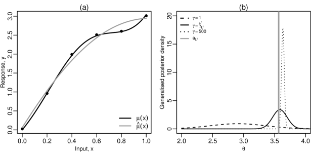
Figure 1: (a) Responses, $y_{1},\dots,y_{n}$ plotted against the inputs $x_{1},\dots,x_{n}$, and the functions $\mu(x)$ and $\hat{\mu}(x)$ plotted against $x$. (b) Generalized posterior densities plotted against $\theta$, under the $L^{2}$ loss function for differing values of $\gamma$. The vertical grey line shows the true value of $\theta_{L^{2}}$.

3 Automatic scaling

3.1 Introduction

As shown in Section 2.4, the scaling of the loss function is crucial. In this section, we propose automatic scaling procedures adapted from the composite likelihood literature (Ribatet et al., 2012).

Initially, suppose the mathematical model is exact. Then there exist $\boldsymbol{\theta}_{0}$ such that $\eta(\mathbf{x},\boldsymbol{\theta}_{0})=\mu(\mathbf{x})$ for all $\mathbf{x}\in\mathcal{X}$. Furthermore, suppose under (1) that the joint distribution of the errors $e_{1},\dots,e_{n}$ is completely specified and does not depend on any unknown nuisance parameters. The likelihood ratio statistic is $\Lambda_{0}(\boldsymbol{\theta}_{0};\mathbf{y},\mathbf{X})=2\left[\log\pi(\mathbf{y}|\hat{\boldsymbol{\theta}})-\log\pi(\mathbf{y}|\boldsymbol{\theta}_{0})\right]$, where $\hat{\boldsymbol{\theta}}$ are the maximum likelihood estimators of $\boldsymbol{\theta}_{0}$. Under certain conditions, $\Lambda_{0}(\boldsymbol{\theta}_{0};\mathbf{y},\mathbf{X})$ converges in distribution to $\chi^{2}_{p}$ as $n\to\infty$, and, in particular, $\mathrm{E}_{\mathbf{y}}\left[\Lambda_{0}(\boldsymbol{\theta}_{0};\mathbf{y},\mathbf{X})\right]\to p$.

Recall, from Section 2.3, the self-information loss is $\ell_{SI}(\boldsymbol{\theta};\mathbf{y})=-n^{-1}\log\pi(\mathbf{y}|\boldsymbol{\theta})$. Then the likelihood ratio statistic can be written

$$\Lambda_{0}(\boldsymbol{\theta}_{0};\mathbf{y})=2n\left[\ell_{SI}(\boldsymbol{\theta}_{0};\mathbf{y})-\ell_{SI}(\hat{\boldsymbol{\theta}};\mathbf{y})\right].$$ (9)

The idea is to choose the scaling of the loss so that, when replacing $\ell_{SI}$ and $\hat{\boldsymbol{\theta}}$ in (9) by the chosen scaled loss and the frequentist estimators, respectively, asymptotic properties of the resulting $\Lambda$ are maintained as those of $\Lambda_{0}$. The intuition behind this is for $\Lambda$ to behave like the likelihood ratio statistic would if the mathematical model was exact. We develop two such scalings. Magnitude scaling ensures that the asymptotic expectation of $\Lambda$ is equal to $p$, whereas curvature scaling ensures that $\Lambda$ converges in distribution to $\chi^{2}_{p}$.

The scaling procedures, described in Section 3.2, require some results on frequentist calibration under the $L^{2}$ and OLS loss functions which are established in Section SM1 in the Supplementary Material. Section SM1.1 states some common required conditions, and then Lemmas SM1.1 and SM1.2 (in Sections SM1.2 and SM1.3, respectively) state the required properties for frequentist $L^{2}$ and OLS calibration. We provide a brief summary of these results below. Similar to Wong et al. (2017), we consider the design $\mathbf{X}=\left\{\mathbf{x}_{1},\dots,\mathbf{x}_{n}\right\}$ to be fixed. Also, similar to Wong et al. (2017) and Xie and Xu (2021), we assume that the mathematical model $\eta(\mathbf{x},\boldsymbol{\theta})$ is computationally inexpensive to evaluate. If the mathematical model is a computationally expensive computer model, then it may be necessary to first perform a computer experiment, and then to use a surrogate model to predict the mathematical model (see, e.g. Gramacy, 2020, Section 1.2). In this case, we assume $\eta(\mathbf{x},\boldsymbol{\theta})$ to be the surrogate prediction, i.e. we calibrate the surrogate prediction rather than the mathematical model. Wong et al. (2017) and Xie and Xu (2021) justify this by stating that, in most cases, computer experiments are financially cheaper to run than physical experiments, and that the computer experiment is likely to be large enough to provide an accurate surrogate prediction of the underlying mathematical model. See Section 6.2 for an example.

Let $\ell_{M}(\boldsymbol{\theta};\mathbf{y})$ denote the loss function where $M$ can be either $L^{2}$ or OLS. Correspondingly, let $\hat{\boldsymbol{\theta}}_{M}$ be the the values of $\boldsymbol{\theta}\in\Theta$ that minimize $\ell_{M}(\boldsymbol{\theta};\mathbf{y})$. Furthermore, let

$$\hat{V}_{M}=\frac{\partial^{2}\ell_{M}(\hat{\boldsymbol{\theta}}_{M};\mathbf{y})}{\partial\boldsymbol{\theta}\partial\boldsymbol{\theta}^{\mathrm{\scriptscriptstyle T}}}\qquad\mbox{and}\qquad V=\frac{\partial^{2}L_{L^{2}}(\boldsymbol{\theta}_{L^{2}};\mathbf{y})}{\partial\boldsymbol{\theta}\partial\boldsymbol{\theta}^{\mathrm{\scriptscriptstyle T}}}.$$

Then Lemmas SM1.1 and SM1.2 give the following results.

1. As $n\to\infty$, $\hat{\boldsymbol{\theta}}_{M}\stackrel{{\scriptstyle p}}{{\to}}\boldsymbol{\theta}_{L^{2}}$.

2. As $n\to\infty$,

   $$\frac{\partial^{2}\ell_{M}(\boldsymbol{\theta}_{L^{2}};\mathbf{y})}{\partial\boldsymbol{\theta}\partial\boldsymbol{\theta}^{\mathrm{\scriptscriptstyle T}}}\stackrel{{\scriptstyle p}}{{\to}}V.$$

3. The loss $\ell_{M}(\boldsymbol{\theta};\mathbf{y})$ can be written

   $$\ell_{M}(\boldsymbol{\theta};\mathbf{y})=\ell_{M}(\hat{\boldsymbol{\theta}}_{M};\mathbf{y})+\frac{1}{2}\left(\boldsymbol{\theta}-\hat{\boldsymbol{\theta}}_{M}\right)^{\mathrm{\scriptscriptstyle T}}\hat{V}_{M}\left(\boldsymbol{\theta}-\hat{\boldsymbol{\theta}}_{M}\right)+r_{n}\left(\boldsymbol{\theta}-\hat{\boldsymbol{\theta}}_{M}\right),$$

   with $r_{n}(\mathbf{u})$ a function where there exist $\epsilon_{0},c_{0}>0$ such that for $n$ sufficiently large, $|r_{n}(\mathbf{u})|\leq c_{0}\left(\mathbf{u}^{T}\mathbf{u}\right)^{3/2}$ for $\mathbf{u}\in B_{\epsilon_{0}}(\mathbf{0})$, and $B_{\epsilon}(\mathbf{u})=\left\{\mathbf{u}\in\Theta:\mathbf{u}^{T}\mathbf{u}<\epsilon\right\}$.

4. As $n\to\infty$,

   $$\sqrt{n}\left(\hat{\boldsymbol{\theta}}_{M}-\boldsymbol{\theta}_{L^{2}}\right)\stackrel{{\scriptstyle d}}{{\to}}\mathrm{N}\left(\mathbf{0},V^{-1}W_{M}V^{-1}\right),$$

   where

   $$W_{L^{2}} = 4\sigma^{2}n\int_{\mathcal{X}}\frac{\eta(\mathbf{x},\boldsymbol{\theta}_{L^{2}})}{\partial\boldsymbol{\theta}}\mathbf{s}(\mathbf{x})^{\mathrm{\scriptscriptstyle T}}\mathrm{d}\mathbf{x}\int_{\mathcal{X}}\mathbf{s}(\mathbf{x})\frac{\eta(\mathbf{x},\boldsymbol{\theta}_{L^{2}})}{\partial\boldsymbol{\theta}^{\mathrm{\scriptscriptstyle T}}}\mathrm{d}\mathbf{x},$$

   $$W_{OLS} = \frac{4\sigma^{2}}{n}\sum_{i=1}^{n}\frac{\eta(\mathbf{x}_{i},\boldsymbol{\theta}_{L^{2}})}{\partial\boldsymbol{\theta}}\frac{\eta(\mathbf{x}_{i},\boldsymbol{\theta}_{L^{2}})}{\partial\boldsymbol{\theta}^{\mathrm{\scriptscriptstyle T}}}.$$

3.2 Magnitude and curvature scaling

3.2.1 Magnitude scaling

Magnitude scaling has loss, generalized likelihood and generalized posterior given by

$$\ell^{(mag)}_{M}(\boldsymbol{\theta};\mathbf{y}) = \gamma\ell_{M}(\boldsymbol{\theta};\mathbf{y}),$$

$$\pi_{G:M}^{(mag)}(\mathbf{y}|\boldsymbol{\theta}) = \exp\left[-n\ell^{(mag)}_{M}(\boldsymbol{\theta};\mathbf{y})\right]\qquad\mbox{and}\qquad\pi_{G:M}^{(mag)}(\boldsymbol{\theta}|\mathbf{y})\propto\pi_{G:M}^{(mag)}(\mathbf{y}|\boldsymbol{\theta})\pi(\boldsymbol{\theta}),$$

respectively, where $\gamma>0$ does not depend on $\boldsymbol{\theta}$ and $\pi(\cdot)$ is the density of the prior distribution for $\boldsymbol{\theta}_{L^{2}}$. Analogous to the likelihood ratio statistic in (9), define

$$\Lambda^{(mag)}_{M}\left(\boldsymbol{\theta}_{L^{2}};\mathbf{y}\right) = 2n\left[\ell^{(mag)}_{M}(\boldsymbol{\theta}_{L^{2}};\mathbf{y})-\ell^{(mag)}_{M}(\hat{\boldsymbol{\theta}}_{M};\mathbf{y})\right]$$

$$= 2n\gamma\left[\ell_{M}(\boldsymbol{\theta}_{L^{2}};\mathbf{y})-\ell_{M}(\hat{\boldsymbol{\theta}}_{M};\mathbf{y})\right].$$

The goal is to determine a value $\gamma_{M}^{*}>0$ for $\gamma$ to ensure the asymptotic expectation of $\Lambda^{(mag)}_{M}\left(\boldsymbol{\theta}_{L^{2}};\mathbf{y}\right)$ is $p$: the asymptotic expectation of the likelihood ratio statistic $\Lambda_{0}(\boldsymbol{\theta}_{0},\mathbf{y})$. By statement (c) from Section 3.1, $\Lambda^{(mag)}_{M}\left(\boldsymbol{\theta}_{L^{2}};\mathbf{y}\right)$ can be written

$$\Lambda^{(mag)}_{M}\left(\boldsymbol{\theta}_{L^{2}};\mathbf{y}\right)=n\gamma\left(\boldsymbol{\theta}_{L^{2}}-\hat{\boldsymbol{\theta}}_{M}\right)^{\mathrm{\scriptscriptstyle T}}\hat{V}_{M}\left(\boldsymbol{\theta}_{L^{2}}-\hat{\boldsymbol{\theta}}_{M}\right)+2n\gamma r_{n}\left(\boldsymbol{\theta}_{L^{2}}-\hat{\boldsymbol{\theta}}_{M}\right).$$

Then, by statements (a), (b) and (d) from Section 3.1, and since $\hat{V}_{M}\stackrel{{\scriptstyle p}}{{\to}}V$,

$$\mathrm{E}_{\mathbf{y}}\left[\Lambda^{(mag)}_{M}(\boldsymbol{\theta}_{L^{2}};\mathbf{y})\right]\to\gamma\mathrm{tr}\left(V^{-1}W_{M}\right),$$

as $n\to\infty$. Equating the asymptotic expectation of $\Lambda^{(mag)}_{M}(\boldsymbol{\theta}_{L^{2}};\mathbf{y})$ to $p$ yields

$$\gamma^{*}_{M}=\frac{p}{\mathrm{tr}\left(V^{-1}W_{M}\right)}.$$ (10)

Woody et al. (2019) considered a similar idea for scaling the $L^{2}$ loss under magnitude scaling. They specify $\gamma_{L^{2}}^{*}$ such that coverage of probability intervals from the general posterior distribution match the confidence intervals from the frequentist analysis. They estimate the value of $\gamma_{L^{2}}^{*}$ via a bootstrap procedure.

3.2.2 Curvature scaling

Curvature scaling has loss, generalized likelihood and generalized posterior given by

$$\ell_{M}^{(cur)}(\boldsymbol{\theta};\mathbf{y}) = \gamma^{*}_{M}\ell_{M}\left[\hat{\boldsymbol{\theta}}_{M}+\Gamma\left(\boldsymbol{\theta}-\hat{\boldsymbol{\theta}}_{M}\right);\mathbf{y}\right],$$ (11)

$$\pi_{G:M}^{(cur)}(\mathbf{y}|\boldsymbol{\theta}) = \exp\left[-n\ell^{(cur)}_{M}(\boldsymbol{\theta};\mathbf{y})\right]\qquad\mbox{and}\qquad\pi_{G:M}^{(cur)}(\boldsymbol{\theta}|\mathbf{y})\propto\pi_{G:M}^{(cur)}(\mathbf{y}|\boldsymbol{\theta})\pi(\boldsymbol{\theta}),$$

respectively, where $\Gamma\in G$ is a $p\times p$ matrix, independent of $\boldsymbol{\theta}$, and $G$ is the set of $p\times p$ real matrices. The definition of the curvature scaling loss function in (11) is slightly different to that proposed by Ribatet et al. (2012) in that we include the factor $\gamma^{*}_{M}$. As we show below, inclusion of $\gamma^{*}_{M}$ means that magnitude and curvature scaling coincide for $p=1$ calibration parameter. If $\hat{\boldsymbol{\theta}}_{M}+\Gamma\left(\boldsymbol{\theta}-\hat{\boldsymbol{\theta}}\right)\in\Theta$ for all $\boldsymbol{\theta}\in\Theta$ and $\Gamma\in G$, then $\hat{\boldsymbol{\theta}}_{M}=\arg\min_{\boldsymbol{\theta}\in\Theta}\ell_{M}^{(cur)}(\boldsymbol{\theta};\mathbf{y})$.

Define

$$\Lambda^{(cur)}_{M}\left(\boldsymbol{\theta}_{L^{2}};\mathbf{y}\right)=2n\left[\ell^{(cur)}_{M}(\boldsymbol{\theta}_{L^{2}};\mathbf{y})-\ell^{(cur)}_{M}(\hat{\boldsymbol{\theta}}_{M};\mathbf{y})\right].$$

By statement (c) from Section 3.1

$$\Lambda^{(cur)}_{M}\left(\boldsymbol{\theta}_{L^{2}};\mathbf{y}\right) = n\gamma^{*}_{M}\left(\boldsymbol{\theta}_{L^{2}}-\hat{\boldsymbol{\theta}}_{M}\right)^{\mathrm{\scriptscriptstyle T}}\Gamma^{\mathrm{\scriptscriptstyle T}}\frac{\partial^{2}\ell_{M}\left[\hat{\boldsymbol{\theta}}_{M}+\Gamma\left(\boldsymbol{\theta}_{L^{2}}-\hat{\boldsymbol{\theta}}_{M}\right);\mathbf{y}\right]}{\partial\boldsymbol{\theta}\partial\boldsymbol{\theta}^{\mathrm{\scriptscriptstyle T}}}\Gamma\left(\boldsymbol{\theta}_{L^{2}}-\hat{\boldsymbol{\theta}}_{M}\right)$$

$$\qquad\qquad+2n\gamma^{*}_{M}r_{n}(\boldsymbol{\theta}_{L^{2}}-\hat{\boldsymbol{\theta}}_{M}).$$

By statements (a) and (b) from Section 3.1,

$$\frac{\partial^{2}\ell_{M}\left[\hat{\boldsymbol{\theta}}_{M}+\Gamma\left(\boldsymbol{\theta}_{L^{2}}-\hat{\boldsymbol{\theta}}_{M}\right);\mathbf{y}\right]}{\partial\boldsymbol{\theta}\partial\boldsymbol{\theta}^{\mathrm{\scriptscriptstyle T}}}\stackrel{{\scriptstyle p}}{{\to}}V.$$ (12)

Curvature scaling involves specifying a $\Gamma_{M}^{*}\in G$ for $\Gamma$ such that $\Lambda^{(cur)}_{M}\left(\boldsymbol{\theta}_{L^{2}};\mathbf{y}\right)$ converges in distribution to $\chi^{2}_{p}$. By statement (d) from Section 3.1, this can be achieved by specifying $\Gamma^{*}_{M}$ such that

$$\gamma^{*}_{M}\Gamma_{M}^{*T}V\Gamma_{M}^{*}=VW_{M}^{-1}V,$$ (13)

i.e. the right-hand side of (13) is the inverse of the asymptotic variance matrix of $\hat{\boldsymbol{\theta}}_{M}$. A $\Gamma_{M}^{*}$ satisfying (13) is not unique but, following Ribatet et al. (2012), we let

$$\Gamma^{*}_{M}=Q_{M}^{-1}P_{M},$$ (14)

where $P_{M}$ and $Q_{M}$ are $p\times p$ matrices satisfying $P_{M}^{\mathrm{\scriptscriptstyle T}}P_{M}=VW_{M}^{-1}V$ and $Q_{M}^{\mathrm{\scriptscriptstyle T}}Q_{M}=\gamma^{*}_{M}V$.

If there is $p=1$ calibration parameter, then

$$\Gamma^{*}_{M}=\frac{\sqrt{V_{M}W_{M}^{-1}V_{M}}}{\sqrt{\gamma^{*}_{M}V_{M}}}=\frac{\sqrt{V_{M}W_{M}^{-1}}}{\sqrt{\gamma^{*}_{M}}}=1,$$

resulting in magnitude and curvature scaling coinciding.

3.2.3 Estimation of $\gamma_{M}^{*}$ and $\Gamma_{M}^{*}$

Note that $\gamma^{*}_{M}$ and $\Gamma^{*}_{M}$, given by (10) and (14) respectively, depend on unknown $\sigma^{2}$, $\mu(\mathbf{x})$ and $\boldsymbol{\theta}_{L^{2}}$. We use consistent estimators

$$\hat{\gamma}_{M}^{*}=\frac{p}{\mathrm{tr}\left(\hat{V}^{-1}_{M}\hat{W}_{M}\right)},\quad\mbox{and}\quad\hat{\Gamma}^{*}_{M}=\hat{Q}_{M}^{-1}\hat{P}_{M}$$

where $\hat{P}_{M}^{\mathrm{\scriptscriptstyle T}}\hat{P}_{M}=\hat{V}_{M}\hat{W}_{M}^{-1}\hat{V}_{M}$ and $\hat{Q}_{M}^{\mathrm{\scriptscriptstyle T}}\hat{Q}_{M}=\hat{\gamma}^{*}_{M}\hat{V}_{M}$ with

$$\hat{W}_{L^{2}} = 4\hat{\sigma}^{2}n\int_{\mathcal{X}}\frac{\partial\eta(\mathbf{x},\hat{\boldsymbol{\theta}}_{L^{2}})}{\partial\boldsymbol{\theta}}\mathbf{s}(\mathbf{x})^{\mathrm{\scriptscriptstyle T}}\mathrm{d}\mathbf{x}\int_{\mathcal{X}}\mathbf{s}(\mathbf{x})\frac{\partial\eta(\mathbf{x},\hat{\boldsymbol{\theta}}_{L^{2}})}{\partial\boldsymbol{\theta}}\mathrm{d}\mathbf{x}$$

$$\hat{W}_{OLS} = \frac{4\hat{\sigma}^{2}}{n}\sum_{i=1}^{n}\frac{\partial\eta(\mathbf{x}_{i},\hat{\boldsymbol{\theta}}_{OLS})}{\partial\boldsymbol{\theta}}\frac{\partial\eta(\mathbf{x}_{i},\hat{\boldsymbol{\theta}}_{OLS})}{\partial\boldsymbol{\theta}^{\mathrm{\scriptscriptstyle T}}}$$

and $\hat{\sigma}^{2}=\frac{\sum_{i=1}^{n}\left(y_{i}-\hat{\mu}(\mathbf{x}_{i})\right)^{2}}{n-\mathrm{tr}\left(S\right)}$, a consistent estimator of $\sigma^{2}$ (under condition SML4).

3.2.4 Illustration

To illustrate the scaling methods, consider the illustrative example in Section 2.4. For the set of responses shown in Figure 1(a), under magnitude scaling, we estimate $\hat{\gamma}_{L^{2}}^{*}=17.80$. Figure 1(b) shows the generalized posterior distribution under the $L^{2}$ loss function and $\hat{\gamma}_{L^{2}}^{*}$. The true $\theta_{L^{2}}$ now features in a region of relative high posterior density and the posterior mean is 3.5854, i.e. close to the target parameter value of $\theta_{L^{2}}=3.5653$.

3.3 Asymptotic behavior of the generalized posterior distribution

In this section, we consider theoretic properties of the generalized posterior distribution for $\boldsymbol{\theta}$ under $L^{2}$ and OLS loss functions, and the magnitude and curvature scaling described in Section 3.2.

First, let $\ell_{M}^{S}(\boldsymbol{\theta};\mathbf{y})$ denote the scaled loss where $M\in\left\{L^{2},\mbox{OLS}\right\}$ and $S\in\left\{(mag),(cur)\right\}$. The corresponding generalized posterior distribution is $\pi_{G:M}^{S}(\boldsymbol{\theta}|\mathbf{y})\propto\exp\left[-n\ell_{M}^{S}(\boldsymbol{\theta};\mathbf{y})\right]\pi(\boldsymbol{\theta})$. Similarly, the expected scaled loss is denoted $L_{M}^{S}(\boldsymbol{\theta})=\mathrm{E}\left[\ell_{M}^{S}(\boldsymbol{\theta};\mathbf{y})\right]$. The target parameter values are $\boldsymbol{\theta}_{M}^{S}=\arg\min_{\boldsymbol{\theta}\in\Theta}L_{M}^{S}(\boldsymbol{\theta})$. Note that, in general, $\boldsymbol{\theta}_{M}^{S}\neq\boldsymbol{\theta}_{L^{2}}$ for finite $n$. However, in Section SM2 we consider the asymptotic behavior of the generalized posterior distribution under loss $M$ and scaling $S$, including the behavior of $\boldsymbol{\theta}_{M}^{S}$. We provide a brief summary of the results below (all apply as $n\to\infty$).

1. The target parameter values $\boldsymbol{\theta}_{M}^{S}$ converge to $\boldsymbol{\theta}_{L^{2}}$, i.e. the target parameters of general Bayesian inference under both the $L^{2}$ and OLS losses converge to $\boldsymbol{\theta}_{L^{2}}$.

2. The generalized posterior distribution converges to a point mass at $\boldsymbol{\theta}_{L^{2}}$.

3. The generalized posterior distribution converges to $\mathrm{N}\left(\hat{\boldsymbol{\theta}}_{M},n^{-1}\Sigma_{S}^{-1}\right)$ where

   $$\Sigma_{(mag)}=\gamma^{*}_{M}V\qquad\mbox{and}\qquad\Sigma_{(cur)}=\gamma^{*}_{M}\Gamma^{*T}_{M}V\Gamma_{M}^{*}=VW_{M}^{-1}V.$$

3.4 Comparison of magnitude and curvature scaling

Following Ribatet et al. (2012), compared to the unscaled generalized posterior distribution, magnitude scaling changes the scale of the generalized posterior distribution whereas curvature scaling changes the scale and, for $p>1$, shape.

Furthermore, consider the result given by statement (c) in Section 3.3. Under loss function $M$ and magnitude scaling, the asymptotic generalized posterior variance of $\boldsymbol{\theta}_{L^{2}}$ is

$$n^{-1}\Sigma_{(mag)}=\frac{1}{n\gamma^{*}_{M}}V^{-1}=\frac{\mathrm{tr}\left(V^{-1}W_{M}\right)V^{-1}}{np}.$$

The determinant of the asymptotic variance $n^{-1}\Sigma_{(mag)}$ (a scalar measure of variability for a multivariate distribution; Wilkes 1932) is

$$|n^{-1}\Sigma_{(mag)}| = \frac{\mathrm{tr}\left(V^{-1}W_{M}\right)^{p}|V|^{-1}}{n^{p}p^{p}}$$

$$\geq \frac{|V^{-1}W_{M}||V|^{-1}}{n^{p}}$$

$$= \left|\frac{1}{n}V^{-1}W_{M}V^{-1}\right|,$$

where the inequality in the second line follows from the fact that the arithmetic mean of the eigenvalues of $V^{-1}W_{M}$ is greater or equal to the geometric mean. Therefore, under magnitude scaling, the asymptotic variability (as measured by the determinant) of the generalized posterior is greater than that of the frequentist estimator $\hat{\boldsymbol{\theta}}_{M}$. By contrast, under curvature scaling, the asymptotic generalized posterior variance is equal to that of $\hat{\boldsymbol{\theta}}_{M}$. This is a consequence of curvature scaling having greater flexibility in being able to change the scale and shape of the generalized posterior distribution.

In Sections 5 and 6, we compare the practical difference between magnitude and curvature scaling. We conclude that, in most cases, there is only minor difference. However, see Section 6.2 for an example where there is non-negligible difference between magnitude and curvature scaling. In this example, we demonstrate how the shape of the generalized posterior distribution, under curvature scaling, has been changed. In these cases, where the two scalings provide different results, we recommend curvature scaling due to its greater flexibility, as described above.

4 Comparison of OLS calibration and traditional Bayesian inference under normal errors

In this section, we consider the apparent similarity between general Bayesian calibration under the OLS loss and traditional Bayesian inference under the assumption that the errors $e_{1},\dots,e_{n}$ are an independent and identically distributed sample from a normal distribution with mean zero and constant variance (denoted by $\tau^{2}$ to distinguish it from the true error variance $\sigma^{2}$).

The likelihood is $\pi(\mathbf{y}|\boldsymbol{\theta},\tau^{2})=\left(2\pi\right)^{-\frac{n}{2}}\left(\tau^{2}\right)^{-\frac{n}{2}}\exp\left[-\frac{n\ell_{OLS}(\boldsymbol{\theta};\mathbf{y})}{2\tau^{2}}\right]$. The corresponding expected self-information loss is

$$L_{SI}(\boldsymbol{\theta},\tau^{2})=\mathrm{E}_{\mathbf{y}}\left[-\frac{1}{n}\log\pi(\mathbf{y}|\boldsymbol{\theta},\tau^{2})\right]=\frac{1}{2}\log(2\pi)+\frac{1}{2}\log\tau^{2}+\frac{1}{2\tau^{2}}\mathrm{E}_{\mathbf{y}}\left[\ell_{OLS}(\boldsymbol{\theta};\mathbf{y})\right].$$

Following Section 2.3, the target values $\boldsymbol{\theta}_{SI}$ and $\tau^{2}_{SI}$ are given by minimizing $L_{SI}(\boldsymbol{\theta},\tau^{2})$ with respect to $\boldsymbol{\theta}$ and $\tau^{2}$.

Assume conditions SMC1-SMC6 and SMO1-SMO7, then the proof of Lemma 2 in Wong et al. (2017) shows that $\ell_{OLS}(\boldsymbol{\theta};\mathbf{y})$ converges uniformly (with respect to $\boldsymbol{\theta}$) to $L_{L^{2}}(\boldsymbol{\theta})+\sigma^{2}$ in probability, as $n\to\infty$. Hence $L_{SI}(\boldsymbol{\theta},\tau^{2})$ converges uniformly to $\frac{1}{2}\log(2\pi)+\frac{1}{2}\log\tau^{2}+\frac{1}{2\tau^{2}}\left[L_{L^{2}}(\boldsymbol{\theta})+\sigma^{2}\right]$, and therefore $\boldsymbol{\theta}_{SI}\to\boldsymbol{\theta}_{L^{2}}$. This means that the asymptotic target parameter values for the calibration parameters of traditional Bayesian inference match those of general Bayesian $L^{2}$ and OLS calibration.

However, the target parameter value, $\tau^{2}_{SI}$, for $\tau^{2}$ is

$$\tau^{2}_{SI}=\mathrm{E}_{\mathbf{y}}\left[\ell_{OLS}(\boldsymbol{\theta}_{SI};\mathbf{y})\right]=\ell_{OLS}(\boldsymbol{\theta};\boldsymbol{\mu})+\sigma^{2}\to L_{L^{2}}(\boldsymbol{\theta}_{L^{2}})+\sigma^{2}.$$ (15)

Therefore the target value for $\tau^{2}$ has $\tau^{2}_{SI}\geq\sigma^{2}$. In the limit, equality occurs if and only if $L_{L^{2}}(\boldsymbol{\theta}_{L^{2}})=0$, i.e. the mathematical model is exact.

Now consider the conditional (given $\tau^{2}$) traditional Bayesian posterior distribution of $\boldsymbol{\theta}$ given by $\pi(\boldsymbol{\theta}|\mathbf{y},\tau^{2})\propto\pi(\mathbf{y}|\boldsymbol{\theta},\tau^{2})\pi(\boldsymbol{\theta}|\tau^{2})$. Suppose $\pi(\boldsymbol{\theta}|\tau^{2})$ is continuous and positive at $\boldsymbol{\theta}=\boldsymbol{\theta}_{L^{2}}$. Theorem 4 of Miller (2021) implies a limiting normal distribution of $\mathrm{N}\left(\hat{\boldsymbol{\theta}}_{OLS},n^{-1}\Sigma_{SI}^{-1}\right)$ where $\Sigma_{SI}=V/2\tau^{2}$. Therefore, the asymptotic variance of the conditional posterior of $\boldsymbol{\theta}$ is proportional to $\tau^{2}$. Thus if traditional Bayesian calibration targets a value, $\tau^{2}_{SI}$, of $\tau^{2}$ greater than $\sigma^{2}$, then we expect the variance of the conditional posterior of $\boldsymbol{\theta}$ to be inflated. From (15), the amount of inflation is controlled by the relative magnitudes of $L_{L^{2}}(\boldsymbol{\theta}_{L^{2}})$ and $\sigma^{2}$. We investigate this issue empirically in Sections 5 and 6, where traditional Bayesian calibration is compared to general Bayesian calibration.

5 Simulation study

5.1 Introduction

In this section we consider synthetic, but illustrative, examples to investigate the long-run performance of different calibration methods for finite physical experiment size $n$. Throughout, five different calibration approaches are applied as follows:

• general Bayesian calibration under the $L^{2}$ loss, with (1) magnitude and (2) curvature (if $p>1$) scaling;

• general Bayesian calibration under the OLS loss, with (3) magnitude and (4) curvature (if $p>1$) scaling; and

• (5) traditional Bayesian inference under normal errors.

There are four configurations (listed in Section 5.2 and labelled Configurations 1 to 4), each defined by a mathematical model, and true physical process. In each configuration, the true physical process $\mu(\mathbf{x})$ is known. Correspondingly the true values of $\boldsymbol{\theta}_{L^{2}}$ can be determined. We generate responses from the true physical process via (1), where the distribution of $e_{i}$ is normal with mean zero and variance $\sigma^{2}$. We then implement the five calibration approaches listed above. We repeat this process 500 times for a range of different values of $n$. The calibration approaches are compared using the sample mean of the generalized posterior mean and log standard deviation, and the coverage of 95% probability intervals for the elements of $\boldsymbol{\theta}_{L^{2}}$. The probability intervals are computed as highest (generalized) posterior density intervals.

Note that practical details on how to compute the generalized posterior distribution are given in Section SM3. These include how to (a) evaluate the $L^{2}$ loss $\ell_{L^{2}}(\boldsymbol{\theta};\mathbf{y})$ and (b) sample from the generalized posterior distribution using Markov chain Monte Carlo (MCMC) methods. The R code used to perform the simulation studies is included in the Supplementary Material.

5.2 Configurations

The following configurations have been used by Wong et al. (2017), Gu and Wang (2018) and Xie and Xu (2021) to validate methods for calibrating mathematical models.

Configuration 1

The mathematical model, with $k=1$ and $p=2$, is

$$\eta(x,\boldsymbol{\theta})=7\left[\sin\left(2\pi\theta_{1}-\pi\right)\right]^{2}+2\left[\left(2\pi\theta_{2}-\pi\right)^{2}\sin\left(2\pi x-\pi\right)\right],$$

where $\boldsymbol{\theta}=\left(\theta_{1},\theta_{2}\right)^{T}$. The physical process is $\mu(x)=\eta(x,\boldsymbol{\theta}_{0})$ with $\boldsymbol{\theta}_{0}=\left(0.2,0.3\right)^{T}$, i.e. the mathematical model is exact. It follows that $\boldsymbol{\theta}_{L^{2}}=\boldsymbol{\theta}_{0}$. The error variance is $\sigma^{2}=0.2^{2}$, $x_{1},\dots,x_{n}$ are equally-spaced on $\mathcal{X}$, and we consider $n=25,50,\dots,200$. Xie and Xu (2021) considered $n=50$ with a random design. The prior distribution for $\boldsymbol{\theta}_{L^{2}}$ is such that the elements are independent with $\theta_{L^{2},1}\sim\mathrm{U}(0,0.25)$ and $\theta_{L^{2},2}\sim\mathrm{U}(0,0.5)$.

Configuration 2

The mathematical model, with $k=1$ and $p=1$, is

$$\eta(x,\theta)=\sin\left(5\theta x\right)+5x$$

and the physical process is

$$\mu(x)=5x\cos\left(15x/2\right)+5x.$$

The value of $\theta$ minimizing $L_{L^{2}}(\theta)$ can be found numerically as $\theta_{L^{2}}=1.8772$. The error variance is $\sigma^{2}=0.2^{2}$, $x_{1},\dots,x_{n}$ are equally-spaced on $\mathcal{X}$, and we consider $n=30,60,\dots,240$. Xie and Xu (2021) and Gu and Wang (2018) considered $n=30$. The prior distribution for $\theta_{L^{2}}$ is $\mathrm{U}\left(0,3\right)$.

Configuration 3

The mathematical model, with $k=1$ and $p=1$, true physical process, error variance, and corresponding value of $\theta_{L^{2}}$ are given in the illustrative example in Section 2.4. We consider two different designs: (i) $x_{1},\dots,x_{n}$ are equally-spaced on $\mathcal{X}$; and (ii) $x_{1},\dots,x_{n}$ are equally-spaced on $\mathcal{X}^{\prime}=[0,0.8]$. Xie and Xu (2021) and Plumlee (2017) considered $n=17$ with data-generation specifications (i) and (ii), respectively.

For design specification (ii), the feature that the space on which the inputs $x_{1},\dots,x_{n}$ are selected, $\mathcal{X}^{\prime}$, is a subset of $\mathcal{X}$ represents the situation where the inputs in an experiment cannot be selected from some regions of $\mathcal{X}$. If we define an $L^{2}$ loss on $\mathcal{X}^{\prime}$, i.e.

$$L^{\prime}_{L^{2}}(\theta)=\int_{\mathcal{X}^{\prime}}\left(\mu(x)-\eta(x,\theta)\right)^{2}\mathrm{d}x,$$

then its minimizer is

$$\theta^{\prime}_{L^{2}}=\arg\min L^{\prime}_{L^{2}}(\theta)=4.0514.$$

By Theorem SM2.1, this is the target parameter for OLS calibration.

Configuration 4

The mathematical model, with $k=2$ and $p=3$, is

$$\eta(\mathbf{x},\boldsymbol{\theta})=7\sin^{2}\left(2\pi\theta_{1}-\pi\right)+2\left(2\pi\theta_{2}-\pi\right)^{2}\sin\left(2\pi x_{1}-\pi\right)+6\theta_{3}\left(x_{2}-\frac{1}{2}\right),$$

and the physical process is

$$\mu(\mathbf{x})=\eta(\mathbf{x},\boldsymbol{\theta}_{0})+\cos\left(2\pi x_{1}-\pi\right)+2\left(x_{2}^{2}-x_{2}+\frac{1}{6}\right),$$

where $\boldsymbol{\theta}_{0}=\left(0.2,0.3,0.8\right)^{T}$. The values of $\boldsymbol{\theta}$ that minimize $L_{L^{2}}(\boldsymbol{\theta})$ are $\boldsymbol{\theta}_{L^{2}}=\boldsymbol{\theta}_{0}$. Following Wong et al. 2017,

$$\sigma^{2}=\frac{1}{10}\int_{\mathcal{X}}\left[\mu(\mathbf{x})-\int_{\mathcal{X}}\mu(\mathbf{x})^{2}\mathrm{d}\mathbf{x}\right]^{2}\mathrm{d}\mathbf{x}=0.7430.$$

The inputs $\mathbf{x}_{1},\dots,\mathbf{x}_{n}$ are the points of a maximum projection Latin hypercube design (Joseph et al., 2015) found using the R package MaxPro (Ba and Joseph, 2018). We consider $n=30,40,\dots,100,150,\dots,400$. Wong et al. (2017) considered $n=50$. We assume the following independent prior distributions for the elements of $\boldsymbol{\theta}_{L^{2}}$:

$$\theta_{L^{2},1}\sim\mathrm{U}[0,0.25];\qquad\theta_{L^{2},2}\sim\mathrm{U}[0,0.5];\qquad\theta_{L^{2},3}\sim\mathrm{U}[0,1];$$

following the parameter spaces considered by Wong et al. (2017).

5.3 Results

Configuration 1

The results for Configuration 1 are summarized by Figure 2 for $\theta_{1}$ (left-hand panels) and $\theta_{2}$ (right-hand). The first and second rows show the mean (over the 500 replications) of the generalized posterior mean and log standard deviation plotted against $n$. The third rows show the coverage of the 95% probability intervals plotted against $n$. In this case, when the mathematical model is exact, all five methods perform similarly except for the smallest value of $n=25$. Here, traditional Bayesian inference has coverage closer to the nominal 95% than the general Bayesian approaches. Finally, there is negligible difference between magnitude and curvature scaling.

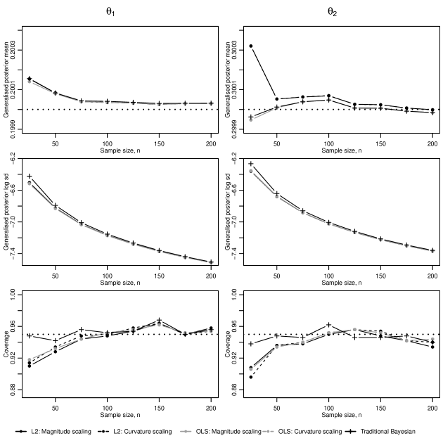
Figure 2: Results for Configuration 1 for $\theta_{1}$ (left-hand panels) and $\theta_{2}$ (right-hand panels). The first and second rows show the sample mean (over the 500 repetitions of the simulation study) generalized posterior mean and log standard deviation, respectively, plotted against $n$ for the five different calibration approaches. The third row shows the coverage of 95% probability intervals plotted against $n$.

Configuration 2

The results for Configuration 2 are summarized by column (a) of Figure 3. The organisation of the figure rows are identical to those in Figure 2. The posterior mean for general Bayesian calibration under the $L^{2}$ loss is closer to the true $\theta_{L^{2}}$ than under the OLS loss. This bias for the OLS loss causes significant under-coverage of the probability intervals evident in the last row. As expected, from Section 4, since the mathematical model is inexact, the posterior standard deviation under traditional Bayesian calibration is inflated (when compared to the general Bayesian approaches). We can provide some further insight here by stating that $L_{L^{2}}(\theta_{L^{2}})=2.866$ with $\sigma^{2}=0.2^{2}=0.04$, so the target response variance for traditional Bayesian calibration is $\tau^{2}_{SI}=2.906$. This causes the over-coverage of the probability intervals for traditional Bayesian calibration.

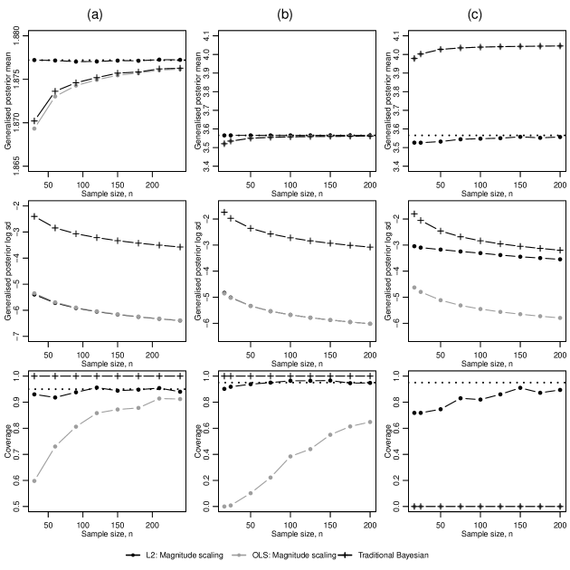
Figure 3: Results for (a) Configuration 2; (b) Configuration 3 with design specification (i) $\mathcal{X}=[0,1]$; and (c) Configuration 3 with design specification (ii) $\mathcal{X}^{\prime}=[0,0.8]$. The first and second rows show the sample mean (over the 500 repetitions of the simulation study) generalized posterior mean and log standard deviation, respectively, plotted against $n$ for the five different calibration approaches. The third row shows the coverage of 95% probability intervals plotted against $n$.

Configuration 3

The results for Configuration 3 are summarized by columns (b) and (c) of Figure 3, for designs with support $\mathcal{X}=[0,1]$ and $\mathcal{X}^{\prime}=[0,0.8]$, respectively. The organisation of the figure rows are identical to those in Figure 2. The scale of the $y$-axis for the first row of Figure 3 (b) and (c) is the same to aid comparison.

When the support for the design is $\mathcal{X}=[0,1]$, the results are similar to those from Configuration 2. The posterior mean and probability interval coverage for general Bayesian calibration under the $L^{2}$ loss are close to $\boldsymbol{\theta}_{L^{2}}$ and 95%, respectively. There is decreasing bias in the posterior mean for general Bayesian calibration under the OLS loss and traditional Bayesian calibration. This leads to probability interval under-coverage for the OLS loss. However, the inflated posterior variance under traditional Bayesian calibration leads to over-coverage. This can be seen from the fact that $L_{L^{2}}(\theta_{L^{2}})=0.1387$, $\sigma^{2}=0.02^{2}$, leading to $\tau^{2}_{SI}=0.1391$.

Now consider when the support for the design is $\mathcal{X}^{\prime}=[0,0.8]$. The posterior mean and interval coverage for general Bayesian calibration under the $L^{2}$ loss does converge to $\theta_{L^{2}}$ and 95%, respectively. However, the convergence is slower than for when the design support was $\mathcal{X}=[0,1]$. As expected, the posterior mean for general Bayesian calibration under the OLS loss and for traditional Bayesian calibration converges to $\theta_{L^{2}}^{\prime}=4.0514$. This bias (between $\theta_{L^{2}}$ and $\theta_{L^{2}}^{\prime}$) causes 0% coverage of the intervals, even accounting for the inflated posterior variance under traditional Bayesian calibration.

Configuration 4

The results for Configuration 4 are summarized by Figure 4. The three columns correspond to $\theta_{1}$, $\theta_{2}$ and $\theta_{3}$, respectively. The organisation of the figure rows are identical to those for Configurations 1 to 3.

The first conclusion to draw is that there is negligible difference between magnitude and curvature scaling. The generalized posterior means of $\boldsymbol{\theta}$ converge to the true values $\boldsymbol{\theta}_{L^{2}}$ as $n$ increases. For large $n$, the mean generalized posterior means for OLS and traditional Bayesian inference become close, as expected from Section SM3. Also, as expected from Section SM3, the mean posterior standard deviation of traditional Bayesian inference is larger than under the $L^{2}$ and OLS calibration approaches. This leads to over-coverage of the probability intervals for traditional Bayesian inference. However, the posterior variance inflation is not as significant as in Configurations 2 and 3. This can be seen from the fact that in Configuration 4, $L_{L^{2}}(\boldsymbol{\theta}_{L^{2}})=0.5222$, $\sigma^{2}=0.7430$, leading to $\tau^{2}_{SI}=1.265$, i.e. $L_{L^{2}}(\boldsymbol{\theta}_{L^{2}})$ does not dominate $\sigma^{2}$ as it does in Configurations 2 and 3.

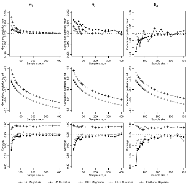
Figure 4: Results for Configuration 4 for $\theta_{1}$ (left column), $\theta_{2}$ (centre) and $\theta_{3}$ (right). The first and second rows show the sample mean (over the 500 repetitions of the simulation study) generalized posterior mean and log standard deviation of $\theta$ plotted against $n$ under $L^{2}$ and OLS calibration and under magnitude and curvature scaling. The third row shows the coverage of 95% probability intervals plotted against $n$.

5.4 Summary

Overall, general Bayesian calibration under the $L^{2}$ loss performed well, even for small $n$. By this, it is meant that the generalized posterior mean was close to the target parameter values $\boldsymbol{\theta}_{L^{2}}$ and coverage of probability intervals were close to the nominal value. There was evidence (see Configurations 2 and 3) to support the use of the $L^{2}$ loss over OLS in terms of the mean posterior mean and coverage of probability intervals being significantly closer to the true value of $\theta_{L^{2}}$ and 95%, respectively, for all but very large $n$. For both loss functions, there was negligible difference, in terms of long-run performance, between curvature and magnitude scaling.

Traditional Bayesian inference performs similarly to (if not better than) general Bayesian calibration when the mathematical model is exact (see Configuration 1) but the posterior distribution for the calibration parameters exhibits inflated posterior variance when the mathematical model is not true (see Configurations 2 to 4) manifesting itself in over-coverage of the probability intervals. As predicted from Section 4, the degree of inflated posterior variance is controlled by the relative magnitude of $\sigma^{2}$ and $L_{L^{2}}(\boldsymbol{\theta}_{L^{2}})$.

6 Examples

We now consider three real examples, specifically: ion channels of cardiac cells (Section 6.1), radiative shock hydrodynamics (Section 6.2), and wiffle balls (Section SM4.2). In each example, we implement the five different calibration methods listed in Section 5.1. An MCMC sample of size 100,000 is generated from each generalized posterior distribution. Recall, that details on how to compute the generalized posterior distribution in practice (including MCMC sampling) are given in Section SM3. R code implementing the calibration in each example is provided in the Supplementary Material.

6.1 Ion channels of cardiac cells

The following example comes from Plumlee (2017) and Xie and Xu (2021). We use this example to compare the proposed approaches to the state-of-the-art, alternative Bayesian $L^{2}$ calibration of Xie and Xu (2021) briefly described in Section 2.2.3.

The data were collected to learn about ion channels of cardiac cells. The experiment involved measuring the response (the current through sodium channels in the cardiac cell membrane) required to maintain a fixed potential at a given time (the $k=1$ input). We consider a subset of the data as considered by Plumlee (2017) and Xie and Xu (2021). This consists of $n=19$ measurements. Following Plumlee (2017), we set the input $x$ to be the logarithm of time scaled to $\mathcal{X}=[0,1]$, where the original log-time measurements were on the interval $[-1.75,3]$.

The mathematical model is

$$\eta(x,\boldsymbol{\theta})=\mathbf{e}_{1}^{\mathrm{\scriptscriptstyle T}}\mathrm{mexp}\left[A(x,\boldsymbol{\theta})\right]\mathbf{e}_{4}.$$ (16)

In (16), $\mathrm{mexp}[\cdot]$ denotes the matrix exponential, $\mathbf{e}_{1}=(1,0,0,0)^{\mathrm{\scriptscriptstyle T}}$, $\mathbf{e}_{4}=(0,0,0,1)^{\mathrm{\scriptscriptstyle T}}$, $\boldsymbol{\theta}=\left(\theta_{1},\dots,\theta_{3}\right)^{\mathrm{\scriptscriptstyle T}}$ (i.e. $p=3$), and $A(x,\boldsymbol{\theta})=\exp(x)T(\boldsymbol{\theta})$ where $T(\boldsymbol{\theta})$ is a $4\times 4$ matrix with $T(\boldsymbol{\theta})_{11}=-\theta_{2}-\theta_{3}$, $T(\boldsymbol{\theta})_{22}=T(\boldsymbol{\theta})_{33}=-\theta_{1}-\theta_{2}$, $T(\boldsymbol{\theta})_{44}=\theta_{1}$, $T(\boldsymbol{\theta})_{12}=T(\boldsymbol{\theta})_{23}=T(\boldsymbol{\theta})_{34}=\theta_{1}$, $T(\boldsymbol{\theta})_{21}=T(\boldsymbol{\theta})_{32}=T(\boldsymbol{\theta})_{43}=\theta_{2}$, and all other elements equal to zero. The prior distribution for $\boldsymbol{\theta}_{L^{2}}$ is such that the elements are independent with $\theta_{L^{2},1}\sim\mathrm{U}[0,10]$, $\theta_{L^{2},2}\sim\mathrm{U}[0,10]$ and $\theta_{L^{2},3}\sim\mathrm{U}[0,10]$. Figure 5(a) shows a plot of the observed values of the normalized current ($y_{1},\dots,y_{n}$) against logarithm of time.

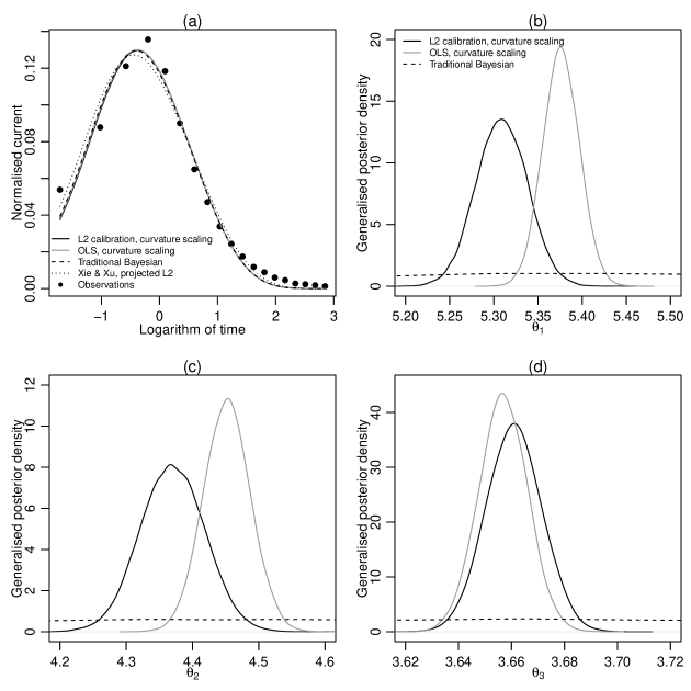
Figure 5: Results for the ion channel example. Panel (a) shows a plot of the observed values of the normalized current ($y_{1},\dots,y_{n}$) against logarithm of time ($x_{1},\dots,x_{n}$). It also shows the mean of $\eta(\boldsymbol{\theta}_{i},x)$ plotted against $x$ for each of $L^{2}$ and OLS calibration for both scaling approaches, where $\left\{\boldsymbol{\theta}\right\}_{i=1}^{M}$ denotes the sample from the generalized posterior distribution. Panels (b), (c) and (d) show the generalized posterior densities for $\theta_{1}$, $\theta_{2}$ and $\theta_{3}$, respectively.

Table 1 shows the posterior mean and standard deviation for each of the $p=3$ calibration parameters for each of the five calibration methods, in addition to the corresponding statistics taken from Xie and Xu (2021) for the same dataset. Similar to the simulation studies in Section 5, there is very small difference between magnitude and curvature scaling.

	$L^{2}$	$L^{2}$	OLS	OLS	Traditional	Xie & Xu
	magnitude	curvature	magnitude	curvature	Bayesian	projected $L^{2}$
$\theta_{1}$	5.31	5.31	5.38	5.38	5.47	6.01
	(0.0212)	(0.0290)	(0.0195)	(0.0205)	(0.424)	(1.20 $\times 10^{-5}$)
$\theta_{2}$	4.37	4.37	4.45	4.45	4.60	5.58
	(0.0401)	(0.0485)	(0.0331)	(0.0351)	(0.716)	(6.00 $\times 10^{-6}$)
$\theta_{3}$	3.66	3.66	3.66	3.66	3.66	3.501
	(0.0138)	(0.0102)	(0.00896)	(0.00908)	(0.187)	(6.00 $\times 10^{-6}$)
OLS	3.39	3.39	3.38	3.38	3.40	3.98
($\times 10^{-5}$)

Table 1: Results for the ion channel example. Top: Generalized posterior mean (standard deviation) for $\theta_{1}$, $\theta_{2}$ and $\theta_{3}$ for the five different calibration methods considered in this paper and Xie and Xu (2021)’s projection approach. Bottom: OLS statistic evaluated at the posterior mean for all methods.

Figures 5(b)-(d) show the posterior densities for $\theta_{1}$, $\theta_{2}$ and $\theta_{3}$, respectively, for general Bayesian calibration under the $L^{2}$ and OLS loss functions with curvature scaling (magnitude scaling is omitted for clarity), and traditional Bayesian calibration. There is reasonable agreement between the general Bayesian calibration methods with overlap of the posterior densities. The posterior distribution under traditional Bayesian calibration exhibits very high variance. Unlike the simulation studies we cannot compare $L_{L^{2}}(\boldsymbol{\theta}_{L^{2}})$ and $\sigma^{2}$. However, we can estimate these values by $\ell_{L^{2}}(\hat{\boldsymbol{\theta}}_{L^{2}})=3.712\times 10^{-5}$ and $\hat{\sigma}^{2}=1.029\times 10^{-7}$, respectively. Hence, we estimate $L_{L^{2}}(\boldsymbol{\theta}_{L^{2}})$ to be two orders of magnitude greater than $\sigma^{2}$, thus explaining the inflated posterior variance.

The summary statistics in Table 1, from Xie and Xu (2021), shows that their posterior distribution is very different (both in terms of location and scale) to those from the methods considered in this paper. To investigate this we calculate the OLS loss function, $\ell_{OLS}\left(\boldsymbol{\theta};\mathbf{y}\right)$, for $\boldsymbol{\theta}$ equal to the posterior mean under the six different methods under consideration. Comparison using the OLS loss function was chosen since this does not rely on $\hat{\mu}(\cdot)$. The values of the OLS loss are shown in the lower part of Table 1. The methods considered in this paper result in smaller OLS loss than that in Xie and Xu (2021). However, the difference between the methods on the response scale is quite small. This is evidenced by Figure 5(a) which includes $\eta\left(x,\boldsymbol{\theta}\right)$ plotted against $x$ where $\boldsymbol{\theta}$ is given by the posterior mean under the different methods (magnitude scaling omitted for clarity).

6.2 Radiative shock hydrodynamics

The application in this example is described in Gramacy (2020, Section 2.2). The data were collected to learn about radiative shocks which arise from astrophysical phenomena. The physical experiment involves a high energy laser irradiating a beryllium disk at the front of a tube filled with Xenon gas. This causes a high speed shock wave to travel down the tube. The response is the shock location, i.e. the distance travelled down the tube by the shock wave in a predetermined time.

The physical experiment consists of $n=20$ runs and $k=4$ inputs are varied: laser energy (in $[3750,3889.6]$ J), Xenon gas pressure (in $[1.032,1.311]$ atm), tube diameter (in $[0.575,1.150]$ mm) and time (in $[13,28]$ ns). All ranges for input variables are on the original scale. Let $x_{1},x_{2},x_{3},x_{4}$ denote the inputs laser energy, Xenon gas pressure, tube diameter and time scaled to $[0,1]$, respectively.

The mathematical model is given by the predictive mean of a Gaussian process surrogate model fitted to the input and output of a computer experiment. The computer model outputs a theoretical prediction of the shock location based on 10 computer model inputs. The computer model inputs are the $p=2$ calibration parameters (electron flux limiter, $\theta_{1}\in[0.04,0.1]$; and energy scale factor, $\theta_{2}\in[0.4,1.1]$), the $k=4$ inputs varied in the physical experiment and a further four variables. The additional four variables are held fixed in the physical experiment but varied in the computer experiment.

The computer experiment consists of nearly 26,500 runs. This is too large to feasibly fit a Gaussian process surrogate model. Instead, we create a sub-design of 2650 runs, i.e. 10% of the original design. This is accomplished by constructing a maximin Latin hypercube (LH) design of 500 points in the 10 computer model input variables. Then for each point in the LH design, we find the nearest design point (by Euclidean distance) in the computer experiment design. The Gaussian process surrogate model was implemented using the R package RobustGASP using a Gaussian correlation function. Based on an independent test design of 500 runs, the Gaussian process model provides good predictions. Figure SM7(a) shows a plot of surrogate predictions against true mathematical model responses for the test design points. The corresponding root mean relative squared error is $0.00171$.

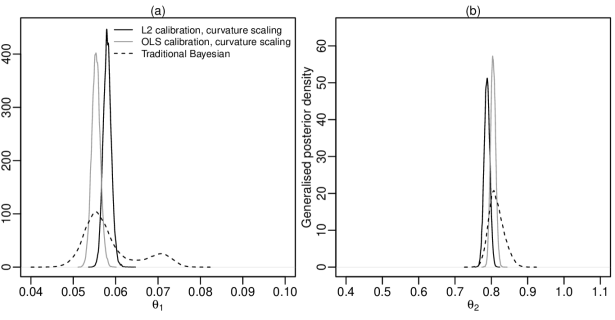
Figure 6: Results from the radiative shock hydrodynamics example. The plots show the generalized posterior density of $\theta_{1}$ (a) and $\theta_{2}$ (b), for $L^{2}$ and OLS calibration under curvature scaling, and traditional Bayesian calibration.

Figure SM8 shows a plot of the design points, $\mathbf{x}_{1},\dots\mathbf{x}_{n}$, of the physical experiment. The design points do not cover $\mathcal{X}$ as well as, for example, a LH design. This impacts the fit of the non-parametric regression model. We found the fit could be improved significantly (based on leave-one-out diagnostics) by including an intercept and a linear term for scaled time, $x_{4}$. Let $\mathbf{f}(\mathbf{x})=(1,x_{4})^{\mathrm{\scriptscriptstyle T}}$ and let $F$ be the $n\times 2$ matrix with $i$th row given by $\mathbf{f}(\mathbf{x}_{i})^{\mathrm{\scriptscriptstyle T}}$, for $i=1,\dots,n$. Furthermore, let $\hat{\boldsymbol{\beta}}=(F^{\mathrm{\scriptscriptstyle T}}F)^{-1}F^{\mathrm{\scriptscriptstyle T}}\mathbf{y}$ be the ordinary least squares estimators of the parameters associated with the linear model given by $\mathbf{f}(\mathbf{x})^{\mathrm{\scriptscriptstyle T}}$, and let $H=F(F^{\mathrm{\scriptscriptstyle T}}F)^{-1}F^{\mathrm{\scriptscriptstyle T}}$ be the hat matrix. Now

$$\hat{\mu}(\mathbf{x})=\mathbf{f}(\mathbf{x})^{\mathrm{\scriptscriptstyle T}}\hat{\boldsymbol{\beta}}+\sum_{i=1}^{n}s_{i}(\mathbf{x})\left(y_{i}-\mathbf{f}(\mathbf{x}_{i})^{\mathrm{\scriptscriptstyle T}}\hat{\boldsymbol{\beta}}\right),$$

where $\boldsymbol{\rho}$ are estimated as $\hat{\boldsymbol{\rho}}=\arg\min\mathbf{y}^{\mathrm{\scriptscriptstyle T}}\left(I_{n}-H-S-SH\right)^{2}\mathbf{y}/\left[1-2/n-\mathrm{tr}(S)/n\right]^{2}$. The estimators $\hat{W}_{L^{2}}$ and $\hat{\sigma}^{2}$ are adjusted to

$$\hat{W}_{L^{2}} = 4\hat{\sigma}^{2}n\int_{\mathcal{X}}\frac{\partial\eta(\mathbf{x},\hat{\boldsymbol{\theta}}_{L^{2}})}{\boldsymbol{\theta}}\left[\mathbf{s}(\mathbf{x})+F(F^{\mathrm{\scriptscriptstyle T}}F)^{-1}\mathbf{f}(\mathbf{x})\right]^{\mathrm{\scriptscriptstyle T}}\mathrm{d}\mathbf{x}$$

$$\qquad\times\int_{\mathcal{X}}\left[\mathbf{s}(\mathbf{x})+F(F^{\mathrm{\scriptscriptstyle T}}F)^{-1}\mathbf{f}(\mathbf{x})\right]\frac{\partial\eta(\mathbf{x},\hat{\boldsymbol{\theta}}_{L^{2}})}{\boldsymbol{\theta}^{\mathrm{\scriptscriptstyle T}}}\mathrm{d}\mathbf{x}$$

$$\hat{\sigma}^{2} = \frac{\sum_{i=1}^{n}\left(y_{i}-\hat{\mu}(\mathbf{x}_{i})\right)^{2}}{n-2-\mathrm{tr}(S)},$$ (17)

respectively.

Following Gramacy (2020, Chapter 9), the prior distribution for $\boldsymbol{\theta}_{L^{2}}$ is such that the elements are independent with each element having a Beta distribution (with both shape parameters equal to 1.5) scaled to $[0.04,0.1]$ for $\theta_{1}$ and $[0.4,1.10]$ for $\theta_{2}$.

Table 2 shows the posterior mean and standard deviation for $\theta_{1}$ and $\theta_{2}$ for the five different calibration methods. Compared to the other examples, there is some difference between magnitude and curvature scaling for general Bayesian calibration, under the $L^{2}$ loss. This difference manifests itself in the generalized posterior standard deviations for both $\theta_{1}$ and $\theta_{2}$ being dissimilar under magnitude and curvature scaling (although they are still the same order of magnitude). To investigate, Figure SM7(b) shows a plot of the 50% contour of the generalized posterior for general Bayesian calibration under the $L^{2}$ loss for (i) magnitude scaling, (ii) curvature scaling (both as described in Section 3), and (iii) magnitude scaling with $\gamma=200,400,\dots,1800$ (noting that automatic magnitude scaling has $\gamma^{*}_{L^{2}}=1935$). For clarity, the contours for magnitude scaling under differing $\gamma$’s are not labeled, but we can see that the uncertainty increases (indicated by contours with larger volume) as $\gamma$ decreases. We can see from Figure SM7(b) that the generalized posterior under magnitude scaling has the same shape as the generalized posterior under an arbitrary $\gamma$. However, the generalized posterior under curvature scaling has a different shape, with notably less correlation between $\theta_{1}$ and $\theta_{2}$.

Figures 6(a) and (b) show the marginal posterior densities for $\theta_{1}$ and $\theta_{2}$, respectively, for general Bayesian calibration under the $L^{2}$ and OLS loss functions with curvature scaling (magnitude scaling omitted for clarity), and traditional Bayesian calibration. The scale of the $x$-axis for these plots are chosen to match the support for the prior distribution of the elements of $\boldsymbol{\theta}_{L^{2}}$.

	$L^{2}$	$L^{2}$	OLS	OLS	Traditional
	magnitude	curvature	magnitude	curvature	Bayesian
$\theta_{1}$	0.0581	0.0580	0.0554	0.0554	0.0585
	(0.00182)	(0.00100)	(0.00117)	(0.00100)	(0.00650)
$\theta_{2}$	0.788	0.788	0.805	0.805	0.814
	(0.00833)	(0.00769)	(0.00660)	(0.00689)	(0.0212)

Table 2: Generalized posterior mean (standard deviation) for $\theta_{1}$ and $\theta_{2}$, for the radiative shock hydrodynamics example.

There is significant agreement between the methods with overlap of the generalized posterior densities. Traditional Bayesian calibration again exhibits posterior variance inflation. Consider the estimates of $L_{L^{2}}(\boldsymbol{\theta}_{L^{2}})$ and $\sigma^{2}$ given by $\ell_{L^{2}}(\hat{\boldsymbol{\theta}}_{L^{2}};\mathbf{y})=1.43\times 10^{-3}$ and $\hat{\sigma}^{2}=3.87\times 10^{-4}$, respectively. Since $L_{L^{2}}(\boldsymbol{\theta}_{L^{2}})$ is estimated to be an order of magnitude greater than $\sigma^{2}$, it explains the posterior variance inflation.

Recall $\hat{\mu}(\mathbf{x})$ is constructed with the inclusion of a linear term to mitigate the lack of coverage of the physical design. The results from general Bayesian calibration could be viewed sceptically due to their dependence on $\hat{\mu}(\mathbf{x})$. This dependence is direct for inference under the $L^{2}$ loss and indirect for under the OLS loss (through estimation of $\hat{\sigma}^{2}$). However, of the $n=20$ design points there are actually just 16 unique design points. This allows a model-independent estimate of $\sigma^{2}$ (see, for example, Gilmour and Trinca 2012) to be calculated as $\hat{\sigma}^{2}=4.003\times 10^{-4}$, i.e. close to that found using (17). This provides validation for the general Bayesian calibration. Nevertheless, the design of the physical experiment will be discussed in the next section.

7 Discussion

This paper proposes generalized Bayesian approaches for the $L^{2}$ calibration of mathematical models, using $L^{2}$ and OLS loss functions. In each case, two methods (magnitude and curvature scalings) are developed to scale the loss function to maintain frequentist properties. The proposed approaches were validated for small numbers of observations, $n$, using simulation studies in Section 5 before being applied to real problems in Section 6.

Compared to competing Bayesian $L^{2}$ calibration approaches, the advantages of the proposed methodology are as follows.

• Compared to Xie and Xu (2021), a distribution is not required to be specified for $y_{1},\dots,y_{n}$ (or equivalently $e_{1},\dots,e_{n}$). Furthermore, the Xie and Xu (2021) approach does not specify a prior distribution for $\boldsymbol{\theta}_{L^{2}}$. Rather, the prior distribution is specified implicitly through prior distributions for the parameters of the Gaussian process.

• Compared to Plumlee (2017), we do not need to constrain (or even assume) a Gaussian process prior distribution for the bias function, $\delta(\mathbf{x})$.

• Compared to Woody et al. (2019), there is no computationally expensive bootstrapping to perform to determine $\gamma$ for magnitude scaling.

• Compared to traditional Bayesian calibration under normal errors, there is no posterior variance inflation.

There are several topics worthy of further investigation. An issue that needs addressing is the design of the physical experiment. In the Radiative shock hydrodynamics application in Section 6.2, the design of the physical experiment necessitated the use of a linear term in the non-parametric smoother. Future work will consider the design of the physical experiment for general Bayesian calibration of mathematical models. One possible approach could be an extension of the Bayesian decision-theoretic approach (see, for example, Chaloner and Verdinelli 1995) to design of experiments for general Bayesian calibration. One hurdle will be that the Bayesian decision-theoretic approach relies on a full probability model which is notably absent for general Bayesian inference.

From the simulation studies In Section 5, there appeared to be empirical evidence of an advantage to using the $L^{2}$ loss over the OLS loss, for small $n$. In a general setting, recent work (Jewson and Rossell, 2021) has considered making this choice using evidence from the physical observations. Future work could consider applying this to the case of calibration of mathematical models.

Finally, the automatic scaling methods rely on a point estimate of $\sigma^{2}$. An extension of the methodology would be to consider quantifying the uncertainty in this estimation. For example, let $\pi_{M}^{S}(\boldsymbol{\theta}|\mathbf{y},\sigma^{2})$ denote the generalized posterior under loss $M$ and scaling $S$, conditional on a fixed value of $\sigma^{2}$. Letting $\pi(\sigma^{2}|\mathbf{y})$ denote the posterior distribution of $\sigma^{2}$ found via, for example, assuming a Gaussian process smoother for $\mu(\mathbf{x})$ as done by Xie and Xu (2021), then the marginal generalized posterior distribution for the calibration parameters could be obtained via $\pi_{G:M}^{S}(\boldsymbol{\theta}|\mathbf{y})=\int_{0}^{\infty}\pi_{G:M}^{S}(\boldsymbol{\theta}|\mathbf{y},\sigma^{2})\pi(\sigma^{2}|\mathbf{y})\mathrm{d}\sigma^{2}$.

SM1 Asymptotic properties of frequentist calibration

SM1.1 Common Conditions

To begin we require the following conditions common to both $L^{2}$ and OLS loss functions. Define $B_{\epsilon}(\mathbf{u})=\left\{\mathbf{u}\in\Theta:\mathbf{u}^{T}\mathbf{u}<\epsilon\right\}$ and $r_{n}(\mathbf{u})$ to be a function where there exist $\epsilon_{0},c_{0}>0$ such that for $n$ sufficiently large, $|r_{n}(\mathbf{u})|\leq c_{0}\left(\mathbf{u}^{T}\mathbf{u}\right)^{3/2}$ for $\mathbf{u}\in B_{\epsilon_{0}}(\mathbf{0})$.

1. The errors $e_{1},\dots,e_{n}$ are independent and identically distributed with $\mathrm{E}_{e_{i}}(e_{i})=0$ and $\mathrm{var}_{e_{i}}(e_{i})=\sigma^{2}<\infty$.

2. $\Theta$ is a compact subset of $\mathbb{R}^{p}$.

3. $\mathcal{X}$ is a convex and closed subset of $\mathbb{R}^{k}$.

4. $\boldsymbol{\theta}_{L^{2}}=\arg\min_{\boldsymbol{\theta}\in\mathbb{R}^{p}}L_{L^{2}}(\boldsymbol{\theta})\in E$ are unique and where $E$ is an open, convex and bounded subset of $\Theta$.

5. The $p\times p$ matrix

   $$V=\frac{\partial^{2}L_{L^{2}}(\boldsymbol{\theta}_{L^{2}})}{\partial\boldsymbol{\theta}\partial\boldsymbol{\theta}^{\mathrm{\scriptscriptstyle T}}}$$ (SM1)

   is positive-definite.

6. For $u,v=1,\dots,p$, $\partial\eta(\mathbf{x},\boldsymbol{\theta})/\partial\theta_{u}$ and $\partial^{2}\eta(\mathbf{x},\boldsymbol{\theta})/\partial\theta_{u}\partial\theta_{v}$ are continuous with respect to $\mathbf{x}$ for $\boldsymbol{\theta}\in B_{\epsilon}(\boldsymbol{\theta}_{L^{2}})$.

In what follows, quantities such as the $L^{2}$ estimators, $\hat{\boldsymbol{\theta}}_{L^{2}}$, should strictly be denoted by, for example, $\hat{\boldsymbol{\theta}}_{L^{2}}^{(n)}$ to indicate that the estimators depend on $n$. However, for clarity, we have suppressed the use of this notation.

SM1.2 Properties of frequentist $L^{2}$ calibration

In this section we establish properties of frequentist $L^{2}$ calibration, namely consistency, convergence of the second derivative of the loss, and a second-order Taylor series representation of the loss. Beforehand we state required conditions for $L^{2}$ calibration.

1. $\hat{\boldsymbol{\theta}}_{L^{2}}\in E$ (where $E$ is defined in SMC4) and are unique.

2. $\ell_{L^{2}}(\boldsymbol{\theta};\mathbf{y})$ has continuous and uniformly bounded third derivatives (with respect to $\boldsymbol{\theta}$).

3. $\sup_{\boldsymbol{\theta}\in\Theta}\|\eta(\cdot,\boldsymbol{\theta})\|_{L^{2}}<\infty$.

4. $\hat{\mu}(\mathbf{x})\stackrel{{\scriptstyle p}}{{\to}}\mu(\mathbf{x})$ for all $\mathbf{x}\in\mathcal{X}$.

5. $\|\hat{\mu}(\cdot)\|_{L^{2}(\mathcal{X})}=O_{p}(1)$.

6. There exists an $M<\infty$ such that $|\mu(\mathbf{x})|<M$ for all $\mathbf{x}\in\mathcal{X}$.

7. There exists a $t>0$ such that $\mathrm{E}\left(|e_{i}|^{2+t}\right)<\infty$ and $\sum_{i=1}^{n}|s_{i}(\mathbf{x})|^{2+t}/\left[\sum_{i=1}^{n}s_{i}(\mathbf{x})^{2}\right]^{1+t/2}\to 0$, as $n\to\infty$, for all $\mathbf{x}\in\mathcal{X}$, where $s_{1}(\mathbf{x}),\dots,s_{n}(\mathbf{x})$ are the elements of $\mathbf{s}(\mathbf{x})$ defined in (6).

Consider condition SML4, stating that the non-parametric smoother $\hat{\mu}(\mathbf{x})$ converges (in probability) to $\mu(\mathbf{x})$. Georgiev (1988, Theorem 2) showed that, for a fixed design, condition SML4 is ensured by the assumption of SMC1, SMC3, SML6 and the following condition.

1. The design points $\mathbf{x}_{1},\dots,\mathbf{x}_{n}$ are chosen such that

   1. $\sum_{i=1}^{n}s_{i}(\mathbf{x})\to 1$ as $n\to\infty$ for all $\mathbf{x}\in\mathcal{X}$;

   2. $\mathrm{sup}_{i=1,\dots,n}|s_{i}(\mathbf{x})|=O(n^{-1})$ for all $\mathbf{x}\in\mathcal{X}$;

   3. $\sum_{i=1}^{n}|s_{i}(\mathbf{x})|\leq D$ for some $D<\infty$ for all $n$ and $\mathbf{x}\in\mathcal{X}$; and

   4. $\sum_{i=1}^{n}|s_{i}(\mathbf{x})|I\left[\left(\mathbf{x}_{i}-\mathbf{x}\right)^{T}\left(\mathbf{x}_{i}-\mathbf{x}\right)>a\right]\to 0$ as $n\to\infty$ for all $a>0$.

Similar to Xie and Xu (2021), we assume that the elements of $\boldsymbol{\rho}$ (the parameters controlling the covariance function $\kappa$) are fixed.

The following lemma provides the required asymptotic results for frequentist $L^{2}$ calibration.

Lemma SM1.1.

Under conditions SMC1-SMC6 and SML1-SML7, the following statements are true.

1. As $n\to\infty$, then $\hat{\boldsymbol{\theta}}_{L^{2}}\stackrel{{\scriptstyle p}}{{\to}}\boldsymbol{\theta}_{L^{2}}$.

2. As $n\to\infty$, then, $\frac{\partial^{2}\ell_{L^{2}}(\boldsymbol{\theta}_{L^{2}};\mathbf{y})}{\partial\boldsymbol{\theta}\partial\boldsymbol{\theta}^{T}}\stackrel{{\scriptstyle p}}{{\to}}V$.

3. The $L^{2}$ loss can be written

   $$\ell_{L^{2}}(\boldsymbol{\theta};\mathbf{y})=\ell_{L^{2}}(\hat{\boldsymbol{\theta}}_{L^{2}};\mathbf{y})+\frac{1}{2}\left(\boldsymbol{\theta}-\hat{\boldsymbol{\theta}}_{L^{2}}\right)^{T}\hat{V}_{L^{2}}\left(\boldsymbol{\theta}-\hat{\boldsymbol{\theta}}_{L^{2}}\right)+r_{n}\left(\boldsymbol{\theta}-\hat{\boldsymbol{\theta}}_{L^{2}}\right),$$

   where

   $$\hat{V}_{L^{2}}=\frac{\partial^{2}\ell_{L^{2}}(\hat{\boldsymbol{\theta}}_{L^{2}};\mathbf{y})}{\partial\boldsymbol{\theta}\partial\boldsymbol{\theta}^{T}}.$$

4. As $n\to\infty$,

   $$\sqrt{n}\left(\hat{\boldsymbol{\theta}}_{L^{2}}-\boldsymbol{\theta}_{L^{2}}\right)\stackrel{{\scriptstyle d}}{{\to}}\mathrm{N}\left(\mathbf{0},V^{-1}W_{L^{2}}V^{-1}\right),$$

   where

   $$W_{L^{2}}=4\sigma^{2}n\int_{\mathcal{X}}\frac{\eta(\mathbf{x},\boldsymbol{\theta}_{L^{2}})}{\partial\boldsymbol{\theta}}\mathbf{s}(\mathbf{x})^{T}\mathrm{d}\mathbf{x}\int_{\mathcal{X}}\mathbf{s}(\mathbf{x})\frac{\eta(\mathbf{x},\boldsymbol{\theta}_{L^{2}})}{\partial\boldsymbol{\theta}^{T}}\mathrm{d}\mathbf{x}.$$

Proof.

Proofs of the statements are given below.

1. The proof closely follows that of Theorem 1 of Tuo and Wu (2015) which considers a random design case. Following the definitions of $\boldsymbol{\theta}_{L^{2}}$ (in SMC4) and $\hat{\boldsymbol{\theta}}_{L^{2}}$ (in SML1), it is sufficient to show that $\ell_{L^{2}}(\boldsymbol{\theta};\mathbf{y})$ converges to $L_{L^{2}}(\boldsymbol{\theta})$ uniformly with respect to $\boldsymbol{\theta}\in\Theta$ in probability. Note that

   $$\left|\ell_{L^{2}}(\boldsymbol{\theta};\mathbf{y})-L_{L^{2}}(\boldsymbol{\theta})\right| = \left|\|\hat{\mu}(\cdot)-\eta(\cdot,\boldsymbol{\theta})\|^{2}_{L^{2}(\mathcal{X})}-\|\mu(\cdot)-\eta(\cdot,\boldsymbol{\theta})\|^{2}_{L^{2}(\mathcal{X})}\right|$$

   $$= \left|\left\langle\hat{\mu}(\cdot)-\mu(\cdot),\hat{\mu}(\cdot)+\mu(\cdot)-2\eta(\cdot,\boldsymbol{\theta})\right\rangle_{L^{2}(\mathcal{X})}\right|$$

   $$\leq \|\hat{\mu}(\cdot)-\mu(\cdot)\|_{L^{2}(\mathcal{X})}\|\hat{\mu}(\cdot)+\mu(\cdot)-2\eta(\cdot,\boldsymbol{\theta})\|_{L^{2}(\mathcal{X})}$$

   $$\leq \|\hat{\mu}(\cdot)-\mu(\cdot)\|_{L^{2}(\mathcal{X})}\left[\|\hat{\mu}(\cdot)\|_{L^{2}(\mathcal{X})}+\|\mu(\cdot)\|_{L^{2}(\mathcal{X})}+2\|\eta(\cdot,\boldsymbol{\theta})\|_{L^{2}(\mathcal{X})}\right]$$

   where lines (LABEL:eqn:lemma1a1) and (LABEL:eqn:lemma1a2) follow from the Cauchy-Schwartz and triangle inequalities, respectively. Conditions SML3-SML6 ensure that the right hand side of (LABEL:eqn:lemma1a2) converges to 0 as $n\to\infty$.

2. For $u,v=1,\dots,p$,

   $$\frac{\partial^{2}\ell_{L^{2}}(\boldsymbol{\theta}_{L^{2}};\mathbf{y})}{\partial\theta_{u}\partial\theta_{v}} = 2\left[\left\langle\frac{\partial\eta(\cdot,\boldsymbol{\theta}_{L^{2}})}{\partial\theta_{u}},\frac{\partial\eta(\cdot,\boldsymbol{\theta}_{L^{2}})}{\partial\theta_{v}}\right\rangle_{L^{2}(\mathcal{X})}-\left\langle\frac{\partial^{2}\eta(\cdot,\boldsymbol{\theta}_{L^{2}})}{\partial\theta_{u}\partial\theta_{v}},\hat{\mu}(\cdot)-\eta(\cdot,\boldsymbol{\theta}_{L^{2}})\right\rangle_{L^{2}(\mathcal{X})}\right]$$

   $$\stackrel{{\scriptstyle p}}{{\to}} 2\left[\left\langle\frac{\partial\eta(\cdot,\boldsymbol{\theta}_{L^{2}})}{\partial\theta_{u}},\frac{\partial\eta(\cdot,\boldsymbol{\theta}_{L^{2}})}{\partial\theta_{v}}\right\rangle_{L^{2}(\mathcal{X})}-\left\langle\frac{\partial^{2}\eta(\cdot,\boldsymbol{\theta}_{L^{2}})}{\partial\theta_{u}\partial\theta_{v}},\mu(\cdot)-\eta(\cdot,\boldsymbol{\theta}_{L^{2}})\right\rangle_{L^{2}(\mathcal{X})}\right]$$

   $$= V_{uv},$$

   where the penultimate line follows from condition SML4.

3. This statement follows from Theorem 6 of Miller (2021) under the following provisions.

   1. There exist $\hat{\boldsymbol{\theta}}_{L^{2}}\in E\subset\Theta$ such that $\hat{\boldsymbol{\theta}}_{L^{2}}\stackrel{{\scriptstyle p}}{{\to}}\boldsymbol{\theta}_{L^{2}}\in E$ and $\partial\ell_{L^{2}}(\hat{\boldsymbol{\theta}}_{L^{2}};\mathbf{y})/\partial\boldsymbol{\theta}=\mathbf{0}$, where $E$ is open and convex.

   2. $\partial^{2}\ell_{L^{2}}(\boldsymbol{\theta}_{L^{2}};\mathbf{y},\mathbf{X})/\partial\boldsymbol{\theta}\partial\boldsymbol{\theta}^{T}\stackrel{{\scriptstyle p}}{{\to}}V$ where $V$ is positive-definite.

   3. For $u,v,z=1,\dots,p$, $\partial^{3}\ell_{L^{2}}(\boldsymbol{\theta};\mathbf{y},\mathbf{X})/\partial\theta_{u}\partial\theta_{v}\partial\theta_{z}$ are continuous and uniformly bounded.

   These provisions are satisfied by conditions SMC4-SM1, SML1-SML2, and statements (a) and (b).

4. Condition SML1 means

   $$\mathbf{0}=\frac{\partial\ell_{L^{2}}(\hat{\boldsymbol{\theta}}_{L^{2}};\mathbf{y})}{\partial\boldsymbol{\theta}}.$$

   By applying Taylor’s theorem

   $$\mathbf{0}=\frac{\partial\ell_{L^{2}}(\boldsymbol{\theta}_{L^{2}};\mathbf{y})}{\partial\boldsymbol{\theta}}+\frac{\partial^{2}\ell_{L^{2}}(\tilde{\boldsymbol{\theta}}_{L^{2}};\mathbf{y})}{\partial\boldsymbol{\theta}\partial\boldsymbol{\theta}^{T}}\left(\hat{\boldsymbol{\theta}}_{L^{2}}-\boldsymbol{\theta}_{L^{2}}\right),$$ (SM4)

   where the $u$th element of $\tilde{\boldsymbol{\theta}}_{L^{2}}$ lies between the $u$th elements of $\hat{\boldsymbol{\theta}}_{L^{2}}$ and $\boldsymbol{\theta}_{L^{2}}$, for $u=1,\dots,p$. By the consistency of $\hat{\boldsymbol{\theta}}_{L^{2}}$ (for $\boldsymbol{\theta}_{L^{2}}$; see (a)), and condition SML4,

   $$\frac{\partial^{2}\ell_{L^{2}}(\tilde{\boldsymbol{\theta}}_{L^{2}};\mathbf{y})}{\partial\boldsymbol{\theta}\partial\boldsymbol{\theta}^{T}}\stackrel{{\scriptstyle p}}{{\to}}V.$$ (SM5)

   Now

   $$\frac{\partial\ell_{L^{2}}(\boldsymbol{\theta}_{L^{2}};\mathbf{y})}{\partial\boldsymbol{\theta}}=-2\int_{\mathcal{X}}\frac{\partial\eta(\mathbf{x},\boldsymbol{\theta}_{L^{2}})}{\partial\boldsymbol{\theta}}\left(\hat{\mu}(\mathbf{x})-\eta(\mathbf{x},\boldsymbol{\theta}_{L^{2}})\right)\mathrm{d}\mathbf{x}.$$

   Assuming conditions SMC1 and SML7, and applying Theorem 7 of Georgiev (1988) means that $\hat{\mu}(\mathbf{x})$ converges in distribution to a normal distribution. Therefore $\partial\ell_{L^{2}}(\boldsymbol{\theta}_{L^{2}};\mathbf{y})/\partial\boldsymbol{\theta}$ converges in distribution to a multivariate normal distribution with mean

   $$\mathrm{E}_{\mathbf{y}}\left[\frac{\partial\ell_{L^{2}}(\boldsymbol{\theta}_{L^{2}};\mathbf{y})}{\partial\boldsymbol{\theta}}\right] = -2\int_{\mathcal{X}}\frac{\partial\eta(\mathbf{x},\boldsymbol{\theta}_{L^{2}})}{\partial\boldsymbol{\theta}}\left(\mathrm{E}_{\mathbf{y}}\left[\hat{\mu}(\mathbf{x})\right]-\eta(\mathbf{x},\boldsymbol{\theta}_{L^{2}})\right)\mathrm{d}\mathbf{x}$$

   $$\to \frac{\partial L_{L^{2}}(\boldsymbol{\theta}_{L^{2}})}{\partial\boldsymbol{\theta}}=\mathbf{0},$$

   as $n\to\infty$, by conditions SMC4; and SML4, and variance $n^{-1}W_{L^{2}}$, i.e.

   $$\frac{\partial\ell_{L^{2}}(\boldsymbol{\theta}_{L^{2}};\mathbf{y})}{\partial\boldsymbol{\theta}}\stackrel{{\scriptstyle d}}{{\to}}\mathrm{N}\left(\mathbf{0},n^{-1}W_{L^{2}}\right).$$ (SM6)

   Combining (SM4), (SM5) and (SM6) gives the required result.

∎

SM1.3 Properties of frequentist OLS calibration

In this section, we establish properties of frequentist OLS calibration in a similar fashion to those established for $L^{2}$ calibration in Section SM1.2. We state required conditions for OLS calibration.

1. $\hat{\boldsymbol{\theta}}_{OLS}\in E$ (where $E$ is defined in SMC4) and are unique.

2. The errors $e_{1},\dots,e_{n}$ are uniformly sub-Gaussian, i.e. there exists $C$ and $\sigma_{0}^{2}$ such that

   $$\max_{i=1,\dots,n}C\left\{\mathrm{E}_{e_{i}}\left[\exp\left(e_{i}^{2}/C\right)\right]-1\right\}\leq\sigma_{0}^{2}.$$

3. $\ell_{OLS}(\boldsymbol{\theta};\mathbf{y})$ has continuous and uniformly bounded third derivatives (with respect to $\boldsymbol{\theta}$).

4. 1. There exists $c_{0}>0$ such that

      $$\sum_{i=1}^{n}\left[\eta(\mathbf{x}_{i},\boldsymbol{\theta}_{1})-\eta(\mathbf{x}_{i},\boldsymbol{\theta}_{2})\right]^{2}\leq c_{0}\left(\boldsymbol{\theta}_{1}-\boldsymbol{\theta}_{2}\right)^{T}\left(\boldsymbol{\theta}_{1}-\boldsymbol{\theta}_{2}\right),$$

      for all $\boldsymbol{\theta}_{1},\boldsymbol{\theta}_{2}\in\Theta$.

   2. For $u,v=1,\dots,p$, $\mathrm{sup}_{\mathbf{x}\in\mathcal{X}}|\partial\eta(\mathbf{x},\boldsymbol{\theta})/\partial\theta_{u}|$ and $\mathrm{sup}_{\mathbf{x}\in\mathcal{X}}|\partial^{2}\eta(\mathbf{x},\boldsymbol{\theta})/\partial\theta_{u}\partial\theta_{v}|$ are uniformly bounded for $\boldsymbol{\theta}\in B_{\epsilon}(\boldsymbol{\theta}_{L^{2}})$.

5. The design points $\mathbf{x}_{1},\dots,\mathbf{x}_{n}$ are chosen such that

   1. $\mathrm{sup}_{\boldsymbol{\theta}\in\Theta}\left|\frac{1}{n}\sum_{i=1}^{n}\left[\mu(\mathbf{x}_{i})-\eta(\mathbf{x}_{i},\boldsymbol{\theta})\right]^{2}-\int_{\mathcal{X}}\left[\mu(\mathbf{x})-\eta(\mathbf{x},\boldsymbol{\theta})\right]^{2}\mathrm{d}\mathbf{x}\right|=O(1).$

   2. For $u,v=1,\dots,p$, $\mathrm{E}\left[\partial^{2}\ell_{OLS}(\boldsymbol{\theta}_{L^{2}};\mathbf{y})/\partial\theta_{u}\partial\theta_{v}\right]-V_{uv}=O(1)$.

   3. $\sqrt{\mathrm{E}_{\mathbf{y}}\left[\frac{\partial\ell_{OLS}(\boldsymbol{\theta}_{L^{2}};\mathbf{y})}{\partial\boldsymbol{\theta}^{T}}\right]\mathrm{E}_{\mathbf{y}}\left[\frac{\partial\ell_{OLS}(\boldsymbol{\theta}_{L^{2}};\mathbf{y})}{\partial\boldsymbol{\theta}}\right]}=O(n^{-1/2}).$

6. There exists an $M<\infty$ such that $|\mu(\mathbf{x})-\eta(\mathbf{x},\boldsymbol{\theta}_{L^{2}})|<M$ for all $\mathbf{x}\in\mathcal{X}$.

7. The design points $\mathbf{x}_{1},\dots,\mathbf{x}_{n}$ are chosen such that there exists a $t>0$ with

   $$\frac{\sum_{i=1}^{n}\mathrm{E}_{e_{i}}\left[\left|\frac{\partial\eta(\mathbf{x}_{i},\boldsymbol{\theta}_{L^{2}})}{\partial\theta_{j}}e_{i}\right|^{2+t}\right]}{\left[\sum_{i=1}^{n}\left(\frac{\partial\eta(\mathbf{x}_{i},\boldsymbol{\theta}_{L^{2}})}{\partial\theta_{j}}\right)^{2}\right]^{2+t}}\to 0$$

   as $n\to\infty$, for $j=1,\dots,p$.

The following lemma provides the required asymptotic results for frequentist OLS calibration.

Lemma SM1.2.

Under conditions SMC1-SMC6 and SMO1-SMO7, the following statements are true.

1. $\hat{\boldsymbol{\theta}}_{OLS}\stackrel{{\scriptstyle p}}{{\to}}\boldsymbol{\theta}_{L^{2}}$ as $n\to\infty$.

2. $\frac{\partial^{2}\ell_{OLS}(\boldsymbol{\theta}_{L^{2}};\mathbf{y})}{\partial\boldsymbol{\theta}\partial\boldsymbol{\theta}^{T}}\stackrel{{\scriptstyle p}}{{\to}}V$ as $n\to\infty$.

3. The OLS loss can be written

   $$\ell_{OLS}(\boldsymbol{\theta};\mathbf{y})=\ell_{OLS}(\hat{\boldsymbol{\theta}}_{OLS};\mathbf{y})+\frac{1}{2}\left(\boldsymbol{\theta}-\hat{\boldsymbol{\theta}}_{OLS}\right)^{T}\hat{V}_{OLS}\left(\boldsymbol{\theta}-\hat{\boldsymbol{\theta}}_{OLS}\right)+r_{n}\left(\boldsymbol{\theta}-\hat{\boldsymbol{\theta}}_{OLS}\right),$$

   where

   $$\hat{V}_{OLS}=\frac{\partial^{2}\ell_{OLS}(\hat{\boldsymbol{\theta}}_{OLS};\mathbf{y})}{\partial\boldsymbol{\theta}\partial\boldsymbol{\theta}^{T}}.$$

4. As $n\to\infty$,

   $$\sqrt{n}\left(\hat{\boldsymbol{\theta}}_{OLS}-\boldsymbol{\theta}_{L^{2}}\right)\stackrel{{\scriptstyle d}}{{\to}}\mathrm{N}\left(\mathbf{0},V^{-1}W_{OLS}V^{-1}\right),$$

   where

   $$W_{OLS}=\frac{4\sigma^{2}}{n}\sum_{i=1}^{n}\frac{\eta(\mathbf{x}_{i},\boldsymbol{\theta}_{L^{2}})}{\partial\boldsymbol{\theta}}\frac{\eta(\mathbf{x}_{i},\boldsymbol{\theta}_{L^{2}})}{\partial\boldsymbol{\theta}^{T}}.$$

Proof.

Proofs of the statements are given below.

1. Following the definitions of $\boldsymbol{\theta}_{L^{2}}$ (in SMC4) and $\hat{\boldsymbol{\theta}}_{OLS}$ (in SMO1), it is sufficient to show that $\ell_{OLS}(\boldsymbol{\theta};\mathbf{y})$ converges to $L_{L^{2}}(\boldsymbol{\theta})$ uniformly with respect to $\boldsymbol{\theta}\in\Theta$ in probability. Under conditions SMC1-SM1 and SMO1-SMO6, Wong et al. (2017, Lemma 1 proof) showed that $\ell_{OLS}(\boldsymbol{\theta};\mathbf{y})$ converges to $L_{L^{2}}(\boldsymbol{\theta})+\sigma^{2}$ uniformly with respect to $\boldsymbol{\theta}\in\Theta$ in probability.

2. See Wong et al. (2017, Theorem 1 proof), which requires conditions SMC1-SM1 and SMO1-SMO6.

3. This statement follows from Theorem 6 of Miller (2021) under the following provisions.

   1. There exist $\hat{\boldsymbol{\theta}}_{OLS}\in E\subset\mathbb{R}^{p}$ such that $\hat{\boldsymbol{\theta}}_{OLS}\stackrel{{\scriptstyle p}}{{\to}}\boldsymbol{\theta}_{L^{2}}\in E$ and $\partial\ell_{OLS}(\hat{\boldsymbol{\theta}}_{L^{2}};\mathbf{y})/\partial\boldsymbol{\theta}=\mathbf{0}$, where $E$ is open and convex.

   2. $\partial^{2}\ell_{OLS}(\boldsymbol{\theta}_{L^{2}};\mathbf{y})/\partial\boldsymbol{\theta}\partial\boldsymbol{\theta}^{T}\stackrel{{\scriptstyle p}}{{\to}}V$ where $V$ is positive-definite.

   3. For $u,v,z=1,\dots,p$, $\partial^{3}\ell_{OLS}(\boldsymbol{\theta};\mathbf{y})/\partial\theta_{u}\partial\theta_{v}\partial\theta_{z}$ are continuous and uniformly bounded.

   These provisions are satisfied by conditions SMC4-SM1, SMO1-SMO3, and statements (a) and (b).

4. Condition SMO1 implies

   $$\mathbf{0}=\frac{\partial\ell_{OLS}(\hat{\boldsymbol{\theta}}_{OLS};\mathbf{y})}{\partial\boldsymbol{\theta}}.$$

   Applying Taylor’s theorem

   $$\mathbf{0}=\frac{\partial\ell_{OLS}(\boldsymbol{\theta}_{L^{2}};\mathbf{y})}{\partial\boldsymbol{\theta}}+\frac{\partial^{2}\ell_{OLS}(\bar{\boldsymbol{\theta}}_{L^{2}};\mathbf{y})}{\partial\boldsymbol{\theta}\partial\boldsymbol{\theta}^{T}}\left(\hat{\boldsymbol{\theta}}_{OLS}-\boldsymbol{\theta}_{L^{2}}\right)$$ (SM7)

   where the $u$th element of $\bar{\boldsymbol{\theta}}_{L^{2}}$ lies between the $u$th elements of $\hat{\boldsymbol{\theta}}_{OLS}$ and $\boldsymbol{\theta}_{L^{2}}$, for $u=1,\dots,p$. By the consistency of $\hat{\boldsymbol{\theta}}_{OLS}$ (for $\boldsymbol{\theta}_{L^{2}}$; see statement (a)) and that $\partial^{2}\ell_{OLS}(\boldsymbol{\theta}_{L^{2}};\mathbf{y})/\partial\boldsymbol{\theta}\partial\boldsymbol{\theta}^{T}\to V$ (see statement (b)), we have

   $$\frac{\partial^{2}\ell_{OLS}(\bar{\boldsymbol{\theta}}_{L^{2}};\mathbf{y})}{\partial\boldsymbol{\theta}\partial\boldsymbol{\theta}^{T}}\stackrel{{\scriptstyle p}}{{\to}}V,$$ (SM8)

   as $n\to\infty$. Now

   $$\frac{\partial\ell_{OLS}(\boldsymbol{\theta}_{L^{2}};\mathbf{y})}{\partial\boldsymbol{\theta}} = -\frac{2}{n}\sum_{i=1}^{n}\frac{\partial\eta(\mathbf{x}_{i},\boldsymbol{\theta}_{L^{2}})}{\partial\boldsymbol{\theta}}\left[y_{i}-\eta(\mathbf{x}_{i},\boldsymbol{\theta}_{L^{2}})\right]$$

   $$= -\frac{2}{n}\sum_{i=1}^{n}\frac{\partial\eta(\mathbf{x}_{i},\boldsymbol{\theta}_{L^{2}})}{\partial\boldsymbol{\theta}}\left[\mu(\mathbf{x}_{i})-\eta(\mathbf{x}_{i},\boldsymbol{\theta}_{L^{2}})\right]$$

   $$\qquad\mbox{}-\frac{2}{n}\sum_{i=1}^{n}\frac{\partial\eta(\mathbf{x}_{i},\boldsymbol{\theta}_{L^{2}})}{\partial\boldsymbol{\theta}}\left[e_{i}-\eta(\mathbf{x}_{i},\boldsymbol{\theta}_{L^{2}})\right],$$

   $$= Q_{1}+Q_{2}.$$

   By conditions SMC1 and SMO7, and Lyapunov’s theorem (e.g. Billingsley, 1995, page 362), $Q_{2}$ converges in distribution to a normal distribution. Then $\partial\ell_{OLS}(\boldsymbol{\theta}_{L^{2}};\mathbf{y})/\partial\boldsymbol{\theta}$ has a multivariate normal distribution with mean

   $$\mathrm{E}_{\mathbf{y}}\left[\frac{\partial\ell_{OLS}(\boldsymbol{\theta}_{L^{2}};\mathbf{y})}{\partial\boldsymbol{\theta}}\right]=Q_{1}=-\frac{2}{n}\sum_{i=1}^{n}\frac{\partial\eta(\mathbf{x}_{i},\boldsymbol{\theta}_{L^{2}})}{\partial\boldsymbol{\theta}}\left[\mu(\mathbf{x}_{i})-\eta(\mathbf{x}_{i},\boldsymbol{\theta}_{L^{2}})\right]\to 0$$

   as $n\to\infty$, by condition SMO5; and variance $n^{-1}W_{OLS}$. Hence,

   $$\frac{\partial\ell_{OLS}(\boldsymbol{\theta}_{L^{2}};\mathbf{y})}{\partial\boldsymbol{\theta}}\stackrel{{\scriptstyle d}}{{\to}}\mathrm{N}\left(\mathbf{0},n^{-1}W_{OLS}\right).$$ (SM9)

   Combining (SM7), (SM8) and (SM9) gives the required result.

∎

SM2 Asymptotic behavior of the generalized posterior distribution

We need some extra conditions as follows.

1. The prior density $\pi(\boldsymbol{\theta})$ is continuous and positive at $\boldsymbol{\theta}=\boldsymbol{\theta}_{L^{2}}$.

2. $\boldsymbol{\theta}_{M}^{S}\in E$ (where $E$ is defined in SMC4) and are unique.

3. As $n\to\infty$

   1. $\hat{\gamma}_{M}^{*}\stackrel{{\scriptstyle p}}{{\to}}\gamma^{*}_{M}$;

   2. $\hat{\Gamma}_{M}^{*}\stackrel{{\scriptstyle p}}{{\to}}\Gamma^{*}_{M}$.

4. $\hat{\boldsymbol{\theta}}_{M}+\Gamma\left(\boldsymbol{\theta}-\hat{\boldsymbol{\theta}}_{M}\right)\in\Theta$ and $\boldsymbol{\theta}_{L^{2}}+\Gamma\left(\boldsymbol{\theta}-\boldsymbol{\theta}_{L^{2}}\right)\in\Theta$ for all $\boldsymbol{\theta}\in\Theta$ and $\Gamma\in G$.

5. $L_{M}^{S}(\boldsymbol{\theta})$ is bounded for $\boldsymbol{\theta}\in E$, and has continuous and uniformly bounded third derivatives.

The following result provides asymptotic properties of the generalized posterior distribution.

Theorem SM2.1.

Under one set of the following conditions

• SMC1-SMC6, SML1-SML7 (for $L^{2}$ calibration);

• SMC1-SMC6, SMO1-SMO7 (for OLS calibration);

and conditions SME1 - SME5, the following statements are true.

1. (Convergence of target parameter values). $\boldsymbol{\theta}_{M}^{S}\to\boldsymbol{\theta}_{L^{2}}$, as $n\to\infty$.

2. (Concentration of generalized posterior distribution). $\int_{B_{\epsilon}(\boldsymbol{\theta}_{L^{2}})}\pi_{G:M}^{S}(\boldsymbol{\theta}|\mathbf{y})\mathrm{d}\boldsymbol{\theta}\stackrel{{\scriptstyle p}}{{\to}}1$, as $n\to\infty$, for all $\epsilon>0$.

3. (Limiting distribution). Let $Q_{n}=\sqrt{n}\left(\boldsymbol{\theta}-\hat{\boldsymbol{\theta}}_{M}\right)$, where the pdf of $\boldsymbol{\theta}$ is $\pi_{G:M}^{S}(\boldsymbol{\theta}|\mathbf{y})$. Then the distribution of $Q_{n}$ converges to

   $$\mathrm{N}\left(\mathbf{0},\Sigma_{S}^{-1}\right),$$

   in total variation, where

   $$\Sigma_{S}=\left\{\begin{array}[]{ll}\gamma^{*}_{M}V&\mbox{if $S=(mag)$;}\\ \gamma^{*}_{M}\Gamma^{*T}_{M}V\Gamma_{M}^{*}=VW_{M}^{-1}V&\mbox{if $S=(cur)$.}\end{array}\right.$$

Proof.

Proofs of the statements are given below.

Statement (a)

By conditions SMC4, SME2 and SME4, it is sufficient to show that $L_{M}^{S}(\boldsymbol{\theta})$ converges uniformly to

$$\bar{L}_{M}^{S}(\boldsymbol{\theta})=\left\{\begin{array}[]{ll}c+\gamma^{*}_{M}L_{L^{2}}(\boldsymbol{\theta})&\mbox{if $S=(mag)$;}\\ c+\gamma^{*}_{M}L_{L^{2}}\left(\boldsymbol{\theta}_{L^{2}}+\Gamma_{M}^{*}\left(\boldsymbol{\theta}-\boldsymbol{\theta}_{L^{2}}\right)\right)&\mbox{if $S=(cur)$;}\end{array}\right.$$

where $\boldsymbol{\theta}_{L^{2}}=\arg\min_{\boldsymbol{\theta}\in\Theta}L_{L^{2}}(\boldsymbol{\theta})$ and $c$ is a constant. However, under Theorem 7 of Miller (2021), and assumption of condition SME5, it is sufficient to show that $L_{M}^{S}(\boldsymbol{\theta})$ converges pointwise to $\bar{L}_{M}^{S}(\boldsymbol{\theta})$.

If $M=L^{2}$, the proof of statement (a) in Lemma SM1.1 shows that $\ell_{L^{2}}(\boldsymbol{\theta};\mathbf{y})$ converges uniformly (with respect to $\boldsymbol{\theta}$) to $L_{L^{2}}(\boldsymbol{\theta})$ in probability. By the continuous mapping theorem, the consistency of $\hat{\boldsymbol{\theta}}_{M}$ and condition SME3, $\ell_{M}^{L^{2}}(\boldsymbol{\theta})\stackrel{{\scriptstyle p}}{{\to}}\bar{L}_{L^{2}}^{S}(\boldsymbol{\theta})$. It follows that $L_{L^{2}}^{S}(\boldsymbol{\theta})=\mathrm{E}_{\mathbf{y}}\left[\ell_{L^{2}}^{S}(\boldsymbol{\theta})\right]\to\bar{L}_{L^{2}}^{S}(\boldsymbol{\theta})$, with $c=0$, as required.

Now if $M=OLS$, the proof of statement (a) in Lemma SM1.2 shows that $\ell_{OLS}(\boldsymbol{\theta};\mathbf{y})$ converges uniformly (with respect to $\boldsymbol{\theta}$) to $\sigma^{2}+L_{L^{2}}(\boldsymbol{\theta})$ in probability. Similar to above, it follows that $L_{OLS}^{S}(\boldsymbol{\theta})=\mathrm{E}_{\mathbf{y}}\left[\ell_{OLS}^{S}(\boldsymbol{\theta})\right]\to\bar{L}_{OLS}^{S}(\boldsymbol{\theta})$, with $c=\sigma^{2}$, as required.

Statements (b) and (c)

The proof is provided by Theorem 4 of Miller (2021) if the following provisions are true.

1. Condition SME1.

2. The Taylor series expansion in statement (c) of Lemma SM1.1 (for $M=L^{2}$) or Lemma SM1.2 (for $M=$ OLS).

3. $\liminf_{n}\inf_{\boldsymbol{\theta}\in B_{\epsilon}(\hat{\boldsymbol{\theta}}_{M})^{c}}\left[\ell_{M}(\boldsymbol{\theta};\mathbf{y})-\ell_{M}(\hat{\boldsymbol{\theta}}_{M};\mathbf{y})\right]>0$ for all $\epsilon>0$. This is ensured by conditions SML1 (for $M=L^{2}$) or SMO1 (for $M=$ OLS).

∎

SM3 Computation

There are several computational issues to address for the practical implementation of general Bayesian calibration. In particular, the evaluation of the $L^{2}$ loss and the generalized posterior distribution (under both $L^{2}$ and OLS loss functions).

The $L^{2}$ loss, given by (2.2.2), involves a $k$-dimensional integral which will typically be analytically intractable. We use multivariate quadrature to approximate this integral, implicitly assuming that the number of input variables, $k$, is small. Then

$$\tilde{\ell}_{L^{2}}(\boldsymbol{\theta};\mathbf{y})=\sum_{v=1}^{V}w^{(v)}\left[\hat{\mu}(\mathbf{x}^{(v)})-\eta(\mathbf{x}^{(v)},\boldsymbol{\theta})\right]^{2},$$

where $\left\{\mathbf{x}^{(v)}\right\}_{v=1}^{V}$ are $V$ quadrature points in $\mathcal{X}=[0,1]^{k}$, with weights $\left\{w^{(v)}\right\}_{v=1}^{V}$. In particular, we use a Gauss-Legendre quadrature scheme with 25 points per each of the $k$ dimensions. Then the number of quadrature points is $V=25^{k}$.

To evaluate the generalized posterior distribution we use Markov chain Monte Carlo (MCMC) methods. Since the generalized posterior density is known up to a normalizing constant, a large suite of MCMC methods are available in the literature to address this problem. For simplicity, we use a random-walk Metropolis-Hastings algorithm (e.g. O’Hagan and Forster, 2004, pages 267 - 269). In particular, the proposal distribution is a multivariate normal distribution with mean $\mathbf{0}$ and variance $\delta\hat{\Sigma}_{S}^{-1}$ where $\delta>0$ and

$$\hat{\Sigma}_{S}=\left\{\begin{array}[]{ll}\hat{\gamma}^{*}_{M}\hat{V}_{M}&\mbox{if $S=(mag)$;}\\ \hat{V}_{M}\hat{W}_{M}^{-1}\hat{V}_{M}&\mbox{if $S=(cur)$,}\end{array}\right.$$

where $M\in\left\{L^{2},\mbox{OLS}\right\}$. Thus we specify the proposal variance to be proportional to the variance of the limiting generalized posterior distribution as given by Theorem SM2.1 in Section SM2. The constant $\delta$ is specified, using pilot chains, to ensure the acceptance rate of the algorithm is between 10% and 40% (described as close to optimal by Roberts and Rosenthal 2001).

SM4 Extra details for the examples

SM4.1 Radiative shock hydrodynamics

Figure SM7(a) shows a plot of surrogate predictions against true mathematical model responses for the test design points. Figure SM7(b) shows a plot of the 75% contour of the generalized posterior for traditional Bayesian calibration, and general Bayesian calibration under the OLS loss for magnitude and curvature scaling. Figure SM8 shows a plot of the design points, $\mathbf{x}_{1},\dots\mathbf{x}_{n}$, of the physical experiment.

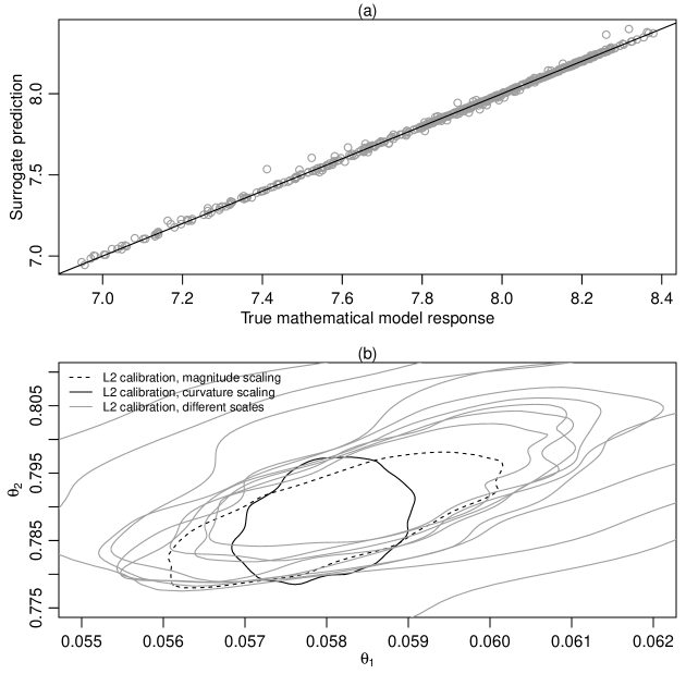
Figure SM7: Results from the radiative shock hydrodynamics example. (a) shows a plot of surrogate predictions against true mathematical model response for the 500 points in the test design. (b) shows a plot of the 50% contour of the generalized posterior for general Bayesian calibration under the $L^{2}$ loss for (i) magnitude scaling, (ii) curvature scaling (both as described in Section 3), and (iii) magnitude scaling with $\gamma=200,400,\dots,1800$ (noting that automatic magnitude scaling has $\gamma^{*}_{L^{2}}=1935$).

Figure SM8: Results from the radiative shock hydrodynamics example. The design points of the physical experiment.

SM4.2 Wiffle balls

The following example is described in Gramacy (2020, Section 8.1.2). The experiment measured the time ($y$ in seconds) for a wiffle ball to freefall a height (in the range $[0.175,4.275]$ in metres, on the original scale). There are 3 replications at each of 21 different heights giving $n=63$. Figure SM9(a) shows a plot of the observed response, $y$, against height.

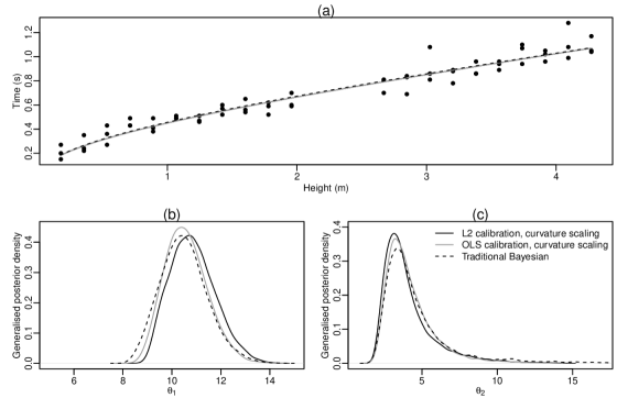
Figure SM9: Results for the wiffle ball example. Panel (a) shows a plot of time against height. The lower panels show the generalized posterior densities of $\theta_{1}$ (b) and $\theta_{2}$ (c) for general Bayesian calibration under the $L^{2}$ and OLS losses with curvature scaling and traditional Bayesian calibration. Panel (a) also shows a plot of $\eta(x,\boldsymbol{\theta})$ plotted against $x$ where $\boldsymbol{\theta}$ is the posterior mean from these three calibration methods.

The mathematical model is derived incorporating non-linear air resistance (where the force due to air resistance is proportional to the square of the wiffle ball velocity) and is given by

$$\eta(x,\boldsymbol{\theta})=\sqrt{\frac{\theta_{2}}{\theta_{1}}}\mathrm{arccosh}\left[\exp\left(\frac{x_{2}}{\theta_{2}}\right)\right].$$

The parameter $\theta_{1}$ is nominally the acceleration due to gravity and $\theta_{2}$ is related to the air resistance and mass of the wiffle balls. The prior distribution for $\boldsymbol{\theta}_{L^{2}}$ is such that the elements are independent with $\theta_{L^{2},1}\sim\mathrm{U}[0,20]$ and $\theta_{L^{2},2}\sim\mathrm{U}[0,20]$.

Table SM3 shows the posterior mean and standard deviation for $\theta_{1}$ and $\theta_{2}$ for each of the five methods. As experienced in the previous examples, there is limited difference between magnitude and curvature scaling.

Figures SM9(b) and (c) show plots of the posterior densities of $\theta_{1}$ and $\theta_{2}$, respectively, for general Bayesian calibration under the $L^{2}$ and OLS loss functions with curvature scaling (magnitude scaling omitted for clarity), and traditional Bayesian calibration.

There is very strong agreement across the different calibration methods. In particular, there is no posterior variance inflation for traditional Bayesian calibration. Consider the estimates of $L_{L^{2}}(\boldsymbol{\theta}_{L^{2}})$ and $\sigma^{2}$ given by $\ell_{L^{2}}(\hat{\boldsymbol{\theta}}_{L^{2}};\mathbf{y})=4.013\times 10^{-4}$ and $\hat{\sigma}^{2}=4.726\times 10^{-3}$, respectively. Since $\sigma^{2}$ is estimated to be an order of magnitude greater than $L_{L^{2}}(\boldsymbol{\theta}_{L^{2}})$, it explains the lack of posterior variance inflation for the traditional Bayesian posterior distribution.

	$L^{2}$	$L^{2}$	OLS	OLS	Traditional
	magnitude	curvature	magnitude	curvature	Bayesian
$\theta_{1}$	10.9	10.9	10.6	10.6	10.5
	(0.926)	(0.916)	(0.860)	(0.860)	(0.946)
$\theta_{2}$	4.06	4.10	4.19	4.19	4.57
	(1.76)	(1.77)	(1.62)	(1.62)	(2.35)

Table SM3: Results for the wiffle ball example. Generalized posterior mean (standard deviation) for $\theta_{1}$ and $\theta_{2}$ for the five different calibration methods.

References

- Ba and Joseph (2018) Ba, S. and Joseph, V. R. (2018) MaxPro: Maximum Projection Designs. URL https://CRAN.R-project.org/package=MaxPro. R package version 4.1-2.
- Billingsley (1995) Billingsley, P. (1995) Probability and Measure. New York: John Wiley and Sons 3 edn.
- Bissiri et al. (2016) Bissiri, P., Holmes, C. and Walker, S. (2016) A general framework for updating belief distributions. J. R. Stat. Soc. B 78, 1103–1130.
- Chaloner and Verdinelli (1995) Chaloner, K. and Verdinelli, K. (1995) Bayesian experimental design: a review. Stat. Sci. 10, 273–304.
- Georgiev (1988) Georgiev, A. A. (1988) Consistent nonparametric multiple regression: The fixed design case. J. Multivar. Anal. 25, 100–110.
- Gilmour and Trinca (2012) Gilmour, S. and Trinca, L. (2012) Optimum design of experiments for statistical inference (with discussion). J. R. Stat. Soc. C 61, 345–401.
- Gramacy (2020) Gramacy, R. B. (2020) Surrogates: Gaussian Process Modeling, Design and Optimization for the Applied Sciences. Boca Raton, Florida: Chapman Hall/CRC.
- Gu and Wang (2018) Gu, M. and Wang, L. (2018) Scaled Gaussian stochastic process for computer model calibration and prediction. SIAM-ASA J. Uncertain. Quantif. 6, 1555–1583.
- Jewson and Rossell (2021) Jewson, J. and Rossell, D. (2021) General Bayesian loss function selection and the use of improper models. arXiv:2106.01214.
- Joseph et al. (2015) Joseph, V., Gul, E. and Ba, S. (2015) Maximum projection designs for computer experiments. Biometrika 102, 371–380.
- Kennedy and O’Hagan (2001) Kennedy, M. and O’Hagan, A. (2001) Bayesian calibration of computer models (with discussion). J. R. Stat. Soc. B 63, 425–464.
- Lange (2010) Lange, K. (2010) Numerical Analysis for Statisticians. Springer-Verlag, New York 2nd edn.
- Miller (2021) Miller, J. (2021) Asymptotic normality, concentration, and coverage of generalized posteriors. J. Mach. Learn. Res. 22, 1–53.
- O’Hagan and Forster (2004) O’Hagan, A. and Forster, J. (2004) Kendall’s Advanced Theory of Statistics Volume 2B Bayesian Inference. Wiley 2nd edn.
- Plumlee (2017) Plumlee, M. (2017) Bayesian calibration of inexact computer models. J. Am. Stat. Assoc. 112, 1274–1285.
- Ribatet et al. (2012) Ribatet, M., Cooley, D. and Davison, A. (2012) Bayesian inference from composite likelihoods with an application to spatial extremes. Stat. Sin. 22, 813–845.
- Roberts and Rosenthal (2001) Roberts, G. and Rosenthal, J. (2001) Optimal scaling of various Metropolis-Hastings algorithms. Stat. Sci. 16, 351–367.
- Tuo and Wu (2015) Tuo, R. and Wu, C. (2015) Efficient calibration for imperfect computer models. Ann. Stat. 43, 2331–2352.
- Tuo and Wu (2016) — (2016) A theoretical framework for calibration in computer models: Parametrization, estimation and convergence properties. SIAM-ASA J. Uncertain. Quantif. 4, 767–795.
- Wilkes (1932) Wilkes, S. (1932) Certain generalizations in the analysis of variance. Biometrika 24, 471–494.
- Wong et al. (2017) Wong, R., Storlie, C. and Lee, T. (2017) A frequentist approach to computer model calibration. J. R. Stat. Soc. B 79, 635–648.
- Woody et al. (2019) Woody, S., Ghaffari, N. and Hund, L. (2019) Bayesian model calibration for extrapolative prediction via Gibbs posteriors. arXiv:1909.05428v1.
- Xie and Xu (2021) Xie, F. and Xu, Y. (2021) Bayesian projected calibration of computer models. J. Am. Stat. Assoc. 536, 1965–1982.