Composable Generative Models

Abstract

Generative modeling has recently seen many exciting developments with the advent of deep generative architectures such as Variational Auto-Encoders (VAE) or Generative Adversarial Networks (GAN). The ability to draw synthetic i.i.d. observations with the same joint probability distribution as a given dataset has a wide range of applications including representation learning, compression or imputation. It appears that it also has many applications in privacy preserving data analysis, especially when used in conjunction with differential privacy techniques.

This paper focuses on synthetic data generation models with privacy preserving applications in mind. It introduces a novel architecture, the Composable Generative Model (CGM) that is state-of-the-art in tabular data generation. Any conditional generative model can be used as a sub-component of the CGM, including CGMs themselves, allowing the generation of numerical, categorical data as well as images, text, or time series.

The CGM has been evaluated on 13 datasets (6 standard datasets and 7 simulated) and compared to 14 recent generative models. It beats the state of the art in tabular data generation by a significant margin.

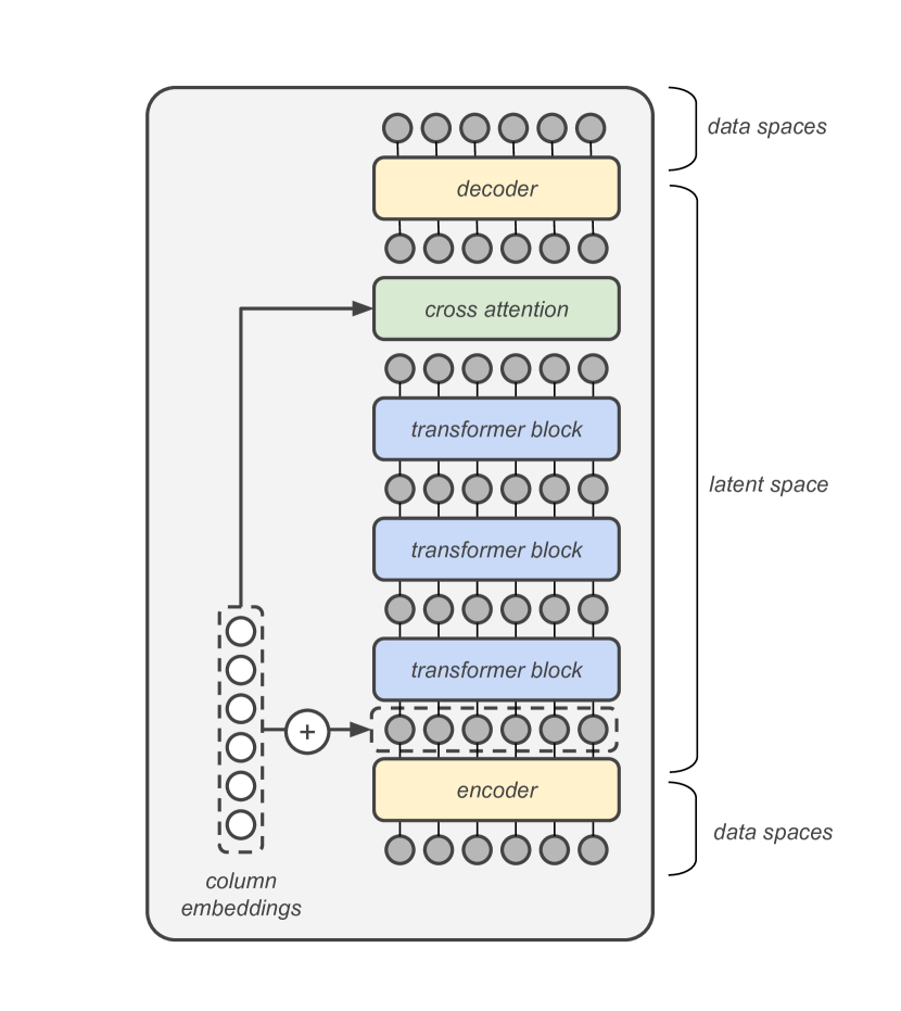
(a) Model overview

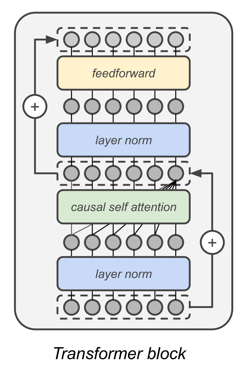
(b) Transformer block detail

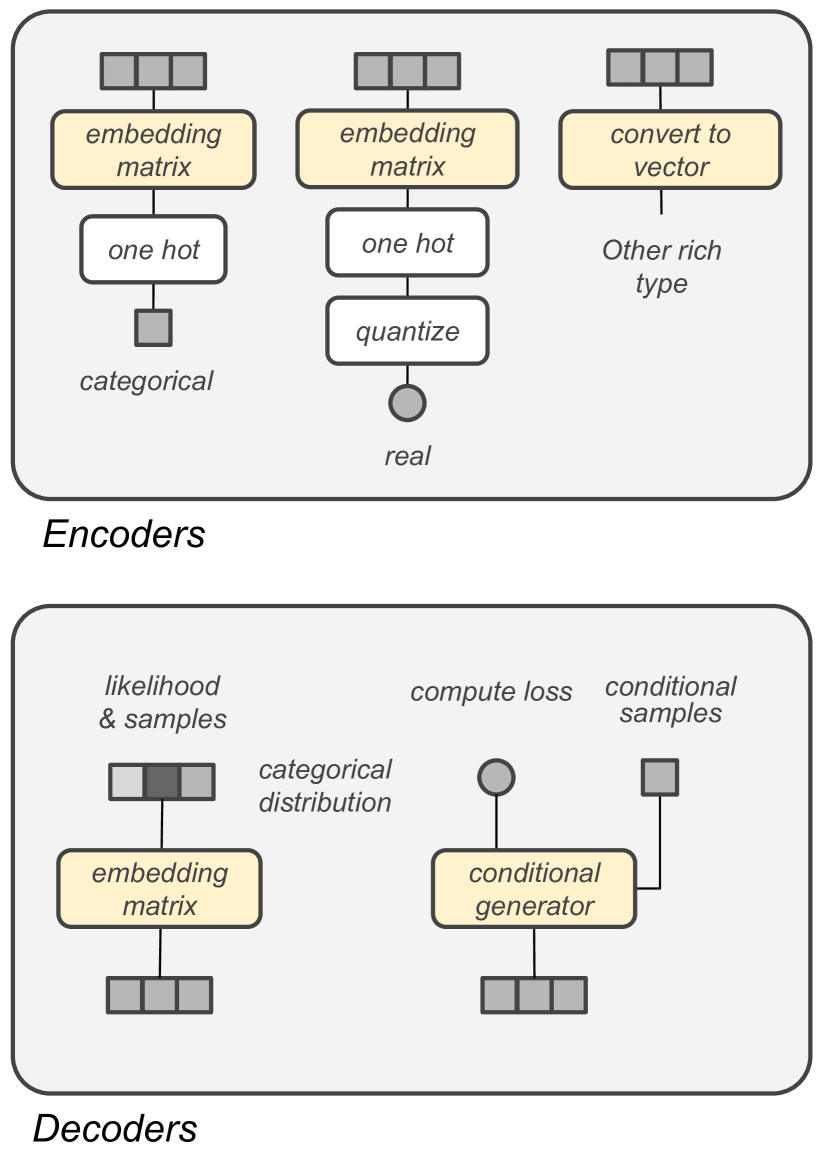
(c) Encoder and decoder detail

Figure 1: Overview of the model architecture.

1 Introduction

There have recently been impressive advances in deep generative modeling techniques, which have made new industrial applications possible.

These include new ways of collaborating on sensitive data with strong privacy guarantees such as the release of synthetic microdata by the US Census Bureau [BST⁺18]. The idea behind this application of synthetic data, is that training a generative model with differential privacy [ACG⁺16, JYVDS18], and then sharing the data generated from the model, enables the sharing of statistical properties of privacy-sensitive data, without sharing the data itself.

There is a long line of work about differential privacy [DMNS06, DR⁺14], which establishes it as a solid notion of privacy. This paper will not develop this aspect, but rather focus on generative modelling in this particular context.

A very common use-case for generating synthetic data, is the need to share privacy sensitive tabular data mixing together various column types such as numerical, categorical, or richer types like sequences or images.

Furthermore, in training a model with differentially private techniques such as DP-SGD [ACG⁺16], one generally wants to interact as little as possible with the private data to minimize privacy loss, and therefore one wants to pre-train the model with public datasets. In practice, these public datasets often have partially overlapping sets of features. To be pretrained on many of these heterogenous datasets, a synthetic data model needs to handle properly missing-data in a way similar to semi-supervised learning [KRMW14].

This paper proposes a novel deep generative model architecture (see figure 1), the Composable Generative Model (CGM), meeting the requirements specific to practical privacy preserving synthetic data generation, namely:

• to accomodate a variety of column types, continuous, discrete and potentially richer types by composing them

• to handle missing data properly

• to show good performances in modelling the joint distribution of data

The proposed architecture is autoregressive in the sense that each feature of the data is generated sequentially conditional on the features already generated. The order in which features are generated does not mater.

During training, the features are shuffled and each of them is encoded in a separate input representation vector to effectively bypass the bottleneck of encoding a variable length input into a fixed size vector [CCB15].

The input representations are then combined with column embeddings and passed through a causal transformer [VSP⁺17] that builds a set of higher level representations in a potentially generalized many-to-many cross-feature inference.

An output representation of a feature is built from the input representations of one or several other features and the embedding of the generated feature. The output representation for a feature sums up the shared knowledge of one or more other features. It is fed to a conditional generative model specialized for this feature (e.g. CNNs for images, RNNs for sequences, etc). These conditional generative models can be off-the-shelf pre-trained modules plugged into our framework. An overview of the framework is pictured on figure 1.

This work provides the following contributions:

• We describe a novel architecture built upon the Transformer, using column embeddings to encode the feature position and shuffling features during training to learn all possible combinations of missing values.

• Following [XSCIV19], we evaluate our architecture on 13 datasets (6 standard datasets and 7 simulated), compare it to 14 other generative models and demonstrate it beats the state of the art in tabular data generation

• We specify a set of requirements any conditional generative model needs to implement to be used as a component of the CGM, enabling the use of richer datatypes than numerical or categorical.

2 Related Work

2.1 Tabular data generation

Tabular data are very widespread in the industry. Yet relatively few data generation research focuses on tabular data. Traditional models for tabular data generations use decision trees, bayesian networks or copulas to sample from a data distribution.

Recent approaches have used GANs to generate tabular data. Some of them have focused their efforts on generating Electronic Health Records (EHR). MedGAN [CBM⁺17] pretrains an autoencoder and then uses the decoder as the final part of the generator, tableGAN [PMG⁺18] introduces convolutions in the generator, PATE-GAN [JYVDS18] uses the PATE framework to generate differentially private synthetic data while CTGAN and TVAE [XSCIV19] introduce a node specific normalization and conditional sampling to tackle mode collapse. The last paper also introduced a useful benchmark framework called SDGym for comparing tabular data generative models.

2.2 Composable generative models

Beyond the focus on tabular data, we designed our architecture so that it could be trained on any subset of features without having to train an exponential number of models (one for each possible subset).

Some early attempts in this direction were based on Restricted Boltzmann Machines (RBM) [SS14].

An important line of work is based on the variational auto-encoder (VAE). Composable VAEs aim to provide a flexible mechanism to compose generative models and adapt to arbitrary missing values patterns without having to learn an exponential number of mapping networks. MVAE [WG18], MMVAE [SNPT19], mmJSD [SDV20] and MHVAE [VMP20] propose to have one specialized encoder per modality (called expert) and a rule for combining the experts’ outputs together to infer the latent variable.

Our proposed approach leverages the Transformer architecture to combine several conditional generator sub-models.

2.3 Transformers

The Transformer [VSP⁺17] has been shown to excel in several modalities such as natural language [DCLT18, RWC⁺19, BMR⁺20], image [PVU⁺18, DBK⁺20] or music [HVU⁺18]. As each self-attention layer has a global receptive field, the network can give more importance to the input regions most useful for predicting a given point. Thus the architecture may be more flexible at generating diverse data types than networks with fixed connectivity patterns [CGRS19].

At the core of the Transformer is the attention operation which can be seen as a list of queries on a set of key and value pairs. We say that the attention is causal if the $k$th representation vector depends only on the $k-1$ first values. Considering a sequence of length $l$, a (key, query) dimension $d_{k}$ and a value dimension $d_{v}$, we can define the attention and causal attention operations as follows:

$$\begin{split}\text{attention}(Q,K,V)&=\text{softmax}\left(\frac{QK^{T}}{\sqrt{d_{k}}}\right)V^{T}\\ \text{causal\_attention}(Q,K,V)&=\text{softmax}\left(\frac{QK^{T}}{\sqrt{d_{k}}}-M\right)V^{T}\end{split}$$ (1)

Where $Q$ and $K$ have shape $(l,d_{k})$, $V$ has shape $(l,d_{v})$ and where the mask $M$ is a lower triangular matrix with shape $(l,l)$ where $M_{ij}=1_{j\leq i}\infty$, which enforces the causality by setting contributions of input $j$ to output $i$ to $0$ if $j>i$.

Following [VSP⁺17, RWC⁺19, BMR⁺20], we will name self-attention (or causal-self-attention) the use of a multi-head attention (or causal-attention) operation with linear transformations of the same vector passed as $Q$, $K$ and $V$ arguments.

And we will name cross-attention (or causal-cross-attention) the use of a multi-head attention (or causal-attention) operation with linear transformations of the same vector passed as $K$ and $V$ arguments and linear transformations of another vector as $Q$.

3 The Composable Generative Model

3.1 Model definition

Let us consider a tabular dataset consisting of categorical and real values. Cells can also contain missing values. In all this section, we will encode real values as categorical variables by quantizing it using its quantiles. We could also use mode aware encoding techniques as described in [XSCIV19].

Formally, we define our dataset $\mathcal{D}$ as a set of $n$ features (or columns) $\mathcal{F}_{k}$ where the $k$th feature is $d_{k}$ dimensional i.e. $\mathcal{F}_{k}\in\mathbb{R}^{d_{k}}$. The i$th$ training example consists of values $\mathcal{F}^{i}=\{f_{1}^{i},...,f_{n}^{i}\}$. Assuming training examples are i.i.d. realization of a random variable with distribution $\mathcal{F}^{i}\sim\mathcal{P_{D}}$, our objective is to train a model that can sample from an estimator $\mathcal{\hat{P}_{D}}$ maximizing the likelihood of the data.

We introduce an architecture built around a Transformer stack. We use the same transformer stack architecture as GPT-2 and GPT-3 [RWC⁺19, BMR⁺20]. The Transformer builds a sequence of representations from the input values.

For a training example $i$ and feature $k$, our model is formally defined by

$$\begin{split}\mathcal{R}^{i}&=\text{causal\_transformer}(E(\mathcal{F}^{i})+\mathcal{X})\\ y_{k}^{i}&=\text{cross\_attention}(Q=x_{k}^{i},(K,V)=\mathcal{R}_{<k}^{i})\end{split}$$ (2)

Since each feature $f_{k}^{i}$ has a priori a different dimension (i.e. number of categories), we first need to project the values to a common latent subspace so that they can then be fed into the transformer (in the same way as words are represented as dense vector embeddings). For this purpose, each feature $\mathcal{F}_{k}$ has an encoder $E_{k}$ that converts its data space to the latent space $E_{k}\left(f_{k}^{i}\right)\in\mathbb{R}^{h}$.

Furthermore, as there is no natural ordering of features, for each feature $\mathcal{F}_{k}$ we learn a column embedding $x_{k}\in\mathbb{R}^{h}$ that is integrated to the input by adding it to the latent value. The column embedding can be thought of as an origin point of the feature in the latent space $\{E_{1}(f_{1}^{i})+x_{1},...,E_{n}(f_{n}^{i})+x_{n}\}=E(\mathcal{F}^{i})+\mathcal{X}$. The column embedding is learned and identifies the columns.

The causal-Transformer is composed of a causal-self-attention operation and a position-wise feedforward network both preceded by a normalization layer and followed by a residual connection. The feedforward network has the following structure where, if $X\in\mathbb{R}^{d}$, $W_{1}$ has shape $(4d,d)$ and $W_{2}$ has shape $(d,4d)$:

$$\begin{split}\text{feedforward}(X)=W_{2}.\text{gelu}(W_{1}.X)\end{split}$$ (3)

3.2 Conditional distribution

At the output of the Transformer, the representation vector $y_{k}$ summarizes the distribution of the $k^{th}$ feature conditionally on the previous features:

$$\mathcal{P}(f_{k}|f_{1},...,f_{k-1})=\mathcal{P}(f_{k}|y_{k})$$ (4)

For each feature, we add a decoder $D_{k}$ that could be any off-the-shelf conditional generation model and trained accordingly. The decoder $D_{k}$ allows us to compare the conditional distribution to the expected data distribution. The provided error signal for each feature is backpropagated to train the whole model.

In this paper, we only consider the case of the conditional categorical generative model. For this purpose, we reuse the embedding matrix $E_{k}$ used to transform the one-hot encoded vectors to dense latent vactor. We multiply the conditional vector $y_{k}\in\mathbb{R}^{h}$ with the transpose of the embedding matrix $E_{k}\in\mathbb{R}^{(h,d_{k})}$ to produce an $n_{k}$ dimentional vector representing the logits of the categorical distribution $\mathcal{P}(f_{k}|y_{k})$, where $d_{k}$ is the number of caterogies (or quantiles) of the $k^{th}$ feature.

$$\mathcal{P}(f_{k}|y_{k})=\text{softmax}(E_{k}^{T}y_{k})$$ (5)

The model then minimize the loss $\mathcal{L}$ which is the categorical cross-entropy accross all columns as written in equation 6 where $f_{k}$ is a one-hot encoded vector.

$$\mathcal{L}=-\sum_{k}f_{k}\log(\text{softmax}(E_{k}^{T}y_{k}))$$ (6)

3.3 Training CGMs

Feature order

One of the advantages of this model compared to a traditional architecture [UCG⁺16] is the fact that the autoregressive order does not need to be fixed. For each training example, a random permutation of the input features is chosen and the probability distribution of the $k^{th}$ feature conditionally on a random subset of the remaining features is computed. The training algorithm is summarized in algorithm 1.

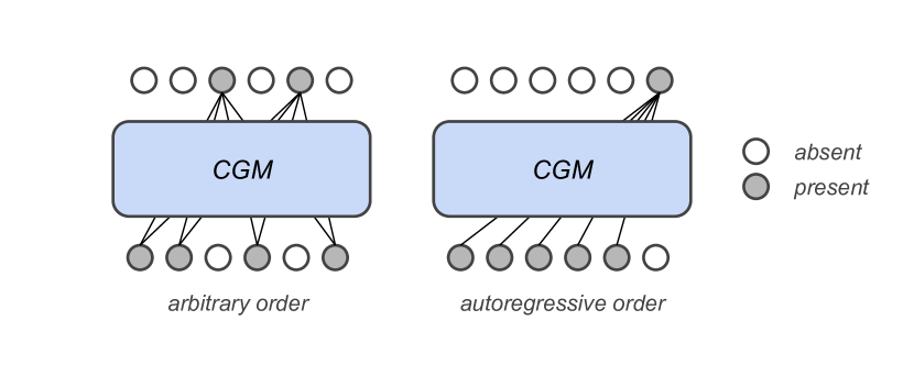
Figure 2: CGM can use any set of columns to make predictions.

Weakly-supervised setting

Another advantage of our model is its ability to be trained in a weakly-supervised setting, that is, when some columns have missing values. This is possible since the columns are referred to by explicitly learned column embedding as shown in figure 2.

Initialize $\theta_{E},\theta_{T},\theta_{D}$;

while not converged do

       $\mathcal{H}\leftarrow E(\mathcal{F})+\mathcal{X}$;

       $\mathcal{H}\leftarrow\text{permute}(\mathcal{H})$;

       $\mathcal{R}\leftarrow\text{causal\_transformer}(\mathcal{H})$;

       $y_{k}\leftarrow\text{cross\_attention}(Q=x_{k},(K,V)=\mathcal{R}_{<k}),\forall k$;

       $\mathcal{L}\leftarrow-\sum_{k}f_{k}\log(\text{softmax}(E_{k}^{T}y_{k}))$;

       $\theta_{E},\theta_{T},\theta_{D}\leftarrow(\theta_{E},\theta_{T},\theta_{D})-\lambda\nabla_{\theta_{D},\theta_{T},\theta_{D}}\mathcal{L}$;

end while

Algorithm 1 Training algorithm

3.4 Generation with CGMs

Once trained, the model can be used for generation. The first representation vector is generated using an empty set of features. The first features is then sampled from the representation. The other features are generated conditionally on the ones already generated:

$$\begin{split}\mathcal{R}&=\text{causal\_transformer}(E(\mathcal{F})+\mathcal{X})\\ y_{k}&=\text{cross\_attention}(Q=x_{k},(K,V)=\mathcal{R}_{<k})\\ f_{k}&\sim\mathcal{P}(f_{k}|y_{k})\end{split}$$ (7)

4 Composing a model with richer types

Because it is trained with feature shuffling, it is possible to remove or add features to the CGM at any stage of the training. Those features can be numerical or categorical as described above, but they could be of a richer type provided the type implements the interface specified below:

Encoder

the type of feature $\mathcal{F}_{k}$ should be equiped with an encoder, mapping a value $f_{k}^{i}$ from the data to an input representation: $E_{k}:\to\mathbb{R}^{h}$

The encoder can be a neural network, parametrized by weights and trained along with those of the transformer.

Decoder

the type of feature $\mathcal{F}_{k}$ should be able equiped with a decoder, sampling a value $f_{k}\in\mathbb{R}^{d_{k}}$ from an output representation $y_{k}in\mathbb{R}^{h}$: $f_{k}\sim\mathcal{P}(f_{k}|y_{k})$

The decoder can be a neural network, parametrized by weights and trained along with those of the transformer.

Loss

the type of feature $\mathcal{F}_{k}$ should provide the loss to minimize during training of the weights of the transformer along with encoder weights and decoder weights.

The loss can also be parametrized as a neural network and trained against an adversarial loss, thus permiting the integration of Generative Adversarial Networks [GPAM⁺14] as the decoder part of a rich type (like images or sound).

When considering a categorical feature, the encoder is simply parametrized by an embedding matrix giving the input representation vector corresponding to the $i^{th}$ modality by a simple look-up operation. The decoder is also parametrized by an embedding matrix converting an output representation vector to a vectors of logits fed into a softmax. Then a value is sampled from the probabilities derived from the softmax. The loss is simply the categorical cross-entropy.

Numerical feature are converted to categorical by quantization. The encoder and decoder have the same form as those of a categorical feature, simply composed with a quantization, de-quantization step.

If one wants to produce synthetic data with columns of images, one can simply implement the specifications above. The encoder can be a deep convolutional network, the decoder the generator network of a GAN and the loss the dicriminator network of the GAN. In that case two adversarial objectives are optimized during training, the minimization of the common loss of all the encoders, decoders and transformer networks, and the minimization of the adversarial loss of the discriminators of image features.

Beyond images, one can integrate sequences usng RNN or Transformers, NLP and more. The setting with images categorical and numerical features has been tested and works fine. And further types are being integrated in the model.

5 Application to tabular data

In this section we present the experiments we conducted to test the performance and applications of our model on tabular data.

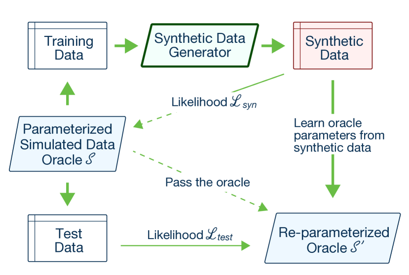
(a) SDGym process for synthetic datasets.

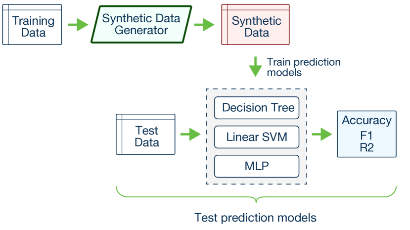
(b) SDGym process for real datasets.

Figure 3: Overview of the SDGym scoring process [XSCIV19].

	adult		census		covtype		credit		intrusion
	acc	f1	acc	f1	acc	f1	acc	f1	acc	f1
Uniform	0.49	0.24	0.54	0.11	0.14	0.09	0.57	0.01	0.12	0.07
Independent	0.64	0.15	0.66	0.06	0.38	0.11	0.88	0.00	0.72	0.20
GCCF	0.77	0.26	0.79	0.05	0.42	0.14	0.98	0.01	0.84	0.26
GCOH	0.78	0.20	0.93	0.13	0.51	0.18	1.00	0.00	0.90	0.33
CopulaGAN	0.79	0.61	0.89	0.39	0.57	0.33	1.00	0.72	0.98	0.52
CLBN	0.77	0.31	0.90	0.29	0.56	0.33	1.00	0.44	0.94	0.39
PrivBN	0.80	0.43	0.90	0.24	0.47	0.21	0.96	0.01	0.95	0.38
Medgan	0.62	0.24	0.64	0.14	0.44	0.09	0.94	0.02	0.87	0.27
VEEGAN	0.72	0.16	0.76	0.05	0.22	0.10	0.88	0.17	0.51	0.18
TVAE	0.80	0.62	0.93	0.38	0.65	0.46	1.00	0.00	0.97	0.43
CTGAN	0.80	0.60	0.90	0.38	0.58	0.33	0.99	0.52	0.98	0.51
CGM(ours)	0.83	0.65	0.91	0.41	0.70	0.49	1.00	0.53	0.99	0.59
Identity	0.82	0.66	0.91	0.46	0.76	0.65	0.99	0.55	1.00	0.86

Figure 4: Real datasets leaderboard. Each synthesizer is trained on a training split $\mathcal{T}_{train}$ of the real data. Synthetic data $\mathcal{T}_{syn}$ are generated and a classifier is trained on it. The classifier’s accuracy and f1-score are then measured on a test split $\mathcal{T}_{test}$ of the real data.

	grid		gridr		ring
	$\mathcal{L}_{syn}$	$\mathcal{L}_{test}$	$\mathcal{L}_{syn}$	$\mathcal{L}_{test}$	$\mathcal{L}_{syn}$	$\mathcal{L}_{test}$
Uniform	-7.33	-4.54	-7.22	-4.57	-5.34	-2.50
Independent	-3.47	-3.49	-5.12	-4.03	-2.47	-1.96
GCC	-7.24	-4.51	-7.16	-4.54	-3.20	-2.15
GCCF	-7.34	-4.57	-7.14	-4.55	-3.18	-2.15
GCOH	-7.27	-4.51	-7.19	-4.55	-3.21	-2.15
CopulaGAN	-8.19	-5.14	-8.16	-5.01	-6.21	-2.80
CLBN	-3.88	-9.20	-4.01	-7.43	-1.77	-47.16
Medgan	-5.83	-90.34	-7.37	-141.41	-2.78	-149.77
VEEGAN	-8.65	-423.57	-11.46	-8.91	-16.83	-6.35
Tablegan	-6.99	-5.33	-7.00	-4.83	-4.74	-2.53
TVAE	-3.27	-5.66	-3.87	-3.71	-1.58	-1.94
CTGAN	-8.92	-5.09	-8.32	-5.03	-7.13	-2.70
CGM(ours)	-3.50	-3.54	-3.89	-3.71	-1.82	-1.74
Identity	-3.47	-3.49	-3.59	-3.64	-1.71	-1.70

Figure 5: Synthetic datasets leaderboard. A parametric model $\mathcal{M}$ is used to generate training data $\mathcal{T}_{train}$ and test data $\mathcal{T}_{test}$. Each synthesizer is trained and generates synthetic data $\mathcal{T}_{syn}$. The log-likelihood of the synthetic data wrt. $\mathcal{M}$ is computed $\mathcal{L}_{syn}=log(P(\mathcal{T}_{syn}|\mathcal{M}))$. The parametric model is also refitted using $\mathcal{T}_{syn}$ and yield a new model $\mathcal{M}^{\prime}$. The log-likelihood of the test data wrt. $\mathcal{M}^{\prime}$ is computed $\mathcal{L}_{test}=log(P(\mathcal{T}_{test}|\mathcal{M}^{\prime}))$.

	alarm		asia		child		insurance
	$\mathcal{L}_{syn}$	$\mathcal{L}_{test}$	$\mathcal{L}_{syn}$	$\mathcal{L}_{test}$	$\mathcal{L}_{syn}$	$\mathcal{L}_{test}$	$\mathcal{L}_{syn}$	$\mathcal{L}_{test}$
Uniform	-18.42	-18.42	-14.28	-5.52	-18.41	-18.32	-18.42	-18.42
Independent	-18.24	-15.82	-4.97	-2.99	-17.96	-16.03	-18.38	-17.57
GCC	-12.91	-15.57	-2.25	-3.61	-16.40	-15.55	-17.84	-16.58
GCCF	-14.52	-14.57	-2.83	-3.11	-16.90	-15.41	-18.03	-16.52
GCOH	-15.48	-15.67	-2.31	-3.23	-14.48	-15.31	-17.84	-17.91
CopulaGAN	-15.69	-13.05	-3.96	-2.40	-14.25	-12.92	-16.96	-14.96
CLBN	-12.46	-11.19	-2.40	-2.27	-12.63	-12.31	-15.17	-13.92
PrivBN	-12.15	-11.14	-2.29	-2.24	-12.36	-12.19	-14.70	-13.64
Medgan	-7.84	-13.26	-1.57	-5.97	-11.11	-12.99	-13.88	-15.08
VEEGAN	-18.39	-18.21	-11.49	-5.95	-17.31	-17.68	-18.33	-18.11
Tablegan	-12.69	-11.54	-3.40	-2.72	-15.02	-13.39	-16.18	-14.32
TVAE	-11.44	-10.76	-2.29	-2.27	-12.46	-12.30	-14.30	-14.24
CTGAN	-15.22	-12.93	-2.69	-2.31	-13.81	-12.81	-16.60	-14.84
CGM(ours)	-10.63	-10.48	-2.33	-2.25	-11.83	-12.13	-13.21	-13.11
Identity	-10.23	-10.30	-2.24	-2.24	-12.03	-12.04	-12.85	-12.96

Figure 6: Bayesian datasets leaderboard. A parametric model $\mathcal{M}$ is used to generate training data $\mathcal{T}_{train}$ and test data $\mathcal{T}_{test}$. Each synthesizer is trained and generates synthetic data $\mathcal{T}_{syn}$. The log-likelihood of the synthetic data wrt. $\mathcal{M}$ is computed $\mathcal{L}_{syn}=log(P(\mathcal{T}_{syn}|\mathcal{M}))$. The parametric model is also refitted using $\mathcal{T}_{syn}$ and yield a new model $\mathcal{M}^{\prime}$. The log-likelihood of the test data wrt. $\mathcal{M}^{\prime}$ is computed $\mathcal{L}_{test}=log(P(\mathcal{T}_{test}|\mathcal{M}^{\prime}))$.

We trained the model on tabular data and benchmarked against the SDGym leaderboard. SDGym evaluates the performance of synthetic data generators on three dataset families: simulated data using gaussian mixtures, simulated data using bayesian networks and real world datasets [XSCIV19].

We evaluated our model using the publicly available SDGym benchmark [XSCIV19]. The model’s performance at generating synthetic data is measured against several other models on different types of datasets.

The test procedure is different for datasets generated with a parametric model $\mathcal{M}$ (synthetic and bayesian) and real datasets as seen on figure 3. For each dataset, the data is split into a training set $\mathcal{T}_{train}$ and a test set $\mathcal{T}_{test}$. The generative model is trained on $\mathcal{T}_{train}$ and a synthetic data set $\mathcal{T}_{syn}$ is generated.

Synthetic and bayesian datasets

For generated datasets (synthetic and bayesian datasets), the probability distribution of the data is known. We can thus evaluate the log-likelihood of the synthetized data with respect to the parametric model $\mathcal{M}$ that is $\mathcal{L}_{syn}=log(P(\mathcal{T}_{syn}|\mathcal{M}))$. However, such a metric favors mode collapsed models. To measure if mode collapse has occured, the parametric model $\mathcal{M}$ that was used to generate $\mathcal{T}_{train}$ is refitted using $\mathcal{T}_{syn}$ instead. This yields a new parametric model $\mathcal{M}^{\prime}$. The log-likelihood of the test set $\mathcal{T}_{test}$ with respect to $\mathcal{M}^{\prime}$ is then computed $\mathcal{L}_{test}=log(P(\mathcal{T}_{test}|\mathcal{M}^{\prime}))$.

Real datasets

For real datasets, the machine learning efficacy is used to measure the quality of the synthetic data. A classification model is trained using $\mathcal{T}_{syn}$ and the accuracy $acc$ and $f1$ scores are measured on the test set $\mathcal{T}_{test}$.

For all datasets, we used a hidden dimension of 64 and a transformer composed of 2 blocks with 8 heads. We trained the generative model for 15 epochs with a batch size of $128$ and the Adam optimizer with $\beta_{1}=0.5$, $\beta_{2}=0.99$, a learning rate of $0.001$. All computations were done on a machine with 8 CPUs and 2 NVIDIA V100 GPUs. Benchmarking on all SDGym datasets took 4 hours.

5.1 Results

We compare our results with the public leaderboard provided on the SDGym web page. The scores of several models have been pre-computed for comparison. We are compared against the following models: GCC (Gaussian Copula Categorical), GCCF (Gaussian Copula Categorical Fuzzy), GCOH (Gaussian Copula One Hot), CopulaGAN, CLBN, PrivBN, Medgan, Tablegan, CTGAN and TVAE.

Trivial synthesizers are also benchmarked: the Uniform synthesizer generates data uniformly and serves as a lower bound likelihood estimator, the Independent synthesizer makes an independence assumption and the Identity synthesizer simply returns the training data and serves as a likelihood upper bound estimator. The actual scores are presented on figures 4, 5 and 6.

For model comparison, we will focus on the $\mathcal{L}_{test}$ and f1-scores since the other metrics (accuracy and $\mathcal{L}_{syn}$) do not reflect the synthetic data quality as good. To easily visualize the results, we put in bold the best result in each column.

As we can see, our model outperforms the other models on the real datasets. On the credit dataset, we can see that the CopulaGAN model outperforms us but that is also outperforms the Identity synthesizer by a large margin. Such a high performance, better than the perfect Identity synthesizer, is odd and could be attributed to the fact that the synthesized data are better suited to train the subsequent classifier whereas the real data may contain outliers that perturb the classifier’s training process.

On synthetic datasets, our model is the leader in the outperformed gridr and ring datasets. It is slightly outperformed by the trivial Independent synthesizer on the grid dataset but is the second best model by a large margin.

On bayesian datasets, our model is the leader on the alarm, asia and insurance datasets. Our model is very close to the PrivBN synthesizer on the asia dataset though slightly outperformed.

6 The CGM in production

The CGM is used in production at Sarus Technologies for the generation of synthetic data.

Sarus is a technology company developing solutions to analyze privacy-sensitive data with formal privacy guarantees.

In production, the CGM is trained with DP-SGD [ACG⁺16] in order to provide differential privacy guarantees to the data generator.

The solution has been applied in medical data sharing with the French National Institute in Medical Research (INSERM) and it is being experimented in various institutions in finance, energy, and transportation.

7 Conclusion

Though we focus on categorical and numerical data in this paper, the CGM can accomodate a wide range of types.

Besides, as demonstrated, the CGM is able to be pre-trained on many public datasets before it is trained on private data.

Both those improvements and the quality of the data generated, open new possibilities in privacy preserving data analysis, enabling new applications in health care, personal finance or public policy planning.

References

- [ACG+16] Martin Abadi, Andy Chu, Ian Goodfellow, H Brendan McMahan, Ilya Mironov, Kunal Talwar, and Li Zhang. Deep learning with differential privacy. In Proceedings of the 2016 ACM SIGSAC conference on computer and communications security, pages 308–318, 2016.
- [BMR+20] Tom B Brown, Benjamin Mann, Nick Ryder, Melanie Subbiah, Jared Kaplan, Prafulla Dhariwal, Arvind Neelakantan, Pranav Shyam, Girish Sastry, Amanda Askell, et al. Language models are few-shot learners. arXiv preprint arXiv:2005.14165, 2020.
- [BST+18] Gary Benedetto, Jordan C Stanley, Evan Totty, et al. The creation and use of the sipp synthetic beta v7. 0. US Census Bureau, 2018.
- [CBM+17] Edward Choi, Siddharth Biswal, Bradley Malin, Jon Duke, Walter F Stewart, and Jimeng Sun. Generating multi-label discrete patient records using generative adversarial networks. In Machine learning for healthcare conference, pages 286–305. PMLR, 2017.
- [CCB15] Kyunghyun Cho, Aaron Courville, and Yoshua Bengio. Describing multimedia content using attention-based encoder-decoder networks. IEEE Transactions on Multimedia, 17(11):1875–1886, 2015.
- [CGRS19] Rewon Child, Scott Gray, Alec Radford, and Ilya Sutskever. Generating long sequences with sparse transformers. arXiv preprint arXiv:1904.10509, 2019.
- [DBK+20] Alexey Dosovitskiy, Lucas Beyer, Alexander Kolesnikov, Dirk Weissenborn, Xiaohua Zhai, Thomas Unterthiner, Mostafa Dehghani, Matthias Minderer, Georg Heigold, Sylvain Gelly, et al. An image is worth 16x16 words: Transformers for image recognition at scale. arXiv preprint arXiv:2010.11929, 2020.
- [DCLT18] Jacob Devlin, Ming-Wei Chang, Kenton Lee, and Kristina Toutanova. Bert: Pre-training of deep bidirectional transformers for language understanding. arXiv preprint arXiv:1810.04805, 2018.
- [DMNS06] Cynthia Dwork, Frank McSherry, Kobbi Nissim, and Adam Smith. Calibrating noise to sensitivity in private data analysis. In Theory of cryptography conference, pages 265–284. Springer, 2006.
- [DR+14] Cynthia Dwork, Aaron Roth, et al. The algorithmic foundations of differential privacy. Foundations and Trends in Theoretical Computer Science, 9(3-4):211–407, 2014.
- [GPAM+14] Ian J Goodfellow, Jean Pouget-Abadie, Mehdi Mirza, Bing Xu, David Warde-Farley, Sherjil Ozair, Aaron Courville, and Yoshua Bengio. Generative adversarial nets. stat, 1050:10, 2014.
- [HVU+18] Cheng-Zhi Anna Huang, Ashish Vaswani, Jakob Uszkoreit, Noam Shazeer, Ian Simon, Curtis Hawthorne, Andrew M Dai, Matthew D Hoffman, Monica Dinculescu, and Douglas Eck. Music transformer. arXiv preprint arXiv:1809.04281, 2018.
- [JYVDS18] James Jordon, Jinsung Yoon, and Mihaela Van Der Schaar. Pate-gan: Generating synthetic data with differential privacy guarantees. In International Conference on Learning Representations, 2018.
- [KRMW14] Diederik P Kingma, Danilo J Rezende, Shakir Mohamed, and Max Welling. Semi-supervised learning with deep generative models. arXiv preprint arXiv:1406.5298, 2014.
- [PMG+18] Noseong Park, Mahmoud Mohammadi, Kshitij Gorde, Sushil Jajodia, Hongkyu Park, and Youngmin Kim. Data synthesis based on generative adversarial networks. Proc. VLDB Endow., page 1071–1083, 2018.
- [PVU+18] Niki Parmar, Ashish Vaswani, Jakob Uszkoreit, Lukasz Kaiser, Noam Shazeer, Alexander Ku, and Dustin Tran. Image transformer. In International Conference on Machine Learning, pages 4055–4064. PMLR, 2018.
- [RWC+19] Alec Radford, Jeffrey Wu, Rewon Child, David Luan, Dario Amodei, and Ilya Sutskever. Language models are unsupervised multitask learners. OpenAI blog, 1(8):9, 2019.
- [SDV20] Thomas M Sutter, Imant Daunhawer, and Julia E Vogt. Multimodal generative learning utilizing jensen-shannon-divergence. arXiv preprint arXiv:2006.08242, 2020.
- [SNPT19] Yuge Shi, Siddharth Narayanaswamy, Brooks Paige, and Philip H. S. Torr. Variational mixture-of-experts autoencoders for multi-modal deep generative models. In NIPS, 2019.
- [SS14] Nitish Srivastava and Ruslan Salakhutdinov. Multimodal learning with deep boltzmann machines. J. Mach. Learn. Res., 15(1):2949–2980, 2014.
- [UCG+16] Benigno Uria, Marc-Alexandre Côté, Karol Gregor, Iain Murray, and Hugo Larochelle. Neural autoregressive distribution estimation. The Journal of Machine Learning Research, 17(1):7184–7220, 2016.
- [VMP20] Miguel Vasco, Francisco S Melo, and Ana Paiva. Mhvae: a human-inspired deep hierarchical generative model for multimodal representation learning. arXiv preprint arXiv:2006.02991, 2020.
- [VSP+17] Ashish Vaswani, Noam Shazeer, Niki Parmar, Jakob Uszkoreit, Llion Jones, Aidan N Gomez, Lukasz Kaiser, and Illia Polosukhin. Attention is all you need. In NIPS, 2017.
- [WG18] Mike Wu and Noah Goodman. Multimodal generative models for scalable weakly-supervised learning. arXiv preprint arXiv:1802.05335, 2018.
- [XSCIV19] Lei Xu, Maria Skoularidou, Alfredo Cuesta-Infante, and Kalyan Veeramachaneni. Modeling tabular data using conditional gan. In H. Wallach, H. Larochelle, A. Beygelzimer, F. d'Alché-Buc, E. Fox, and R. Garnett, editors, Advances in Neural Information Processing Systems, volume 32, pages 7335–7345. Curran Associates, Inc., 2019.