Adaptive Step-Length Selection in Gradient Boosting for Generalized Additive Models for Location, Scale and Shape

Abstract

Tuning of model-based boosting algorithms relies mainly on the number of iterations, while the step-length is fixed at a predefined value. For complex models with several predictors such as Generalized Additive Models for Location, Scale and Shape (GAMLSS), imbalanced updates of predictors, where some distribution parameters are updated more frequently than others, can be a problem that prevents some submodels to be appropriately fitted within a limited number of boosting iterations. We propose an approach using adaptive step-length (ASL) determination within a non-cyclical boosting algorithm for GAMLSS to prevent such imbalance. Moreover, for the important special case of the Gaussian distribution, we discuss properties of the ASL and derive a semi-analytical form of the ASL that avoids manual selection of the search interval and numerical optimization to find the optimal step-length, and consequently improves computational efficiency. We show competitive behavior of the proposed approaches compared to penalized maximum likelihood and boosting with a fixed step-length for GAMLSS models in two simulations and two applications, in particular for cases of large variance and/or more variables than observations. In addition, the idea of the ASL is also applicable to other models with more than one predictor like zero-inflated count model, and brings up insights into the choice of the reasonable defaults for the step-length in simpler special case of (Gaussian) additive models.

Keywords— Step-Length, Gradient Boosting, GAMLSS, Variable Selection, Shrinkage

1 Introduction

Generalized additive models for location, scale and shape (GAMLSS)[Rigby and Stasinopoulos (2005)] are distribution-based approaches, where all parameters of the assumed distribution for the response can be modelled as additive functions of the explanatory variables [Ripley (2004); Stasinopoulos et al. (2017)]. Specifically, the GAMLSS framework allows the conditional distribution of the response variable to come from a wide variety of discrete, continuous and mixed discrete-continuous distributions, see Stasinopoulos and Rigby (2007). Unlike conventional generalized additive models (GAMs), GAMLSS not only model the location parameter, e.g. the mean for Gaussian distributions, but also further distribution parameters such as scale (variance) and shape (skewness and kurtosis) through the explanatory variables in linear, nonlinear or smooth functional form.

The coefficients of GAMLSS are usually estimated based on penalized maximum likelihood method [Rigby and Stasinopoulos (2005)]. However, this approach cannot deal with high dimensional data, or more precisely, the case of more variables than observations [Bühlmann (2006)]. As the selection of informative covariates is an important part of practical analysis, Mayr et al. (2012) combined the GAMLSS framework with componentwise gradient boosting [Bühlmann and Yu (2003); Hofner et al. (2014); Hothorn et al. (2018)] such that variable selection and estimation can be performed simultaneously. The original method cyclically updates the distribution parameters, i.e. all predictors will be updated sequentially in each boosting iteration [Hofner et al. (2016)]. Because the levels of complexity vary across the prediction functions, separate stopping values are required for each distribution parameter. Consequently, these stopping values have to be optimized jointly as they are not independent of each other. The commonly applied joint optimization methods like grid search are, however, computationally very demanding. For this reason, Thomas et al. (2018) proposed an alternative non-cyclical algorithm that updates only one distribution parameter (yielding the strongest improvement) in each boosting iteration. This way, only one global stopping value is needed and the resulting one-dimensional optimization procedure vastly reduces computing complexity for the boosting algorithm compared to the previous multi-dimensional one. The non-cyclical algorithm can be combined with stability selection [Meinshausen and Bühlmann (2010); Hofner et al. (2015)] to further reduce the selection of false positives [Hothorn et al. (2010)].

In contrast to the cyclical approach, the non-cyclical algorithm avoids an equal number of updates for all distribution parameters as it is not useful to artificially enforce updates for parameters with a less complex structure than other parameters. However, it becomes even more important to fairly select the predictor to be updated in any given iteration. The current implementation of Thomas et al. (2018), however, uses fixed and equal step-lengths for all updates, regardless of the achieved loss reduction of different distribution parameters. As we demonstrate later, this leads to imbalanced updates that affect the fair selection and predictors with large number of boosting iterations still tend to be underfitted. This seems inconsistent, since one expects the underfitted predictor to be updated with a few number of iterations. As we show later, a large $\boldsymbol{\sigma}$ in a Gaussian distribution leads to a small negative gradient of $\boldsymbol{\mu}$ and consequently the improvement for $\boldsymbol{\mu}$ with fixed small step-lengths in each boosting iteration will also be small. This results in the algorithm needing a lot of updates for $\boldsymbol{\mu}$ until its empirical risk decreases to the level of $\boldsymbol{\sigma}$. However, the algorithm may stop long before the corresponding coefficients are well estimated.

We address this problem by proposing a version of the non-cyclical boosting algorithm for GAMLSS that adaptively and automatically optimizes the step-lengths for all predictors in each boosting iteration. The new approach leads to a fair selection of predictors to update. While it does not enforce equal numbers of updates for all distribution parameters, it yields a natural balance in the updates. For the Gaussian distribution, we also derive (semi-)analytical adaptive step-lengths that decrease the need for numerical optimization and discuss their properties. Our findings have implications beyond boosted GAMLSS models for boosting other models with several predictors, e.g. for zero-inflated count models, and also give insights into the step-length choice for the simpler special case of (Gaussian) additive models.

The structure of this paper is organized as follows: Section 2 introduces the boosted GAMLSS models including the cyclical and non-cyclical algorithms. Section 3 discusses how to apply the adaptive step-length on the non-cyclical boosted GAMLSS algorithm, and introduces the semi-analytical solutions of the adaptive step-length in the Gaussian distribution with their properties. Section 4 evaluates the performance of the adaptive algorithms and the problem of fixed step-length in two simulations. Section 5 presents the application of the adaptive algorithms for two datasets: the malnutrition data, where the outcome variance is very large, and the riboflavin data, which has more variables than observations. Section 6 concludes with a summary and discussion. Further relevant materials and results are included in the appendix.

2 Boosted GAMLSS

In this section, we briefly introduce the GAMLSS models and the two cyclical and noncyclical boosting methods for estimation.

2.1 GAMLSS and componentwise gradient boosting

Conventional generalized additive models (GAM) assume a dependence only of the conditional mean $\mu$ of the response on the covariates. GAMLSS, however, also model other distribution parameters such as the scale $\sigma$, skewness $\nu$ and/or kurtosis $\tau$ with a set of statistical models.

The $K$ distribution parameters $\boldsymbol{\theta}^{T}=(\boldsymbol{\theta}_{1},\boldsymbol{\theta}_{2},\cdots,\boldsymbol{\theta}_{K})$ of a density function $f(\boldsymbol{y}|\boldsymbol{\theta})$ are modelled by a set of up to $K$ additive models. The model class assumes that the observations $y_{i}$ for $i\in\{1,\cdots,n\}$ are conditionally independent given a set of explanatory variables. Let $\boldsymbol{y}^{T}=(y_{1},y_{2},\cdots,y_{n})$ be a vector of the response variable and $\boldsymbol{X}$ be a $n\times J$ data matrix. In addition, we denote $\boldsymbol{X}_{i\cdot}$, $\boldsymbol{X}_{\cdot j}$ and $X_{ij}$ as the $i$-th observation (vector of length $J$), $j$-variable (vector of length $n$) and the $i$-th observation of the $j$-th variable (a single value) respectively. Let $g_{k}(\cdot),k=1,\cdots,K$ be known monotonic link functions that relate $K$ distribution parameters to explanatory variables through additive models given by

$$g_{k}(\boldsymbol{\theta}_{k})=\eta_{\boldsymbol{\theta}_{k}}(\boldsymbol{X})=\beta_{0,\boldsymbol{\theta}_{k}}\boldsymbol{1}_{n}+\sum_{j=1}^{J}f_{j,\boldsymbol{\theta}_{k}}(\boldsymbol{X}_{\cdot j}|\beta_{j,\boldsymbol{\theta}_{k}})\quad k=1,\dots,K,$$ (1)

where $\boldsymbol{\theta}_{k}=(\theta_{k,1},\cdots,\theta_{k,n})^{T}$ contains the $n$ parameter values for the $n$ observations and functions are applied elementwise if the argument is a vector, $\boldsymbol{\eta}_{\theta_{k}}$ is a vector of length $n$, $\boldsymbol{1}_{n}$ is a vector of ones and $\beta_{0,\boldsymbol{\theta}_{k}}$ is the model parameter specific intercept. Function $f_{j,\boldsymbol{\theta}_{k}}(\boldsymbol{X}_{\cdot j}|\beta_{j,\boldsymbol{\theta}_{k}})$ indicates the effects of the $j$-th explanatory variable $\boldsymbol{X}_{\cdot j}$ (vector of length $n$) for the model parameter $\boldsymbol{\theta}_{k}$, and $\beta_{j,\boldsymbol{\theta_{k}}}$ is the parameter of the additive predictor $f_{j,\boldsymbol{\theta}_{k}}(\cdot)$. Various types of effects (e.g., linear, smooth, random) for $f(\cdot)$ are allowed. If the location parameter $(\theta_{1}=\mu)$ is the only distribution parameter to be regressed ($K=1$) and the response variable is from the exponential family, (1) reduces to the conventional GAM. In addition, $f_{j}$ can depend on more than one variable (interaction), in which case $X_{\cdot j}$ would be e.g. a $n\times 2$ matrix, but for simplicity we ignore this case in the notation.

A penalized likelihood approach can be used to estimate the unknown quantities; for more details, see Rigby and Stasinopoulos (2005). However, this approach does not allow parameter estimation in the case of more explanatory variables than observations, and variable selection for high-dimensional data is not possible. To deal with these problems, Mayr et al. (2012) proposed a boosted GAMLSS algorithm, which estimates the predictors in GAMLSS with componentwise gradient boosting [Bühlmann and Yu (2003)]. As this method updates in general only one variable in each iteration, it can deal with data that has more variables than observations, and the important variables can be selected by controlling the stopping iterations.

To estimate the unknown predictor parameters $\beta_{j,\boldsymbol{\theta}_{k}},j\in\{1,\cdots,J\}$ in equation (1), the componentwise gradient boosting algorithm minimizes the empirical risk $R$, which is also the loss $\rho$ summed over all observations,

$$R=\sum_{i=1}^{n}\rho\left(y_{i},\boldsymbol{\eta}(\boldsymbol{X}_{i\cdot})\right),$$

where the loss $\rho$ measures the discrepancy between the response $y_{i}$ and the predictor $\boldsymbol{\eta}(\boldsymbol{X}_{i\cdot})$. The predictor $\boldsymbol{\eta}(\boldsymbol{X}_{i\cdot})=\left(\eta_{\boldsymbol{\theta}_{1}}(\boldsymbol{X}_{i\cdot}),\cdots,\eta_{\boldsymbol{\theta}_{K}}(\boldsymbol{X}_{i\cdot})\right)$ is a vector of length $K$. For the $i$-th observation $\boldsymbol{X}_{i\cdot}$, each predictor $\eta_{\boldsymbol{\theta}_{k}}(\boldsymbol{X}_{i\cdot})$ is a single value corresponding to the $i$-th entry in $\eta_{\boldsymbol{\theta_{k}}}$ in equation (1). The loss function $\rho$ usually used in GAMLSS is the negative log-likelihood of the assumed distribution of $\boldsymbol{y}$ [Thomas et al. (2018); Friedman et al. (2000)].

The main idea of gradient boosting is to fit simple regression base-learners $h_{j}(\cdot)$ to the pseudo-residuals vector $\boldsymbol{u}^{T}=(u_{1},\cdots,u_{n})$, which is defined as the negative partial derivatives of loss $\rho$, i.e.,

$$\boldsymbol{u}_{k}^{[m]}=\left(-\frac{\partial}{\partial\eta_{\boldsymbol{\theta}_{k}}}\rho(y,\boldsymbol{\eta})\Big{|}_{\boldsymbol{\eta}=\hat{\boldsymbol{\eta}}^{[m-1]}(\boldsymbol{X}_{i\cdot}),y=y_{i}}\right)_{i=1,\cdots,n},$$

where $m$ denotes the current boosting iteration. In a componentwise gradient boosting iteration, each base-learner involves usually one explanatory variable (interactions are also allowed) and is fitted separately to $\boldsymbol{u}_{k}^{[m]}$,

$$\boldsymbol{u}_{k}^{[m]}\overset{\text{base-learner}}{\longrightarrow}\hat{h}_{j,\boldsymbol{\theta}_{k}}^{[m]}(\boldsymbol{X}_{\cdot j})\quad\text{for}\quad j=1,\cdots,J.$$

For linear base-learner, its correspondence to the model terms in (1) shall be

$$\hat{h}_{j,\boldsymbol{\theta}_{k}}(\boldsymbol{X}_{\cdot j})=\boldsymbol{X}_{\cdot j}\hat{\boldsymbol{\beta}}_{j},$$

where the estimated coefficients can be obtained by using the maximum likelihood or least square method. The best-fitting base-learner is selected based on the residual sum of squares, i.e.,

$$j^{*}=\operatorname*{arg\,min}_{j\in\{1,\cdots,J\}}\sum_{i=1}^{n}\left(u_{k,i}-\hat{h}_{j}(X_{ij})\right)^{2},$$

thereby allowing for easy interpretability of the estimated model and also the use of hypothesis tests for single base-learners [Hepp et al. (2019)]. The additive predictor will be updated based on the best-fitting base-learner $\hat{h}_{j^{*},\theta_{k^{*}}}(\boldsymbol{X}_{\cdot j^{*}})$ in terms of the best-performing sub-model $\eta_{\boldsymbol{\theta}_{k^{*}}}$,

$$\hat{\eta}_{\boldsymbol{\theta}_{k^{*}}}^{[m]}(\boldsymbol{X})=\hat{\eta}_{\boldsymbol{\theta}_{k^{*}}}^{[m-1]}(\boldsymbol{X})+\nu\hat{h}_{j^{*},\boldsymbol{\theta}_{k^{*}}}(\boldsymbol{X}_{\cdot j^{*}}),$$ (2)

where $\nu$ denotes the step-length. In order to prevent overfitting, the step-length is usually set to a small value, in most cases 0.1. Equation (2) updates only the best-performing predictor $\hat{\eta}_{\boldsymbol{\theta}_{k^{*}}}^{[m]}$, all other predictors (i.e. for $k\neq k^{*}$) remain the same as in the previous boosting iteration. The best-performing sub-model $\boldsymbol{\theta}_{k^{*}}$ can be selected by comparing the empirical risk, i.e. which model parameter achieves the largest model improvement.

The main tuning parameter in this procedure, as in other boosting algorithms, is how many iterations should be performed before it stops, which is denoted as $m_{\theta_{\text{stop}}}$. As too large or small $m_{\theta_{\text{stop}}}$ leads to over-/underfitting model, cross-validation [Kohavi et al. (1995)] is one of the most widely used methods to find the optimal $m_{\theta_{\text{stop}}}$.

2.2 Cyclical boosted GAMLSS

The boosted GAMLSS can deal with data that has more variables than observations, as the componentwise gradient boosting updates only one variable in each iteration. It leads to variable selection if some less important variables have never been selected as the best-performing variable and thus are not included in the final model for a given stopping iteration $m_{\theta_{\text{stop}}}$.

The original framework of boosted GAMLSS proposed by Mayr et al. (2012) is a cyclical approach, which means every predictor $\eta_{\boldsymbol{\theta}_{k}},k\in\{1,\cdots,K\}$ is updated in a cyclical manner inside each boosting iteration. The iteration starts by updating the predictor for the location parameter and uses the predictors from the previous iteration for all other parameters. Then, the updated location model will be used for updating the scale model and so on. A schematic overview of the updating process in iteration $m+1$ for $K=4$ is

$$(\hat{\boldsymbol{\mu}}^{[m]},\hat{\boldsymbol{\sigma}}^{[m]},\hat{\boldsymbol{\nu}}^{[m]},\hat{\boldsymbol{\tau}}^{[m]})\overset{\text{update}}{\longrightarrow}\hat{\eta}_{\boldsymbol{\mu}}^{[m+1]}\rightarrow\hat{\boldsymbol{\mu}}^{[m+1]}$$

$$(\hat{\boldsymbol{\mu}}^{[m+1]},\hat{\boldsymbol{\sigma}}^{[m]},\hat{\boldsymbol{\nu}}^{[m]},\hat{\boldsymbol{\tau}}^{[m]})\overset{\text{update}}{\longrightarrow}\hat{\eta}_{\boldsymbol{\sigma}}^{[m+1]}\rightarrow\hat{\boldsymbol{\sigma}}^{[m+1]}$$

$$(\hat{\boldsymbol{\mu}}^{[m+1]},\hat{\boldsymbol{\sigma}}^{[m+1]},\hat{\boldsymbol{\nu}}^{[m]},\hat{\boldsymbol{\tau}}^{[m]})\overset{\text{update}}{\longrightarrow}\hat{\eta}_{\boldsymbol{\nu}}^{[m+1]}\rightarrow\hat{\boldsymbol{\nu}}^{[m+1]}$$

$$(\hat{\boldsymbol{\mu}}^{[m+1]},\hat{\boldsymbol{\sigma}}^{[m+1]},\hat{\boldsymbol{\nu}}^{[m+1]},\hat{\boldsymbol{\tau}}^{[m]})\overset{\text{update}}{\longrightarrow}\hat{\eta}_{\boldsymbol{\tau}}^{[m+1]}\rightarrow\hat{\boldsymbol{\tau}}^{[m+1]}.$$

However, not all of the distribution parameters have the same complexity, i.e., the stopping iterations $m_{\theta_{\text{stop}}}$ should be set separately for different parameters, or jointly optimized, for example by grid search. Since grid search scales exponentially with the number of distribution parameters, such optimization can be very slow.

2.3 Non-cyclical boosted GAMLSS

In order to deal with the issues of a cyclical approach, Thomas et al. (2018) proposed a non-cyclical version, that updates only one distribution parameter instead of successively updating all parameters in each boosting iteration by comparing the model improvement (negative log-likelihood) of each model parameter, see Algorithm 2.3 (especially step 11). Consequently, instead of specifying separate stopping iterations $m_{\boldsymbol{\theta}\text{stop}}$ for different parameters and tuning them with the computationally demanding grid search, only one overall stopping iteration, denoted as $m_{\text{stop}}$, needs to be tuned with e.g. the line search [Friedman (2001); Brent (2013)]. The tuning problem thus reduces from a multi-dimensional to a one-dimensional problem, which vastly reduces the computing time.

  Algorithm 1 Non-cyclical componentwise gradient boosting in multiple dimensions - Basic algorithm

 

1:  Initialize the additive predictors $\hat{\boldsymbol{\eta}}^{[0]}=\left(\hat{\eta}_{\boldsymbol{\theta}_{1}}^{[0]},\cdots,\hat{\eta}_{\boldsymbol{\theta}_{K}}^{[0]}\right)$ with offset values.

2:  For each distribution parameter $\boldsymbol{\theta}_{k},k=1,\cdots,K$, specify a set of base-learners, i.e., for parameter $\boldsymbol{\theta}_{k}$ define $h_{1,\boldsymbol{\theta}_{k}}(\cdot),\cdots,h_{J_{k},\boldsymbol{\theta}_{k}}(\cdot)$ where $J_{k}$ is the cardinality of the set of base-learners specified for $\boldsymbol{\theta}_{k}$.

3:  for $m=1$ to $m_{\text{stop}}$ do

4:     for $k=1$ to $K$ do

5:        Compute negative partial derivatives $-\frac{\partial}{\partial\eta_{\boldsymbol{\theta}_{k}}}\rho(y,\boldsymbol{\eta})$ and plug in the current estimates $\hat{\boldsymbol{\eta}}^{[m-1]}(\cdot)$:

$$\boldsymbol{u}_{k}^{[m]}=\left(-\frac{\partial}{\partial\eta_{\boldsymbol{\theta}_{k}}}\rho(y,\boldsymbol{\eta})\Big{|}_{\boldsymbol{\eta}=\hat{\boldsymbol{\eta}}^{[m-1]}(\boldsymbol{X}_{i\cdot}),y=y_{i}}\right)_{i=1,\cdots,n}.$$

6:        Fit (e.g. with the least square method) the negative gradient vector $\boldsymbol{u}_{k}^{[m]}$ separately to every base-learner:

$$\boldsymbol{u}_{k}^{[m]}\overset{\text{base-learner}}{\longrightarrow}\hat{h}_{j,\boldsymbol{\theta}_{k}}(\boldsymbol{X}_{\cdot j})\quad\text{for}\quad j=1,\cdots,J_{k}.$$

7:        Select the best-fitting base-learner $\hat{h}_{j^{*},\boldsymbol{\theta}_{k}}(\boldsymbol{X}_{\cdot j^{*}})$ by inner loss, i.e., the residual sum of squares of the base-learner fit w.r.t. $\boldsymbol{u}_{k}^{[m]}=\left(u_{k,1}^{[m]},\cdot,u_{k,n}^{[m]}\right)^{T}$:

$$j^{*}=\operatorname*{arg\,min}_{j\in\{1,\cdots,J_{k}\}}\sum_{i=1}^{n}\left(u_{k,i}^{[m]}-\hat{h}_{j,\boldsymbol{\theta}_{k}}(X_{ij})\right)^{2},$$

where we dropped the dependence of $j^{*}$ on $k$ in the notation for simplicity.

8:        Set the step-length to a fixed value $\nu_{0}$, usually $\nu_{0}=0.1$:

$$\nu_{\boldsymbol{\theta}_{k}}^{[m]}=\nu_{0}$$

9:        Compute the possible improvement of this update regarding the outer loss

$$\Delta\rho_{k}=\sum_{i=1}^{n}\rho\left(y_{i},\hat{\eta}_{\boldsymbol{\theta}_{k}}^{[m-1]}(\boldsymbol{X}_{i\cdot})+\nu_{\boldsymbol{\theta}_{k}}^{[m]}\cdot\hat{h}_{j^{*},\boldsymbol{\theta}_{k}}(X_{ij^{*}})\right).$$

10:     end for

11:     Update, depending on the value of the loss reduction, only the overall best-fitting base-learner $k^{*}=\operatorname*{arg\,min}_{k\in\{1,\cdots,K\}}\Delta\rho_{k}$:

$$\hat{\eta}_{\boldsymbol{\theta}_{k^{*}}}^{[m]}(\boldsymbol{X})=\hat{\eta}_{\boldsymbol{\theta}_{k^{*}}}^{[m-1]}(\boldsymbol{X})+\nu_{\boldsymbol{\theta}_{k}}^{[m]}\cdot\hat{h}_{j^{*},\boldsymbol{\theta}_{k^{*}}}(\boldsymbol{X}_{\cdot j^{*}}).$$

12:     Set $\hat{\boldsymbol{\eta}}_{\boldsymbol{\theta}_{k}}^{[m]}:=\hat{\boldsymbol{\eta}}_{\boldsymbol{\theta}_{k}}^{[m-1]}$ for all $k\neq k^{*}$.

13:  end for

 

The cyclical approach led to an inherent but somewhat artificial balance between the distribution parameters, as the predictors for all distribution parameters are updated in each iteration. The different final stopping values $m_{\boldsymbol{\theta}\text{stop}}$ for the different distribution parameters - chosen by tuning methods such as cross-validation - allow to stop updates at different times for distribution parameters of different complexity to avoid overfitting. In the non-cyclical algorithm, especially when $m_{\text{stop}}$ is not large enough, there is the danger of an imbalance between predictors. If the selection between predictors to update is not fair, this could lead to iterations primarily updating some of the predictors and underfitting others. We will provide a detailed example for the Gaussian distribution with large $\boldsymbol{\sigma}$ in Section 4.2.

A related challenge is to choose an appropriate step-length $\nu_{\boldsymbol{\theta}_{k}}^{[m]}$ for both the cyclical and non-cyclical approaches. Tuning the parameters when boosting GAMLSS models relies mainly on the number of boosting iterations ($m_{\text{stop}}$), with the step-length $\nu$ usually set to a small value such as 0.1. Bühlmann and Hothorn (2007) argued that using a small step-length like 0.1 (potentially resulting in a larger number of iterations $m_{\text{stop}}$) had a similar computing speed as using an adaptive step-length performed by doing a line search, but meant an easier tuning task for one parameter ($m_{\text{stop}}$) instead of two. However, this result referred to models with a single predictor. A fixed step-length can lead to an imbalance in the case of several predictors that may live on quite different scales. For example, 0.1 may be too small for $\mu$ but large for $\sigma$. We will discuss such cases analytically and with empirical evidence in the later sections. Moreover, varying the step-lengths for the different sub-models directly influences the choice of the best performing sub-model in the non-cyclical boosting algorithm, thus choosing a subjective step-length is not appropriate. In the following, we denote a fixed predefined step-length such as 0.1 as the fixed step-length (FSL) approach.

To overcome the problems stated above, we propose using an adaptive step-length (ASL) while boosting. In particular, we propose to optimize the step-length for each predictor in each iteration to obtain a fair comparison between the predictors. While the adaptive step-length has been used before, the proposal to use different ASLs for different predictors is new and we will see that this leads to balanced updates of the different predictors.

3 Adaptive Step-Length

In this section, we first introduce the general idea of the implementation of adaptive step-lengths for different predictors to GAMLSS. For the important special case of a Gaussian distribution with two model parameters ($\mu$ and $\sigma$), we will derive and discuss their adaptive step-lengths and properties, which also serves as an important illustration of the relevant issues more generally.

3.1 Boosted GAMLSS with adaptive step-length

Unlike the step-length in equation (2) and Algorithm 2.3, step 11, the adaptive step-length may also vary in different boosting iterations according to the loss reduction.

The adaptive step-length can be derived by solving the optimization problem

$$\nu_{j^{*},\boldsymbol{\theta}_{k}}^{*[m]}=\operatorname*{arg\,min}_{\nu}\sum_{i=1}^{n}\rho\left(y_{i},\hat{\eta}_{\boldsymbol{\theta}_{k}}^{[m-1]}(\boldsymbol{X}_{i\cdot})+\nu\cdot\hat{h}_{j^{*},\boldsymbol{\theta}_{k}}(X_{ij^{*}})\right),$$ (3)

note that $\nu_{j^{*},\boldsymbol{\theta}_{k}}^{*[m]}$ is the optimal step-length of the model parameter $\theta_{k}$ dependent on $j^{*}$ in iteration $m$. The optimal step-length is a value that leads to the largest decrease possible of the empirical risk and usually leads to overfitting of the corresponding variable if no shrinkage is used [Hepp et al. (2016)]. Therefore the actual adaptive step-length (ASL) we apply in the boosting algorithm is the product of two parts, the shrinkage parameter $\lambda$ and the optimal step-length $\nu_{j^{*},\boldsymbol{\theta}_{k}}^{*[m]}$, i.e.,

$$\nu_{j^{*},\boldsymbol{\theta}_{k}}^{[m]}=\lambda\cdot\nu_{j^{*},\boldsymbol{\theta}_{k}}^{*[m]}.$$

In this article, we take $\lambda=0.1$, thus 10% of the optimal step-length. By comparison, the fixed step-length $\nu=0.1$ would correspond to a combination of a shrinkage parameter $\lambda=0.1$ with the “optimal” step-length $\nu^{*}$ set to one.

The non-cyclical algorithm with ASL can be improved by replacing the fixed step-length in step 8 of algorithm 2.3 with the adaptive one. We formulate this change in Algorithm 2.

Algorithm 2 Non-cyclical componentwise gradient boosting with adaptive step-length - Extension of basic algorithm 2.3

0:  $\cdots$ Steps 1-7 equal to algorithm 2.3 $\cdots$, in addition, choose shrinkage parameter $\lambda$.

8:  Find the optimal step-length $\nu_{\boldsymbol{\theta}_{k}}^{[m]}$ by optimizing the outer loss:

$$\nu_{j^{*},\boldsymbol{\theta}_{k}}^{*[m]}=\operatorname*{arg\,min}_{\nu}\sum_{i=1}^{n}\rho\left(y_{i},\hat{\eta}_{\boldsymbol{\theta}_{k}}^{[m-1]}(\boldsymbol{X}_{i\cdot})+\nu\cdot\hat{h}_{j^{*},\boldsymbol{\theta}_{k}}(X_{ij^{*}})\right),$$

and set adaptive step-length $\nu_{j^{*},\boldsymbol{\theta}_{k}}^{[m]}$ as the optimal value with shrinkage $\lambda$:

$$\nu_{j^{*},\boldsymbol{\theta}_{k}}^{[m]}=\lambda\cdot\nu_{j^{*},\boldsymbol{\theta}_{k}}^{*[m]}.$$

8:  $\cdots$ Steps 9-13 equal to those in algorithm 2.3 $\cdots$

As the parameters in GAMLSS may have quite different scales, updates with fixed step-length can lead to an imbalance between model parameters, especially when $m_{\text{stop}}$ is not large enough. When using FSL, a single update for predictor $\eta_{\boldsymbol{\theta}_{1}}$ may achieve the same amount of global loss reduction than several updates of another predictor $\eta_{\boldsymbol{\theta}_{2}}$ even if the actually possible contribution of the competing base-learners is similar, because for different scales the loss reductions of $\eta_{\boldsymbol{\theta}_{2}}$ in these iterations are always smaller than that of $\eta_{\boldsymbol{\theta}_{1}}$. However, such unfair selections can be avoided by using ASL, because the model improvement depends on the largest decrease possible of each predictor, i.e., the potential reduction in the empirical risks of all predictors are on the same level and their comparison therefore is fair. Fair selection does not enforce an equal number of updates as in the cyclical approach. The ASL approach can lead to imbalanced updates of predictors, but such imbalance actually reveals the intrinsically different complexities of each sub-model.

The main contribution of this paper is the proposal to use ASLs for each predictor in GAMLSS. This idea can also be applied to other complex models (e.g. zero-inflated count models) with several predictors for the different parameters, because these models meet the same problem, i.e. the scale of these parameters might differ considerably. If a boosting algorithm is preferred for estimation of such a model, we provide a new solution to address these kinds of problems, i.e. separate adaptive step-lengths for each distribution parameter.

3.2 Gaussian distribution specification

In general, the adaptive step-length $\nu$ can be found by optimizing procedures such as a line search. However, such methods do not help to reveal the properties of adaptive step-lengths and its relationship with model parameters. Moreover, a line search method searches for the optimal value from a predefined search interval, which can be difficult to find out since too narrow intervals might not include the optimal value and too large intervals increase the searching time. The direct computation from an analytical expression is faster than a search. By investigating the important special case of a Gaussian distribution with two parameters, we will learn a lot about the adaptive step-length for the general case.

Consider the data points $(y_{i},\boldsymbol{x}_{i\cdot}),i\in\{1,\cdots,n\}$, where $\boldsymbol{x}$ is a $n\times J$ matrix. Assume the true data generating mechanism is the normal model

$$y_{i} \sim N(\mu_{i},\sigma_{i})$$

$$\mu_{i} =\eta_{\boldsymbol{\mu}}(\boldsymbol{x}_{i\cdot})$$

$$\sigma_{i} =\exp\left(\eta_{\boldsymbol{\sigma}}(\boldsymbol{x}_{i\cdot})\right).$$

As we talk about the observed data, we replace $\eta_{\boldsymbol{\theta}_{k}}$, where $k=1,2$ for Gaussian distribution, with $\boldsymbol{\mu}$ and $\boldsymbol{\sigma}$, and replace $\boldsymbol{X}$ with $\boldsymbol{x}$. The identity and exponential functions for $\boldsymbol{\mu}$ and $\boldsymbol{\sigma}$ are thus the corresponding inverse link. Taking the negative log-likelihood as the loss function, its negative partial derivatives $\boldsymbol{u}_{\boldsymbol{\mu}}$ and $\boldsymbol{u}_{\boldsymbol{\sigma}}$ in iteration $m$ for both parameters can then be modelled with the base-learners $\hat{h}_{j,\boldsymbol{\mu}}^{[m]}$ and $\hat{h}_{j,\boldsymbol{\sigma}}^{[m]}$. The optimization process can then be divided into two parts: one is the ASL for the location parameter $\boldsymbol{\mu}$, and the other is for the scale parameter $\boldsymbol{\sigma}$. As the ASL shrinks the optimal value, we consider only the optimal step-lengths for both parameters.

3.2.1 Optimal step-length for $\boldsymbol{\mu}$

The analytical optimal step-length for $\boldsymbol{\mu}$ in iteration $m$ is obtained through minimizing the empirical risk

$$\nu^{*[m]}_{j^{*},\boldsymbol{\mu}} =\operatorname*{arg\,min}_{\nu}\sum_{i=1}^{n}\rho\left(y_{i},\{\hat{\eta}_{\boldsymbol{\mu}}^{[m]}(\boldsymbol{x}_{i\cdot}),\hat{\eta}_{\boldsymbol{\sigma}}^{[m-1]}(\boldsymbol{x}_{i\cdot})\}\right)$$

$$=\operatorname*{arg\,min}_{\nu}\sum_{i=1}^{n}\frac{\left(y_{i}-\hat{\eta}_{\boldsymbol{\mu}}^{[m-1]}(\boldsymbol{x}_{i\cdot})-\nu\hat{h}_{j^{*},\boldsymbol{\mu}}^{[m]}(x_{ij^{*}})\right)^{2}}{2\hat{\sigma}_{i}^{2[m-1]}},$$ (4)

where the expression $\hat{\sigma}_{i}^{2[m-1]}$ represents the square of the standard deviation in the previous iteration, i.e. $\hat{\sigma}_{i}^{2[m-1]}=(\hat{\sigma}_{i}^{[m-1]})^{2}$. The optimal value of $\nu_{j^{*},\boldsymbol{\mu}}^{*[m]}$ is obtained by letting the derivative of the equation equal zero, so we get the analytical ASL for $\boldsymbol{\mu}$ (for more derivation details, see also appendix A.1):

$$\nu^{*[m]}_{j^{*},\boldsymbol{\mu}} =\frac{\sum_{i=1}^{n}\left(\hat{h}_{j^{*},\boldsymbol{\mu}}^{[m]}(x_{ij^{*}})\right)^{2}}{\sum_{i=1}^{n}\frac{\left(\hat{h}_{j^{*},\boldsymbol{\mu}}^{[m]}(x_{ij^{*}})\right)^{2}}{\hat{\sigma}_{i}^{2[m-1]}}}.$$ (5)

It is obvious, that $\nu^{*[m]}_{j^{*},\boldsymbol{\mu}}$ is not an independent parameter in GAMLSS but depends on the base-learner $\hat{h}_{\boldsymbol{\mu}}^{[m]}(x_{ij^{*}})$ with respect to the best performing variable $\boldsymbol{x}_{\cdot j^{*}}$ and the estimated variance in the previous iteration $\hat{\sigma}_{i}^{2[m-1]}$.

In the special case of a Gaussian additive model, the scale parameter $\sigma$ is assumed to be constant, i.e. $\hat{\sigma}_{i}^{[m-1]}=\hat{\sigma}^{[m-1]}$ for all $i\in\{1,\cdots,n\}$. We then obtain

$$\nu_{j^{*},\boldsymbol{\mu}}^{*[m]}=\frac{\sum_{i=1}^{n}\left(\hat{h}_{j^{*},\boldsymbol{\mu}}^{[m]}(x_{ij^{*}})\right)^{2}}{\frac{1}{\hat{\sigma}^{2[m-1]}}\sum_{i=1}^{n}\left(\hat{h}_{j^{*},\boldsymbol{\mu}}^{[m]}(x_{ij^{*}})\right)^{2}}=\hat{\sigma}^{2[m-1]}.$$ (6)

This gives us an interesting property of the optimal step-length or ASL, i.e., the analytical ASL for $\mu$ in the Gaussian distribution is actually the variance (as computed in the previous boosting iteration). This property enables this paper to be not only applicable for the special GAMLSS case, but also for the boosting of additive models with normal responses. Therefore, in the case of Gaussian additive models, we can use $\nu_{j^{*},\boldsymbol{\mu}}^{[m]}=\lambda\hat{\sigma}^{2[m-1]}$ as the step-length, which has a stronger theoretical foundation, instead of the common choice 0.1.

Back to the general GAMLSS case, we can further investigate the behavior of the step-length by considering the limiting case of $m\rightarrow\infty$. For large $m$, all base-learner fits $\hat{h}_{j^{*},\boldsymbol{\mu}}^{[m]}(x_{ij^{*}})$ converge to zero or are similarly small. If we consequently approximate all $\hat{h}_{j^{*},\boldsymbol{\mu}}^{[m]}(x_{ij^{*}})$ by some small constant $h$, this gives an approximation of the analytical optimal step-length of

$$\nu_{j^{*},\boldsymbol{\mu}}^{*[m]}\approx\frac{\sum_{i=1}^{n}h^{2}}{\sum_{i=1}^{n}\frac{h^{2}}{\hat{\sigma}_{i}^{2[m-1]}}}=\frac{nh^{2}}{h^{2}\sum_{i=1}^{n}\frac{1}{\hat{\sigma}_{i}^{2[m-1]}}}=\frac{n}{\sum_{i=1}^{n}\frac{1}{\hat{\sigma}_{i}^{2[m-1]}}},$$ (7)

which is the harmonic mean of the estimated variances $\hat{\sigma}_{i}^{2[m-1]}$ in the previous iteration. While this expression requires $m$ to be large, which may not be reached if $m_{\text{stop}}$ is of moderate size to prevent overfitting, the expression still gives an indication of the strong dependence of the optimal step-length on the variances $\hat{\sigma}_{i}^{2[m-1]}$, which generalizes the optimal value of the additive model in (6).

3.2.2 Optimal step-length for $\boldsymbol{\sigma}$

The optimal step-length for the scale parameter $\boldsymbol{\sigma}$ can be obtained analogously by minimizing the empirical risk, now with respect to $\nu_{j^{*},\boldsymbol{\sigma}}^{*[m]}$. We obtain

$$\nu_{j^{*},\boldsymbol{\sigma}}^{*[m]} =\operatorname*{arg\,min}_{\nu}\sum_{i=1}^{n}\rho\left(y_{i},\{\hat{\eta}_{\boldsymbol{\mu}}^{[m-1]}(\boldsymbol{x}_{i\cdot}),\hat{\eta}_{\boldsymbol{\sigma}}^{[m]}(\boldsymbol{x}_{i\cdot})\}\right)$$

$$=\operatorname*{arg\,min}_{\nu}\sum_{i=1}^{n}\left(\hat{\eta}_{\boldsymbol{\sigma}}^{[m-1]}(\boldsymbol{x}_{i\cdot})+\nu\hat{h}_{\boldsymbol{\sigma}}^{[m]}(x_{ij^{*}})\right)+\sum_{i=1}^{n}\frac{\left(y_{i}-\hat{\eta}_{\boldsymbol{\mu}}^{[m-1]}(\boldsymbol{x}_{i\cdot})\right)^{2}}{2\exp\left(2\hat{\eta}_{\boldsymbol{\sigma}}^{[m-1]}(\boldsymbol{x}_{i\cdot})+2\nu\hat{h}_{\boldsymbol{\sigma}}^{[m]}(x_{ij^{*}})\right)}.$$ (8)

After checking the positivity of the second-order derivative of the expression in equation (8), the optimal value can be obtained by setting the first-order derivative equal to zero:

$$\sum_{i=1}^{n}\hat{h}_{\boldsymbol{\sigma}}^{[m]}(x_{ij^{*}})-\sum_{i=1}^{n}\frac{\left(\hat{h}_{\boldsymbol{\sigma}}^{[m]}(x_{ij^{*}})+\epsilon_{i,\boldsymbol{\sigma}}+1\right)\hat{h}_{\boldsymbol{\sigma}}^{[m]}(x_{ij^{*}})}{\exp\left(2\nu_{j^{*},\boldsymbol{\sigma}}^{*[m]}\hat{h}_{\boldsymbol{\sigma}}^{[m]}(x_{ij^{*}})\right)}\overset{!}{=}0,$$ (9)

where $\epsilon_{i,\boldsymbol{\sigma}}$ denotes the residuals when regressing the negative partial derivatives $\boldsymbol{u}_{\boldsymbol{\sigma},i}^{[m]}$ on the base-learner $\hat{h}_{\boldsymbol{\sigma}}^{[m]}(x_{ij^{*}})$, i.e.,$u_{\boldsymbol{\sigma},i}=\hat{h}_{\boldsymbol{\sigma}}^{[m]}(\boldsymbol{x}_{i\cdot})+\epsilon_{i,\boldsymbol{\sigma}}$. Unfortunately, equation (9) cannot be further simplified, which means that there is no analytical ASL for the scale parameter $\boldsymbol{\sigma}$ in the Gaussian distribution. Hence, the optimal ASL must be found by performing a conventional line search. For more details, see also appendix A.2.

Even without an analytical solution, we can still use (9) to further study the behavior of the ASL. Analogous to the derivation of (7), $\hat{h}_{\boldsymbol{\sigma}}^{[m]}(x_{ij^{*}})$ converges to zero for $m\rightarrow\infty$. If we approximate with a (small) constant $\hat{h}_{\boldsymbol{\sigma}}^{[m]}(x_{ij^{*}})\approx h,\forall i\in\{1,\cdots,n\}$. Then (9) simplifies to

$$\sum_{i=1}^{n}h-\sum_{i=1}^{n}\frac{(h+\epsilon_{i,\boldsymbol{\sigma}}+1)h}{\exp\left(2\nu_{j^{*},\boldsymbol{\sigma}}^{*[m]}h\right)}=0$$

$$\Leftrightarrow \nu_{j^{*},\boldsymbol{\sigma}}^{*[m]}=\frac{1}{2h}\log\left(h+1+\frac{1}{n}\sum_{i=1}^{n}\epsilon_{i,\boldsymbol{\sigma}}\right)$$

$$\Leftrightarrow \nu_{j^{*},\boldsymbol{\sigma}}^{*[m]}=\frac{1}{2h}\log(h+1),$$ (10)

where $\frac{1}{n}\sum_{i=1}^{n}\epsilon_{i,\boldsymbol{\sigma}}=0$ in the regression model. Equation (10) can be further simplified by approximating the logarithm function with a Taylor series at $h=0$, thus

$$\nu_{j^{*},\boldsymbol{\sigma}}^{*[m]} =\frac{1}{2h}\left(h-\frac{h^{2}}{2}+O(h^{3})\right)$$

$$=\frac{1}{2}-\frac{h}{4}+O(h^{2}).$$

As $h\rightarrow 0$ for $m\rightarrow\infty$, the limit of this approximate optimal step-length for $\sigma$ is

$$\lim_{m\rightarrow\infty}\nu_{j^{*},\boldsymbol{\sigma}}^{*[m]}=\lim_{h\rightarrow 0}\frac{1}{2}-\frac{h}{4}=\frac{1}{2}.$$ (11)

Thus, the ASL for $\boldsymbol{\sigma}$ approaches approximately 0.05 if we take the shrinkage parameter $\lambda=0.1$ and iterations run for a longer time (and the boosting algorithm is not stopped too early to prevent overfitting for this trend to show).

3.3 (Semi-)Analytical adaptive step-length

Knowing the properties of the analytical ASL in boosting GAMLSS for the Gaussian distribution, we can replace the line search with the analytical solution for the location parameter $\boldsymbol{\mu}$. If we keep the line search for the scale parameter $\boldsymbol{\sigma}$, we call this the Semi-Analytical Adaptive Step-Length (SAASL). Moreover, we are interested in the performance of combining the analytical ASL for $\boldsymbol{\mu}$ with the approximate value $0.05=\lambda\cdot\frac{1}{2}$ (with $\lambda=0.1$) for the ASL for $\boldsymbol{\sigma}$, which is motivated by the limiting considerations discussed above and has a better theoretical foundation than selecting an arbitrary small value in the common FSL. We call this step-length setup SAASL05. In either of these cases, it is straightforward and computationally efficient to obtain the (approximate) optimal value(s) and both alternatives are faster than performing two line searches.

The semi-analytical solution avoids the need for selecting a search interval for the line search, at least for the ASL for $\boldsymbol{\mu}$ in the case of SAASL and for both parameters for SAASL05. This is an advantage, since too large search intervals will cause additional computing time, but too small intervals may miss the optimal ASL value and again lead to an imbalance of updates between the parameters. Also note that the value 0.5 gives an indication for a reasonable range for the search interval for $\nu_{j^{*},\boldsymbol{\sigma}}^{*[m]}$ if a line search is conducted after all .

The boosting GAMLSS algorithm with ASL for the Gaussian distribution is shown in Algorithm 3.3.

  Algorithm 3 Non-cyclical componentwise gradient boosting for the Gaussian distribution with different step-lengths - Extension of basic algorithm 2.3

 

0:  $\cdots$ Steps 1-7 equal to algorithm 2.3 $\cdots$, in addition, choose shrinkage parameter $\lambda$.

8:  Set or find the step-length $\nu_{j^{*},\boldsymbol{\theta}_{k}}^{[m]}$ for $\boldsymbol{\theta}_{k}\in\{\boldsymbol{\mu},\boldsymbol{\sigma}\}$ by one of the followings:

• Adaptive step-length (ASL):

  $$\nu_{j^{*},\boldsymbol{\theta}_{k}}^{*[m]}=\operatorname*{arg\,min}_{\nu}\sum_{i=1}^{n}\rho\left(y_{i},\hat{\eta}_{\boldsymbol{\theta}_{k}}^{[m-1]}(\boldsymbol{x}_{i\cdot})+\nu\cdot\hat{h}_{j^{*},\boldsymbol{\theta}_{k}}(x_{ij^{*}})\right);$$

• Semi-analytical adaptive step-length (SAASL):

  if $\boldsymbol{\theta}_{k}=\boldsymbol{\mu}$,

  $$\nu_{j^{*},\boldsymbol{\mu}}^{*[m]}=\frac{\sum_{i=1}^{n}\left(\hat{h}_{j^{*},\boldsymbol{\mu}}(x_{ij^{*}})\right)^{2}}{\sum_{i=1}^{n}\frac{\left(\hat{h}_{j^{*},\boldsymbol{\mu}}(x_{ij^{*}}\right)^{2}}{\hat{\sigma}_{i}^{2[m-1]}}},$$

  if $\boldsymbol{\theta}_{k}=\boldsymbol{\sigma}$, same as for ASL.

• Semi-analytical adaptive step-length (SAASL05):

  if $\boldsymbol{\theta}_{k}=\boldsymbol{\mu}$, same as for SAASL,

  if $\boldsymbol{\theta}_{k}=\boldsymbol{\sigma}$, $\nu_{j^{*},\boldsymbol{\theta}_{k}}^{*[m]}=0.5$.

and set adaptive step-length $\nu_{j^{*},\boldsymbol{\theta}_{k}}^{[m]}$ as the optimal value with shrinkage $\lambda$:

$$\nu_{j^{*},\boldsymbol{\theta}_{k}}^{[m]}=\lambda\cdot\nu_{j^{*},\boldsymbol{\theta}_{k}}^{*[m]}.$$

8:  $\cdots$ Steps 9-13 equal to those in algorithm 2.3 $\cdots$

 

For a chosen shrinkage parameter of $\lambda=0.1$, the $\nu_{\boldsymbol{\sigma}}$ in SAASL05 would be 0.05, which is a smaller or “less aggressive” value than 0.1 in FSL, leading to a somewhat larger number of boosting iterations but a smaller risk of overfitting, and to a better balance with the ASL for $\boldsymbol{\mu}$.

4 Simulation Study

In the following, two simulations are shown to demonstrate the performance of the adaptive algorithms. The first one compares the estimation accuracy between the different non-cyclical boosted GAMLSS algorithms with FSL or ASL in a Gaussian regression model for location and scale. The second one underlines the problem of FSL and the performance of the adaptive approaches if the variance in this setting is large.

4.1 Gaussian Location and Scale Model

The simulation study in Thomas et al. (2018) showed that their FSL non-cyclical approach outperforms the classical cyclical approach. We use the same setup to show that the ASL approach performs at least as good as the FSL non-cyclical approach (and hence also outperforms the classical cyclical approach). At the end of this subsection we will show that the reason for the good performance of FSL is due to the chosen simulated data structure. The setup is the following: the response $y_{i}$ is drawn from $N(\mu_{i},\sigma_{i})$ for $n=500$ observations, with 6 informative covariates $x_{ij},j\in\{1,\cdots,6\}$ drawn independently from $\text{Uni}(-1,1)$. The predictors of both distribution parameters are:

$$\eta_{\boldsymbol{\mu}}(\boldsymbol{x}_{i\cdot}) =\mu_{i}=x_{i1}+2x_{i2}+0.5x_{i3}-x_{i4}$$

$$\eta_{\boldsymbol{\sigma}}(\boldsymbol{x}_{i\cdot}) =\log(\sigma_{i})=0.5x_{i3}+0.25x_{i4}-0.25x_{i5}-0.5x_{i6},$$

where $x_{3}$ and $x_{4}$ are shared between both $\mu$ and $\sigma$. Moreover, $p_{\text{n-inf}}=0,50,250\text{ or }500$ non-informative variables sampled from $\text{Uni}(-1,1)$ are also added to the model. We conduct $B=100$ simulation runs.

The estimated coefficients of $\eta_{\boldsymbol{\mu}}$ and $\eta_{\boldsymbol{\sigma}}$, whose values are taken at stopping iterations tuned by 10-fold CV with the maximum number of boosting iterations set to 1000, are shown in Appendix Figures B.1 and B.2.

Overall, the estimated coefficients are similar between all four methods, with the shrinkage bias of boosting only becoming apparent with an increasing number of noise variables.

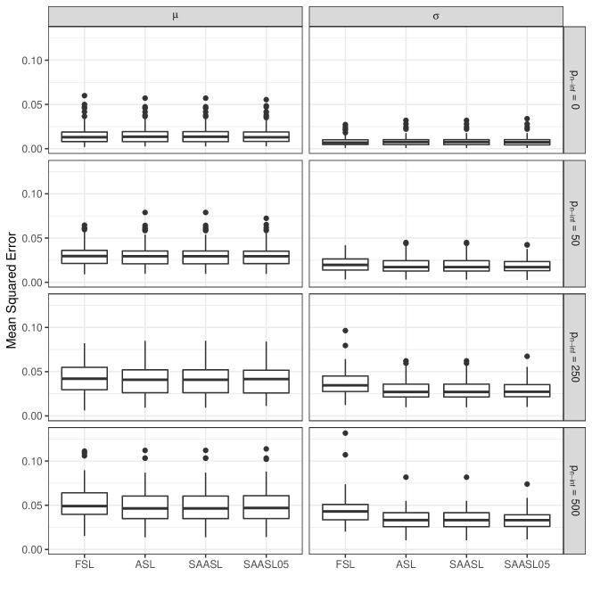
Figure 4.1: Comparison between mean squared error for FSL and the three ASL methods. The left column comprises the MSE for $\eta_{\boldsymbol{\mu}}$, the right column for $\eta_{\boldsymbol{\sigma}}$. The different numbers of non-informative variables are represented row-wise.

Figure 4.1 shows the comparison of the mean squared error (MSE) among non-cyclical boosted algorithms for $\boldsymbol{\mu}$ and $\boldsymbol{\sigma}$, where the MSEs are defined on the predictor level as $\text{MSE}_{\boldsymbol{\mu}}=\frac{1}{n}\sum_{i=1}^{n}(\mu_{i}-\eta_{\boldsymbol{\mu}}(\boldsymbol{x}_{i\cdot}))^{2}$ and $\text{MSE}_{\boldsymbol{\sigma}}=\frac{1}{n}\sum_{i=1}^{n}(\log(\sigma_{i})-\eta_{\boldsymbol{\sigma}}(\boldsymbol{x}_{i\cdot}))^{2}$, respectively. In general, all methods have a similar MSE, with the MSE of FSL increasing more strongly with the number of non-informative variables $p_{\text{n-inf}}$ and ASL methods hence slightly outperform FSL in the variance predictor for a high number of non-informative variables. ASL and SAASL show identical results, as they should if the line search is correctly conducted, with results returned by SAASL05 very similar.

Computing the negative log-likelihood in sample of the model fits reveals a slight advantage for FSL (see Appendix Figure B.3). However, this can be linked to the fact that FSL selects more false positive variables on average than the adaptive approaches and thus shows a relatively stronger tendency to overfit the training data (Figure 4.2).

For $\boldsymbol{\sigma}$, even if $p_{\text{n-info}}$ is small, the false positive rates of the adaptive approaches are notably smaller than those of FSL. As discussed above, $\nu_{j^{*},\boldsymbol{\sigma}}^{[m]}\approx 0.05$ for large $m$ in the adaptive approach is smaller than $\nu_{\boldsymbol{\sigma}}=0.1$ for FSL. An update with a smaller, conservative step-length can apparently help to avoid overfitting and the adaptive step-length here seems to strike the balance between learning speed and the number of false positives. While it would also be possible to lower the step-length for FSL to reduce the number of non-informative variables included in the final model, this would increase the number of boosting iterations and the computing time, and it would not address the imbalance between updates for $\boldsymbol{\mu}$ and $\boldsymbol{\sigma}$. The optimal choice of the step-length is also difficult without further tuning or an automatic selection as in ASL.

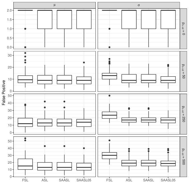
Figure 4.2: Comparison between false positives for FSL and the three ASL methods. The left column comprises the false positives for $\boldsymbol{\mu}$, the right column for $\boldsymbol{\sigma}$. The different numbers of non-informative variables settings are represented row-wise.

In Figure 4.3 we show an example of the comparison between the optimal step-lengths in this case. As can be seen, the step-lengths for $\boldsymbol{\sigma}$ (depicted in grey) converge to $0.5$ as shown in section 3.2.2. The second fact that becomes obvious when looking at the figure is that the optimal step-lengths for both predictors do not differ a lot. Even though differences can be observed in early iterations in particular, the step-lengths still have the same order of magnitude. This is not only the case for this example but overall in this simulation setup. Having this in mind, the similar results for both approaches (FSL and ASL) are not very surprising anymore: there is hardly any difference in the approaches, since the updates do not need different step-lengths to be balanced. In the next subsection we will examine a case in which the data calls for different step-lengths, and see how both methods perform under those changed circumstances.

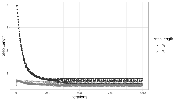
Figure 4.3: Comparison of the optimal step-lengths $\nu_{j^{*},\boldsymbol{\mu}}^{*[m]}$ and $\nu_{j^{*},\boldsymbol{\sigma}}^{*[m]}$ in SAASL from one of the $100$ simulation runs. The step-lengths for $\mu$ are in black dots, the step-lengths for $\sigma$ in grey cross. Different horizontal layers of dots/crosses correspond to different covariates.

4.2 Large Variance with resulting Imbalance between Location and Scale

As discussed above, the Gaussian location and scale model in section 4.1 did not lead to a large difference between FSL and ASL, as the optimal step-lengths for $\boldsymbol{\mu}$ and $\boldsymbol{\sigma}$ were roughly similar and the imbalance between the updates for the two predictors in FSL was thus not large. In this section, we investigate a setting with a large variance, which leads to a stronger imbalance between the two parts of the model.

In the following, we use SAASL as a representative of the adaptive approaches in our presentation, as it yields identical results to ASL, but avoids the numerical search for the optimal $\nu_{\boldsymbol{\mu}}$ by using the analytical result (5). Since estimated effects generally deviated more strongly from the theoretical values than before due to the large variance (details will be discussed later), we additionally compared the results to those obtained using GAMLSS with penalized maximum likelihood estimation as implemented in the R-package gamlss [Rigby and Stasinopoulos (2005)].

Consider the data generating mechanism $y_{i}\sim N(\mu_{i},\sigma_{i}),i\in\{1,\cdots,500\}$ with $B=100$ simulation runs. The predictors are determined by

$$\eta_{\boldsymbol{\mu}}(\boldsymbol{x}_{i\cdot}) =\mu_{i}=1+x_{i1}+2x_{i2}-x_{i3}$$

$$\eta_{\boldsymbol{\sigma}}(\boldsymbol{x}_{i\cdot}) =\log(\sigma_{i})=5+0.1x_{i1}-0.2x_{i2}+0.1x_{i3},$$

where $\boldsymbol{x}_{\cdot j}\sim\text{Uni}(-1,1),j\in\{1,2,3,4,5\}$, $\boldsymbol{x}_{\cdot 4}$ and $\boldsymbol{x}_{\cdot 5}$ are noise variables. Note that this choice of $\eta_{\boldsymbol{\sigma}}$ leads to an extremely large standard deviation in the order of 150 due to the large intercept 5. The stopping iteration is obtained by 10-fold CV, and the maximum number of iterations is 3000 and 2,000,000 for SAASL and FSL respectively.

As can be seen in Figure 4.4, both fixed and adaptive step-lengths yield reasonable estimates regarding $\eta_{\boldsymbol{\sigma}}$, but FSL results in many false negative estimates equal to zero for $\eta_{\boldsymbol{\mu}}$ in the majority of the simulation runs. This is of course connected to the relative importance of the variance component in this setting, which should in itself already lead to a preference for updating $\eta_{\boldsymbol{\sigma}}$ rather than $\eta_{\boldsymbol{\mu}}$ in early boosting iterations due to the fact that the negative gradient for $\boldsymbol{\mu}$ (i.e. $u_{\boldsymbol{\mu},i}=\sum_{i=1}^{n}(y_{i}-\mu_{i})/\sigma_{i}^{2}\text{ with large }\sigma_{i}$) is actually scaled by the variance (recall the large intercept 5, log-link and the resulting exponential transformation) and hence very small. As a consequence, the impact on the global loss of base-learners fit to the gradient is also small compared to those suggested for updates regarding $\sigma$ in step 11 of Algorithm 2.3. Then, using the same step-length for both parameters makes it clearly harder to identify informative effects on $\mu$ as they are trivialized in comparisons.

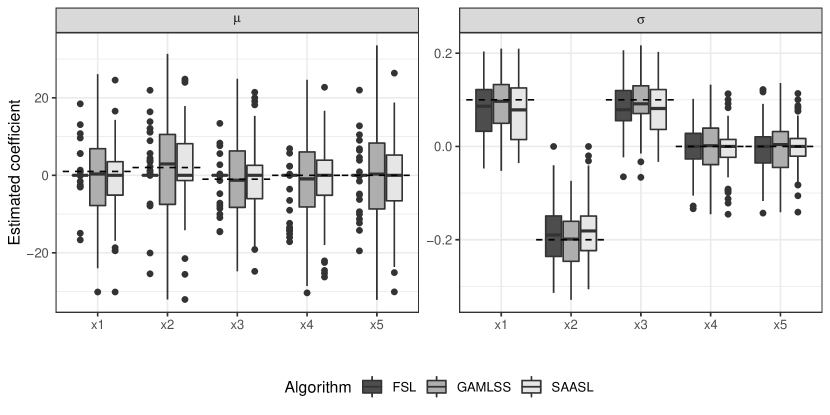
Figure 4.4: Distribution of coefficient estimates from $B=100$ simulation runs. The true coefficients are marked by the dashed horizontal lines.

The adaptive step-lengths implemented in SAASL compensates for this disadvantage. Compared to the simulation results in the previous subsection the estimates regarding $\eta_{\boldsymbol{\mu}}$ are less precise with large variability around the true values. This is not a problem of SAASL but again the consequence of the large variance, obscuring the effects on the mean, and also encountered using the penalized maximum likelihood approach implemented in the gamlss-package (called GAMLSS in Figure 4.4). The variability in the estimates is actually somewhat smaller than for GAMLSS due to the regularization inherent in the boosting approach. This is also illustrated in Figure 4.5 in the pairwise comparison of the estimated coefficients for both methods, where SAASL leads to similar but slightly closer to zero estimates compared to the penalized maximum likelihood based method GAMLSS.

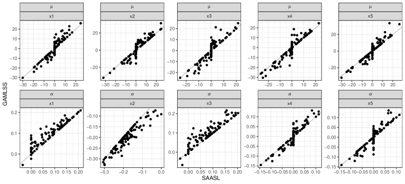
Figure 4.5: Pairwise comparison of the estimated coefficients between GAMLSS and SAASL.

Interestingly, Figure 4.4 also reveals that the inability to identify the informative variables results in the lowest MSE for all three individual coefficients for $\boldsymbol{\mu}$ when using FSL (for more numerical details, see Appendix C). As can be seen from Table 4.1, however, the combined additive predictor performs worse in terms of overall MSE than both GAMLSS and SAASL, with the latter performing best.

Table 4.1: Summary of the in-sample MSE for each estimation methods, i.e. $\frac{1}{n}\sum_{i=1}^{n}\left(y_{i}-\hat{y}_{i}\right)^{2}$.

	Min.	1st Qu.	Median	Mean	3rd Qu.	Max.
FSL	19848	21796	22547	22688	23579	27026
GAMLSS	19707	21687	22414	22586	23515	26883
SAASL	19679	21663	22372	22554	23443	26883

To further highlight the differences in the selection behavior between FSL and SAASL, Figure 4.6 illustrates the proportion of boosting iterations used to update $\boldsymbol{\mu}$ over the course of the model fits, i.e. $p_{m_{\boldsymbol{\mu}}}=m_{\boldsymbol{\mu}}/(m_{\boldsymbol{\mu}}+m_{\boldsymbol{\sigma}})$, where $m_{\boldsymbol{\mu}}+m_{\boldsymbol{\sigma}}=m_{\text{stop}}$. The bimodal distribution for FSL observed in the histogram in panel (6(a)) demonstrates another problem of the fixed step-lengths in this setting. Considering the many estimates equal or close to zero observed in Figure 4.4, the mode close to $p_{m_{\boldsymbol{\mu}}}=0$ is expected, as it describes the proportion of simulation runs where $\mu$ has not been updated at all. However, as soon as at least one base-learner for $\boldsymbol{\mu}$ is recognized as an effective model parameter, the small step-length fixed at 0.1 requires a huge number of updates for the base-learner to actually make an impact on the global loss (hence the large number of maximum iterations allowed for FSL). This results in the second mode also around $p_{m_{\boldsymbol{\mu}}}=1$, as the algorithm is mainly occupied with $\mu$ in the corresponding runs.

This is illustrated by the scatter plot in Figure 4.6(6(b)), where $p_{m_{\boldsymbol{\mu}}}$ is plotted against the stopping iteration $m_{\text{stop}}$. Note that the y-axis is displayed with a logarithmic scale and each tick on the y-axis represents a tenfold increase over the previous one. The few points (FSL), whose $m_{\text{stop}}$ lie between $10^{2}$ and $10^{3}$, show a better balance between the updates of $\boldsymbol{\mu}$ and $\boldsymbol{\sigma}$ than other points, i.e., the middle region of $p_{m_{\boldsymbol{\mu}}}$. But we also observe a bimodal distribution for FSL, i.e., lots of points are equal or close to $p_{m_{\mu}}=0$ and 1, with very low and extremely large values for $m_{\text{stop}}$ resulting, respectively.

For SAASL, the distribution of $p_{m_{\boldsymbol{\mu}}}$ in Figure 4.6(6(a)) is unimodal. The mode smaller than 0.5 indicates SAASL updates $\boldsymbol{\sigma}$ a little more frequently than $\boldsymbol{\mu}$. Unlike the cyclical approach that enforces an equal number of updates for all distribution parameters, the balance formed by SAASL is more natural. This balance enables the alternate updates between two predictors even though they lie on different scales. Therefore, the information in $\boldsymbol{\mu}$ can be fairly discovered in time and it reduces the risk of overlooking the informative base-learners with respect to $\boldsymbol{\mu}$. The number of simulations runs, in which $\boldsymbol{\mu}$ is not updated at all ($p_{m_{\boldsymbol{\mu}}}=0$), reduces from 39 in FSL to only 5 in SAASL. Moreover, none of the 100 simulations require a substantial amount of updates for $\boldsymbol{\mu}$ to get well estimated coefficients (cf. also Figure 4.4).

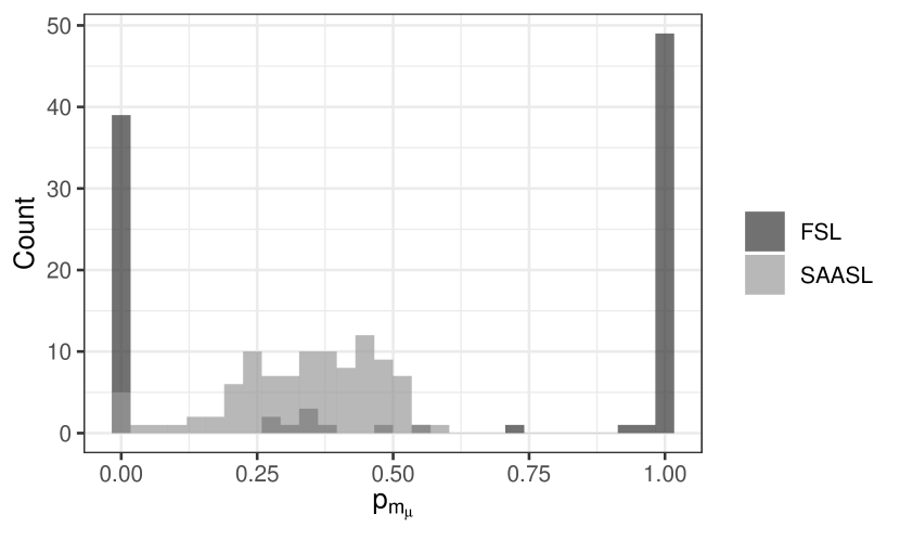
(a) Histogram

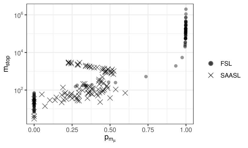
(b) Scatter plot

Figure 4.6: Distribution of $p_{m_{\boldsymbol{\mu}}}$ in $B=100$ simulation runs. (6(a)) Histogram of $p_{m_{\boldsymbol{\mu}}}$. The histogram of the two approaches are overlayed using transparency. (6(b)) Scatter plot of $m_{\text{stop}}$ against $p_{m_{\boldsymbol{\mu}}}$. Points and crosses are displayed with transparency. The $y$-axis is displayed on a logarithmic scale with base 10. Each tick represents a tenfold increase over the previous one.

Table 4.2 displays the information about false positives and false negatives of the two approaches in all 100 simulations with respect to $\boldsymbol{\mu}$ and $\boldsymbol{\sigma}$. For example, the second and fourth number 77 and 21 in the first line indicate that the informative variable $\boldsymbol{x}_{\cdot 2}$ is not included in the final model in 77 out of 100 simulation runs (i.e. false negative), while there are 21 simulations whose final model contains the non-informative variable $\boldsymbol{x}_{\cdot 4}$ (i.e. false positive). Similar as Figure 4.2 in section 4.1, the conservative small step-length for $\boldsymbol{\mu}$ in FSL increases the number of boosting iterations, but reduces the risk of overfitting. Less simulations containing the noise variables for $\boldsymbol{\mu}$ in FSL than in SAASL confirms this behavior. According to equation (11) the ASLs $\nu_{j^{*},\boldsymbol{\sigma}}$ are a sequence of values around 0.05, and (except for the values at early boosting iterations) most of them smaller than 0.1. There are correspondingly slightly more simulations in FSL overfitting the $\boldsymbol{\sigma}$-submodel than in SAASL.

Table 4.2: The number of simulations with false positives and false negatives for each variable under different modelling methods with respect to the two model parameters. The false negatives part shows the number of simulations in which the informative variables are excluded from the final model, and the false positives part shows how many simulations include the non-informative variables in their final model. Values are taken at the stopping iteration determined by 10-fold CV.

		False Negatives			False Positives
		$\boldsymbol{x}_{\cdot 1}$	$\boldsymbol{x}_{\cdot 2}$	$\boldsymbol{x}_{\cdot 3}$	$\boldsymbol{x}_{\cdot 4}$	$\boldsymbol{x}_{\cdot 5}$
$\mu$	FSL	83	77	81	21	20
	SAASL	28	24	28	72	73
$\sigma$	FSL	9	1	6	83	82
	SAASL	18	1	9	70	67

Although non-informative variables of $\boldsymbol{\mu}$ are excluded from the FSL model, the informative ones are excluded as well. Actually $\boldsymbol{\mu}$ was not updated in many simulations at all (cf. Figure 4.6(6(a))). The false negatives part of Table 4.2 for $\boldsymbol{\mu}$ confirms this. The informative variables $\boldsymbol{x}_{\cdot 1}$ to $\boldsymbol{x}_{\cdot 3}$ are excluded from the final model in the majority of simulations with FSL but not with SAASL. For $\boldsymbol{\sigma}$, the smaller step-length $\nu_{j^{*},\boldsymbol{\sigma}}$ in SAASL selects variables more conservatively and as a consequence slightly more simulations underfit the $\boldsymbol{\sigma}$-submodel in SAASL than in FSL, but the difference is far less pronounced.

5 Applications

We apply the proposed algorithms to two datasets. The malnutrition dataset demonstrates the shortcomings of FSL and the pitfalls of using numerical determination of ASL with a fixed search interval, and with the riboflavin dataset we illustrate the variable selection properties of each algorithm.

5.1 Malnutrition of children in India

The first data called india from the R package gamboostLSS [Hofner et al. (2018); Fahrmeir and Kneib (2011)] are sampled from the Standard Demographic and Health Survey between 1998 and 1999 on malnutrition of children in India [Fahrmeir and Kneib (2011)]. The sample contains 4000 observations and four variables (BMI of the child (cBMI), age of the child in months (cAge), BMI of the mother (mBMI) and age of the mother in years (mAge)). The outcome of interest in this case is a numeric z-score for malnutrition ranging from -6 to 6, where the negative values represent malnourished children. To highlight the problems of using a fixed step-length, we work with the original variable stunting (corresponding to 100 * z-score). The identity and logarithm functions are used as the link functions for $\boldsymbol{\mu}$ and $\boldsymbol{\sigma}$ respectively.

Because this is not a high-dimensional data example, we use the GAMLSS with penalized maximum-likelihood estimation as a gold standard to examine the effectiveness of the adaptive approaches.

Table 5.1 lists the estimated coefficients of each variable on the predictors $\eta_{\boldsymbol{\mu}}$ and $\eta_{\boldsymbol{\sigma}}$ at the stopping iteration tuned by 10-folds CV, where the maximum number of iterations is set to 2000. The estimated intercept in $\eta_{\boldsymbol{\sigma}}$ indicates a large variance of the response, with the setting thus being similar to the second simulation above. It is therefore not surprising that FSL selects only one variable (cAge) for $\eta_{\boldsymbol{\mu}}$, i.e. a large number of updates for the base-learner are required but the given maximal boosting iteration is not large enough. In practice we can certainly increase the maximum number of iterations as well as enlarge the commonly applied step-length 0.1 in order to estimate the coefficients well. But their choices are very subjective and probably result in tedious manual fine-tuning based on trial and error.

The ASL method with the default predefined search interval $[0,10]$ encounters a similar problem as FSL. Apart from the only selected and underfitted variable cAge for $\boldsymbol{\mu}$, the two variables (cBMI and cAge) for the $\boldsymbol{\sigma}$-submodel are also underfitted compared with the results from the gold standard GAMLSS. The reason for this phenomenon lies in the relationship between the variance and step-length discussed in equation (5). The log-link or exponential transformation for $\eta_{\boldsymbol{\sigma}}$ in this example data requires a sequence of huge step-lengths, but the default search interval does not fulfill this requirement.

An estimation of ASL by increasing its search interval to $[0,50000]$, denoted as ASL5 in Table 5.1, results in coefficients comparable to those of GAMLSS. But choosing a suitable search interval becomes an unavoidable side task for ASL when analyzing this kind of dataset.

The results of the two semi-analytical approaches hardly differ from the maximum likelihood based GAMLSS. Unlike the numerical determination with a fixed search interval in ASL, the analytical approaches replace this procedure with a direct and precise solution that gets rid of the potential manual intervention (e.g. increasing the search interval). Contrary to the direct influence of the variance on $\nu_{j^{*},\boldsymbol{\mu}}^{*[m]}$ in equation (5), the optimal step-length $\nu_{j^{*},\boldsymbol{\sigma}}^{*[m]}$ is dominated by the chosen base-learner, but as the number of learning iterations increases, such effects gradually disappear, and $\nu_{j^{*},\boldsymbol{\sigma}}^{*[m]}$ finally converges to 0.5. Thus, our default search interval $[0,1]$ is sufficient for $\nu_{j^{*},\boldsymbol{\sigma}}^{*[m]}$, and increasing the range of search interval as for $\nu_{j^{*},\boldsymbol{\mu}}^{*[m]}$ in ASL is almost never necessary.

Theoretically, the ASL with a sufficiently large search interval (ASL5 in this example) and SAASL should result in the same values as discussed in the previous theoretical section. Due to the calculation accuracy of computers and the numerical optimization steps, their outputs are very similar but can differ slightly for the malnutrition data.

Table 5.1: Comparison of the estimated coefficients.

		FSL	ASL	ASL5	SAASL	SAASL05	GAMLSS
(Intercept)	$\eta_{\boldsymbol{\mu}}$	-174.77179	-169.20269	-91.16032	-91.16011	-91.16041	-91.15953
	$\eta_{\boldsymbol{\sigma}}$	4.88080	4.87412	4.91206	4.91207	4.91206	4.91205
cBMI	$\eta_{\boldsymbol{\mu}}$	0.00000	0.00000	-13.92524	-13.92509	-13.92526	-13.92552
	$\eta_{\boldsymbol{\sigma}}$	-0.00319	-0.00268	-0.01527	-0.01526	-0.01527	-0.01526
cAge	$\eta_{\boldsymbol{\mu}}$	-0.03845	-0.37092	-5.84669	-5.84665	-5.84670	-5.84663
	$\eta_{\boldsymbol{\sigma}}$	-0.00103	-0.00074	0.00284	0.00284	0.00284	0.00284
mBMI	$\eta_{\boldsymbol{\mu}}$	0.00000	0.00000	11.70780	11.70770	11.70782	11.70787
	$\eta_{\boldsymbol{\sigma}}$	0.00897	0.00875	0.00864	0.00864	0.00864	0.00864
mAge	$\eta_{\boldsymbol{\mu}}$	0.00000	0.00000	0.02570	0.02564	0.02571	0.02575
	$\eta_{\boldsymbol{\sigma}}$	0.00537	0.00513	0.00530	0.00530	0.00530	0.00530

Figure 5.1 presents the optimal step-lengths $\nu_{j^{*},\boldsymbol{\mu}}^{*[m]}$ and $\nu_{j^{*},\boldsymbol{\sigma}}^{*[m]}$ using SAASL for each variable up to 769 boosting iterations specified by 10-folds CV for one simulation run. Apparently, the optimal step-lengths for $\boldsymbol{\mu}$ over the entire learning process are over 20000, which is far larger than the fixed step-length 0.1 and the upper boundary 10 of the predefined search interval in ASL. Without knowing this information, it is not trivial to determine the search interval for $\nu_{j^{*},\boldsymbol{\mu}}^{*[m]}$. And we thus (after acquiring this graphic) re-estimated the example data with ASL5.

Additionally, Figure 5.1(1(b)) illustrates the optimal step-length for $\boldsymbol{\sigma}$. After several boosting iterations the optimal values of each covariate converge to their own stable regions (ranging from about 0.38 to 0.56). As discussed above, the optimal step-lengths for $\boldsymbol{\sigma}$ should be some values around 0.5, and this graphic confirms this statement.

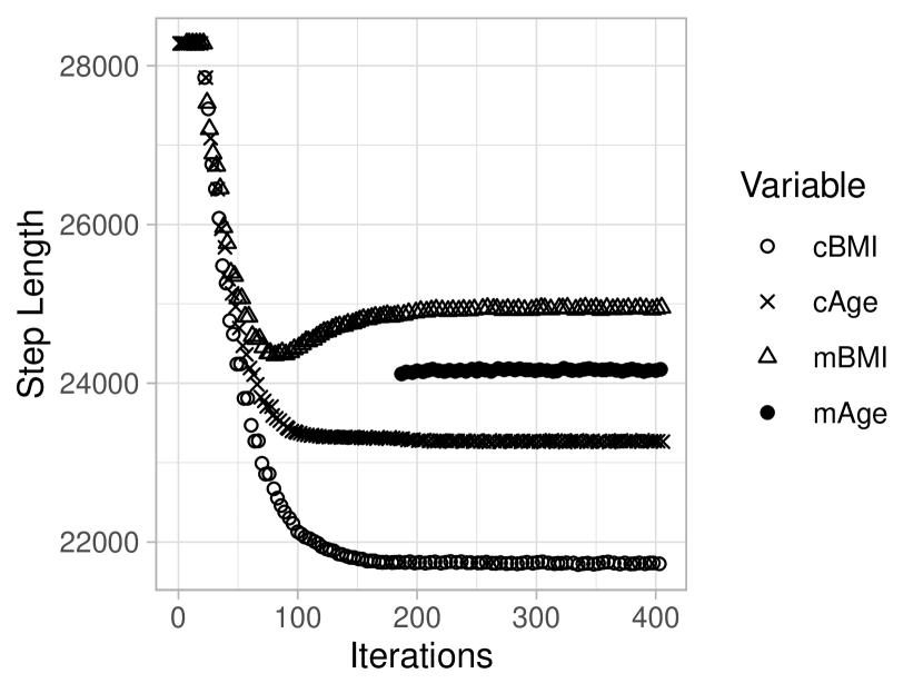
(a) $\nu_{j^{*},\boldsymbol{\mu}}^{*[m]}$

(b) $\nu_{j^{*},\boldsymbol{\sigma}}^{*[m]}$

Figure 5.1: The optimal step-length of each model parameters against the boosting iterations. Up to the stopping iterations specified by 10-folds CV (here $m_{\text{stop}}=769$), 406 iterations are used to update $\boldsymbol{\mu}$ and 363 iterations are used to update $\boldsymbol{\sigma}$.

As this example is not high-dimensional and does not necessarily require variable selection, we can use GAMLSS with penalized maximum likelihood estimation for comparison. The fact that its results are very similar to those of the semi-analytical approaches indicates that results from SAASL and SAASL05 are reliable. The only alternative to achieve balance between predictors would be using a cyclical algorithm (with the downsides discussed in the introduction). Rescaling the response variable or standardizing the negative partial derivatives could reduce the scaling problem to some extend, but would not eliminate the need to increase the step-length or reduce the imbalance between predictors.

5.2 Riboflavin dataset

This data set describes the riboflavin (also known as vitamin $B_{2}$) production by Bacillus subtilis, containing 71 observations and 4088 predictors (gene expressions) [Bühlmann et al. (2014); Dezeure et al. (2015)]. The log-transformed riboflavin production rate, which is close to a Gaussian distribution, is regarded as the response. This data set is chosen to demonstrate the capability of the boosting algorithm to deal with situations in which the number of covariates exceeds the number of observations. Please note that a comparison to the original GAMLSS algorithm is not possible in this case, since the algorithm is not able to deal with more model parameters than available observations. In order to compare the out-of-sample MSE of each algorithm, we select 10 observations randomly as the validation set.

Table 5.2 summarize the selected informative variables for $\boldsymbol{\mu}$ and $\boldsymbol{\sigma}$ separately at the stopping iteration tuned by 5-fold CV, the corresponding coefficients are listed in Appendix D. The results in both tables demonstrate the intersection of the selected variables, for example FSL selects 13 informative variables in total, and 9 of them are also chosen by ASL and SAASL, and there are 11 variables common with SAASL05. In general, for both $\boldsymbol{\mu}$ and $\boldsymbol{\sigma}$, more variables are included in the adaptive approaches and the difference in the selected variables mainly lies between the adaptive and fixed approach. Because the optimal step-length $\nu_{j^{*},\boldsymbol{\mu}}^{*[m]}$ lies in the predefined search interval $[0,10]$ (and is actually smaller than 1, i.e. the adaptive step-length $\nu_{j^{*},\boldsymbol{\mu}}^{[m]}<0.1$), and $\nu_{j^{*},\boldsymbol{\sigma}}^{*[m]}$ lies also in a narrower predefined search interval $[0,1]$, ASL and SAASL have the same results. Moreover, as the adaptive step-length is smaller than the fixed step-length 0.1, the adaptive approaches make conservative (small) updates, leading to more boosting iterations. Several of the gene expressions for $\boldsymbol{\mu}$ and $\boldsymbol{\sigma}$ are selected by all algorithms and are thus consistently included in the set of informative covariates. Actually almost all gene expressions chosen by FSL are also recognized as informative variables by all other methods.

Table 5.2: Number of chosen variables for $\eta_{\boldsymbol{\mu}}$ and $\eta_{\boldsymbol{\sigma}}$. The diagonal depicts the number per method, the off-diagonal elements overlapping variables.

	$\eta_{\boldsymbol{\mu}}$				$\eta_{\boldsymbol{\sigma}}$
	FSL	ASL	SAASL	SAASL05	FSL	ASL	SAASL	SAASL05
FSL	13	9	9	11	16	9	9	12
ASL	9	20	20	18	9	17	17	15
SAASL	9	20	20	18	9	17	17	15
SAASL05	11	18	18	24	12	15	15	24

To compare the performance of each algorithm, Table 5.3 lists the out-of-sample MSE. In contrast to the fixed approach, the three adaptive approaches perform in general well, where the performance of SAASL05 is slightly worse than the other two. In addition, table 5.3 demonstrates also the result of Lasso estimator from the R package glmnet [Friedman et al. (2010)] suggested by Bühlmann et al. (2014). The mean squared prediction error of glmnet is the smallest among the five approaches, but the difference with the adaptive approaches is relatively small.

Table 5.3: Out-of-sample MSE.

	FSL	ASL	SAASL	SAASL05	glmnet
MSE	2.611	1.111	1.111	1.193	0.946

As glmnet cannot model the scale parameter $\boldsymbol{\sigma}$, only the estimated coefficients of the $\boldsymbol{\mu}$-submodel are provided in Appendix D. Out of the 21 genes selected by glmnet, 7 and 9 of them are common with the ASL/SAASL and SAASL05, respectively. The signs (positive/negative) of the estimated coefficients of these common covariates from glmnet match the adaptive approaches. This comparison indicates that the boosted GAMLSS with adaptive step-length is an applicable and competitive approach for high-dimensional data analysis.

6 Conclusions and Outlook

The step-length is often not treated as an important tuning parameter in many boosting algorithms, as long as it is set to a small value. However, if complex models like GAMLSS with several predictors for the different distribution parameters are estimated, the different scales of the distribution parameters can lead to imbalanced updates and resulting bad performances if one common small fixed step-length is used, as we show in this paper.

The main contribution of this article is the proposal to use separate adaptive step-lengths for each distribution parameter in a non-cyclical boosting algorithm for GAMLSS, which are optimized in each iteration. In addition to the resulting balance in updates between different distribution parameters, a balance between over- and underfitting is obtained by taking only a proportion (shrinkage parameter) such as 10% of the determined optimal step-length as the adaptive step-length. The optimal step-length can be found by optimization procedures such as a line search. We illustrated with an example the importance of updating the search interval for the search if necessary to find the optimal solution.

For the important special case of the Gaussian distribution, we derived an analytical solution for the adaptive step-length for the mean parameter $\boldsymbol{\mu}$, which avoids numerical optimization and specification of a search interval. For the scale parameter $\boldsymbol{\sigma}$, we obtained an approximate solution of 0.5 (or 0.05 with 10% proportion), which gives a better motivated default value than 0.1 relative to the step-length for $\boldsymbol{\mu}$, and discussed a combination with a one-dimensional line search in the semi-analytical approach.

In simulations and empirical applications, we showed favorable behavior compared to using a fixed step-length FSL. We showed highly competitive results of our adaptive approaches compared to a standard GAMLSS with respect to estimation accuracy for the low-dimensional case, while the adaptive boosting approach has the advantages of shrinkage and variable selection, which makes it also applicable to the high-dimensional case of more covariates than observations. Overall, the semi-analytical method for adaptive step-length selection performed best among the considered methods.

In this paper we focused on the special case of the Gaussian distribution to derive analytical or semi-analytical solutions for the optimal step-length. In other cases, a line search has to be conducted for all distribution parameters. In the future, it is worth investigating to derive analytical adaptive step-lengths for other distributions as well, because analytical or approximate adaptive step-lengths increase the numerical efficiency and also reveal the relationships between the optimal step-lengths for different parameters and model parameters (as well as properties of commonly used but probably less than ideal step-length settings).

Further work should also be the implementation of further (e.g. non-linear, spatial etc.) effects [Hothorn et al. (2011)] into the model, and test the influence of the adaptive step-length on such effects. Moreover, we discovered correlations between the optimal step-length $\nu_{j^{*},\boldsymbol{\mu}}^{*[m]}$ of a variable and the coefficient of this variable in the $\boldsymbol{\sigma}$-submodel through our application of the algorithm. Future work should also investigate the relationship among the optimal step-lengths of different parameters and the relationship of these step-lengths to the model coefficients.

A basic R package ASL based on this article is available online at https://github.com/FAUBZhang/ASL. This package contains the source code of Algorithm 3.3 and the function of the corresponding cross-validation. Some simple examples can also be found in this package. This package is originated from the R package gamboostLSS, we hope to implement the functions of ASL into the latter in the future.

Acknowledgements

The work on this article was supported by the Freigeist-Fellowships of Volkswagen Stiftung, project “Bayesian Boosting - A new approach to data science, unifying two statistical philosophies”. Boyao Zhang performed the present work in partial fulfilment of the requirements for obtaining the degree “Dr. rer. biol. hum.” at the Friedrich-Alexander-Universität Erlangen-Nürnberg (FAU).

Appendix A Derive the analytical ASL for the Gaussian distribution

Take the negative log-likelihood as the loss function, the loss for Gaussian distribution can be displayed as

$$\rho\left(\boldsymbol{y},\{\eta_{\boldsymbol{\mu}},\eta_{\boldsymbol{\sigma}}\}\right)= -\log\left[\frac{1}{\left(\sqrt{2\pi}\right)^{n}}\det\left(\operatorname{diag}\left(\exp\left(-\eta_{\boldsymbol{\sigma}}(\boldsymbol{X})\right)\right)\right)\cdot\right.$$

$$\left.\cdot\exp\left(-\frac{1}{2}(\boldsymbol{y}-\eta_{\boldsymbol{\mu}}\left(\boldsymbol{X})\right)^{T}\operatorname{diag}\left(\exp\left(-2\eta_{\boldsymbol{\sigma}}(\boldsymbol{X})\right)\right)(\boldsymbol{y}-\eta_{\boldsymbol{\mu}}(\boldsymbol{X}))\right)\right]$$

$$= \frac{n}{2}\log(2\pi)+\boldsymbol{1}_{n}^{T}\eta_{\boldsymbol{\sigma}}(\boldsymbol{X})+\frac{1}{2}\left(\boldsymbol{y}-\eta_{\boldsymbol{\mu}}(\boldsymbol{X})\right)^{T}\operatorname{diag}\left(\exp\left(-2\eta_{\boldsymbol{\sigma}}(\boldsymbol{X})\right)\right)\left(\boldsymbol{y}-\eta_{\boldsymbol{\mu}}(\boldsymbol{X})\right).$$

The negative partial derivatives for both distribution parameters in iteration $m$ are then

$$\boldsymbol{u}_{\boldsymbol{\mu}}^{[m]} =-\frac{\partial\rho\left(\boldsymbol{y},\{\hat{\eta}_{\boldsymbol{\mu}}^{[m-1]},\hat{\eta}_{\boldsymbol{\sigma}}^{[m-1]}\}\right)}{\partial\hat{\eta}_{\boldsymbol{\mu}}}$$ (12)

$$=\operatorname{diag}\left(\exp\left(-2\hat{\eta}_{\boldsymbol{\sigma}}^{[m-1]}(\boldsymbol{X})\right)\right)\left(\boldsymbol{y}-\hat{\eta}_{\boldsymbol{\mu}}^{[m-1]}(\boldsymbol{X})\right),$$ (13)

$$\boldsymbol{u}_{\boldsymbol{\sigma}}^{[m]} =-\frac{\partial\rho\left(\boldsymbol{y},\{\hat{\eta}_{\boldsymbol{\mu}}^{[m-1]},\hat{\eta}_{\boldsymbol{\sigma}}^{[m-1]}\}\right)}{\partial\hat{\eta}_{\boldsymbol{\sigma}}}$$ (14)

$$=-\boldsymbol{1}_{n}+\operatorname{diag}\left(\left(\boldsymbol{y}-\hat{\eta}_{\boldsymbol{\mu}}^{[m-1]}(\boldsymbol{X})\right)^{T}\right)\operatorname{diag}\left(\exp\left(-2\hat{\eta}_{\boldsymbol{\sigma}}^{[m-1]}(\boldsymbol{X})\right)\right)\left(\boldsymbol{y}-\hat{\eta}_{\boldsymbol{\mu}}^{[m-1]}(\boldsymbol{X})\right).$$ (15)

Both $\boldsymbol{u}_{\boldsymbol{\theta}}^{[m]},\boldsymbol{\theta}\in\{\boldsymbol{\mu},\boldsymbol{\sigma}\}$ can be regressed on the simple linear base-learner $h_{j^{*},\boldsymbol{\theta}}^{[m]}(\boldsymbol{x}_{\cdot j^{*}})$, where $j^{*}$ denotes the best-fitting variable.

$$\boldsymbol{u}_{\boldsymbol{\mu}}^{[m]} =\hat{h}_{j^{*},\boldsymbol{\mu}}^{[m]}(\boldsymbol{x}_{\cdot j^{*}})+\hat{\boldsymbol{\epsilon}}_{\boldsymbol{\mu}}^{[m]}$$ (16)

$$\boldsymbol{u}_{\boldsymbol{\sigma}}^{[m]} =\hat{h}_{j^{*},\boldsymbol{\sigma}}^{[m]}(\boldsymbol{x}_{\cdot j^{*}})+\hat{\boldsymbol{\epsilon}}_{\boldsymbol{\sigma}}^{[m]},$$ (17)

where $\hat{\boldsymbol{\epsilon}}_{\boldsymbol{\mu}}^{[m]}$ and $\hat{\boldsymbol{\epsilon}}_{\boldsymbol{\sigma}}^{[m]}$ denote the residuals in simple linear regression models.

A.1 Optimal step-length for $\boldsymbol{\mu}$

The analytical optimal step-length for $\boldsymbol{\mu}$ in iteration $m$ is obtained by minimizing the empirical risk,

$$\nu^{*[m]}_{j^{*},\boldsymbol{\mu}} =\operatorname*{arg\,min}_{\nu}\sum_{i=1}^{n}\rho\left(y_{i},\{\hat{\eta}_{\boldsymbol{\mu}}^{[m]}(\boldsymbol{x}_{i\cdot}),\hat{\eta}_{\boldsymbol{\sigma}}^{[m-1]}(\boldsymbol{x}_{i\cdot})\}\right)$$

$$=\operatorname*{arg\,min}_{\nu}\sum_{i=1}^{n}\rho\left(y_{i},\{\hat{\eta}_{\boldsymbol{\mu}}^{[m-1]}(\boldsymbol{x}_{i\cdot})+\nu\hat{h}_{j^{*},\boldsymbol{\mu}}^{[m]}(x_{ij^{*}}),\hat{\eta}_{\boldsymbol{\sigma}}^{[m-1]}(\boldsymbol{x}_{i\cdot})\}\right)$$

$$=\operatorname*{arg\,min}_{\nu}\sum_{i=1}^{n}-\log\left[\frac{1}{\sqrt{2\pi}\exp(\hat{\eta}_{\boldsymbol{\sigma}}^{[m-1]}(\boldsymbol{x}_{i\cdot}))}\exp\left(-\frac{\left(y_{i}-\hat{\eta}_{\boldsymbol{\mu}}^{[m-1]}(\boldsymbol{x}_{i\cdot})-\nu\hat{h}_{j^{*},\boldsymbol{\mu}}^{[m]}(x_{ij^{*}})\right)^{2}}{2\exp(2\hat{\eta}_{\boldsymbol{\sigma}}^{[m-1]}(\boldsymbol{x}_{i\cdot}))}\right)\right]$$

$$=\operatorname*{arg\,min}_{\nu}\sum_{i=1}^{n}\left[\frac{1}{2}\log(2\pi)+\log(\hat{\sigma}_{i}^{[m-1]})+\frac{\left(y_{i}-\hat{\eta}_{\boldsymbol{\mu}}^{[m-1]}(\boldsymbol{x}_{i\cdot})-\nu\hat{h}_{j^{*},\boldsymbol{\mu}}^{[m]}(x_{ij^{*}})\right)^{2}}{2\sigma_{i}^{2[m-1]}}\right]$$

$$=\operatorname*{arg\,min}_{\nu}\sum_{i=1}^{n}\frac{\left(y_{i}-\hat{\eta}_{\boldsymbol{\mu}}^{[m-1]}(\boldsymbol{x}_{i\cdot})-\nu\hat{h}_{j^{*},\boldsymbol{\mu}}^{[m]}(x_{ij^{*}})\right)^{2}}{2\hat{\sigma}_{i}^{2[m-1]}},$$

Note that the expression $\hat{\sigma}_{i}^{2[m-1]}$ represents the square of the standard deviation in the previous boosting iteration, i.e. $\hat{\sigma}_{i}^{2[m-1]}=(\hat{\sigma}_{i}^{[m-1]})^{2}$. And according to the model specification $\hat{\sigma}_{i}^{[m-1]}=\exp(\hat{\eta}_{\boldsymbol{\sigma}}^{[m-1]}(\boldsymbol{x}_{i\cdot}))$.

It can be shown, that the expression is a convex function, so the optimal value $\nu_{\boldsymbol{\mu}}^{*[m]}$ is accessed by letting the first order derivative equal zero,

$$\frac{\partial}{\partial\nu}\sum_{i=1}^{n}\frac{\left(y_{i}-\hat{\eta}_{\boldsymbol{\mu}}^{[m-1]}(\boldsymbol{x}_{i\cdot})-\nu\hat{h}_{j^{*},\boldsymbol{\mu}}^{[m]}(x_{ij^{*}})\right)^{2}}{2\hat{\sigma}_{i}^{2[m-1]}}$$

$$\overset{Eq.\eqref{apx:eq: u_mu}}{=} \frac{\partial}{\partial\nu}\sum_{i=1}^{n}\frac{\left(u_{\boldsymbol{\mu},i}^{[m]}\hat{\sigma}_{i}^{2[m-1]}-\nu\hat{h}_{j^{*},\boldsymbol{\mu}}^{[m]}(x_{ij^{*}})\right)^{2}}{2\hat{\sigma}_{i}^{2[m-1]}}$$

$$= \frac{\partial}{\partial\nu}\sum_{i=1}^{n}\left(\frac{1}{2}u_{\boldsymbol{\mu},i}^{2[m]}\hat{\sigma}_{i}^{2[m-1]}-\nu\hat{h}_{j^{*},\boldsymbol{\mu}}^{[m]}(x_{ij^{*}})u_{\boldsymbol{\mu},i}^{[m]}+\frac{\nu^{2}\left(\hat{h}_{j^{*},\boldsymbol{\mu}}^{[m]}(x_{ij^{*}})\right)^{2}}{2\hat{\sigma}_{i}^{2[m-1]}}\right)$$

$$= \sum_{i=1}^{n}\left(-\hat{h}_{j^{*},\boldsymbol{\mu}}^{[m]}(x_{ij^{*}})+\nu\frac{\left(\hat{h}_{j^{*},\boldsymbol{\mu}}^{[m]}(x_{ij^{*}})\right)^{2}}{\hat{\sigma}_{i}^{2[m-1]}}\right)\overset{!}{=}0$$

$$\Leftrightarrow\nu =\frac{\sum_{i=1}^{n}\hat{h}_{j^{*},\boldsymbol{\mu}}^{[m]}(x_{ij^{*}})u_{\boldsymbol{\mu},i}^{[m]}}{\sum_{i=1}^{n}\frac{\left(\hat{h}_{j^{*},\boldsymbol{\mu}}^{[m]}(x_{ij^{*}})\right)^{2}}{\hat{\sigma}_{i}^{2[m-1]}}}$$

$$\overset{Eq.\eqref{apx: u_mu}}{=}\frac{\sum_{i=1}^{n}\hat{h}_{j^{*},\boldsymbol{\mu}}^{[m]}(x_{ij^{*}})\left(\hat{h}_{j^{*},\boldsymbol{\mu}}^{[m]}(x_{ij^{*}})+\hat{\epsilon}_{\boldsymbol{\mu},i}^{[m]}\right)}{\sum_{i=1}^{n}\frac{\left(\hat{h}_{j^{*},\boldsymbol{\mu}}^{[m]}(x_{ij^{*}})\right)^{2}}{\hat{\sigma}_{i}^{2[m-1]}}}$$

$$=\frac{\sum_{i=1}^{n}\left(\hat{h}_{j^{*},\boldsymbol{\mu}}^{[m]}(x_{ij^{*}})\right)^{2}+\sum_{i=1}^{n}\hat{h}_{j^{*},\boldsymbol{\mu}}^{[m]}(x_{ij^{*}})\hat{\epsilon}_{\boldsymbol{\mu},i}}{\sum_{i=1}^{n}\frac{\left(\hat{h}_{j^{*},\boldsymbol{\mu}}^{[m]}(x_{ij^{*}})\right)^{2}}{\hat{\sigma}_{i}^{2[m-1]}}}$$

$$=\frac{\sum_{i=1}^{n}\left(\hat{h}_{j^{*},\boldsymbol{\mu}}^{[m]}(x_{ij^{*}})\right)^{2}}{\sum_{i=1}^{n}\frac{\left(\hat{h}_{j^{*},\boldsymbol{\mu}}^{[m]}(x_{ij^{*}})\right)^{2}}{\hat{\sigma}_{i}^{2[m-1]}}},$$

where $\sum_{i=1}^{n}\hat{h}_{j^{*}\boldsymbol{\mu}}^{[m]}(x_{ij^{*}})\hat{\epsilon}_{\boldsymbol{\mu},i}=0$, because the residuals are uncorrelated with the fitted values.

A.2 Optimal step-length for $\boldsymbol{\sigma}$

The analytical optimal step-length for $\boldsymbol{\sigma}$ in iteration $m$ is obtained by minimizing the empirical risk,

$$\nu_{\boldsymbol{\sigma}}^{*[m]}= \operatorname*{arg\,min}_{\nu}\sum_{i=1}^{n}\rho\left(y_{i},\{\hat{\eta}_{\boldsymbol{\mu}}^{[m-1]}(\boldsymbol{x}_{i\cdot}),\hat{\eta}_{\boldsymbol{\sigma}}^{[m]}(\boldsymbol{x}_{i\cdot})\}\right)$$

$$= \operatorname*{arg\,min}_{\nu}\sum_{i=1}^{n}\rho\left(y_{i},\{\hat{\eta}_{\boldsymbol{\mu}}^{[m-1]}(\boldsymbol{x}_{i\cdot}),\hat{\eta}_{\boldsymbol{\sigma}}^{[m-1]}(\boldsymbol{x}_{i\cdot})+\nu\hat{h}_{j^{*},\boldsymbol{\sigma}}^{[m]}(x_{ij^{*}})\}\right)$$

$$= \operatorname*{arg\,min}_{\nu}\sum_{i=1}^{n}-\log\left[\frac{1}{\sqrt{2\pi}\exp\left(\hat{\eta}_{\boldsymbol{\sigma}}^{[m-1]}(\boldsymbol{x}_{i\cdot})+\nu\hat{h}_{j^{*},\boldsymbol{\sigma}}^{[m]}(x_{ij^{*}})\right)}\cdot\right.$$

$$\left.\cdot\exp\left(-\frac{\left(y_{i}-\hat{\eta}_{\boldsymbol{\mu}}^{[m-1]}(\boldsymbol{x}_{i\cdot})\right)^{2}}{2\exp\left(2\hat{\eta}_{\boldsymbol{\sigma}}^{[m-1]}(\boldsymbol{x}_{i\cdot})+2\nu\hat{h}_{j^{*},\boldsymbol{\sigma}}^{[m]}(x_{ij^{*}})\right)}\right)\right]$$

$$= \operatorname*{arg\,min}_{\nu}\sum_{i=1}^{n}\frac{1}{2}\log(2\pi)+\sum_{i=1}^{n}\left(\hat{\eta}_{\boldsymbol{\sigma}}^{[m-1]}(\boldsymbol{x}_{i\cdot})+\nu\hat{h}_{j^{*},\boldsymbol{\sigma}}^{[m]}(x_{ij^{*}})\right)+$$

$$\sum_{i=1}^{n}\frac{\left(y_{i}-\hat{\eta}_{\boldsymbol{\mu}}^{[m-1]}(\boldsymbol{x}_{i\cdot})\right)^{2}}{2\exp\left(2\hat{\eta}_{\boldsymbol{\sigma}}^{[m-1]}(\boldsymbol{x}_{i\cdot})+2\nu\hat{h}_{j^{*},\boldsymbol{\sigma}}^{[m]}(x_{ij^{*}})\right)}$$

$$= \operatorname*{arg\,min}_{\nu}\sum_{i=1}^{n}\left(\hat{\eta}_{\boldsymbol{\sigma}}^{[m-1]}(\boldsymbol{x}_{i\cdot})+\nu\hat{h}_{j^{*},\boldsymbol{\sigma}}^{[m]}(x_{ij^{*}})\right)+\sum_{i=1}^{n}\frac{\left(y_{i}-\hat{\eta}_{\boldsymbol{\mu}}^{[m-1]}(\boldsymbol{x}_{i\cdot})\right)^{2}}{2\exp\left(2\hat{\eta}_{\boldsymbol{\sigma}}^{[m-1]}(\boldsymbol{x}_{i\cdot})+2\nu\hat{h}_{j^{*},\boldsymbol{\sigma}}^{[m]}(x_{ij^{*}})\right)}.$$

It can be shown, that the second order derivative of the expression is positive and thus the expression a convex function. Letting the first order derivative equal zero, we get

$$\frac{\partial}{\partial\nu}\left[\sum_{i=1}^{n}\left(\hat{\eta}_{\boldsymbol{\sigma}}^{[m-1]}(\boldsymbol{x}_{i\cdot})+\nu\hat{h}_{j^{*},\boldsymbol{\sigma}}^{[m]}(x_{ij^{*}})\right)+\sum_{i=1}^{n}\frac{\left(y_{i}-\hat{\eta}_{\boldsymbol{\mu}}^{[m-1]}(\boldsymbol{x}_{i\cdot})\right)^{2}}{2\exp\left(2\hat{\eta}_{\boldsymbol{\sigma}}^{[m-1]}(\boldsymbol{x}_{i\cdot})+2\nu\hat{h}_{j^{*},\boldsymbol{\sigma}}^{[m]}(x_{ij^{*}})\right)}\right]$$

$$= \sum_{i=1}^{n}\hat{h}_{j^{*},\boldsymbol{\sigma}}^{[m]}(x_{ij^{*}})-\sum_{i=1}^{n}\left(y_{i}-\hat{\eta}_{\boldsymbol{\mu}}^{[m-1]}(\boldsymbol{x}_{i\cdot})\right)^{2}\hat{h}_{j^{*},\boldsymbol{\sigma}}^{[m]}(x_{ij^{*}})\exp\left(-2\hat{\eta}_{\boldsymbol{\sigma}}^{[m-1]}(\boldsymbol{x}_{i\cdot})-2\nu\hat{h}_{\boldsymbol{\sigma}}^{[m]}(x_{ij^{*}})\right)$$

$$\overset{Eq.\eqref{apx:eq: u_si}}{=} \sum_{i=1}^{n}\hat{h}_{j^{*},\boldsymbol{\sigma}}^{[m]}(x_{ij^{*}})-\sum_{i=1}^{n}\frac{u_{\boldsymbol{\sigma},i}^{[m]}+1}{\exp\left(-2\hat{\eta}_{\boldsymbol{\sigma}}^{[m-1]}(\boldsymbol{x}_{i\cdot})\right)}\hat{h}_{j^{*},\boldsymbol{\sigma}}^{[m]}(x_{ij^{*}})\exp\left(-2\hat{\eta}_{\boldsymbol{\sigma}}^{[m-1]}(\boldsymbol{x}_{i\cdot})-2\nu\hat{h}_{j^{*},\boldsymbol{\sigma}}^{[m]}(x_{ij^{*}})\right)$$

$$= \sum_{i=1}^{n}\hat{h}_{j^{*},\boldsymbol{\sigma}}^{[m]}(x_{ij^{*}})-\sum_{i=1}^{n}\left(u_{\boldsymbol{\sigma},i}^{[m]}+1\right)\hat{h}_{j^{*},\boldsymbol{\sigma}}^{[m]}(x_{ij^{*}})\exp\left(-2\nu\hat{h}_{j^{*},\boldsymbol{\sigma}}^{[m]}(x_{ij^{*}})\right)$$

$$\overset{Eq.\eqref{apx: u_si}}{=} \sum_{i=1}^{n}\hat{h}_{j^{*},\boldsymbol{\sigma}}^{[m]}(x_{ij^{*}})-\sum_{i=1}^{n}\frac{\left(\hat{h}_{j^{*},\boldsymbol{\sigma}}^{[m]}(x_{ij^{*}})+\hat{\epsilon}_{\boldsymbol{\sigma},i}^{[m]}+1\right)\hat{h}_{j^{*},\boldsymbol{\sigma}}^{[m]}(x_{ij^{*}})}{\exp\left(2\nu\hat{h}_{j^{*},\boldsymbol{\sigma}}^{[m]}(x_{ij^{*}})\right)}\overset{!}{=}0$$

Appendix B Further graphics of section 4.1

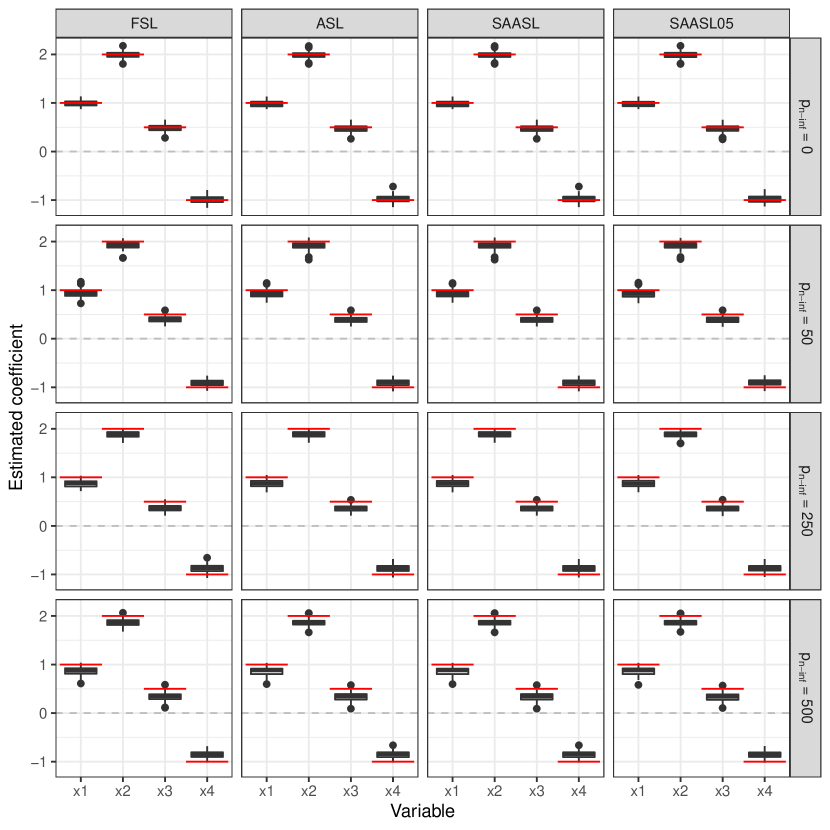
Figure B.1: Boxplot of the estimated coefficients of $\eta_{\mu}$ in 100 simulation runs. Values are taken at the stopping iterations determined by 10-folds cross-validation. The results are separated according to fixed and adaptive approaches with respect to different non-informative variables settings, i.e. $p_{\text{n-inf}}=0,50,250$ and $500$. The horizontal red lines indicate the true coefficients. The shrinkage of the coefficients towards zero can be observed from this graphic.

Figure B.2: Boxplot of the estimated coefficients of $\eta_{\sigma}$ in 100 simulation runs. Values are taken at the stopping iterations tuned by 10-folds cross-validation. The results are separated according to fixed and adaptive approaches with respect to different non-informative variables settings, i.e. $p_{\text{n-inf}}=0,50,250$ and $500$. The horizontal red lines indicate the true coefficients. The shrinkage of the coefficients towards zero can be observed from this graphic.

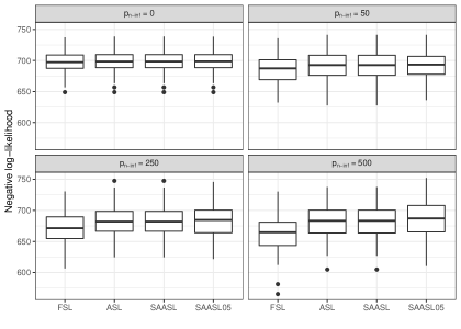
Figure B.3: Summary of the negative log-likelihood of 100 simulation runs with different estimating approaches with respect to various non-informative variables settings. Values are taken at the stopping iteration determined by 10-folds cross-validation.

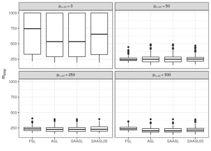
Figure B.4: $m_{\text{stop}}$ tuned by 10-fold CV with different estimating methods with respect to different non-informative variables settings. The predefined maximal learning iteration is 1000.

Appendix C Further table of section 4.2

Table C.1: The average MSE of the estimated coefficients for both model parameters $\boldsymbol{\mu}$ and $\boldsymbol{\sigma}$ w.r.t. three estimation approaches. The MSE for each coefficient is calculated not only from 100 simulation runs (Total) at their stopping iterations but also from the true positive subsets (TP), i.e., the simulations from which a coefficient is selected by all three approaches.

	$\boldsymbol{\mu}$						$\boldsymbol{\sigma}$
	$\hat{\beta}_{1}$		$\hat{\beta}_{2}$		$\hat{\beta}_{3}$		$\hat{\beta}_{1}$		$\hat{\beta}_{2}$		$\hat{\beta}_{3}$
	Total	TP	Total	TP	Total	TP	Total	TP	Total	TP	Total	TP
FSL	13.7	80.9	26.5	112.2	13.8	76.0	0.84	0.81	1.41	1.42	0.84	0.82
GAMLSS	113.8	328.8	145.6	355.8	116.8	339.4	0.82	0.79	1.44	1.44	0.81	0.79
SAASL	71.3	250.2	95.8	271.7	73.3	238.5	0.85	0.81	1.39	1.40	0.85	0.82

Appendix D Estimated coefficients of riboflavin dataset

Table D.1: The estimated coefficients of the $\boldsymbol{\mu}$-submodel with fixed and adaptive approaches. Values are taken at the $m_{\text{stop}}$ tuned by 5-folds CV.

	Variable	FSL	ASL	SAASL	SAASL05	glmnet
1	(Intercept)	-7.03	-7.04	-7.04	-7.03	0.72
2	ARGF_at	-0.08	-0.02	-0.02	-0.02
3	IOLE_at	-0.32			-0.02
4	LYSC_at					-0.06
5	RPLO_at				-0.02	-0.08
6	SPOIISA_at	0.35	0.19	0.19	0.23	0.02
7	XKDC_at	0.18			0.09	0.19
8	XKDO_at		0.02	0.02	0.03
9	XKDS_at	0.11	0.08	0.08	0.08	0.06
10	XLYA_at					0.05
11	XTMA_at		0.03	0.03	0.01
12	XTRA_at					0.01
13	YCDH_at					-0.03
14	YCGM_at	-0.09	-0.06	-0.06	-0.06	-0.01
15	YCGN_at		-0.04	-0.04	-0.04
16	YCGO_at	-0.07				-0.14
17	YCGP_at				-0.03
18	YCKE_at	0.15	0.12	0.12	0.14	0.15
19	YCLB_at	0.29
20	YCSG_at		-0.08	-0.08	-0.18
21	YDAO_at				-0.03
22	YDAR_at	-0.24	-0.16	-0.16	-0.16
23	YDDK_at					-0.04
24	YEBC_at					-0.55
25	YHAI_at		0.12	0.12	0.11
26	YHFU_at		-0.02	-0.02	-0.03	-0.01
27	YJCJ_at	0.11	0.04	0.04	0.04
28	YKBA_at					0.01
29	YKUH_at		0.05	0.05	0.06
30	YOAB_at					-0.34
31	YORB_i_at		0.03	0.03	0.05	0.10
32	YOZH_i_at		0.02	0.02
33	YPGA_at					-0.05
34	YTGB_at					-0.09
35	YWQD_at				-0.02
36	YXJA_at		-0.01	-0.01	-0.01
37	YXLC_at		-0.03	-0.03
38	YXLD_at	-0.12	-0.14	-0.14	-0.16	-0.14
39	YXLE_at	-0.06	-0.01	-0.01	-0.01

Table D.2: The estimated coefficients of $\boldsymbol{\sigma}$-submodel with fixed and adaptive approaches. Values are taken at the $m_{\text{stop}}$ tuned by 5-folds CV.

	Variables	FSL	ASL	SAASL	SAASL05
1	(Intercept)	-1.41	-1.29	-1.29	-1.53
2	COTJC_at		-0.18	-0.18
3	DEGA_at	-0.13	-0.61	-0.61	-0.89
4	EXPZ_at		0.21	0.21	0.05
5	LEVD_at	0.24	0.15	0.15	0.19
6	NTH_at	-0.09	-0.11	-0.11
7	PHRI_r_at	0.06			0.03
8	TRUA_at	-0.09	-0.74	-0.74	-0.71
9	XLYA_at	-0.06
10	XPF_at				-0.05
11	YACN_at	0.20
12	YCNK_at	0.66	0.06	0.06	0.27
13	YFIG_at	-0.08			-0.09
14	YFMD_at	-0.25	-0.43	-0.43	-0.35
15	YHBD_at		-0.21	-0.21	-0.19
16	YHEN_at				-0.05
17	YHFS_at				0.06
18	YITQ_at				-0.24
19	YJFB_at		-0.11	-0.11	-0.09
20	YKRS_at		0.29	0.29	0.35
21	YKVV_at		0.06	0.06	0.28
22	YPGA_at	0.07	0.05	0.05	0.12
23	YSBA_at		-0.55	-0.55	-0.28
24	YSBB_at	-0.15	-0.23	-0.23	-0.20
25	YTFP_at	-0.24
26	YTQI_at	0.10	0.16	0.16	0.11
27	YURR_at		-0.07	-0.07	-0.11
28	YWQA_at	-0.11			-0.20
29	YYAE_at				-0.06
30	YYBT_at	-0.08			-0.03

References

- Brent (2013) Brent, R. P. (2013). Algorithms for minimization without derivatives. Courier Corporation.
- Bühlmann (2006) Bühlmann, P. (2006, 04). Boosting for high-dimensional linear models. The Annals of Statistics 34(2), 559–583.
- Bühlmann and Hothorn (2007) Bühlmann, P. and T. Hothorn (2007, 11). Boosting algorithms: Regularization, prediction and model fitting. Statistical Science 22(4), 477–505.
- Bühlmann et al. (2014) Bühlmann, P., M. Kalisch, and L. Meier (2014). High-dimensional statistics with a view toward applications in biology. Annual Review of Statistics and Its Application 1(1), 255–278.
- Bühlmann and Yu (2003) Bühlmann, P. and B. Yu (2003). Boosting with the L2 loss. Journal of the American Statistical Association 98(462), 324–339.
- Dezeure et al. (2015) Dezeure, R., P. Bühlmann, L. Meier, and N. Meinshausen (2015). High-dimensional inference: Confidence intervals, p-values and R-software hdi. Statistical Science 30(4), 533–558.
- Fahrmeir and Kneib (2011) Fahrmeir, L. and T. Kneib (2011). Bayesian smoothing and regression for longitudinal, spatial and event history data. Oxford University Press.
- Friedman et al. (2000) Friedman, J., T. Hastie, and R. Tibshirani (2000, 04). Additive logistic regression: a statistical view of boosting (with discussion and a rejoinder by the authors). The Annals of Statistics 28(2), 337–407.
- Friedman et al. (2010) Friedman, J., T. Hastie, and R. Tibshirani (2010). Regularization paths for generalized linear models via coordinate descent. Journal of Statistical Software 33(1), 1–22.
- Friedman (2001) Friedman, J. H. (2001, 10). Greedy function approximation: A gradient boosting machine. Annals of statistics 29(5), 1189–1232.
- Hepp et al. (2016) Hepp, T., M. Schmid, O. Gefeller, E. Waldmann, and A. Mayr (2016). Approaches to regularized regression - a comparison between gradient boosting and the Lasso. Methods of information in medicine 55 5, 422–430.
- Hepp et al. (2019) Hepp, T., M. Schmid, and A. Mayr (2019). Significance tests for boosted location and scale models with linear base-learners. The International Journal of Biostatistics 15(1), 20180110.
- Hofner et al. (2015) Hofner, B., L. Boccuto, and M. Göker (2015, May). Controlling false discoveries in high-dimensional situations: boosting with stability selection. BMC Bioinformatics 16(1), 144.
- Hofner et al. (2018) Hofner, B., A. Mayr, N. Fenske, and M. Schmid (2018). gamboostLSS: Boosting Methods for GAMLSS Models. R package version 2.0-1.
- Hofner et al. (2014) Hofner, B., A. Mayr, N. Robinzonov, and M. Schmid (2014, February). Model-based boosting in R: A hands-on tutorial using the R package mboost. Computational Statistics 29(1-2), 3–35.
- Hofner et al. (2016) Hofner, B., A. Mayr, and M. Schmid (2016). gamboostlss: An R package for model building and variable selection in the gamlss framework. Journal of Statistical Software, Articles 74(1), 1–31.
- Hothorn et al. (2010) Hothorn, T., P. Buehlmann, T. Kneib, M. Schmid, and B. Hofner (2010). Model-based boosting 2.0. Journal of Machine Learning Research 11, 2109–2113.
- Hothorn et al. (2018) Hothorn, T., P. Buehlmann, T. Kneib, M. Schmid, and B. Hofner (2018). mboost: Model-Based Boosting. R package version 2.9-1.
- Hothorn et al. (2011) Hothorn, T., J. Müller, B. Schröder, T. Kneib, and R. Brandl (2011). Decomposing environmental, spatial, and spatiotemporal components of species distributions. Ecological Monographs 81(2), 329–347.
- Kohavi et al. (1995) Kohavi, R. et al. (1995). A study of cross-validation and bootstrap for accuracy estimation and model selection. Ijcai 14(2), 1137–1145.
- Mayr et al. (2012) Mayr, A., N. Fenske, B. Hofner, T. Kneib, and M. Schmid (2012). Generalized additive models for location, scale and shape for high dimensional data—a flexible approach based on boosting. Journal of the Royal Statistical Society: Series C (Applied Statistics) 61(3), 403–427.
- Meinshausen and Bühlmann (2010) Meinshausen, N. and P. Bühlmann (2010). Stability selection. Journal of the Royal Statistical Society: Series B (Statistical Methodology) 72(4), 417–473.
- Rigby and Stasinopoulos (2005) Rigby, R. A. and D. M. Stasinopoulos (2005). Generalized additive models for location, scale and shape. Journal of the Royal Statistical Society: Series C (Applied Statistics) 54(3), 507–554.
- Ripley (2004) Ripley, B. D. (2004). Selecting amongst large classes of models. Methods and Models in Statistics, 155–170.
- Stasinopoulos and Rigby (2007) Stasinopoulos, D. and R. Rigby (2007). Generalized additive models for location scale and shape (gamlss) in r. Journal of Statistical Software, Articles 23(7), 1–46.
- Stasinopoulos et al. (2017) Stasinopoulos, D., R. Rigby, G. Heller, V. Voudouris, and F. De Bastiani (2017, 03). Flexible regression and smoothing: Using GAMLSS in R. Chapman and Hall/CRC.
- Thomas et al. (2018) Thomas, J., A. Mayr, B. Bischl, M. Schmid, A. Smith, and B. Hofner (2018, May). Gradient boosting for distributional regression: faster tuning and improved variable selection via noncyclical updates. Statistics and Computing 28(3), 673–687.