Flavor Dependent $U(1)$ Symmetric Zee Model
with a Vector-like Lepton

Abstract

We extend the Zee model by introducing a vector-like lepton doublet and a flavor dependent global $U(1)$ symmetry. Flavor changing neutral currents in the quark sector can be naturally forbidden at tree level due to the $U(1)$ symmetry, while sufficient amount of lepton flavor violation is provided to explain current neutrino oscillation data. In our model, additional sources of CP-violation appear in the lepton sector, but their contribution to electric dipole moments is much smaller than current experimental bounds due to the Yukawa structure constrained by the $U(1)$ symmetry. We find that there is a parameter region where the strongly first order electroweak phase transition can be realized, which is necessary for the successful scenario of the electroweak baryogenesis in addition to new CP-violating phases. In the benchmark points satisfying neutrino data, lepton flavor violation data and the strongly first order phase transition, we show that an additional CP-even Higgs boson $H$ mainly decays into a lighter CP-odd Higgs boson $A$, i.e., $H\to AZ$ or $H\to AA$ with a characteristic pattern of lepton flavor violating decays of $A$.

I Introduction

Neutrino oscillations are the phenomena which indicate clear evidence for the necessity of physics beyond the standard model (SM). From various measurements, it has been known that masses of neutrinos have to be much smaller than those of charged fermions, e.g., ${\cal O}(10^{12})$ times smaller than the top quark mass. This strongly suggests that the neutrino mass is generated by a different mechanism from that for charged fermions, i.e., Dirac masses via Yukawa interactions with a Higgs doublet field. In such context, Majorana masses for neutrinos can be a good candidate, which are effectively described by the dimension five Weinberg operator Weinberg (1979). The question is then how the Weinberg operator can be written in terms of the ultra-violet physics. The simplest example has been known as the type-I seesaw mechanism Minkowski (1977); Yanagida (1980); Mohapatra and Senjanovic (1980), where only right-handed neutrinos are sufficient to be added to the SM. This, however, requires huge Majorana masses of the right-handed neutrinos, typically order ${\cal O}(10^{14})$ GeV assuming order one Dirac Yukawa couplings, so that direct detections for such heavy particles are quite challenging.

As an alternative direction, we can consider a scenario where neutrino masses are generated via quantum effects by which new particles are not needed to be super heavy. This idea has originally been realized in the model proposed by A. Zee Zee (1980) (Zee model), where neutrino masses are generated at one-loop level. In the Zee model, right-handed neutrinos are not introduced, while the Higgs sector is extended by adding an additional Higgs doublet and charged singlet fields, by which the lepton number is explicitly broken via scalar interactions. The Zee model predicts a characteristic structure of the mass matrix for Majorana neutrinos, e.g., all the diagonal elements to be zero. Such a strong prediction ironically turns out to kill the model itself, because of the contradiction with the observed neutrino oscillations Koide (2001); Frampton et al. (2002); He (2004). Therefore, modifications or extensions of the Zee model are inevitable.

The simplest modification would be just not imposing a $Z_{2}$ symmetry which is originally introduced to avoid tree level flavor changing neutral currents (FCNCs) mediated by neutral Higgs bosons. In this case, both Higgs doublet fields can couple to each type of fermions, i.e., up-type quarks, down-type quarks and charged leptons, so that we obtain sufficient sources of lepton flavor violations in order to explain current neutrino data He (2004); Aristizabal Sierra and Restrepo (2006); He and Majee (2012); Herrero-García et al. (2017). However, this requires unnatural fine-tunings in the quark sector to avoid various constraints from flavor changing processes such as the $B$-$\bar{B}$ mixing. Recently, in Ref. Nomura and Yagyu (2019) another possibility has been proposed, where a global $U(1)^{\prime}$ symmetry is introduced instead of the $Z_{2}$ symmetry. Taking flavor dependent charge assignments for lepton fields, we can obtain additional sources of lepton flavor violations, and at the same time matrices for quark Yukawa interactions are diagonal.

In this paper, we clarify that the minimal Zee model with the $U(1)^{\prime}$ symmetry cannot explain current neutrino oscillation data. We thus add a vector-like lepton doublet, as one of the simplest extensions, to the model, in which we assume a weak mixing between the new vector-like field and the SM leptons to avoid large contributions to charged lepton flavor violating (CLFV) decays. In this extension, an anti-symmetric Yukawa matrix among the lepton doublets and the charged singlet scalar becomes a $4\times 4$ form including six independent complex parameters which can be analytically solved in terms of the neutrino parameters driven by experiments. This extended model also provides new sources of CP-violation in the lepton sector, which is well motivated for the explanation of baryon asymmetry of Universe Sakharov (1991). Interestingly, it is clarified that effects of the CP-violating phases on the electron electric dipole moment (EDM) are negligibly small because of the structure of the Yukawa matrices constrained by the $U(1)^{\prime}$ symmetry. We then study the electroweak phase transition, and find a region of the parameter space where the strongly first order phase transition (FOPT) is realized which is needed for the successful scenario of the electroweak baryogenesis Kuzmin et al. (1985); Shaposhnikov (1987). In addition, we discuss collider signatures of our model, particularly focusing on Higgs boson decays into a flavor violating lepton pair in the benchmark parameter points which satisfy neutrino data, CLFV data and the strongly FOPT.

This paper is organized as follows. In Sec. II, we define our model, and give the Yukawa interaction terms and the Higgs potential. Constraints from perturbative unitarity and vacuum stability are also discussed. In Sec. III, we discuss neutrino masses which are generated at one-loop level, and numerically show the necessity of the extension of the minimal Zee model in order to reproduce the current neutrino oscillation data. Sec. IV is devoted for the discussion of various constraints from flavor experiments such as the electron EDM and CLFV decays. Collider phenomenologies are then discussed in Sec. V, particularly focusing on production and decay of additional neutral Higgs bosons at the LHC. In Sec. VI, we show the electroweak phase transition as a cosmological consequences in our model. Conclusions are given in Sec. VII. In Appendix, we give the approximate formulae for each element of the anti-symmetric matrix $F$ (Appendix A), explicit expressions for the amplitude of the CLFV decays (Appendix B) and those for the effective potential at finite temperature (Appendix C).

II Model

We briefly review the Zee model with a global $U(1)^{\prime}$ symmetry which has been proposed in Ref. Nomura and Yagyu (2019). The content of the scalar sector is the same as the original Zee model, which is composed of two isospin doublet fields $\Phi_{1}$ and $\Phi_{2}$ and a pair of singly-charged scalar singlets $S^{\pm}$. This model, however, cannot explain current neutrino oscillation data, as it will be shown in the next section. One of the simplest extensions is the introduction of a vector-like lepton doublet $L^{4}\equiv(\nu_{T},T^{-})^{T}$ to the model. In this section, we first discuss Yukawa interactions with $L^{4}$, and then consider the Higgs potential.

II.1 Yukawa Interactions

The most general form of the Lagrangian for the lepton sector is given by

$$\mathcal{L}_{\rm lep} =-M^{\prime}\bar{L}^{4}L^{4}-\left[\bar{L}_{L}^{A}(\tilde{Y}_{1})^{AB}\Phi_{1}\ell_{R}^{B}+\bar{L}_{L}^{A}(\tilde{Y}_{2})^{AB}\Phi_{2}\ell_{R}^{B}+\overline{L_{L}^{cA}}(\tilde{F})^{AB}(i\tau_{2})L_{L}^{B}S^{+}+\text{h.c.}\right],$$ (1)

where $L_{L}$ $(\ell_{R})$ are the left-handed (right-handed) lepton fields. The indices $A$ and $B$ ($=1,\dots,4$) represent the flavor with $L_{L}^{1\text{--}3}$ and $\ell_{R}^{1\text{--}3}$ to be identified with the SM lepton fields, and $\ell_{R}^{4}\equiv T_{R}$ which is the charged component of $L_{R}^{4}$. The supscript $c$ denotes the charge conjugation. The structure of the Yukawa matrices $\tilde{Y}_{1}$ and $\tilde{Y}_{2}$ is constrained by the $U(1)^{\prime}$ symmetry depending on its charge assignment. Throughout the paper, we take the Class-I assignment defined in Ref. Nomura and Yagyu (2019), where $\Phi_{1}$ and the right-handed tau lepton $\tau_{R}$ are charged with $q(\neq 0)$ and $-q$, respectively, while all the other fields are neutral.  This assignment provides the largest number of non-zero elements of Yukawa interaction matrices given as follows:

$$\tilde{Y}_{1}=\begin{pmatrix}0&0&\times&0\\ 0&0&\times&0\\ 0&0&\times&0\\ 0&0&\times&0\end{pmatrix},~{}~{}\tilde{Y}_{2}=\begin{pmatrix}\times&\times&0&0\\ \times&\times&0&0\\ \times&\times&0&0\\ \times&\times&0&0\end{pmatrix},$$ (2)

where $\times$ denotes a non-zero complex value. The fourth column has to be zero due to the gauge invariance. The matrix $\tilde{F}$ is the anti-symmetric $4\times 4$ form, so that it is described by six independent parameters. We note that Yukawa interaction terms for quarks are the same form as those in the SM, where only $\Phi_{2}$ couples to quarks due to the $U(1)^{\prime}$ symmetry. Thus, FCNCs do not appear in the quark sector at tree level.

In order to separately write fermion mass terms and interaction terms, we introduce the Higgs basis Georgi and Nanopoulos (1979); Donoghue and Li (1979) defined as

$$\begin{pmatrix}\Phi_{1}\\ \Phi_{2}\end{pmatrix}=\begin{pmatrix}c_{\beta}&-s_{\beta}\\ s_{\beta}&c_{\beta}\end{pmatrix}\begin{pmatrix}\Phi\\ \Phi^{\prime}\end{pmatrix},$$ (3)

where we introduced shorthand notation for the trigonometric functions as $s_{X}=\sin X$ and $c_{X}=\cos X$. In addition, we defined $\tan\beta=\langle\Phi_{2}^{0}\rangle/\langle\Phi_{1}^{0}\rangle$ and

$$\Phi=\begin{pmatrix}G^{+}\\ \frac{h_{1}^{\prime}+v+iG^{0}}{\sqrt{2}}\end{pmatrix},\quad\Phi^{\prime}=\begin{pmatrix}H^{+}\\ \frac{h_{2}^{\prime}+iA}{\sqrt{2}}\end{pmatrix}.$$ (4)

In Eq. (4), $G^{\pm}$ and $G^{0}$ are the Nambu-Goldstone (NG) bosons which are absorbed into the longitudinal components of $W^{\pm}$ and $Z$ bosons, respectively, while $H^{\pm}$, $h_{1,2}^{\prime}$ and $A$ are physical charged, CP-even and CP-odd Higgs bosons, respectively. The VEV $v$ is related to the Fermi constant $G_{F}$ by $v=(\sqrt{2}G_{F})^{-1/2}\simeq 246$ GeV. In general, $h_{1}^{\prime}$ $(H^{\pm})$ can mix with $h_{2}^{\prime}$ ($S^{\pm}$). Their mass eigenstates are defined as

$$\begin{pmatrix}h_{1}^{\prime}\\ h_{2}^{\prime}\end{pmatrix} =\begin{pmatrix}c_{\alpha-\beta}&-s_{\alpha-\beta}\\ s_{\alpha-\beta}&c_{\alpha-\beta}\end{pmatrix}\begin{pmatrix}H\\ h\end{pmatrix},\quad\begin{pmatrix}H^{\pm}\\ S^{\pm}\end{pmatrix}=\begin{pmatrix}c_{\chi}&-s_{\chi}\\ s_{\chi}&c_{\chi}\end{pmatrix}\begin{pmatrix}H_{1}^{\pm}\\ H_{2}^{\pm}\end{pmatrix},$$ (5)

where the mixing angles $\alpha$ and $\chi$ are expressed in terms of the parameters in the Higgs potential, see Eq. (38). We identify $h$ with the discovered Higgs boson with a mass of about 125 GeV.

In the Higgs basis, Eq. (1) is rewritten as

$$\mathcal{L}_{\rm lep} =-M^{\prime}\bar{L}^{4}L^{4}-\left[\bar{L}_{L}^{A}\left(\tilde{Y}_{\Phi}^{AB}\Phi+\tilde{Y}_{\Phi^{\prime}}^{AB}\Phi^{\prime}\right)\ell_{R}^{B}+\overline{L_{L}^{cA}}\tilde{F}^{AB}(i\tau_{2})L_{L}^{B}S^{+}+\text{h.c.}\right],$$ (6)

where

$$\tilde{Y}_{\Phi}=\tilde{Y}_{1}c_{\beta}+\tilde{Y}_{2}s_{\beta},\quad\tilde{Y}_{\Phi^{\prime}}=-\tilde{Y}_{1}s_{\beta}+\tilde{Y}_{2}c_{\beta}.$$ (7)

The mass matrix for the charged leptons is expressed by

$$\tilde{M}_{\ell}=\begin{pmatrix}\frac{v}{\sqrt{2}}\tilde{Y}_{\Phi}^{ab}&0\\ \frac{v}{\sqrt{2}}\tilde{Y}_{\Phi}^{4b}&M^{\prime}\end{pmatrix},\quad(a,b=1,\dots,3).$$ (8)

This matrix can be diagonalized by the unitary rotations $L_{L}=V_{L}L_{L}^{\prime}$ and $\ell_{R}=V_{R}\ell_{R}^{\prime}$ such that

$$M_{\ell}\equiv\text{diag}(m_{e},m_{\mu},m_{\tau},m_{T})=V_{L}^{\dagger}\tilde{M}_{\ell}V_{R}.$$ (9)

The interaction terms are then extracted in the mass eigenstates of the Higgs bosons and the charged fermions as

$$\mathcal{L}_{\rm lep}^{\rm int} =-\frac{1}{\sqrt{2}}\bar{\ell}^{\prime}\left[(s_{\beta-\alpha}Y_{\Phi}+c_{\beta-\alpha}Y_{\Phi^{\prime}})h+(c_{\beta-\alpha}Y_{\Phi}-s_{\beta-\alpha}Y_{\Phi^{\prime}})H+iY_{\Phi^{\prime}}A\right]P_{R}\ell^{\prime}+\text{h.c.}$$

$$-(2s_{\chi}\overline{\nu^{\prime c}}FP_{L}+c_{\chi}\bar{\nu}^{\prime}Y_{\Phi^{\prime}}P_{R})\ell^{\prime}\,H_{1}^{+}-(2c_{\chi}\overline{\nu^{\prime c}}FP_{L}-s_{\chi}\bar{\nu}^{\prime}Y_{\Phi^{\prime}}P_{R})\ell^{\prime}\,H_{2}^{+}+\text{h.c.},$$ (10)

where $P_{L}$ ($P_{R}$) is the projection operator for the left (right) handed fermions, and

$$Y_{\Phi} =V_{L}^{\dagger}\tilde{Y}_{\Phi}V_{R},\quad Y_{\Phi^{\prime}}=V_{L}^{\dagger}\tilde{Y}_{\Phi^{\prime}}V_{R},\quad F=V_{L}^{T}\tilde{F}V_{L}.$$ (11)

These Yukawa matrices can be rewritten by using Eq. (9) as,

$$Y_{\Phi}=\frac{\sqrt{2}}{v}M_{\ell}V_{R}^{\dagger}P_{123}V_{R},\quad Y_{\Phi^{\prime}}=\frac{\sqrt{2}}{v}M_{\ell}V_{R}^{\dagger}P_{\beta}V_{R},$$ (12)

where $P_{123}\equiv\text{diag}(1,1,1,0)$ and $P_{\beta}\equiv\text{diag}(\cot\beta,\cot\beta,-\tan\beta,0)$. We note that $V_{L}$ does not appear in the above expression due to its unitarity.

In general, the matrices $Y_{\Phi}$ and $Y_{\Phi^{\prime}}$ contain non-zero off-diagonal elements which can introduce large effects on CLFV decays mediated by scalar bosons. In order to avoid such CLFV decays, we assume that the fourth lepton doublet $L^{4}$ is weakly mixed with three generations of the SM leptons. This can naturally be realized by taking the mass parameter $M^{\prime}$ to be much larger than charged lepton masses, e.g., the tau lepton mass.

Let us clarify how the interaction matrices defined above can be expressed in the weak mixing scenario. First, the unitary matrices $V_{R}$ can be expressed as

$$V_{R} =V_{23}(\alpha_{23},\varphi_{23})V_{13}(\alpha_{13},\varphi_{13})V_{12}(\alpha_{12},\varphi_{12})V_{14}(\alpha_{14},\varphi_{14})V_{24}(\alpha_{24},\varphi_{24})V_{34}(\alpha_{34},\varphi_{34}),$$ (13)

where $V_{ij}$ are the $4\times 4$ unitary matrices with $i$–$i$ and $j$–$j$ elements to be $\cos\alpha_{ij}$ and $i$–$j$ ($j$–$i$) to be $\sin\alpha_{ij}e^{-i\varphi_{ij}}$ ($-\sin\alpha_{ij}e^{i\varphi_{ij}}$), while all the other diagonal (off-diagonal) elements to be unity (zero). Second, the weak mixing scenario indicates that the mixing angles $\alpha_{a4}$ $(a=1,2,3)$ are small, so that we reparametrize them as $\alpha_{a4}\to\epsilon\alpha_{a4}$ with $\epsilon\ll 1$. In this case, the unitary matrices can be expressed as,

$$V_{R} =V_{R,0}+\delta V_{R},$$ (14)

where $V_{R,0}$ is given by taking $\epsilon\to 0$ in $V_{R}$, while $\delta V_{R}$ is

$$\delta V_{R}=\left(\begin{array}[]{c|c}{\cal O}(\epsilon^{2})&{\cal O}(\epsilon)\\ \hline\cr{\cal O}(\epsilon)&{\cal O}(\epsilon^{2})\end{array}\right),$$ (17)

with the upper-left (lower-right) block being the $3\times 3$ ($1\times 1$) form. Third, using this expansion, the Yukawa matrices $Y_{\Phi}$ and $Y_{\Phi^{\prime}}$ are expressed as

$$Y_{\Phi}=Y_{\Phi,0}+\delta Y_{\Phi},\quad Y_{\Phi^{\prime}}=Y_{\Phi^{\prime},0}+\delta Y_{\Phi^{\prime}},$$ (18)

where

$$Y_{\Phi^{\prime},0} =\frac{\sqrt{2}}{v}\left(\begin{array}[]{c|c}M_{\ell}^{3\times 3}(V_{R,0}^{3\times 3})^{\dagger}P_{\beta}^{3\times 3}V_{R,0}^{3\times 3}&0\\ \hline\cr 0&0\end{array}\right),$$ (21)

$$\delta Y_{\Phi^{\prime}} =\frac{\sqrt{2}}{v}\left(\begin{array}[]{c|c}\epsilon^{2}M_{\ell}^{3\times 3}[(\delta V_{R}^{3\times 3})^{\dagger}P_{\beta}^{3\times 3}V_{R,0}^{3\times 3}+\text{h.c.}]&\epsilon M_{\ell}^{3\times 3}(V_{R,0}^{3\times 3})^{\dagger}P_{\beta}^{3\times 3}\delta V_{R}^{3\times 1}\\ \hline\cr\epsilon m_{T}(\delta V_{R}^{3\times 1})^{\dagger}P_{\beta}^{3\times 3}V_{R,0}^{3\times 3}&\epsilon^{2}m_{T}(\delta V_{R}^{3\times 1})^{\dagger}P_{\beta}^{3\times 3}(\delta V_{R}^{3\times 1})\end{array}\right)+{\cal O}(\epsilon^{3}),$$ (24)

with $X^{3\times 3}$ ($X^{3\times 1}$) being the $3\times 3$ $(3\times 1)$ part of a $4\times 4$ matrix $X$. The expressions for $Y_{\Phi,0}$ and $\delta Y_{\Phi}$ are given by replacing $P_{\beta}^{3\times 3}\to I^{3\times 3}$ in $Y_{\Phi^{\prime},0}$ and $\delta Y_{\Phi^{\prime}}$, respectively. We can see that the bottom-left block ($1\times 3$ part) of $\delta Y_{\Phi}$ and $\delta Y_{\Phi^{\prime}}$ can be ${\cal O}(1)$ for $\epsilon\sim 1$ because of the dependence of $m_{T}$, and this effect can enter in the CLFV decays, e.g., $\ell\to\ell^{\prime}\gamma$ decays via the fourth lepton loops. Thus, the weak mixing scenario, $\epsilon\ll 1$, is essentially important to avoid such a large effect, as amplitudes for the CLFV decay are highly suppressed by $\epsilon^{2}$. Detailed discussions for constraints from the CLFV decays will be given in Sec. IV. Interestingly, the mixing effect on masses of active neutrinos is not suppressed by $\epsilon^{2}$, but $\epsilon$ as it will be explained in the next section. It is also important to mention here that $F$, $\delta Y_{\Phi}$ and $\delta Y_{\Phi^{\prime}}$ can be complex, so that they can provide new sources of CP-violation, and their effects on EDMs will be discussed in Sec. IV.

It is clear that in the $\epsilon\to 0$ limit, $Y_{\Phi}$ becomes diagonal, while $Y_{\Phi^{\prime}}$ takes the block diagonal form as shown in Eq. (21). Furthermore, in the scenario with a softly-broken $Z_{2}$ symmetry, the matrix $Y_{\Phi^{\prime}}$ also becomes proportional to the diagonalized mass matrix as in the two Higgs doublet models (THDMs):

$$Y_{\Phi^{\prime}}\xrightarrow[Z_{2}]{}\frac{\sqrt{2}M_{\ell}}{v}\zeta,$$ (25)

where $\zeta=\cot\beta$ ($-\tan\beta$) for the Type-I and Type-Y (Type-II and Type-X) THDM Aoki et al. (2009).

II.2 Higgs Potential

The most general Higgs potential is given by

$$V =m_{1}^{2}|\Phi_{1}|^{2}+m_{2}^{2}|\Phi_{2}|^{2}-m_{3}^{2}(\Phi_{1}^{\dagger}\Phi_{2}+\text{h.c.})+m_{S}^{2}|S^{+}|^{2}+\mu[\Phi_{1}^{T}(i\tau_{2})\Phi_{2}(S^{+})^{*}+\text{h.c.}]$$

$$+\frac{\lambda_{1}}{2}|\Phi_{1}|^{4}+\frac{\lambda_{2}}{2}|\Phi_{2}|^{4}+\lambda_{3}|\Phi_{1}|^{2}|\Phi_{2}|^{2}+\lambda_{4}|\Phi_{1}^{\dagger}\Phi_{2}|^{2}$$

$$+\sigma_{1}|S^{+}|^{2}|\Phi_{1}|^{2}+\sigma_{2}|S^{+}|^{2}|\Phi_{2}|^{2}+\frac{\sigma_{3}}{2}|S^{+}|^{4}.$$ (26)

In the above expression, $m_{3}^{2}$ and $\mu$ terms softly break the $U(1)^{\prime}$ symmetry, and their complex phases are removed by using the phase redefinition of the scalar fields without the loss of generality. Thus, there is no CP-violating phase in the Higgs potential. We note that the $(\Phi_{1}^{\dagger}\Phi_{2})^{2}$ term is forbidden because of the $U(1)^{\prime}$ symmetry. Thus, a pseudo-NG boson, corresponding to $A$, appears due to the spontaneous breaking of the $U(1)^{\prime}$ symmetry. The $\mu$ term plays a crucial role for the neutrino mass generation, as this term breaks two units of the lepton number when we assign the lepton number of $(\Phi_{1},\Phi_{2},S^{\pm})$ to be $(0,0,\pm 2)$.

After imposing the tadpole conditions for two CP-even Higgs bosons, all the masses of the physical Higgs bosons are expressed as

$$m_{A}^{2} =\frac{m_{3}^{2}}{s_{\beta}c_{\beta}},$$ (27)

$$m_{H}^{2} =(M_{\text{even}}^{2})_{11}^{2}\,c^{2}_{\beta-\alpha}+(M_{\text{even}}^{2})_{22}^{2}\,s^{2}_{\beta-\alpha}-(M_{\text{even}}^{2})_{12}^{2}\,s_{2(\beta-\alpha)},$$ (28)

$$m_{h}^{2} =(M_{\text{even}}^{2})_{11}\,s^{2}_{\beta-\alpha}+(M_{\text{even}}^{2})_{22}c^{2}_{\beta-\alpha}+(M_{\text{even}}^{2})_{12}s_{2(\beta-\alpha)},$$ (29)

$$m_{H_{1}^{\pm}}^{2} =(M_{\pm}^{2})_{11}\,c^{2}_{\chi}+(M_{\pm}^{2})_{22}\,s^{2}_{\chi}+(M_{\pm}^{2})_{12}\,s_{2\chi},$$ (30)

$$m_{H_{2}^{\pm}}^{2} =(M_{\pm}^{2})_{11}\,s^{2}_{\chi}+(M_{\pm}^{2})_{22}\,c^{2}_{\chi}-(M_{\pm}^{2})_{12}\,s_{2\chi},$$ (31)

where $(M_{\text{even}}^{2})_{ij}$ and $(M_{\pm}^{2})_{ij}$ ($i,j=1,2$) are the elements of the squared mass matrices for the CP-even and singly-charged Higgs bosons in the basis of $(h_{1}^{\prime},h_{2}^{\prime})$ and $(H^{\pm},S^{\pm})$, respectively. Each element is given as

$$(M_{\text{even}}^{2})_{11} =v^{2}\left(\lambda_{1}c^{4}_{\beta}+\lambda_{2}s^{4}_{\beta}+\frac{\lambda_{3}+\lambda_{4}}{2}s^{2}_{2\beta}\right),$$ (32)

$$(M_{\text{even}}^{2})_{22} =m_{A}^{2}+\frac{v^{2}}{8}[\lambda_{1}+\lambda_{2}-2(\lambda_{3}+\lambda_{4})](1-c_{4\beta}),$$ (33)

$$(M_{\text{even}}^{2})_{12} =\frac{v^{2}}{2}[-\lambda_{1}c^{2}_{\beta}+\lambda_{2}s^{2}_{\beta}+(\lambda_{3}+\lambda_{4})c_{2\beta}]s_{2\beta},$$ (34)

$$(M_{\pm}^{2})_{11} =m_{A}^{2}-\frac{v^{2}}{2}\lambda_{4},$$ (35)

$$(M_{\pm}^{2})_{22} =m_{S}^{2}+\frac{v^{2}}{2}(\sigma_{1}c^{2}_{\beta}+\sigma_{2}s^{2}_{\beta}),$$ (36)

$$(M_{\pm}^{2})_{12} =-v\frac{\mu}{\sqrt{2}}.$$ (37)

The mixing angles are expressed in terms of these matrix elements:

$$\tan 2(\alpha-\beta) =\frac{2(M_{\text{even}}^{2})_{12}}{(M_{\text{even}}^{2})_{11}-(M_{\text{even}}^{2})_{22}},~{}\tan 2\chi=\frac{2(M_{\pm}^{2})_{12}}{(M_{\pm}^{2})_{11}-(M_{\pm}^{2})_{22}}.$$ (38)

From the above discussion, we can choose the following twelve parameters as inputs:

$$m_{h},~{}m_{A},~{}m_{H},~{}m_{H_{1}^{\pm}},~{}m_{H_{2}^{\pm}},~{}m_{S},~{}v,~{}s_{\beta-\alpha},~{}s_{\chi},~{}\tan\beta,~{}\tan\sigma,~{}\sigma_{3},$$ (39)

where $\tan\sigma\equiv\sigma_{2}/\sigma_{1}$. Among the above parameters, $v$ and $m_{h}$ are fixed to be about 246 GeV and 125 GeV by experiments, respectively, and $\sigma_{3}$ is not relevant to the following discussion.

The parameters of the Higgs potential are constrained by considering bounds from perturbative unitarity and vacuum stability. In Refs. Muhlleitner et al. (2017); Chen et al. (2020), all the independent eigenvalues of the $s$-wave amplitude matrix for 2 body to 2 body elastic scatterings ($a_{i}$) have been given in the high energy limit. Requiring $|a_{i}|\leq 1/2$, the unitarity bound is expressed in our notation as

$$\left|\frac{1}{2}\left(\lambda_{1}+\lambda_{2}+\sqrt{\left(\lambda_{1}-\lambda_{2}\right)^{2}+4\lambda_{4}^{2}}\right)\right|<8\pi,$$

$$|\lambda_{1,2,3},\sigma_{1,2}|<8\pi,\quad\left|\lambda_{3}+2\lambda_{4}\right|<8\pi,\quad\left|\lambda_{3}\pm\lambda_{4}\right|<8\pi,\quad|x_{1,2,3}|<8\pi,$$ (40)

where $x_{1,2,3}$ are the eigenvalues for the following $3\times 3$ matrix

$$\begin{pmatrix}3\lambda_{1}&2\lambda_{3}+\lambda_{4}&\sqrt{2}\sigma_{1}\\ 2\lambda_{3}+\lambda_{4}&3\lambda_{2}&\sqrt{2}\sigma_{2}\\ \sqrt{2}\sigma_{1}&\sqrt{2}\sigma_{2}&2\sigma_{3}\end{pmatrix}.$$ (41)

The vacuum stability of the potential has also been discussed in Refs. Kanemura et al. (2001); Muhlleitner et al. (2017). Requiring the potential bounded from below in any direction with large scalar field values, the parameters in the Higgs potential are constrained to be within the following domain Muhlleitner et al. (2017)

$$\Omega_{1}\cup\Omega_{2},$$ (42)

where

$$\Omega_{1}=\Big{\{}\lambda_{1},\lambda_{2},\sigma_{3}>0;\sqrt{\lambda_{1}\sigma_{3}}+\sigma_{1}>0;\sqrt{\lambda_{2}\sigma_{3}}+\sigma_{2}>0;$$

$$\qquad\qquad\sqrt{\lambda_{1}\lambda_{2}}+\lambda_{3}+D>0;\sigma_{1}+\sqrt{\frac{\lambda_{1}}{\lambda_{2}}}\sigma_{2}\geq 0\Big{\}},$$ (43)

$$\Omega_{2}=\Big{\{}\lambda_{1},\lambda_{2},\sigma_{3}>0;\sqrt{\lambda_{2}\sigma_{3}}\geq\sigma_{2}>-\sqrt{\lambda_{2}\sigma_{3}};\sqrt{\lambda_{1}\sigma_{3}}>-\sigma_{1}\geq\sqrt{\frac{\lambda_{1}}{\lambda_{2}}}\sigma_{2};$$

$$\qquad\qquad\sqrt{\left(\sigma_{1}^{2}-\lambda_{1}\sigma_{3}\right)\left(\sigma_{2}^{2}-\lambda_{2}\sigma_{3}\right)}>\sigma_{1}\sigma_{2}-\left(D+\lambda_{3}\right)\sigma_{3}\Big{\}},$$ (44)

with $D=\min(0,\lambda_{4})$.

III Neutrino masses

Majorana masses for the active neutrinos are generated at one-loop level. In the $\nu_{L}^{\prime}(=V_{L}\nu_{L})$ basis, we obtain the mass matrix as

$$m_{\nu}^{ab}=(FM_{\ell}C_{\rm diag}Y_{\Phi^{\prime}}^{\dagger})^{ab}+\text{transpose},~{}~{}~{}(a,b=1,\dots,3)$$ (45)

where $C_{\rm diag}$ is the diagonal matrix given by

$$C_{\rm diag}^{A}=\frac{s_{2\chi}}{32\pi^{2}}\left[\ln\frac{m_{H_{2}^{\pm}}}{m_{H_{1}^{\pm}}}+\frac{(m_{\ell}^{A})^{2}+m_{H_{1}^{\pm}}^{2}}{(m_{\ell}^{A})^{2}-m_{H_{1}^{\pm}}^{2}}\ln\frac{m_{H_{1}^{\pm}}}{m_{\ell}^{A}}-\frac{(m_{\ell}^{A})^{2}+m_{H_{2}^{\pm}}^{2}}{(m_{\ell}^{A})^{2}-m_{H_{2}^{\pm}}^{2}}\ln\frac{m_{H_{2}^{\pm}}}{m_{\ell}^{A}}\right],$$ (46)

with $m_{\ell}^{A}$ being the charged lepton mass. For $m_{\ell}^{A}\ll m_{H_{1}^{\pm}},m_{H_{2}^{\pm}}$,

$$C_{\rm diag}^{A}\simeq\frac{s_{2\chi}}{32\pi^{2}}\ln\frac{m_{H_{2}^{\pm}}^{2}}{m_{H_{1}^{\pm}}^{2}}=:C_{\rm diag}^{0}.$$ (47)

We note that the mass of the sterile neutrino $\nu_{T}$ is simply given by the vector-like mass $M^{\prime}$.

In the weak mixing scenario, the neutrino mass matrix can be expressed as

$$m_{\nu}=m_{\nu}^{0}+\epsilon m_{\nu}^{1}+\epsilon^{2}m_{\nu}^{2}+{\cal O}(\epsilon^{3}),$$ (48)

where

$$m_{\nu}^{0} =C_{\rm diag}^{0}F^{3\times 3}M_{\ell}^{3\times 3}(Y_{\Phi^{\prime},0}^{3\times 3})^{\dagger}+\text{transpose},$$ (49)

$$m_{\nu}^{1} =m_{T}C_{\rm diag}^{4}F^{3\times 1}(\delta Y_{\Phi^{\prime}}^{3\times 1}|_{\epsilon\to 1})^{\dagger}+\text{transpose},$$ (50)

$$m_{\nu}^{2} =C_{\rm diag}^{0}F^{3\times 3}M_{\ell}^{3\times 3}(\delta Y_{\Phi^{\prime}}^{3\times 3}|_{\epsilon\to 1})^{\dagger}+\text{transpose}.$$ (51)

We note that the contribution from the order $\epsilon^{2}$ term $m_{\nu}^{2}$ is much smaller than that from $m_{\nu}^{1}$ due to not only the suppression of the $\epsilon$ factor but also no enhancement by the large lepton mass $m_{T}$. Therefore, the neutrino masses can be well approximated by considering the term up to $m_{\nu}^{1}$. The neutrino mass matrix becomes the one given in the original Zee model by taking $\epsilon\to 0$ and $P_{\beta}^{3\times 3}\to\cot\beta I^{3\times 3}$ in $Y_{\Phi^{\prime},0}$, which is consistent with the expression given in Ref. He (2004);

$$m_{\nu}\to m_{\nu}^{0}=\frac{\sqrt{2}s_{2\chi}}{32\pi^{2}v}\cot\beta\ln\left(\frac{m_{H_{2}^{\pm}}^{2}}{m_{H_{1}^{\pm}}^{2}}\right)[F^{3\times 3}(M_{\ell}^{3\times 3})^{2}-(M_{\ell}^{3\times 3})^{2}F^{3\times 3}].$$ (52)

As aforementioned, this structure cannot accommodate current neutrino oscillation data.

The neutrino mass matrix can be diagonalized by introducing the PMNS matrix $U_{\rm PMNS}$ as follows:

$$U^{T}_{\rm PMNS}\,m_{\nu}\,U_{\rm PMNS}=m_{\nu}^{\rm diag}=\text{diag}(m_{1},m_{2},m_{3}),$$ (53)

where $m_{i}$ ($i=1,2,3$) are the mass eigenvalues. For the normal ordering (NO) and the inverted ordering (IO) cases, these are $m_{1}\lesssim m_{2}\ll m_{3}$ and $m_{3}\ll m_{1}\lesssim m_{2}$, respectively. The matrix $U_{\rm PMNS}$ can be parameterized as,

$$U_{\rm PMNS}\equiv\begin{pmatrix}1&0&0\\ 0&c_{\theta_{23}}&s_{\theta_{23}}\\ 0&-s_{\theta_{23}}&c_{\theta_{23}}\end{pmatrix}\begin{pmatrix}c_{\theta_{13}}&0&s_{\theta_{13}}e^{-i\delta_{\rm CPV}}\\ 0&1&0\\ -s_{\theta_{13}}e^{i\delta_{\rm CPV}}&0&c_{\theta_{13}}\end{pmatrix}\begin{pmatrix}c_{\theta_{12}}&s_{\theta_{12}}&0\\ -s_{\theta_{12}}&c_{\theta_{12}}&0\\ 0&0&1\end{pmatrix}\begin{pmatrix}e^{i\varphi_{1}}&0&0\\ 0&e^{i\varphi_{2}}&0\\ 0&0&1\end{pmatrix},$$ (54)

where $\delta_{\rm CPV}$ is the Dirac CP-phase, and $\varphi_{1,2}$ are the Majorana phases. From Eqs. (48) and (53), we obtain

$$m_{\nu}\simeq m_{\nu}^{0}+\epsilon m_{\nu}^{1}=U_{\rm PMNS}^{*}\,m_{\nu}^{\rm diag}\,U_{\rm PMNS}^{\dagger}.$$ (55)

By solving this equation, the elements of $F$ are expressed in terms of the following model parameters:

$$\alpha_{AB},~{}~{}\varphi_{AB},~{}~{}\tan\beta,~{}~{}\epsilon,~{}~{}m_{T},~{}~{}m_{H_{1,2}^{\pm}},~{}~{}s_{\chi},$$ (56)

with $\{\alpha_{AB}\}=\{\alpha_{12},~{}\alpha_{13},~{}\alpha_{23},~{}\alpha_{14},~{}\alpha_{24},~{}\alpha_{34}\}$ (similarly to $\varphi_{AB}$), and the neutrino parameters appearing in the right-hand side of Eq. (55):

$$\theta_{12},~{}~{}\theta_{23},~{}~{}\theta_{13},~{}~{}\Delta m_{\text{sol}}^{2},~{}~{}|\Delta m_{\text{atm}}^{2}|,~{}~{}m_{0},~{}~{}\delta_{\rm CPV},~{}~{}\varphi_{1,2},$$ (57)

with $m_{0}$ being the smallest eigenvalue of the neutrino masses. We define the two squared mass differences as $\Delta m_{\rm sol}^{2}\equiv m_{2}^{2}-m_{1}^{2}$ and $\Delta m_{\rm atm}^{2}\equiv|m_{3}^{2}-m_{1}^{2}|~{}~{}(|m_{3}^{2}-m_{2}^{2}|)$ for the NO (IO) case.

Now, we can reproduce the neutrino parameters shown in Eq. (57) for each fixed value of the model parameters given in Eq. (56). Typical order of the elements of $F$ can be estimated for $\tan\beta\simeq 1$ as follows:

$$F^{AB}\simeq\frac{1}{C_{\rm diag}^{B}}\frac{v}{m_{\ell}^{A}}\frac{m_{\nu}}{m_{\ell}^{B}}[1+(\epsilon^{-1}-1)\delta^{4B}]~{}~{}(\text{for}~{}~{}A<B),$$ (58)

where $m_{\nu}$ is the typical value of the elements of the neutrino mass matrix, i.e., $m_{\nu}={\cal O}(10^{-3}\text{--}10^{-2})$ eV. In Appendix A, we present better approximated formulae for these elements.

Let us comment on the case without the mixing between $L^{4}$ and the SM leptons, i.e., $\epsilon=0$ (or equivalently taking $M^{\prime}\to\infty$). In this case, we have $C_{\rm diag}^{0}$, $\tan\beta$, $F^{ab}$, $\alpha_{ab}$ and $\varphi_{ab}$ with $(a,b)=(1,2),~{}(2,3)$ and $(1,3)$ as the free input parameters, among which $C_{\rm diag}^{0}$ can be chosen to satisfy one of the measured values of the squared mass differences. By scanning the parameters within the following regions: $0\leq|F^{ab}|\leq 1$, $-\pi\leq\{\text{Arg}[F^{ab}],~{}\alpha_{ab},~{}\varphi_{ab}\}\leq\pi$ and $1\leq\tan\beta\leq 10$, we obtain $27^{\circ}\lesssim\theta_{13}\lesssim 35^{\circ}$ and $2.6\times 10^{-4}$ eV${}^{2}\lesssim\Delta m_{21}^{2}\lesssim 2.5\times 10^{-3}$ eV² in the NO case under the requirement that $\theta_{12}$, $\theta_{23}$ and $|\Delta m_{\rm atm}^{2}|$ are given within the $3\sigma$ region of the global fit results Esteban et al. (2020); NuFIT 5.0 (2020). For the IO case, we obtain $40^{\circ}\lesssim\theta_{12}\lesssim 45^{\circ}$ and $1.5\times 10^{-4}$ eV${}^{2}\lesssim\Delta m_{21}^{2}\lesssim 1.6\times 10^{-3}$ eV² under the requirement that $\theta_{23}$, $\theta_{13}$ and $|\Delta m_{\rm atm}^{2}|$ are given within the $3\sigma$ region of the global fit results. Esteban et al. (2020); NuFIT 5.0 (2020). Therefore, we clarify that the minimal model without the vector-like lepton cannot accommodate the current neutrino data.

IV Flavor Constraints

IV.1 Electric Dipole Moments

As we have discussed in the previous section, non-zero CP-violating phases appear in the lepton sector. In this subsection, we study effects of these phases on EDMs, particularly the electron EDM. At one-loop level, contributions from the neutral Higgs bosons ($h,~{}H$ and $A$) are expressed as

$$d_{e}=-\frac{e}{32\pi^{2}}\sum_{A=1,4}\sum_{\phi=h,H,A}\frac{m_{\ell}^{A}}{m_{\phi}^{2}}\text{Im}[(Y_{\phi})_{1A}(Y_{\phi})_{A1}]A\left[\frac{(m_{\ell}^{A})^{2}}{m_{\phi}^{2}}\right],$$ (59)

where

$$Y_{h}=s_{\beta-\alpha}Y_{\Phi}+c_{\beta-\alpha}Y_{\Phi^{\prime}},~{}Y_{H}=c_{\beta-\alpha}Y_{\Phi}-s_{\beta-\alpha}Y_{\Phi^{\prime}},~{}Y_{A}=iY_{\Phi^{\prime}},$$ (60)

and the loop function $A$ is given by

$$A(r)=\frac{1}{2(1-r)^{2}}\left(3-r+\frac{2}{1-r}\ln r\right).$$ (61)

From Eq. (12), we can easily show that the product $(Y_{\Phi}Y_{\Phi})_{11}$ becomes a real value:

$$(Y_{\Phi})_{1A}(Y_{\Phi})_{A1}=\frac{2m_{e}}{v^{2}}(V_{R}^{\dagger}P_{123}V_{R})^{1A}m_{\ell}^{A}(V_{R}^{\dagger}P_{123}V_{R})^{A1}=\frac{2m_{e}}{v^{2}}(|V_{R}^{\dagger}P_{123}V_{R}|^{2})^{1A}m_{\ell}^{A}.$$ (62)

A similar argument holds for $(Y_{\Phi^{\prime}}Y_{\Phi^{\prime}})_{11}$ just by replacing $P_{123}\to P_{\beta}$ in the above expression. On the other hand, a non-zero imaginary part appears from the product $(Y_{\Phi}Y_{\Phi^{\prime}})_{11}$ as follows

$$\text{Im}[(Y_{\Phi})_{1A}(Y_{\Phi^{\prime}})_{A1}]=\frac{2m_{e}}{v^{2}}\text{Im}[(V_{R}^{\dagger}P_{123}V_{R})^{1A}m_{\ell}^{A}(V_{R}^{\dagger}P_{\beta}V_{R})^{A1}]\sim\frac{2m_{e}m_{T}}{v^{2}}\epsilon^{2}.$$ (63)

This combination appears from the $h$ or $H$ loop contribution, which is proportional to $s_{\beta-\alpha}c_{\beta-\alpha}$. Thus, the magnitude of the electron EDM can be estimated for $m_{T}\gg m_{\phi}$ as

$$\frac{d_{e}}{e}\sim\frac{\epsilon^{2}}{8\pi^{2}}s_{\beta-\alpha}c_{\beta-\alpha}\frac{m_{e}}{v^{2}}\sim 2.1\times 10^{-33}\times\left(\frac{\epsilon}{10^{-4}}\right)^{2}\times\left(\frac{s_{\beta-\alpha}c_{\beta-\alpha}}{0.1}\right)\text{cm}.$$ (64)

Therefore, the typical value of the electron EDM is much smaller than the current upper limit given from the ACME collaboration, i.e., $|d_{e}/e|<1.1\times 10^{-29}$ cm at the 90% confidence level Andreev et al. (2018). We note that diagrams with charged Higgs boson loops are negligibly small, because these contributions are proportional to the neutrino mass. Thus, the one-loop contributions to the electron EDM can safely be ignored.

One might think that two-loop Barr-Zee (BZ) type diagrams Barr and Zee (1990) give an important contribution to the electron EDM, rather than the one-loop contribution as in CP-violating THDMs Jung and Pich (2014); Abe et al. (2014); Kanemura et al. (2020). However, their contributions also do not give a significant contribution as explained below. For BZ diagrams with a neutral gauge boson ($\gamma$ or $Z$) exchange, they are proportional to $\text{Im}(Y_{\Phi})_{11}$ or $\text{Im}(Y_{\Phi^{\prime}})_{11}$ which is zero in our model. For those with a $W$ boson exchange, its contribution can further be separated into that with $H^{\pm}$ and $S^{\pm}$ exchanges, where the former is again proportional to $\text{Im}(Y_{\Phi^{\prime}})_{11}$ and the latter is negligibly small as it picks us a tiny neutrino mass from an internal neutrino line. Therefore, our model is safe from the constraints of the EDMs even if we consider ${\cal O}(1)$ CP-phases in the Yukawa couplings.

IV.2 Constraints from Charged Lepton Flavor Violation

In this subsection, we discuss CLFV processes. The Yukawa interactions in Eq. (10) induce CLFV processes $\ell_{i}\to\ell_{j}\gamma(m_{\ell_{i}}>m_{\ell_{j}})$ where $\{\ell_{1},\ell_{2},\ell_{3}\}=\{e,\mu,\tau\}$. Branching ratios (BRs) of these processes are given by

$${\rm BR}(\ell_{i}\to\ell_{j}\gamma)\simeq\frac{48\pi^{3}\alpha_{\rm em}C_{ij}}{G_{F}^{2}m^{2}_{\ell_{i}}}\left(\Big{|}\sum_{\phi}(a_{R}^{\phi})_{ij}\Big{|}^{2}+\Big{|}\sum_{\phi}(a_{L}^{\phi})_{ij}\Big{|}^{2}\right),$$ (65)

where $\alpha_{\rm em}$ is the fine structure constant, and $C_{ij}$ are numerical constants associated with the BR of the charged lepton, i.e., $C_{21}={\rm BR}(\mu\to e\nu_{\mu}\bar{\nu}_{e})=1$, $C_{31}={\rm BR}(\tau\to e\nu_{\tau}\bar{\nu}_{e})=0.1784$ and $C_{32}={\rm BR}(\tau\to\mu\bar{\nu}_{\mu}\nu_{e})=0.1736$. In Eq. (65), $a^{\phi}_{L,R}$ denote an amplitude which is estimated from a one-loop diagram with a scalar boson $\phi=\{h,H,A,H^{\pm}_{1},H^{\pm}_{2}\}$ running in the loop; explicit forms of these amplitudes are summarized in Appendix B.

In addition we consider spin-independent $\mu\to e$ conversion via $H$ exchange; CP-odd scalar exchange induces spin-dependent $\mu\to e$ conversion process which is less constrained. We can write the BR for the process such that Kuno and Okada (2001); Kitano et al. (2002); Davidson et al. (2019)

$$BR(\mu\to e)=\frac{32G_{F}^{2}m_{\mu}^{5}}{\Gamma_{cap}}\left|C_{SL}^{pp}S^{(p)}+C_{SL}^{nn}S^{(n)}+C_{SR}^{pp}S^{(p)}+C_{SR}^{nn}S^{(n)}\right|^{2},$$ (66)

$$C_{SL[SR]}^{pp}\simeq C_{SL[SR]}^{nn}\simeq\frac{f_{N}m_{N}}{2G_{F}m_{H}^{2}v}\cot\beta(Y_{\Phi^{\prime}})_{12[21]},$$ (67)

where $\Gamma_{cap}$ is the rate for the muon to transform to a neutrino by capture on the nucleus, $S^{(p,n)}$ is the integral over the nucleus for lepton wavefunctions with corresponding nucleon density, and $f_{N}\sim 0.3$ is effective coupling between Higgs and nucleon $N$ defined by $f_{N}m_{N}\bar{N}N=\sum_{q}m_{q}\langle N|\bar{q}q|N\rangle$ with nucleon mass $m_{N}$ Cline et al. (2013). The values of $\Gamma_{cap}$ and $S^{(n,p)}$ depend on target nucleus, and corresponding values for ${}^{197}_{79}$Au and ${}^{27}_{13}$Al targets are obtained as $\Gamma_{cap}(^{197}_{79}{\rm Au}[^{27}_{13}{\rm Al}])=13.07[0.7054]\times 10^{6}{\rm sec}^{-1}$, $S^{(p)}(^{197}_{79}{\rm Au}[^{27}_{13}{\rm Al}])=0.0614[0.0155]$ and $S^{(n)}(^{197}_{79}{\rm Au}[^{27}_{13}{\rm Al}])=0.0981[0.0167]$ Suzuki et al. (1987); Kitano et al. (2002).

The current upper limits on the above BRs with 90% confidence level are found in Refs. Baldini et al. (2016); Aubert et al. (2010); Renga (2018); Lindner et al. (2018); Bertl et al. (2006); Coy and Frigerio (2019) as

$${\rm BR}(\mu\to e\gamma)<4.2\times 10^{-13},~{}{\rm BR}(\tau\to e\gamma)<3.3\times 10^{-8},~{}{\rm BR}(\tau\to\mu\gamma)<4.4\times 10^{-8},$$

$${\rm BR}(\mu\to e)_{\rm Al}<7\times 10^{-13}.$$ (68)

We note that the Yukawa interactions also induce three body decays such as $\mu\to ee\bar{e}$ via the diagram with off-shell $H$ and $A$ at tree level. BRs of such decay modes are found to be much smaller than the current upper bound, e.g. BR$(\mu\to ee\bar{e})<1.0\times 10^{-12}$ Bertl et al. (2006), because BR$(\mu\to ee\bar{e})$ is proportional to the small lepton masses, i.e., $(m_{e}m_{\mu}/v^{2})^{2}={\cal O}(10^{-17})$. We also note that the Z boson couplings with right-handed charged leptons can contain flavor violation, because $\ell_{R}^{1\text{--}3}$ and $\ell_{R}^{4}(=T_{R}^{4})$ belong to the different representation under the $SU(2)_{L}\times U(1)_{Y}$ group. In the mass eigenbasis, the coefficients of the $Z^{\mu}\bar{\ell}_{R}^{\prime a}\gamma_{\mu}\ell_{R}^{\prime b}$ vertices ($a,b=1,2,3$ and $a\neq b$) are proportional to $\epsilon^{2}$, so that the off-shell Z boson contribution to the decay rate of $\mu\to ee\bar{e}$ is suppressed by $\epsilon^{4}$. Thus, we can safely avoid the bound by taking $\epsilon<{\cal O}(10^{-3})$. We thus concentrate on the constraints from the $\ell_{i}\to\ell_{j}\gamma$ processes in the following discussion.

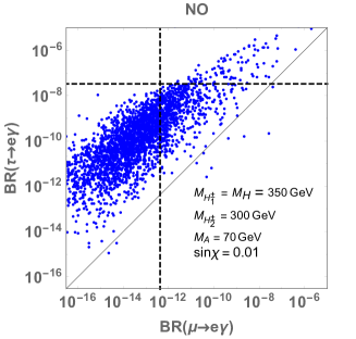
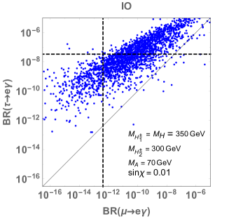
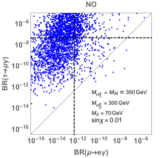
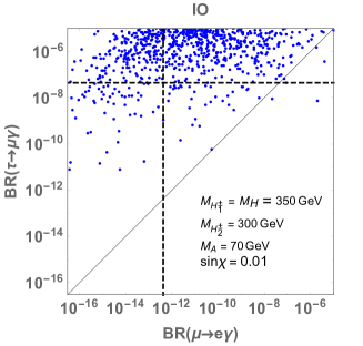
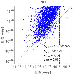
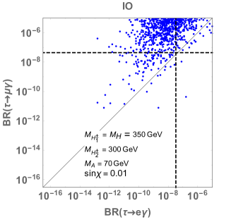
Figure 1: Correlations among BR$(\ell_{i}\to\ell_{j}\gamma)$ for the case with $m_{H_{1}^{\pm}}=m_{H}=350$ GeV, $m_{H_{2}^{\pm}}=300$ GeV, $m_{A}=70$ GeV where left(right) plots correspond to NO(IO). The dashed horizontal and vertical lines indicate the upper bounds for each BR with 90% confidence level.

In the following, we perform numerical evaluations of the neutrino mass matrix and the BRs of the CLFV decays. First, we scan the input parameters as

$$-\pi\leq\{\alpha_{AB},\delta_{\rm CPV}\}\leq\pi,\quad 1\leq\tan\beta\leq 10,\quad 10^{-5}\leq m_{0}\leq 0.1~{}\text{eV}.$$ (69)

We fix the mass parameters to be $(m_{T},m_{H},m_{H^{\pm}_{1}},m_{H_{2}^{\pm}},m_{A})=(1000,350,350,300,70)$ GeV, where the scalar boson masses are chosen such that the FOPT can be realized as we see in the next section. In addition, the other parameters are fixed to be $s_{\chi}=0.01$, $\epsilon=10^{-4}$ and $\varphi_{1,2}=\varphi_{AB}=0$. We then solve Eq. (55) to obtain $F^{AB}$ for each set of the input parameters, where we use the best fit values of the neutrino parameters $\theta_{ij}$, $|\Delta m_{\rm atom}^{2}|$ and $\Delta m_{\rm sol}^{2}$ from the global fit results Esteban et al. (2020); NuFIT 5.0 (2020) for both the NO and IO cases. Finally, we apply the alignment limit $s_{\beta-\alpha}=1$, which is supported by the current LHC data Aad et al. (2020); Sirunyan et al. (2019), and is favored by the constraint from the electroweak $\rho$ parameter in the case of $m_{H}=m_{H_{1}^{\pm}}$ .

In Fig. 1, we show the correlations between the BRs of $\ell_{i}\to\ell_{j}\gamma$ processes, where the left and right plots correspond to the NO and IO cases. The upper bounds of the BRs are indicated by the dashed lines. We find a strong prediction of $\text{BR}(\tau\to\mu\gamma)\gtrsim\text{BR}(\tau\to e\gamma)\gtrsim\text{BR}(\mu\to e\gamma)$ in both the NO and IO cases. We see that larger BRs tend to be predicted in the IO case as compared with the NO case, and only little parameter sets are allowed in the IO case. We note that if we adopt smaller $s_{\chi}$ such as $10^{-3}$, most of the parameter sets are excluded since the magnitude of $F^{AB}$ increases by one order resulting in larger BRs.

In Fig. 2, we also show correlation between BR$(\mu\to e\gamma)$ and BR$(\mu\to e)_{Al}$ where the latter is $\mu$-e conversion rate for ${}^{27}_{13}$Al. We find that $BR(\mu\to e)_{Al}>$ BR$(\mu\to e\gamma)$ in some region. These region correspond to the case where $(Y_{\Phi^{\prime}})_{11}\ll(Y_{\Phi^{\prime}})_{12(21)}$ so that $\mu\to e\gamma$ is more suppressed than $\mu$-$e$ conversion.

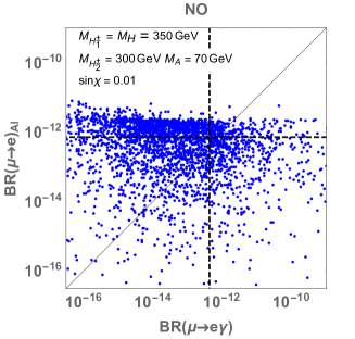
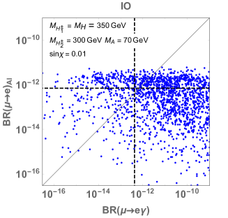
Figure 2: Correlations between BR$(\mu\to e\gamma)$ and BR$(\mu\to e)_{Al}$ for the case same as Fig. 1 where left(right) plots correspond to NO(IO). The dashed horizontal and vertical lines indicate the upper bounds for each BR with 90% confidence level.

Before closing this section, let us briefly comment on the other observables in the lepton sector under the constraints from the CLFV data. In particular, we consider the effective Majorana mass $\langle m_{ee}\rangle$ for the neutrinoless double beta decay $0\nu\beta\beta$, which can be non-zero as follows:

$$\langle m_{ee}\rangle=|m_{1}\cos^{2}{\theta_{12}}\cos^{2}{\theta_{13}}+m_{2}\sin^{2}{\theta_{12}}\cos^{2}{\theta_{13}}e^{i\varphi_{1}}+m_{3}\sin^{2}{\theta_{13}}e^{i(\varphi_{2}-2\delta_{\rm CPV})}|.$$ (70)

In our model, however, there is no particular prediction of the neutrino mixing angles, the squared mass differences and $\delta_{\rm CPV}$, so that $\langle m_{ee}\rangle$ can be obtained just by inputting the neutrino parameters which are suggested by global fit results. For example, taking the central values of the neutrino parameters and Eq. (69), we obtain $\langle m_{ee}\rangle<0.05\,(0.07)$ eV and $\sum m_{\nu}\in[0.06,0.18]\,([0.09,0.20])$ eV for the NO (IO) case. This is allowed by the current bound from the KamLAND-Zen Gando et al. (2016) experiment $\langle m_{ee}\rangle<\mathcal{O}(0.1)$ eV, while some points give the value of $\sum m_{\nu}$ larger than cosmological limit by PLANCK $\sum m_{i}<0.12$ eV Aghanim et al. (2020). In future searches for the neutrinoless double beta decay, $\langle m_{ee}\rangle$ would be probed below about 0.05 eV Gando et al. (2016), and our model can be indirectly tested.

V Collider Phenomenology of the Higgs Bosons

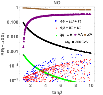
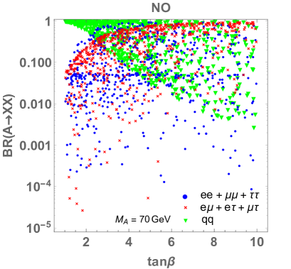
Figure 3: BRs of $H$(left) and $A$(right) for the lepton flavor conserving modes ($ee+\mu\mu+\tau\tau$), the LFV modes ($e\mu+e\tau+\mu\tau$), the hadronic modes $(\sum_{q\neq t}q\bar{q})$ modes, the $t\bar{t}$ mode and the $AA/ZA$ mode (only for $H$) as a function of $\tan\beta$; here $\ell\ell^{\prime}$ indicate the sum of $\ell^{+}\ell^{\prime-}$ and $\ell^{-}\ell^{\prime+}$ modes. The masses of $H$ and $A$ are fixed to be 350 GeV and 70 GeV, respectively.

In this section, we discuss the collider phenomenology of our model, especially focusing on the lepton flavor violating (LFV) decays of the additional neutral Higgs bosons $H$ and $A$. Such LFV decays are induced from the Yukawa matrices $Y_{\Phi}$ and $Y_{\Phi^{\prime}}$, whose values are constrained by the charged lepton masses, neutrino oscillation data and the CLFV data, so that we expect the appearance of a characteristic pattern of the decay BRs. We here consider only the NO case adopting parameter sets satisfying CLFV constraints in previous section; IO case gives similar behavior of neutral scalar boson decay BRs.

As in the previous section, we scan the parameters written in Eq. (69), and take $s_{\beta-\alpha}=1$, $s_{\chi}=0.01$, $\epsilon=10^{-4}$ and the masses $(m_{T},m_{H},m_{H_{1}^{\pm}},m_{H_{2}^{\pm}},m_{A})=(1000,350,350,300,70)$ GeV. Due to the choice of the mass spectrum, the $H\to ZA$ and $H\to AA$ decays can be important whose decay rates are calculated as

$$\Gamma(H\to ZA) =\frac{g^{2}}{64\pi\cos^{2}{\theta_{W}}}\frac{m_{H}^{3}}{m_{Z}^{2}}\left[\left(1-\frac{m_{Z}^{2}}{m_{H}^{2}}-\frac{m_{A}^{2}}{m_{H}^{2}}\right)^{2}-\frac{4m_{Z}^{2}m_{A}^{2}}{m_{H}^{4}}\right]^{3/2},$$ (71)

$$\Gamma(H\to AA) =\frac{\lambda_{HAA}^{2}}{8\pi m_{H}}\sqrt{1-\frac{4m_{A}^{2}}{m_{H}^{2}}},$$ (72)

where $\theta_{W}$ is the Weinberg angle and $\lambda_{HAA}=(m_{H}^{2}-m_{A}^{2})\cot 2\beta/v$. Differently from the leptonic decays of the Higgs bosons, decay rates into a quark pair are the same as those given in the Type-I THDM. Thus, among the hadronic decays, the decay rates of $H/A\to b\bar{b}$ $(H/A\to t\bar{t})$ can be dominant for the Higgs boson mass below (above) twice of the top quark mass. We note that the decay modes of $H\to ZZ/W^{+}W^{-}/hh$ and $A\to Zh$ are absent in the alignment limit at tree level.

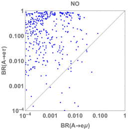
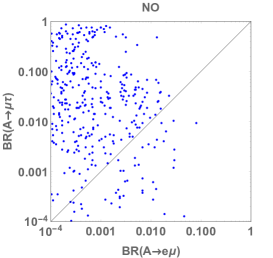
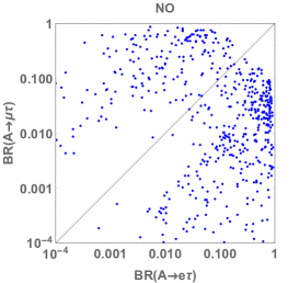
Figure 4: Correlations among ${\rm BR}(A\to\ell_{i}\ell_{j})$ shown where the mass of $A$ is fixed to be 70 GeV.

In Fig. 3, we show the BRs of $H$ and $A$ for the sum of the lepton flavor conserving modes, that of the LFV modes ($\ell_{i}\ell_{j}$ indicate the sum of $\ell^{+}_{i}\ell^{-}_{j}$ and $\ell^{+}_{j}\ell^{-}_{i}$), that of the hadronic modes (only the $t\bar{t}$ mode is separately shown) and the $AA/ZA$ modes (only for $H$) as a function of $\tan\beta$, fixing the masses to be $m_{H}=350$ GeV and $m_{A}=70$ GeV. The dominant mode of the $H$ decay is the $ZA$ mode, and the $AA$ or $t\bar{t}$ mode is the second largest one depending on $\tan\beta$, while the leptonic decay modes are smaller than $10^{-3}$. The $H\to AA$ mode becomes significant for larger values of $\tan\beta$, because of the enhancement of the coupling $\lambda_{HAA}\sim-(m_{H}^{2}-m_{A}^{2})\tan\beta/(2v)$ for $\tan\beta\gg 1$. For the $A$ decay, the LFV modes can be dominant for $\tan\beta\gtrsim 3$, since Higgs to Higgs decays and the $t\bar{t}$ mode are kinematically forbidden. The correlations of the LFV decay modes of $A$ can be seen in Fig. 4. We find that BR$(A\to e\mu)$ tends to be smaller than the other LFV decay modes, while both BR$(A\to e\tau)>$BR$(A\to\mu\tau)$ and BR$(A\to e\tau)<$BR$(A\to\mu\tau)$ cases can be found with similar amount.

We here comment on the decay of the SM-like Higgs boson $h$. In the THDMs, the couplings of $h$ coincide with those of the SM Higgs boson in the alignment limit at tree level. In our model, however, the Yukawa matrix $Y_{\Phi}$ is not exactly the same as the SM one even in the alignment limit, i.e., non-zero off-diagonal elements appear in the fermion mass eigenbasis. Such off-diagonal component is highly suppressed by the factor of $\epsilon^{2}$, so that the size of BRs of LFV decays of $h$ can be estimated by ${\cal O}(\epsilon^{4})$. In fact, we numerically checked that the magnitude of BR$(h\to\ell\ell^{\prime})$ is quite small, ${\cal O}(10^{-16})$ or less, in our benchmark scenario with $\epsilon=10^{-4}$. This should be compared with the property of the additional Higgs bosons, in which the second Yukawa matrix $Y_{\Phi^{\prime}}$ determines the decays of these Higgs bosons, and its off-diagonal elements are not suppressed by the $\epsilon$ factor, see Eq. (21).

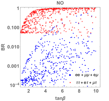
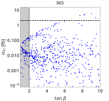
Figure 5: (Left) Sum of the BRs of $A$ into $ee$, $e\mu$ and $\mu\mu$ (blue points) and that into $e\tau$, $\mu\tau$ and $\tau\tau$ (red points) as a function of $\tan\beta$ for $m_{A}=70$ GeV. (Right) Cross section of the four lepton ($e$ or $\mu$) final states $\sigma_{4\ell}$ calculated by using Eq. (73) with $\ell=e$ or $\mu$ as a function of $\tan\beta$ for $m_{A}=70$ GeV and $m_{H}=350$ GeV. The dashed line indicates the current upper limit on the cross section given by the LHC data Khachatryan et al. (2017). The shaded region is excluded by the constraint from $B_{d}\to\mu\mu$ Arbey et al. (2018); Haller et al. (2018).

Let us move on to the discussion of production processes of the additional Higgs bosons and constraints from current LHC data. At the LHC, the additional Higgs bosons can mainly be produced via the gluon fusion process $gg\to H/A$. The pair productions $pp\to HA/H^{\pm}H/H^{\pm}A$ can also be used for smaller mass cases. So far, no discovery of significant signatures has been reported, and it has taken lower limits on their masses and upper limits on relevant coupling constants. See, e.g., Ref. Aiko et al. (2020) for the recent analysis of the constraints from direct searches at the LHC in the THDM. We see in Aiko et al. (2020) that in the alignment limit $s_{\beta-\alpha}=1$ with degenerate masses of the additional Higgs bosons, most of the parameter region has not been excluded yet, e.g., $\tan\beta\gtrsim 2$ is allowed in the Type-I THDM. It is important to mention here that these searches typically have sensitivities to relatively larger mass regions, e.g., above 100 GeV, so that they cannot be simply applied to cases for lighter additional Higgs bosons and/or the case with mass differences.

From the above analysis, we see that $H$ can mainly decay into $ZA$ and $AA$, and $A$ further decays into a lepton pair. Thus, clear signals of $H$ can be obtained by the decay chain of $H\to ZA/AA\to 4\ell$, and its cross section can be estimated by

$$\sigma_{4\ell} \simeq\sigma(gg\to H)\times[\text{BR}(H\to ZA)\times\text{BR}(A\to\ell\ell)\times\text{BR}(Z\to\ell\ell)$$

$$+\text{BR}(H\to AA)\times\text{BR}(A\to\ell\ell)^{2}],$$ (73)

where $\sigma(gg\to H)$ is the gluon fusion cross section for $H$, which can be estimated to be $4~{}{\rm pb}\times\cot^{2}\beta$ for $m_{H}=350$ GeV de Florian et al. (2016). A similar process with the same final states has been searched at the LHC, i.e., $pp\to Z^{\prime}\to\phi\phi(\phi\to 2\ell)$ process ($\ell=e,\mu$) with $Z^{\prime}$ and $\phi$ being an extra neutral gauge boson and a neutral scalar boson, respectively. For $m_{Z^{\prime}}=350$ GeV which can be replaced by $m_{H}$ in our case, the upper limit has been set to be $\sigma_{4\ell}\sim 2$ fb Khachatryan et al. (2017). In the left panel of Fig. 5, we show the sum of the BRs of $A\to\ell\ell$ ($\ell=e$ or $\mu$) and that including at least one $\tau$. We see that the former quantity rapidly increases as $10^{-3}$, $10^{-2}$ and $10^{-1}$ at $\tan\beta\simeq 2$, 4 and 6, respectively, so that at high $\tan\beta$ some parameter points can be excluded by the current LHC data. In fact, as seen in the right panel of Fig. 5, a portion of points exceeds the current upper limit of $\sigma_{4\ell}$ at around $\tan\beta\simeq 8$, while the case with even larger $\tan\beta$ is not excluded because the cross section is suppressed by $\cot^{2}\beta$ and the maximal value of the BR is saturated. In addition excluded cases correspond to $(Y_{\Phi^{\prime}})_{ij}\ (i[j]=1,2)\gtrsim(Y_{\Phi^{\prime}})_{3a(a3)}\ (a=1,2,3)$ in which the BR of modes including $\tau$ are smaller than the modes including only $e$ and/or $\mu$. Therefore, our model is allowed by the current LHC data except for quite a few cases, and could be test at future collider experiments. Moreover, LFV decay signals with $\tau$ would significantly improve the testability of the model, since the cross section $\sigma_{4\ell}$ including $\tau$ is much larger than the signals including only $e$ and/or $\mu$.

Finally, let us give a comment on the phenomenology of the light CP-odd Higgs boson. For $m_{A}<m_{h}/2$, $h\to AA$ is allowed, and bounds on such BRs of the Higgs to Higgs decays have been studied in Ref. Bernon et al. (2015) in the THDM. In our scenario with $m_{A}=70$ GeV, these decays are kinematically forbidden. In the intermediate mass range, i.e., $62.5\lesssim m_{A}\lesssim 100$ GeV, the search for additional Higgs bosons decaying into diphoton is available CMS (2017) at the LHC, where the value of cross section times BR has been constrained to be smaller than about 0.1 pb with the 95% confidence level. In our model, the gluon fusion production of $A$ with the mass of 70 GeV is given to be about 40 pb$\times\cot^{2}\beta$ de Florian et al. (2016), while the BR of $A\to\gamma\gamma$ is given of order $10^{-4}$. Therefore, the cross section times BR is much below the current upper limit. At future collider experiments such as the High-Luminosity LHC CMS (2013); ATL (2013) and lepton colliders, e.g., the International Linear Collider (ILC) Baer et al. (2013); Asai et al. (2017); Fujii et al. (2019), the Circular Electron-Positron Collider (CEPC) Group (2015) and the Future Circular Collider (FCC-ee) Bicer et al. (2014), our scenario could be tested via the LFV decays of the Higgs bosons with the characteristic decay pattern. It goes without saying that dedicated studies are required to clarify the feasibility of such signatures, and such analyses are beyond the scope of the present paper.

VI Electroweak Phase Transition

In this section, we consider the cosmological consequences of our scenario, particularly focusing on the electroweak phase transition. It has been known that in the electroweak baryogenesis scenario Kuzmin et al. (1985); Shaposhnikov (1987), the strongly FOPT is required to realize sufficient departure from thermal equilibrium in order to maintain non-zero baryon asymmetry of the Universe. The criteria for the strongly FOPT can be expressed by $\varphi_{c}/T_{c}\gtrsim 1$ or $\varphi_{n}/T_{n}\gtrsim 1$, where $T_{c}$ $(T_{n})$ is the critical temperature providing degenerate vacua (nucleation temperature of electroweak bubbles from the bounce solution) and $\varphi_{c}$ $(\varphi_{n})$ is the order parameter at $T_{c}\,(T_{n})$. Although we should use $\varphi_{n}/T_{n}$ rather than $\varphi_{c}/T_{c}$ for the estimation of the strength of the FOPT, we show both of them for comparison. Typically, these two valuables are almost the same with each other unless considering a mechanism of the supercooling scenario in which the thermal barrier does not disappear until much lower temperature $T_{n}\ll T_{c}$ Iso et al. (2017); von Harling and Servant (2018).

It has been known that additional bosons can enhance the FOPT Dolan and Jackiw (1974), because their loop effects provide a positive contribution to a cubic field term of the effective potential at finite temperature, which makes a potential barrier higher at around the critical temperature. Indeed, it has been clarified that additional Higgs bosons in the THDM can make the FOPT stronger as a consequence of the non-decoupling effect if their masses mainly come from the VEV Kanemura et al. (2005). This can also be described in such a way that a new dimensionful parameter $M$ which is irrelevant to the VEV and appears in the mass of Higgs bosons is taken to be smaller than the physical mass parameter of the additional Higgs bosons. In our model, such $M$ parameter directly corresponds to the mass of $A$, see Eq. (27), so that $m_{A}$ has to be smaller than the other masses of the additional Higgs bosons in order to enhance the FOPT. In Appendix C, we present detailed analytic expressions for the effective potential at finite temperature. We note that the loop effect of the charged singlet fields $S^{\pm}$ can not be dominant in our model, because of the smaller degrees of freedom $(N=2)$ as compared with those of the doublets $(N=8)$. We numerically find that the FOPT can be maximal when the mass of singlet-like Higgs boson $m_{H_{2}^{\pm}}$ is taken to be around 300 GeV in our scenario.

In the following, we numerically evaluate the strength of the FOPT, i.e., $\varphi_{c}/T_{c}$ or $\varphi_{n}/T_{n}$ by using CosmoTransitions Wainwright (2012). We have checked that the behavior of the FOPT in the case of the THDM is consistent with the previous work Basler et al. (2017). Our model predictions can then be simply obtained by taking $M=m_{A}$ in the THDM and modifying the charged Higgs sector by that with $H_{1}^{\pm}$ and $H_{2}^{\pm}$. As mentioned above, we take a smaller value of $m_{A}$ but larger than $m_{h}/2$, e.g., 70 GeV, to avoid the constraint from $h\to AA$ at the LHC, see previous section. In addition, we take into account the constraints from perturbative unitarity and vacuum stability discussed in Sec. II and flavor experiments Arbey et al. (2018); Haller et al. (2018) such as $B_{d}\to\mu\mu$.

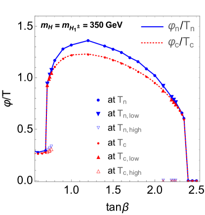
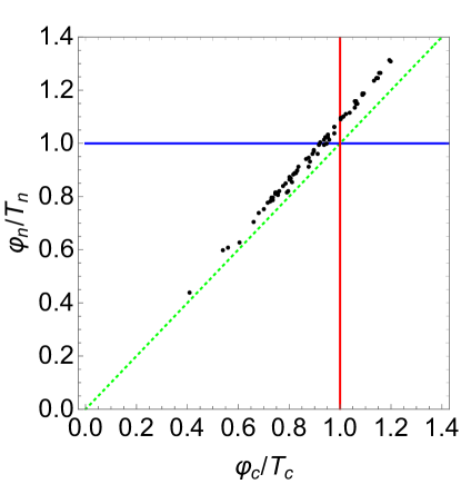
Figure 6: (Left) Strength of the FOPT $\varphi/T$ at the critical temperature $T_{c}$ (red) and the bubble nucleation temperature $T_{n}$ (blue) as a function of $\tan\beta$ in the case of $(m_{A},m_{H},m_{H_{1}^{\pm}},m_{H_{2}^{\pm}})=(70,350,350,300)$ GeV, $m_{S}=0$, $s_{\chi}=0$, $\tan\sigma=1$ and $s_{\beta-\alpha}=1$. At the circle (triangle) points, the one-step (two-step) phase transition is realized, in which the empty (filled) triangles show the temperature at the first (second) phase transition denoted by $T_{c(n),\text{high}}$ ($T_{c(n),\text{low}}$) with $T_{c(n),\text{high}}>T_{c(n),\text{low}}$. Points at $\varphi/T=0$ indicate the second-order phase transition. (Right) Correlation between $\varphi_{c}/T_{c}$ and $\varphi_{n}/T_{n}$ with the scan of $m_{H}$ $(=m_{H_{1}^{\pm}})$ $\in$ [180, 500] GeV and $\tan\beta\in[1.4,3.0]$. All the other parameters are taken in the same way as those of the left plot.

In Fig. 6 (left), we show $\varphi_{c}/T_{c}$ and $\varphi_{n}/T_{n}$ as a function of $\tan\beta$ for the case with $m_{A}=70$ GeV, $m_{H}=m_{H_{1}^{\pm}}=350$ GeV and $m_{H_{2}^{\pm}}=300$ GeV. We here neglect the effect of the small mixing angle between two charged Higgs bosons. For concreteness, we take $s_{\chi}=0$. In this plot, we do not impose the constraints from the flavor experiments and the unitarity bound. We find that in some parameter points indicated by the triangle a two-step phase transition happens, where the empty (filled) triangles represent the value of $\varphi_{c}/T_{c}$ or $\varphi_{n}/T_{n}$ at the first (second) transition, while the circle points represent the case with the one-step phase transition. We see that both $\varphi_{c}/T_{c}$ or $\varphi_{n}/T_{n}$ become maximal at around $\tan\beta=1.2$, and $\varphi_{c}/T_{c}$ $(\varphi_{n}/T_{n})$ is greater than unity at $0.7\lesssim\tan\beta\lesssim 1.9$ ($0.7\lesssim\tan\beta\lesssim 2.0$). In addition, the value of $\varphi_{n}/T_{n}$ is slightly larger than $\varphi_{c}/T_{c}$, which can be more clearly seen from the right panel of Fig. 6, in which we show the correlation between $\varphi_{c}/T_{c}$ and $\varphi_{n}/T_{n}$. We see that $\varphi_{n}/T_{n}$ is typically about 10% larger than $\varphi_{c}/T_{c}$. This can mainly be explained by the difference between $\varphi_{c}$ and $\varphi_{n}$ ($\varphi_{n}>\varphi_{c}$) whose values are quite sensitive to the temperature at around the phase transition. In fact, around the $10\%$ difference between $\varphi_{c}$ and $\varphi_{n}$ arises from the slight difference between the temperatures, i.e., $(T_{c}-T_{n})/T_{c}=\mathcal{O}(10^{-3})$.

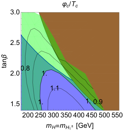
Figure 7: Contour plots of $\varphi/T$ at $T_{c}$ (left) and $T_{n}$ (right) in the $m_{H}(=m_{H_{1}^{\pm}})$-$\tan\beta$ plane, respectively. We take a parameter set used in the right panel of Fig. 6. The green shaded region does not satisfy the criteria for the FOPT, i.e., $\varphi/T\gtrsim 1$. The blue and brown shaded region are respectively excluded by the constraint from $B_{d}\to\mu\mu$ Arbey et al. (2018); Haller et al. (2018) and the unitarity bound given in Eq. (40).

In Fig. 7, we show the contour plots for $\varphi/T$ at $T=T_{c}$ (left) and $T=T_{n}$ (right) in the $m_{H}(=m_{H_{1}^{\pm}})$-$\tan\beta$ plane using the same parameter set taken in the right panel of Fig. 6. Under the constraints from the flavor experiments and the unitarity bound, we find that there is a region of the parameter space which realizes the strongly FOPT ($\varphi_{n}/T_{n}\gtrsim 1$) shown as the white area in the right panel. It is clear that such region requires the quite limited parameter choice, i.e., $1.9\lesssim\tan\beta\lesssim 2.3$ and $250\lesssim m_{H}\lesssim 400$ GeV, which provides a good benchmark scenario for the collider phenomenology, as we discussed it in the previous section.

It is worth discussing detectability of the gravitational waves (GWs) originated from the first-order phase transition since the typical frequency of GWs from the first-order phase transition at the electroweak scale is expected to explore by future planned space-based interferometers such as LISA Seoane et al. (2013), DECIGO Kawamura et al. (2011) and BBO Corbin and Cornish (2006) which survey GWs in the millihertz to decihertz range. The GW spectrum can be parameterized by two dimensionless parameters, related to the released energy density $\epsilon$ and the change rate of the three dimensional bounce action $S_{3}$, defined as

$$\alpha\equiv\left.\frac{\epsilon}{\rho_{\text{rad}}}\right|_{T=T_{n}},\quad\widetilde{\beta}\equiv\left.\frac{d(S_{3}/T)}{d\ln T}\right|_{T=T_{n}},$$ (74)

where $\rho_{\text{rad}}$ is the radiation energy density. We employ the analytic formula provided in Ref. Caprini et al. (2016) to estimate the spectrum of the GWs, $\Omega_{\text{GW}}h^{2}(f)$. Parameters have one-to-one correspondence $(\tan\beta,m_{H})\leftrightarrow(\alpha,\widetilde{\beta})\leftrightarrow(f,\Omega_{\text{GW}}h^{2})$ and correlations with the phase transition strength $\varphi_{n}/T_{n}\propto\Omega_{\text{GW}}h^{2}\propto\alpha\propto\widetilde{\beta}^{-1}$.

In Fig. 8, the predicted GW signals are plotted taking parameters on Fig. 7. Red colors on each panel are allowed by the constraint from $B_{d}\to\mu\mu$. We find that the GW signals do not reach the future planned sensitivities of observations. Because the exact non-decoupling limit does not allow due to the global U(1) and the constraint from $B_{d}\to\mu\mu$ excluds most of the parameter space, the GW signals correlated with the strength of the first-order phase transition cannot be enough strong.

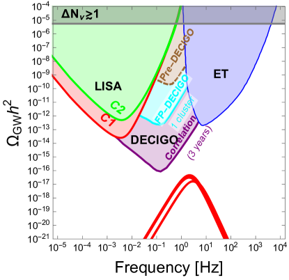
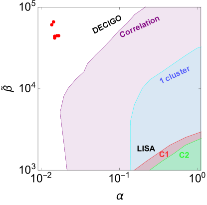
Figure 8: (Left) Predicted GW signals originated from the first-order phase transition are plotted with red lines, taking parameters on Fig. 7. The analytic formula provided in Ref. Caprini et al. (2016) is used to estimate the spectrum of the GWs assuming the bubble wall velocity $v_{b}$ = 0.95 as an example. Sensitivity curves for future GW interferometers, LISA Caprini et al. (2016), DECIGO Kawamura et al. (2011), and Einstein telescope (ET) Schmitz (2020) are plotted, respectively. (Right) Predicted values of $\alpha$ and $\widetilde{\beta}$ which derive the plot on the left panel. Experimental sensitivities are obtained for the sound wave contribution fixing $T_{n}$ = 100 GeV.

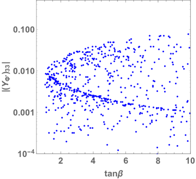
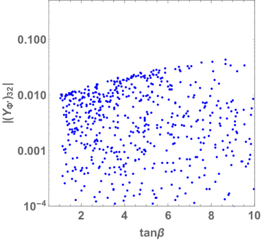
Figure 9: Values of $(Y_{\Phi^{\prime}})_{33}$ (left) and $(Y_{\Phi^{\prime}})_{32}$ (right) couplings as a function of $\tan\beta$.

Finally, we give a comment on the possibility for the generation of baryon asymmetry of the Universe. As it is known that the strongly FOPT is one of the necessary conditions to obtain the non-zero baryon number in the electroweak phase transition. In order to estimate the generated baryon number, we also need to calculate the reflection rate of chiral fermions against the bubble, in which non-zero charges, e.g., the hypercharge and isospin, can be accumulated at the vicinity of the bubble if CP-violation happens in the interaction among the bubble and fermions. Such non-zero charges can be converted into the baryon number from the sphaleron process, which is frozen in the broken phase because of the decoupling of the sphaleron process. See e.g., Funakubo (1996) for more detailed discussions. In Ref. Chiang et al. (2016), the electroweak baryogenesis has been discussed in a two Higgs doublet model by introducing CP-violating phases in lepton Yukawa couplings, particularly $\tau$-$\tau$ and $\tau$-$\mu$ couplings to additional Higgs bosons. It has been shown that in order to explain the observed baryon asymmetry the magnitude of these Yukawa couplings has to be of order 0.1–1. We thus plot the values of corresponding Yukawa couplings $(Y_{\Phi^{\prime}})_{33}$ and $(Y_{\Phi^{\prime}})_{32}$ in our model in Fig. 9. It is seen that in the region where the FOPT is realized, i.e., $\tan\beta\simeq 2$, the value of $(Y_{\Phi^{\prime}})_{33}$ and $(Y_{\Phi^{\prime}})_{32}$ can be maximally of order 0.01. Therefore, qualitatively our model can generate baryon asymmetry which is one or two orders of magnitude smaller than the required value, so that additional sources of baryon asymmetry would be needed.

VII Conclusions

We have investigated the Zee model which is extended by introducing a vector-like lepton doublet and a flavor dependent global $U(1)^{\prime}$ symmetry. Because of the $U(1)^{\prime}$ symmetry, FCNCs in the quark sector can naturally be avoided at tree level, while a sufficient new source of LFV interactions is provided, which is required to explain the current neutrino oscillation data. In particular, we have focused on the weak mixing scenario, where the fourth charged lepton is weakly mixed, with a magnitude of $\epsilon(\ll 1)$, with three generations of the SM leptons. This scenario can successfully suppress CLFV decays, but give an important new contribution to the neutrino mass matrix. By scanning model parameters under which neutrino oscillation data are satisfied, we have shown the appearance of strong correlations among the BRs of CLFV decays, i.e., $\text{BR}(\tau\to\mu\gamma)\gtrsim\text{BR}(\tau\to e\gamma)\gtrsim\text{BR}(\mu\to e\gamma)$ in both the NO and IO cases.

Our model provides additional sources of CP-violation in the lepton sector. We thus have studied an impact of these CP-violating phases on the electron EDM. It is shown that the new contribution to the electron EDM is sufficiently smaller than the current experimental limit, because of the structure of the Yukawa matrices constrained by the $U(1)^{\prime}$ symmetry and the weak mixing scenario. Thus, our scenario is allowed even if we take ${\cal O}(1)$ phases of the lepton sector.

We then have discussed the collider phenomenology, especially focusing on the LFV decays of the neutral Higgs bosons. In our benchmark scenario motivated by realization of the strongly FOPT, the additional CP-even Higgs boson $H$ mainly decays into the light CP-odd Higgs boson $A$ such as $ZA$ or $AA$, and $A$ dominantly decays into a lepton pair with both lepton flavor conserved and violated one. Thus, the four lepton final states are expected at the LHC via $pp\to H\to ZA/AA\to\ell_{i}\ell_{j}\ell_{k}\ell_{l}$. We have confirmed that the cross section of this process is below the current upper limit driven by the LHC data, except for a small portion of the parameters allowed by the CLFV data with $\tan\beta\simeq 8$. This signature can be a smoking gun to probe our model, and would be tested at future collider experiments such as the HL-LHC and future lepton colliders.

Finally, as a cosmological consequence, we have studied the electroweak phase transition by using the effective potential at finite temperature. The content of the Higgs sector in our model is the same as that of the original Zee model, i.e., two Higgs doublets and a pair of charged singlet scalars. Due to the $U(1)^{\prime}$ symmetry, the coefficient of the $(\Phi_{1}^{\dagger}\Phi_{2})^{2}$, denoted as $\lambda_{5}$, is forbidden, and thus the CP-odd Higgs boson $A$ becomes a pseudo-NG boson whose mass arises from the $(\Phi_{1}^{\dagger}\Phi_{2})$ term. Because of this property, we need a light $A$ in order to make non-decoupling effects of the additional Higgs bosons stronger, which plays an important role to realize the strongly FOPT. We have found that the strongly FOPT can be realized in the case where $1.9\lesssim\tan\beta\lesssim 2.3$ and $250\lesssim m_{H}\lesssim 400$ GeV for $m_{A}=70$ GeV, which is compatible with the constraints from the flavor experiments and LHC data. Therefore, we have shown that our model contains two important ingredients to realize the successful electroweak baryogenesis scenario, i.e., the additional CP-violating phases and the strongly FOPT. According to the qualitative discussion, our model can generate baryon asymmetry which is one or two orders of magnitude smaller than its observed amount, so that additional sources of baryon asymmetry would be required.

Appendix A Approximate Formulae for the $F$ Matrix

In Sec. III, we show that the matrix elements $F$ can be expressed in terms of the neutrino mass matrix by solving Eq. (55). Neglecting the electron mass except for terms proportional to $1/m_{e}$, we find the following approximate formulae for the elements of the $F$ matrix:

$$\begin{split}F_{12}&\simeq\frac{m_{\rm dat}^{11}}{2C_{\rm diag}^{0}m_{\mu}}\frac{\delta_{24}y_{33}-y_{23}\delta_{34}}{y_{12}\delta_{24}y_{33}+\delta_{14}y_{23}y_{32}+y_{13}y_{22}\delta_{34}-y_{12}y_{23}\delta_{34}-y_{13}\delta_{24}y_{32}-\delta_{14}y_{22}y_{33}},\\ F_{13}&\simeq-\frac{m_{\rm dat}^{11}}{2C_{\rm diag}^{0}m_{\tau}}\frac{\delta_{24}y_{32}-\delta_{34}y_{22}}{y_{12}\delta_{24}y_{33}-y_{12}y_{23}\delta_{34}+y_{13}y_{22}\delta_{34}-y_{13}\delta_{24}y_{32}-\delta_{14}y_{22}y_{33}+\delta_{14}y_{23}y_{32}},\\ F_{23}&\simeq-\frac{m_{\rm dat}^{33}\delta_{24}^{2}-2m_{\rm dat}^{23}\delta_{24}\delta_{34}+m_{\rm dat}^{22}\delta_{34}^{2}}{2C_{\rm diag}^{0}\left[m_{\mu}\delta_{24}(\delta_{24}y_{32}-y_{22}\delta_{34})+m_{\tau}\delta_{34}(\delta_{24}y_{33}-y_{23}\delta_{34})\right]},\\ F_{14}&\simeq\frac{m_{\rm dat}^{11}}{2C_{\rm diag}^{4}m_{T}}\frac{y_{23}y_{32}-y_{22}y_{33}}{y_{12}\delta_{24}y_{33}+\delta_{14}y_{23}y_{32}+y_{13}y_{22}\delta_{34}-y_{12}y_{23}\delta_{34}-y_{13}\delta_{24}y_{32}-\delta_{14}y_{22}y_{33}},\\ F_{24}&\simeq\frac{m_{\rm dat}^{22}(\delta_{24}y_{32}r-y_{22}\delta_{34}r+\delta_{34}y_{33})+y_{23}\delta_{24}m_{\rm dat}^{33}-2m_{\rm dat}^{23}y_{23}\delta_{34}}{2C_{\rm diag}^{4}m_{T}\left[(r\delta_{24}(\delta_{24}y_{32}-\delta_{34}y_{22})+\delta_{34}(\delta_{24}y_{33}-y_{23}\delta_{34})\right]},\\ F_{34}&\simeq\frac{m_{\rm dat}^{33}(\delta_{24}y_{33}-y_{23}\delta_{34}-ry_{22}\delta_{24})+2rm_{\rm dat}^{23}\delta_{24}y_{32}-rm_{\rm dat}^{22}y_{32}\delta_{34}}{2C_{\rm diag}^{4}m_{T}\left[r\delta_{24}(\delta_{24}y_{32}-y_{22}\delta_{34})+\delta_{34}(\delta_{24}y_{33}-\delta_{34}y_{23})\right]},\end{split}$$ (75)

where $y_{ij}\equiv(Y_{\Phi^{\prime}}^{0})_{ij}$, $\delta_{ij}\equiv(\delta Y_{\Phi^{\prime}})_{ij}$ and $r\equiv m_{\mu}/m_{\tau}$. The matrix elements $m_{\rm dat}^{ij}$ denote those of the right-hand side of Eq. (53). These expressions agree with the exact ones typically within a 10% error.

Appendix B Decay Amplitudes for $\ell_{i}\to\ell_{j}\gamma$ Processes

Here, we summarize the analytic formulae for the amplitudes of the $\ell_{i}\to\ell_{j}\gamma$ processes denoted by $(a_{L,R})_{ij}$ in Eq. (65). The contributions from diagrams with the charged Higgs bosons inside loop are obtained as

$$(a_{R}^{H^{\pm}_{1}})_{ij} =\frac{1}{16\pi^{2}}\sum_{A=1}^{4}\left[(Y_{\Phi^{\prime}})_{Aj}^{*}(Y_{\Phi^{\prime}})_{Ai}c_{\chi}^{2}F_{1}(m_{\ell_{i}},m_{\ell_{j}},m_{H_{1}^{\pm}})-F_{Aj}^{*}F_{Ai}s_{\chi}^{2}F_{2}(m_{\ell_{i}},m_{\ell_{j}},m_{H_{2}^{\pm}})\right],$$ (76)

$$(a_{L}^{H^{\pm}_{1}})_{ij} =\frac{1}{16\pi^{2}}\sum_{A=1}^{4}\left[(Y_{\Phi^{\prime}})_{Aj}^{*}(Y_{\Phi^{\prime}})_{Ai}c_{\chi}^{2}F_{2}(m_{\ell_{i}},m_{\ell_{j}},m_{H_{1}^{\pm}})-F_{Aj}^{*}F_{Ai}s_{\chi}^{2}F_{1}(m_{\ell_{i}},m_{\ell_{j}},m_{H_{2}^{\pm}})\right],$$ (77)

$$(a_{R}^{H^{\pm}_{2}})_{ij} =(a_{R}^{H^{\pm}_{1}})_{ij}\Big{|}_{c_{\chi}^{2}\leftrightarrow s_{\chi}^{2}},\quad(a_{L}^{H^{\pm}_{2}})_{ij}=(a_{L}^{H^{\pm}_{1}})_{ij}\Big{|}_{c_{\chi}^{2}\leftrightarrow s_{\chi}^{2}}.$$ (78)

The loop functions are defined by

$$F_{1[2]}(m_{1},m_{2},m_{3})=\int[dX]\frac{xzm_{2}[xym_{1}]}{(x^{2}-x)m_{1}^{2}+xz(m_{1}^{2}-m_{2}^{2})+(y+z)m_{3}^{2}},$$ (79)

where we write $\int[dX]\equiv\int_{0}^{1}dxdydz\delta(1-x-y-z)$. The contributions from diagrams with the neutral scalar bosons ($\varphi=h,H,A$) inside loop are calculated as

$$(a_{R}^{\varphi})_{ij}=\frac{1}{8\pi^{2}}\sum_{A=1}^{4}\int[dX]\frac{xym_{\ell_{i}}f^{*jA}_{\varphi}f^{Ai}_{\varphi}+xzm_{\ell_{j}}g^{*jA}_{\varphi}g^{Ai}_{\varphi}+(1-x)m_{\ell_{A}}f^{*jA}_{\varphi}g^{Ai}_{\varphi}}{-x(1-x)m^{2}_{\ell_{i}}-xz(m^{2}_{\ell_{j}}-m^{2}_{\ell_{i}})+(z+y)m^{2}_{\ell_{A}}+xm_{\varphi}^{2}},$$ (80)

$$(a_{L}^{\varphi})_{ij}=\frac{1}{8\pi^{2}}\sum_{A=1}^{4}\int[dX]\frac{xzm_{\ell_{i}}f^{*jA}_{\varphi}f^{Ai}_{\varphi}+xym_{\ell_{j}}g^{*jA}_{\varphi}g^{Ai}_{\varphi}+(1-x)m_{\ell_{A}}g^{*jA}_{\varphi}f^{Ai}_{\varphi}}{-x(1-x)m^{2}_{\ell_{i}}-xz(m^{2}_{\ell_{j}}-m^{2}_{\ell_{i}})+(z+y)m^{2}_{\ell_{A}}+xm_{\varphi}^{2}},$$ (81)

where the couplings corresponding to the neutral scalars $\varphi$ are given by

$$f^{AB}_{h}=\frac{1}{\sqrt{2}}(Y_{\Phi}^{*})_{BA}s_{\beta-\alpha}+\frac{1}{\sqrt{2}}(Y_{\Phi^{\prime}}^{*})_{BA}c_{\beta-\alpha},\quad g^{AB}_{h}=\frac{1}{\sqrt{2}}(Y_{\Phi})_{AB}s_{\beta-\alpha}+\frac{1}{\sqrt{2}}(Y_{\Phi^{\prime}})_{AB}c_{\beta-\alpha}$$

$$f^{AB}_{H}=\frac{1}{\sqrt{2}}(Y_{\Phi}^{*})_{BA}c_{\beta-\alpha}-\frac{1}{\sqrt{2}}(Y_{\Phi^{\prime}}^{*})_{BA}s_{\beta-\alpha},\quad g^{AB}_{H}=\frac{1}{\sqrt{2}}(Y_{\Phi})_{AB}c_{\beta-\alpha}-\frac{1}{\sqrt{2}}(Y_{\Phi^{\prime}})_{AB}s_{\beta-\alpha}$$

$$f^{AB}_{A}=-\frac{i}{\sqrt{2}}(Y_{\Phi^{\prime}}^{*})_{BA}c_{\beta-\alpha},\quad g^{AB}_{A}=\frac{i}{\sqrt{2}}(Y_{\Phi})_{AB}c_{\beta-\alpha}.$$ (82)

Appendix C One-loop Effective Potential at Finite Temperature

In order to discuss the one-loop effective potential at finite temperature, we introduce the classical constant field configurations $\vec{\varphi}=(\varphi_{1},\varphi_{2})$ where $(\varphi_{1},\varphi_{2})|_{T=0}\equiv(v_{1},v_{2})$ at the VEVs of our present vacuum. We here do not consider the possibility of CP-breaking and/or charge-breaking vacua for simplicity.

The effective potential receives additional contributions from thermal loop diagrams, and is modified to Dolan and Jackiw (1974)

$$V_{\text{eff}}(\vec{\varphi},T)=V_{\text{tree}}(\vec{\varphi})+V_{\text{CW}}[M_{i}(\vec{\varphi},T)]+V_{T}\left[M_{i}(\vec{\varphi},T)\right],$$ (83)

with

$$V_{\text{tree}}(\vec{\varphi}) \equiv\frac{m_{1}^{2}}{2}\varphi_{1}^{2}+\frac{m_{2}^{2}}{2}\varphi_{2}^{2}-m_{3}^{2}\varphi_{1}\varphi_{2}+\frac{\lambda_{1}}{8}\varphi_{1}^{4}+\frac{\lambda_{2}}{8}\varphi_{2}^{4}+\frac{1}{4}(\lambda_{3}+\lambda_{4})\varphi_{1}^{2}\varphi_{2}^{2},$$ (84)

$$V_{\text{CW}}\left[M_{i}(\vec{\varphi})\right] \equiv\sum_{i}\frac{n_{i}}{64\pi^{2}}M_{i}^{4}(\vec{\varphi})\left(\ln\frac{M_{i}^{2}(\vec{\varphi})}{Q^{2}}-c_{i}\right),$$ (85)

$$V_{T}\left[M_{i}(\vec{\varphi})\right] \equiv\frac{T^{4}}{2\pi^{2}}\left\{\sum_{i=\text{bosons}}n_{i}I_{\text{B}}\left(\frac{M^{2}_{i}(\vec{\varphi})}{T^{2}}\right)+\sum_{i=\text{fermions}}n_{i}I_{\text{F}}\left(\frac{M^{2}_{i}(\vec{\varphi})}{T^{2}}\right)\right\},$$ (86)

where $n_{i}$ and $M_{i}(\vec{\varphi})$ denote the degrees of the freedom and the field-dependent masses for particles $i=h,~{}G^{0},~{}H,~{}A,~{}G^{\pm},~{}H_{1}^{\pm},~{}H_{2}^{\pm},~{}\gamma_{L,T},~{}Z_{L,T},~{}W_{L,T}^{\pm},~{}t$ and $b$, respectively. Namely,

$$n_{h,G^{0},H,A}=1,\,n_{G^{\pm},H_{1}^{\pm},H_{2}^{\pm}}=2,$$

$$n_{\gamma_{L},Z_{L}}=1,\,n_{W_{L}^{\pm}}=2,\,n_{\gamma_{T},Z_{T}}=2,\,n_{W_{T}^{\pm}}=4,\,n_{t,b}=-12.$$ (87)

The renormalization scale $Q$ is set at $v$ in our analysis. We take the $\overline{\rm MS}$ scheme, where the numerical constants $c_{i}$ are determined to be $3/2$ ($5/6$) for scalars and fermions (gauge bosons). The thermal correction is given by $I_{B,F}(a_{i}^{2})=\int^{\infty}_{0}dx\ x^{2}\ln\left[1\mp\exp(-\sqrt{x^{2}+a_{i}^{2}})\right]$ for bosons $(-)$ and fermions $(+)$, respectively.

In order to take ring-diagram contributions into account, we have introduced the field-dependent masses depending on the temperature in the effective potential by Carrington (1992)

$$M_{i}^{2}(\vec{\varphi},T)\equiv M_{i}^{2}(\vec{\varphi})+\Pi_{i}(T),$$ (88)

where $\Pi_{i}(T)$ denote the finite temperature contributions to the self energies of the fields $i$.

The thermally corrected field-dependent masses of the Higgs bosons are

$$M^{2}_{h,H}(\varphi_{1},\varphi_{2},T),\quad M^{2}_{G^{0},A}(\varphi_{1},\varphi_{2},T),\quad M^{2}_{G^{\pm},H_{1}^{\pm},H_{2}^{\pm}}(\varphi_{1},\varphi_{2},T),$$ (89)

which are obtained by diagonalizing the following mass matrices,

$$M_{\text{CP-even}}^{2} =\frac{1}{4}\begin{pmatrix}4m_{1}^{2}+6\lambda_{1}\varphi_{1}^{2}+2(\lambda_{3}+\lambda_{4})\varphi_{2}^{2}&-4m_{3}^{2}+4(\lambda_{3}+\lambda_{4})\varphi_{1}\varphi_{2}\\ -4m_{3}^{2}+4(\lambda_{3}+\lambda_{4})\varphi_{1}\varphi_{2}&4m_{2}^{2}+6\lambda_{2}\varphi_{2}^{2}+2(\lambda_{3}+\lambda_{4})\varphi_{1}^{2}\\ \end{pmatrix}+\Pi_{N}(T),$$ (90)

$$M_{\text{CP-odd}}^{2} =\frac{1}{4}\begin{pmatrix}4m_{1}^{2}+2\lambda_{1}\varphi_{1}^{2}+2(\lambda_{3}+\lambda_{4})\varphi_{2}^{2}&-4m_{3}^{2}\\ -4m_{3}^{2}&4m_{2}^{2}+2\lambda_{2}\varphi_{2}^{2}+2(\lambda_{3}+\lambda_{4})\varphi_{1}^{2}\\ \end{pmatrix}+\Pi_{N}(T),$$ (91)

$$M_{\text{Charged}}^{2} =\frac{1}{4}\begin{pmatrix}4m_{1}^{2}+2\lambda_{1}\varphi_{1}^{2}+2\lambda_{3}\varphi_{2}^{2}&-4m_{3}^{2}+2\lambda_{4}\varphi_{1}\varphi_{2}&2\sqrt{2}\mu\varphi_{2}\\ -4m_{3}^{2}+2\lambda_{4}\varphi_{1}\varphi_{2}&4m_{2}^{2}+2\lambda_{2}\varphi_{2}^{2}+2\lambda_{3}\varphi_{1}^{2}&-2\sqrt{2}\mu\varphi_{1}\\ 2\sqrt{2}\mu\varphi_{2}&-2\sqrt{2}\mu\varphi_{1}&4m_{S}^{2}+2\sigma_{1}\varphi_{1}^{2}+2\sigma_{2}\varphi_{2}^{2}\end{pmatrix}+\Pi_{C}(T),$$ (92)

where $\Pi_{N}(T)$ and $\Pi_{C}(T)$ are the thermal corrections to the Higgs boson masses at $T$ given as

$$\Pi_{N}(T) =\frac{T^{2}}{12}\text{diag}(N_{1},N_{2}),\quad\Pi_{C}(T)=\frac{T^{2}}{12}\text{diag}(C_{1},C_{2},C_{3}),$$ (93)

$$N_{1} =C_{1}=3\lambda_{1}+2\lambda_{3}+\lambda_{4}+\sigma_{1}+\frac{3}{4}(3g^{2}+g^{\prime 2}),$$ (94)

$$N_{2} =C_{2}=3\lambda_{2}+2\lambda_{3}+\lambda_{4}+\sigma_{2}+\frac{3}{4}(3g^{2}+g^{\prime 2})+3(y_{t}^{2}+y_{b}^{2}),$$ (95)

$$C_{3} =2\sigma_{1}+2\sigma_{2}.$$ (96)

Here, $g$ and $g^{\prime}$ ($y_{t}$ and $y_{b}$) are the gauge couplings of $SU(2)_{L}$ and $U(1)_{Y}$ (the top and bottom Yukawa couplings), respectively. We note that the $m_{1}^{2}$ and $m_{2}^{2}$ parameters appearing in Eqs. (90), (91) and (92) are determined by solving the tadpole conditions at the zero temperature.

References

- Weinberg (1979) Steven Weinberg, “Baryon and Lepton Nonconserving Processes,” Phys. Rev. Lett. 43, 1566–1570 (1979).
- Minkowski (1977) Peter Minkowski, “ at a Rate of One Out of Muon Decays?” Phys. Lett. 67B, 421–428 (1977).
- Yanagida (1980) Tsutomu Yanagida, “Horizontal Symmetry and Masses of Neutrinos,” Prog. Theor. Phys. 64, 1103 (1980).
- Mohapatra and Senjanovic (1980) Rabindra N. Mohapatra and Goran Senjanovic, “Neutrino Mass and Spontaneous Parity Nonconservation,” Phys. Rev. Lett. 44, 912 (1980), [,231(1979)].
- Zee (1980) A. Zee, “A Theory of Lepton Number Violation, Neutrino Majorana Mass, and Oscillation,” Phys. Lett. 93B, 389 (1980), [Erratum: Phys. Lett.95B,461(1980)].
- Cai et al. (2017) Yi Cai, Juan Herrero-García, Michael A. Schmidt, Avelino Vicente, and Raymond R. Volkas, “From the trees to the forest: a review of radiative neutrino mass models,” Front. in Phys. 5, 63 (2017), arXiv:1706.08524 [hep-ph] .
- Wolfenstein (1980) Lincoln Wolfenstein, “A Theoretical Pattern for Neutrino Oscillations,” Nucl. Phys. B 175, 93–96 (1980).
- Koide (2001) Yoshio Koide, “Can the Zee model explain the observed neutrino data?” Phys. Rev. D64, 077301 (2001), arXiv:hep-ph/0104226 [hep-ph] .
- Frampton et al. (2002) Paul H. Frampton, Myoung C. Oh, and Tadashi Yoshikawa, “Zee model confronts SNO data,” Phys. Rev. D65, 073014 (2002), arXiv:hep-ph/0110300 [hep-ph] .
- He (2004) Xiao-Gang He, “Is the Zee model neutrino mass matrix ruled out?” Eur. Phys. J. C34, 371–376 (2004), arXiv:hep-ph/0307172 [hep-ph] .
- Aristizabal Sierra and Restrepo (2006) D. Aristizabal Sierra and Diego Restrepo, “Leptonic Charged Higgs Decays in the Zee Model,” JHEP 08, 036 (2006), arXiv:hep-ph/0604012 [hep-ph] .
- He and Majee (2012) Xiao-Gang He and Swarup Kumar Majee, “Implications of Recent Data on Neutrino Mixing and Lepton Flavour Violating Decays for the Zee Model,” JHEP 03, 023 (2012), arXiv:1111.2293 [hep-ph] .
- Herrero-García et al. (2017) Juan Herrero-García, Tommy Ohlsson, Stella Riad, and Jens Wirén, “Full parameter scan of the Zee model: exploring Higgs lepton flavor violation,” JHEP 04, 130 (2017), arXiv:1701.05345 [hep-ph] .
- Nomura and Yagyu (2019) Takaaki Nomura and Kei Yagyu, “Zee Model with Flavor Dependent Global Symmetry,” (2019), arXiv:1905.11568 [hep-ph] .
- Kanemura et al. (2015) Shinya Kanemura, Tetsuo Shindou, and Hiroaki Sugiyama, “R-Parity Conserving Supersymmetric Extension of the Zee Model,” Phys. Rev. D92, 115001 (2015), arXiv:1508.05616 [hep-ph] .
- Fukuyama et al. (2011) Takeshi Fukuyama, Hiroaki Sugiyama, and Koji Tsumura, “Phenomenology in the Zee Model with the Symmetry,” Phys. Rev. D83, 056016 (2011), arXiv:1012.4886 [hep-ph] .
- Das et al. (2020) Arindam Das, Kazuki Enomoto, Shinya Kanemura, and Kei Yagyu, “Radiative generation of neutrino masses in a 3-3-1 type model,” Phys. Rev. D 101, 095007 (2020), arXiv:2003.05857 [hep-ph] .
- Sakharov (1991) A.D. Sakharov, “Violation of CP Invariance, C asymmetry, and baryon asymmetry of the universe,” Sov. Phys. Usp. 34, 392–393 (1991).
- Kuzmin et al. (1985) V.A. Kuzmin, V.A. Rubakov, and M.E. Shaposhnikov, “On the Anomalous Electroweak Baryon Number Nonconservation in the Early Universe,” Phys. Lett. B 155, 36 (1985).
- Shaposhnikov (1987) M.E. Shaposhnikov, “Baryon Asymmetry of the Universe in Standard Electroweak Theory,” Nucl. Phys. B 287, 757–775 (1987).
- Georgi and Nanopoulos (1979) Howard Georgi and Dimitri V. Nanopoulos, “Suppression of Flavor Changing Effects From Neutral Spinless Meson Exchange in Gauge Theories,” Phys. Lett. B 82, 95–96 (1979).
- Donoghue and Li (1979) John F. Donoghue and Ling Fong Li, “Properties of Charged Higgs Bosons,” Phys. Rev. D 19, 945 (1979).
- Aoki et al. (2009) Mayumi Aoki, Shinya Kanemura, Koji Tsumura, and Kei Yagyu, “Models of Yukawa interaction in the two Higgs doublet model, and their collider phenomenology,” Phys. Rev. D 80, 015017 (2009), arXiv:0902.4665 [hep-ph] .
- Muhlleitner et al. (2017) Margarete Muhlleitner, Marco O. P. Sampaio, Rui Santos, and Jonas Wittbrodt, “The N2HDM under Theoretical and Experimental Scrutiny,” JHEP 03, 094 (2017), arXiv:1612.01309 [hep-ph] .
- Chen et al. (2020) Kai-Feng Chen, Cheng-Wei Chiang, and Kei Yagyu, “An explanation for the muon and electron anomalies and dark matter,” JHEP 09, 119 (2020), arXiv:2006.07929 [hep-ph] .
- Kanemura et al. (2001) Shinya Kanemura, Takashi Kasai, Guey-Lin Lin, Yasuhiro Okada, Jie-Jun Tseng, and C. P. Yuan, “Phenomenology of Higgs bosons in the Zee model,” Phys. Rev. D64, 053007 (2001), arXiv:hep-ph/0011357 [hep-ph] .
- Esteban et al. (2020) Ivan Esteban, M.C. Gonzalez-Garcia, Michele Maltoni, Thomas Schwetz, and Albert Zhou, “The fate of hints: updated global analysis of three-flavor neutrino oscillations,” JHEP 09, 178 (2020), arXiv:2007.14792 [hep-ph] .
- NuFIT 5.0 (2020) www.nu-fit.org NuFIT 5.0 (2020), .
- Pospelov and Ritz (2005) Maxim Pospelov and Adam Ritz, “Electric dipole moments as probes of new physics,” Annals Phys. 318, 119–169 (2005), arXiv:hep-ph/0504231 .
- Andreev et al. (2018) V. Andreev et al. (ACME), “Improved limit on the electric dipole moment of the electron,” Nature 562, 355–360 (2018).
- Barr and Zee (1990) Stephen M. Barr and A. Zee, “Electric Dipole Moment of the Electron and of the Neutron,” Phys. Rev. Lett. 65, 21–24 (1990), [Erratum: Phys.Rev.Lett. 65, 2920 (1990)].
- Jung and Pich (2014) Martin Jung and Antonio Pich, “Electric Dipole Moments in Two-Higgs-Doublet Models,” JHEP 04, 076 (2014), arXiv:1308.6283 [hep-ph] .
- Abe et al. (2014) Tomohiro Abe, Junji Hisano, Teppei Kitahara, and Kohsaku Tobioka, “Gauge invariant Barr-Zee type contributions to fermionic EDMs in the two-Higgs doublet models,” JHEP 01, 106 (2014), [Erratum: JHEP 04, 161 (2016)], arXiv:1311.4704 [hep-ph] .
- Kanemura et al. (2020) Shinya Kanemura, Mitsunori Kubota, and Kei Yagyu, “Aligned CP-violating Higgs sector canceling the electric dipole moment,” JHEP 08, 026 (2020), arXiv:2004.03943 [hep-ph] .
- Kuno and Okada (2001) Yoshitaka Kuno and Yasuhiro Okada, “Muon decay and physics beyond the standard model,” Rev. Mod. Phys. 73, 151–202 (2001), arXiv:hep-ph/9909265 [hep-ph] .
- Kitano et al. (2002) Ryuichiro Kitano, Masafumi Koike, and Yasuhiro Okada, “Detailed calculation of lepton flavor violating muon electron conversion rate for various nuclei,” Phys. Rev. D66, 096002 (2002), [Erratum: Phys. Rev.D76,059902(2007)], arXiv:hep-ph/0203110 [hep-ph] .
- Davidson et al. (2019) Sacha Davidson, Yoshitaka Kuno, and Masato Yamanaka, “Selecting conversion targets to distinguish lepton flavour-changing operators,” Phys. Lett. B790, 380–388 (2019), arXiv:1810.01884 [hep-ph] .
- Cline et al. (2013) James M. Cline, Kimmo Kainulainen, Pat Scott, and Christoph Weniger, “Update on scalar singlet dark matter,” Phys. Rev. D88, 055025 (2013), [Erratum: Phys. Rev.D92,no.3,039906(2015)], arXiv:1306.4710 [hep-ph] .
- Suzuki et al. (1987) T. Suzuki, David F. Measday, and J. P. Roalsvig, “Total Nuclear Capture Rates for Negative Muons,” Phys. Rev. C35, 2212 (1987).
- Baldini et al. (2016) A.M. Baldini et al. (MEG), “Search for the lepton flavour violating decay with the full dataset of the MEG experiment,” Eur. Phys. J. C 76, 434 (2016), arXiv:1605.05081 [hep-ex] .
- Aubert et al. (2010) Bernard Aubert et al. (BaBar), “Searches for Lepton Flavor Violation in the Decays tau+- — e+- gamma and tau+- — mu+- gamma,” Phys. Rev. Lett. 104, 021802 (2010), arXiv:0908.2381 [hep-ex] .
- Renga (2018) Francesco Renga (MEG), “The quest for : present and future,” Hyperfine Interact. 239, 58 (2018), arXiv:1811.05921 [hep-ex] .
- Lindner et al. (2018) Manfred Lindner, Moritz Platscher, and Farinaldo S. Queiroz, “A Call for New Physics : The Muon Anomalous Magnetic Moment and Lepton Flavor Violation,” Phys. Rept. 731, 1–82 (2018), arXiv:1610.06587 [hep-ph] .
- Bertl et al. (2006) Wilhelm H. Bertl et al. (SINDRUM II), “A Search for muon to electron conversion in muonic gold,” Eur. Phys. J. C 47, 337–346 (2006).
- Coy and Frigerio (2019) Rupert Coy and Michele Frigerio, “Effective approach to lepton observables: the seesaw case,” Phys. Rev. D99, 095040 (2019), arXiv:1812.03165 [hep-ph] .
- Zyla et al. (2020) P. A. Zyla et al. (Particle Data Group), “Review of Particle Physics,” PTEP 2020, 083C01 (2020).
- Crivellin et al. (2020a) Andreas Crivellin, Fiona Kirk, Claudio Andrea Manzari, and Marc Montull, “Global Electroweak Fit and Vector-Like Leptons in Light of the Cabibbo Angle Anomaly,” JHEP 12, 166 (2020a), arXiv:2008.01113 [hep-ph] .
- Crivellin et al. (2020b) Andreas Crivellin, Fiona Kirk, Claudio Andrea Manzari, and Luca Panizzi, “Searching for Lepton Flavour (Universality) Violation and Collider Signals from a Singly-Charged Scalar Singlet,” (2020b), arXiv:2012.09845 [hep-ph] .
- Aad et al. (2020) Georges Aad et al. (ATLAS), “Combined measurements of Higgs boson production and decay using up to fb-1 of proton-proton collision data at 13 TeV collected with the ATLAS experiment,” Phys. Rev. D 101, 012002 (2020), arXiv:1909.02845 [hep-ex] .
- Sirunyan et al. (2019) Albert M Sirunyan et al. (CMS), “Combined measurements of Higgs boson couplings in proton–proton collisions at ,” Eur. Phys. J. C 79, 421 (2019), arXiv:1809.10733 [hep-ex] .
- Pomarol and Vega (1994) Alex Pomarol and Roberto Vega, “Constraints on CP violation in the Higgs sector from the rho parameter,” Nucl. Phys. B 413, 3–15 (1994), arXiv:hep-ph/9305272 .
- Aiko and Kanemura (2020) Masashi Aiko and Shinya Kanemura, “New scenario for aligned Higgs couplings originated from the twisted custodial symmetry at high energies,” (2020), arXiv:2009.04330 [hep-ph] .
- Gando et al. (2016) A. Gando et al. (KamLAND-Zen), “Search for Majorana Neutrinos near the Inverted Mass Hierarchy Region with KamLAND-Zen,” Phys. Rev. Lett. 117, 082503 (2016), [Addendum: Phys.Rev.Lett. 117, 109903 (2016)], arXiv:1605.02889 [hep-ex] .
- Aghanim et al. (2020) N. Aghanim et al. (Planck), “Planck 2018 results. VI. Cosmological parameters,” Astron. Astrophys. 641, A6 (2020), arXiv:1807.06209 [astro-ph.CO] .
- Khachatryan et al. (2017) V. Khachatryan et al. (CMS), “Search for leptophobic Z’ bosons decaying into four-lepton final states in proton–proton collisions at =8TeV,” Phys. Lett. B 773, 563–584 (2017), arXiv:1701.01345 [hep-ex] .
- Arbey et al. (2018) A. Arbey, F. Mahmoudi, O. Stal, and T. Stefaniak, “Status of the Charged Higgs Boson in Two Higgs Doublet Models,” Eur. Phys. J. C 78, 182 (2018), arXiv:1706.07414 [hep-ph] .
- Haller et al. (2018) Johannes Haller, Andreas Hoecker, Roman Kogler, Klaus Mönig, Thomas Peiffer, and Jörg Stelzer, “Update of the global electroweak fit and constraints on two-Higgs-doublet models,” Eur. Phys. J. C 78, 675 (2018), arXiv:1803.01853 [hep-ph] .
- Aiko et al. (2020) Masashi Aiko, Shinya Kanemura, Mariko Kikuchi, Kentarou Mawatari, Kodai Sakurai, and Kei Yagyu, “Probing extended Higgs sectors by the synergy between direct searches at the LHC and precision tests at future lepton colliders,” (2020), arXiv:2010.15057 [hep-ph] .
- de Florian et al. (2016) D. de Florian et al. (LHC Higgs Cross Section Working Group), “Handbook of LHC Higgs Cross Sections: 4. Deciphering the Nature of the Higgs Sector,” (2016), 10.23731/CYRM-2017-002, arXiv:1610.07922 [hep-ph] .
- Bernon et al. (2015) Jeremy Bernon, John F. Gunion, Yun Jiang, and Sabine Kraml, “Light Higgs bosons in Two-Higgs-Doublet Models,” Phys. Rev. D 91, 075019 (2015), arXiv:1412.3385 [hep-ph] .
- CMS (2017) “Search for new resonances in the diphoton final state in the mass range between 70 and 110 GeV in pp collisions at 8 and 13 TeV,” (2017).
- CMS (2013) “Projected Performance of an Upgraded CMS Detector at the LHC and HL-LHC: Contribution to the Snowmass Process,” in Proceedings, 2013 Community Summer Study on the Future of U.S. Particle Physics: Snowmass on the Mississippi (CSS2013): Minneapolis, MN, USA, July 29-August 6, 2013 (2013) arXiv:1307.7135 [hep-ex] .
- ATL (2013) “Physics at a High-Luminosity LHC with ATLAS,” in Proceedings, 2013 Community Summer Study on the Future of U.S. Particle Physics: Snowmass on the Mississippi (CSS2013): Minneapolis, MN, USA, July 29-August 6, 2013 (2013) arXiv:1307.7292 [hep-ex] .
- Baer et al. (2013) Howard Baer, Tim Barklow, Keisuke Fujii, Yuanning Gao, Andre Hoang, Shinya Kanemura, Jenny List, Heather E. Logan, Andrei Nomerotski, Maxim Perelstein, et al., “The International Linear Collider Technical Design Report - Volume 2: Physics,” (2013), arXiv:1306.6352 [hep-ph] .
- Asai et al. (2017) Shoji Asai, Junichi Tanaka, Yutaka Ushiroda, Mikihiko Nakao, Junping Tian, Shinya Kanemura, Shigeki Matsumoto, Satoshi Shirai, Motoi Endo, and Mitsuru Kakizaki, “Report by the Committee on the Scientific Case of the ILC Operating at 250 GeV as a Higgs Factory,” (2017), arXiv:1710.08639 [hep-ex] .
- Fujii et al. (2019) Keisuke Fujii et al. (LCC Physics Working Group), “Tests of the Standard Model at the International Linear Collider,” (2019), arXiv:1908.11299 [hep-ex] .
- Group (2015) CEPC-SPPC Study Group, “CEPC-SPPC Preliminary Conceptual Design Report. 1. Physics and Detector,” (2015).
- Bicer et al. (2014) M. Bicer et al. (TLEP Design Study Working Group), “First Look at the Physics Case of TLEP,” Proceedings, 2013 Community Summer Study on the Future of U.S. Particle Physics: Snowmass on the Mississippi (CSS2013): Minneapolis, MN, USA, July 29-August 6, 2013, JHEP 01, 164 (2014), arXiv:1308.6176 [hep-ex] .
- Iso et al. (2017) Satoshi Iso, Pasquale D. Serpico, and Kengo Shimada, “QCD-Electroweak First-Order Phase Transition in a Supercooled Universe,” Phys. Rev. Lett. 119, 141301 (2017), arXiv:1704.04955 [hep-ph] .
- von Harling and Servant (2018) Benedict von Harling and Geraldine Servant, “QCD-induced Electroweak Phase Transition,” JHEP 01, 159 (2018), arXiv:1711.11554 [hep-ph] .
- Dolan and Jackiw (1974) L. Dolan and R. Jackiw, “Symmetry Behavior at Finite Temperature,” Phys. Rev. D 9, 3320–3341 (1974).
- Kanemura et al. (2005) Shinya Kanemura, Yasuhiro Okada, and Eibun Senaha, “Electroweak baryogenesis and quantum corrections to the triple Higgs boson coupling,” Phys. Lett. B 606, 361–366 (2005), arXiv:hep-ph/0411354 .
- Kakizaki et al. (2015) Mitsuru Kakizaki, Shinya Kanemura, and Toshinori Matsui, “Gravitational waves as a probe of extended scalar sectors with the first order electroweak phase transition,” Phys. Rev. D 92, 115007 (2015), arXiv:1509.08394 [hep-ph] .
- Hashino et al. (2016) Katsuya Hashino, Mitsuru Kakizaki, Shinya Kanemura, and Toshinori Matsui, “Synergy between measurements of gravitational waves and the triple-Higgs coupling in probing the first-order electroweak phase transition,” Phys. Rev. D 94, 015005 (2016), arXiv:1604.02069 [hep-ph] .
- Ahriche et al. (2019) Amine Ahriche, Katsuya Hashino, Shinya Kanemura, and Salah Nasri, “Gravitational Waves from Phase Transitions in Models with Charged Singlets,” Phys. Lett. B 789, 119–126 (2019), arXiv:1809.09883 [hep-ph] .
- Wainwright (2012) Carroll L. Wainwright, “CosmoTransitions: Computing Cosmological Phase Transition Temperatures and Bubble Profiles with Multiple Fields,” Comput. Phys. Commun. 183, 2006–2013 (2012), arXiv:1109.4189 [hep-ph] .
- Basler et al. (2017) P. Basler, M. Krause, M. Muhlleitner, J. Wittbrodt, and A. Wlotzka, “Strong First Order Electroweak Phase Transition in the CP-Conserving 2HDM Revisited,” JHEP 02, 121 (2017), arXiv:1612.04086 [hep-ph] .
- Seoane et al. (2013) Pau Amaro Seoane et al. (eLISA), “The Gravitational Universe,” (2013), arXiv:1305.5720 [astro-ph.CO] .
- Kawamura et al. (2011) Seiji Kawamura et al., “The Japanese space gravitational wave antenna: DECIGO,” Class. Quant. Grav. 28, 094011 (2011).
- Corbin and Cornish (2006) Vincent Corbin and Neil J. Cornish, “Detecting the cosmic gravitational wave background with the big bang observer,” Class. Quant. Grav. 23, 2435–2446 (2006), arXiv:gr-qc/0512039 .
- Caprini et al. (2016) Chiara Caprini et al., “Science with the space-based interferometer eLISA. II: Gravitational waves from cosmological phase transitions,” JCAP 04, 001 (2016), arXiv:1512.06239 [astro-ph.CO] .
- Schmitz (2020) Kai Schmitz, “New Sensitivity Curves for Gravitational-Wave Experiments,” (2020), arXiv:2002.04615 [hep-ph] .
- Funakubo (1996) Koichi Funakubo, “CP violation and baryogenesis at the electroweak phase transition,” Prog. Theor. Phys. 96, 475–520 (1996), arXiv:hep-ph/9608358 .
- Chiang et al. (2016) Cheng-Wei Chiang, Kaori Fuyuto, and Eibun Senaha, “Electroweak Baryogenesis with Lepton Flavor Violation,” Phys. Lett. B 762, 315–320 (2016), arXiv:1607.07316 [hep-ph] .
- Carrington (1992) M.E. Carrington, “The Effective potential at finite temperature in the Standard Model,” Phys. Rev. D 45, 2933–2944 (1992).