Improving Hierarchical Adversarial Robustness of
Deep Neural Networks

Abstract

Do all adversarial examples have the same consequences? An autonomous driving system misclassifying a pedestrian as a car may induce a far more dangerous —and even potentially lethal—behavior than, for instance, a car as a bus. In order to better tackle this important problematic, we introduce the concept of hierarchical adversarial robustness. Given a dataset whose classes can be grouped into coarse-level labels, we define hierarchical adversarial examples as the ones leading to a misclassification at the coarse level. To improve the resistance of neural networks to hierarchical attacks, we introduce a hierarchical adversarially robust (HAR) network design that decomposes a single classification task into one coarse and multiple fine classification tasks, before being specifically trained by adversarial defense techniques. As an alternative to an end-to-end learning approach, we show that HAR significantly improves the robustness of the network against $\ell_{2}$ and $\ell_{\infty}$ bounded hierarchical attacks on the CIFAR-10 and CIFAR-100 dataset.

1 Introduction

Deep neural networks (DNNs) are highly vulnerable to attacks based on small modification of the input to the network at test time (Szegedy et al., 2014). Those adversarial perturbations are carefully crafted in a way that they are imperceptible to human observers, but when added to clean images, can severely degrade the accuracy of the neural network classifier. Since their discovery, there has been a vast literature proposing various attack and defence techniques for the adversarial settings  (Szegedy et al., 2014; Goodfellow et al., 2015; Kurakin et al., 2017; Madry et al., 2018; Wong et al., 2019a). These methods constitute important first steps in studying adversarial robustness of neural networks. However, there exists a fundamental flaw in the way we assess a defence or an attack mechanism. That is, we overly generalize the mistakes caused by attacks. Particularly, the current approaches focuses on the scenario where different mistakes caused by the attacks are treated equally. We argue that some context do not allow mistakes to be considered equal. In CIFAR-100 (Krizhevsky, 2009), it is less problematic to misclassify a pine tree as a oak tree than a fish as a truck.

As such, we are motivated to propose the concept of hierarchical adversarial robustness to capture this notion. Given a dataset whose classes can be grouped into coarse labels, we define hierarchical adversarial examples as the ones leading to a misclassification at the coarse level; and we present a variant of the projected gradient descent (PGD) adversaries (Madry et al., 2018) to find hierarchical adversarial examples. Finally, we introduce a simple and principled hierarchical adversarially robust (HAR) network which decomposes the end-to-end learning task into one coarse and multiple fine classification tasks, before being trained by adversarial defence techniques. Our contributions are

• We introduce the concept of hierarchical adversarial examples: a special case of the standard adversarial examples which causes mistakes at the coarse level (Section 2).

• Motivated by the empirical observation that untargeted PGD attacks yield misclassifications within the same coarse label (Section 2.1), we present a worst-case targeted PGD attack to find hierarchical adversarial examples. The attack iterates through all candidate fine labels until a successful misclassification into the desired target (Section 2.2).

• We propose a novel architectural approach, HAR network, for improving the hierarchical adversarial robustness of deep neural networks (Section 3). We empirically show that HAR networks significantly improve the hierarchical adversarial robustness against $\ell_{\infty}$ attacks (${\epsilon}=\frac{8}{255}$) and $\ell_{2}$ attacks (${\epsilon}=0.5$) on CIFAR-10 and CIFAR-100 (Section 4 and Appendices D, E).

• We benchmark using untargeted PGD attacks as well as the proposed worst-case targeted PGD attack. In particular, we include an extensive empirical study on the improved hierarchical robustness of HAR by evaluating against attacks with different $\ell_{p}$ norms, varying PGD iterations and ${\epsilon}$. The result shows that the proposed worst-case targeted attack provides a more accurate empirical representation of the hierarchical adversarial robustness of the model (Section 4.2).

• We show that the iterative targeted attack formulated based on the coarse network are weaker hierarchical adversarial examples compared to the ones generated using the entire HAR network (Section 4.3).

2 Hierarchical Adversarial Examples

The advancement in DNN image classifiers is accompanied by the increasing complexity of the network design (Szegedy et al., 2017; He et al., 2016), and those intricate networks has provided state-of-the-art results on many benchmark tasks (Deng et al., 2009; Geiger et al., 2013; Cordts et al., 2016; Everingham et al., 2015). Unfortunately, the discovery of adversarial examples has revealed that neural networks are extremely vulnerable to maliciously perturbed inputs at test time (Szegedy et al., 2014). This makes it difficult to apply DNN-based techniques in mission-critical and safety-critical areas.

Another important development along with the advancement of DNN is the growing complexity of the dataset, both in size and in number of classes: i.e. from the 10-class MNIST dataset to the 1000-class ImageNet dataset. As the complexity of the dataset increases exponentially, dataset can often be divided into several coarse classes where each coarse class consists of multiple fine classes. In this paper, we use the term label and class interchangeably.

The concept of which an input image is first classified into coarse labels and then into fine labels are referred to as hierarchical classification (Tousch et al., 2012). Intuitively, the visual separability between groups of fine labels can be highly uneven within a given dataset, and thus some coarse labels are more difficult to distinguish than others. This motivates the use of more dedicated classifiers for specific groups of classes, allowing the coarse labels to provide information on similarities between the fine labels at an intermediate stage. The class hierarchy can be formed in different ways, and it can be learned strategically for optimal performance of the downstream task (Deng et al., 2011). Note that it is also a valid strategy to create a customized class hierarchy and thus be able to deal with sensitive missclassification. To illustrate our work, we use the predefined class hierarchy of the CIFAR-10 and the CIFAR-100 dataset (Krizhevsky, 2009): fine labels are grouped into coarse labels by semantic similarities.

All prior work on adversarial examples for neural networks, regardless of defences or attacks, focuses on the scenario where all misclassifications are considered equally (Szegedy et al., 2014; Goodfellow et al., 2015; Kurakin et al., 2017; Madry et al., 2018; Wong et al., 2019a). However, in practice, this notion overly generalizes the damage caused by different types of attacks. For example, in an autonomous driving system, confusing a perturbed image of a traffic sign as a pedestrian should not be treated the same way as confusing a bus as a pickup truck. The former raises a major security threat for practical machine learning applications, whereas the latter has very little impact to the underlying task. Moreover, misclassification across different coarse labels poses potential ethical concerns when the dataset involves sensitive features such as different ethnicities, genders, people with disabilities and age groups. Mistakes across coarse classes lead to much more severe consequences compared to mistakes within coarse classes. As such, to capture this different notion of attacks, we propose the term hierarchical adversarial examples. They are a specific case of adversarial examples where the resulting misclassification occurs between fine labels that come from different coarse labels.

Here, we provide a clear definition of the hierarchical adversarial examples to differentiate it from the standard adversarial examples. We begin with the notation for the classifier. Consider a neural network $F(x):\mathbb{R}^{d}\rightarrow\mathbb{R}^{c}$ with a softmax as its last layer (Hastie et al., 2009), where $d$ and $c$ denote the input dimension and the number of classes, respectively. The prediction is given by $\operatorname*{arg\,max}_{i}F(x)_{i}$.

In the hierarchical classification framework, the classes are categorized (e.g. by the user) into fine classes and coarse classes . The dataset consists of image and fine label pairs: $\left\{x,y\right\}_{n}$. In the later, we use the set theory symbol $\in$ to characterize the relationship between a fine and a coarse label: $y\in z$ if the fine label $y$ is part of the coarse class $z$. Note that this relation holds for both disjoint and overlapping coarse classes. Given an input data $x$, suppose its true coarse and fine labels are $z^{*}$ and $y^{*}$ respectively. Under the setting defined above, a hierarchical adversarial example must satisfy all the following properties:

• the unperturbed data $x$ is correctly classified by the classifier: $\operatorname*{arg\,max}_{i}F(x)_{i}=y^{*}$;

• the perturbed data $x^{\prime}=x+\delta$ is perceptually indistinguishable from the original data $x$;

• the perturbed data $x^{\prime}$ is classified incorrectly: $\operatorname*{arg\,max}_{i}F(x^{\prime})_{i}=y^{\prime}$ where $y^{\prime}\neq y^{*}$;

• the misclassified label belongs to a different coarse class: $y^{\prime}\not\in z^{*}$.

Notice that satisfying the first three properties is sufficient to define a standard adversarial examples, and that hierarchical adversarial examples are special cases of adversarial examples. It is worth mentioning that measuring perceptual distance can be difficult (Li et al., 2003), thus the second property is often replaced by limiting that the adversary can only modify any input $x$ to $x+\delta$ with $\delta\in\Delta$. Commonly used constraints are ${\epsilon}$-balls w.r.t. $\ell_{p}$-norms, though other constraint sets have been used too (Wong et al., 2019b). In this work, we focus on $\ell_{\infty}$- and $\ell_{2}$-norm attacks.

2.1 Empirical Observations on Untargeted Attacks

A common class of attack techniques are gradient-based attacks, such as FGSM (Goodfellow et al., 2015), BIM (Kurakin et al., 2017) and PGD (Madry et al., 2018), that utilize gradient (first-order) information of the network to compute perturbations. Such methods are motivated by linearizing the loss function and solving for the perturbation that optimizes the loss subject to the $\ell_{p}$-norm constraint. Their popularity is largely due to its simplicity, because the optimization objective can be accomplished in closed form at the cost of one back-propagation. In the context of our work, an important notion is that the attack can be either targeted or untargeted. The untargeted attack aims to perturb the image in a way that the altered image will be classified incorrectly. On the other hand, the goal of the targeted attack is to cause misclassification into a specified target class.

Despite a plethora of attack techniques has been proposed, PGD remains as a fundamental algorithm for many intricate attacks and a standard empirical approach for measuring model robustness (Gowal et al., 2019; Mao et al., 2021; Tashiro et al., 2020; Croce and Hein, 2020). For instance, the recent SOTA method AutoAttack (Croce and Hein, 2020) consists an ensemble of powerful attacks where PGD is directly used for evaluating model’s robustness against untargeted adversaries.

To motivate the hierarchical adversarial perturbations in Section 2.2, we start with an empirical analysis on the mistakes made by networks on clean and perturbed images. We found that untargeted $\ell_{\infty}$-norm PGD20 attacks (${\epsilon}=\frac{8}{255}$) are more likely to yield misclassifications within the same coarse label, captured by the results shown in Table 1 where we compute the percentage of misclassified fine labels that are still correctly classified at the coarse level: $\frac{\#\>\text{still classified correctly at the coarse level}}{\#\>\text{misclassified at the fine level}}\times 100\%$. The two robustified models are trained using PGD10 adversarial training (ADV) Madry et al. (2018) and TRADES Zhang et al. (2019). We make two important observations from the results in Table 1. First, note that misclassifications from the untargeted attack are more likely to be within the same coarse label. This is compared to the chance of being classified as a random coarse label, which is $50\%$ and $5\%$ for CIFAR-10 and CIFAR-100 respectively. Second, notice that given an image that is misclassified at the fine level, whether perturbed or not does not significantly change its likelihood of being misclassified at the coarse level. For example, we observe that for a TRADES-robustified model trained on CIFAR-10, around $77\%$ of both misclassified clean images and PGD-perturbed images are still correctly classified at the coarse level. This suggests that in terms of degrading hierarchical robustness, an untargeted PGD-perturbed input is just as ineffective as an unperturbed one. This motivates us to adopt a new approach for generating hierarchical adversarial perturbations, as well as a metric for robustness evaluation.

Table 1: Percentage of the misclassified fine labels that are still correctly classified at the coarse level, e.g., misclassifying a ship as an airplane which is also in the“vehicle” coarse label of CIFAR-10.

Method	CIFAR-10		CIFAR-100
	Clean	PGD20	Clean	PGD20
Standard	$84.46\%$	$80.00\%$	$33.71\%$	$36.80\%$
ADV	$83.75\%$	$75.56\%$	$35.57\%$	$39.06\%$
TRADES	$77.39\%$	$77.14\%$	$34.84\%$	$38.22\%$

2.2 Generating Hierarchical Adversarial Perturbations

The main idea of gradient-based attacks can be summarized as follows. Given the prediction of $F(x)$ and a target label $y$, the loss function of the model is denoted by $\ell(x,y)\triangleq\ell(F(x),y)$, e.g., a cross-entropy loss. Here, we omit the network parameter $w$ in the loss because it is assumed to be fixed while generating adversarial perturbations. Note that the choice of $y$ and whether to maximize or minimize the loss depend on if the attack is targeted or untargeted. For a targeted $\ell_{\infty}$ attack, gradient-based methods rely on the opposite direction of the loss gradient, $-\operatorname{sign}{\nabla_{x}\ell(x,y)}$, to solve for the perturbation that minimizes the loss with respect to a non-true target label ($y\neq y^{*}$). Despite its simplicity, gradient-based attacks are highly effective at finding $\ell_{p}$-bounded perturbations that lead to misclassifications.

In our work, we introduce a simple variant of the PGD adversary to find hierarchical adversarial examples. Given an input image with true coarse and fine labels $z^{*}$ and $y^{*}$ respectively. Let $x_{j}$ denote the perturbed input at iteration $j$, we define:

$$x_{j+1}=\Pi_{B_{\infty}\left(x,{\epsilon}\right)}\left\{x_{j}-\alpha\operatorname{sign}{(\nabla_{x}\ell(x_{j},\hat{y}))}\right\}$$ (1)

where the target label $\hat{y}$ comes from a different coarse class: $\hat{y}\not\in z^{*}$. Algorithm 1 summarize the procedures for generating an $\ell_{\infty}$-constrained hierarchical adversarial examples. The projection operator $\Pi$ after each iteration ensures that the perturbation is in an ${\epsilon}$-neighbourhood of the original image. We also adopt the random initialization in PGD attacks (Madry et al., 2018): $x_{0}=x+\eta$, where $\eta=(\eta_{1},\eta_{2},\dotsc,\eta_{d})^{\top}$ and $\eta_{i}\sim\mathcal{U}(-{\epsilon},{\epsilon})$.

Input: A pair of input data $(x,y^{*})$, where fine label $y^{*}$ belongs to the coarse label $z^{*}$; a neural network $F(\cdot)$; loss function $\ell(\cdot)$; $\ell_{\infty}$ constraint of ${\epsilon}$; number of PGD iterations $k$; PGD step-size $\alpha$. Define: $S=\{y\mid y\not\in z^{*}\}$, a collection of all fine labels that do not belong in the coarse label $z^{*}$;AlgoLine0.1

for $\hat{y}\in S$ do  $x_{0}\leftarrow x+\eta$, where $\eta\leftarrow(\eta_{1},\eta_{2},\dotsc,\eta_{d})^{\top}$ and $\eta_{i}\sim\mathcal{U}(-{\epsilon},{\epsilon})$. AlgoLine0.2

for $j=0,\dotsc,k-1$ do  AlgoLine0.3

$x_{j+1}=\Pi_{B_{\infty}\left(x,{\epsilon}\right)}\left\{x_{j}-\alpha\operatorname{sign}{(\nabla_{x}\ell(x_{j},\hat{y}))}\right\}$ where $\Pi$ is the projection operator.AlgoLine0.4

end if $\operatorname*{arg\,max}_{i}F(x_{k})_{i}=\hat{y}$ then  Terminate (successful attack); AlgoLine0.5

else  $S\setminus\hat{y}$; AlgoLine0.6

if $S$ is empty then  Terminate (failed attack); AlgoLine0.7

endend AlgoLine0.8

end

Algorithm 1 A worst-case approach for generating $\ell_{\infty}$-bounded hierarchical adversarial example based on a targeted PGD attack.

8

8

8

8

8

8

8

8

There are several approaches to choose the target class (Carlini and Wagner, 2017). The target class can be chosen in an average-case approach where the class is selected uniformly at random among all eligible labels. Alternatively, they can be chosen in a strategic way, a best-case attack, to find the target class which requires the least number of PGD iterations for misclassifications. In our work, we consider a worst-case attack by iterating through all candidate target labels, i.e., fine labels that do not belong in the same coarse class. This iterative targeted attack process terminates under two conditions: 1. perturbation results in a successful targeted misclassification; 2. all candidate fine labels have been used as targets.

2.3 Related Work on Hierarchical Classification

In image classification domain, there is a sizable body of work exploiting class hierarchy of the dataset (Tousch et al., 2012). For classification with a large number of classes, it is a common technique to divide the end-to-end learning task into multiple classifications based on the semantic hierarchy of the labels (Marszałek and Schmid, 2008; Liu et al., 2013; Deng et al., 2012). They are motivated by the intuition that some coarse labels are more difficult to distinguish than others, and specific category of classes requires more dedicated classifiers. A popular hierarchy structure is to divide the fine labels into a label tree with root nodes and leaf nodes, and Deng et al. (2011) propose an efficient technique to simultaneously determine the structure of the tree as well as learning the classifier for each node in the tree. It is also common to use the predefined hierarchy of the dataset (Deng et al., 2012).

3 Hierarchical Adversarially Robust (HAR) Network

To improve the hierarchical adversarial robustness of neural networks, we propose a simple and principled hierarchical adversarially robust (HAR) network which decompose the end-to-end robust learning task into two parts. First, we initialize a neural network for the coarse classification task, along with multiple networks for the fine classification tasks. Next, all the networks are trained using adversarial defence techniques to improve the robustness of their task at hand. The final probability distribution of all the fine classes are computed based on Bayes Theorem. For brevity, we use coarse neural network (CNN) and fine neural network (FNN) to denote the two different types of networks. Intuitively, the HAR network design benefits from a single robustified CNN with improved robustness between coarse classes, and multiple robustified FNN with improved the robustness between visually similar fine classes.

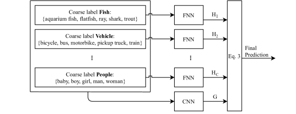
Figure 1: Pipeline of the proposed HAR network design to improve hierarchical adversarial robustness of the neural network. The final prediction of the HAR network is computed using Equation 3 based on the CNN’s prediction of the coarse classes ($G(x)=\left[g_{1},\dotsc,g_{\text{c}}\right]$) and the FNNs’ prediction of the fine classes ($H_{i}(x),\dotsc,H_{c}(x)$).

3.1 Architecture Design of HAR

Instead of the traditional flat design of the neural network, HAR consists of one CNN for the coarse labels and several FNNs for the fine labels. Note that there is a one-to-one correspondence between a particular FNN and a specific group of fine labels. Such a module design mimics the hierarchical structure of the dataset where the fine classes are grouped into coarse classes. Recall that our definition of the neural network $F(x)$ includes the softmax function as its last layer, so the output of the network can be interpreted as the probability distribution of the classes: $P(y\mid x)$. Conditioned on the probability of the coarse class, we can define the fine class probability as

$$P(y\mid x)=P(y\mid x,z)P(z\mid x).$$ (2)

Here, the probability distribution of the fine classes are computed as the product of two terms. Given an input $x$, the first term $P(y\mid x,z)$ represents the probability of $x$ being a fine label $y$ where $y$ belongs to a coarse class $z$. This is essentially FNNs’ prediction of the fine classes within a coarse category. The second term $P(z\mid x)$ represents the probability of $x$ being a coarse label $z$, and it can be understood as the prediction from the CNN. With this decomposition of the original learning task, we can reconstruct the fine label distribution by probabilistically combining the predictions from the different networks.

An important advantage of this flexible modular network design is that it allows us to train the component networks using adversarial defence techniques to improve the robustness of their associated task. Especially, a robustified coarse neural network leads to improved hierarchical adversarial robustness between coarse labels. During training, each component of the HAR network is trained independently, allowing them to be trained in parallel. We use the entire dataset with the coarse labels, $\left\{x,z\right\}$, to train the coarse class network $G(x)$, followed by training multiple fine class network $H(x)$ using only a portion of the dataset.

The inference procedure can be described as follows. Suppose the number of coarse classes in a dataset is $C$, and each coarse class contains $j$ number of fine classes. Similar to the definition of $F(x)$, we use $G(x)$ to denote the output of the CNN: $G(x)=\left[g_{1},\dotsc,g_{\text{c}}\right]$. We use $H_{i}(x)$ to denote the output of the FNN: $H_{i}(x)=\left[h_{1}^{i},\dotsc,h_{j}^{i}\right]$, where $j$ is an positive integer indicating the number of fine classes in the coarse class $i$. In this setting, the output of the combined neural network is:

$$F(x)=\left[g_{1}H_{1}(x),\dotsc,g_{\text{C}}H_{\text{C}}(x)\right].$$ (3)

3.2 Related Work on Adversarial Defence Methods

A large body of defence mechanisms have been proposed for the adversarial setting. Adversarial training (Szegedy et al., 2014) is one of the standard approaches for improving the robustness of deep neural networks against adversarial examples. It is a data augmentation method that replaces unperturbed training data with adversarial examples and updates the network with the replaced data points. Intuitively, this procedure encourages the DNN not to make the same mistakes against an adversary. By adding sufficiently enough adversarial examples, the network gradually becomes robust to the attack it was trained on. Existing adversarial training methods  (Szegedy et al., 2014; Goodfellow et al., 2015; Kurakin et al., 2017; Madry et al., 2018; Wong et al., 2019a) differ in the adversaries used in the training. Another related line of adversarial defence methods focuses on regularizing the loss function instead of data augmentation. TRADES (Zhang et al., 2019) introduces a regularization term that penalizes the difference between the output of the model on a training data and its corresponding adversarial example. The regularized loss consists of a standard cross-entropy loss on the unperturbed data and a KL-divergence term measuring the difference between the distribution of clean training data and adversarially perturbed training data.

4 Experiments

In this section, we evaluate the hierarchical adversarial robustness of the HAR network design, incorporating two popular adversarial defence methods: adversarial training with PGD10 adversaries (Madry et al., 2018) and TRADES (Zhang et al., 2019). In this section, we focus on evaluations based on $\ell_{\infty}$ norm attacks on the CIFAR-100 dataset, and defer evaluations on $\ell_{2}$ of CIFAR-100 in Appendix D. Additionally, we include evaluations on the small-sized CIFAR-10 dataset and the medium-sized CIFAR-100-5x5 dataset (a 25-class subset of CIFAR-100) in Appendix E. The result shows that the standard untargeted PGD attack is insufficient at empirically evaluating model’s hierarchical adversarial robustness, as shown by the significant drop in coarse class accuracy from the proposed worst-case targeted attack. Compared to the traditional flat design of neural network, our experiments show that HAR leads to a significant improvement in hierarchical adversarial robustness under various targeted and untargeted attacks (Section 4.2). Lastly, we show that one can generate hierarchical adversarial examples based on the CNN part of the HAR network under the white-box threat model, but they are not as strong as the proposed worst-case targeted attack in degrading model’s hierarchical robustness (Section 4.3).

4.1 Evaluation Setup

We use network architectures from the ResNet family (He et al., 2016) on the CIFAR-100 dataset. The hierarchical structure of classes within the dataset is illustrated in Table 7. To establish a baseline, we train ResNet50 networks using the following methods: (1) Standard: training with unperturbed data; (2) ADV: training with 10-step untargeted PGD examples (3) ADV-T: training with 10-step randomly targeted PGD examples (4) TRADES and (5) ADV-hCE: training with 10-step untargeted PGD examples based on a modified hierarchical cross-entropy (hCE) loss.

To further justify the use of separate networks for the coarse and fine classification tasks in HAR, we compare with two natural baselines. ADV-T is a targeted-variant of the PGD adversarial training in Madry et al. (2018). Specifically, given a pair of input from the training set $(x,y)$ and $y\in z^{*}$, the perturbation is computed based on a targeted 10-step PGD attack where the target label is uniformly random sampled from $\{y\mid y\not\in z^{*}\}$. An alternative to HAR is to train a single flat network with a modified hierarchical loss. The idea of incorporating hierarchical structure in losses has been explored in the literature (Cesa-Bianchi et al., 2006; Redmon and Farhadi, 2017; Ge, 2018; Wehrmann et al., 2018), but not yet studied under the robust learning setting. As such, we performed ADV-hCE, i.e., adversarial training using a hierarchical cross-entropy loss: $\ell_{\text{hCE}}(x,y,z)\triangleq\ell(F(x),y)+\ell(G(x),z)$ where $F(x)$ is the prediction of the network of the fine classes. $G(x)$ is the predictions of the coarse classes and its entries are computed by summing the corresponding fine class predictions in $F(x)$.

To differentiate HAR networks from the flat models, we refer the flat models as vanilla models. We use a single ResNet50 for the vanilla model. For the proposed HAR network, we use multiple ResNet10 for the coarse network and the fine networks. We use individual models with a lower capacity for HAR to reduce the difference in the order of magnitude of parameters between a single ResNet50 in the vanilla model and multiple ResNet10 in HAR. Notice that in the experiment with CIFAR-10 and CIFAR-100-5x5, the number of trainable parameters of the vanilla model is larger than that of the HAR network using the selected ResNet architectures. While this is difficult to achieve with CIFAR-100, the goal here is to eliminate the concern of which the improved hierarchical adversarial robustness is obtained solely due to the increasing network complexity. A comparison between the number of trainable parameters is included in Appendix A. Note that in the HAR network, all component networks (CNN and FNNs) are trained using the same adversarial defence approach. As a concrete example, a HAR network trained with TRADES on CIFAR-100 consists of one coarse classifier and twenty fine classifiers where they are all trained using TRADES.

For all five methods (Standard, ADV, ADV-T, ADV-hCE and TRADES), networks are trained for a total of 200 epochs, with an initial learning rate of 0.1. The learning rate decays by an order of magnitude at epoch 100 and 150. We used a minibatch size of 128 for testing and training. We used SGD optimizer with momentum of 0.9 and a weight decay of 2e-4. For TRADES, we performed a hyperparameter sweep on the strength of the regularization term $\beta$ and selected one that resulted in the highest accuracy against untargeted $\ell_{\infty}$ bounded PGD20 attacks. The optimization procedure is used for both the vanilla models and all component models in the HAR network.

Table 2: Accuracy of different models on CIFAR-100 against $\ell_{\infty}$ bounded white-box untargeted PGD attacks.

Method		Clean		PGD20 (${\epsilon}=\frac{4}{255}$)		PGD20 (${\epsilon}=\frac{8}{255}$)
		Fine	Coarse	Fine	Coarse	Fine	Coarse
Vanilla	Standard	$73.21\%$	$82.57\%$	$0.01\%$	$24.89\%$	$0.01\%$	$24.89\%$
	ADV	$58.62\%$	$69.81\%$	$21.36\%$	$37.80\%$	$21.36\%$	$37.80\%$
	ADV-T	$64.74\%$	$75.02\%$	$17.19\%$	$41.30\%$	$17.19\%$	$41.30\%$
	TRADES	$57.12\%$	$67.67\%$	$26.69\%$	$41.47\%$	$26.69\%$	$41.47\%$
HAR	Standard	$63.49\%$	$81.24\%$	$0.12\%$	$29.25\%$	$0.12\%$	$29.25\%$
	ADV	$48.53\%$	$66.23\%$	$20.28\%$	$30.53\%$	$22.28\%$	$30.53\%$
	TRADES	$46.62\%$	$62.49\%$	$22.00\%$	$32.86\%$	$22.00\%$	$32.86\%$

Method		PGD50 (${\epsilon}=\frac{8}{255}$)		PGD100 (${\epsilon}=\frac{8}{255}$)		PGD200 (${\epsilon}=\frac{8}{255}$)
		Fine	Coarse	Fine	Coarse	Fine	Coarse
Vanilla	Standard	$0.01\%$	$24.84\%$	$0.00\%$	$25.12\%$	$0.01\%$	$24.94\%$
	ADV	$21.05\%$	$37.16\%$	$20.87\%$	$36.96\%$	$20.94\%$	$37.02\%$
	ADV-T	$16.94\%$	$41.07\%$	$16.88\%$	$40.99\%$	$16.79\%$	$40.84\%$
	TRADES	$26.48\%$	$41.22\%$	$26.58\%$	$41.40\%$	$26.52\%$	$41.27\%$
HAR	Standard	$0.15\%$	$28.91\%$	$0.14\%$	$29.46\%$	$0.15\%$	$29.27\%$
	ADV	$19.91\%$	$29.94\%$	$20.03\%$	$29.99\%$	$19.89\%$	$29.93\%$
	TRADES	$21.99\%$	$32.66\%$	$21.90\%$	$32.60\%$	$21.87\%$	$32.36\%$

Table 3: Accuracy of different models on CIFAR-100 against $\ell_{\infty}$ bounded worst-case targeted PGD attacks based on Algorithm 1.

Method		PGD20	PGD20	PGD50	PGD100	PGD200
		(${\epsilon}=\frac{4}{255}$)	(${\epsilon}=\frac{8}{255}$)	(${\epsilon}=\frac{8}{255}$)	(${\epsilon}=\frac{8}{255}$)	(${\epsilon}=\frac{8}{255}$)
Vanilla	Standard	$0.00\%$	$0.00\%$	$0.00\%$	$0.00\%$	$0.00\%$
	ADV	$43.30\%$	$24.60\%$	$24.60\%$	$24.50\%$	$24.00\%$
	ADV-T	$43.50\%$	$22.10\%$	$21.70\%$	$20.70\%$	$21.00\%$
	TRADES	$47.20\%$	$30.00\%$	$29.80\%$	$29.70\%$	$28.80\%$
HAR	Standard	$8.60\%$	$4.00\%$	$3.50\%$	$3.40\%$	$3.30\%$
	ADV	$\bm{43.70}\%$	$\bm{25.80}\%$	$\bm{25.50}\%$	$\bm{25.30}\%$	$\bm{24.40}\%$
	TRADES	$45.80\%$	$29.20\%$	$28.90\%$	$29.30\%$	$\bm{28.90}\%$

4.2 Hierarchical Robustness under Untargeted and Targeted Attacks

There are several threat models to consider while evaluating adversarial robustness, regardless of standard or hierarchical robustness. The white-box threat model specifies that the model architecture and network parameters are fully transparent to the attacker  (Goodfellow et al., 2015). Despite many white-box attack methods exist, perturbations generated using iterations of PGD remain as one of the most common benchmarks for evaluating adversarial robustness under the white-box setting. Specifically, we perform 20, 50, 100 and 200 iterations of PGD on the entire test set data for the untargeted attacks in Table 2. To evaluate the hierarchical robustness of the model, we perform the worst-case hierarchical adversarial perturbations introduced in Section 2.2. Due to the large number of fine labels in CIFAR-100, the hierarchical attack was performed on 1000 randomly selected test set data. All $\ell_{\infty}$-PGD adversarial examples used for all evaluations are generated a step size of ${\epsilon}/4$ (pixel values are normalized to $[0,1]$).

Along with the two attacks, we also include results on unperturbed testset data (Clean). For clean and untargeted attacks, we report the percentage of correct fine class prediction as fine accuracy, and the percentage of fine class prediction belonging to the correct coarse class as coarse accuracy. For the proposed targeted attack reported in Table 3, the accuracy refers to the percentage of the test set data where the targeted attack fails to alter the final prediction to the desired target, even after iterating through all eligible target labels. It is important to realize that a successful targeted attack implies misclassification for both coarse and fine classes.

4.2.1 Discussions

Before making the comparison between the HAR model and the vanilla model, we make an interesting observation in Table 2: there is a consistent gap between the fine and coarse accuracy for both clean and perturbed inputs. This shows that under the untargeted attack, some of the misclassified inputs at the fine level are actually still classified correctly at the coarse level. In particular, vanilla networks trained with unperturbed training data have close to $0\%$ fine accuracy under untargeted PGD attacks with ${\epsilon}=8/255$, while nearly $25\%$ of all the misclassified inputs still belong to the correct coarse class. This shows that the untargeted attacks do not provide a good representation of the hierarchical adversarial robustness as an empirical evaluation, and it supports our earlier observation in Section 2.1 which is the main drive for the proposal of a targeted attack specifically designed for reducing coarse accuracy and damaging hierarchical robustness.

Indeed, results in Table 3 show that the proposed worst-case targeted attack severely damages the hierarchical adversarial robustness of all models. On Standard trained models, despite the high hierarchical robustness under untargeted attacks, nearly all of the CIFAR-100 data can be perturbed into a desired target class from another coarse class. Therefore, we emphasize the use of the proposed worst-case targeted attack for a more accurate empirical evaluations for the hierarchical adversarial robustness of the model. For vanilla models trained with ADV and TRADES, we notice that the improved adversarial robustness on fine classes translates to an improvement in hierarchical adversarial robustness.

The result shows that ADV-hCE does not outperform the standard ADV in hierarchical robustness, and thus, we defer its discussions in Appendix F. We discuss ADV-T here, as it serves an excellent case to emphasize that since evaluating robustness empirically using attacks only shows an upper bound on the true robustness of the model, one should focus on the metric that results in the lowest upper bound. For this reason, a network outperforming another on weaker metrics does not imply it has better hierarchical robustness. With this notion, we observed that vanilla models trained using ADV-T shows improved hierarchical robustness against untargeted PGD attacks compared to the original adversarial training method. However, results in Table 3 suggests that the seeming improvement in hierarchical robustness of the ADV-T method does not hold against stronger hierarchical attacks. ADV-trained models outperform ADV-T models on all targeted PGD attacks with ${\epsilon}=8/255$.

Finally, the result shows that ADV-trained HAR network significantly improves the hierarchical robustness against all worst-case targeted attacks compared to the vanilla counterpart. Particularly, we notice a $0.4\%$ increase in accuracy against PGD200 adversaries. For TRADES-robusitified networks, we observe that although the vanilla model outperforms HAR against weaker targeted adversaries (i.e., smaller ${\epsilon}$ and small PGD iterations), the gain in hierarchical robustness with HAR rises as the targeted attack becomes stronger. For the strongest PGD200 attack, we notice a $0.1\%$ increase in accuracy compared to the vanilla model.

4.3 Hierarchical Robustness under Targeted Attacks based on the Coarse Network

Under the white-box threat model, attackers with a complete knowledge of the internal structure of HAR can also generate perturbations based on the coarse network. During evaluations, we investigate whether the targeted PGD adversaries based on the coarse network are stronger hierarchical adversarial examples compared to the ones generated using the entire network. Such attacks can be understood as finding a more general perturbation which alters the probability distribution of the coarse class: $P(z\mid x)$. Similar to the attack proposed in Section 2.2, we perform an iterative, worst-case targeted PGD20 attack based on the coarse neural network. Specifically, we replace $\ell(F(x),y)$ with $\ell(G(x),z)$ in Equation 1, and iterate through all eligible coarse classes as target labels. For example, to generate such attacks for HAR with ADV-trained component networks, the iterative targeted attack is performed based on the ADV-trained coarse network in the original HAR network. Note that there is a distinction between the above attack procedure and a transfer-based attack where the perturbation is transferred from an independently trained source model (Papernot et al., 2017). Since the perturbation is generated using part of the HAR network, such attacks still belongs in the white-box setting. Results in Table 4 show that the perturbations generated using the coarse network are weaker attacks compared to the ones generated using the entire HAR network.

Table 4: Accuracy of the HAR network on CIFAR-100 against $\ell_{\infty}$ bounded targeted attacks (${\epsilon}=8/255$) generated using the coarse network (Coarse). For comparison, the untargeted attack (PGD200 from Table 2) and the attack generated using the entire HAR network (PGD200 from Table 3) are also included.

Method	Untargeted	Coarse	HAR
Standard	$29.27\%$	$\bm{0.00}\%$	$3.30\%$
ADV	$29.93\%$	$29.96\%$	$\bm{24.40}\%$
TRADES	$32.36\%$	$29.38\%$	$\bm{28.90}\%$

5 Conclusion

In this work, we introduced a novel concept called hierarchical adversarial examples. For dataset which classes can be further categorized into fine and coarse classes, we defined hierarchical adversarial examples as the ones leading to a misclassification at the coarse level. We proposed a worst-case targeted PGD attack to generate hierarchical adversarial examples. To improve the hierarchical adversarial robustness of DNNs, we proposed the HAR network design, a composite of a coarse network and fine networks where each component network is trained independently by adversarial defence techniques. We empirically showed that HAR leads to a significant increase in hierarchical adversarial robustness on CIFAR-10 and CIFAR-100.

The rapid adoption of machine learning applications has also led to an increasing importance in improving the robustness and reliability of such techniques. Mission-critical and safety-critical systems which rely on DNNs in their decision-making process shall incorporate robustness, along with accuracy, in the development process. The introduction of the hierarchical adversarial examples and ways to defend against them is an important step towards a more safe and trustworthy AI system.

Appendix A Comparison of trainable model parameters

In our evaluations with CIFAR-100, we use ResNet50 for the vanilla models and multiple ResNet10 for the HAR network. Note that we use architectures with a lower capacity for the individual components in HAR to reduce the difference in the order of magnitude of parameters between a single ResNet50 model and multiple ResNet10 models. For the evaluation with CIFAR-10, we use ResNet34 for the vanilla models, and use multiple ResNet10 for the HAR network. For the evaluation with CIFAR-100-5x5, we use ResNet50 for the vanilla models, and use multiple ResNet10 for the HAR network. In those two cases, the number of trainable parameters of the vanilla model is larger than that of the HAR network. While this is difficult to achieve with CIFAR-100 given its large number of coarse labels, the goal here is to address the concern of which the improved hierarchical adversarial robustness is obtained only due to the increasing network complexity.

Table 5: Number of trainable parameters in the ResNet architectures used in our evaluations

Model	Number of Parameters
ResNet10	$4.9$ M
ResNet34	$21.3$ M
ResNet50	$25.6$ M

Appendix B Hyperparameter sweep for TRADES on ResNet10

An important hyperparameter in training with TRADES (Zhang et al., 2019) is $\beta$ which balances the trade-off between standard accuracy on the clean data and the robust accuracy on the perturbed one. In Zhang et al. (2019), the sweep of $\beta$ was only performed on more complex models such as WideResNet. As such, we performed a similar hyperparameter sweep to determine the optimal $\beta$ in TRADES on ResNet10 using the CIFAR-10 dataset. In Table 6, we compared the standard accuracy and the robust accuracy of models trained using TRADES with various value of $\beta$. The FGSM and the untargeted PGD20 perturbations are $\ell_{\infty}$ bounded with (${\epsilon}=\frac{8}{255}$). Based on the result, we used $\beta$ of value $9$ while training with TRADES in our evaluations as it resulted in the highest untargeted PGD20 accuracy. We emphasize the main goal of the paper is to demonstrate the novel concept of hierarchical adversarial robustness including techniques to generate and defend against them, rather than reaching for SOTA performance. Therefore, fine-tuning the optimization parameters including the $\beta$ for the CIFAR-100-5x5 and CIFAR-100 datasets would not be necessary and we simply used the same $\beta$ for the two datasets.

Table 6: Hyperparameter sweep of TRADES on ResNet10 using CIFAR-10. The FGSM and PGD20 perturbations are $\ell_{\infty}$ bounded with (${\epsilon}=\frac{8}{255}$). We used $\beta$ of value $9$ while training with TRADES in the evaluations as it resulted in the highest untargeted PGD20 accuracy.

$\beta$	Clean	FGSM	PGD20
15	$72.80\%$	$48.85\%$	$44.80\%$
13	$73.46\%$	$49.18\%$	$45.09\%$
11	$74.46\%$	$49.39\%$	$44.86\%$
9	$75.61\%$	$\bm{50.06}\%$	$\bm{45.38}\%$
7	$76.74\%$	$50.05\%$	$45.04\%$
5	$78.39\%$	$50.22\%$	$44.40\%$
3	$80.20\%$	$49.84\%$	$42.53\%$
1	$83.69\%$	$45.61\%$	$35.27\%$
0.5	$84.00\%$	$46.16\%$	$34.40\%$
0.1	$\bm{84.64}\%$	$41.12\%$	$16.52\%$

Appendix C Hierarchical structure of classes within the CIFAR-10 dataset

To demonstrate the effectiveness of the proposed hierarchical attack in Section 2.2 and the improved hierarchical robustness with HAR, we performed an extensive empirical study on three datasets: the small-sized CIFAR-10 dataset with 2 coarse classes and 10 fine classes, the medium-sized CIFAR-100-5x5 dataset with 5 coarse classes and 25 fine classes, and the large-sized CIFAR-100 dataset with 20 coarse classes and 100 fine classes. The hierarchical structure of the datasets are shown in Table 7.

Table 7: The hierarchical structure of classes within the CIFAR-10, CIFAR-100-5x5 and CIFAR-100 dataset

	Coarse labels	Fine labels
CIFAR-10	Animals	bird, cat, deer, dog, frog, horse
	Vehicles	airplane, automobile, ship, truck
CIFAR-100-5x5	Fish	aquarium fish, flatfish, ray, shark, trout
	Vehicles	bicycle, bus, motorcycle, pickup truck, train
	People	baby, boy, girl, man, woman
	Trees	maple, oak, palm, pine, willow
	Insects	bee, beetle, butterfly, caterpillar, cockroach
CIFAR-100	Aquatic mammals	beaver, dolphin, otter, seal, whale
	Fish	aquarium fish, flatfish, ray, shark, trout
	Flowers	orchids, poppies, roses, sunflowers, tulips
	Food containers	bottles, bowls, cans, cups, plates
	Fruit and vegetables	apples, mushrooms, oranges, pears, sweet peppers
	Household electrical devices	clock, computer keyboard, lamp, telephone, television
	Household furniture	bed, chair, couch, table, wardrobe
	Insects	bee, beetle, butterfly, caterpillar, cockroach
	Large carnivores	bear, leopard, lion, tiger, wolf
	Large man-made outdoor things	bridge, castle, house, road, skyscraper
	Large natural outdoor scenes	cloud, forest, mountain, plain, sea
	Large omnivores and herbivores	camel, cattle, chimpanzee, elephant, kangaroo
	Medium-sized mammals	fox, porcupine, possum, raccoon, skunk
	Non-insect invertebrates	crab, lobster, snail, spider, worm
	People	baby, boy, girl, man, woman
	Reptiles	crocodile, dinosaur, lizard, snake, turtle
	Small mammals	hamster, mouse, rabbit, shrew, squirrel
	Trees	maple, oak, palm, pine, willow
	Vehicles 1	bicycle, bus, motorcycle, pickup truck, train
	Vehicles 2	lawn-mower, rocket, streetcar, tank, tractor

Appendix D Results on CIFAR-100 with $\ell_{2}$ bounded attacks

In this section, we empirically study the effectiveness of the $\ell_{2}$ bounded hierarchical attack and the improved hierarchical robustness from HAR. The $\ell_{2}$ bounded worts-case targeted PGD attack is formulated in a similar fashion as the one illustrated in Algorithm 1 and the only difference is that the perturbation generated at each iteration of PGD is ensured to be within the $\ell_{2}$-ball of the original input. Additionally, due to the large number of fine labels in CIFAR-100, the hierarchical attack was performed on 1000 randomly selected test set data. Similar to the setup with $\ell_{\infty}$ attacks in Section 4.2, we compare various baselines where the model is robustified against $\ell_{2}$ attacks. Note that we were not able to achieve reasonable robustness results with TRADES against $\ell_{2}$ attacks. One possible reason is that the hyperparameter sweep was based on the $\ell_{\infty}$ results, as such, the optimal value for $\beta$ is unsuitable in the $\ell_{2}$ setting. For this reason, we omit TRADES in this section.

Similar to Section 4.2, we make two important observations. First, we notice that the lowest coarse accuracy for the untargeted PGD attack (${\epsilon}=0.5$) is $53.59\%$ and $48.91\%$ respectively for the ADV-trained vanilla model and the HAR network. In Table 9, we observe that the proposed worst-case targeted PGD attack severely degrades the coarse accuracy for both models. In particular, for the vanilla model, the proposed attack results in a $10\%$ decrease in coarse accuracy. This matches the result with $\ell_{\infty}$ attacks in Section 4.2 and it shows that the proposed worst-case targeted PGD attack provides a more accurate empirical representation of the hierarchical adversarial robustness of the model. Next, we observe that the targeted adversarial training does not improve the hierarchical robustness compared to the standard adversarial training, and ADV-trained HAR network improves the hierarchical adversarial robustness. Particularly, we observe a $1.1\%$ improvement in the hierarchical robustness against $\ell_{2}$ bounded worst-case targeted attacks with the HAR design in comparison to the vanilla network.

Table 8: Accuracy of different models on CIFAR-100 against $\ell_{2}$ bounded white-box untargeted PGD attacks. (a higher score indicates better performance)

Method		Clean		PGD20 (${\epsilon}=0.25$)		PGD20 (${\epsilon}=0.5$)
		Fine	Coarse	Fine	Coarse	Fine	Coarse
Vanilla	Standard	$73.21\%$	$82.57\%$	$3.05\%$	$35.95\%$	$0.29\%$	$31.86\%$
	ADV	$64.38\%$	$74.85\%$	$50.04\%$	$64.05\%$	$36.35\%$	$53.77\%$
	ADV-T	$68.73\%$	$78.58\%$	$48.78\%$	$64.62\%$	$31.41\%$	$53.10\%$
HAR	ADV	$56.96\%$	$73.31\%$	$43.87\%$	$60.68\%$	$31.91\%$	$48.94\%$

Method		PGD50 (${\epsilon}=0.5$)		PGD100 (${\epsilon}=0.5$)		PGD200 (${\epsilon}=0.5$)
		Fine	Coarse	Fine	Coarse	Fine	Coarse
Vanilla	Standard	$0.17\%$	$32.17\%$	$0.13\%$	$32.55\%$	$0.12\%$	$32.07\%$
	ADV	$36.16\%$	$53.64\%$	$36.11\%$	$53.61\%$	$36.07\%$	$53.59\%$
	ADV-T	$31.21\%$	$52.97\%$	$31.15\%$	$52.82\%$	$31.09\%$	$52.78\%$
HAR	ADV	$31.90\%$	$48.78\%$	$31.76\%$	$48.70\%$	$31.70\%$	$48.91\%$

Table 9: Accuracy of different models on CIFAR-100 against $\ell_{2}$ bounded worst-case targeted PGD attacks. (a higher score indicates better performance)

Method		PGD20	PGD50
		(${\epsilon}=0.5$)	(${\epsilon}=0.5$)
Vanilla	Standard	$0.10\%$	$0.10\%$
	ADV	$43.60\%$	$42.90\%$
	ADV-T	$39.20\%$	$38.50\%$
HAR	ADV	$\bm{44.30}\%$	$\bm{44.00}\%$

Appendix E Results on CIFAR-10 and CIFAR-100-5x5 with $\ell_{\infty}$ bounded attacks

In this section, we examine the $\ell_{\infty}$ bounded hierarchical attack and the improved hierarchical robustness from HAR on the small-sized CIFAR-10 with 2 coarse classes and 10 fine classes, and the medium-sized CIFAR-100-5x5 with 5 coarse classes and 25 fine classes. In Table 10, we compare the HAR network to vanilla baselines using the accuracy on clean data, untargeted PGD20 adversaries and the targeted PGD hierarchical attack proposed in Section 2.2. We observe that HAR network trained with ADV and TRADES significantly improves the robustness against the worst-case targeted attacks compared to the vanilla counterparts. On CIFAR-10, HAR network achieves a $7.52\%$ and $1.47\%$ improvement when trained with ADV and TRADES respectively. On CIFAR-100-5x5, we observe a drastic improvement in hierarchical robustness using HAR: with more than $10\%$ increase in resistance to the worst-case targeted attacks compared to the vanilla models.

Table 10: Performance on CIFAR-10 and CIFAR-100-5x5 against $\ell_{\infty}$ bounded attacks (${\epsilon}=8/255$): the untargeted PGD20 attacks (Untargeted) and the worst-case targeted hierarchical attacks (Targeted). (a higher score indicates better model robustness against specific attacks)

	Method		Clean		Untargeted		Targeted
			Fine	Coarse	Fine	Coarse
CIFAR-10	Vanilla	Standard	$92.88\%$	$98.93\%$	$0.00\%$	$\underline{79.73\%}$	$0.00\%$
		ADV	$84.31\%$	$97.49\%$	$47.65\%$	$87.40\%$	$72.00\%$
		TRADES	$79.70\%$	$95.69\%$	$48.89\%$	$88.15\%$	$79.76\%$
	HAR	Standard	$92.19\%$	$98.44\%$	$0.00\%$	$\underline{65.46\%}$	$0.00\%$
		ADV	$79.80\%$	$95.57\%$	$43.82\%$	$86.38\%$	$\bm{79.52\%}$
		TRADES	$77.78\%$	$94.49\%$	$46.75\%$	$86.07\%$	$\bm{81.23\%}$
CIFAR-100-5x5	Vanilla	Standard	$72.80\%$	$92.68\%$	$0.00\%$	$\underline{65.52\%}$	$0.00\%$
		ADV	$61.96\%$	$86.08\%$	$24.12\%$	$70.68\%$	$42.20\%$
		TRADES	$59.28\%$	$84.16\%$	$28.36\%$	$69.60\%$	$48.04\%$
	HAR	Standard	$67.12\%$	$94.36\%$	$3.71\%$	$\underline{56.72\%}$	$0.11\%$
		ADV	$57.48\%$	$89.16\%$	$25.80\%$	$63.32\%$	$\bm{52.32\%}$
		TRADES	$55.44\%$	$84.96\%$	$32.80\%$	$66.36\%$	$\bm{58.96\%}$

Appendix F Hierarchical cross-entropy loss

To further justify the use of separate networks for the robust hierarchical classification tasks in HAR, we compare two additional two baselines. In Section 4.2, we showed that the improvement in hierarchical robustness of the ADV-T trained vanilla models does not hold against stronger hierarchical attacks. Another alternative to using separate networks is to train a single flat network with a modified hierarchical loss. The idea of incorporating hierarchical structure in losses has been explored in the literature (Cesa-Bianchi et al., 2006; Redmon and Farhadi, 2017; Ge, 2018; Wehrmann et al., 2018), but not yet studied under the robust learning setting. As such, we proposed ADV-hCE, i.e., adversarial training using a hierarchical cross-entropy loss. First, we define the hierarchical cross-entropy loss as

$$\ell_{\text{hCE}}(x,y,z)\triangleq\ell(F(x),y)+\ell(G(x),z),$$ (4)

where $F(x)$ and $G(x)$ are the predictions of the fine classes and coarse classes respectively. In particular, $F(x)$ is the output of the neural network and entries in $G(x)$ are computed by summing the corresponding fine class predictions in $F(x)$. For example, suppose we have four fine classes and two coarse classes and, given an input, the prediction of the network is $F(x)=[0.2,0.4,0.3,0.1]$. If the first two entries in $F(x)$ correspond to the same coarse classes, then we have $G(x)=[0.6,0.4]$. Intuitively, the second term in the hierarchical cross-entropy loss can be understood as a penalty for assigning probabilities of fine labels outside of the correct coarse class. As such, we trained two flat ResNet10 models on the CIFAR-10 dataset using adversarial training based on the cross-entropy loss and the hierarchical cross-entropy loss respectively. It is important to realize that since adversarial training involves replacing the clean training data with the perturbed data, this means the PGD adversaries used during ADV-hCE are generated based on the hierarchical cross-entropy loss. We observe that although models trained using the modified loss shows improved hierarchical robustness against untargeted PGD attacks generated from both the original and the hierarchical cross-entropy loss. However, such an improvement in hierarchical robustness does not hold against stronger targeted hierarchical attacks, captured by the $50\%$ drop in accuracy against the worst-case targeted attack.

Table 11: Accuracy of the model trained with the hierarchical cross-entropy loss on CIFAR-10 against $\ell_{\infty}$ bounded attacks (${\epsilon}=8/255$): the untargeted PGD20 attacks based on the cross-entropy loss (Untargeted-CE), the untargeted PGD20 attacks based on the hierarchical cross-entropy loss (Untargeted-hCE) and the proposed worst-case hierarchical attack (Targeted).

Method	Clean		Untargeted-CE		Untargeted-hCE		Targeted
	Fine	Coarse	Fine	Coarse	Fine	Coarse
ADV-CE	$78.38\%$	$91.57\%$	$39.68\%$	$84.11\%$	$42.10\%$	$77.97\%$	$77.44\%$
ADV-hCE	$74.89\%$	$95.56\%$	$38.26\%$	$87.4\%$	$39.56\%$	$81.12\%$	$22.34\%$

References

- Carlini and Wagner (2017) Nicholas Carlini and David Wagner. Towards evaluating the robustness of neural networks. In 2017 ieee symposium on security and privacy (sp), pages 39–57. IEEE, 2017.
- Cesa-Bianchi et al. (2006) Nicolo Cesa-Bianchi, Claudio Gentile, and Luca Zaniboni. Incremental algorithms for hierarchical classification. The Journal of Machine Learning Research, 7:31–54, 2006.
- Cordts et al. (2016) Marius Cordts, Mohamed Omran, Sebastian Ramos, Timo Rehfeld, Markus Enzweiler, Rodrigo Benenson, Uwe Franke, Stefan Roth, and Bernt Schiele. The cityscapes dataset for semantic urban scene understanding. In Proceedings of the IEEE conference on computer vision and pattern recognition, pages 3213–3223, 2016.
- Croce and Hein (2020) Francesco Croce and Matthias Hein. Reliable evaluation of adversarial robustness with an ensemble of diverse parameter-free attacks. In International Conference on Machine Learning, pages 2206–2216. PMLR, 2020.
- Deng et al. (2009) Jia Deng, Wei Dong, Richard Socher, Li-Jia Li, Kai Li, and Li Fei-Fei. Imagenet: A large-scale hierarchical image database. In 2009 IEEE conference on computer vision and pattern recognition, pages 248–255. Ieee, 2009.
- Deng et al. (2011) Jia Deng, Sanjeev Satheesh, Alexander C Berg, and Fei Li. Fast and balanced: Efficient label tree learning for large scale object recognition. In Advances in Neural Information Processing Systems, pages 567–575, 2011.
- Deng et al. (2012) Jia Deng, Jonathan Krause, Alexander C Berg, and Li Fei-Fei. Hedging your bets: Optimizing accuracy-specificity trade-offs in large scale visual recognition. In 2012 IEEE Conference on Computer Vision and Pattern Recognition, pages 3450–3457. IEEE, 2012.
- Everingham et al. (2015) Mark Everingham, SM Ali Eslami, Luc Van Gool, Christopher KI Williams, John Winn, and Andrew Zisserman. The pascal visual object classes challenge: A retrospective. International journal of computer vision, 111(1):98–136, 2015.
- Ge (2018) Weifeng Ge. Deep metric learning with hierarchical triplet loss. In Proceedings of the European Conference on Computer Vision (ECCV), pages 269–285, 2018.
- Geiger et al. (2013) Andreas Geiger, Philip Lenz, Christoph Stiller, and Raquel Urtasun. Vision meets robotics: The kitti dataset. The International Journal of Robotics Research, 32(11):1231–1237, 2013.
- Goodfellow et al. (2015) Ian J Goodfellow, Jonathon Shlens, and Christian Szegedy. Explaining and harnessing adversarial examples. In International Conference on Learning Representations, 2015.
- Gowal et al. (2019) Sven Gowal, Jonathan Uesato, Chongli Qin, Po-Sen Huang, Timothy Mann, and Pushmeet Kohli. An alternative surrogate loss for pgd-based adversarial testing. arXiv preprint arXiv:1910.09338, 2019.
- Hastie et al. (2009) Trevor Hastie, Robert Tibshirani, and Jerome Friedman. The Elements of Statistical Learning: Data Mining, Inference, and Prediction (2nd edition). Springer, 2009.
- He et al. (2016) Kaiming He, Xiangyu Zhang, Shaoqing Ren, and Jian Sun. Deep residual learning for image recognition. In Proceedings of the IEEE conference on computer vision and pattern recognition, pages 770–778, 2016.
- Krizhevsky (2009) Alex Krizhevsky. Learning multiple layers of features from tiny images. 2009.
- Kurakin et al. (2017) Alexey Kurakin, Ian Goodfellow, and Samy Bengio. Adversarial machine learning at scale. In International Conference on Learning Representations, 2017.
- Li et al. (2003) Beitao Li, Edward Chang, and Yi Wu. Discovery of a perceptual distance function for measuring image similarity. Multimedia systems, 8(6):512–522, 2003.
- Liu et al. (2013) Baoyuan Liu, Fereshteh Sadeghi, Marshall Tappen, Ohad Shamir, and Ce Liu. Probabilistic label trees for efficient large scale image classification. In Proceedings of the IEEE conference on computer vision and pattern recognition, pages 843–850, 2013.
- Madry et al. (2018) Aleksander Madry, Aleksandar Makelov, Ludwig Schmidt, Dimitris Tsipras, and Adrian Vladu. Towards deep learning models resistant to adversarial attacks. In International Conference on Learning Representations, 2018.
- Mao et al. (2021) Xiaofeng Mao, Yuefeng Chen, Shuhui Wang, Hang Su, Yuan He, and Hui Xue. Composite adversarial attacks. In Proceedings of the AAAI Conference on Artificial Intelligence, 2021.
- Marszałek and Schmid (2008) Marcin Marszałek and Cordelia Schmid. Constructing category hierarchies for visual recognition. In European conference on computer vision, pages 479–491. Springer, 2008.
- Papernot et al. (2017) Nicolas Papernot, Patrick McDaniel, Ian Goodfellow, Somesh Jha, Z Berkay Celik, and Ananthram Swami. Practical black-box attacks against machine learning. In Proceedings of the 2017 ACM on Asia conference on computer and communications security, pages 506–519, 2017.
- Redmon and Farhadi (2017) Joseph Redmon and Ali Farhadi. Yolo9000: better, faster, stronger. In Proceedings of the IEEE conference on computer vision and pattern recognition, pages 7263–7271, 2017.
- Szegedy et al. (2014) Christian Szegedy, Wojciech Zaremba, Ilya Sutskever, Joan Bruna, Dumitru Erhan, Ian Goodfellow, and Rob Fergus. Intriguing properties of neural networks. In International Conference on Learning Representations, 2014.
- Szegedy et al. (2017) Christian Szegedy, Sergey Ioffe, Vincent Vanhoucke, and Alexander Alemi. Inception-v4, inception-resnet and the impact of residual connections on learning. In Proceedings of the AAAI Conference on Artificial Intelligence, volume 31, 2017.
- Tashiro et al. (2020) Yusuke Tashiro, Yang Song, and Stefano Ermon. Diversity can be transferred: Output diversification for white-and black-box attacks. Advances in Neural Information Processing Systems, 33, 2020.
- Tousch et al. (2012) Anne-Marie Tousch, Stéphane Herbin, and Jean-Yves Audibert. Semantic hierarchies for image annotation: A survey. Pattern Recognition, 45(1):333–345, 2012.
- Wehrmann et al. (2018) Jonatas Wehrmann, Ricardo Cerri, and Rodrigo Barros. Hierarchical multi-label classification networks. In International Conference on Machine Learning, pages 5075–5084. PMLR, 2018.
- Wong et al. (2019a) Eric Wong, Leslie Rice, and J Zico Kolter. Fast is better than free: Revisiting adversarial training. In International Conference on Learning Representations, 2019a.
- Wong et al. (2019b) Eric Wong, Frank Schmidt, and Zico Kolter. Wasserstein adversarial examples via projected sinkhorn iterations. In International Conference on Machine Learning, pages 6808–6817. PMLR, 2019b.
- Zhang et al. (2019) Hongyang Zhang, Yaodong Yu, Jiantao Jiao, Eric Xing, Laurent El Ghaoui, and Michael Jordan. Theoretically principled trade-off between robustness and accuracy. In International Conference on Machine Learning, pages 7472–7482. PMLR, 2019.