Observational evidence of fractality in the large-scale distribution of galaxies

Usando una muestra de 133 991 galaxias distribuidas en la region del cielo $100^{\circ}<\alpha<270^{\circ}$ y $7^{\circ}<\delta<65^{\circ}$ con un redshift $0.0057<z<0.12$, extraída del catálogo SDSS NASA/AMES Value Added Galaxy Catalog (AMES-VAGC), estimamos la dimensión fractal usando dos métodos. El primero usa un algoritmo para estimar la dimensión de correlación. El segundo, una nueva aproximación, crea un grafo usando los datos y estima la dimensión del grafo basado unicamente en la información de conectividad. En ambos métodos encontramos una dimensión $D\approx 2$ en escalas por debajo de 20 Mpc, lo cual concuerda con trabajos previos. Este resultado muestra la no homogeneidad de la distribución de las galaxias en ciertas escalas.

Abstract

Using a sample of 133 991 galaxies distributed in the sky region $100^{\circ}<\alpha<270^{\circ}$ and $7^{\circ}<\delta<65^{\circ}$ with a redshift $0.0057<z<0.12$, extracted from the SDSS NASA/AMES Value Added Galaxy Catalog (AMES-VAGC), we estimate the fractal dimension using two different methods. First, using an algorithm to estimate the correlation dimension. The second method, in a novel approach, creates a graph from the data and estimates the graph dimension purely from connectivity information. In both methods we found a dimension $D\approx 2$ in scales below 20 Mpc, which agrees with previous works. This result shows the non-homogeneity of galaxies distribution at certain scales.

1 Context

The cornerstone of modern cosmology is the cosmological principle, which assumes that the universe is homogeneous and isotropic at large scales. From this statement one could ask:

• At what scale is the universe homogeneous?

• Does the universe show a fractal structure?

There is no single definition for a fractal but we can say that a fractal often has some form of self-similarity either approximately or statistically. Specifically, a dimension $D=2$ in the distribution of galaxies corresponds with matter uniformly distributed on spherical surfaces surrounding the observation point. Several approaches to measure fractality have been proposed, Chacón-Cardona et al. (2016), Kamer et al. (2013), Chacón & Casas (2009). As a classical method, if we count the number of points $N$ inside a growing sphere of radius $r$, we expect for an homogeneous distribution a power law relation of the form

$$N(r)\sim r^{D},$$ (1)

with the dimension $D=3$. Observations in the last decades have allowed us making more accurate calculations of the dimension of galaxy distribution, as well as any other cosmological parameter. This work estimates the dimension of the spatial distribution of a sample of 133 991 galaxies extracted from the SDSS NASA/AMES Value Added Galaxy Catalog (AMES-VAGC) using two approaches. First, using the definition of correlation dimension. Second, in a novel way, by creating a graph from the galaxy spatial distribution and estimating its dimension purely from connectivity information. The catalog provides the cartesian positions of the galaxies in redshift units, which were transform to Mpc in the small redshift aproximation assuming assuming a value of $h=0.6767$ in the Hubble constant for simplicity.

2 Methodology

In the first approach we use the correlation integral. In agreement with Bagla et al. (2008), the correlation integral $C_{2}$ is defined as

$$C_{2}(r)=\frac{1}{NM}\sum_{i=1}^{M}n_{i}(r),$$ (2)

where $N$ is the number of galaxies in the sample, $M$ is the number of galaxies chosen as centers of the growing spheres, n is the number of galaxies reached by the growing spheres of radius $r$ with center in the $i$th-galaxy, and the summation is carried over the set of spheres. The correlation integral is defined similarly to (1), then the correlation dimension is

$$D_{2}=\frac{d\log C_{2}(r)}{d\log r}.$$ (3)

In our results the growing spheres moves in steps of $2\leavevmode\nobreak\ \mathrm{Mpc}$. Then, the numeric estimation of the dimension is calculated as:

$$D_{2}(r)=\frac{\log C_{2}(r+1)-\log C_{2}(r)}{\log(r+1)-\log(r)},$$ (4)

where r now moves in discrete steps.

In the second method a graph is constructed from the position of the galaxies. Each galaxy represents a node, and an undirected edge will join two nodes if the distance between the nodes is less than 10 Mpc. This criterion in the distance is suitable because if it is smaller we obtain a graph with plenty of disconnected parts, and if it is greater we obtain an all connected graph. Then, to estimate the dimension of the resulting graph we use growing spheres whose center is a node $X$ in the graph, and we count the number of nodes we have inside each sphere until we reach the boundary of the graph. If we make an adjustment taking into account the number of nodes reached by each sphere as a function of the radius of the sphere, we can adjust a dimension $D$. This approach is similar to our first method, but in this case we just use connectivity information. For more details see chapter 4.5 of Wolfram (2020).

The following computations were done using Mathematica 12.1 , and the software developed in the Wolfram Physics Project .

3 Results

Regarding the first method, Fig. 1 shows the mean number of galaxies reached by the growing spheres vs the radius of the spheres. One hundred galaxies were used as centers of the growing spheres because with this number of centers local effects are not dominant in the average count. Error bars considering the $1\sigma$ ranges in the distribution of values were calculated. Though not large enough to be significant in Fig. 1, their propagation imply noticeable uncertainties in Fig. 2. Also, Fig. 1 shows a fit of the form $ar^{D}$ (the red line), and the parameters of the fit are shown in Table. 1. A dimension $D=2.82103$ is obtained from the fit.

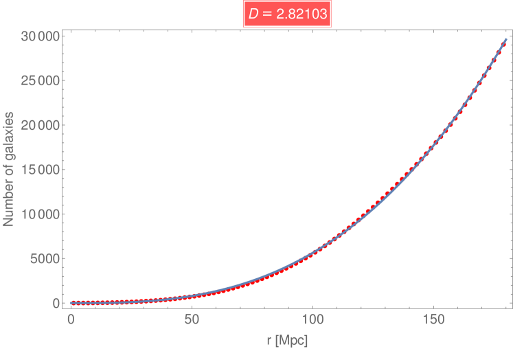
Figure 1: Mean number of galaxies reached by the growing spheres vs the radius of the spheres. One hundred galaxies were used as centers of the growing spheres. Dots are obtained from the computation, and solid red line indicates a fit of the form $ar^{D}$. From the fit, the obtained dimension is shown in the red box.

Table 1: Parameters of the fit plotted in Fig. 1, including the standard error and the t-statistic.

Parameter	​​​​Estimate	​​​​Standard Error	​​​​t-Statistic​​​​
$a$	0.013	0.00044	29.45
$D$	2.82103	0.00673	419.176

Fig. 2 shows the dimension $D$ as a function of the radius $r$. The decay of the dimension at large scales is due to boundary effects of the dataset. A dimension of $D=2$ in the scales of $[20,30]\leavevmode\nobreak\ \mathrm{Mpc}$ transitions and reaches $D=3$ at the scales $[60,70]\leavevmode\nobreak\ \mathrm{Mpc}$.

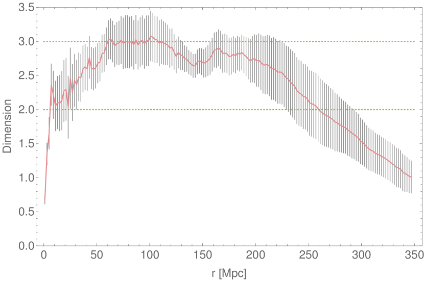
Figure 2: Dimension vs. radius. Dimension is plotted along with gray error bars. Dashed lines indicate dimensions 2 and 3.

In our second method, after building a graph using the galaxies as explained in Sec. 2, we can estimate the dimension of the graph counting the number of nodes that fall within a sphere of increasing radius and whose limit is the boundary of the graph. We can see this process in a qualitative way in in Fig. 3. In Fig. 4 we can see the estimation of the dimension starting for a single point in the graph, in this case the center and using a fit of the form $ar^{D}$ whose adjustment parameters can be found in the in Table 2. In Fig. 5 we show the dimension estimation using a graph of 51 845 nodes and considering 20 central nodes. We use several central nodes because the result may depend on certain central node $X$, then we average the counting using 20 central nodes. The error bars indicate $1\sigma$ ranges in the distribution of values obtained from different central nodes $X$.

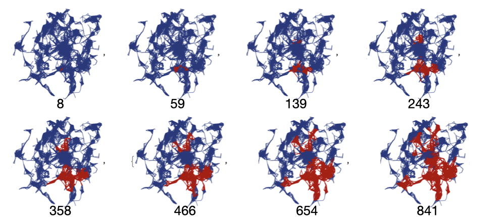
Figure 3: A representative graph using 1853 nodes. Starting from a central node $X$ in the graph, we count the number of nodes in the graph that can be reached by going out at most a distance $r$. In red color we can observe this process starting from the center of the graph. The number indicated below each graph is the total number of nodes counted up to a distance $r$.

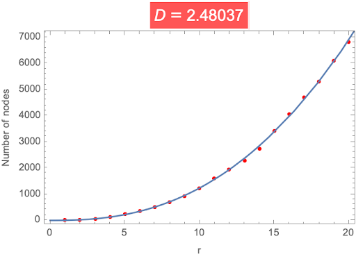
Figure 4: Estimation of the dimension starting for a unique position in the graph.

Table 2: Parameters of the fit plotted in Fig. 4, including the standard error and the t-statistic.

Parameter	​​​​Estimate	​​​​Standard Error	​​​​t-Statistic​​​​
$a$	4.098	0.256	15.974
$D$	2.48037	0.0219	113.182

4 Conclusions

• Using the two methods, either the integral correlation or the graph approximation, a fractal dimension is found before the transition to homogeneity.

• Using the first approach, a transition from $D=2$ to $D=3$ starts in the interval $[20,30]\leavevmode\nobreak\ \mathrm{Mpc}$ and ends in the interval $[60,70]\leavevmode\nobreak\ \mathrm{Mpc}$. Other works report a transition to homogeneity at larger scales, as Ntelis et al. (2017), Scrimgeour et al. (2012).

• Using the graph approach we found a region where the dimension of the graph is around $D=3$, and a region where the graph dimension is less than three, as seen with the first method.

• We add evidence about the non-homogeneity of the distribution of galaxies at certain scales. Finding a transition from $D=2$, corresponding to a distribution of galaxies where the matter is uniformly distributed on spherical surfaces surrounding the observation point, to $D=3$ corresponding to a homogeneous and isotropic distribution of galaxies.

4.1 Future Work

• Calculate the dimension of galaxy distribution using different methods.

• Use recent astronomical catalogs to consider more galaxies in the computations.

• Study the implications of fractality in the dynamics of galaxies using general relativity.

• Apply the methods used in this work to star formation regions, and compare with previous results as in Canavesi & Hurtado (2020).

• Analyze the implications of assuming a fractal gravitational model in astronomical and cosmological scales, as in Canavesi (2020).

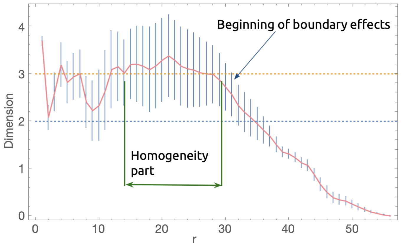
Figure 5: Dimension estimation as a function of the distance $r$ from the central nodes $X$. The graph has 51 845 nodes and several central nodes $X$ are used. The error bars indicate $1\sigma$ ranges in the distribution of values obtained from different central nodes $X$.

Thanks to the Wolfram Physics Project team for providing us with all the necessary software tools.

References

- Bagla et al. (2008) Bagla J.S., Yadav J., Seshadri T., 2008, Monthly Notices of the Royal Astronomical Society, 390, 829
- Canavesi (2020) Canavesi T., 2020, Boletin de la Asociacion Argentina de Astronomia La Plata Argentina, 61B, 136
- Canavesi & Hurtado (2020) Canavesi T., Hurtado S., 2020, Boletin de la Asociacion Argentina de Astronomia La Plata Argentina, 61B, 254
- Chacón & Casas (2009) Chacón C., Casas R., 2009, MOMENTO, 77–94
- Chacón-Cardona et al. (2016) Chacón-Cardona C., Casas-Miranda R., Muñoz-Cuartas J., 2016, Chaos, Solitons & Fractals, 82, 22
- (6) Inc. W.R., , Mathematica, Version 12.1. Champaign, IL, 2020
- Kamer et al. (2013) Kamer Y., Ouillon G., Sornette D., 2013, Physical Review E, 88, 022922
- Ntelis et al. (2017) Ntelis P., et al., 2017, Journal of Cosmology and Astroparticle Physics, 2017, 019
- Scrimgeour et al. (2012) Scrimgeour M.I., et al., 2012, Monthly Notices of the Royal Astronomical Society, 425, 116
- Wolfram (2020) Wolfram S., 2020, Complex Systems, 29(2), 107–536