BORE: Bayesian Optimization by Density-Ratio Estimation

Abstract

Bayesian optimization (bo) is among the most effective and widely-used blackbox optimization methods. bo proposes solutions according to an explore-exploit trade-off criterion encoded in an acquisition function, many of which are computed from the posterior predictive of a probabilistic surrogate model. Prevalent among these is the expected improvement (ei). The need to ensure analytical tractability of the predictive often poses limitations that can hinder the efficiency and applicability of bo. In this paper, we cast the computation of ei as a binary classification problem, building on the link between class-probability estimation and density-ratio estimation, and the lesser-known link between density-ratios and ei. By circumventing the tractability constraints, this reformulation provides numerous advantages, not least in terms of expressiveness, versatility, and scalability. author=C. Archambeau,color=gray!100!green!33,size=,]This needs to be more tangible. We need to quantify (give at least an example) the benefit! author=L. Tiao,color=blue!100!green!33,size=,]I need to emphasize that EI is usually expressed analytically as a combination of the properties of the posterior predictive, which is a major cause of the limitations–the need to ensure analytical tractability. And then I can explain that the increased flexibility and greater representational capacity comes from the alternate parameterization of EI as an arbitrarily powerful blackbox classifier, uninhibited by tractability constraints. Further, I need to say all this in one or two short sentences… author=C. Archambeau,color=gray!100!green!33,size=,]We claim that the tractability constraints are circumvented. This is great, but raises the question why this imatters given that EI is not considered the SotA acquisition function. We need to make clear that EI is (is it?) now more competitive with other acquisition functions. author=L. Tiao,color=blue!100!green!33,size=,]If we claim that EI, formulated in the way we do, makes it more competitive against other acquisition functions, we need to run comparisons with a fairly large set of them—or at the very least, UCB, ES, and PES. Until we actually do this, I’d rather just say something cliche like: “although EI is not the SOTA acquisition function, it is a practical, conceptually simple and effective choice that has withstood the test of time.” author=C. Archambeau,color=gray!100!green!33,size=,]It would have been sufficient to run against one, let say PES or MES. We may actually do that after submission to prepare for the rebuttal :-)

toltxlabel

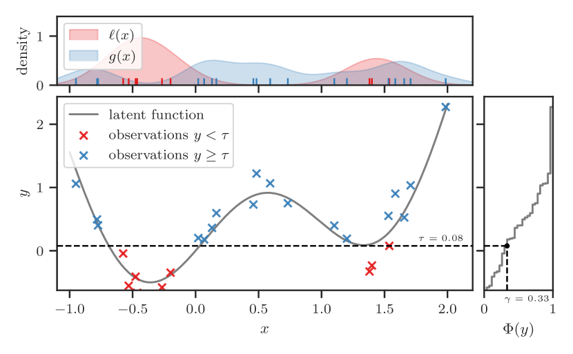
Figure 1: Optimizing a synthetic function $f(x)=\sin(3x)+x^{2}-0.7x$ with observation noise $\varepsilon\sim\mathcal{N}(0,0.2^{2})$. In the main pane, the noise-free function is represented by the solid gray curve, and $N=27$ noisy observations are represented by the crosses ‘$\times$’. Observations with output $y$ in the top performing $\gamma=\nicefrac{{1}}{{3}}$ proportion are shown in red; otherwise, they are shown in blue. Their corresponding densities, $\ell(x)$ and $g(x)$, respectively, are shown in the top pane. bore exploits the correspondence between the ei acquisition function and the ratio of densities $\nicefrac{{\ell(x)}}{{g(x)}}$.

author=C. Archambeau,color=gray!100!green!33,size=,]The last sentence is not informative and could confuse the reader. author=L. Tiao,color=blue!100!green!33,size=,]True, but the reader need look no further than Equation 5 to get the specifics; the teaser hopefully entices the reader to do that.

1 Introduction

Bayesian optimization (bo) is a sample-efficient methodology for the optimization of expensive blackbox functions (Brochu et al., 2010; Shahriari et al., 2015). In brief, bo proposes candidate solutions according to an acquisition function that encodes the explore-exploit trade-off. At the core of bo is a probabilistic surrogate model based on which the acquisition function can be computed.

Of the numerous acquisition functions that have been devised, the expected improvement (ei) (Mockus et al., 1978; Jones et al., 1998) remains predominant, due in large to its effectiveness in spite of its relative simplicity. In particular, while acquisition functions are generally difficult to compute, let alone optimize (Wilson et al., 2018), ei has a closed-form expression when the model’s posterior predictive is Gaussian. However, while this condition makes ei easier to work with, it can also preclude the use of richer families of models: one must ensure analytical tractability of the predictive, often at the expense of expressiveness, or otherwise resort to sampling-based approximations.

For instance, by virtue of its flexibility and well-calibrated predictive uncertainty (not to mention conjugacy properties), Gaussian process (gp) regression (Williams & Rasmussen, 1996) is a widely-used probabilistic model in bo. To extend gp-based bo to functions with discrete variables (Garrido-Merchán & Hernández-Lobato, 2020), structures with conditional dependencies (Jenatton et al., 2017), or to capture nonstationary phenomenon (Snoek et al., 2014), it is common to apply simple modifications to the covariance function, as this can often be done without compromising the tractability of the predictive. Suffice it to say, there exists estimators more naturally adept at dealing with these conditions (e.g. decision trees in the case of discrete variables). Indeed, to scale bo to problem settings that yield large numbers of observations, such as in transfer learning (Swersky et al., 2013), existing works have resorted to different families of models, such as random forests (rfs) (Hutter et al., 2011) and Bayesian neural networks (bnns) (Snoek et al., 2015; Springenberg et al., 2016; Perrone et al., 2018). However, these are either subject to constraints and simplifying assumptions, or must resort to Monte Carlo (mc) methods that make ei more cumbersome to evaluate and optimize.

author=L. Tiao,color=blue!100!green!33,size=,]This is true and a good point, but I don’t think we can claim that BORE does any better in this regard (it’s a mystery how exploration actually factors into this density-ratio formulation of EI) On the other hand, with BORE we can deploy models without worrying about making sure the posterior predictive is Gaussian. This is the point I really want to make with regard to NNs and RFs in BO. author=C. Archambeau,color=gray!100!green!33,size=,]You might want to cite https://arxiv.org/abs/1706.04599 author=L. Tiao,color=blue!100!green!33,size=,]This reference is more about calibration of deterministic neural network classifiers and less about predictive uncertainty of Bayesian neural networks(?)

Recognizing that the surrogate model is only a means to an end—namely, of formulating an acquisition function, we turn the spotlight away from the model and toward the acquisition function itself. To this end, we seek an alternative formulation of ei, specifically, one that potentially opens the door to more powerful estimators for which the predictive would otherwise be unwieldy or simply intractable to compute. author=C. Archambeau,color=gray!100!green!33,size=,]The wording is inaccurate. Even is the predictive posterior is analytically tractable, this does not mean the acquisition function is, nor that it is easy to evaluate. You might also have a predictive that is analytically tractable, but result in an acquisition function that can be easily evaluated. What you want to say is that we seek to express the acquisition function in an alternate form that does not impose constraints on the surrogate model author=L. Tiao,color=blue!100!green!33,size=,]What you say applies to acquisition functions _beyond_PI, EI and UCB, right? I am guessing you have ES, PES and max-value ES in mind? I think I just need to refer specifically to EI, rather than making claims about acquisition functions in general for which counterexamples and caveats abound. In particular, Bergstra et al. (2011) demonstrate that, remarkably, the ei function can be expressed as the relative ratio between two densities (Yamada et al., 2011). To estimate this ratio, they propose a method known as the tree-structured Parzen estimator (tpe), which naturally handles discrete and tree-structured inputs, and scales linearly with the number of observations. In spite of its many advantages, however, tpe is not without deficiencies.

This paper makes the following contributions. (i) In § 2 we revisit the tpe approach from first principles and identify its shortcomings for tackling the general density-ratio estimation (dre) problem. (ii) In § 3 we propose a simple yet powerful alternative that casts the computation of ei as probabilistic classification. This approach is built on the aforementioned link between ei and the relative density-ratio, and the correspondence between dre and class-probability estimation (cpe). As such, it retains the strengths of the tpe method while ameliorating many of its weaknesses. Perhaps most significantly, it enables one to leverage virtually any state-of-the-art classification method available. author=C. Archambeau,color=gray!100!green!33,size=,]I just commented out the above; too verbose and little added value. author=L. Tiao,color=blue!100!green!33,size=,]I will leave it out for now then, but I feel we do need to circle back to how this better addresses the limitations of GP-based BO: namely mixed continuous and discrete inputs, non-stationarities, heteroscedasticity and so on. Otherwise there is no point in spelling those out in the earlier paragraph. In  § 4 we discuss how our work relates to the existing state-of-the-art methods for blackbox optimization and demonstrate, through comprehensive experiments in § 5, that our approach competes well with these methods on a diverse range of problems. author=C. Archambeau,color=gray!100!green!33,size=,]Again you need to be more concrete about the benefits/gains!

2 Background

author=C. Archambeau,color=gray!100!green!33,size=,]You should restructure the Background section. My suggestion would be: 2.1 BO with EI; 2.2 Relation between EI and density ratio; 2.3 TPE. The density ratio paragraph could be integrated into 2.2 and pitfalls in 2.3.

Given a blackbox function $f:\mathcal{X}\to\mathbb{R}$, the goal of bo is to find an input ${\boldsymbol{\mathbf{x}}}\in\mathcal{X}$ at which it is minimized, given a set of $N$ input-output observations $\mathcal{D}_{N}=\{({\boldsymbol{\mathbf{x}}}_{n},y_{n})\}_{n=1}^{N}$, where output $y_{n}=f({\boldsymbol{\mathbf{x}}}_{n})+\varepsilon$ is assumed to be observed with noise $\varepsilon\sim\mathcal{N}(0,\sigma^{2})$. In particular, having specified a probabilistic surrogate model $\mathcal{M}$, its posterior predictive $p(y\,|\,{\boldsymbol{\mathbf{x}}},\mathcal{D}_{N})$ is used to compute the acquisition function $\alpha({\boldsymbol{\mathbf{x}}};\mathcal{D}_{N})$, a criterion that encapsulates the explore-exploit trade-off. Accordingly, candidate solutions are obtained by maximizing this criterion, ${\boldsymbol{\mathbf{x}}}_{N+1}=\operatorname*{arg\,max}_{{\boldsymbol{\mathbf{x}}}\in\mathcal{X}}\alpha({\boldsymbol{\mathbf{x}}};\mathcal{D}_{N})$. We now focus our discussion on the expected improvement (ei) function.

2.1 Expected improvement (EI)

We first specify a utility function that quantifies the nonnegative amount by which  $y$ improves upon some threshold $\tau$, $U({\boldsymbol{\mathbf{x}}},y,\tau)\coloneqq\max(\tau-y,0)$. Then, the ei function (Mockus et al., 1978) author=C. Archambeau,color=gray!100!green!33,size=,]I would simplify and get rid of $\Phi$ if possible; you can always use $p(y<\tau)$. Why using $I$ for utility and not $U$? Most importantly, the notion of improvement has not been introduced; you need to explain why you call $\max(\tau-y,0)$ improvement. author=L. Tiao,color=blue!100!green!33,size=,]“The improvement is the amount by which $y$ decreases over $\tau$” I feel spelling out what improvement means is both more verbose and less precise than the exact expression $\tau-y$, which we already provide. is defined as the expected value of $U({\boldsymbol{\mathbf{x}}},y,\tau)$ over the predictive

$$\alpha({\boldsymbol{\mathbf{x}}};\mathcal{D}_{N},\tau)\coloneqq\mathbb{E}_{p(y\,|\,{\boldsymbol{\mathbf{x}}},\mathcal{D}_{N})}[U({\boldsymbol{\mathbf{x}}},y,\tau)].$$ (1)

By convention, $\tau$ is set to the incumbent, or the lowest function value so far observed $\tau=\min_{n}y_{n}$ (Wilson et al., 2018). Suppose the predictive takes the form of a Gaussian,

$$p(y\,|\,{\boldsymbol{\mathbf{x}}},\mathcal{D}_{N})=\mathcal{N}(y\,|\,\mu({\boldsymbol{\mathbf{x}}}),\sigma^{2}({\boldsymbol{\mathbf{x}}})).$$ (2)

This leads to

$$\alpha({\boldsymbol{\mathbf{x}}};\mathcal{D}_{N},\tau)=\sigma({\boldsymbol{\mathbf{x}}})\cdot\left[\nu({\boldsymbol{\mathbf{x}}})\cdot\Psi(\nu({\boldsymbol{\mathbf{x}}}))+\psi(\nu({\boldsymbol{\mathbf{x}}}))\right],$$ (3)

where $\nu({\boldsymbol{\mathbf{x}}})\coloneqq\frac{\tau-\mu({\boldsymbol{\mathbf{x}}})}{\sigma({\boldsymbol{\mathbf{x}}})}$, and $\Psi,\psi$ denote the cdf and pdf of the normal distribution, respectively. While this exact expression is both easy to evaluate and optimize, the conditions necessary to satisfy Equation 2 can often come at the expense of flexibility and expressiveness. Instead, let us consider a fundamentally different way to express ei itself.

author=C. Archambeau,color=gray!100!green!33,size=,]In what sense is this a relaxation? author=L. Tiao,color=blue!100!green!33,size=,]Rather than defining the incumbent $\tau$ as the very best value observed so far, it is “relaxed” to be the $\gamma$-th percentile of the observed values for some $\gamma>0$. author=C. Archambeau,color=gray!100!green!33,size=,]You need to say that the goal is to maximize EI. You might want to repeat the exploit explore trade-off and say that the conventional setting makes an implicit choice. Different choices can be made changing the threshold. You could also cite this paper by James Wilson, et al.: Maximizing acquisition functions for Bayesian optimization.

2.2 Relative density-ratio

Let $\ell({\boldsymbol{\mathbf{x}}})$ and $g({\boldsymbol{\mathbf{x}}})$ be a pair of densities. The $\gamma$-relative density-ratio of $\ell({\boldsymbol{\mathbf{x}}})$ and $g({\boldsymbol{\mathbf{x}}})$ is defined as

$$r_{\gamma}({\boldsymbol{\mathbf{x}}})\coloneqq\frac{\ell({\boldsymbol{\mathbf{x}}})}{\gamma\ell({\boldsymbol{\mathbf{x}}})+(1-\gamma)g({\boldsymbol{\mathbf{x}}})},$$ (4)

where $\gamma\ell({\boldsymbol{\mathbf{x}}})+(1-\gamma)g({\boldsymbol{\mathbf{x}}})$ denotes the $\gamma$-mixture density with mixing proportion $0\leq\gamma<1$ (Yamada et al., 2011). Note that for $\gamma=0$, we recover the ordinary density-ratio $r_{0}({\boldsymbol{\mathbf{x}}})=\nicefrac{{\ell({\boldsymbol{\mathbf{x}}})}}{{g({\boldsymbol{\mathbf{x}}})}}$. Further, observe that $r_{\gamma}({\boldsymbol{\mathbf{x}}})=h_{\gamma}(r_{0}({\boldsymbol{\mathbf{x}}}))$ where $h_{\gamma}:u\mapsto\left(\gamma+u^{-1}(1-\gamma)\right)^{-1}$ for $u>0$. author=C. Archambeau,color=gray!100!green!33,size=,]The use of $\gamma$ is confusion; why would this correspond to quantiles of $y$? Btw you might want to say that $u$ is non-negative.

We now discuss the conditions under which ei can be expressed as the ratio in Equation 4. First, set the threshold $\tau$ as the $\gamma$-th quantile of the observed $y$ values, $\tau\coloneqq\Phi^{-1}(\gamma)$ where $\gamma=\Phi(\tau)\coloneqq p(y\leq\tau)$. author=L. Tiao,color=blue!100!green!33,size=,]We’ve dropped the conditioning on $\mathcal{D}_{N}$ here. Maybe mention this. Thereafter, define the pair of densities as $\ell({\boldsymbol{\mathbf{x}}})\coloneqq p\left({\boldsymbol{\mathbf{x}}}\,|\,y\leq\tau;\mathcal{D}_{N}\right)$ and $g({\boldsymbol{\mathbf{x}}})\coloneqq p\left({\boldsymbol{\mathbf{x}}}\,|\,y>\tau;\mathcal{D}_{N}\right)$. An illustrated example is shown in Figure 1. Under these conditions, Bergstra et al. (2011) demonstrate that the ei function can be expressed as the relative density-ratio, up to some constant factor

$$\alpha\left({\boldsymbol{\mathbf{x}}};\mathcal{D}_{N},\Phi^{-1}(\gamma)\right)\propto r_{\gamma}({\boldsymbol{\mathbf{x}}}).$$ (5)

For completeness, we provide a self-contained derivation in Appendix A. Thus, this reduces the problem of maximizing ei to that of maximizing the relative density-ratio,

$${\boldsymbol{\mathbf{x}}}_{N+1} =\operatorname*{arg\,max}_{{\boldsymbol{\mathbf{x}}}\in\mathcal{X}}\alpha\left({\boldsymbol{\mathbf{x}}};\mathcal{D}_{N},\Phi^{-1}(\gamma)\right)$$

$$=\operatorname*{arg\,max}_{{\boldsymbol{\mathbf{x}}}\in\mathcal{X}}r_{\gamma}({\boldsymbol{\mathbf{x}}}).$$ (6)

To estimate the unknown relative density-ratio, one can appeal to a wide variety of approaches from the dre literature (Sugiyama et al., 2012). We refer to this strategy as Bayesian optimization by density-ratio estimation (bore).

2.3 Tree-structured Parzen estimator

The tree-structured Parzen estimator (tpe) (Bergstra et al., 2011) is an instance of the bore framework that seeks to solve the optimization problem of Equation 6 by taking the following approach:

1. Since $r_{\gamma}({\boldsymbol{\mathbf{x}}})=h_{\gamma}(r_{0}({\boldsymbol{\mathbf{x}}}))$ where $h_{\gamma}$ is strictly non-decreasing, focus instead on maximizing $r_{0}({\boldsymbol{\mathbf{x}}})$,

   $${\boldsymbol{\mathbf{x}}}_{\star}=\operatorname*{arg\,max}_{{\boldsymbol{\mathbf{x}}}\in\mathcal{X}}r_{0}({\boldsymbol{\mathbf{x}}}).$$

   author=C. Archambeau,color=gray!100!green!33,size=,]Need to say non-decreasing as function of what. author=L. Tiao,color=blue!100!green!33,size=,]This would become a little verbose; I think it is obvious from the context.

2. Estimate the ordinary density-ratio $r_{0}({\boldsymbol{\mathbf{x}}})$ by separately estimating its constituent numerator $\ell({\boldsymbol{\mathbf{x}}})$ and denominator $g({\boldsymbol{\mathbf{x}}})$, using a tree-based variant of kernel density estimation (kde) (Silverman, 1986). author=C. Archambeau,color=gray!100!green!33,size=,]Did you define KDE? Perhaps you could indicate what tree-based refers to?

It is not hard to see why tpe might be favorable compared to methods based on gp regression—one now incurs an $\mathcal{O}(N)$ computational cost as opposed to the $\mathcal{O}(N^{3})$ cost of gp posterior inference. Furthermore, it is equipped to deal with tree-structured, mixed continuous, ordered and unordered discrete inputs. In spite of its advantages, tpe is not without shortcomings.

2.4 Potential pitfalls

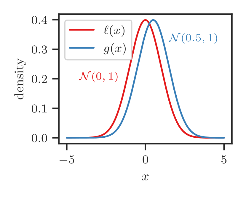
(a) Densities

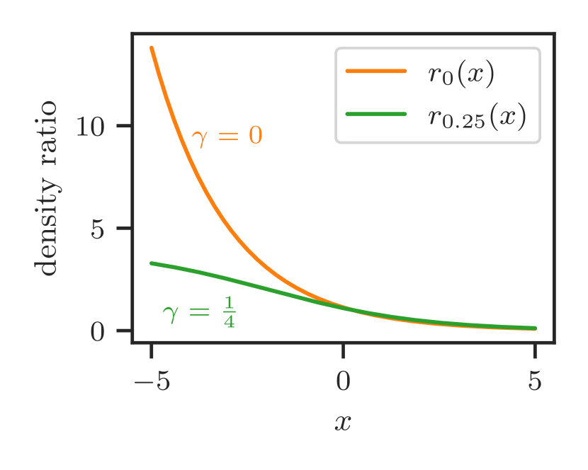
(b) Density-ratios

Figure 2: Gaussian densities and their $\gamma$-relative density-ratios, which diverges when $\gamma=0$ and converges to $4$ when $\gamma=\nicefrac{{1}}{{4}}$.

The shortcomings of this approach are already well-documented in the dre literature (Sugiyama et al., 2012). Nonetheless, we reiterate here a select few that are particularly detrimental in the context of global optimization. Namely, the first major drawback of tpe lies within Item 1:

Singularities. Relying on the ordinary density-ratio can result in numerical instabilities since it is unbounded—often diverging to infinity, even in simple toy scenarios (see Figure 2 for a simple example). In contrast, the $\gamma$-relative density-ratio is always bounded above by $\gamma^{-1}$ when $\gamma>0$ (Yamada et al., 2011). The other potential problems of tpe lie within Item 2:

Vapnik’s principle. Conceptually, independently estimating the densities is actually a more cumbersome approach that violates Vapnik’s principle—namely, that when solving a problem of interest, one should refrain from resorting to solve a more general problem as an intermediate step (Vapnik, 2013). In this instance, density estimation is a more general problem that is arguably more difficult than density-ratio estimation (Kanamori et al., 2010).

Kernel bandwidth. kde depends crucially on the selection of an appropriate kernel bandwidth, which is notoriously difficult (Park & Marron, 1990; Sheather & Jones, 1991). Furthermore, even with an optimal selection of a single fixed bandwidth, it cannot simultaneously adapt to low- and high-density regions (Terrell & Scott, 1992).

Error sensitivity. These difficulties are exacerbated by the fact that one is required to select two bandwidths, whereby the optimal bandwidth for one individual density is not necessarily appropriate for estimating the density-ratio—indeed, it may even have deleterious effects. This also makes the approach unforgiving to misspecification of the respective estimators, particularly in that of the denominator $g({\boldsymbol{\mathbf{x}}})$, which has a disproportionately large influence on the resulting density-ratio.

Curse of dimensionality. For these reasons and more, kde often falls short in high-dimensional regimes. In contrast, direct dre methods have consistently been shown to scale better with dimensionality (Sugiyama et al., 2008).

Optimization. Ultimately, we care not only about estimating the density-ratio, but also optimizing it wrt to inputs for the purpose of candidate suggestion. Being nondifferentiable, the ratio of tpes is cumbersome to optimize.

3 Methodology

We propose different approach to bore—importantly, one that circumvents the issues of tpe—by seeking to directly estimate the unknown ratio $r_{\gamma}({\boldsymbol{\mathbf{x}}})$. There exists a multitude of direct dre methods (see § 4). Here, we focus on a conceptually simple and widely-used method based on class-probability estimation (cpe) (Qin, 1998; Cheng et al., 2004; Bickel et al., 2007; Sugiyama et al., 2012; Menon & Ong, 2016).

First, let $\pi({\boldsymbol{\mathbf{x}}})=p(z=1\,|\,{\boldsymbol{\mathbf{x}}})$ denote the class-posterior probability, where $z$ is the binary class label

$$z\coloneqq\begin{cases}1&\text{if }y\leq\tau,\\ 0&\text{if }y>\tau.\end{cases}$$

By definition, we have $\ell({\boldsymbol{\mathbf{x}}})=p({\boldsymbol{\mathbf{x}}}\,|\,z=1)$ and $g({\boldsymbol{\mathbf{x}}})=p({\boldsymbol{\mathbf{x}}}\,|\,z=0)$. author=L. Tiao,color=blue!100!green!33,size=,]Note we’ve dropped the conditioning on $\mathcal{D}_{N}$ here. We plug these into Equation 4 and apply Bayes’ rule, letting the $p({\boldsymbol{\mathbf{x}}})$ terms cancel each other out to give

$$\begin{split}&r_{\gamma}({\boldsymbol{\mathbf{x}}})=\left(\frac{p(z=1\,|\,{\boldsymbol{\mathbf{x}}})}{p(z=1)}\right)\\ &\times\left(\gamma\cdot\frac{p(z=1\,|\,{\boldsymbol{\mathbf{x}}})}{p(z=1)}+(1-\gamma)\cdot\frac{p(z=0\,|\,{\boldsymbol{\mathbf{x}}})}{p(z=0)}\right)^{-1}\end{split}$$ (7)

Since $p(z=1)=\gamma$ by definition, Equation 7 simplifies to

$$r_{\gamma}({\boldsymbol{\mathbf{x}}})=\gamma^{-1}\pi({\boldsymbol{\mathbf{x}}}).$$ (8)

Refer to Appendix C for derivations. Thus, Equation 8 establishes the link between the class-posterior probability and the relative density-ratio. In particular, the latter is equivalent to the former up to constant factor $\gamma^{-1}$.

Let us estimate the probability $\pi({\boldsymbol{\mathbf{x}}})$ using a probabilistic classifier—a function $\pi_{\boldsymbol{\mathbf{\theta}}}:\mathcal{X}\to[0,1]$ parameterized by ${\boldsymbol{\mathbf{\theta}}}$. To recover the true class-posterior probability, we minimize a proper scoring rule (Gneiting & Raftery, 2007), such as the log loss

$$\begin{split}\mathcal{L}({\boldsymbol{\mathbf{\theta}}})&\coloneqq-\frac{1}{N}\left(\sum_{n=1}^{N}z_{n}\log{\pi_{\boldsymbol{\mathbf{\theta}}}({\boldsymbol{\mathbf{x}}}_{n})}\right.\\ &\qquad\left.\vphantom{\sum_{n=1}^{N}}+(1-z_{n})\log{(1-\pi_{\boldsymbol{\mathbf{\theta}}}({\boldsymbol{\mathbf{x}}}_{n}))}\right).\end{split}$$ (9)

Thereafter, we approximate the relative density-ratio up to constant $\gamma$ through

$$\pi_{\boldsymbol{\mathbf{\theta}}}({\boldsymbol{\mathbf{x}}})\simeq\gamma\cdot r_{\gamma}({\boldsymbol{\mathbf{x}}}),$$ (10)

with equality at ${\boldsymbol{\mathbf{\theta}}}_{\star}=\operatorname*{arg\,min}_{{\boldsymbol{\mathbf{\theta}}}}\mathcal{L}({\boldsymbol{\mathbf{\theta}}})$. Refer to Appendix D for derivations. Hence, in the so-called bo loop (summarized in Algorithm 1), we alternately optimize (i) the classifier parameters ${\boldsymbol{\mathbf{\theta}}}$ wrt to the log loss (to improve the approximation of Equation 10; Algorithm 1), and (ii) the classifier input ${\boldsymbol{\mathbf{x}}}$ wrt to its output (to suggest the next candidate to evaluate; Algorithm 1). An animation of Algorithm 1 is provided in Appendix E. author=C. Archambeau,color=gray!100!green!33,size=,]We should explain this in more length, referring to the relevant equations and repeating that step one corresponds to updating the posterior and step two to maximize EI. author=L. Tiao,color=blue!100!green!33,size=,]I do this in the next paragraph author=C. Archambeau,color=gray!100!green!33,size=,]Btw it is not clear to me how you compute the expectations wrt to l(x) and g(x). We should say a few words on that too.

In traditional gp-based ei, Algorithm 1 typically consists of maximizing the ei function expressed in the form of Equation 3, while Algorithm 1 consists of optimizing the gp hyperparameters wrt the marginal likelihood. author=L. Tiao,color=blue!100!green!33,size=,]People might nitpick here and point out that it is also possible to sample from approximate posterior and other things that are besides the point… By analogy with our approach, the parameterized function $\pi_{\boldsymbol{\mathbf{\theta}}}({\boldsymbol{\mathbf{x}}})$ is itself an approximation to the ei function to be maximized directly, while the approximation is tightened through by optimizing the classifier parameters wrt the log loss.

In short, we have reduced the problem of computing ei to that of learning a probabilistic classifier, thereby unlocking a broad range of estimators beyond those so far used in bo. Importantly, this enables one to employ virtually any state-of-the-art classification method available, and to parameterize the classifier using arbitrarily expressive approximators that potentially have the capacity to deal with non-linear, non-stationary, and heteroscedastic phenomena frequently encountered in practice. author=L. Tiao,color=blue!100!green!33,size=,]This sentence is too long

Input: blackbox $f:\mathcal{X}\to\mathbb{R}$, proportion $\gamma\in(0,1)$, probabilistic classifier $\pi_{{\boldsymbol{\mathbf{\theta}}}}:\mathcal{X}\to[0,1]$.

1 while under budget do

2       $\tau\leftarrow\Phi^{-1}(\gamma)$

3        // compute $\gamma$-th quantile of $\{y_{n}\}_{n=1}^{N}$

4       $z_{n}\leftarrow\mathbb{I}[y_{n}\leq\tau]$ for $n=1,\dotsc,N$

5        // assign labels

6       $\tilde{\mathcal{D}}_{N}\leftarrow\{({\boldsymbol{\mathbf{x}}}_{n},z_{n})\}_{n=1}^{N}$

7        // construct auxiliary dataset

8       /* update classifier by optimizing parameters ${\boldsymbol{\mathbf{\theta}}}$ wrt log loss */

9       ${\boldsymbol{\mathbf{\theta}}}_{\star}\leftarrow\operatorname*{arg\,min}_{\boldsymbol{\mathbf{\theta}}}\mathcal{L}({\boldsymbol{\mathbf{\theta}}})$

10        // depends on $\tilde{\mathcal{D}}_{N}$, see Equation 9

11       /* suggest candidate by optimizing input ${\boldsymbol{\mathbf{x}}}$ wrt classifier */

12       ${\boldsymbol{\mathbf{x}}}_{N}\leftarrow\operatorname*{arg\,max}_{{\boldsymbol{\mathbf{x}}}\in\mathcal{X}}\pi_{{\boldsymbol{\mathbf{\theta}}}_{\star}}({\boldsymbol{\mathbf{x}}})$

13        // see Equation 10

14       $y_{N}\leftarrow f({\boldsymbol{\mathbf{x}}}_{N})$

15        // evaluate blackbox function

16       $\mathcal{D}_{N}\leftarrow\mathcal{D}_{N-1}\cup\{({\boldsymbol{\mathbf{x}}}_{N},y_{N})\}$

17        // update dataset

18       $N\leftarrow N+1$

19 end while

Algorithm 1 Bayesian optimization by density-ratio estimation (bore).

author=C. Archambeau,color=gray!100!green!33,size=,]One might wonder why we still call Bayesian optimization. author=L. Tiao,color=blue!100!green!33,size=,]Agreed—just as people refer to TPE as a BO method, which is the apparently the subject of much controversy.

3.1 Choice of proportion $\gamma$

The proportion $\gamma\in(0,1)$ influences the explore-exploit trade-off. Intuitively, a smaller setting of $\gamma$ encourages exploitation and leads to fewer modes and sharper peaks in the acquisition function. To see this, consider that there are by definition fewer candidate inputs ${\boldsymbol{\mathbf{x}}}$ for which its corresponding output $y$ can be expected to improve over the first quartile ($\gamma=\nicefrac{{1}}{{4}}$) of the observed output values than, say, the third quartile ($\gamma=\nicefrac{{3}}{{4}}$). That being said, given that the class balance rate is by definition $\gamma$, a value too close to $0$ may lead to instabilities in classifier learning. A potential strategy to combat this is to begin with a perfect balance ($\gamma=\nicefrac{{1}}{{2}}$) and then to decay $\gamma$ as optimization progresses. In this work, we keep $\gamma$ fixed throughout optimization. This, on the other hand, has the benefit of providing guarantees about how the classification task evolves over iterations. In particular, in each iteration, after having observed a new evaluation, we are guaranteed that the binary label of at most one existing instance can flip. This property exploited to make classifier learning of Algorithm 1 more efficient by adopting online learning techniques that avoid learning from scratch in each iteration. An extended discussion is included in Appendix F.

3.2 Choice of probabilistic classifier

author=L. Tiao,color=blue!100!green!33,size=,]Note sure if this best fits here, or in the next (experiments) section.

We examine a few variations of bore that differ in the choice of classifier and discuss their strengths and weaknesses across different global optimization problem settings.

Multi-layer perceptrons.  We propose bore-mlp, a variant based on multi-layer perceptrons (mlps). This choice is appealing not only for (i) its flexibility and universal approximation guarantees (Hornik et al., 1989) but because (ii) one can easily adopt stochastic gradient descent (sgd) methods to scale up its parameter learning (LeCun et al., 2012), and (iii) it is differentiable end-to-end, thus enabling the use of quasi-Newton methods such as l-bfgs (Liu & Nocedal, 1989) for candidate suggestion. Lastly, since sgd is online by nature, (iv) it is feasible to adapt weights from previous iterations instead of training from scratch. A notable weakness is that mlps can be over-parameterized and therefore considerably data-hungry. author=L. Tiao,color=blue!100!green!33,size=,]Another downside is that they are so-so for discrete spaces and conditional spaces (requires a lot more work, but can be done).

Tree-based ensembles.  We propose two further variants: bore-rf and bore-xgb, both based on ensembles of decision trees—namely, random forest (rf) (Breiman, 2001) and gradient-boosted trees (xgboost) (Chen & Guestrin, 2016), respectively. These variants are attractive since they inherit from decision trees the ability to (i) deal with discrete and conditional inputs by design, (ii) work well in high-dimensions, and (iii) are scalable and easily parallelizable. Further, (iv) online extensions of rfs (Saffari et al., 2009) may be applied to avoid training from scratch.

A caveat is that, since their response surfaces are discontinuous and nondifferentiable, decision trees are difficult to maximize. Therefore, we appeal to random search and evolutionary strategies for candidate suggestion. Further details and a comparison of various approaches is included in § G.1.

In theory, for the approximation of Equation 10 to be tight, the classifier is required to produce well-calibrated probabilities (Menon & Ong, 2016). A potential drawback of the bore-rf variant is that rfs are generally not trained by minimizing a proper scoring rule. As such, additional techniques may be necessary to improve calibration (Niculescu-Mizil & Caruana, 2005).

author=C. Archambeau,color=gray!100!green!33,size=,]There should be a discussion about the class unbalance as well as the choice of $\gamma$.

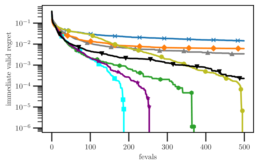
(a) protein

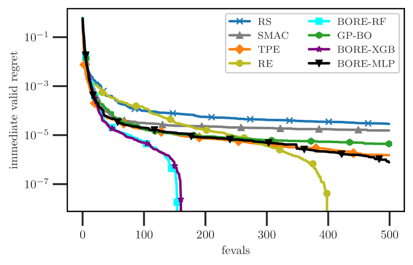
(b) naval

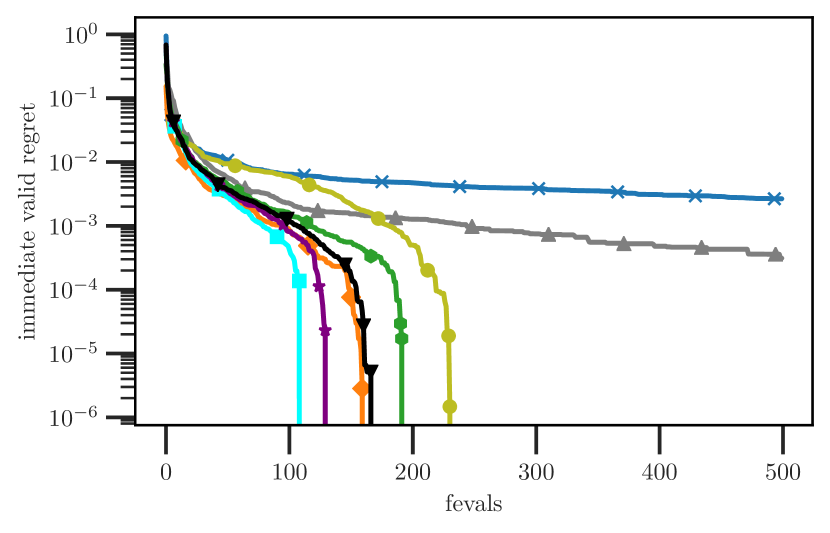
(c) parkinsons

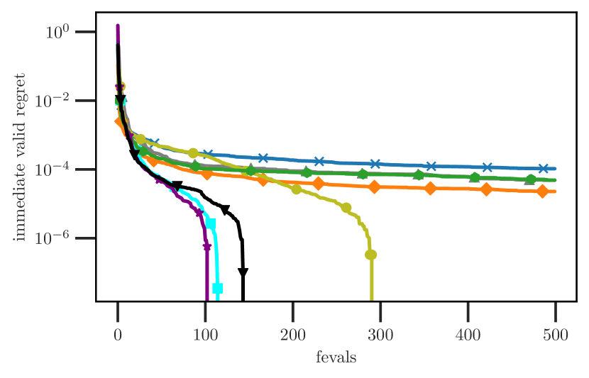
(d) slice

Figure 3: Immediate regret over function evaluations on the HPOBench neural network tuning problems ($D=9$).

4 Related Work

The literature on bo is vast and ever-expanding (Brochu et al., 2010; Shahriari et al., 2015; Frazier, 2018). Some specific threads pertinent to our work include achieving scalability through neural networks (nns), as in bananas (White et al., 2019), ablr (Perrone et al., 2018), bohamiann (Springenberg et al., 2016), and dngo (Snoek et al., 2015), and handling discrete and conditional variables using tree ensembles, as with rfs in smacs (Hutter et al., 2011). To negotiate the tractability of the predictive, these methods must either make simplifications or resort to approximations. In contrast, by seeking to directly approximate the acquisition function, bore is unencumbered by such constraints. Refer to § L.1 for an expanded discussion. author=L. Tiao,color=blue!100!green!33,size=,](Garrido-Merchán & Hernández-Lobato, 2020; Snoek et al., 2014) make patches to the kernel whereas we are free to adopt the class of estimators most appropriate to the problem at hand. mention this if we include in our comparisons Beyond the classical pi (Kushner, 1964) and ei functions (Jones et al., 1998), a multitude of acquisition functions have been devised, including the upper confidence bound (ucb) (Srinivas et al., 2009), knowledge gradient (kg) (Scott et al., 2011), entropy search (es) (Hennig & Schuler, 2012), and predictive es (pes) (Hernández-Lobato et al., 2014). author=L. Tiao,color=blue!100!green!33,size=,]The purpose of this paragraph is to (a) acknowledge that acquisition functions other than EI exist in BO, and (b) provide a justification for why one might still care to focus on EI with the existence of other, ostensibly better, options. Nonetheless, ei remains ubiquitous, in large because it is conceptually simple, easy to evaluate and optimize, and consistently performs well in practice.

There is a substantial body of existing works on density-ratio estimation (Sugiyama et al., 2012). Recognizing the deficiencies of the kde approach, a myriad alternatives have since been proposed, including kl importance estimation procedure (kliep) (Sugiyama et al., 2008), kernel mean matching (kmm) (Gretton et al., 2009), unconstrained least-squares importance fitting (ulsif) (Kanamori et al., 2009), and relative ulsif (rulsif) (Yamada et al., 2011). In this work, we restrict our focus on cpe, an effective and versatile approach that has found widespread adoption in a diverse range of applications, e.g. in covariate shift adaptation (Bickel et al., 2007), energy-based modelling (Gutmann & Hyvärinen, 2012), generative adversarial networks (gans) (Goodfellow et al., 2014; Nowozin et al., 2016), likelihood-free inference (Tran et al., 2017; Thomas et al., 2020), and more. Of particular relevance is its use in Bayesian experimental design (bed), a close relative of bo, wherein it is similarly applied to approximate the expected utility function (Kleinegesse & Gutmann, 2019). author=L. Tiao,color=blue!100!green!33,size=,]I use up all this space to enumerate these other applications to justify the reason we adopt the CPE and not any of the others aforementioned. But perhaps this is a bit much.

5 Experiments

We describe the experiments conducted to empirically evaluate our method. To this end, we consider a variety of problems, ranging from automated machine learning (automl), robotic arm control, to racing line optimization.

We provide comparisons against a comprehensive selection of state-of-the-art baselines. Namely, across all problems, we consider: random search (rs) (Bergstra & Bengio, 2012), gp-bo with ei, $\gamma=0$ (Jones et al., 1998), tpe (Bergstra et al., 2011), and smac (Hutter et al., 2011). We also consider evolutionary strategies: differential evolution (de) (Storn & Price, 1997) for problems with continuous domains, and regularized evolution (re) (Real et al., 2019) for those with discrete domains. Further information about these baselines and the source code for their implementations are included in Appendix I.

To quantitatively assess performance (on benchmarks for which the exact global minimum is known), we report the immediate regret, defined as the absolute error between the global minimum and the lowest function value attained thus far. Unless otherwise stated we report, for each benchmark and method, results aggregated across 100 replicated runs.

We set $\gamma=\nicefrac{{1}}{{3}}$ across all variants and benchmarks. For candidate suggestion in the tree-based variants, we use rs with a function evaluation limit of 500 for problems with discrete domains, and de with a limit of 2,000 for those with continuous domains. Further details concerning the experimental set-up and the implementation of each bore variant are included in Appendix J.

Neural network tuning (HPOBench).  First we consider the problem of training a two-layer feed-forward nn for regression. Specifically, a nn is trained for 100 epochs with the adam optimizer (Kingma & Ba, 2014), and the objective is the validation mean-squared error (mse). The hyperparameters are the initial learning rate, learning rate schedule, batch size, along with the layer-specific widths, activations and dropout rates. author=L. Tiao,color=blue!100!green!33,size=,]Should emphasize that all inputs are discrete ordered and unordered We consider four datasets: protein, naval, parkinsons and slice, and utilize HPOBench (Klein & Hutter, 2019) which tabulates, for each dataset, the mses resulting from all possible (62,208) configurations. Additional details are included in § K.1, and the results are shown in Figure 3. We see across all datasets that the bore-rf and -xgb variants consistently outperform all other baselines, converging rapidly toward the global minimum after 1-2 hundred evaluations—in some cases, earlier than any other baseline by over two hundred evaluations. Notably, with the exception being bore-mlp on the parkinsons dataset, all bore variants outperform tpe, in many cases by a sizable margin.

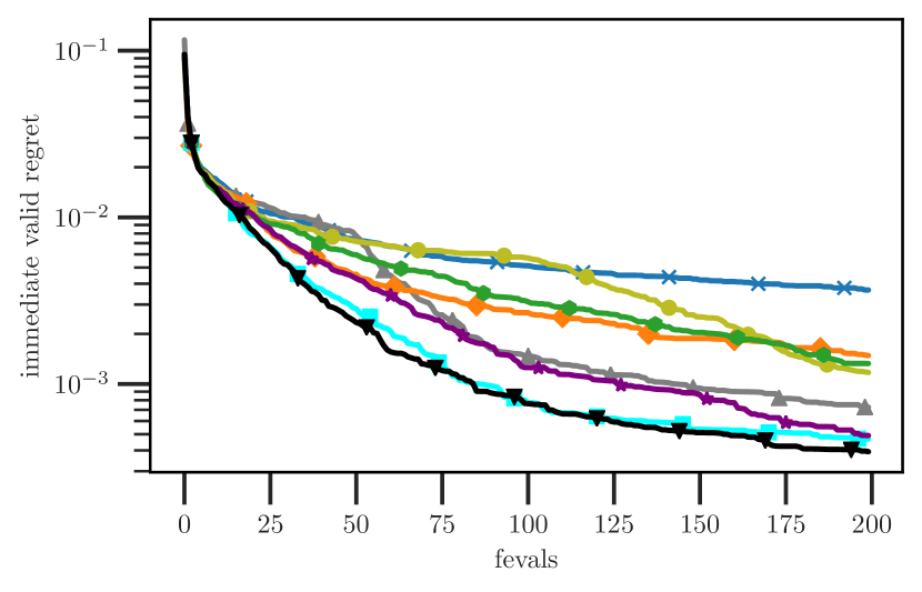
(a) CIFAR-10

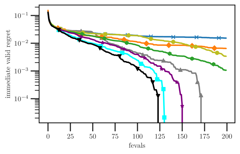
(b) CIFAR-100

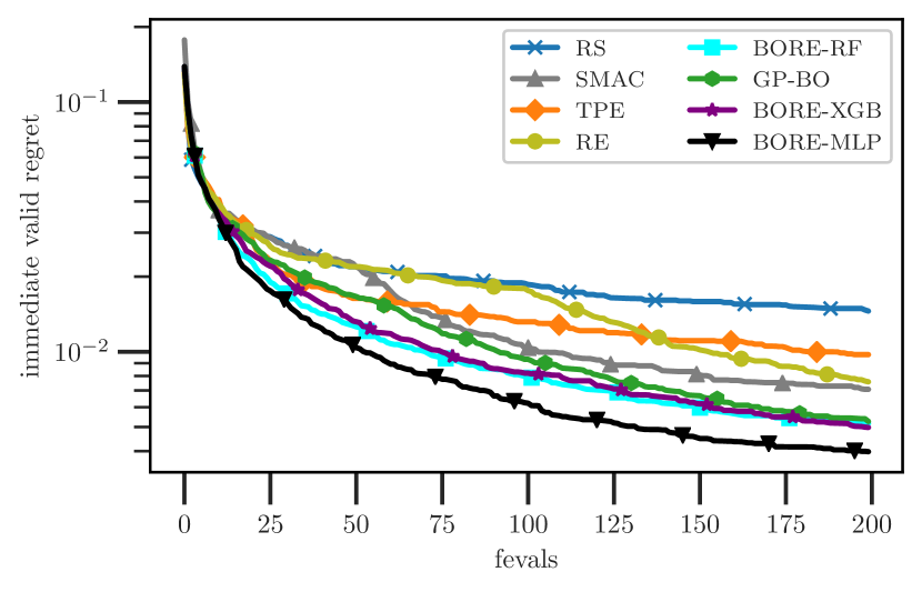
(c) ImageNet-16

Figure 4: Immediate regret over function evaluations on the NASBench201 neural architecture search problems ($D=6$).

Neural architecture search (NASBench201).  Next, we consider a neural architecture search (nas) problem, namely, that of designing a neural cell. A cell is represented by a directed acyclic graph (dag) with 4 nodes, and the task is to assign an operation to each of the 6 possible arcs from a set of five operations. author=L. Tiao,color=blue!100!green!33,size=,]If space becomes a problem: make this more concise or less specific; defer details to appendix We utilize NASBench201 (Dong & Yang, 2020), which tabulates precomputed results from all possible $5^{6}=15,625$ combinations for each of the three datasets: CIFAR-10, CIFAR-100 (Krizhevsky et al., 2009) and ImageNet-16 (Chrabaszcz et al., 2017). Additional details are included in § K.2, and the results are shown in Figure 4. We find across all datasets that the bore variants consistently achieve the lowest final regret among all baselines. Not only that, the bore variants, in particular bore-mlp, maintains the lowest regret at anytime (i.e. at any optimization iteration), followed by bore-rf, then bore-xgb. In this problem, the inputs are purely categorical, whereas in the previous problem they are a mix of categorical and ordinal. For the bore-mlp variant, categorical inputs are one-hot encoded, while ordinal inputs are handled by simply rounding to its nearest integer index. The latter is known to have shortcomings (Garrido-Merchán & Hernández-Lobato, 2020), and might explain why bore-mlp is the most effective variant in this problem but the least effective in the previous one.

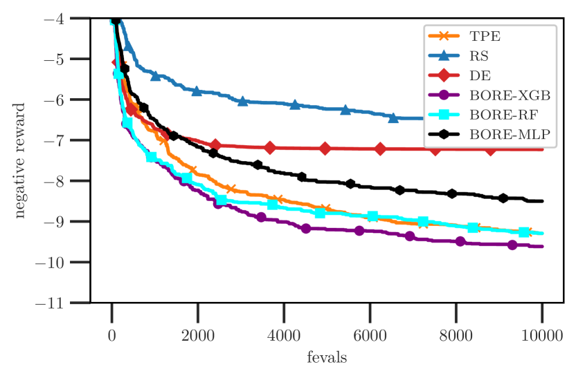
Figure 5: Negative reward over function evaluations on the Robot Pushing task ($D=14$).

Robot arm pushing.  We consider the 14D control problem first studied by Wang & Jegelka (2017). The problem is concerned with tuning the controllers of robot hands to push objects to some desired locations. Specifically, there are two robots, each tasked with manipulating an object. For each robot, the control parameters include the location and orientation of its hands, the moving direction, pushing speed, and duration. Due to the large number of function evaluations ($\sim$10,000) required to achieve a reasonable performance, we omit gp-bo from our comparisons on this benchmark. Further, we reduce the number of replicated runs of each method to 50. Additional details are included in § K.3, and the results are shown in Figure 5. We see that bore-xgb attains the highest reward, followed by bore-rf and tpe (which attain roughly the same performance), and then bore-mlp.

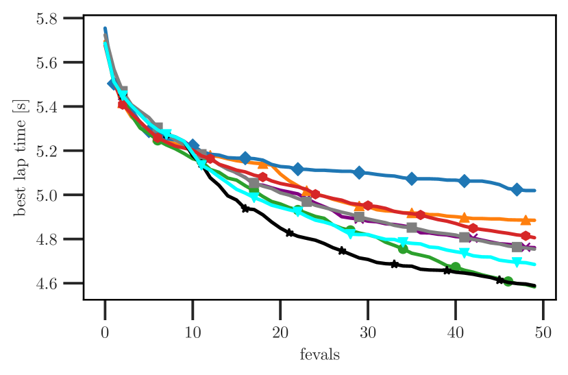
(a) uc berkeley ($D=12$)

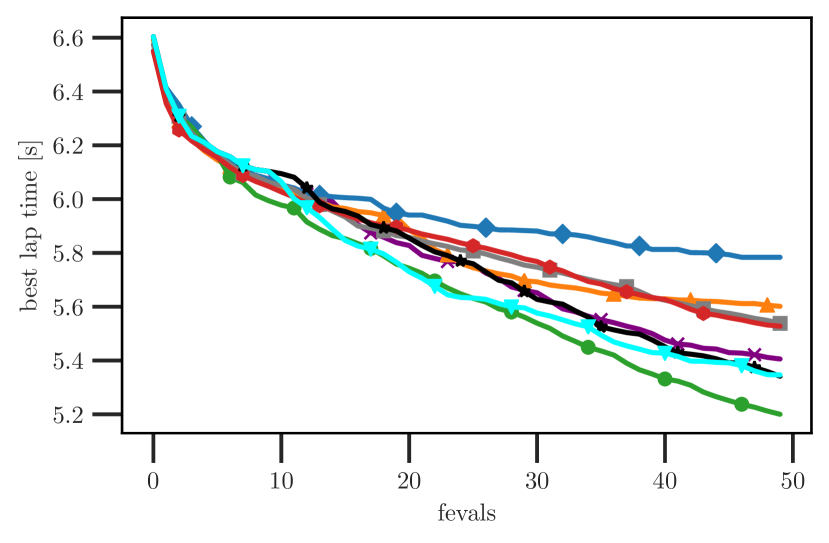
(b) eth zürich A ($D=20$)

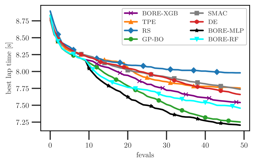
(c) eth zürich B ($D=21$)

Figure 6: Best lap times (in seconds) over function evaluations in the racing line optimization problem on various racetracks.

Racing line optimization.  We consider the problem of computing the optimal racing line for a given track and vehicle with known dynamics. We adopt the set-up of Jain & Morari (2020), who consider the dynamics of miniature scale cars traversing around tracks at uc berkeley and eth zürich. The racing line is a trajectory determined by $D$ waypoints placed along the length of the track, where the $i$th waypoint deviates from the centerline of the track by $x_{i}\in\left[-\frac{W}{2},\frac{W}{2}\right]$ for some track width $W$. The task is to minimize the lap time $f({\boldsymbol{\mathbf{x}}})$, the minimum time required to traverse the trajectory parameterized by ${\boldsymbol{\mathbf{x}}}=[x_{1}\cdots x_{D}]^{\top}$. Additional details are included in § K.4, and the results are shown in Figure 6. First, we see that the bore variants consistently outperform all baselines except for gp-bo. This is to be expected, since the function is continuous, smooth and has $\sim$20 dimensions or less. Nonetheless, we find that the bore-mlp variant performs as well as, or marginally better than, gp-bo on two tracks. In particular, on the uc berkeley track, we see that bore-mlp achieves the best lap times for the first $\sim$40 evaluations, and is caught up to by gp-bo in the final 10. On eth zürich track b, bore-mlp consistently maintains a narrow lead.

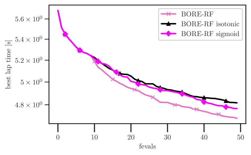
Figure 7: Effects of calibrating rfs in the bore-rf variant. Results of racing line optimization on the uc berkeley track.

Effects of calibration. As discussed in § 3.2, calibrating rfs may have a profound effect on the bore-rf variant. We consider two popular approaches (Niculescu-Mizil & Caruana, 2005), namely, Platt scaling (Platt et al., 1999) and isotonic regression (Zadrozny & Elkan, 2001, 2002). The results shown in Figure 7 suggest that applying these calibration techniques may have deleterious effects. However, this can also be adequately explained by overfitting due to insufficient calibration samples (in the case of isotonic regression, $\sim$1,000 samples are necessary). Therefore, we may yet observe the benefits of calibration in problem settings that yield large amounts of data.

We provide further ablation studies in Appendix G.

6 Discussion and Outlook

We examine the limitations of our method, discuss how these may be addressed, and outline additional future directions.

We restricted our attention to a simple treatment of hyperparameters ${\boldsymbol{\mathbf{\theta}}}$ based on point estimates. For example, in the bore-mlp variant this consists of the weights and biases. For improved exploration, it may be beneficial to consider placing a prior on ${\boldsymbol{\mathbf{\theta}}}$ and marginalizing out its uncertainty (Snoek et al., 2012). Refer to § L.2 for an expanded discussion. Further, compared against gp-bo, a potential downside of bore is that there may be vastly more meta-hyperparameters settings from which to choose. Whereas in gp-bo these might consist of, e.g. the choice of kernel and its isotropy, there are potentially many more possibilities in bore. In the case of bore-mlp, this may consist of, e.g. layer depth, widths, activations, etc—the tuning of which is often the reason one appeals to bo in the first place. While we obtained remarkable results with the proposed variants without needing to deviate from the sensible defaults, generally speaking, for further improvements in calibration and sample diversity, it may be beneficial to consider hyper-deep ensembles (Wenzel et al., 2020). Refer to § L.3 for further discussion.

Another avenue to explore is the potential benefits of other direct dre methods, in particular rulsif (Yamada et al., 2011), which is the only method of those aforementioned in § 4 that directly estimates the relative density-ratio. Furthermore, since rulsif is parameterized by a sum of Gaussian kernels, it enables the use of well-established mode-finding approaches, such as the mean-shift algorithm (Comaniciu & Meer, 2002), for candidate suggestion. Along the same avenue, but in a different direction, one may also consider employing dre losses for classifier learning (Menon & Ong, 2016).

Lastly, a fertile ground for exploration is extending bore with classifier designs suitable for bo more sophisticated paradigms, such as in the multi-task (Swersky et al., 2013), multi-fidelity (Kandasamy et al., 2017), and multi-objective settings (Hernández-Lobato et al., 2016), in addition to architectures effective for bo of sequences (Moss et al., 2020) and by extension, molecular structures (Gómez-Bombarelli et al., 2018) and beyond.

7 Conclusion

We have presented a novel methodology for bo based on the observation that the problem of computing ei can be reduced to that of probabilistic classification. This observation is made through the well-known link between cpe and dre, and the lesser-known insight that ei can be expressed as a relative density-ratio between two unknown distributions.

We discussed important ways in which tpe, an early attempt to exploit the latter link, falls short. Further, we demonstrated that our cpe-based approach to bore, in particular, our variants based on the mlp, rf and xgboost classifiers, consistently outperform tpe, and compete well against the state-of-the-art derivative-free global optimization methods.

Overall, the simplicity and effectiveness of bore make it a promising approach for blackbox optimization, and its high degree of extensibility provides numerous exciting avenues for future work.

Appendix A Expected improvement

For completeness, we reproduce the derivations of Bergstra et al. (2011). Recall from Equation 1 that the expected improvement (ei) function is defined as the expectation of the improvement utility function $U({\boldsymbol{\mathbf{x}}},y,\tau)$ over the posterior predictive distribution $p(y\,|\,{\boldsymbol{\mathbf{x}}},\mathcal{D}_{N})$. Expanding this out, we have

$$\alpha({\boldsymbol{\mathbf{x}}};\mathcal{D}_{N},\tau)\coloneqq\mathbb{E}_{p(y\,|\,{\boldsymbol{\mathbf{x}}},\mathcal{D}_{N})}[U({\boldsymbol{\mathbf{x}}},y,\tau)] =\int_{-\infty}^{\infty}U({\boldsymbol{\mathbf{x}}},y,\tau)p(y\,|\,{\boldsymbol{\mathbf{x}}},\mathcal{D}_{N})\,\mathrm{d}y$$

$$=\int_{-\infty}^{\tau}(\tau-y)p(y\,|\,{\boldsymbol{\mathbf{x}}},\mathcal{D}_{N})\,\mathrm{d}y$$

$$=\frac{1}{p({\boldsymbol{\mathbf{x}}}\,|\,\mathcal{D}_{N})}\int_{-\infty}^{\tau}(\tau-y)p({\boldsymbol{\mathbf{x}}}\,|\,y,\mathcal{D}_{N})p(y\,|\,\mathcal{D}_{N})\,\mathrm{d}y,$$

where we have invoked Bayes’ rule in the final step above. Next, the denominator evaluates to

$$p({\boldsymbol{\mathbf{x}}}\,|\,\mathcal{D}_{N}) =\int_{-\infty}^{\infty}p({\boldsymbol{\mathbf{x}}}\,|\,y,\mathcal{D}_{N})p(y\,|\,\mathcal{D}_{N})\,\mathrm{d}y$$

$$=\ell({\boldsymbol{\mathbf{x}}})\int_{-\infty}^{\tau}p(y\,|\,\mathcal{D}_{N})\,\mathrm{d}y+g({\boldsymbol{\mathbf{x}}})\int_{\tau}^{\infty}p(y\,|\,\mathcal{D}_{N})\,\mathrm{d}y$$

$$=\gamma\ell({\boldsymbol{\mathbf{x}}})+(1-\gamma)g({\boldsymbol{\mathbf{x}}}),$$

since, by definition, $\gamma=\Phi(\tau)\coloneqq p(y\leq\tau\,|\,\mathcal{D}_{N})$. Finally, we evaluate the numerator,

$$\int_{-\infty}^{\tau}(\tau-y)p({\boldsymbol{\mathbf{x}}}\,|\,y,\mathcal{D}_{N})p(y\,|\,\mathcal{D}_{N})\,\mathrm{d}y =\ell({\boldsymbol{\mathbf{x}}})\int_{-\infty}^{\tau}(\tau-y)p(y\,|\,\mathcal{D}_{N})\,\mathrm{d}y$$

$$=\ell({\boldsymbol{\mathbf{x}}})\tau\int_{-\infty}^{\tau}p(y\,|\,\mathcal{D}_{N})\,\mathrm{d}y-\ell({\boldsymbol{\mathbf{x}}})\int_{-\infty}^{\tau}yp(y\,|\,\mathcal{D}_{N})\,\mathrm{d}y$$

$$=\gamma\tau\ell({\boldsymbol{\mathbf{x}}})-\ell({\boldsymbol{\mathbf{x}}})\int_{-\infty}^{\tau}yp(y\,|\,\mathcal{D}_{N})\,\mathrm{d}y$$

$$=K\cdot\ell({\boldsymbol{\mathbf{x}}}),$$

where

$$K=\gamma\tau-\int_{-\infty}^{\tau}yp(y\,|\,\mathcal{D}_{N})\,\mathrm{d}y.$$

Hence, this shows that the ei function is equivalent to the $\gamma$-relative density ratio (Yamada et al., 2011) up to a constant factor $K$,

$$\alpha({\boldsymbol{\mathbf{x}}};\mathcal{D}_{N},\tau) \propto\frac{\ell({\boldsymbol{\mathbf{x}}})}{\gamma\ell({\boldsymbol{\mathbf{x}}})+(1-\gamma)g({\boldsymbol{\mathbf{x}}})}$$

$$=\left(\gamma+\frac{g({\boldsymbol{\mathbf{x}}})}{\ell({\boldsymbol{\mathbf{x}}})}(1-\gamma)\right)^{-1}.$$

Appendix B Relative density-ratio: unabridged notation

In § 2, for notational simplicity, we had excluded the dependencies of $\ell,g$ and $r_{\gamma}$ on $\tau$. Let us now define these densities more explicitly as

$$\ell({\boldsymbol{\mathbf{x}}};\tau)\coloneqq p\left({\boldsymbol{\mathbf{x}}}\,|\,y\leq\tau,\mathcal{D}_{N}\right),\qquad\text{and}\qquad g({\boldsymbol{\mathbf{x}}};\tau)\coloneqq p\left({\boldsymbol{\mathbf{x}}}\,|\,y>\tau,\mathcal{D}_{N}\right),$$

and accordingly, the $\gamma$-relative density-ratio from Equation 4 as

$$r({\boldsymbol{\mathbf{x}}};\gamma,\tau)=\frac{\ell({\boldsymbol{\mathbf{x}}};\tau)}{\gamma\ell({\boldsymbol{\mathbf{x}}};\tau)+(1-\gamma)g({\boldsymbol{\mathbf{x}}};\tau)}.$$

Recall from Equation 5 that

$$\alpha\left({\boldsymbol{\mathbf{x}}};\mathcal{D}_{N},\Phi^{-1}({\color[rgb]{0,0.44,0.57}\gamma})\right)\propto r\left({\boldsymbol{\mathbf{x}}};{\color[rgb]{0,0.44,0.57}\gamma},\Phi^{-1}({\color[rgb]{0,0.44,0.57}\gamma})\right).$$ (11)

In Item 1, Bergstra et al. (2011) resort to optimizing $r({\boldsymbol{\mathbf{x}}};0,\Phi^{-1}(\gamma))$, which is justified by the fact that

$$r({\boldsymbol{\mathbf{x}}};{\color[rgb]{0,0.44,0.57}\gamma},\Phi^{-1}({\color[rgb]{0,0.44,0.57}\gamma}))=h_{{\color[rgb]{0,0.44,0.57}\gamma}}\left[r\left({\boldsymbol{\mathbf{x}}};{\color[rgb]{1,0.49,0}0},\Phi^{-1}({\color[rgb]{0,0.44,0.57}\gamma})\right)\right],$$

for strictly nondecreasing $h_{\gamma}$. Note we have used a blue and orange color coding to emphasize the differences in the setting of $\gamma$ (best viewed on a computer screen). Recall that $\Phi^{-1}(0)=\min_{n}y_{n}$ corresponds to the conventional setting of threshold $\tau$. However, make no mistake, for any $\gamma>0$,

$$\alpha\left({\boldsymbol{\mathbf{x}}};\mathcal{D}_{N},\Phi^{-1}({\color[rgb]{1,0.49,0}0})\right)\not\propto r\left({\boldsymbol{\mathbf{x}}};{\color[rgb]{1,0.49,0}0},\Phi^{-1}({\color[rgb]{0,0.44,0.57}\gamma})\right).$$

Therefore, given the numerical instabilities associated with this approach as discussed in § 2.4, there is no advantage to be gained from taking this direction. Moreover, Equation 11 only holds for $\gamma>0$. To see this, suppose $\gamma=0$, which gives

$$\alpha\left({\boldsymbol{\mathbf{x}}};\mathcal{D}_{N},\Phi^{-1}({\color[rgb]{0,0.44,0.57}0})\right)\propto r\left({\boldsymbol{\mathbf{x}}};{\color[rgb]{0,0.44,0.57}0},\Phi^{-1}({\color[rgb]{0,0.44,0.57}0})\right).$$

However, since by definition $\ell\left({\boldsymbol{\mathbf{x}}};\Phi^{-1}(0)\right)$ has no mass, the rhs is undefined.

Appendix C Class-posterior probability

We provide an unabridged derivation of the identity of Equation 8. First, the $\gamma$-relative density ratio is given by

$$r_{\gamma}({\boldsymbol{\mathbf{x}}}) \coloneqq\frac{\ell({\boldsymbol{\mathbf{x}}})}{\gamma\ell({\boldsymbol{\mathbf{x}}})+(1-\gamma)g({\boldsymbol{\mathbf{x}}})}$$

$$=\frac{p({\boldsymbol{\mathbf{x}}}\,|\,z=1)}{\gamma\cdot p({\boldsymbol{\mathbf{x}}}\,|\,z=1)+(1-\gamma)\cdot p({\boldsymbol{\mathbf{x}}}\,|\,z=0)}$$

$$=\left(\frac{p(z=1\,|\,{\boldsymbol{\mathbf{x}}})\cancel{p({\boldsymbol{\mathbf{x}}})}}{p(z=1)}\right)\left(\gamma\cdot\frac{p(z=1\,|\,{\boldsymbol{\mathbf{x}}})\cancel{p({\boldsymbol{\mathbf{x}}})}}{p(z=1)}+(1-\gamma)\cdot\frac{p(z=0\,|\,{\boldsymbol{\mathbf{x}}})\cancel{p({\boldsymbol{\mathbf{x}}})}}{p(z=0)}\right)^{-1}.$$

By construction, we have $p(z=1)\coloneqq p(y\leq\tau)=\gamma$ and $\pi({\boldsymbol{\mathbf{x}}})\coloneqq p(z=1\,|\,{\boldsymbol{\mathbf{x}}})$. Therefore,

$$r_{\gamma}({\boldsymbol{\mathbf{x}}}) =\gamma^{-1}\pi({\boldsymbol{\mathbf{x}}})\left(\cancel{\gamma}\cdot\frac{\pi({\boldsymbol{\mathbf{x}}})}{\cancel{\gamma}}+\cancel{(1-\gamma)}\cdot\frac{1-\pi({\boldsymbol{\mathbf{x}}})}{\cancel{1-\gamma}}\right)^{-1}$$

$$=\gamma^{-1}\pi({\boldsymbol{\mathbf{x}}}).$$

Alternatively, we can also arrive at the same result by writing the ordinary density ratio $r_{0}({\boldsymbol{\mathbf{x}}})$ in terms of $\pi({\boldsymbol{\mathbf{x}}})$ and $\gamma$, which is well-known to be

$$r_{0}({\boldsymbol{\mathbf{x}}})=\left(\frac{\gamma}{1-\gamma}\right)^{-1}\frac{\pi({\boldsymbol{\mathbf{x}}})}{1-\pi({\boldsymbol{\mathbf{x}}})}.$$

Plugging this into function $h_{\gamma}$, we get

$$r_{\gamma}({\boldsymbol{\mathbf{x}}})=h_{\gamma}(r_{0}({\boldsymbol{\mathbf{x}}})) =h_{\gamma}\left(\left(\frac{\gamma}{1-\gamma}\right)^{-1}\frac{\pi({\boldsymbol{\mathbf{x}}})}{1-\pi({\boldsymbol{\mathbf{x}}})}\right)$$

$$=\left(\gamma+(1-\gamma)\left(\frac{\gamma}{1-\gamma}\right)\left(\frac{\pi({\boldsymbol{\mathbf{x}}})}{1-\pi({\boldsymbol{\mathbf{x}}})}\right)^{-1}\right)^{-1}$$

$$=\gamma^{-1}\left(1+\left(\frac{\pi({\boldsymbol{\mathbf{x}}})}{1-\pi({\boldsymbol{\mathbf{x}}})}\right)^{-1}\right)^{-1}$$

$$=\gamma^{-1}\pi({\boldsymbol{\mathbf{x}}}).$$

Appendix D Log loss

The log loss, also known as the binary cross-entropy (bce) loss, is given by

$$\mathcal{L}^{*}({\boldsymbol{\mathbf{\theta}}})\coloneqq-\beta\cdot\mathbb{E}_{\ell({\boldsymbol{\mathbf{x}}})}[\log{\pi_{\boldsymbol{\mathbf{\theta}}}({\boldsymbol{\mathbf{x}}})}]-(1-\beta)\cdot\mathbb{E}_{g({\boldsymbol{\mathbf{x}}})}[\log{(1-\pi_{\boldsymbol{\mathbf{\theta}}}({\boldsymbol{\mathbf{x}}}))}],$$ (12)

where $\beta$ denotes the class balance rate. In particular, let $N_{\ell}$ and $N_{g}$ be the sizes of the support of $\ell({\boldsymbol{\mathbf{x}}})$ and $g({\boldsymbol{\mathbf{x}}})$, respectively. Then, we have

$$\beta=\frac{N_{\ell}}{N},\qquad\text{and}\qquad 1-\beta=\frac{N_{g}}{N},$$

where $N=N_{\ell}+N_{g}$. In practice, we approximate the log loss $\mathcal{L}^{*}({\boldsymbol{\mathbf{\theta}}})$ by the empirical risk of Equation 9, given by

$$\mathcal{L}({\boldsymbol{\mathbf{\theta}}})\coloneqq-\frac{1}{N}\left(\sum_{n=1}^{N}z_{n}\log{\pi_{\boldsymbol{\mathbf{\theta}}}({\boldsymbol{\mathbf{x}}}_{n})}+(1-z_{n})\log{(1-\pi_{\boldsymbol{\mathbf{\theta}}}({\boldsymbol{\mathbf{x}}}_{n}))}\right).$$

In this section, we show that the approximation of Equation 10, that is,

$$\pi_{\boldsymbol{\mathbf{\theta}}}({\boldsymbol{\mathbf{x}}})\simeq\gamma\cdot r_{\gamma}({\boldsymbol{\mathbf{x}}}),$$

attains equality at ${\boldsymbol{\mathbf{\theta}}}_{\star}=\operatorname*{arg\,min}_{{\boldsymbol{\mathbf{\theta}}}}\mathcal{L}^{*}({\boldsymbol{\mathbf{\theta}}})$.

D.1 Optimum

Taking the functional derivative of $\mathcal{L}^{*}$ in Equation 12, we get

$$\frac{\partial\mathcal{L}^{*}}{\partial\pi_{\boldsymbol{\mathbf{\theta}}}} =-\mathbb{E}_{\ell({\boldsymbol{\mathbf{x}}})}\left[\frac{\beta}{\pi_{\boldsymbol{\mathbf{\theta}}}({\boldsymbol{\mathbf{x}}})}\right]+\mathbb{E}_{g({\boldsymbol{\mathbf{x}}})}\left[\frac{1-\beta}{1-\pi_{\boldsymbol{\mathbf{\theta}}}({\boldsymbol{\mathbf{x}}})}\right]$$

$$=\int\left(-\beta\frac{\ell({\boldsymbol{\mathbf{x}}})}{\pi_{\boldsymbol{\mathbf{\theta}}}({\boldsymbol{\mathbf{x}}})}+(1-\beta)\frac{g({\boldsymbol{\mathbf{x}}})}{1-\pi_{\boldsymbol{\mathbf{\theta}}}({\boldsymbol{\mathbf{x}}})}\right)\mathrm{d}{\boldsymbol{\mathbf{x}}}$$

This integral evaluates to zero iff the integrand itself evaluates to zero. Hence, we solve the following for $\pi_{{\boldsymbol{\mathbf{\theta}}}_{\star}}({\boldsymbol{\mathbf{x}}})$,

$$\beta\frac{\ell({\boldsymbol{\mathbf{x}}})}{\pi_{{\boldsymbol{\mathbf{\theta}}}_{\star}}({\boldsymbol{\mathbf{x}}})}=(1-\beta)\frac{g({\boldsymbol{\mathbf{x}}})}{1-\pi_{{\boldsymbol{\mathbf{\theta}}}_{\star}}({\boldsymbol{\mathbf{x}}})}.$$

We re-arrange this expression to give

$$\frac{1-\pi_{{\boldsymbol{\mathbf{\theta}}}_{\star}}({\boldsymbol{\mathbf{x}}})}{\pi_{{\boldsymbol{\mathbf{\theta}}}_{\star}}({\boldsymbol{\mathbf{x}}})}=\left(\frac{1-\beta}{\beta}\right)\frac{g({\boldsymbol{\mathbf{x}}})}{\ell({\boldsymbol{\mathbf{x}}})}\qquad\Leftrightarrow\qquad\frac{1}{\pi_{{\boldsymbol{\mathbf{\theta}}}_{\star}}({\boldsymbol{\mathbf{x}}})}-1=\frac{\beta\ell({\boldsymbol{\mathbf{x}}})+(1-\beta)g({\boldsymbol{\mathbf{x}}})}{\beta\ell({\boldsymbol{\mathbf{x}}})}-1.$$

Finally, we add one to both sides and invert the result to give

$$\pi_{{\boldsymbol{\mathbf{\theta}}}_{\star}}({\boldsymbol{\mathbf{x}}}) =\frac{\beta\ell({\boldsymbol{\mathbf{x}}})}{\beta\ell({\boldsymbol{\mathbf{x}}})+(1-\beta)g({\boldsymbol{\mathbf{x}}})}$$

$$=\beta\cdot r_{\beta}({\boldsymbol{\mathbf{x}}}).$$

Since, by definition $\beta=\gamma$, this leads to $\pi_{{\boldsymbol{\mathbf{\theta}}}_{\star}}({\boldsymbol{\mathbf{x}}})=\gamma\cdot r_{\gamma}({\boldsymbol{\mathbf{x}}})$ as required.

D.2 Empirical risk minimization

For completeness, we show that the log loss $\mathcal{L}^{*}({\boldsymbol{\mathbf{\theta}}})$ of Equation 12 can be approximated by $\mathcal{L}({\boldsymbol{\mathbf{\theta}}})$ of Equation 9. First, let $\rho$ be the permutation of the set $\{1,\dotsc,N\}$, i.e. the bijection from $\{1,\dotsc,N\}$ to itself, such that $y_{\rho(n)}\leq\tau$ if $0<\rho(n)\leq N_{\ell}$, and $y_{\rho(n)}>\tau$ if $N_{\ell}<\rho(n)\leq N_{g}$. That is to say,

$${\boldsymbol{\mathbf{x}}}_{\rho(n)}\sim\begin{cases}\ell({\boldsymbol{\mathbf{x}}})&\text{if }0<\rho(n)\leq N_{\ell},\\ g({\boldsymbol{\mathbf{x}}})&\text{if }N_{\ell}<\rho(n)\leq N_{g}.\end{cases}\quad\text{and}\quad z_{\rho(n)}\coloneqq\begin{cases}1&\text{if }0<\rho(n)\leq N_{\ell},\\ 0&\text{if }N_{\ell}<\rho(n)\leq N_{g}.\end{cases}$$

Then, we have

$$\mathcal{L}^{*}({\boldsymbol{\mathbf{\theta}}}) \coloneqq-\frac{1}{N}\left(N_{\ell}\cdot\mathbb{E}_{\ell({\boldsymbol{\mathbf{x}}})}[\log{\pi_{\boldsymbol{\mathbf{\theta}}}({\boldsymbol{\mathbf{x}}})}]+N_{g}\cdot\mathbb{E}_{g({\boldsymbol{\mathbf{x}}})}[\log{(1-\pi_{\boldsymbol{\mathbf{\theta}}}({\boldsymbol{\mathbf{x}}}))}]\right)$$

$$\simeq-\frac{1}{N}\left(\cancel{N_{\ell}}\cdot\frac{1}{\cancel{N_{\ell}}}\sum_{n=1}^{N_{\ell}}\log{\pi_{\boldsymbol{\mathbf{\theta}}}({\boldsymbol{\mathbf{x}}}_{\rho(n)})}+\cancel{N_{g}}\cdot\frac{1}{\cancel{N_{g}}}\sum_{n=N_{\ell}+1}^{N_{g}}\log{(1-\pi_{\boldsymbol{\mathbf{\theta}}}({\boldsymbol{\mathbf{x}}}_{\rho(n)}))}\right)$$

$$=-\frac{1}{N}\left(\sum_{n=1}^{N}z_{\rho(n)}\log{\pi_{\boldsymbol{\mathbf{\theta}}}({\boldsymbol{\mathbf{x}}}_{\rho(n)})}+(1-z_{\rho(n)})\log{(1-\pi_{\boldsymbol{\mathbf{\theta}}}({\boldsymbol{\mathbf{x}}}_{\rho(n)}))}\right)$$

$$=-\frac{1}{N}\left(\sum_{n=1}^{N}z_{n}\log{\pi_{\boldsymbol{\mathbf{\theta}}}({\boldsymbol{\mathbf{x}}}_{n})}+(1-z_{n})\log{(1-\pi_{\boldsymbol{\mathbf{\theta}}}({\boldsymbol{\mathbf{x}}}_{n}))}\right)\coloneqq\mathcal{L}({\boldsymbol{\mathbf{\theta}}}),$$

as required.

Appendix E Step-through visualization

For illustration purposes, we go through Algorithm 1 step-by-step on a synthetic problem for a half-dozen iterations. Specifically, we minimize the forrester function

$$f(x)\coloneqq(6x-2)^{2}\sin{(12x-4)},$$

in the domain $x\in[0,1]$ with observation noise $\varepsilon\sim\mathcal{N}(0,0.05^{2})$. See Figure 8.

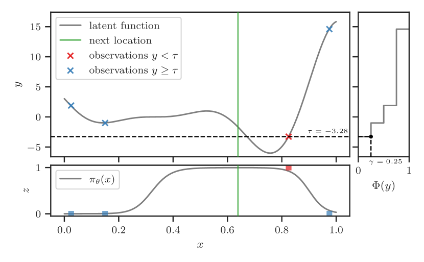
(a) Iteration 1

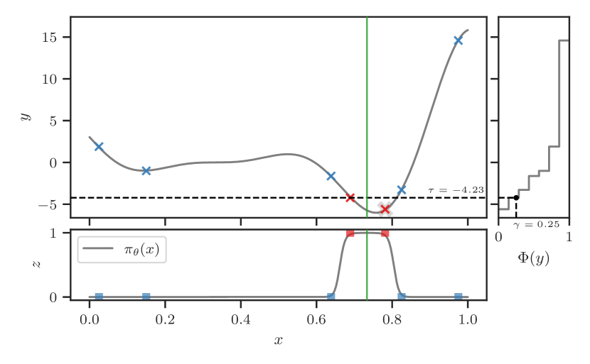
(b) Iteration 4

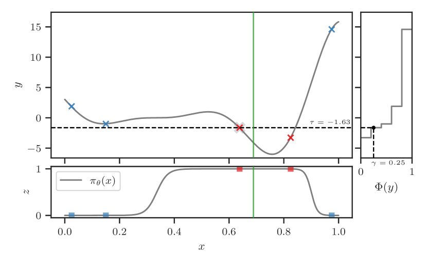
(c) Iteration 2

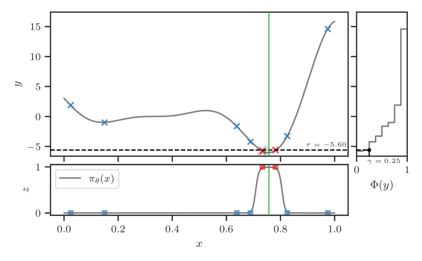
(d) Iteration 5

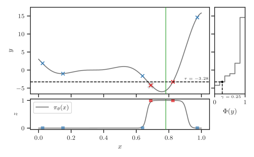
(e) Iteration 3

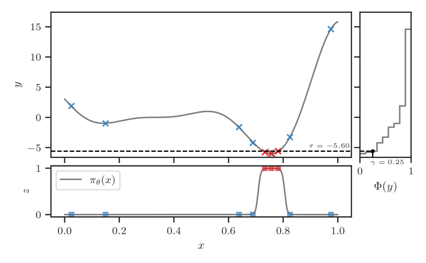
(f) Iteration 6

Figure 8: We go through Algorithm 1 step-by-step on a synthetic problem for a half-dozen iterations. Specifically, we minimize the forrester function. The algorithm is started 4 random initial designs. Each subfigure depicts the state after Algorithms 1 and 1—namely, after updating and maximizing the classifier. In every subfigure, the main pane depicts the noise-free function, represented by the solid gray curve, and the set of observations, represented by crosses ‘$\times$’. The location that was evaluated in the previous iteration is highlighted with a gray outline. The right pane shows the ecdf of the observed $y$ values. The vertical dashed black line in this pane is located at $\gamma=\frac{1}{4}$. The horizontal dashed black line is located at $\tau$, the value of $y$ such that $\Phi(y)=\frac{1}{4}$, i.e., $\tau=\Phi^{-1}\left(\frac{1}{4}\right)$. The instances below this horizontal line are assigned binary label $z=1$, while those above are assigned $z=0$. This is visualized in the bottom pane, alongside the probabilistic classifier $\pi_{\boldsymbol{\mathbf{\theta}}}({\boldsymbol{\mathbf{x}}})$, represented by the solid gray curve. Finally, the maximizer of the classifier is represented by the vertical solid green line—this denotes the location to be evaluated in the next iteration.

Appendix F Properties of the classification problem

We outline some notable properties of the bore classification problem as alluded to in § 3.

Class imbalance.  By construction, this problem has class balance rate $\gamma$.

Label changes across iterations.  Assuming the proportion $\gamma$ is fixed across iterations, then, in each iteration, we are guaranteed the following changes:

1. a new input and its corresponding output $({\boldsymbol{\mathbf{x}}}_{N},y_{N})$ will be added to the dataset, thus

2. creating a shift in the rankings and, by extension, quantiles of the observed $y$ values, in turn

3. leading to the binary label of at most one instance to flip.

Therefore, between consecutive iterations, changes to the classification dataset are fairly incremental. This property can be exploited to make classifier training more efficient, especially in families of classifiers for which re-training entirely from scratch in each iteration may be superfluous and wasteful. See Figure 9 for an illustrated example.

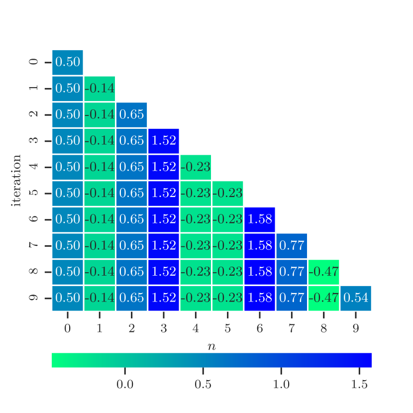
(a) Continuous targets $y_{n}$

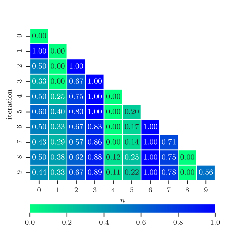
(b) Empirical distribution $\Phi(y_{n})$

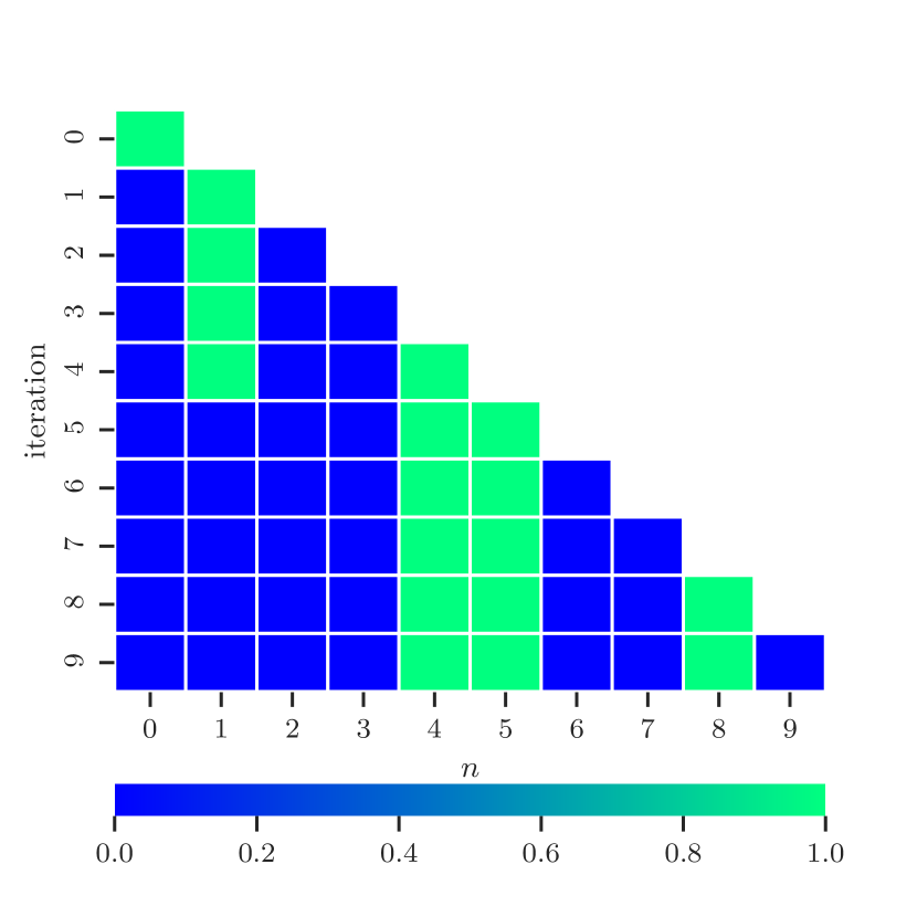
(c) Binary labels $z_{n}$

Figure 9: Optimizing a “noise-only” synthetic function $f(x)=0$ with observation noise $\varepsilon\sim\mathcal{N}(0,1)$. The proportion is set to $\gamma=\nicefrac{{1}}{{4}}$. As we iterate through the bo loop from top to bottom, the array of targets grows from left to right. Suffice it to say, in each iteration the size of the array increases by one, resulting in a re-shuffling of the rankings and, by extension, quantiles. This in turn leads to the label for at most one instance to flip. Hence, between consecutive iterations, changes to the classification dataset are fairly incremental. This property can be exploited to make classifier training more efficient in each iteration.

Some viable strategies for reducing per-iteration classier learning overhead may include speeding up convergence by (i) importance sampling (e.g. re-weighting new samples and those for which the label have flipped), (ii) early-stopping (stop training early if either the loss or accuracy have not changed for some number of epochs) and (iii) annealing (decaying the number of epochs or batch-wise training steps as optimization progresses).

Appendix G Ablation studies

G.1 Maximizing the acquisition function

We examine different strategies for maximizing the acquisition function (i.e. the classifier) in the tree-based variants of bore, namely, bore-rf and bore-xgb. Decision trees are difficult to maximize since their response surfaces are discontinuous and nondifferentiable. Hence, we consider the following methods: random search (rs) and differential evolution (de). For each method, we further consider different evaluation budgets, i.e. limits on the number of evaluations of the acquisition function. Specifically, we consider the limits $50,100,200,$ and $500$.

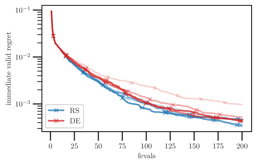
(a) bore-rf on CIFAR-10

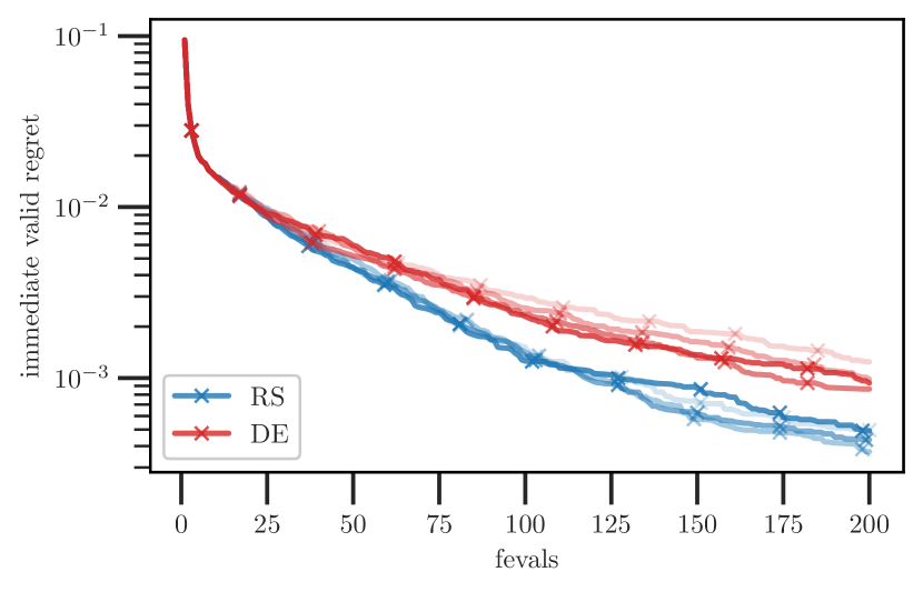
(b) bore-xgb on CIFAR-10

Figure 10: A comparison of various acquisition optimization strategies on the NASBench201 problem.

In Figures 10(a) and 10(b), we show the results of bore-rf and bore-xgb, respectively, on the CIFAR-10 dataset of the NASBench201 benchmark, as described in § K.2. Each curve represents the mean across 100 repeated runs. The opacity is proportional to the function evaluation limit, with the most transparent having the lowest limit and the most opaque having the highest limit. We find that rs appears to outperform de by a narrow margin. Additionally, for de, a higher evaluation limit appears to be somewhat beneficial, while the opposite holds for rs.

G.2 Effects of calibration

xgboost.  We apply the calibration approaches (Niculescu-Mizil & Caruana, 2005) we considered in § 5 to xgboost for the bore-xgb variant, namely, Platt scaling (Platt et al., 1999) and isotonic regression (Zadrozny & Elkan, 2001, 2002). As before, the results shown in Figure 11 seem to suggest that these calibration methods have deleterious effects—at least when considering optimization problems which require only a small number of function evaluations to reach the global minimum, since this yields a small dataset with which to calibrate the probabilistic classifier, making it susceptible to overfitting.

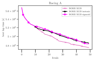
Figure 11: Effects of calibrating xgboost in the bore-xgb variant. Results of racing line optimization on the uc berkeley track.

Appendix H Toy example: relative density-ratio estimation by probabilistic classification

Consider the following toy example where the densities $\ell(x)$ and $g(x)$ are known and given exactly by the following (mixture of) Gaussians,

$$\ell(x)\coloneqq 0.3\mathcal{N}(2,1^{2})+0.7\mathcal{N}(-3,0.5^{2}),\qquad\text{and}\qquad g(x)\coloneqq\mathcal{N}(0,2^{2}),$$

as illustrated by the solid red and blue lines in Figure 12(a), respectively.

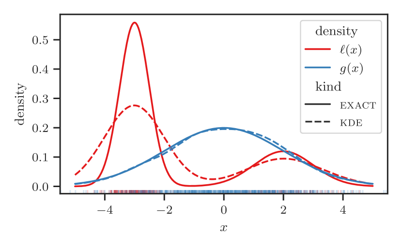
(a) Densities $\ell(x)$ and $g(x)$.

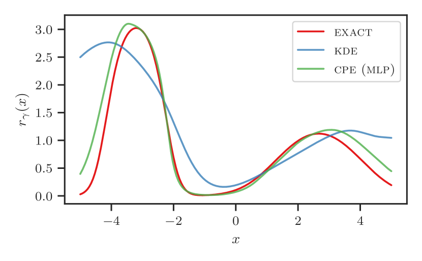
(b) Relative density-ratio, estimated with an mlp classifier.

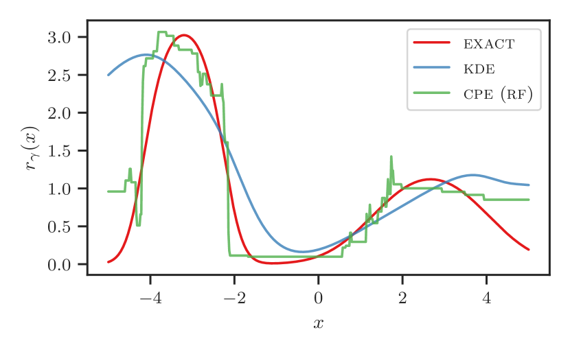
(c) Relative density-ratio, estimated with a rf classifier.

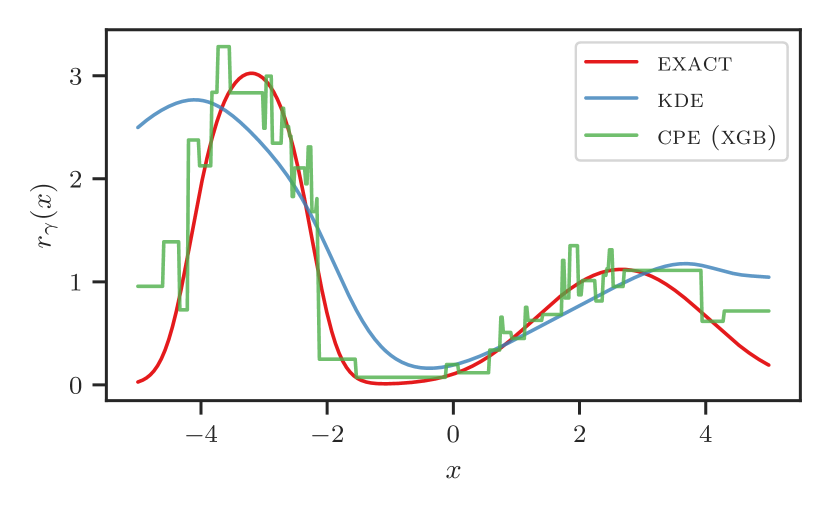
(d) Relative density-ratio, estimated with an xgboost classifier.

Figure 12: Synthetic toy example with (mixtures of) Gaussians.

We draw a total of $N=1000$ samples from these distributions, with a fraction $\gamma=\nicefrac{{1}}{{4}}$ drawn from $\ell(x)$ and the remainder from $g(x)$. These are represented by the vertical markers along the bottom of the $x$-axis (a so-called “rug plot”). Then, two kernel density estimations (kdes), shown with dashed lines, are fit on these respective sample sets, with kernel bandwidths selected according to the “normal reference” rule-of-thumbauthor=L. Tiao,color=blue!100!green!33,size=,]citation needed?. We see that, for both densities, the modes are recovered well, while for $\ell(x)$, the variances are overestimated in both of its mixture components. As we shall see, this has deleterious effects on the resulting density ratio estimate.

In Figure 12(b), we represent the true relative density-ratio with the red line. The estimate resulting from taking the ratio of the kdes is shown in blue, while that of the class-probability estimation (cpe) method described in § 3 is shown in green. In this subfigure, the probabilistic classifier consists of a simple multi-layer perceptron (mlp) with 3 hidden layers, each with and 32 units and $\mathtt{elu}$ activations. In Figures 12(c) and 12(d), we show the same, but with random forest (rf) and xgboost classifiers.

The cpe methods appear, at least visually, to recover the exact density ratios well, whereas the kde method does so quite poorly. Perhaps the more important quality to focus on, for the purposes of bo, is the mode of the density-ratio functions. In the case of the kde method, we can see that this deviates significantly from that of the true density-ratio. In this instance, even though kde fit $g(x)$ well and recovered the modes of $\ell(x)$ accurately, a slight overestimation of the variance in the latter led to a significant shift in the maximum of the resulting density-ratio functions.

Appendix I Implementation of Baselines

The software implementations of the baseline methods considered in our comparisons are described in Table 1.

Table 1: Implementations of baseline methods.

Method	Software Library	URL (github.com/*)	Notes
tpe	HyperOpt	hyperopt/hyperopt
smac	SMAC3	automl/SMAC3
gp-bo	AutoGluon	awslabs/autogluon	in autogluon.searcher.GPFIFOSearcher
de	-	-	custom implementation
re	NASBench-101	automl/nas_benchmarks	in experiment_scripts/run_regularized_evolution.py

Appendix J Experimental Set-up and Implementation Details

Hardware.  In our experiments, we employ m4.xlarge aws ec2 instances, which have the following specifications:

• CPU: Intel(R) Xeon(R) E5-2676 v3 (4 Cores) @ 2.4 GHz

• Memory: 16GiB (DDR3)

Software.  Our method is implemented as a configuration generator plug-in in the HpBandSter library of Falkner et al. (2018). The code will be released as open-source software upon publication.

The implementations of the classifiers on which the proposed variants of bore are based are described in Table 2.

Table 2: Implementations of classifiers.

Model	Software Library	URL
Multi-layer perceptron (mlp)	Keras	https://keras.io
Random forest (rf)	scikit-learn	https://scikit-learn.org
Gradient-boosted trees (xgboost)	XGBoost	https://xgboost.readthedocs.io

We set out with the aim of devising a practical method that is not only agnostic to the of choice classifier, but also robust to underlying implementation details—down to the choice of algorithmic settings. Ideally, any instantiation of bore should work well out-of-the-box without the need to tweak the sensible default settings that are typically provided by software libraries. Therefore, unless otherwise stated, we emphasize that made no effort was made to adjust any settings and all reported results were obtained using the defaults. For reproducibility, we explicitly enumerate them in turn for each of the proposed variants.

J.1 bore-rf

We limit our description to the most salient hyperparameters. We do not deviate from the default settings which, at the time of this writing, are:

• number of trees – 100

• minimum number of samples required to split an internal node (min_samples_split) – 2

• maximum depth – unspecified (nodes are expanded until all leaves contain less than min_samples_split samples)

J.2 bore-xgb

• number of trees (boosting rounds) – 100

• learning rate ($\eta$) – $0.3$

• minimum sum of instance weight (Hessian) needed in a child (min_child_weight) – 1

• maximum depth – 6

J.3 bore-mlp

In the bore-mlp variant, the classifier is a mlp with 2 hidden layers, each with 32 units. We consistently found $\mathtt{elu}$ activations (Clevert et al., 2015) to be particularly effective for lower-dimensional problems, with $\mathtt{relu}$ remaining otherwise the best choice. We optimize the weights with adam (Kingma & Ba, 2014) using batch size of $B=64$. For candidate suggestion, we optimize the input of the classifier wrt to its output using multi-started l-bfgs with three random restarts.

Epochs per iteration.  To ensure the training time on bo iteration $N$ is nonincreasing as a function of $N$, instead of directly specifying the number of epochs (i.e. full passes over the data), we specify the number of (batch-wise gradient) steps $S$ to train for in each iteration. Since the number of steps per epoch is $M=\lceil\nicefrac{{N}}{{B}}\rceil$, the effective number of epochs on the $N$-th bo iteration is then $E=\lfloor\nicefrac{{S}}{{M}}\rfloor$. For example, if $S=800$ and $B=64$, the number of epochs for iteration $N=512$ would be $E=100$. As another example, for all $0<N\leq B$ (i.e. we have yet to observe enough data to fill a batch), we have $E=S=800$. See Figure 13 for a plot of the effective number of epochs against iterations for different settings of batch size $B$ and number of steps per epoch $S$. Across all our experiments, we fix $S=100$.

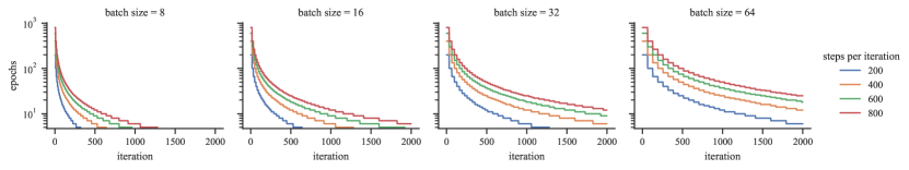
Figure 13: Effective number of epochs on the $n$th iteration for different settings of batch size $B$ and number of steps per epoch $S$.

Appendix K Details of Benchmarks

K.1 HPOBench

The hyperparameters for the HPOBench problem and their ranges are summarized in Table 3.

Table 3: Configuration space for HPOBench.

Hyperparameter		Range
Initial learning rate (lr)		$\{$5\text{\times}{10}^{-4}$,$1\text{\times}{10}^{-3}$,$5\text{\times}{10}^{-3}$,$1\text{\times}{10}^{-2}$,$5\text{\times}{10}^{-2}$,$1\text{\times}{10}^{-1}$\}$
lr schedule		$\{\mathtt{cosine},\mathtt{fixed}\}$
Batch size		$\{2^{3},2^{4},2^{5},2^{6}\}$
Layer 1	Width	$\{2^{4},2^{5},2^{6},2^{7},2^{8},2^{9}\}$
	Activation	$\{\mathtt{relu},\mathtt{tanh}\}$
	Dropout rate	$\{0.0,0.3,0.6\}$
Layer 2	Width	$\{2^{4},2^{5},2^{6},2^{7},2^{8},2^{9}\}$
	Activation	$\{\mathtt{relu},\mathtt{tanh}\}$
	Dropout rate	$\{0.0,0.3,0.6\}$

All hyperparameters are discrete—either ordered or unordered. All told, there are $6\times 2\times 4\times 6\times 2\times 3\times 6\times 2\times 3=66,208$ possible combinations. Further details on this problem can be found in (Klein & Hutter, 2019).

K.2 NASBench201

The hyperparameters for the HPOBench problem and their ranges are summarized in Table 4.

Table 4: Configuration space for NASBench-201.

Hyperparameter	Range
Arc 0	$\{\mathtt{none},\mathtt{skip}\text{-}\mathtt{connect},\mathtt{conv}\text{-}\mathtt{1\times 1},\mathtt{conv}\text{-}\mathtt{3\times 3},\mathtt{avg}\text{-}\mathtt{pool}\text{-}\mathtt{3\times 3}\}$
Arc 1	$\{\mathtt{none},\mathtt{skip}\text{-}\mathtt{connect},\mathtt{conv}\text{-}\mathtt{1\times 1},\mathtt{conv}\text{-}\mathtt{3\times 3},\mathtt{avg}\text{-}\mathtt{pool}\text{-}\mathtt{3\times 3}\}$
Arc 2	$\{\mathtt{none},\mathtt{skip}\text{-}\mathtt{connect},\mathtt{conv}\text{-}\mathtt{1\times 1},\mathtt{conv}\text{-}\mathtt{3\times 3},\mathtt{avg}\text{-}\mathtt{pool}\text{-}\mathtt{3\times 3}\}$
Arc 3	$\{\mathtt{none},\mathtt{skip}\text{-}\mathtt{connect},\mathtt{conv}\text{-}\mathtt{1\times 1},\mathtt{conv}\text{-}\mathtt{3\times 3},\mathtt{avg}\text{-}\mathtt{pool}\text{-}\mathtt{3\times 3}\}$
Arc 4	$\{\mathtt{none},\mathtt{skip}\text{-}\mathtt{connect},\mathtt{conv}\text{-}\mathtt{1\times 1},\mathtt{conv}\text{-}\mathtt{3\times 3},\mathtt{avg}\text{-}\mathtt{pool}\text{-}\mathtt{3\times 3}\}$
Arc 5	$\{\mathtt{none},\mathtt{skip}\text{-}\mathtt{connect},\mathtt{conv}\text{-}\mathtt{1\times 1},\mathtt{conv}\text{-}\mathtt{3\times 3},\mathtt{avg}\text{-}\mathtt{pool}\text{-}\mathtt{3\times 3}\}$

The operation associated with each of the $\binom{4}{2}=6$ arcs can belong to one of five categories. Hence, there are $5^{6}=15,625$ possible combinations of hyperparameter configurations. Further details on this problem can be found in (Dong & Yang, 2020).

K.3 Robot pushing control

This problem is concerned with tuning the controllers of two robot hands, with the goal of each pushing an object to some prescribed goal location ${\boldsymbol{\mathbf{p}}}_{g}^{(1)}$ and ${\boldsymbol{\mathbf{p}}}_{g}^{(2)}$, respectively. Let ${\boldsymbol{\mathbf{p}}}_{s}^{(1)}$ and ${\boldsymbol{\mathbf{p}}}_{s}^{(2)}$ denote the specified starting positions, and ${\boldsymbol{\mathbf{p}}}_{f}^{(1)}$ and ${\boldsymbol{\mathbf{p}}}_{f}^{(2)}$ the final positions (the latter of which are functions of the control parameters ${\boldsymbol{\mathbf{x}}}$). The reward is defined as

$$R({\boldsymbol{\mathbf{x}}})\coloneqq\underbrace{\|{\boldsymbol{\mathbf{p}}}_{g}^{(1)}-{\boldsymbol{\mathbf{p}}}_{s}^{(1)}\|+\|{\boldsymbol{\mathbf{p}}}_{g}^{(2)}-{\boldsymbol{\mathbf{p}}}_{s}^{(2)}\|}_{\text{initial distances}}-\underbrace{(\|{\boldsymbol{\mathbf{p}}}_{g}^{(1)}-{\boldsymbol{\mathbf{p}}}_{f}^{(1)}\|+\|{\boldsymbol{\mathbf{p}}}_{g}^{(2)}-{\boldsymbol{\mathbf{p}}}_{f}^{(2)}\|)}_{\text{final distances}},$$

which effectively quantifies the amount of progress made toward pushing the objects to the desired goal. For each robot, the control parameters include the location and orientation of its hands, the pushing speed, moving direction and push duration. These parameters and their ranges are summarized in Table 5.

Table 5: Configuration space for the robot pushing control problem.

Hyperparameter		Range
Robot 1	Position $x$	$[-5,5]$
	Position $y$	$[-5,5]$
	Angle $\theta$	$[0,2\pi]$
	Velocity $v_{x}$	$[-10,10]$
	Velocity $v_{y}$	$[-10,10]$
	Push Duration	$[2,30]$
	Torque	$[-5,5]$
Robot 2	Position $x$	$[-5,5]$
	Position $y$	$[-5,5]$
	Angle $\theta$	$[0,2\pi]$
	Velocity $v_{x}$	$[-10,10]$
	Velocity $v_{y}$	$[-10,10]$
	Push Duration	$[2,30]$
	Torque	$[-5,5]$

Further details on this problem can be found in (Wang et al., 2018). This simulation is implemented with the Box2D library, and the associated code repository can be found at https://github.com/zi-w/Ensemble-Bayesian-Optimization.

K.4 Racing line optimization

This problem is concerned with finding the optimal racing line. Namely, given a racetrack and a vehicle with known dynamics, the task is to determine a trajectory around the track for which the minimum time required to traverse it is minimal. We adopt the set-up of Jain & Morari (2020), who consider 1:10 and 1:43 scale miniature remote-controlled cars traversing tracks at UC Berkeley (Liniger et al., 2015) and ETH Zürich (Rosolia & Borrelli, 2019), respectively.

The trajectory is represented by a cubic spline parameterized by the 2D coordinates of $D$ waypoints, each placed at locations along the length of the track, where the $i$th waypoint deviates from the centerline of the track by $x_{i}\in\left[-\frac{W}{2},\frac{W}{2}\right]$, for some track width $W$. Hence, the parameters are the distances by which each waypoint deviates from the centerline, ${\boldsymbol{\mathbf{x}}}=[x_{1}\cdots x_{D}]^{\top}$.

Our blackbox function of interest, namely, the minimum time to traverse a given trajectory, is determined by the solution to a convex optimization problem involving partial differential equations (pdes) (Lipp & Boyd, 2014). Further details on this problem can be found in (Jain & Morari, 2020), and the associated code repository can be found at https://github.com/jainachin/bayesrace.

Appendix L Parameters, hyperparameters, and meta-hyperparameters

We explicitly identify the parameters ${\boldsymbol{\mathbf{\omega}}}$, hyperparameters ${\boldsymbol{\mathbf{\theta}}}$, and meta-hyperparameters ${\boldsymbol{\mathbf{\lambda}}}$ in our approach, making clear their distinction, examining their roles in comparison with other methods and discuss their treatment.

Table 6: A taxonomy of parameters, hyperparameters, and meta-hyperparameters.

	bo with Gaussian processes (gps)	bo with Bayesian neural networks (bnns)	bore with neural networks (nns)
Meta-hyperparameters ${\boldsymbol{\mathbf{\lambda}}}$	kernel family, kernel isotropy (ard), etc.	layer depth, widths, activations, etc.	prior precision $\alpha$, likelihood precision $\beta$, layer depth, widths, activations, etc.
Hyperparameters ${\boldsymbol{\mathbf{\theta}}}$	kernel lengthscale and amplitude, $\ell$ and $\sigma$, likelihood precision $\beta$	prior precision $\alpha$, likelihood precision $\beta$	weights ${\boldsymbol{\mathbf{W}}}$, biases ${\boldsymbol{\mathbf{b}}}$
Parameters ${\boldsymbol{\mathbf{\omega}}}$	None $\varnothing$ (nonparametric)	weights ${\boldsymbol{\mathbf{W}}}$, biases ${\boldsymbol{\mathbf{b}}}$	None $\varnothing$ (by construction)

L.1 Parameters

author=L. Tiao,color=blue!100!green!33,size=,]The purpose of this section is to elaborate on related work in specific details, and to provide motivation for our work

Since we seek to directly approximate the acquisition function, our method is, by design, free of parameters ${\boldsymbol{\mathbf{\omega}}}$. By contrast, in classical bo, the acquisition function is derived from the analytical properties of the posterior predictive $p(y\,|\,{\boldsymbol{\mathbf{x}}},{\boldsymbol{\mathbf{\theta}}},\mathcal{D}_{N})$. To compute this, the uncertainty about parameters ${\boldsymbol{\mathbf{\omega}}}$ must be marginalized out

$$p(y\,|\,{\boldsymbol{\mathbf{x}}},{\boldsymbol{\mathbf{\theta}}},\mathcal{D}_{N})=\int p(y\,|\,{\boldsymbol{\mathbf{x}}},{\boldsymbol{\mathbf{\omega}}},{\boldsymbol{\mathbf{\theta}}})p({\boldsymbol{\mathbf{\omega}}}\,|\,\mathcal{D}_{N},{\boldsymbol{\mathbf{\theta}}})\,\mathrm{d}{\boldsymbol{\mathbf{\omega}}},\quad\text{where}\quad p({\boldsymbol{\mathbf{\omega}}}\,|\,\mathcal{D}_{N},{\boldsymbol{\mathbf{\theta}}})=\frac{p({\boldsymbol{\mathbf{y}}}\,|\,{\boldsymbol{\mathbf{X}}},{\boldsymbol{\mathbf{\omega}}},{\boldsymbol{\mathbf{\theta}}})p({\boldsymbol{\mathbf{\omega}}}\,|\,{\boldsymbol{\mathbf{\theta}}})}{p({\boldsymbol{\mathbf{y}}}\,|\,{\boldsymbol{\mathbf{X}}},{\boldsymbol{\mathbf{\theta}}})}.$$ (13)

While gps are free of parameters, the latent function values ${\boldsymbol{\mathbf{f}}}$ must be marginalized out

$$p(y\,|\,{\boldsymbol{\mathbf{x}}},{\boldsymbol{\mathbf{\theta}}},\mathcal{D}_{N})=\int p(y\,|\,{\boldsymbol{\mathbf{x}}},{\boldsymbol{\mathbf{f}}},{\boldsymbol{\mathbf{\theta}}})p({\boldsymbol{\mathbf{f}}}\,|\,\mathcal{D}_{N},{\boldsymbol{\mathbf{\theta}}})\,\mathrm{d}{\boldsymbol{\mathbf{f}}}.$$

In the case of gp regression, this is easily computed by applying straightforward rules of Gaussian conditioning. Unfortunately, few other models enjoy this luxury.

Case study: bnns.  As a concrete example, consider bnns. The parameters ${\boldsymbol{\mathbf{\omega}}}$ consist of the weights ${\boldsymbol{\mathbf{W}}}$ and biases ${\boldsymbol{\mathbf{b}}}$ in the nn, while the hyperparameters ${\boldsymbol{\mathbf{\theta}}}$ consist of the prior and likelihood precisions, $\alpha$ and $\beta$, respectively. In general, $p({\boldsymbol{\mathbf{\omega}}}\,|\,\mathcal{D}_{N},{\boldsymbol{\mathbf{\theta}}})$ is not analytically tractable.

• To work around this, dngo (Snoek et al., 2015) and ablr (Perrone et al., 2018) both constrain the parameters ${\boldsymbol{\mathbf{\omega}}}$ to include the weights and biases of only the final layer, ${\boldsymbol{\mathbf{W}}}_{L}$ and ${\boldsymbol{\mathbf{b}}}_{L}$, and relegate those of all preceding layers, ${\boldsymbol{\mathbf{W}}}_{1:L-1}$ and ${\boldsymbol{\mathbf{b}}}_{1:L-1}$, to the hyperparameters ${\boldsymbol{\mathbf{\theta}}}$. This yields an exact (Gaussian) expression for $p({\boldsymbol{\mathbf{\omega}}}\,|\,\mathcal{D}_{N},{\boldsymbol{\mathbf{\theta}}})$ and $p(y\,|\,{\boldsymbol{\mathbf{x}}},{\boldsymbol{\mathbf{\theta}}},\mathcal{D}_{N})$. To treat the hyperparameters, Perrone et al. (2018) estimate ${\boldsymbol{\mathbf{W}}}_{1:L-1}$, ${\boldsymbol{\mathbf{b}}}_{1:L-1}$, $\alpha$ and $\beta$ using type-II maximum likelihood estimation (mle), while Snoek et al. (2015) use a combination of type-II mle and slice sampling (Neal, 2003).

• In contrast, bohamiann (Springenberg et al., 2016) makes no such simplifying distinctions regarding the layer weights and biases. Consequently, they must resort to sampling-based approximations of $p({\boldsymbol{\mathbf{\omega}}}\,|\,\mathcal{D}_{N},{\boldsymbol{\mathbf{\theta}}})$, in their case by adopting stochastic gradient Hamiltonian Monte Carlo (sghmc) (Chen et al., 2014).

In both approaches, compromises needed to be made in order to negotiate the computation of $p({\boldsymbol{\mathbf{\omega}}}\,|\,\mathcal{D}_{N},{\boldsymbol{\mathbf{\theta}}})$. This is not to mention the problem of computing the posterior over hyperparameters $p({\boldsymbol{\mathbf{\theta}}}\,|\,\mathcal{D}_{N})$, which we discuss next. In contrast, bore avoids the problems associated with computing the posterior predictive $p(y\,|\,{\boldsymbol{\mathbf{x}}},{\boldsymbol{\mathbf{\theta}}},\mathcal{D}_{N})$ and, by extension, posterior $p({\boldsymbol{\mathbf{\omega}}}\,|\,\mathcal{D}_{N},{\boldsymbol{\mathbf{\theta}}})$ of Equation 13. Therefore, such compromises are simply unnecessary.

L.2 Hyperparameters

For the sake of notational simplicity, we have thus far not been explicit about how the acquisition function depends on the hyperparameters ${\boldsymbol{\mathbf{\theta}}}$ and how they are handled. We first discuss generically how hyperparameters ${\boldsymbol{\mathbf{\theta}}}$ are treated in bo. Refer to (Shahriari et al., 2015) for a full discussion. In particular, we rewrite the ei function, expressed in Equation 1, to explicitly include ${\boldsymbol{\mathbf{\theta}}}$

$$\alpha_{\gamma}({\boldsymbol{\mathbf{x}}};{\boldsymbol{\mathbf{\theta}}},\mathcal{D}_{N})\coloneqq\mathbb{E}_{p(y\,|\,{\boldsymbol{\mathbf{x}}},{\boldsymbol{\mathbf{\theta}}},\mathcal{D}_{N})}[U({\boldsymbol{\mathbf{x}}},y,\tau)].$$

Marginal acquisition function.  Ultimately, one wishes to maximize the marginal acquisition function $A_{\gamma}({\boldsymbol{\mathbf{x}}};\mathcal{D}_{N})$, which marginalizes out the uncertainty about the hyperparameters,

$$A_{\gamma}({\boldsymbol{\mathbf{x}}};\mathcal{D}_{N})=\int\alpha_{\gamma}({\boldsymbol{\mathbf{x}}};\mathcal{D}_{N},{\boldsymbol{\mathbf{\theta}}})p({\boldsymbol{\mathbf{\theta}}}\,|\,\mathcal{D}_{N})\,\mathrm{d}{\boldsymbol{\mathbf{\theta}}}\quad\text{where}\quad p({\boldsymbol{\mathbf{\theta}}}\,|\,\mathcal{D}_{N})=\frac{p({\boldsymbol{\mathbf{y}}}\,|\,{\boldsymbol{\mathbf{X}}},{\boldsymbol{\mathbf{\theta}}})p({\boldsymbol{\mathbf{\theta}}})}{p({\boldsymbol{\mathbf{y}}}\,|\,{\boldsymbol{\mathbf{X}}})}.$$

This consists of an expectation over the posterior $p({\boldsymbol{\mathbf{\theta}}}\,|\,\mathcal{D}_{N})$ which is, generally speaking, analytically intractable. In practice, the most straightforward way to compute $A_{\gamma}({\boldsymbol{\mathbf{x}}};\mathcal{D}_{N})$ is to approximate the posterior using a delta measure centered at some point estimate $\hat{{\boldsymbol{\mathbf{\theta}}}}$, either the type-II mle $\hat{{\boldsymbol{\mathbf{\theta}}}}_{\textsc{mle}}$ or the maximum a posteriori (map) estimate $\hat{{\boldsymbol{\mathbf{\theta}}}}_{\textsc{map}}$. This leads to

$$A_{\gamma}({\boldsymbol{\mathbf{x}}};\mathcal{D}_{N})\simeq\alpha_{\gamma}({\boldsymbol{\mathbf{x}}};\mathcal{D}_{N},\hat{{\boldsymbol{\mathbf{\theta}}}}).$$

Suffice it to say, sound uncertainty quantification is paramount to guiding exploration. Since point estimates fail to capture uncertainty about hyperparameters ${\boldsymbol{\mathbf{\theta}}}$, it is often beneficial to turn instead to Monte Carlo (mc) estimation (Snoek et al., 2012)

$$A_{\gamma}({\boldsymbol{\mathbf{x}}};\mathcal{D}_{N})\simeq\frac{1}{S}\sum_{s=1}^{S}\alpha_{\gamma}({\boldsymbol{\mathbf{x}}};\mathcal{D}_{N},{\boldsymbol{\mathbf{\theta}}}^{(s)}),\qquad{\boldsymbol{\mathbf{\theta}}}^{(s)}\sim p({\boldsymbol{\mathbf{\theta}}}\,|\,\mathcal{D}_{N}).$$

Marginal class-posterior probabilities.  Recall that the likelihood of our model is

$$p(z\,|\,{\boldsymbol{\mathbf{x}}},{\boldsymbol{\mathbf{\theta}}})\coloneqq\mathrm{Bernoulli}(z\,|\,\pi_{\boldsymbol{\mathbf{\theta}}}({\boldsymbol{\mathbf{x}}})),$$

or more succinctly $\pi_{\boldsymbol{\mathbf{\theta}}}({\boldsymbol{\mathbf{x}}})=p(z=1\,|\,{\boldsymbol{\mathbf{x}}},{\boldsymbol{\mathbf{\theta}}})$. We specify a prior $p({\boldsymbol{\mathbf{\theta}}})$ on hyperparameters ${\boldsymbol{\mathbf{\theta}}}$ and marginalize out its uncertainty to produce our analog to the marginal acquisition function

$$\Pi({\boldsymbol{\mathbf{x}}};\mathcal{D}_{N})=\int\pi_{\boldsymbol{\mathbf{\theta}}}({\boldsymbol{\mathbf{x}}})p({\boldsymbol{\mathbf{\theta}}}\,|\,\mathcal{D}_{N})\,\mathrm{d}{\boldsymbol{\mathbf{\theta}}},\quad\text{where}\quad p({\boldsymbol{\mathbf{\theta}}}\,|\,\mathcal{D}_{N})=\frac{p({\boldsymbol{\mathbf{z}}}\,|\,{\boldsymbol{\mathbf{X}}},{\boldsymbol{\mathbf{\theta}}})p({\boldsymbol{\mathbf{\theta}}})}{p({\boldsymbol{\mathbf{z}}}\,|\,{\boldsymbol{\mathbf{X}}})}.$$

As in the generic case, we are ultimately interested in maximizing the marginal class-posterior probabilities $\Pi({\boldsymbol{\mathbf{x}}};\mathcal{D}_{N})$. However, much like $A_{\gamma}({\boldsymbol{\mathbf{x}}};\mathcal{D}_{N})$, the marginal $\Pi({\boldsymbol{\mathbf{x}}};\mathcal{D}_{N})$ is analytically intractable in turn due to the intractability of $p({\boldsymbol{\mathbf{\theta}}}\,|\,\mathcal{D}_{N})$. In this work, we focus on minimizing the log loss of Equation 9, which is proportional to the negative log-likelihood

$$\mathcal{L}({\boldsymbol{\mathbf{\theta}}})=-\frac{1}{N}\sum_{n=1}^{N}\log p(z_{n}\,|\,{\boldsymbol{\mathbf{x}}}_{n},{\boldsymbol{\mathbf{\theta}}})\propto-\log p({\boldsymbol{\mathbf{z}}}\,|\,{\boldsymbol{\mathbf{X}}},{\boldsymbol{\mathbf{\theta}}}).$$

Therefore, we’re effectively performing the equivalent of type-II mle,

$$\hat{{\boldsymbol{\mathbf{\theta}}}}_{\textsc{mle}}=\operatorname*{arg\,min}_{\boldsymbol{\mathbf{\theta}}}\mathcal{L}({\boldsymbol{\mathbf{\theta}}})=\operatorname*{arg\,max}_{\boldsymbol{\mathbf{\theta}}}\log p({\boldsymbol{\mathbf{z}}}\,|\,{\boldsymbol{\mathbf{X}}},{\boldsymbol{\mathbf{\theta}}}).$$

In the interest of improving exploration and, of particular importance in our case, calibration of class-membership probabilities, it may be beneficial to consider mc and other approximate inference methods (Blundell et al., 2015; Gal & Ghahramani, 2016; Lakshminarayanan et al., 2016). This remains fertile ground for future work.

L.3 Meta-hyperparameters

In the case of bore-mlp, the meta-hyperparameters might consist of, e.g. layer depth, widths, activations, etc—the tuning of which is often the reason one appeals to bo in the first place. For improvements in calibration, and therefore sample diversity, it may be beneficial to marginalize out the uncertainty about these, or considering some approximation thereof, such as hyper-deep ensembles (Wenzel et al., 2020).

References

- Bergstra & Bengio (2012) Bergstra, J. and Bengio, Y. Random search for hyper-parameter optimization. The Journal of Machine Learning Research, 13(1):281–305, 2012.
- Bergstra et al. (2011) Bergstra, J. S., Bardenet, R., Bengio, Y., and Kégl, B. Algorithms for hyper-parameter optimization. In Advances in Neural Information Processing Systems, pp. 2546–2554, 2011.
- Bickel et al. (2007) Bickel, S., Brückner, M., and Scheffer, T. Discriminative learning for differing training and test distributions. In Proceedings of the 24th international conference on Machine learning, pp. 81–88, 2007.
- Blundell et al. (2015) Blundell, C., Cornebise, J., Kavukcuoglu, K., and Wierstra, D. Weight uncertainty in neural network. In International Conference on Machine Learning, pp. 1613–1622. PMLR, 2015.
- Breiman (2001) Breiman, L. Random forests. Machine learning, 45(1):5–32, 2001.
- Brochu et al. (2010) Brochu, E., Cora, V. M., and De Freitas, N. A tutorial on bayesian optimization of expensive cost functions, with application to active user modeling and hierarchical reinforcement learning. arXiv preprint arXiv:1012.2599, 2010.
- Chen & Guestrin (2016) Chen, T. and Guestrin, C. Xgboost: A scalable tree boosting system. In Proceedings of the 22nd acm sigkdd international conference on knowledge discovery and data mining, pp. 785–794, 2016.
- Chen et al. (2014) Chen, T., Fox, E., and Guestrin, C. Stochastic gradient hamiltonian monte carlo. In International conference on machine learning, pp. 1683–1691, 2014.
- Cheng et al. (2004) Cheng, K. F., Chu, C.-K., et al. Semiparametric density estimation under a two-sample density ratio model. Bernoulli, 10(4):583–604, 2004.
- Chrabaszcz et al. (2017) Chrabaszcz, P., Loshchilov, I., and Hutter, F. A downsampled variant of imagenet as an alternative to the cifar datasets. arXiv preprint arXiv:1707.08819, 2017.
- Clevert et al. (2015) Clevert, D.-A., Unterthiner, T., and Hochreiter, S. Fast and accurate deep network learning by exponential linear units (elus). arXiv preprint arXiv:1511.07289, 2015.
- Comaniciu & Meer (2002) Comaniciu, D. and Meer, P. Mean shift: A robust approach toward feature space analysis. IEEE Transactions on pattern analysis and machine intelligence, 24(5):603–619, 2002.
- Dong & Yang (2020) Dong, X. and Yang, Y. Nas-bench-102: Extending the scope of reproducible neural architecture search. arXiv preprint arXiv:2001.00326, 2020.
- Falkner et al. (2018) Falkner, S., Klein, A., and Hutter, F. Bohb: Robust and efficient hyperparameter optimization at scale. In International Conference on Machine Learning, pp. 1437–1446, 2018.
- Frazier (2018) Frazier, P. I. A tutorial on bayesian optimization. arXiv preprint arXiv:1807.02811, 2018.
- Gal & Ghahramani (2016) Gal, Y. and Ghahramani, Z. Dropout as a bayesian approximation: Representing model uncertainty in deep learning. In international conference on machine learning, pp. 1050–1059. PMLR, 2016.
- Garrido-Merchán & Hernández-Lobato (2020) Garrido-Merchán, E. C. and Hernández-Lobato, D. Dealing with categorical and integer-valued variables in bayesian optimization with gaussian processes. Neurocomputing, 380:20–35, 2020.
- Gneiting & Raftery (2007) Gneiting, T. and Raftery, A. E. Strictly proper scoring rules, prediction, and estimation. Journal of the American statistical Association, 102(477):359–378, 2007.
- Gómez-Bombarelli et al. (2018) Gómez-Bombarelli, R., Wei, J. N., Duvenaud, D., Hernández-Lobato, J. M., Sánchez-Lengeling, B., Sheberla, D., Aguilera-Iparraguirre, J., Hirzel, T. D., Adams, R. P., and Aspuru-Guzik, A. Automatic chemical design using a data-driven continuous representation of molecules. ACS central science, 4(2):268–276, 2018.
- Goodfellow et al. (2014) Goodfellow, I., Pouget-Abadie, J., Mirza, M., Xu, B., Warde-Farley, D., Ozair, S., Courville, A., and Bengio, Y. Generative adversarial nets. Advances in neural information processing systems, 27:2672–2680, 2014.
- Gretton et al. (2009) Gretton, A., Smola, A., Huang, J., Schmittfull, M., Borgwardt, K., and Schölkopf, B. Covariate shift by kernel mean matching. Dataset shift in machine learning, 3(4):5, 2009.
- Gutmann & Hyvärinen (2012) Gutmann, M. U. and Hyvärinen, A. Noise-contrastive estimation of unnormalized statistical models, with applications to natural image statistics. The journal of machine learning research, 13(1):307–361, 2012.
- Hennig & Schuler (2012) Hennig, P. and Schuler, C. J. Entropy search for information-efficient global optimization. The Journal of Machine Learning Research, 13(1):1809–1837, 2012.
- Hernández-Lobato et al. (2016) Hernández-Lobato, D., Hernandez-Lobato, J., Shah, A., and Adams, R. Predictive entropy search for multi-objective bayesian optimization. In International Conference on Machine Learning, pp. 1492–1501, 2016.
- Hernández-Lobato et al. (2014) Hernández-Lobato, J. M., Hoffman, M. W., and Ghahramani, Z. Predictive entropy search for efficient global optimization of black-box functions. Advances in neural information processing systems, 27:918–926, 2014.
- Hornik et al. (1989) Hornik, K., Stinchcombe, M., White, H., et al. Multilayer feedforward networks are universal approximators. Neural networks, 2(5):359–366, 1989.
- Hutter et al. (2011) Hutter, F., Hoos, H. H., and Leyton-Brown, K. Sequential model-based optimization for general algorithm configuration. In International conference on learning and intelligent optimization, pp. 507–523. Springer, 2011.
- Jain & Morari (2020) Jain, A. and Morari, M. Computing the racing line using bayesian optimization. In 2020 59th IEEE Conference on Decision and Control (CDC), pp. 6192–6197. IEEE, 2020.
- Jenatton et al. (2017) Jenatton, R., Archambeau, C., González, J., and Seeger, M. Bayesian optimization with tree-structured dependencies. In International Conference on Machine Learning, pp. 1655–1664, 2017.
- Jones et al. (1998) Jones, D. R., Schonlau, M., and Welch, W. J. Efficient global optimization of expensive black-box functions. Journal of Global optimization, 13(4):455–492, 1998.
- Kanamori et al. (2009) Kanamori, T., Hido, S., and Sugiyama, M. A least-squares approach to direct importance estimation. The Journal of Machine Learning Research, 10:1391–1445, 2009.
- Kanamori et al. (2010) Kanamori, T., Suzuki, T., and Sugiyama, M. Theoretical analysis of density ratio estimation. IEICE transactions on fundamentals of electronics, communications and computer sciences, 93(4):787–798, 2010.
- Kandasamy et al. (2017) Kandasamy, K., Dasarathy, G., Schneider, J., and Póczos, B. Multi-fidelity bayesian optimisation with continuous approximations. arXiv preprint arXiv:1703.06240, 2017.
- Kingma & Ba (2014) Kingma, D. P. and Ba, J. Adam: A method for stochastic optimization. arXiv preprint arXiv:1412.6980, 2014.
- Klein & Hutter (2019) Klein, A. and Hutter, F. Tabular benchmarks for joint architecture and hyperparameter optimization. arXiv preprint arXiv:1905.04970, 2019.
- Kleinegesse & Gutmann (2019) Kleinegesse, S. and Gutmann, M. U. Efficient bayesian experimental design for implicit models. In The 22nd International Conference on Artificial Intelligence and Statistics, pp. 476–485. PMLR, 2019.
- Krizhevsky et al. (2009) Krizhevsky, A., Hinton, G., et al. Learning multiple layers of features from tiny images. 2009.
- Kushner (1964) Kushner, H. J. A new method of locating the maximum point of an arbitrary multipeak curve in the presence of noise. 1964.
- Lakshminarayanan et al. (2016) Lakshminarayanan, B., Pritzel, A., and Blundell, C. Simple and scalable predictive uncertainty estimation using deep ensembles. arXiv preprint arXiv:1612.01474, 2016.
- LeCun et al. (2012) LeCun, Y. A., Bottou, L., Orr, G. B., and Müller, K.-R. Efficient backprop. In Neural networks: Tricks of the trade, pp. 9–48. Springer, 2012.
- Liniger et al. (2015) Liniger, A., Domahidi, A., and Morari, M. Optimization-based autonomous racing of 1: 43 scale rc cars. Optimal Control Applications and Methods, 36(5):628–647, 2015.
- Lipp & Boyd (2014) Lipp, T. and Boyd, S. Minimum-time speed optimisation over a fixed path. International Journal of Control, 87(6):1297–1311, 2014.
- Liu & Nocedal (1989) Liu, D. C. and Nocedal, J. On the limited memory bfgs method for large scale optimization. Mathematical programming, 45(1-3):503–528, 1989.
- Menon & Ong (2016) Menon, A. and Ong, C. S. Linking losses for density ratio and class-probability estimation. In International Conference on Machine Learning, pp. 304–313, 2016.
- Mockus et al. (1978) Mockus, J., Tiesis, V., and Zilinskas, A. The application of bayesian methods for seeking the extremum. Towards global optimization, 2(117-129):2, 1978.
- Moss et al. (2020) Moss, H. B., Beck, D., González, J., Leslie, D. S., and Rayson, P. Boss: Bayesian optimization over string spaces. arXiv preprint arXiv:2010.00979, 2020.
- Neal (2003) Neal, R. M. Slice sampling. Annals of statistics, pp. 705–741, 2003.
- Niculescu-Mizil & Caruana (2005) Niculescu-Mizil, A. and Caruana, R. Predicting good probabilities with supervised learning. In Proceedings of the 22nd international conference on Machine learning, pp. 625–632, 2005.
- Nowozin et al. (2016) Nowozin, S., Cseke, B., and Tomioka, R. f-gan: Training generative neural samplers using variational divergence minimization. In Advances in neural information processing systems, pp. 271–279, 2016.
- Park & Marron (1990) Park, B. U. and Marron, J. S. Comparison of data-driven bandwidth selectors. Journal of the American Statistical Association, 85(409):66–72, 1990.
- Perrone et al. (2018) Perrone, V., Jenatton, R., Seeger, M. W., and Archambeau, C. Scalable hyperparameter transfer learning. In Advances in Neural Information Processing Systems, pp. 6845–6855, 2018.
- Platt et al. (1999) Platt, J. et al. Probabilistic outputs for support vector machines and comparisons to regularized likelihood methods. Advances in large margin classifiers, 10(3):61–74, 1999.
- Qin (1998) Qin, J. Inferences for case-control and semiparametric two-sample density ratio models. Biometrika, 85(3):619–630, 1998.
- Real et al. (2019) Real, E., Aggarwal, A., Huang, Y., and Le, Q. V. Regularized evolution for image classifier architecture search. In Proceedings of the aaai conference on artificial intelligence, volume 33, pp. 4780–4789, 2019.
- Rosolia & Borrelli (2019) Rosolia, U. and Borrelli, F. Learning how to autonomously race a car: a predictive control approach. IEEE Transactions on Control Systems Technology, 28(6):2713–2719, 2019.
- Saffari et al. (2009) Saffari, A., Leistner, C., Santner, J., Godec, M., and Bischof, H. On-line random forests. In 2009 ieee 12th international conference on computer vision workshops, iccv workshops, pp. 1393–1400. IEEE, 2009.
- Scott et al. (2011) Scott, W., Frazier, P., and Powell, W. The correlated knowledge gradient for simulation optimization of continuous parameters using gaussian process regression. SIAM Journal on Optimization, 21(3):996–1026, 2011.
- Shahriari et al. (2015) Shahriari, B., Swersky, K., Wang, Z., Adams, R. P., and De Freitas, N. Taking the human out of the loop: A review of bayesian optimization. Proceedings of the IEEE, 104(1):148–175, 2015.
- Sheather & Jones (1991) Sheather, S. J. and Jones, M. C. A reliable data-based bandwidth selection method for kernel density estimation. Journal of the Royal Statistical Society: Series B (Methodological), 53(3):683–690, 1991.
- Silverman (1986) Silverman, B. W. Density estimation for statistics and data analysis, volume 26. CRC press, 1986.
- Snoek et al. (2012) Snoek, J., Larochelle, H., and Adams, R. P. Practical bayesian optimization of machine learning algorithms. Advances in neural information processing systems, 25:2951–2959, 2012.
- Snoek et al. (2014) Snoek, J., Swersky, K., Zemel, R., and Adams, R. Input warping for bayesian optimization of non-stationary functions. In International Conference on Machine Learning, pp. 1674–1682, 2014.
- Snoek et al. (2015) Snoek, J., Rippel, O., Swersky, K., Kiros, R., Satish, N., Sundaram, N., Patwary, M., Prabhat, M., and Adams, R. Scalable bayesian optimization using deep neural networks. In International conference on machine learning, pp. 2171–2180, 2015.
- Springenberg et al. (2016) Springenberg, J. T., Klein, A., Falkner, S., and Hutter, F. Bayesian optimization with robust bayesian neural networks. In Advances in neural information processing systems, pp. 4134–4142, 2016.
- Srinivas et al. (2009) Srinivas, N., Krause, A., Kakade, S. M., and Seeger, M. Gaussian process optimization in the bandit setting: No regret and experimental design. arXiv preprint arXiv:0912.3995, 2009.
- Storn & Price (1997) Storn, R. and Price, K. Differential evolution – a simple and efficient heuristic for global optimization over continuous spaces. Journal of Global Optimization, 1997.
- Sugiyama et al. (2008) Sugiyama, M., Nakajima, S., Kashima, H., Buenau, P. V., and Kawanabe, M. Direct importance estimation with model selection and its application to covariate shift adaptation. In Advances in neural information processing systems, pp. 1433–1440, 2008.
- Sugiyama et al. (2012) Sugiyama, M., Suzuki, T., and Kanamori, T. Density Ratio Estimation in Machine Learning. Cambridge University Press, 2012.
- Swersky et al. (2013) Swersky, K., Snoek, J., and Adams, R. P. Multi-task bayesian optimization. In Advances in neural information processing systems, pp. 2004–2012, 2013.
- Terrell & Scott (1992) Terrell, G. R. and Scott, D. W. Variable kernel density estimation. The Annals of Statistics, pp. 1236–1265, 1992.
- Thomas et al. (2020) Thomas, O., Dutta, R., Corander, J., Kaski, S., Gutmann, M. U., et al. Likelihood-free inference by ratio estimation. Bayesian Analysis, 2020.
- Tran et al. (2017) Tran, D., Ranganath, R., and Blei, D. Hierarchical implicit models and likelihood-free variational inference. In Advances in Neural Information Processing Systems, pp. 5523–5533, 2017.
- Vapnik (2013) Vapnik, V. The nature of statistical learning theory. Springer science & business media, 2013.
- Wang & Jegelka (2017) Wang, Z. and Jegelka, S. Max-value entropy search for efficient bayesian optimization. arXiv preprint arXiv:1703.01968, 2017.
- Wang et al. (2018) Wang, Z., Gehring, C., Kohli, P., and Jegelka, S. Batched large-scale bayesian optimization in high-dimensional spaces. In International Conference on Artificial Intelligence and Statistics, pp. 745–754. PMLR, 2018.
- Wenzel et al. (2020) Wenzel, F., Snoek, J., Tran, D., and Jenatton, R. Hyperparameter ensembles for robustness and uncertainty quantification. arXiv preprint arXiv:2006.13570, 2020.
- White et al. (2019) White, C., Neiswanger, W., and Savani, Y. Bananas: Bayesian optimization with neural architectures for neural architecture search. arXiv preprint arXiv:1910.11858, 2019.
- Williams & Rasmussen (1996) Williams, C. K. and Rasmussen, C. E. Gaussian processes for regression. In Advances in neural information processing systems, pp. 514–520, 1996.
- Wilson et al. (2018) Wilson, J. T., Hutter, F., and Deisenroth, M. P. Maximizing acquisition functions for bayesian optimization. arXiv preprint arXiv:1805.10196, 2018.
- Yamada et al. (2011) Yamada, M., Suzuki, T., Kanamori, T., Hachiya, H., and Sugiyama, M. Relative density-ratio estimation for robust distribution comparison. In Advances in Neural Information Processing Systems, pp. 594–602, 2011.
- Zadrozny & Elkan (2001) Zadrozny, B. and Elkan, C. Obtaining calibrated probability estimates from decision trees and naive bayesian classifiers. In Icml, volume 1, pp. 609–616. Citeseer, 2001.
- Zadrozny & Elkan (2002) Zadrozny, B. and Elkan, C. Transforming classifier scores into accurate multiclass probability estimates. In Proceedings of the eighth ACM SIGKDD international conference on Knowledge discovery and data mining, pp. 694–699, 2002.