Divide-and-Conquer MCMC for Multivariate Binary Data

Abstract

The analysis of large scale medical claims data has the potential to improve quality of care by generating insights which can be used to create tailored medical programs. In particular, the multivariate probit model can be used to investigate the correlation between multiple binary responses of interest in such data, e.g. the presence of multiple chronic conditions. Bayesian modeling is well suited to such analyses because of the automatic uncertainty quantification provided by the posterior distribution. A complicating factor is that large medical claims datasets often do not fit in memory, which renders the estimation of the posterior using traditional Markov Chain Monte Carlo (MCMC) methods computationally infeasible. To address this challenge, we extend existing divide-and-conquer MCMC algorithms to the multivariate probit model, demonstrating, via simulation, that they should be preferred over mean-field variational inference when the estimation of the latent correlation structure between binary responses is of primary interest. We apply this algorithm to a large database of de-identified Medicare Advantage claims from a single large US health insurance provider, where we find medically meaningful groupings of common chronic conditions and asses the impact of the urban-rural health gap by identifying underutilized provider specialties in rural areas.

Keywords: Big data, distributed computing, factor models, multivariate probit, parallel MCMC

1 Introduction

Large scale medical data has become more accessible due to the advent of modern database technology. Its analysis however, remains complicated by the fact that these data sets do not fit in memory on a single machine, requiring most data processing to be done on a massively parallel scale. This is not an issue when calculating simple summary statistics, but is a substantial obstacle to fitting many interesting statistical models. As interest in precision medicine grows, the performance of big data algorithms for estimating parameters in statistical models needs to be better understood, so that insights can be generated by analyzing all the available data instead of subsets of the population.

Developing algorithms for analyzing big datasets has been an active area of research, with optimization based methods being the most common. In the optimization literature, the most popular approach is to utilize stochastic gradient descent (SGD) which, via software such as TensorFlow, can exploit modern compute architecture to accelerate parameter estimation (Abadi et al., 2015). Alternatively, one can use the consensus ADMM algorithm to estimate model parameters on multiple machines, but this approach requires communication between each machine after each iteration of the algorithm (Xu et al., 2017; Brantley et al., 2020). In a frequentist context, accurate uncertainty quantification via the bootstrap can be infeasible for big data problems, since the model needs to be refit multiple times. Kleiner et al. (2014) propose the Bag of Little Bootstraps to alleviate this issue, averaging the results of the bootstrap distribution from a large number of subsamples from the original data set. For Bayesian models, mean-field variational and stochastic variational inference algorithms can be used to approximate the posterior distribution for large data sets, but their performance, especially with respect to uncertainty quantification, can deteriorate if parameters in the model are highly correlated (Hoffman et al., 2013; Blei et al., 2017). Consequently, methods to scale Markov Chain Monte Carlo (MCMC) algorithms, the gold standard for posterior approximation, to large data sets is of paramount importance.

For the purposes of this paper we restrict our attention to the situation where we have data on a large number of individuals, but the parameter space of our model is substantially smaller than the number of observations. This type of data is common in large scale medical databases, where the number of individuals available for analysis are an order of magnitude larger than potential covariates, such as, lab results, diagnosis and procedure codes, and medication information. Analyzing such data, dubbed ‘tall data’, in a general class of models has been an active area of research in the MCMC literature and we refer the reader to Bardenet et al. (2017) for a thorough review. Like stochastic gradient descent optimization, gradient based samplers such as Hamiltonian Monte Carlo (Betancourt, 2017) have been modified to allow large datasets to be processed on a single machine, utilizing subsamples of the data to transition between states (Welling and Teh, 2011; Ma et al., 2015). This approach suffers from two major issues. First, the requirement that a gradient be evaluated at each iteration of the algorithm requires that discrete parameters be integrated out of the model. Second, like SGD algorithms, stochastic approaches to gradient based MCMC require the data analyst to specify step sizes for the algorithm; these function like tuning parameters, and finding optimal values for them can increase the total computational cost of fitting the model. Baker et al. (2019) aim to make stochastic gradient MCMC accessible to applied researchers via the R package sgmcmc, which utilizes TensorFlow to automatically calculate gradients for subsamples of the data.

While stochastic gradient MCMC can be difficult to implement, divide-and-conquer MCMC provides an embarrassingly parallel alternative to scale any MCMC algorithm to a tall data setting. This approach divides the dataset into disjoint subsets (shards), runs a MCMC algorithm on each shard, and combines these subset posterior samples to arrive at a final posterior distribution. The main question for this line of research has been finding optimal combination strategies for the subset posteriors. Huang and Gelman (2005) utilize Gaussian approximations for each subset posterior, which become more accurate as the data size in each shard increases. Scott et al. (2016) propose a similar approach, but instead of multiplying resulting posteriors, they take a weighted average of each sample, which is exact if each subset posterior is Gaussian. Neiswanger et al. (2013) propose a non-parametric and semi-parametric approach to combining the posteriors, and show that their method is asymptotically correct as the number of samples from each subset posterior goes to infinity. Minsker et al. (2014) calculate the geometric median of subset posteriors, while Srivastava et al. (2015) combine the posterior by calculating their Wasserstein barycenter (WASP). Finally, Li et al. (2017) approximate the posterior by averaging the estimated quantiles from each subset posterior.

A major advantage of the divide-and-conquer approach is that it can be combined with other methods for dealing with difficult Bayesian problems. For example, in a regression model with both a large number of subjects and predictors, one could use GPU accelerated Gibbs sampling for each subset, thereby making full use of a GPU cluster (Terenin et al., 2019). Therefore, we think that the divide-and-conquer approach to MCMC will be an important tool for applying complex Bayesian models to large datasets, even as improvements continue to be made in algorithms that only need a single machine to perform MCMC for big data.

In this paper, we use divide-and-conquer MCMC to fit multivariate probit models on a de-identified data set of over three million Medicare Advantage members in a research database from a single large US health insurance provider (the UnitedHealth Clinical Discovery Database). Using this approach, we are able to address two important questions in the medical literature.

First, we investigate the relationships between chronic conditions in the Medicare Advantage population to assist in the creation of therapies and programs designed to address co-occurring diseases. Finding patterns among individuals with multiple comorbidities (multimorbidity) can help providers and insurers improve quality of care by tailoring programs to the needs of specific groups. Much work exists in the current literature which aims to find subgroups within patient populations via clustering. For example, Newcomer et al. (2011) cluster individuals who had retrospectively been in the top 20% in cost during a particular year. To find distinctive groups they utilized agglomerative hierarchical clustering on approximately 20 chronic conditions. For a thorough review of the literature, we refer the reader to Prados-Torres et al. (2014), who conducted a literature review to identify patterns in multimorbidity, and Violan et al. (2014), who conducted another literature review, but focused on predicting multimorbidity using demographic characteristics.

Second, we explore the disparities in healthcare utilization between rural and urban individuals. Rural Americans have a mortality disadvantage relative to their urban counterparts which is driven in part by having poorer access to medical care (Weisgrau, 1995; James and Cossman, 2017). Rural individuals have lower access to doctors; for example, Hing and Hsiao (2014) show that rural areas have approximately 40 physicians per 100,000 people, compared to approximately 55 for urban and suburban areas. Rural residents often have long wait times to access specialty care and have to travel long distances to get to their appointments (Cyr et al., 2019). The wide adoption of telemedicine during the COVID-19 pandemic provides the US health system with an opportunity to address some of these care discrepancies, and insight is needed to identify medical specialties that would provide the greatest benefits to rural individuals.

To the best of our knowledge, we have not found any analyses in the statistics or medical literature applying the multivariate probit model to a data set of this size. It also seems that the medical literature primarily utilizes multiple univariate linear models to individually analyze correlated endpoints of interest. Consequently, this paper adds to the existing literature by exploring the behavior of divide-and-conquer MCMC for the multivariate probit model and by providing use cases of how it can be applied to answer important medical questions. The rest of this paper proceeds as follows: we review the multivariate probit model in Section 2, discuss approaches for combining subset posteriors in Section 3, conduct a simulation study comparing stochastic variational inference with divide-and-conquer MCMC in Section 4, discuss applications in Section 5, and conclude the paper with Section 6.

2 Multivariate Probit Model

Let ${\bf y}_{n}$ be a $M\times 1$ dimensional vector of binary responses for individual $n\in\{1,\dots,N\}$. The multivariate probit model utilizes a multivariate Gaussian latent variable, ${\bf z}_{n}$, to connect the binary data to a continuous latent space where the underlying covariance structure between the responses can be modeled (Ashford and Sowden, 1970; Chib and Greenberg, 1998). Letting ${{\bm{\mathbf{{\mu}}}}}_{n}$ be a mean vector that can be dependent on covariates, we can write the relationship of the observed response to the underlying latent variables as:

$$\begin{split}y_{nm}&=\mathbb{I}(z_{nm}>0),\\ {\bf z}_{n}&\sim\mathcal{N}\left({{\bm{\mathbf{{\mu}}}}}_{n},{{\bm{\mathbf{{\Sigma}}}}}\right).\\ \end{split}$$ (1)

Integrating over the latent variables gives us the likelihood of the observed data:

$$P({\bf Y}_{n}={\bf y}_{n})=\int_{R(y_{n1})}\cdots\int_{R(y_{nM})}(2\pi)^{-\frac{M}{2}}|{{\bm{\mathbf{{\Sigma}}}}}|^{-\frac{1}{2}}\exp\left\{-\frac{1}{2}({\bf z}_{n}-{{\bm{\mathbf{{\mu}}}}}_{n})^{\sf T}{{\bm{\mathbf{{\Sigma}}}}}^{-1}({\bf z}_{n}-{{\bm{\mathbf{{\mu}}}}}_{n})\right\}d{\bf z}_{n},$$ (2)

where $R(y_{nm})=(-\infty,0]$ if $y_{nm}=0$ or $(0,\infty)$ if $y_{nm}=1$. The probability in (2) remains the same even if we rescale the parameters to a correlation scale (Tabet, 2007; Lawrence et al., 2008; Taylor-Rodríguez et al., 2017). That is, letting ${\bf D}=diag({{\bm{\mathbf{{\Sigma}}}}})$ and setting ${\bf R}={\bf D}^{-\frac{1}{2}}{{\bm{\mathbf{{\Sigma}}}}}{\bf D}^{-\frac{1}{2}}$, $\tilde{{{\bm{\mathbf{{\mu}}}}}}_{n}={\bf D}^{-\frac{1}{2}}{{\bm{\mathbf{{\mu}}}}}_{n}$, and $\tilde{{\bf z}}_{n}={\bf D}^{-\frac{1}{2}}{\bf z}_{n}$, it can be shown that (2) is equivalent to:

$$P({\bf Y}_{n}={\bf y}_{n})=\int_{R(y_{n1})}\cdots\int_{R(y_{nM})}(2\pi)^{-\frac{M}{2}}|{\bf R}|^{-\frac{1}{2}}\exp\left\{-\frac{1}{2}(\tilde{{\bf z}}_{n}-\tilde{{{\bm{\mathbf{{\mu}}}}}}_{n})^{\sf T}{\bf R}^{-1}(\tilde{{\bf z}}_{n}-\tilde{{{\bm{\mathbf{{\mu}}}}}}_{n})\right\}d\tilde{{\bf z}}_{n}.$$

This implies that the model is only identifiable if we fix the diagonals of the covariance matrix, which we constrain to one to estimate the model on a correlation scale. Fortunately, the lack of identifiability of the parameters is not an issue during sampling. To generalize, if we let ${{\bm{\mathbf{{\mu}}}}}_{n}={\bf B}{\bf x}_{n}$, where ${\bf B}$ is a $M\times P$ matrix of regression coefficients and ${\bf x}_{n}$ is a $P\times 1$ vector of predictors, and utilize conjugate priors for ${\bf B}$ and ${{\bm{\mathbf{{\Sigma}}}}}$, we can estimate the model parameters with a Gibbs sampler. After each iteration of the algorithm, we rescale the parameters to the correlation scale by implementing the transformations above, and store these transformed values as samples from the posterior distribution (McCulloch and Rossi, 1994; Lawrence et al., 2008; Taylor-Rodríguez et al., 2017).

The formulation in (1) has a few computational bottlenecks. First, sampling a covariance matrix is a computationally intensive task and is unstable in high dimensions. Additionally, the full conditional distribution for ${\bf z}_{n}$ is a truncated multivariate normal distribution, which is also computationally intensive to sample from in high dimensions. Consequently, for the purposes of this chapter, we utilize a factor model for the covariance structure, a popular approach to bypass the bottlenecks discussed above (Hahn et al., 2012; Taylor-Rodríguez et al., 2017). We also utilize non-informative priors for the regression coefficients and the factor matrix, which leads to the hierarchy:

$$\begin{split}y_{nm}&=\mathbb{I}(z_{nm}>0),\\ {\bf z}_{n}&\sim\mathcal{N}\left({\bf B}{\bf x}_{n}^{\sf T}+{{\bm{\mathbf{{\Theta}}}}}{{\bm{\mathbf{{\psi}}}}}_{n},{{\bm{\mathbf{{\Lambda}}}}}\right),\\ {\bf b}_{m}&\sim\mathcal{N}\left({\bm{\mathbf{{0}}}},10^{6}{\bf I}\right),\\ {{\bm{\mathbf{{\theta}}}}}_{m}&\sim\mathcal{N}\left({\bm{\mathbf{{0}}}},10^{6}{\bf I}\right),\\ {{\bm{\mathbf{{\psi}}}}}_{n}&\sim\mathcal{N}\left({\bm{\mathbf{{0}}}},{\bf I}\right),\end{split}$$ (3)

where ${\bf b}_{m}$ is the $m^{th}$ row of ${\bf B}$, ${{\bm{\mathbf{{\Theta}}}}}$ is a $M\times K$ matrix, with ${{\bm{\mathbf{{\Theta}}}}}=({{\bm{\mathbf{{\theta}}}}}_{1},\dots,{{\bm{\mathbf{{\theta}}}}}_{M})^{\sf T}$, and ${{\bm{\mathbf{{\psi}}}}}_{n}$ is a $K\times 1$ vector.

Integrating out ${{\bm{\mathbf{{\psi}}}}}_{n}$ from (3) implies that $cov({\bf z}_{n})={{\bm{\mathbf{{\Theta}}}}}{{\bm{\mathbf{{\Theta}}}}}^{\sf T}+{{\bm{\mathbf{{\Lambda}}}}}$. It is well known that this representation for the covariance matrix does not have a unique solution in ${{\bm{\mathbf{{\Theta}}}}}$ unless constraints on its form are implemented. Fortunately, since our primary interest is estimation of the correlation between the responses, we can, like with the covariance matrix, sample ${{\bm{\mathbf{{\Theta}}}}}$ without restrictions (Bhattacharya and Dunson, 2011). Additionally, following Hahn et al. (2012), we set ${{\bm{\mathbf{{\Lambda}}}}}={\bf I}$ which implies that the probability of a particular response equaling one is:

$$P(y_{nm}=1)=\Phi({\bf x}_{n}^{\sf T}{\bf b}_{m}+{{\bm{\mathbf{{\psi}}}}}_{n}^{\sf T}{{\bm{\mathbf{{\theta}}}}}_{m}),$$

where $\Phi$ is the CDF of a univariate standard normal distribution. The parameters in (3) can be estimated via a Gibbs sampler and at each iteration of the algorithm we calculate ${{\bm{\mathbf{{\Sigma}}}}}={{\bm{\mathbf{{\Theta}}}}}{{\bm{\mathbf{{\Theta}}}}}^{\sf T}+{\bf I}$, ${\bf D}=diag({{\bm{\mathbf{{\Sigma}}}}})$, and store ${\bf R}={\bf D}^{-\frac{1}{2}}{{\bm{\mathbf{{\Sigma}}}}}{\bf D}^{-\frac{1}{2}}$ and $\tilde{{\bf B}}={\bf D}^{-\frac{1}{2}}{\bf B}$, as samples from the posterior distribution (Taylor-Rodríguez et al., 2017). Letting ${{\bm{\mathbf{{\Psi}}}}}$ be an $N\times K$ matrix with ${{\bm{\mathbf{{\Psi}}}}}=({{\bm{\mathbf{{\psi}}}}}_{1},\dots,{{\bm{\mathbf{{\psi}}}}}_{N})^{\sf T}$, the Gibbs sampler for estimating the parameters in (3) is given in Algorithm 1.

Result: Samples for regression coefficients, $\tilde{{\bf B}}$, and correlation matrix, ${\bf R}$.

Input: Number of factors ($K$), n_iter, burn_in, ${\bf X}_{N\times P}$, and ${\bf Y}_{N\times M}$

Initialize ${{\bm{\mathbf{{\Psi}}}}}_{N\times K}$, ${{\bm{\mathbf{{\Theta}}}}}_{M\times K}$, and ${\bf B}_{M\times P}$ ;

for $i\leftarrow 1$ to n_iter do

       for $n\leftarrow 1$ to N do

             for $m\leftarrow 1$ to M do

                   if $y_{nm}=1$ then

                         $z_{nm}\sim\mathcal{TN}_{+}({\bf x}_{n}^{\sf T}{\bf b}_{m}+{{\bm{\mathbf{{\psi}}}}}_{n}^{\sf T}{{\bm{\mathbf{{\theta}}}}}_{m},\ 1)$

                  else

                         $z_{nm}\sim\mathcal{TN}_{-}({\bf x}_{n}^{\sf T}{\bf b}_{m}+{{\bm{\mathbf{{\psi}}}}}_{n}^{\sf T}{{\bm{\mathbf{{\theta}}}}}_{m},\ 1)$

                   end if

                  ${{\bm{\mathbf{{\psi}}}}}_{n}\sim\mathcal{N}\left\{({{\bm{\mathbf{{\Theta}}}}}^{\sf T}{{\bm{\mathbf{{\Theta}}}}}+{\bf I})^{-1}{{\bm{\mathbf{{\Theta}}}}}^{\sf T}({\bf z}_{n}-{\bf B}{\bf x}_{n}),\ ({{\bm{\mathbf{{\Theta}}}}}^{\sf T}{{\bm{\mathbf{{\Theta}}}}}+{\bf I})^{-1}\right\}$ ;

                  

             end for

            

       end for

      for $m\leftarrow 1$ to M do

             ${\bf b}_{m}\sim\mathcal{N}\left\{\left({\bf X}^{\sf T}{\bf X}+10^{-6}{\bf I}\right)^{-1}{\bf X}^{\sf T}\left({\bf z}_{m}-{{\bm{\mathbf{{\Psi}}}}}{{\bm{\mathbf{{\theta}}}}}_{m}\right),\ \left({\bf X}^{\sf T}{\bf X}+10^{-6}{\bf I}\right)^{-1}\right\}$ ;

             ${{\bm{\mathbf{{\theta}}}}}_{m}\sim\mathcal{N}\left\{\left({{\bm{\mathbf{{\Psi}}}}}^{\sf T}{{\bm{\mathbf{{\Psi}}}}}+10^{-6}{\bf I}\right)^{-1}{{\bm{\mathbf{{\Psi}}}}}^{\sf T}\left({\bf z}_{m}-{\bf X}{\bf b}_{m}\right),\ \left({{\bm{\mathbf{{\Psi}}}}}^{\sf T}{{\bm{\mathbf{{\Psi}}}}}+10^{-6}{\bf I}\right)^{-1}\right\}$ ;

            

       end for

      ${{\bm{\mathbf{{\Sigma}}}}}={{\bm{\mathbf{{\Theta}}}}}{{\bm{\mathbf{{\Theta}}}}}^{\sf T}+{\bf I}$ ;

       ${\bf D}=diag({{\bm{\mathbf{{\Sigma}}}}})$ ;

       ${\bf R}^{(t)}={\bf D}^{-\frac{1}{2}}{{\bm{\mathbf{{\Sigma}}}}}{\bf D}^{-\frac{1}{2}}$ ;

       $\tilde{{\bf B}}^{(t)}={\bf D}^{-\frac{1}{2}}{\bf B}$ ;

      

end for

Output: $\left[\left\{\tilde{{\bf B}}^{(\texttt{burn\_in}+1)},\cdots,\tilde{{\bf B}}^{(\texttt{n\_iter})}\right\},\left\{{\bf R}^{(\texttt{burn\_in}+1)},\cdots,{\bf R}^{(\texttt{n\_iter})}\right\}\right]$

Algorithm 1 Gibbs Sampler for the Multivariate Probit Model (3)

3 Divide and Conquer MCMC

Each iteration of the Gibbs sampler in Algorithm 1 needs to cycle through the whole data set and sample a latent variable, ${\bf z}_{n}$, for each data point, ${\bf y}_{n}$, which becomes a computational bottleneck when $N$ is large. Additionally, as the number of data points increases, loading the full dataset into memory can be problematic. Bypassing these issues is possible in an optimization framework via the utilization of stochastic gradient descent (SGD) algorithms. Stochastic variational inference (SVI) uses stochastic gradient descent combined with mean-field variational inference to the approximate posterior distribution, but these methods are known to be inadequate for uncertainty quantification (Hoffman et al., 2013; Blei et al., 2017). However, when it comes to MCMC methods, no clear guidance exists on the appropriate methodology to use for datasets that do not fit in memory (Bardenet et al., 2017). In this section, we review one of the simplest approaches for scaling any MCMC algorithm to data sets where each data point has a corresponding latent variable. This approach splits the data into disjoint subsets (shards), runs a MCMC algorithm on each shard, and uses a combination strategy to arrive at a final posterior distribution. This is a principled approach to MCMC since the posterior distribution of a general parameter, ${{\bm{\mathbf{{\gamma}}}}}$, can be written as a product of the posterior distributions of disjoint subsets:

$$p({{\bm{\mathbf{{\gamma}}}}}|{\bf w})\propto p({\bf w}|{{\bm{\mathbf{{\gamma}}}}})p({{\bm{\mathbf{{\gamma}}}}})=\prod_{s=1}^{S}p({\bf w}_{s}|{{\bm{\mathbf{{\gamma}}}}})p({{\bm{\mathbf{{\gamma}}}}})^{\epsilon_{s}},$$

where ${\bf w}$ is a vector containing all observations and $\epsilon_{s}$ is the proportion of the data in shard $s$, with ${\bf w}_{s}$ being the observations in the shard.

This divide-and-conquer approach can easily be applied to the Gibbs sampler in Algorithm 1. In this situation, the full posterior distribution of the parameters can be written as:

$$p({\bf Z},{{\bm{\mathbf{{\Psi}}}}},{{\bm{\mathbf{{\Theta}}}}},{\bf B}|{\bf Y},{\bf X}) \propto\prod_{s=1}^{S}p({\bf Y}_{s}|{\bf Z}_{s})p({\bf Z}_{s}|{{\bm{\mathbf{{\Psi}}}}}_{s},{\bf X}_{s},{{\bm{\mathbf{{\Theta}}}}},{\bf B})p({{\bm{\mathbf{{\Psi}}}}}_{s})p({{\bm{\mathbf{{\Theta}}}}},{\bf B})^{\epsilon_{s}}$$ (4)

where ${\bf Y}_{s}$, ${\bf X}_{s}$, ${\bf Z}_{s}$, and ${{\bm{\mathbf{{\Psi}}}}}_{s}$ are the parameters restricted to those in $s^{th}$ shard. As can be seen, the priors for ${{\bm{\mathbf{{\Theta}}}}}$ and ${\bf B}$ are raised to the $\epsilon_{s}$ power, which only necessitates that the Gibbs sampler be modified by adding an $\epsilon_{s}$ to the prior component of the update in Algorithm 1. That is, the update for each ${\bf b}_{m}$ and ${{\bm{\mathbf{{\theta}}}}}_{m}$ in shard $s$ becomes:

$${\bf b}_{m} \sim\mathcal{N}\left\{\left({\bf X}_{s}^{\sf T}{\bf X}_{s}+\epsilon_{s}10^{-6}{\bf I}\right)^{-1}{\bf X}_{s}^{\sf T}\left({\bf z}_{m}-{{\bm{\mathbf{{\Psi}}}}}_{s}{{\bm{\mathbf{{\theta}}}}}_{m}\right),\ \left({\bf X}_{s}^{\sf T}{\bf X}_{s}+\epsilon_{s}10^{-6}{\bf I}\right)^{-1}\right\},$$

$${{\bm{\mathbf{{\theta}}}}}_{m} \sim\mathcal{N}\left\{\left({{\bm{\mathbf{{\Psi}}}}}_{s}^{\sf T}{{\bm{\mathbf{{\Psi}}}}}_{s}+\epsilon_{s}10^{-6}{\bf I}\right)^{-1}{{\bm{\mathbf{{\Psi}}}}}_{s}^{\sf T}\left({\bf z}_{m}-{\bf X}_{s}{\bf b}_{m}\right),\ \left({{\bm{\mathbf{{\Psi}}}}}_{s}^{\sf T}{{\bm{\mathbf{{\Psi}}}}}_{s}+10^{-6}{\bf I}\right)^{-1}\right\}.$$

We would continue to store the identified parameters for each shard, letting them be ${\bf R}^{(t)}_{s}$ and $\tilde{{\bf B}}^{(t)}_{s}$, and use a subset posterior combination strategy on only the samples of the identifiable parameters. It should also be noted that while we only use non-informative priors for ${\bf b}_{m}$ and ${{\bm{\mathbf{{\theta}}}}}_{m}$, the above discussion can be easily modified to account for priors which promote a particular structure in either ${\bf B}$ or ${{\bm{\mathbf{{\Theta}}}}}$.

The primary computational roadblock to efficiently implementing divide-and-conquer approaches is the computational complexity of the posterior combination algorithm. It is especially important to be mindful of this in a multivariate probit model since the number of parameters increase with both the number of responses and predictors. Consequently, for the purposes of this paper, we restrict our attention to the independent Consensus Monte Carlo (CMC) (Scott et al., 2016) and the posterior interval estimation (PIE) (Li et al., 2017) algorithms due to their computational efficiency; they only require taking averages. Alternatively, WASP (Srivastava et al., 2015) requires solving a sparse linear program, which can be a computationally intensive if proprietary optimization packages, such as Gurobi, are not readily available, while the approach of Neiswanger et al. (2013) requires an additional sampling step, which is computationally intensive as the number of parameters increases.

4 Simulations

In this section, we conduct a simulation study to compare the PIE and CMC (Scott et al., 2016; Li et al., 2017) posterior combination algorithms with the stochastic variational inference (SVI) algorithm implemented in the R package vir (Mehrotra and Maity, 2021). We explore the performance of the algorithms as the number of observations increases, $N\in\left\{10K,20K,40K,60K,80K,100K\right\}$, while fixing the number of responses, $M$, at 60, and the number of predictors, $P$, at 50. We simulate $D=15$ datasets from the hierarchy in (3), using $L=40$ factors for the covariance matrix, and draw each element of ${\bf b}_{0}$, ${\bf B}$, ${\bf X}$, and ${{\bm{\mathbf{{\Theta}}}}}$ from a $\mathcal{N}(0,1)$ distribution. We use the MSE and coverage of the regression coefficients, ${\bf B}$, and the mean absolute error of the upper-triangular portion of the correlation matrix to evaluate the algorithms. The formulas to calculate the metrics are given below:

$$\begin{split}MSE&=\frac{1}{DMP}\sum_{d=1}^{D}\sum_{m=1}^{M}\sum_{p=1}^{P}(b_{dmp}-\hat{b}_{dmp})^{2}\\ COV&=\frac{1}{DMP}\sum_{d=1}^{D}\sum_{m=1}^{M}\sum_{p=1}^{P}\mathbb{I}(\hat{l}_{dmp}\leq b_{dmp}\leq\hat{u}_{dmp})\\ MAE&=\frac{1}{D[(M^{2}+M)/2-M]}\sum_{d=1}^{D}\sum_{i=1}^{M}\sum_{j>i}^{M}|r_{dij}-\hat{r}_{dij}|\end{split}$$

where $\hat{b}$ and $b$ are the estimated and the true regression coefficients, $\hat{l}$ and $\hat{u}$ are the lower and upper bounds of a 95% credible interval calculated using the quantiles of the posterior distribution, and $r$ and $\hat{r}$ are the true and estimated elements of the correlation matrix.

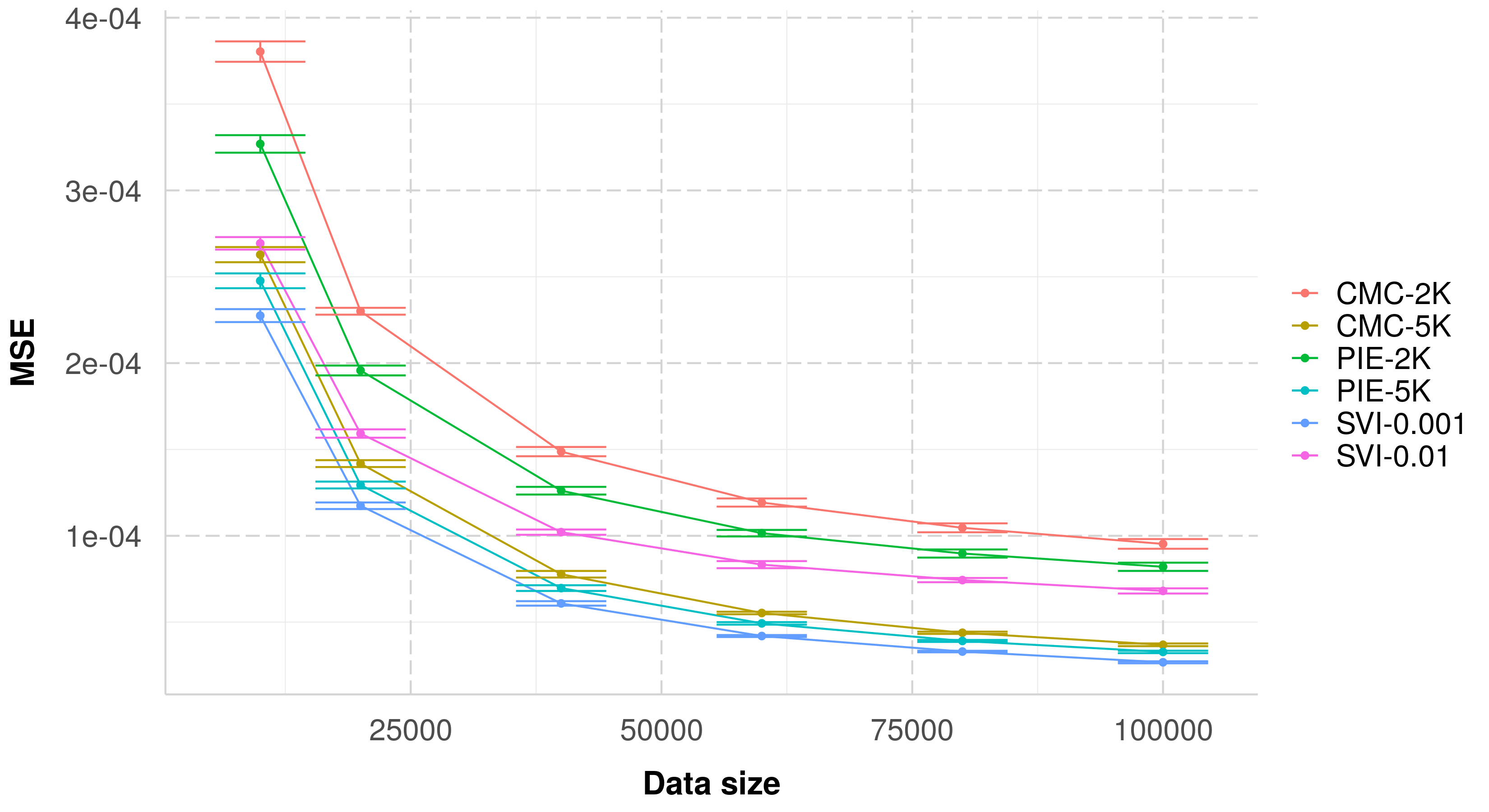
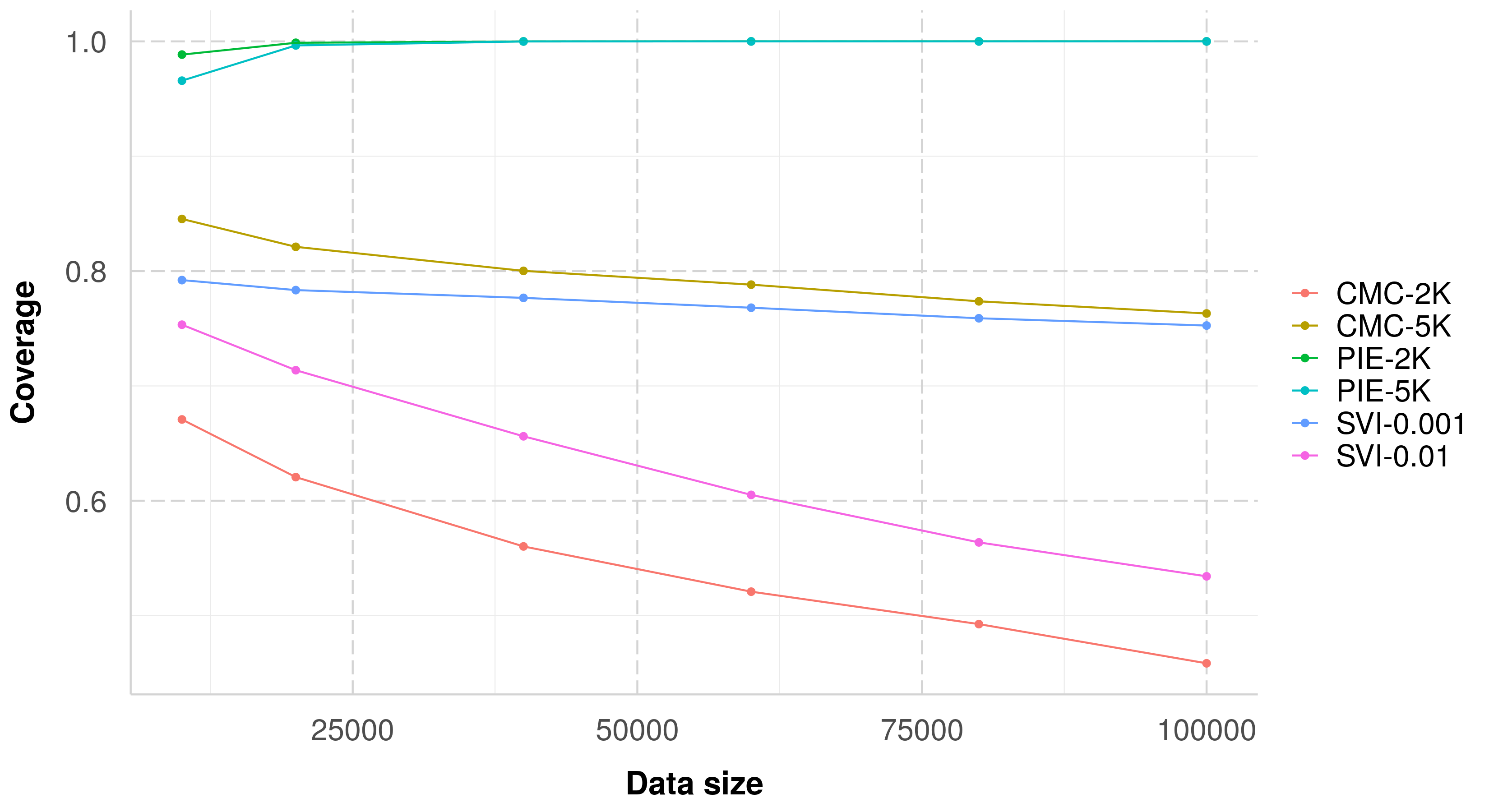
Figure 1: Simulation results for mean squared error (MSE) and coverage of the regression coefficients.

We hold the shard size constant for the posterior combination algorithms and instead increase the number of shards as $N$ increases. For example, the CMC-2K algorithms fix shard size at 2,000 data points and use 20 shards when the data size is 40,000 and 50 shards when the data size is 100,000, whereas CMC-5K uses 8 and 20 shards, respectively. This setup mimics the real-world situation where the limiting computational consideration is total run time and not the number of available machines for running the MCMC algorithms. For the SVI algorithms, we compare two constant step sizes of $0.001$ and $0.01$ and utilize a batch size of 100 for each iteration. We run the MCMC algorithms for 15,000 iterations per shard, using 10,000 of those iterations for burn in, and the SVI algorithms for 50,000 iterations.

The results for MSE and coverage for the regression coefficients are given in Figure 1. It can be seen that among the divide-and-conquer approaches, the PIE algorithm outperforms the CMC algorithm. It should be noted that, for both algorithms, better parameter estimation was achieved when shard size was fixed at 5K instead of 2K; this is not surprising since the convergence theory for both approaches requires that the size of each shard go to infinity. In terms of the average MSE of the regression coefficients, the SVI algorithm with step size $0.001$ outperforms all other algorithms; this provides support for the fact that SVI algorithms are appropriate to use when point estimates for the mean structure of the model are needed. In terms of coverage however, all algorithms do not achieve 95% coverage from 95% credible intervals. The CMC and SVI algorithms under-cover, while the PIE algorithm over-covers. For both the CMC and SVI algorithms, we see decreasing coverage as the data size increases, while for the PIE algorithms we see coverage go to one. We also investigated the length of the credible sets and saw that the CMC and SVI algorithms had intervals that narrowed as the sample size increased, whereas the interval length for the PIE algorithm remained constant.

Table 1: Mean absolute error (MAE) of the upper-triangular portion of the correlation matrix as data size increases. Average standard errors for the SVI algorithms are 0.0005, while the average standard errors for the divide-and-conquer approaches are 0.0002.

	N = 10K	N = 20K	N = 40K	N = 60K	N = 80K	N = 100K
CMC-2K	$0.0215$	$0.0165$	$0.0132$	$0.0118$	$0.0111$	$0.0106$
CMC-5K	$0.0181$	$0.0132$	$0.0096$	$0.0081$	$0.0072$	$0.0065$
PIE-2K	$0.0203$	$0.0157$	$0.0128$	$0.0118$	$0.0112$	$0.0107$
PIE-5K	$0.0175$	$0.0126$	$0.0091$	$0.0077$	$0.0069$	$0.0063$
SVI-0.001	$0.1107$	$0.1108$	$0.1097$	$0.1109$	$0.1117$	$0.1105$
SVI-0.01	$0.1109$	$0.1111$	$0.1097$	$0.1111$	$0.1120$	$0.1109$

Table 1 shows the mean absolute error of the upper triangular elements of the correlation matrix for the respective algorithms. Of note here is that the SVI algorithms perform poorly; the MAE does not improve as sample size increases. This may be due to the fact that the large correlation between ${{\bm{\mathbf{{\psi}}}}}_{n}$ and ${\bf z}_{n}$ is ignored in the mean-field assumption of the algorithm. On the other hand, the CMC and PIE algorithms improve in performance as the data size increases. As with the results for the regression coefficients, we see that increasing the size of a shard leads to improved estimation of the correlation matrix. Additionally, we also see that the PIE combination approach performs slightly better than the CMC approach.

In addition to the improved performance relative to CMC, PIE has an advantage with regards to the memory needed to combine posteriors. Since PIE estimates the posterior distribution by averaging quantiles, one can draw a large number of samples from each shard yet only store a small number of quantiles at which uncertainty quantification is of interest. Therefore, we use the PIE algorithm in our applied analyses in Section 5.

5 Applications

In this section we analyze a dataset of de-identified administrative claims for Medicare Advantage members in a research database from a single large US health insurance provider. The database contains medical claims for services submitted for third party reimbursement, available as International Classification of Diseases, Tenth Revision, Clinical Modification (ICD-10-CM). We use the ICD codes to identify chronic conditions via version twenty two of the Centers for Medicare & Medicaid Services’ (CMS) hierarchical condition categories (HCC), a provider’s specialty classification, and an individual’s demographic information in our analyses below. We show how the multivariate probit model (3), combined with divide-and-conquer MCMC, can be used to answer important questions using large medical claims data sets. First, we investigate patterns of chronic conditions in individuals with multiple HCCs to better identify areas of opportunity for targeted medical programs. Second, we investigate the urban-rural divide in healthcare, by analyzing provider utilization patterns of urban and rural individuals, relative to their suburban counterparts.

5.1 Co-morbid Conditions in the Medicare Advantage Population

We fit the multivariate probit model using an individual’s HCCs in 2018 as the response variable. As predictors, we use a member’s age, gender, and a flag for whether they were in a dual-eligible special needs plan (DSNP) during the year as predictors; DSNP enrollees are those enrolled in both Medicare Advantage and Medicaid. To find patterns in individuals who have multiple comorbidities, we restrict our attention to individuals who were diagnosed with at least four HCCs during the year and to the HCCs which were prevalent in at least one percent of the restricted population; the list of HCCs considered is shown in Figure 2. The final data set had approximately 500,000 individuals, 58 HCCs, and three predictors. We fit the model using 10 shards, 40 factors, and ran each sampler for 25,000 iterations, with 15,000 used for burn in. We combined individual shards using the PIE algorithm, and used the median of the correlation parameters as point estimates to visualize the correlation matrix.

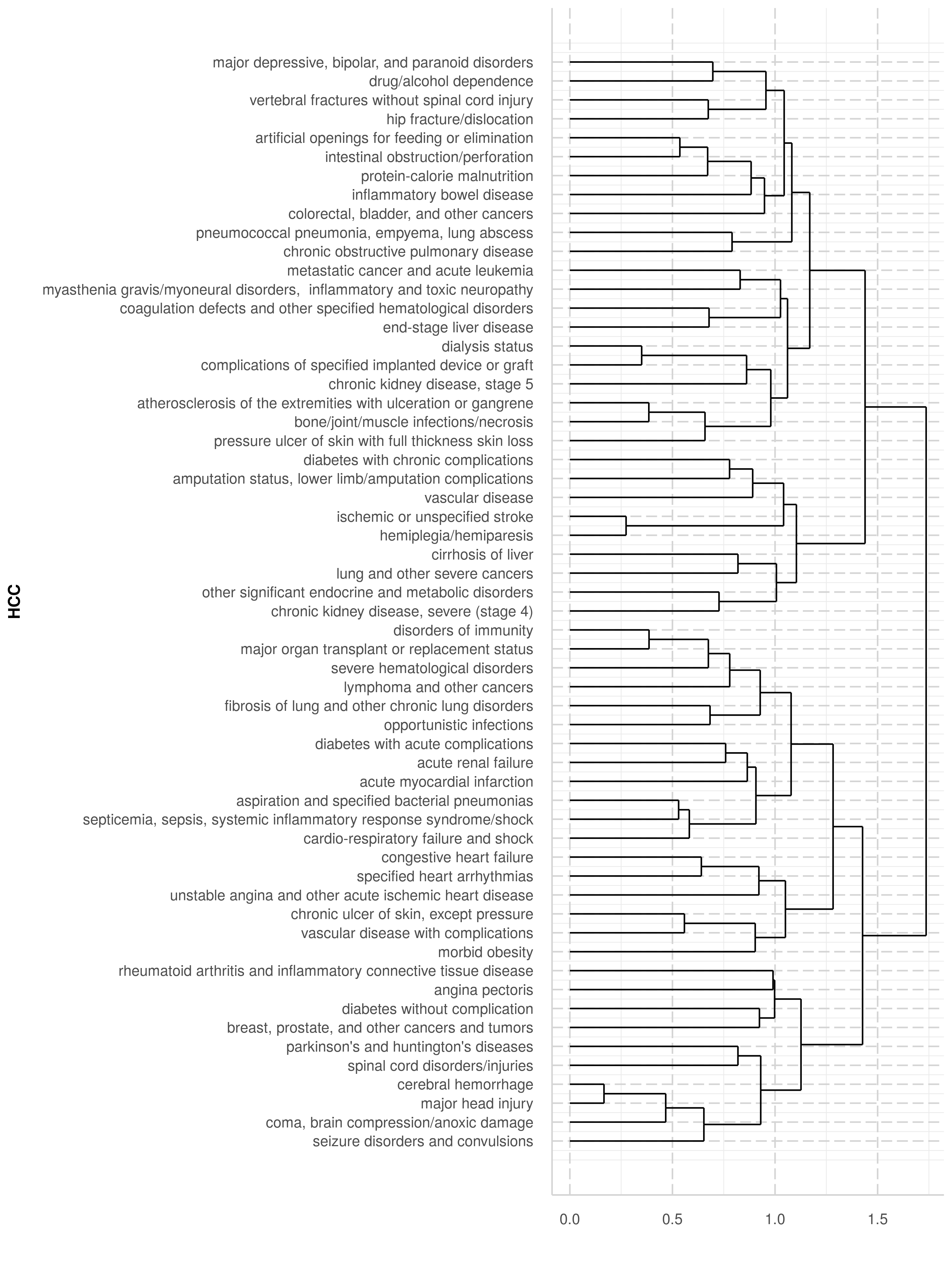
Figure 2: Dendrogram of the correlation matrix using one minus the correlation as a distance measure.

Figure 2 shows many interesting relationships among the HCCs. For example, a clear group is formed by the HCCs for aspiration and specified bacterial pneumonias, septicemia and sepsis, and cardio-respiratory failure. Examining these further, we found that the prevalence of these conditions in the overall population were approximately 5%, 16%, 22% and respectively, but when we subset to individuals who had aspiration and specified bacterial pneumonias, the rates of sepsis and cardio-respiratory failure increased to 49% and 59%, respectively. Alternatively, if we restrict our attention to individuals who had cardio-respiratory failure, the rates for sepsis and aspiration and specified bacterial pneumonias rise to 31% and 13%, respectively.

Another potentially interesting cluster is the group containing cerebral hemorrhage, major head injuries, coma, and seizure disorders. Upon investigation, we found that having a condition that falls in the coma HCC has an incidence of 1.5% in the population overall, whereas the incidence rate rises to 7.5% for individuals with a diagnosis of seizure disorders or convulsions. Additionally, the rates for cerebral hemorrhage were 2.3% in the general population and 8.5% for those who had seizure disorders or convulsions, while those for major head injury were 2.5% and 7.7%, respectively.

While more investigation is needed regarding the causal relationships within the two groups of HCCs above, we were able to apply the multivariate probit model to a large data set to visualize the relationships between HCCs. This approach can help practitioners identify groups for which intervention programs can be created. For example, it would be worth investigating the potential of head injury prevention programs for individuals with seizure disorders, or a program focused on reducing the rate of sepsis in individuals with aspiration and specified bacterial pneumonia.

5.2 Rural-Urban Divide in Specialty Care

In this section we try and understand how the utilization of specialists varies across rural, urban, and suburban populations, while controlling for an individual’s chronic conditions. As in the previous section, we apply the divide-and-conquer approach to a data set of Medicare Advantage enrollees. We restrict our attention to continuously enrolled individuals from 2018-2019 to get an accurate understanding of their chronic conditions and specialist visitation patterns in a particular year. For predictors, we use an individual’s age, gender, HCCs in 2018, a flag for whether they were enrolled in a DSNP plan at the start of 2019, and whether they lived in an urban, rural, or suburban area at the start of 2019. We regress these variables on indicators for whether or not an individual visited a particular specialty in 2019, and restrict the dimension of the response variable to specialties that were visited by 0.5% of individuals. Our final dataset consists of $3.1$ million individuals, with $60$ specialties, and $84$ predictors. As with the previous analysis, we fit the model using 40 factors.

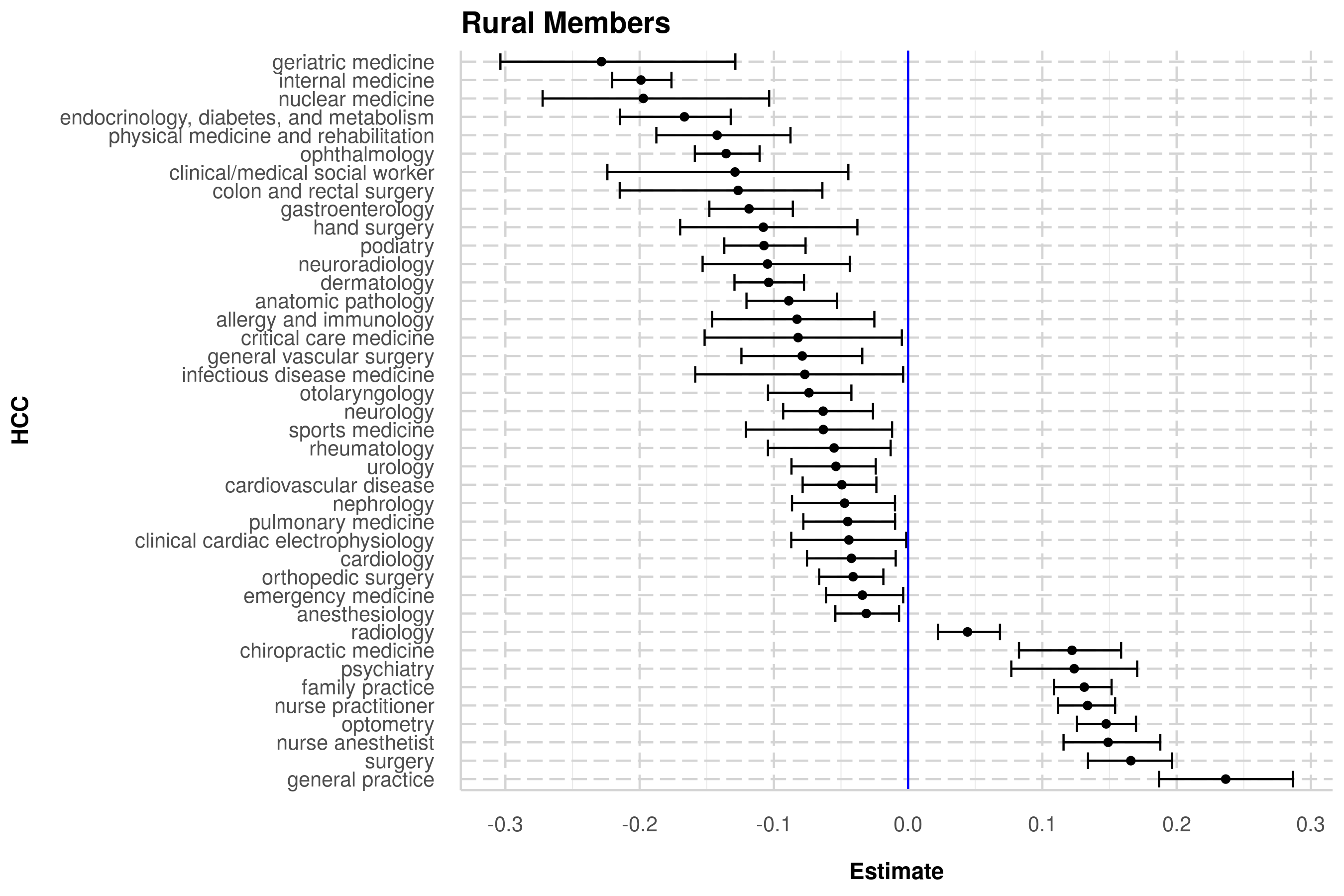
Figure 3: Specialties for which the 95% credible interval for the urban or rural regression coefficient did not include zero.

Figure 3 shows the specialties for which the 95% credible intervals for the urban and rural indicators did not contain zero, with suburban residence used as the baseline. Estimated regression coefficients greater than zero indicate that individuals in the group were more likely to visit a particular specialty, relative to suburban individuals, after accounting for their chronic conditions and demographics. It is interesting to note that many meaningful specialties have negative coefficients for rural individuals. For example, rural individuals were less likely to visit a doctor who specialized in endocrinology, diabetes and metabolism despite its prevalence in the general population. Additionally, rural individuals were less likely to visit ophthalmologists but more likely to visit optometrists, which may point to a mismatch of care since ophthalmologists can perform minor surgery for eye conditions. On the other hand, rural individuals had a higher utilization of nurse practitioners relative to suburban individuals; further investigation is warranted into whether this difference exists due to gaps in specialist care, and whether a larger than expected number of visits to nurse practitioners has a detrimental impact on the quality of care. Finally, we also note that rural individuals visited geriatric medicine specialists at a lower rate, which highlights the lack of geriatric specialty availability in rural areas despite the higher prevalence of older individuals (Hintenach et al., 2019).

While rural individuals visit nurse practitioners and family practice doctors at higher rates than their suburban counterparts, urban individuals visit them at relatively lower rates. Additionally, the relationship between ophthalmology and optometry is flipped for urban individuals, and urban individuals visit internal medicine physicians instead of those with family practice as their primary specialty. Another interesting point of note is that, relative to their suburban counterparts, urban individuals have a lower likelihood of visiting a physician assistant or a nurse practitioner. This under-utilization may point to opportunities for optimizing care, since nurse practitioners and physicians assistants tend to be cheaper per visit than other specialties. Finally, it should be noted that urban individuals visit endocrinologists at higher rates than their suburban counterparts, while rural individuals visit them at lower rates, which provides an actionable insight into a potential care gap between rural and urban diabetic enrollees.

6 Conclusion

In this paper, we show how a divide-and-conquer approach to MCMC can be utilized to analyze large scale medical databases. We conducted a simulation study comparing a stochastic variational algorithm with divide-and-conquer MCMC for the multivariate probit model, and showed that the stochastic variational approach underperforms in regards to estimation of the correlation matrix. We also compared the performance of two different posterior combination algorithms to understand their behavior as shard size remains fixed and the number of samples increases. Our approach of combining divide-and-conquer MCMC with the multivariate probit model drastically reduces the run time of the multivariate probit Gibbs sampler when applied to a large dataset.

In our applications, we explored two important questions for the health care system. First, we found patterns of multimorbidity that can be used to create health care programs tailored to specific disease profiles. Second, we investigated how utilization of particular specialties differs between urban, suburban, and rural individuals, and found that a potential gap in care exists for diabetic individuals. A limitation of our analysis is that we fixed the number of factors in our MCMC algorithms; a full Bayesian analysis would require us to use model averaging to incorporate results from a differing number of factors. However, it is unclear how to conduct model averaging in the context of a divide-and-conquer approach, since it is an open question as to whether model averaging be conducted at the shard level or at the combined posterior level. We posit that the appropriate level to combine different models would be the individual shard level, which would allow the optimal number of factors to vary by subsample. A detailed study of model averaging in the context of divide-and-conquer MCMC is beyond the scope of this work, and we leave the question to be addressed by future research.

While we focused our attention on analyzing multivariate binary datasets, we hope that future research uses the latent factor model framework with divide-and-conquer MCMC to extend our approach to multivariate count data and multivariate mixed (binary, count, continuous) data. For example, it would be interesting to analyze the number of visits to different specialties, or to simultaneously predict the number of hospitalizations, the onset of new diagnoses, and total cost. Finally, we also aim to incorporate a greater number of predictors into our analyses (lab results, medications), and leverage GPU clusters to conduct variable selection on large scale medical databases.

References

- Abadi et al. (2015) Martín Abadi, Ashish Agarwal, Paul Barham, Eugene Brevdo, Zhifeng Chen, Craig Citro, Greg S. Corrado, Andy Davis, Jeffrey Dean, Matthieu Devin, Sanjay Ghemawat, Ian Goodfellow, Andrew Harp, Geoffrey Irving, Michael Isard, Yangqing Jia, Rafal Jozefowicz, Lukasz Kaiser, Manjunath Kudlur, Josh Levenberg, Dan Mané, Rajat Monga, Sherry Moore, Derek Murray, Chris Olah, Mike Schuster, Jonathon Shlens, Benoit Steiner, Ilya Sutskever, Kunal Talwar, Paul Tucker, Vincent Vanhoucke, Vijay Vasudevan, Fernanda Viégas, Oriol Vinyals, Pete Warden, Martin Wattenberg, Martin Wicke, Yuan Yu, and Xiaoqiang Zheng. TensorFlow: Large-scale machine learning on heterogeneous systems, 2015. URL http://tensorflow.org/. Software available from tensorflow.org.
- Ashford and Sowden (1970) JR Ashford and RR Sowden. Multi-variate probit analysis. Biometrics, pages 535–546, 1970.
- Baker et al. (2019) Jack Baker, Paul Fearnhead, Emily B Fox, and Christopher John Nemeth. sgmcmc: An r package for stochastic gradient markov chain monte carlo. Journal of Statistical Software, 91(3):1–27, 2019.
- Bardenet et al. (2017) Rémi Bardenet, Arnaud Doucet, and Chris Holmes. On markov chain monte carlo methods for tall data. The Journal of Machine Learning Research, 18(1):1515–1557, 2017.
- Betancourt (2017) Michael Betancourt. A conceptual introduction to hamiltonian monte carlo. arXiv preprint arXiv:1701.02434, 2017.
- Bhattacharya and Dunson (2011) Anirban Bhattacharya and David B Dunson. Sparse bayesian infinite factor models. Biometrika, pages 291–306, 2011.
- Blei et al. (2017) David M. Blei, Alp Kucukelbir, and Jon D. McAuliffe. Variational inference: A review for statisticians. Journal of the American Statistical Association, 112(518):859–877, 2017. doi: 10.1080/01621459.2017.1285773. URL https://doi.org/10.1080/01621459.2017.1285773.
- Brantley et al. (2020) Halley L Brantley, Joseph Guinness, Eric C Chi, et al. Baseline drift estimation for air quality data using quantile trend filtering. Annals of Applied Statistics, 14(2):585–604, 2020.
- Chib and Greenberg (1998) Siddhartha Chib and Edward Greenberg. Analysis of multivariate probit models. Biometrika, 85(2):347–361, 06 1998. ISSN 0006-3444. doi: 10.1093/biomet/85.2.347. URL https://doi.org/10.1093/biomet/85.2.347.
- Cyr et al. (2019) Melissa E Cyr, Anna G Etchin, Barbara J Guthrie, and James C Benneyan. Access to specialty healthcare in urban versus rural us populations: a systematic literature review. BMC health services research, 19(1):1–17, 2019.
- Hahn et al. (2012) P Richard Hahn, Carlos M Carvalho, and James G Scott. A sparse factor analytic probit model for congressional voting patterns. Journal of the Royal Statistical Society: Series C (Applied Statistics), 4(61):619–635, 2012.
- Hing and Hsiao (2014) Esther Hing and Chun-Ju Hsiao. State Variability in Supply of Office-based Primary Care Providers, United States, 2012. Number 151. US Department of Health and Human Services, Centers for Disease Control and …, 2014.
- Hintenach et al. (2019) Annette Hintenach, Oren Raphael, and William W Hung. Training programs on geriatrics in rural areas: a review. Current geriatrics reports, 8(2):117–122, 2019.
- Hoffman et al. (2013) Matthew D Hoffman, David M Blei, Chong Wang, and John Paisley. Stochastic variational inference. The Journal of Machine Learning Research, 14(1):1303–1347, 2013.
- Huang and Gelman (2005) Zaijing Huang and Andrew Gelman. Sampling for bayesian computation with large datasets. Available at SSRN 1010107, 2005.
- James and Cossman (2017) Wesley James and Jeralynn S Cossman. Long-term trends in black and white mortality in the rural united states: Evidence of a race-specific rural mortality penalty. The Journal of Rural Health, 33(1):21–31, 2017.
- Kleiner et al. (2014) Ariel Kleiner, Ameet Talwalkar, Purnamrita Sarkar, and Michael I Jordan. A scalable bootstrap for massive data. Journal of the Royal Statistical Society: Series B: Statistical Methodology, pages 795–816, 2014.
- Lawrence et al. (2008) Earl Lawrence, Derek Bingham, Chuanhai Liu, and Vijayan N Nair. Bayesian inference for multivariate ordinal data using parameter expansion. Technometrics, 50(2):182–191, 2008.
- Li et al. (2017) Cheng Li, Sanvesh Srivastava, and David B Dunson. Simple, scalable and accurate posterior interval estimation. Biometrika, 104(3):665–680, 2017.
- Ma et al. (2015) Yi-An Ma, Tianqi Chen, and Emily Fox. A complete recipe for stochastic gradient mcmc. In Advances in Neural Information Processing Systems, pages 2917–2925, 2015.
- McCulloch and Rossi (1994) Robert McCulloch and Peter E Rossi. An exact likelihood analysis of the multinomial probit model. Journal of Econometrics, 64(1-2):207–240, 1994.
- Mehrotra and Maity (2021) Suchit Mehrotra and Arnab Maity. Variational inference for shrinkage priors: The r package vir. arXiv preprint arXiv:2102.08877, 2021.
- Minsker et al. (2014) Stanislav Minsker, Sanvesh Srivastava, Lizhen Lin, and David Dunson. Scalable and robust bayesian inference via the median posterior. In International conference on machine learning, pages 1656–1664, 2014.
- Neiswanger et al. (2013) Willie Neiswanger, Chong Wang, and Eric Xing. Asymptotically exact, embarrassingly parallel mcmc. arXiv preprint arXiv:1311.4780, 2013.
- Newcomer et al. (2011) Sophia R Newcomer, John F Steiner, and Elizabeth A Bayliss. Identifying subgroups of complex patients with cluster analysis. The American journal of managed care, 17(8):e324–32, 2011.
- Prados-Torres et al. (2014) Alexandra Prados-Torres, Amaia Calderón-Larranaga, Jorge Hancco-Saavedra, Beatriz Poblador-Plou, and Marjan van den Akker. Multimorbidity patterns: a systematic review. Journal of clinical epidemiology, 67(3):254–266, 2014.
- Scott et al. (2016) Steven L Scott, Alexander W Blocker, Fernando V Bonassi, Hugh A Chipman, Edward I George, and Robert E McCulloch. Bayes and big data: The consensus monte carlo algorithm. International Journal of Management Science and Engineering Management, 11(2):78–88, 2016.
- Srivastava et al. (2015) Sanvesh Srivastava, Volkan Cevher, Quoc Dinh, and David Dunson. Wasp: Scalable bayes via barycenters of subset posteriors. In Artificial Intelligence and Statistics, pages 912–920, 2015.
- Tabet (2007) Aline Tabet. Bayesian inference in the multivariate probit model. PhD thesis, University of British Columbia, 2007.
- Taylor-Rodríguez et al. (2017) Daniel Taylor-Rodríguez, Kimberly Kaufeld, Erin M. Schliep, James S. Clark, and Alan E. Gelfand. Joint species distribution modeling: Dimension reduction using dirichlet processes. Bayesian Anal., 12(4):939–967, 12 2017. doi: 10.1214/16-BA1031. URL https://doi.org/10.1214/16-BA1031.
- Terenin et al. (2019) Alexander Terenin, Shawfeng Dong, and David Draper. Gpu-accelerated gibbs sampling: a case study of the horseshoe probit model. Statistics and Computing, 29(2):301–310, 2019.
- Violan et al. (2014) Concepció Violan, Quintí Foguet-Boreu, Gemma Flores-Mateo, Chris Salisbury, Jeanet Blom, Michael Freitag, Liam Glynn, Christiane Muth, and Jose M Valderas. Prevalence, determinants and patterns of multimorbidity in primary care: a systematic review of observational studies. PloS one, 9(7):e102149, 2014.
- Weisgrau (1995) Sheldon Weisgrau. Issues in rural health: access, hospitals, and reform. Health care financing review, 17(1):1, 1995.
- Welling and Teh (2011) Max Welling and Yee W Teh. Bayesian learning via stochastic gradient langevin dynamics. In Proceedings of the 28th international conference on machine learning (ICML-11), pages 681–688, 2011.
- Xu et al. (2017) Zheng Xu, Gavin Taylor, Hao Li, Mário AT Figueiredo, Xiaoming Yuan, and Tom Goldstein. Adaptive consensus admm for distributed optimization. In Proceedings of the 34th International Conference on Machine Learning-Volume 70, pages 3841–3850, 2017.