blackNonlinear reconstruction of features in the primordial power spectrum from large-scale structure

Abstract

Potential features in the primordial power spectrum have been searched for in galaxy surveys in recent years since these features can assist in understanding the nature of inflation. The null detection to date suggests that any such features should be fairly weak, and next-generation galaxy surveys, with their unprecedented sizes and precisions, are in a position to place stronger constraints than before. However, even if such primordial features once existed in the early Universe, they would have been significantly damped blackin the nonlinear regime at low redshift due to structure formation, which makes them difficult to be directly detected in real observations. A potential way to tackle this challenge for probing the features is to undo the cosmological evolution, i.e., using reconstruction to obtain an approximate linear density field. By employing a blackset of N-body simulations, here we show that a recently-proposed nonlinear reconstruction algorithm can effectively retrieve damped oscillatory features from blackhalo catalogues and improve the accuracy of the measurement of feature parameters (assuming that such primordial features do exist). We do a Fisher analysis to forecast how blacknonlinear reconstruction affects the constraining power, and find that it can lead to significantly more robust constraints on the feature amplitude for a DESI-like survey. blackComparing blacknonlinear reconstruction with other ways of improving constraints, such as increasing the survey volume and range of scales, this shows that it is possible to achieve what the latter do, but at a lower cost.

1 Introduction

Inflation, the most successful theory to solve the problems of the hot Big Bang model and to explain the seeding of the observed large-scale structures today, plays a crucial role in the development of modern cosmology. The single-field blackslow-roll inflation (Guth, 1981; Linde, 1982; Albrecht & Steinhardt, 1982) predicts that primordial density fluctuations obey Gaussian statistics and the corresponding power spectrum follows a simple power law, which is favoured by the cosmic microwave background (CMB) data released by the WMAP (Peiris et al., 2003; Spergel et al., 2007; Komatsu et al., 2009; Hinshaw et al., 2013) and Planck (Ade et al., 2014a; Ade et al., 2016b; Akrami et al., 2020b) collaborations.

However, the physical origin of the inflaton fieldblack, which is believed to have driven inflationblack, is not fully understood yet, and the fact that the very high energy blackscale in the early Universe makes it an ideal place to blackprobe the imprints of the laws of fundamental physics offers blackthe possibility that new physics can be revealed by cosmological observations of the large-scale structure black(LSS). blackCertain sophisticated models blackof inflation and its alternatives blackdeveloped over the last decades blackpredict scale-dependent features in the power spectrum of primordial density fluctuations (see, e.g., Bartolo et al., 2004; Chen, 2010; Chluba et al., 2015; Slosar et al., 2019, for some reviews). blackSuch ‘feature models’ blackcan be mainly classified into three types blackwith specific templates of oscillations added to the scale-invariant primordial power spectrum, each of which can be attributed to various mechanisms (see, e.g., Chen, 2010; Chluba et al., 2015; Slosar et al., 2019, for some reviews). ‘Sharp-feature’ models blackhave sinusoidal wiggles blackin the power spectrum, $P(k)$, that oscillate linearly in wavenumber $k$ blackat a fixed frequency, $\omega$, which can be generated by a minimal local singularity such as a step in the inflationary potential blackthat breaks the slow-roll condition (e.g., Starobinsky, 1992; Adams et al., 2001; Chen et al., 2007; Hazra et al., 2010; Adshead et al., 2012; Hazra et al., 2014), or produced in particular cases of multi-field models of inflation (e.g., Achucarro et al., 2011; Gao et al., 2012). Another type is blackthe ‘resonant-feature’ model whose oscillatory features are in logarithmic $k$, which can be realised in, e.g., the axion monodromy inflation (Flauger et al., 2010; Flauger & Pajer, 2011), or brane inflation (Bean et al., 2008), blackmodels. The last type is blackthe so-called standard clock signal, which is a combination of the previous two feature models (e.g., Chen, 2012; Chen & Namjoo, 2014; Chen et al., 2015).

blackThese feature models have been continuously tested with the updated release of data from the Planck mission (Ade et al., 2014b, 2016a; Akrami et al., 2020a), blackbut none of them blackhas been found to be preferable to the blackscale-invariant power spectrum predicted by simple single-field slow-roll inflation models so far, which suggests that such features should be fairly weak if they do exist. Since the primordial features are not only imprinted in the CMB, blackbut some of them can also leave a signature in the matter blackand galaxy distribution, future LSS surveys, such as Euclid (Racca et al., 2016), DESI (DESI Collaboration et al., 2016), SPHEREx (Doré et al., 2014) and LSST (Ivezić et al., 2019), will provide the opportunity to search for, blackor tighten the constraints on, them, complementary to CMB data (e.g., Huang et al., 2012; Chen et al., 2016; Ballardini et al., 2016; Palma et al., 2018; L’Huillier et al., 2018; Ballardini et al., 2018; Zeng et al., 2019). blackMore recently, this idea has been put into practice by making forecast (e.g., Beutler et al., 2019; Ballardini et al., 2020; Debono et al., 2020) or performing real LSS data analysis (Beutler et al., 2019).

However, any feature imprinted in the primordial density or curvature field by inflation is subject to the impact of cosmic evolution that blacklast until today. In particular, even if blacksuch primordial features once existed in the very early Universe, they would have been blackmodified in the late-time Universe due to nonlinear structure formation. Meanwhile, the available information on large scales, where the evolution can be described by linear blackperturbation theory, is limited due to the cosmic varianceblack, i.e., the poor statistics caused by the finite number of Fourier modes probed in that regime. This can affect the confidence level at which to measure or constrain these features. blackIn order to blackmaximally extract useful information from the blackobserved galaxy distributions, several studies of the primordial features in the nonlinear regime has been conducted. blackVasudevan et al. (2019); Beutler et al. (2019) analytically computed the damping effect by gravitational nonlinearities, making a considerable contribution to the forecast of constraints on primordial feature from future galaxy surveys. Ballardini et al. (2020) employed N-body simulations to show a compatible nonlinear damping effect with the analytic results above to leading order. Beutler et al. (2019) and Ballardini et al. (2020) made forecasts for future galaxy surveys by taking the damping effect into account. Besides, Beutler et al. (2019) performed the first LSS data analysis for the primordial features, which showed that LSS can surpass the CMB as a probe of such features. Furthermore, Vlah et al. (2016) and Chen et al. (2020) showed that different perturbation theories, including Lagrangian and Eulerian perturbation theories and the effective field theory, can model the nonlinear evolution of primordial features well for $k\lesssim 0.25\ h\rm Mpc^{-1}$ at $z=1$ and for $k\lesssim 0.2\ h\rm Mpc^{-1}$ at $z=0$, but no oscillatory features survive past $k\approx 0.5\ h\rm Mpc^{-1}$. Thus, it would be beneficial to blackdevelop other approaches which can potentially allow us to exploit the LSS data in the range of scales, $0.2\lesssim{k/(h{\rm Mpc}^{-1})}\lesssim 0.5$ blackeven at low redshifts.

A potential method blackmentioned in Vasudevan et al. (2019); Ballardini et al. (2020) and implemented in Beutler et al. (2019) to address the issue blackof nonlinear damping and further improve the constraints on primordial features is to undo the cosmological evolution in a process called reconstruction, which can partially blackretrieve the initial density field and blacktherefore the information that existed blackthere. A well-known example is the reconstruction of baryonic acoustic oscillation (BAO) features, which sharpens these features in the galaxy correlation function which provides a standard ruler for distance measurements (e.g., Eisenstein et al., 2007; Kazin et al., 2014; Schmittfull et al., 2015; Zhu et al., 2017; Wang et al., 2017; Shi et al., 2018; Sarpa et al., 2019; Mao et al., 2021). blackblackWhile reconstructing the primordial power spectrum from observed blackgalaxies has been shown to be beneficial for probing the primordial features blackfrom LSS data (Beutler et al., 2019), blackthis study made use of one particular (the standard) reconstruction method, and it will be interesting to also assess how other reconstruction methods work in this regard.

In this work, as a first step towards assessing the potential benefit of blacknonlinear reconstruction, we assume additional simple oscillatory features in the power-law primordial power spectrum. By utilising a blacksmall set of N-body simulations, we study the performance of blackthe nonlinear reconstruction algorithm proposed recently by Shi et al. (2018); Birkin et al. (2019) blackin retrieving the damped primordial features from the blackhalo catalogues. In particular, blackby quantifying blackthis damping blackcaused by structure formation based on the functional form in Vasudevan et al. (2019); Beutler et al. (2019), we will carry out parameter fittings to the damped and reconstructed wiggles, blackthe comparison of which allows us to assess whether nonlinear reconstruction can lead to more robust constraints on the feature parameters. To investigate the impact of blacknonlinear reconstruction in real galaxy surveys, we also forecast the constraints on the feature parameters for blacka DESI-like survey using the Fisher matrix approach, and compare the cases with and without reconstruction.

This paper is organised as follows: in Section 2 we describe the model of primordial features, the simulations used in this work, and the methodology of assessing the performance of the nonlinear reconstruction method to retrieve the damped primordial features due to structure formation. In Section 3 we give more details on the approach used to forecast the constraints on the feature parameters for the DESI-like survey. In Section 4 we show the results of nonlinear reconstruction and forecast and discuss the implications of them. Finally, in Section 5 we conclude our findings and discuss potential future improvements.

2 Methodology

We start with presenting the primordial power spectrum models with oscillatory features that we adopt in this paper for illustration purpose. We then describe the simulation runs for these models. It is followed by a brief review of the nonlinear reconstruction method which will be used to recover the small-scale oscillation features from evolved dark matter and halo fields. Finally, we describe the analytic model to quantify the features measured in the power spectrum before giving the details of the Fisher matrix forecast in the next section.

2.1 Models of featured primordial power spectrum

We take a powerlaw-type primordial power spectrum to be our fiducial no-wiggle model black(note that the BAO wiggles are still included), given by

$$P_{\rm nw}^{\rm\textcolor{black}{ini}}(k)=A_{s}\bigg{(}\frac{k}{k_{\ast}}\bigg{)}^{n_{s}-1},$$ (1)

where $k$ is the comoving wavenumber, $A_{s}$ and $n_{s}$ are respectively the scalar amplitude and spectral index with the pivot scale given by $k_{\ast}=0.05\ \rm Mpc^{-1}$. blackTo explore whether the nonlinear reconstruction algorithm blackemployed in this paper can lead to improvements compared with the unreconstructed cases in Ballardini et al. (2020), we consider blackfour wiggled models that are based on the template of the sharp feature model (Slosar et al., 2019), i.e., oscillations in linear $k$, given by

$$P_{\rm w}^{\rm ini}(k)=P_{\rm nw}^{\rm ini}(k)\big{[}1+A\textcolor{black}{\cos(\omega k^{m}+\phi)}\big{]},$$ (2)

where $A$, $\omega$ and $\phi$ are respectively the amplitude, frequency and phase of the oscillation. We extend the sharp feature model by introducing $m$ for a particular purpose explained later; when $m=1$, Eq. (2) is related to the Eq. (2.1) in Ballardini et al. (2020).

Note that even if the primordial features exist, they could be more complicated than any phenomenological models that we are currently using. For now, we cannot determine the precise form of the features, thus we aim at something narrow, which is assuming that we know the functional form and verifying if blacknonlinear reconstruction can improve the accuracy of blackmeasuring the feature parameters.

The oscillation parameters of the blackfive models are listed in Table 1. blackNote that the frequencies of the wiggled models here are in units of ${\rm Mpc}^{m}$ due to $m$ introduced above. The initial oscillations of the blackfour wiggled models are shown in the red dashed lines in the right panel of Fig. 1, where we have presented the difference between $P_{\rm w}^{\rm\textcolor{black}{ini}}$ and $P_{\rm nw}^{\rm\textcolor{black}{ini}}$. Within our interested range of scales, $k=(0.05-0.5)\ h\rm Mpc^{-1}$, blackModel 1 has the first peak at the smallest scale, followed by Model 2 and Model 3, the frequency used in Model 3 is the same as BAO frequency. Model 4 is particularly adopted to have the first two peaks at the same positions of the first and third peaks of Model 2. The reason why this special model is designed will be explained in Section 4.2. By comparing the reconstructed wiggles of the blackfour wiggled models later, we would be able to comprehend the effect of the blacknonlinear reconstruction method on different scales.

2.2 N-body simulations

In the regime of linear perturbations, the primordial wiggles preserve their shapes and amplitude $P_{\rm w}^{\rm\textcolor{black}{ini}}/P_{\rm nw}^{\rm\textcolor{black}{ini}}$. However, nonlinear large-scale structure evolution will change this behaviour, leading to damping of $P_{\rm w}^{\rm\textcolor{black}{ini}}/P_{\rm nw}^{\rm\textcolor{black}{ini}}$ at late times. This makes it harder to measure the properties of these primordial oscillations blackdirectly from an evolved density field, even more so for a late-time tracer (e.g., galaxy blackor halo) field. In order to quantify such effects, N-body cosmological simulations can prove to be a useful tool.

We have run blackfive simulation runs including the no-wiggle model and blackfour wiggled models. First we assume a flat universe and adopt Planck 2018 cosmology, with $h=0.674$, $\rm\Omega_{m}=0.3135$, $\Omega_{c}h^{2}=0.120$, $\Omega_{b}h^{2}=0.0224$, $\rm\Omega_{\Lambda}=0.6865$, $n_{s}=0.965$ and $A_{s}=2\times 10^{-9}$ (Aghanim et al., 2020). The value of $\sigma_{8}$ is approximately 0.79 though it varies a little bit across different models. We then customise the function of the primordial power spectrum in the Einstein-Boltzmann solver code camb (Lewis & Challinor, 2011) to be Eq. (1) for the no-wiggle model and Eq. (2) for the wiggled models. We calculate the linear theory matter power spectrum at $z=49$ using this version of the camb code, which is used as the input matter power spectrum for the publicly available code 2lptic (Crocce et al., 2006) to generate the initial conditions used for the N-body simulations. In the left panel of Fig. 1 we compare the initial matter power spectrum given by camb and the matter power spectrum measured from the initial conditions generated using 2lptic; it can be seen that they are in good agreement for all models within the range of scales of our interest (the blowing up at small scales is due to the finite particle resolution).

To more conveniently describe the oscillatory features for the wiggled models, as mentioned above, we define the relative wiggle pattern as

$$\textcolor{black}{O}_{\rm rw}^{\rm\textcolor{black}{ini}}(k)=\frac{P_{\rm w}^{\rm\textcolor{black}{ini}}(k)}{P_{\rm nw}^{\rm\textcolor{black}{ini}}(k)}-1,$$ (3)

which are shown in the right panel of Fig. 1. This indicates that the oscillatory features blackhave been reliably created in the initial conditions of the simulations blackwithin our interested range of scales, blacke.g., $k\lesssim 0.5$ $h\mathrm{Mpc}^{-1}$.

Next, we run the simulations using the parallel N-body code ramses (Teyssier, 2002) which is based on the adaptive mesh refinement (AMR) technique. Each simulation is performed with $N=1024^{3}$ dark matter particles in a box of size $1024\ h^{-1}\rm Mpc$, and we output four snapshots at different redshifts, respectively as $z=0$, $0.5$, $1$, and $1.5$. For each snapshot, we use the halo finder rockstar (Behroozi et al., 2013) to identify the haloes with the definition of the halo mass $M_{200c}$, where $M_{200c}$ is the mass within a sphere whose average density is 200 times the critical density. Since the low-mass haloes are unable to be fully probed due to the limited simulation resolution, we measure the cumulative halo mass functions (cHMFs) from the main haloes with more than $100$ particles to check the validity of the simulation, which show very good agreement with the analytic formulae in Tinker et al. (2008). For each snapshot we establish one dark matter particle catalogue (hereafter DM) and two blackhalo catalogues respectively with the number density of $1\times 10^{-3}(h^{-1}\rm Mpc)^{-3}$ (hereafter H1) and $5\times 10^{-4}(h^{-1}\rm Mpc)^{-3}$ (hereafter H2). Both host haloes and subhaloes are included in the halo catalogues. blackThe number density of $5\times 10^{-4}(h^{-1}\rm Mpc)^{-3}$ is chosen to be an approximate value according to the current observations such as CMASS or LOWZ despite not being exactly the same, and $1\times 10^{-3}(h^{-1}\rm Mpc)^{-3}$ is a representative value of emission line galaxies (ELGs) in DESI survey; these choices are also somehow limited by the resolution of our simulations, though the use of the dark matter density field serves as a catalogue that has a much larger number density. Many realistic mock galaxy catalogues would give something between H1 and DM.

We achieve the number density by applying a mass cutoff, i.e., neglecting the haloes with smaller masses than the cutoff. By using the power spectrum estimator tool powmes (Colombi & Novikov, 2011), we measure the nonlinear matter power spectrum from DM and nonlinear halo power spectrum separately from H1 and H2. Finally, we take the ratio of the power spectrum of the wiggled models to the corresponding power spectrum of the no-wiggle model to obtain the quantity $\textcolor{black}{O}_{\rm rw}$ for all cases.

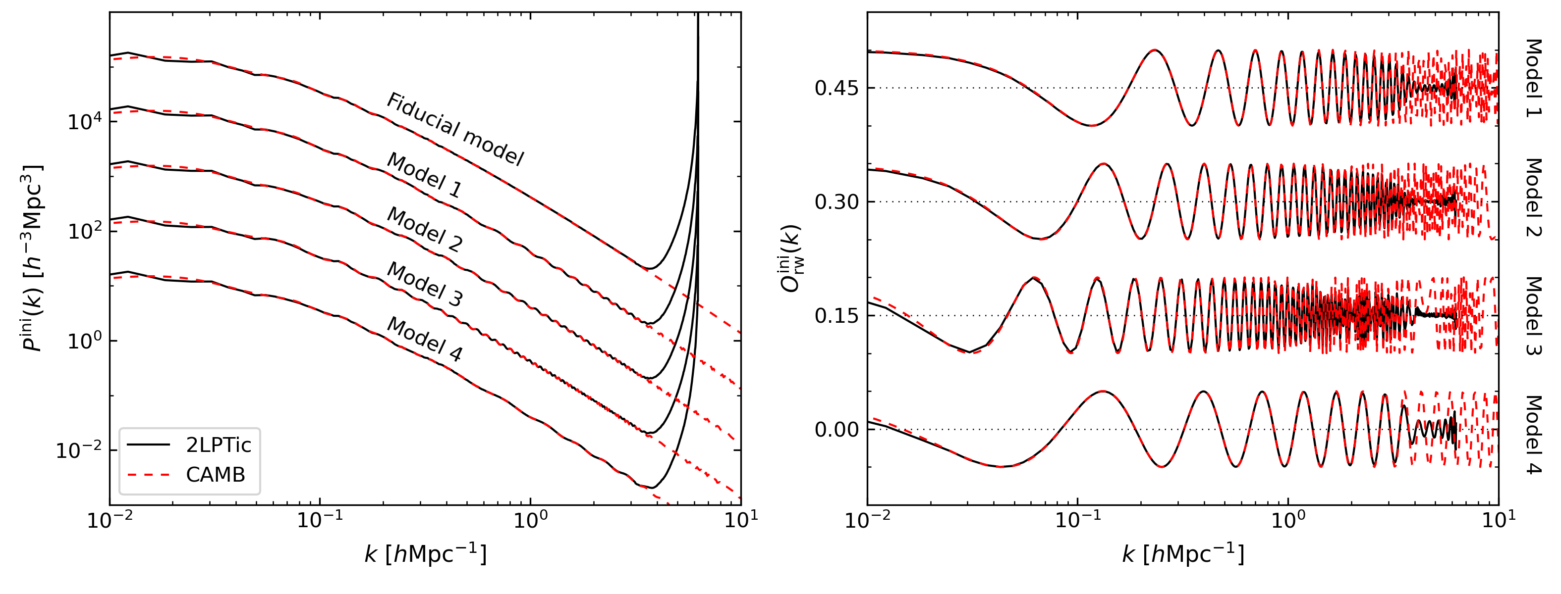
Figure 1: [Colour Online] The left panel shows the comparison between the initial matter power spectra given by camb (red dashed lines) and the matter power spectra measured from the initial conditions of the simulations generated using 2lptic (black lines), from the top down they are respectively the fiducial model, Model 1, Model 2, Model 3 blackand Model 4, each model is shifted upwards by a factor of $10$ successively to avoid the clutter of all curves. The right panel shows the $\textcolor{black}{O}_{\rm rw}^{\rm ini}$ results, cf., Eq. (3), obtained from the left panel for the four wiggled models, for instance, the top curve shows the ratio of Model 1 to the fiducial model, followed by the ones for Model 2, Model 3 blackand Model 4 downwards; each model is shifted upwards by a constant of $0.15$ successively for the same reason as above.

Table 1: The oscillation parameters used for the no-wiggle model and blackfour wiggled models. Columns respectively denote (1) the power of the comoving wavenumber; (2) the amplitude, (3) frequency and (4) phase of the oscillation.

	$m$	$A$	$\omega$	$\phi/\pi$
			black$[{\rm Mpc}^{m}]$
Fiducial		$0$
Model $1$	$1$	$0.05$	black$40$	$0$
Model $2$	$1$	$0.05$	black$70$	$0$
Model $3$	$1$	$0.05$	black$150$	$0$
Model $4$	$0.631$	$0.05$	black$28.9$	$0$

2.3 Reconstruction

In order to partially blackretrieve the primordial features damped during structure formation, we perform reconstruction of the initial density field from the late-time density field using the nonlinear reconstruction algorithm described in Shi et al. (2018). This reconstruction method is based on mass conservation. Without assuming a cosmological model or having free parameters except the size of the mesh used to calculate the density field, it employs multigrid Gauss-Seidel relaxation to solve the nonlinear partial differential equation which governs the mapping between the initial Lagrangian and final Eulerian coordinates of particles in evolved density fields. Previous tests show that the reconstructed density field is over $\sim 80\%$ correlated with the initial density field for $k\lesssim 0.6\ h\rm Mpc^{-1}$, if reconstruction is performed on the dark matter density field, which cover the scales of our interest, but the performance becomes poorer when the method is instead applied on the density fields calculated from sparse tracers (Birkin et al., 2019; Wang et al., 2020; Liu et al., 2020). This method is implemented in a modified version of the ecosmog code (Li et al., 2012; Li et al., 2013), which itself is based on ramses.

We reconstruct the initial density field separately from the catalogues DM, H1 and H2 for each snapshot. The halo catalogues, which contain both main and subhaloes, are assumed to be the same as mock galaxy catalogues hereafter unless otherwise stated. The procedure for the reconstruction from the halo catalogue is principally similar to that from the dark matter particle catalogue, apart from two things at the beginning. One is that we prepare the Gadget-format particle data for the ecosmog code in two ways. The halo catalogue is directly written into Gadget-format tracer particles due to its small number density. However, the very large number of the simulation particles, along with their strongly non-uniform spatial distribution, in the dark matter particle catalogues, leads to the requirement of large memory footprint when processing the data. To avoid this problem, we use the publicly available dtfe code (Cautun & van de Weygaert, 2011), based on Delaunay tessellation, to calculate the density field on a regular mesh with $512^{3}$ cells employing the triangular shaped cloud (TSC) mass assignment scheme; then the mesh cells are regarded as uniformly-distributed fake particles with different masses, which are transformed to Gadget format that can be directly read by ecosmog.

The other particular thing is that we calculate the linear halo bias used for the reconstruction from the halo catalogue. The estimate of the halo bias is based on the relation

$$b_{1}(r)=\frac{\xi_{\rm hh}(r)}{\xi_{\rm hm}(r)},$$ (4)

where $\xi_{\rm hh}(r)$ is the auto-correlation function of haloes and $\xi_{\rm hm}(r)$ is the cross-correlation function between the haloes and the dark matter particles. We use the publicly available cute code (Alonso, 2012) to measure $\xi_{\rm hh}(r)$ and $\xi_{\rm hm}(r)$ from a given simulation snapshot, and take the ratio between them to obtain the value of linear halo bias as a function of the distance $r$. Since the linear halo bias is theoretically a constant on large scales, we apply the method of least squares to the values on scales $r\gtrsim 10\ h^{-1}\rm Mpc$ to obtain an estimate of it. Note that when dealing with observational data we do not necessarily have such an accurate measurement of the linear halo or galaxy bias; however, Birkin et al. (2019) find that the exact value of linear bias is not very important for this reconstruction method to recover the phases of the initial density field.

The following steps of reconstruction are then the same for both dark matter particle catalogue and halo catalogues. First, ecosmog calculates the density field in the Eulerian coordinates using the TSC mass assignment scheme, and solves the mapping between the Eulerian and Lagrangian coordinates, to get the displacement potential as well as the displacement field on a regular mesh with $512^{3}$ cells. We then use a Python code to transfer the output fields from the Eulerian coordinates to the Lagrangian coordinates. After that, because the Lagrangian coordinates are not uniform, we feed the dtfe code with the Lagrangian coordinates and displacement field of the mesh cells to calculate the reconstructed density field as the divergence of the displacement field w.r.t. the Lagrangian coordinates. Finally, we measure the reconstructed power spectrum from the reconstructed density field using a post-processing code.

2.4 Parameter fitting to the damped wiggles

As we discussed above, cosmic structure formation leads to damping of the primordial wiggles. Reconstruction is expected to revert some of this damping, but cannot completely undo it. So we need a model for the wiggles of the reconstructed matter or halo power spectrum. Ideally this should be an analytical model since it can be more easily used in the Fisher analysis later. In this subsection, we describe how this is achieved by using a fitting function.

blackA functional form of the feature damping is analytically computed in Vasudevan et al. (2019) and Beutler et al. (2019) to be a Gaussian. blackWe combine it with blackthe oscillatory feature model blackdescribed above, in order to directly fit the wiggle pattern $\textcolor{black}{O}_{\rm rw}$. blackThe fitting function that is used to described the damped wiggles is given by

$${O}_{\rm rw}^{\rm fit}(k,z)=A\textcolor{black}{\cos(\omega k^{m}+\phi)}\exp[-\frac{k^{2}\zeta(z)^{2}}{2}\bigg{]},$$ (5)

where $\zeta(z)$ is the damping parameter that depends on the redshift $z$. For the fitting of each measured black$O_{\rm rw}(k)=P_{\rm w}(k)/P_{\rm nw}(k)-1$, we let $\omega$, $\phi$ and $\zeta$ be the free parameters because $\omega$ and $\phi$ play an essential role in determining the position of the peaks, and $\zeta$ quantifies the extent of the damping effect. The parameters $A$ and $m$ are taken to be their theoretical values in Table 1. In principle, $A$ is also a free parameter here and should be allowed to vary in our parameter fitting. We have explicitly checked this 4-parameter fitting and found that, compared with the 3-parameter fitting, in the vast majority of cases of Table 2, the best-fit values of $\omega$ and $\phi$ are not more accurate, which is as expected. There is a degeneracy between the amplitude $A$ and the damping scale $\zeta$, with the fitted values of the latter having larger uncertainties in the case of the 4-parameter fitting. Since for our forecast work the value of $\zeta$ is more important, we stick with the results obtained from the 3-parameter fitting.

We apply the least-squares estimator to obtain the best-fit parameters by minimising

$${\chi^{2}=}\sum_{i=1}^{N}\big{[}\textcolor{black}{O}_{\rm rw,i}(z)-\textcolor{black}{O}_{\rm rw}^{\rm fit}(k_{\rm i},z;\omega,\phi,\zeta)\big{]}^{2},$$ (6)

where $\textcolor{black}{O}_{\rm rw,i}(z)$ are the data points of wiggle spectrum in the $i$th $k$ bin at reshift $z$. Since there is only one realisation of simulation for each model, we assume that the uncertainties of all data points $\textcolor{black}{O}_{\rm rw,i}(z)$ are the same and follow the same Gaussian distribution. Note that, as the quantity we fit is $\textcolor{black}{O}_{\rm rw}=P_{\rm w}/P_{\rm nw}-1$, this is equivalent to doing the fitting of $P_{\rm w}$ with $\sqrt{P_{\rm nw}}$ as uncertainty (e.g., Feldman et al., 1994).

We calculate the uncertainties of the best-fit parameters based on 95 % confidence interval, as a rough estimate of the size of the errors. To minimise the influence of the cosmic variance on very large scales, we fit the data within the interval of $k=(0.04-0.6)\ h\rm Mpc^{-1}$, which covers our intended range of scales.

3 Forecast for the DESI-like survey

In order to investigate the impact of reconstruction, we will forecast the constraints on the feature parameters for the DESI-like survey using the Fisher information matrix, and compare with the case of doing no reconstruction. For this purpose, we first model the observed broadband galaxy power spectrum. Then we describe how to calculate the Fisher information matrix, followed by its analytic marginalisation. Finally, we give the specifications of the DESI-like survey.

3.1 Modelling the observed galaxy power spectrum

Combining the Eqs. (3) and (5), the featured blacknonlinear matter power spectrum in real space can be modelled as,

$$P_{\rm mod}(k,z)=P_{\rm nl}(k,z)\bigg{[}1+A\textcolor{black}{\cos(\omega k^{m}+\phi)}\exp\bigg(-\frac{k^{2}\zeta(z)^{2}}{2}\bigg{missing})\bigg{]},$$ (7)

where $P_{\rm nl}(k,z)$ is the nonlinear matter power spectrum without the primordial oscillatory features at $z$, which includes the BAO wiggles and is equivalent to the nonlinear matter power spectrum of the no-wiggle model. However, since there is only one simulation realisation for a single no-wiggle model, which cannot provide a smooth nonlinear matter power spectrum, and since a fast method to get $P_{\rm mod}$ is more convenient in the Fisher analysis, we use the halofit model in the camb code to calculate $P_{\rm nl}(k,z)$ instead blacklater in this work. blackWe have checked that the fractional difference between the simulated no-wiggle power spectrum and the one computed by halofit is below $10\%$ within the entire fitting range.

The broadband galaxy power spectrum in real space is not a direct observable due to the measurement in the angular and redshift coordinates instead of the 3D comoving coordinates. In order to relate the observed galaxy power spectrum $P_{\rm obs}(\boldsymbol{k},z)$ to the modelled blackmatter power spectrum $P_{\rm mod}(k,z)$, the standard practice is to project the galaxies to their comoving positions assuming some reference cosmology via the coordinate transformation based on the relations

$$k_{\perp}^{\rm ref}=\frac{D_{\rm A}(z)}{D_{\rm A}^{\rm ref}(z)}k_{\perp},\quad k_{\parallel}^{\rm ref}=\frac{H^{\rm ref}(z)}{H(z)}k_{\parallel},$$ (8)

where $k_{\parallel}$ and $k_{\perp}$ are respectively the blackline-of-sight and transverse components of the wavevector $\boldsymbol{k}$, i.e., $k^{2}=|\boldsymbol{k}|^{2}=k_{\perp}^{2}+k_{\parallel}^{2}$, the superscript ^ref denotes the reference cosmology, note that the reference cosmology hereafter is the same one used in the simulations unless otherwise stated; $D_{\rm A}(z)=r(z)/(1+z)$ is the angular diameter distance at $z$ with the comoving distance $r(z)$: under the assumption of flat universe it is given by

$$r(z)=\frac{c}{H_{0}}\int_{0}^{z}\differential z^{\prime}\Big{[}\Omega_{\rm m}(1+z)^{3}+\Omega_{\Lambda}\Big{]}^{-\frac{1}{2}},$$ (9)

where $\Omega_{\Lambda}=1-\Omega_{\rm m}$ is the current density parameter of the cosmological constant, and the Hubble parameter $H(z)$ is given by

$$H(z)=H_{0}\Big{[}\Omega_{\rm m}(1+z)^{3}+\Omega_{\Lambda}\Big{]}^{\frac{1}{2}}.$$ (10)

Along with several main factors being considered, i.e., the redshift-space distortions (RSD) and shot noise, one can model the observed galaxy power spectrum as

$$P_{\rm obs}(k,\mu,z)=\Bigg{[}\frac{D_{\rm A}^{\rm ref}(z)}{D_{\rm A}(z)}\Bigg{]}^{2}\frac{H(z)}{H^{\rm ref}(z)}\frac{F_{\rm FoG}(k,\mu,z)}{\sigma_{8}^{2}(z)}P_{\rm mod}(k,z)+N_{\rm gal}(z),$$ (11)

where $\sigma_{8}(z)$ is the R.M.S. linear density fluctuations on the scale of $8h^{-1}\rm Mpc$, $N_{\rm gal}(z)=1/\overline{n}_{\rm g}(z)$ is the shot noise with $\overline{n}_{\rm g}(z)$ being the galaxy number density, and the Finger-of-God factor $F_{\rm FoG}(k,\mu,z)$ describing the effect of RSD is modelled as Ballardini et al. (2020)

$$F_{\rm FoG}(k,\mu,z)=\frac{\big{[}b(z)\sigma_{8}(z)+f(z)\sigma_{8}(z)\mu^{2}\big{]}^{2}}{1+k^{2}\mu^{2}\sigma_{r,p}^{2}/2}\exp\big(-k^{2}\mu^{2}\sigma_{r,z}^{2}\big{missing}),$$ (12)

where blackwe have included the linear halo bias at $z$, $b(z)$, to make $P_{\rm obs}$ the ‘galaxy’ (remember that in our simulations we treat (sub)haloes as mock galaxies) power spectrum, and

$$f(z)=\frac{\differential\ln{D(a)}}{\differential\ln{a}},$$ (13)

is the linear growth rate at $z$ with $D(a)$ and $a$ respectively being the linear growth factor and the scale factor (note that we normalise $D(a)$ so that $D(a=1)=1$ in this work), $\mu=\cos{\theta}$ with $\theta$ being the angle between the wavevector $\boldsymbol{k}$ and the line of sight, i.e., $\mu=k_{\parallel}/k$, $\sigma_{r,p}=\sigma_{p}/[H(z)a]$ is the distance dispersion corresponding to the physical velocity dispersion $\sigma_{p}$ whose fiducial value is taken to be $290\rm\ km~{}s^{-1}$. blackThe last exponential factor represents an additional damping to account for the observational redshift error $\sigma(z)$ with $\sigma_{r,z}=c\sigma(z)/H(z)$ specific to a given survey, which is very close to 1 for our intended range of scales given that the DESI survey assumes $\sigma(z)=0.0005/(1+z)$ (DESI Collaboration et al., 2016), so we neglect it in the calculation.

Additional effects involved in blackreal observational constraints, such as the survey window function and finite bandwidths, blackwhich would influence the forecasted constraining power to some extent (see, e.g., Beutler et al., 2019, for a more detailed discussion), should be taken into account when dealing with real surveys in future works, blackbut these are not included in the forecast blackhere. The present work is therefore a simplified proof-of-concept study which is likely to lead to optimistic forecasts.

3.2 Fisher information matrix

The Fisher matrix approach provides a method to propagate the uncertainties of the observable to the constraints on the cosmological parameters. Our calculation of the Fisher matrix is based on Tegmark (1997) and Seo & Eisenstein (2003), assuming that the power spectrum of a given $k$ mode satisfies a Gaussian distribution which has a variance equal to the power spectrum itself, and that different bins of $k$ are independent of each other for large surveys, the Fisher matrix for each redshift bin, with bin centre at $z=z_{\rm c}$, can be approximated as

$$F_{ij}(z_{\rm c})=\frac{V_{\rm eff}(z_{\rm c})}{4\pi^{2}}\int_{0}^{1}\differential\mu$$

$$\times\int_{k_{\rm min}}^{k_{\rm max}}\differential kk^{2}\frac{\partial\ln{P_{\rm obs}(k,\mu,z_{\rm c})}}{\partial\theta_{i}}\frac{\partial\ln{P_{\rm obs}(k,\mu,z_{\rm c})}}{\partial\theta_{j}},$$ (14)

where $k_{\rm min},k_{\rm max}$ are respectively the minimum and maximum values of $k$ used for the forecast. We set $k_{\rm min}=0.05\ h\rm Mpc^{-1}$ and adopt two values of $k_{\rm max}$, respectively $0.25\ h\rm Mpc^{-1}$ and $0.5\ h\rm Mpc^{-1}$, to compare the constraints for different ranges of scales. The effective volume of the redshift bin $V_{\rm eff}(z_{\rm c})$ is expressed as

$$V_{\rm eff}(z_{\rm c})=\bigg{[}1+\frac{1}{\overline{n}_{\rm g}(z)P_{\rm obs}(k,\mu,z)}\bigg{]}^{-2}V_{\rm surv}(z_{\rm c}),$$ (15)

where $\overline{n}_{\rm g}(z)P_{\rm obs}(k,\mu,z)$ is the signal-to-noise, the comoving survey volume $V_{\rm surv}(z_{\rm c})$ with the redshift bin width $\Delta z$ is given by

$$V_{\rm surv}(z_{\rm c})=\frac{4\pi}{3}\bigg{[}r\Big{(}z_{\rm c}+\frac{\Delta z}{2}\Big{)}^{3}-r\Big{(}z_{\rm c}-\frac{\Delta z}{2}\Big{)}^{3}\bigg{]}\frac{\Omega_{\rm surv}}{\Omega_{\rm sky}},$$ (16)

where $\Omega_{\rm surv}$ and $\Omega_{\rm sky}$ are respectively the survey area and the area of the full sky. Additionally, $\theta$ is the 8-dimensional parameter vector which consists of five cosmological parameters and three oscillation parameters,

$$\omega_{\rm c}=\Omega_{\rm c}h^{2},\omega_{\rm b}=\Omega_{\rm b}h^{2},h,n_{\rm s},A_{\rm s},A,\omega,\phi.$$ (17)

The partial derivatives of $P_{\rm obs}(k,\mu,z_{\rm c})$ w.r.t. the cosmological parameters are calculated numerically using the finite difference,

$$\frac{\partial P_{\rm obs}(k,\mu,z_{\rm c})}{\partial\theta_{i}}=\frac{P_{\rm obs}({\theta^{\rm fid}_{i}}+\Delta\theta_{i})-P_{\rm obs}({\theta^{\rm fid}_{i}}-\Delta\theta_{i})}{2\Delta\theta_{i}},$$ (18)

where $\Delta\theta_{i}$ is taken to be $10\%$ of the fiducial value of $\theta^{\rm fid}_{i}$, though we have explicitly checked that the partial derivative is insensitive to the size of $\Delta\theta_{i}$. By contrast, the partial derivatives w.r.t. the oscillation parameters can be calculated analytically due to the analytic form of the oscillations.

The Fisher matrices of blackthe different redshift bins are summed up to blackget a $8\times 8$ matrix, blackand then we can calculate the covariance matrix by taking the inverse of this Fisher matrix and the uncertainties of the parameters are given by the square roots of its diagonal elements. Since we blackare mainly blackinterested in the constraints on the oscillation parameters, we marginalise the cosmological parameters using the analytic marginalisation method given by Taylor & Kitching (2010), which marginalises the nuisance parameters and preserves the information about the target parameters. The marginalised Fisher matrix is blackgiven by

$$F_{\alpha\beta}^{\rm M}=F_{\alpha\beta}-F_{\alpha m}F_{mn}^{-1}F_{n\beta},$$ (19)

where the subscripts $\alpha$ and $\beta$ denote the target parameters, while the subscripts $m$ and $n$ denote the nuisance parameters. Finally, we get the uncertainties of the oscillation parameters from blackthe marginalised Fisher matrix.

3.3 Parameters used in the Fisher analysis

The parameters used in the Fisher analysis, including those associated with the specifications of the DESI-like survey (DESI Collaboration et al., 2016) are discussed here.

We start with the most crucial parameter, the damping parameter $\zeta$ displayed in Table 2, which depends not only on the redshifts but also on the halo number densities and – more importantly – whether the reconstruction is applied. We only have values of $\zeta$ for four redshifts, i.e., $z=0$, $0.5$, $1$, $1.5$, and two different halo number densities, i.e., $n_{\rm halo}=1\times 10^{-3}(h^{-1}\rm Mpc)^{-3}$ and $5\times 10^{-4}(h^{-1}\rm Mpc)^{-3}$, but the forecasted number density achievable in the DESI-like survey varies over the redshift range, so the values of $\zeta$ may not apply to the entire redshift range. As a result, we cut off some high redshift bins which have the number density much smaller than $5\times 10^{-4}(h^{-1}\rm Mpc)^{-3}$. We use a bilinear interpolation between the redshift and the number density to estimate an appropriate value of $\zeta$ for a given combination of the redshift and number density. For those the number density is larger than $1\times 10^{-3}(h^{-1}\rm Mpc)^{-3}$ or smaller than $5\times 10^{-4}(h^{-1}\rm Mpc)^{-3}$, we simply adopt the values of $\zeta$ for $n_{\rm halo}=1\times 10^{-3}(h^{-1}\rm Mpc)^{-3}$ or $n_{\rm halo}=5\times 10^{-4}(h^{-1}\rm Mpc)^{-3}$ instead. In this work, we use different values of $\zeta$ for the different models as obtained using the fitting method described in Section 2.4, and we will comment on this point again later.

As we consider both emission line galaxies (ELGs) and luminous red galaxies (LRGs) in the DESI-like survey, which have different number densities and redshift distributions, different range of redshift bins is chosen for ELGs and LRGs in the Fisher analysis. After throwing away the redshift bins with very small number densities, we take the range of $z=(0.6-1.3)$ for ELGs and $z=(0.6-0.9)$ for LRGs, and the redshift bin width is by default $\Delta z=0.1$. In addition to the calculation of effective survey volume, by following the DESI-like survey, the fixed values of $\overline{n}_{\rm g}(z)P_{\rm obs}(0.14,0.6,z)$ are used for the signal-to-noise, two survey areas are considered including the expected survey area of 14,000 $\rm deg^{2}$ and 9,000 $\rm deg^{2}$ as the pessimistic case (DESI Collaboration et al., 2016). As for the Finger-of-God factor, the linear halo bias for ELGs and LRGs is simply defined in terms of the growth factor via (DESI Collaboration et al., 2016)

$$b_{\rm ELG}(z)D(z)=0.84\quad\mathrm{and}\quad b_{\rm LRG}(z)D(z)=1.70.$$ (20)

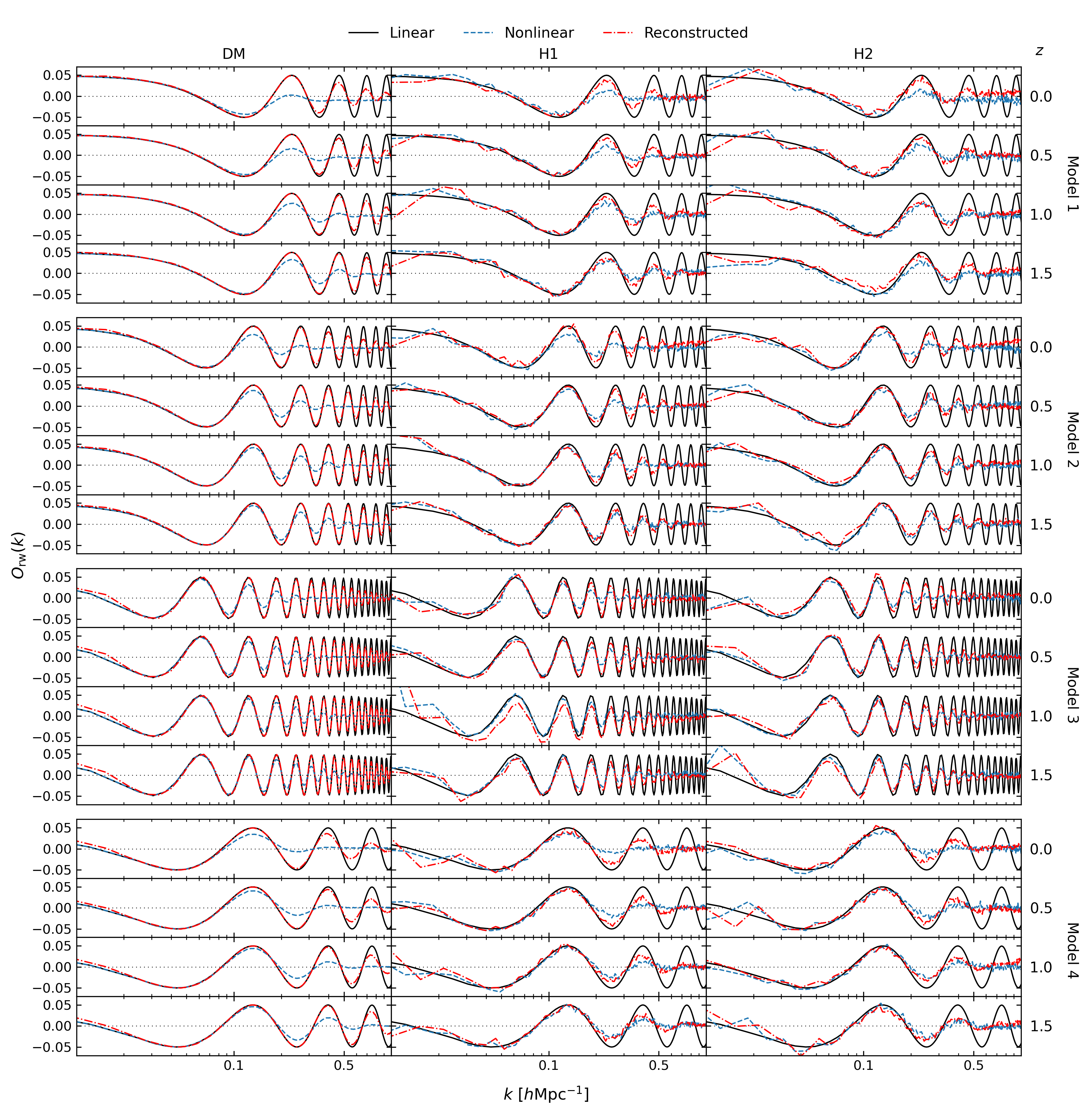
Figure 2: [Colour Online] Comparisons among the linear (black solid line), nonlinear (blue dash-dotted line) and reconstructed (red dashed line) $\textcolor{black}{O}_{\rm rw}$. The linear $\textcolor{black}{O}_{\rm rw}$ is measured from the initial conditions generated using 2LPTic, the nonlinear $\textcolor{black}{O}_{\rm rw}$ is measured from the output snapshots of the simulations, and the reconstructed $\textcolor{black}{O}_{\rm rw}$ is obtained from the reconstructed density field. Each row represents one redshift $z$ which is shown on the right side. The three columns denote, respectively, the results from the dark matter particle catalogue DM and the halo catalogues H1 and H2. Every four rows from the top down respectively belong to Model 1, Model 2, Model 3 blackand Model 4.

4 Results and discussion

In this section, we will first compare the linear, nonlinear and reconstructed $\textcolor{black}{O}_{\rm rw}$ measured for all models and redshifts. Then we present the results of the analytic fit to more quantitatively demonstrate the improvement by the reconstruction. Finally we show the results of the constraints on the oscillation parameters and give forecast for the DESI-like survey.

4.1 Comparisons among wiggle spectra

In Fig. 2, we compare the results of the linear, nonlinear and reconstructed $\textcolor{black}{O}_{\rm rw}(k)$ obtained from DM, H1 and H2 at the four redshifts for the blackfour wiggled models. The black solid lines represent the linear $\textcolor{black}{O}_{\rm rw}(k)$ obtained from the initial conditions of the simulations, which are equivalent to the primordial oscillatory features. The blue dashed lines represent the nonlinear $\textcolor{black}{O}_{\rm rw}(k)$ obtained from the output snapshots of the simulations, which are also referred to as the unreconstructed $\textcolor{black}{O}_{\rm rw}(k)$ for convenience. It can be seen that the wiggles on small scales are gradually damped as the redshift decreases. The red dash-dotted lines represent the reconstructed $\textcolor{black}{O}_{\rm rw}(k)$ obtained from the reconstructed density field, which helps to partially retrieve the damped wiggles.

The $\textcolor{black}{O}_{\rm rw}(k)$ results shown in the first column are obtained from DM, which exhibit some common characteristics for all three wiggled models. By comparing the unreconstructed results with the linear-theory predictions, it can be seen that the scale at which the wiggles start to be weakened becomes larger as time progresses. Furthermore, the wiggles on scales $k\gtrsim 0.3\ h\rm Mpc^{-1}$ are strongly damped at $z=0$, and so the recovery of the wiggles on scales $0.3\lesssim k\lesssim 0.5\ h\rm Mpc^{-1}$ would be an important objective of reconstruction. By comparing the reconstructed $\textcolor{black}{O}_{\rm rw}$ with the linear-theory prediction, we can see that, blackwhile the reconstructed power spectrum is not exactly the same as the linear spectrum, the reconstruction blackmethod to a certain extent helps retrieve the initial oscillations on our interested scales, $0.05\lesssim k\lesssim 0.5\ h\rm Mpc^{-1}$. blackThis agrees with the findings in Shi et al. (2018), which studied the performance of the same reconstruction method in dark matter reconstruction.

The success of the reconstruction from the dark matter particles is largely thanks to their high number density, which allows the late-time nonlinear density field to be accurately produced: in this sense, reconstruction from DM can be considered as an idealised case or an upper limit, which will be difficult to achieve in real observations. For a rough comparison, we have shown, in the middle and right columns of Fig. 2, the $\textcolor{black}{O}_{\rm rw}$ results obtained from the two halo catalogues, H1 and H2, which have number densities similar to typical real galaxy catalogues. These results are less impressive than those for the dark matter particles because of the much smaller halo number densities. Also due to the small halo number densities, these results are noisier, which in theory can be made smoother by having more realisations of simulations, or equivalently a larger volume.

By comparing the results of H1 and H2 for the same model, we find that there is no significant difference in the unreconstructed $\textcolor{black}{O}_{\rm rw}(k)$ at the same redshift, because the number densities of these two halo catalogues only differ by a factor of 2. In most cases the reconstructed $\textcolor{black}{O}_{\rm rw}$ results of H1 seem slightly better compared to those of H2, as a result of the slightly larger blackhalo number density in H1, though the difference is again insignificant visually. We shall revisit this point when discussing the analytical fit in the next subsection. Comparing the results with and without reconstruction, it is clear that the former does lead to less damped and sharper oscillation features, confirming that reconstruction can indeed help to partially blackretrieve the damped wiggles. This recovery seems more substantial at lower redshifts than at higher redshifts, since at higher redshifts there is blackless damping blackin the unreconstructed power spectra to start with. At lower redshifts, on the other hand, reconstruction can even recover some of the wiggles at $k\sim 0.5\ h\rm Mpc^{-1}$, where blackthe wiggles are strongly damped in the unreconstructed case. We expect that this will help blackto improve the accuracy of the measurements of wiggle parameters, especially in models with few wiggles at $k\lesssim 0.3\ h\rm Mpc^{-1}$ — we will discuss this in the parameter fittings next.

blackFinally, we notice that in rare cases, for example H1 at $z=1$ and H2 at $z=1.5$ for Model 3, the reconstructed $O_{\rm rw}$ seems to be poorer than the unreconstructed one. The exact cause of this is not clear, but we note that for these two cases the unreconstructed $O_{\rm rw}$ happens to be very noisy and deviate strongly from their theoretical values at large scales (a similar ’correlation’ can be observed in certain other panels across Fig. 2, though to a lesser extent). It is possible that the halo power spectra in these cases have inaccurate amplitudes of the oscillations on large scales, which affect the reconstruction results. Given that in both H1 and H2 this only affects a particular snapshot and not all snapshots, we suspect that it is related to the only one realisation per model we have used. Further investigation of this issue will be left for future works with more simulation realisations.

Table 2: The best-fit parameters of $\omega$, $\phi$ and $\zeta$ and their $95\%$ uncertainties for the four wiggled models studied in this work. blackThe values of $\omega$ and $\phi$ are respectively in the units of ${\rm Mpc}^{m}$ and $\pi$, and their theoretical values are shown below the title of each model on the top of the table. DM denotes the dark matter particle catalogue, H1 the halo catalogue with $n_{\rm halo}=1\times 10^{-3}(h^{-1}\rm Mpc)^{-3}$ and H2 the halo catalogue with $n_{\rm halo}=5\times 10^{-4}(h^{-1}\rm Mpc)^{-3}$. Each group of six rows includes the unreconstructed and reconstructed cases for the same redshift.

			Model 1			blueModel 2
			$\omega=40$, $\phi=0$			blue$\omega=70$, $\phi=0$
$z$		$\rm para$	$\rm DM$	$\rm H1$	$\rm H2$	blue$\rm DM$	blue$\rm H1$	blue$\rm H2$
$0.0$	unrec	$\omega$	$33.0\pm 3.4$	$36.5\pm 1.6$	$36.2\pm 1.9$	blue$68.5\pm 1.1$	blue$69.0\pm 1.7$	blue$68.4\pm 1.7$
		$\phi$	$0.09\pm 0.08$	$0.02\pm 0.04$	$0.04\pm 0.05$	blue$0.00\pm 0.03$	blue$0.01\pm 0.05$	blue$0.00\pm 0.04$
		$\zeta$	$7.23\pm 0.95$	$6.21\pm 0.44$	$6.90\pm 0.53$	blue$7.43\pm 0.26$	blue$6.95\pm 0.40$	blue$7.27\pm 0.41$
	rec	$\omega$	$40.0\pm 0.1$	$40.3\pm 0.4$	$40.8\pm 1.1$	blue$70.1\pm 0.1$	blue$70.1\pm 1.0$	blue$69.9\pm 0.9$
		$\phi$	$0.00\pm 0.01$	$-0.02\pm 0.02$	$-0.04\pm 0.04$	blue$-0.01\pm 0.01$	blue$0.00\pm 0.05$	blue$0.01\pm 0.04$
		$\zeta$	$2.05\pm 0.05$	$3.41\pm 0.13$	$4.07\pm 0.32$	blue$2.06\pm 0.03$	blue$3.58\pm 0.28$	blue$4.00\pm 0.25$
$0.5$	unrec	$\omega$	$37.6\pm 1.4$	$37.3\pm 1.1$	$37.7\pm 1.0$	blue$69.1\pm 0.4$	blue$68.0\pm 0.9$	blue$68.2\pm 1.2$
		$\phi$	$0.02\pm 0.04$	$0.03\pm 0.03$	$0.02\pm 0.03$	blue$0.00\pm 0.01$	blue$0.05\pm 0.03$	blue$0.02\pm 0.04$
		$\zeta$	$5.53\pm 0.40$	$5.27\pm 0.32$	$5.71\pm 0.29$	blue$5.88\pm 0.10$	blue$5.72\pm 0.23$	blue$6.18\pm 0.30$
	rec	$\omega$	$40.0\pm 0.1$	$40.1\pm 0.3$	$40.3\pm 0.7$	blue$70.1\pm 0.1$	blue$70.1\pm 0.4$	blue$69.7\pm 0.6$
		$\phi$	$0.00\pm 0.01$	$-0.01\pm 0.02$	$-0.01\pm 0.03$	blue$-0.01\pm 0.01$	blue$0.00\pm 0.02$	blue$0.01\pm 0.03$
		$\zeta$	$1.52\pm 0.04$	$3.17\pm 0.10$	$3.75\pm 0.20$	blue$1.51\pm 0.04$	blue$3.12\pm 0.10$	blue$3.83\pm 0.17$
$1.0$	unrec	$\omega$	$38.6\pm 0.6$	$38.0\pm 0.7$	$37.5\pm 0.9$	blue$69.5\pm 0.2$	blue$68.7\pm 0.8$	blue$69.0\pm 0.8$
		$\phi$	$0.01\pm 0.02$	$0.01\pm 0.03$	$0.01\pm 0.03$	blue$0.00\pm 0.01$	blue$0.02\pm 0.03$	blue$0.00\pm 0.03$
		$\zeta$	$4.39\pm 0.18$	$4.38\pm 0.22$	$5.08\pm 0.26$	blue$4.73\pm 0.05$	blue$4.90\pm 0.21$	blue$5.48\pm 0.20$
	rec	$\omega$	$40.0\pm 0.1$	$40.1\pm 0.3$	$39.7\pm 0.7$	blue$70.0\pm 0.1$	blue$70.0\pm 0.5$	blue$70.0\pm 0.7$
		$\phi$	$0.00\pm 0.01$	$-0.01\pm 0.02$	$0.01\pm 0.03$	blue$0.00\pm 0.01$	blue$0.00\pm 0.02$	blue$-0.01\pm 0.03$
		$\zeta$	$1.09\pm 0.04$	$3.09\pm 0.11$	$3.56\pm 0.20$	blue$1.11\pm 0.03$	blue$3.23\pm 0.14$	blue$3.81\pm 0.20$
$1.5$	unrec	$\omega$	$39.3\pm 0.3$	$38.1\pm 0.7$	$36.5\pm 0.8$	blue$69.6\pm 0.1$	blue$69.1\pm 0.8$	blue$68.2\pm 1.0$
		$\phi$	$0.00\pm 0.01$	$0.02\pm 0.03$	$0.07\pm 0.03$	blue$0.00\pm 0.01$	blue$0.01\pm 0.03$	blue$0.03\pm 0.03$
		$\zeta$	$3.60\pm 0.10$	$4.07\pm 0.20$	$4.92\pm 0.25$	blue$3.90\pm 0.02$	blue$4.43\pm 0.21$	blue$5.17\pm 0.26$
	rec	$\omega$	$40.0\pm 0.1$	$39.6\pm 0.5$	$40.1\pm 1.1$	blue$70.0\pm 0.1$	blue$70.2\pm 0.4$	blue$69.6\pm 1.1$
		$\phi$	$0.00\pm 0.01$	$0.02\pm 0.02$	$-0.01\pm 0.05$	blue$0.00\pm 0.01$	blue$-0.01\pm 0.02$	blue$0.01\pm 0.05$
		$\zeta$	$0.84\pm 0.03$	$3.08\pm 0.15$	$3.66\pm 0.32$	blue$0.88\pm 0.03$	blue$3.24\pm 0.12$	blue$3.90\pm 0.29$
			Model 3			blueModel 4
			$\omega=150$, $\phi=0$			blue$\omega=28.9$, $\phi=0$
$z$		$\rm para$	$\rm DM$	$\rm H1$	$\rm H2$	blue$\rm DM$	blue$\rm H1$	blue$\rm H2$
$0.0$	unrec	$\omega$	$149.3\pm 0.4$	$151.2\pm 2.0$	$151.6\pm 2.1$	blue$26.1\pm 0.6$	blue$27.2\pm 1.0$	blue$25.9\pm 1.0$
		$\phi$	$0.01\pm 0.01$	$-0.04\pm 0.05$	$-0.05\pm 0.04$	blue$0.11\pm 0.04$	blue$0.06\pm 0.06$	blue$0.14\pm 0.06$
		$\zeta$	$7.95\pm 0.09$	$7.44\pm 0.51$	$8.51\pm 0.50$	blue$6.96\pm 0.23$	blue$6.62\pm 0.35$	blue$6.68\pm 0.36$
	rec	$\omega$	$150.1\pm 0.1$	$150.7\pm 0.6$	$150.7\pm 1.0$	blue$29.0\pm 0.1$	blue$29.5\pm 0.4$	blue$28.7\pm 0.6$
		$\phi$	$-0.01\pm 0.01$	$-0.04\pm 0.03$	$-0.03\pm 0.04$	blue$-0.01\pm 0.01$	blue$-0.05\pm 0.03$	blue$0.03\pm 0.05$
		$\zeta$	$2.13\pm 0.04$	$3.70\pm 0.19$	$4.04\pm 0.28$	blue$2.11\pm 0.04$	blue$3.41\pm 0.14$	blue$3.75\pm 0.22$
$0.5$	unrec	$\omega$	$149.6\pm 0.2$	$150.4\pm 0.9$	$150.4\pm 1.5$	blue$27.2\pm 0.2$	blue$27.2\pm 0.6$	blue$26.2\pm 0.7$
		$\phi$	$0.01\pm 0.01$	$-0.01\pm 0.02$	$-0.02\pm 0.03$	blue$0.07\pm 0.02$	blue$0.06\pm 0.05$	blue$0.12\pm 0.05$
		$\zeta$	$6.30\pm 0.05$	$6.02\pm 0.23$	$6.85\pm 0.39$	blue$5.33\pm 0.08$	blue$4.96\pm 0.23$	blue$5.58\pm 0.26$
	rec	$\omega$	$150.1\pm 0.1$	$150.0\pm 0.5$	$150.1\pm 0.8$	blue$29.0\pm 0.1$	blue$29.1\pm 0.3$	blue$29.3\pm 0.4$
		$\phi$	$-0.01\pm 0.01$	$-0.01\pm 0.02$	$-0.02\pm 0.03$	blue$-0.01\pm 0.01$	blue$-0.03\pm 0.03$	blue$-0.03\pm 0.04$
		$\zeta$	$1.63\pm 0.03$	$3.37\pm 0.15$	$3.96\pm 0.23$	blue$1.53\pm 0.04$	blue$3.04\pm 0.11$	blue$3.46\pm 0.16$
$1.0$	unrec	$\omega$	$149.7\pm 0.1$	$149.9\pm 0.9$	$149.3\pm 0.9$	blue$27.7\pm 0.1$	blue$27.1\pm 0.5$	blue$26.7\pm 0.5$
		$\phi$	$0.01\pm 0.01$	$0.00\pm 0.03$	$0.02\pm 0.03$	blue$0.05\pm 0.01$	blue$0.08\pm 0.04$	blue$0.10\pm 0.03$
		$\zeta$	$5.08\pm 0.03$	$5.29\pm 0.25$	$5.95\pm 0.24$	blue$4.19\pm 0.03$	blue$4.30\pm 0.20$	blue$4.99\pm 0.17$
	rec	$\omega$	$150.1\pm 0.1$	$150.6\pm 1.7$	$149.9\pm 0.6$	blue$29.0\pm 0.1$	blue$28.7\pm 0.4$	blue$28.3\pm 0.4$
		$\phi$	$-0.01\pm 0.01$	$-0.04\pm 0.08$	$0.00\pm 0.03$	blue$-0.01\pm 0.01$	blue$0.02\pm 0.03$	blue$0.04\pm 0.04$
		$\zeta$	$1.27\pm 0.03$	$3.31\pm 0.52$	$3.85\pm 0.17$	blue$1.12\pm 0.03$	blue$3.04\pm 0.13$	blue$3.55\pm 0.15$
$1.5$	unrec	$\omega$	$149.7\pm 0.1$	$149.6\pm 0.8$	$149.6\pm 0.9$	blue$28.0\pm 0.1$	blue$27.4\pm 0.6$	blue$27.0\pm 0.6$
		$\phi$	$0.01\pm 0.01$	$0.01\pm 0.03$	$0.01\pm 0.03$	blue$0.04\pm 0.01$	blue$0.05\pm 0.05$	blue$0.08\pm 0.04$
		$\zeta$	$4.21\pm 0.02$	$4.88\pm 0.23$	$5.71\pm 0.24$	blue$3.41\pm 0.02$	blue$3.92\pm 0.22$	blue$4.73\pm 0.21$
	rec	$\omega$	$150.1\pm 0.1$	$150.0\pm 0.7$	$150.0\pm 1.2$	blue$28.9\pm 0.1$	blue$29.0\pm 0.4$	blue$28.9\pm 0.5$
		$\phi$	$-0.01\pm 0.01$	$-0.01\pm 0.03$	$0.00\pm 0.05$	blue$0.00\pm 0.01$	blue$-0.02\pm 0.04$	blue$-0.01\pm 0.04$
		$\zeta$	$1.07\pm 0.03$	$3.38\pm 0.20$	$4.07\pm 0.34$	blue$0.83\pm 0.02$	blue$3.19\pm 0.16$	blue$3.65\pm 0.17$

Table 3: blackThe ratios of unreconstructed to reconstructed $\zeta$, black$\zeta_{\rm unrec}/\zeta_{\rm rec}$, obtained from Table 2, which can be used to describe the reconstruction efficiency, in all cases blackconsidered in Table 2.

	Model 1			blueModel 2			Model 3			blueModel 4
$z$	$\rm DM$	$\rm H1$	$\rm H2$	blue$\rm DM$	blue$\rm H1$	blue$\rm H2$	$\rm DM$	$\rm H1$	$\rm H2$	blue$\rm DM$	blue$\rm H1$	blue$\rm H2$
$0.0$	$3.52$	$1.82$	$1.69$	blue$3.61$	blue$1.94$	blue$1.82$	$3.73$	$2.01$	$2.11$	blue$3.30$	blue$1.94$	blue$1.78$
$0.5$	$3.64$	$1.66$	$1.52$	blue$3.89$	blue$1.83$	blue$1.61$	$3.87$	$1.79$	$1.73$	blue$3.48$	blue$1.63$	blue$1.61$
$1.0$	$4.03$	$1.42$	$1.43$	blue$4.26$	blue$1.52$	blue$1.44$	$4.00$	$1.60$	$1.54$	blue$3.74$	blue$1.41$	blue$1.41$
$1.5$	$4.29$	$1.32$	$1.34$	blue$4.43$	blue$1.37$	blue$1.33$	$3.93$	$1.44$	$1.40$	blue$4.11$	blue$1.23$	blue$1.30$

4.2 Wiggle parameter fitting

The corresponding best-fit parameters of $\omega$, $\phi$ and $\zeta(z)$, as well as their uncertainties, are given in Table 2, which assist the understanding from a quantitative perspective. blackThe relevant figures showing the analytic fit to the data can be found in the Appendix. As mentioned before, we will mainly focus on the results of H1 and H2, and so the results of DM would be taken as a reference and not be discussed in detail. The three parameters are mainly determined by the remaining peaks in the wiggles. We shall first discuss the results of the damping parameter, followed by the oscillation parameters, and then combine them to clarify the improvement given by reconstruction.

The damping parameter $\zeta$ effectively describes the extent of the blackdamping effects blackcaused by the gravitational nonlinearities and characterises the suppression of the primordial oscillations. It is zero in the linear regime, such as at blackthe initial redshift $z=49$, and gradually increases blackat lower redshifts as the structures become progressively more nonlinear blackand consequently more information of the wiggles in the primordial power spectrum gets blackdamped. Thus reconstruction has the aim to reduce $\zeta$ and retrieve the primordial oscillations. Table 2 shows that the reconstructed values of $\zeta$ are evidently smaller than the unreconstructed values in all cases. Apart from a few high-redshift ($z>1$) cases, the uncertainties of most cases are also reduced after reconstruction, which confirms that the reconstruction blacksuccessfully retrieves the damped wiggles to blackan appreciable extent. Specifically, by comparing the cases among different models but the same catalogues and redshifts, the corresponding values after reconstruction seem to be nearly independent of the model, which implies that the improvement on the recovery of the wiggles does not blackstrongly depend on the shape of the primordial oscillations.

blackblackFor a closer inspection, we show the ratios of unreconstructed to reconstructed $\zeta$ in Table 3, black$\zeta_{\rm unrec}/\zeta_{\rm rec}$, which can be considered as an indicator of the reconstruction efficiency. We do this for all the cases black(models, tracer types and redshifts) listed in Table 2. The blackreconstruction efficiency of halo catalogues H1 and H2 increases with decreasing redshift, which shows that reconstruction is more beneficial for lower redshifts ($z<1$). blackThis is to be expected, given that the halo density field is more nonlinear at low $z$ and so the unreconstructed $\zeta$ is significantly larger than at high $z$; on the other hand, the reconstructed $\zeta$ depends more mildly on $z$, so that the ratio black$\zeta_{\rm unrec}/\zeta_{\rm rec}$ increases with decreasing $z$. Also, among the low-redshift ($z<1$) cases, the larger number density of H1 leads to higher efficiency when compared blackwith H2 at the same redshift. For the DM case, the trend is reversed, with the ratio between unreconstructed and reconstructed $\zeta$ values increasing with redshift. Here the behaviour is quite different from the halo cases, with the reconstructed $\zeta$ decreasing much faster with increasing redshift $z$. blackWe have checked (though not shown here) that the values of $\zeta_{\rm unrec}/\zeta_{\rm rec}$ for the primordial features studied here are broadly consistent with the reconstruction efficiency defined in the same way applied to the reconstruction of BAO wiggles in Birkin et al. (2019, which uses the same reconstruction method and similar tracer number density).

Next, let us consider whether the black‘sharpened’ wiggles after reconstruction can lead to more accurate measurements of the oscillation parameters $\omega$ and $\phi$. Regarding the oscillation frequency $\omega$, the reconstructed values of $\omega$ are much closer to the theoretical values than the unreconstructed values in all cases, which is especially evident at low redshifts. Except for a few high-redshift cases, the improvement on the uncertainties after reconstruction is evident in most cases as well. blackThe unreconstructed $\omega$ values of Model 2 and Model 3 appear to be closer to their theoretical values than in Model 1 and Model 4, which is probably because the former two models have more oscillation periods within the fitting range of scales than the latter two (see the right panel of Fig. 1, or the blue lines in Fig. 2). After reconstruction, however, there is less clear difference among the four models, either in how close the reconstructed $\omega$ is to the theoretical value or in their uncertainties. Likewise, the difference between the best-fit reconstructed $\omega$ values in H1 and H2 is rather mild, although the uncertainties are generally smaller for the former catalogue. blackOverall, the results indicate that reconstruction does indeed lead to a stronger improvement of the measurement of $\omega$ in Models 1 and 4, which have fewer visible peaks at $k\lesssim 0.5h\mathrm{Mpc}^{-1}$.

The situation is quite different in the case of the oscillation phase $\phi$. blackThe unreconstructed values of $\phi$ in Model 1, Model 2 and Model 3 are determined very well in most cases, so the reconstructed values only show a little improvement on the unreconstructed $\phi$ even for low-redshift cases. However, for Model 4 the unreconstructed values largely deviate from the theoretical value in all cases, and the unreconstructed values of H2 deviate even further than those of H1 at the same redshift. Although we can not exclude the possibility that this discrepancy is an effect caused by the particular simulation, since we have only one realisation for each model, we doubt this would be the cause, because the same random phases have been used to generate the ICs for all simulations. Instead, we suspect that this is more likely to be caused by the fact that $m\neq 1$ in blackModel 4, which means that the oscillation pattern is more complicated and thus leads to a less accurate fitting of $\phi$. Regardless, based on the table, it seems that the reconstruction once again enables more accurate measurement of $\phi$, especially for H2 at low redshift.

blackWhen considering the results of all three parameters, it seems that the reconstruction is most useful at low redshifts, $z<1$, and Model 1 and Model 4 benefit more from it than Model 2 and Model 3 do. Although the peaks of Model 2 and Model 3 are better preserved after the cosmic evolution so that their reconstructed results are better than those of the other two models, the improvement is relatively limited, suggesting that the improvement depends not only on how clear-cut the reconstructed wiggles are, but also on how poorly the primordial wiggles are preserved before reconstruction. Overall, reconstruction seems more useful where the primordial wiggles are more damped. As we mentioned before, the wiggles on scales $k\gtrsim 0.3\ h\rm Mpc^{-1}$ are strongly damped at $z=0$; Model 2 and Model 3 have exactly the first several original peaks outside this range of scales, so these peaks are effectively preserved at low redshift. By contrast, we designed Model 4 so that it has one original peak at the same position of the first peak of Model 2 which is effectively preserved, and its second peak is at the same position of the third peak of Model 2, which is strongly damped. Therefore, the primordial wiggles of Model 4 are preserved less well than those of Model 2, and this Model benefits more from the reconstruction. Similarly, Model 1 has two original peaks in the range $k\lesssim 0.5\ h\rm Mpc^{-1}$: the first is at a smaller scale compared with the first peak of the other models and thus is not preserved as well as the first peak of the other models due to the stronger damping effect, while the second peak is completely damped. Therefore Model 1 and Model 4 both benefit from the reconstruction substantially more than Model 2 and Model 3.

Additionally, the values of $\omega$ used in Model 1, Model 2 and Model 3 imply that the reconstruction method is not only effective at low frequency, such as $\sim 40\ \rm Mpc$, but also working well at relatively higher frequency, such as $\sim 150\ \rm Mpc$.

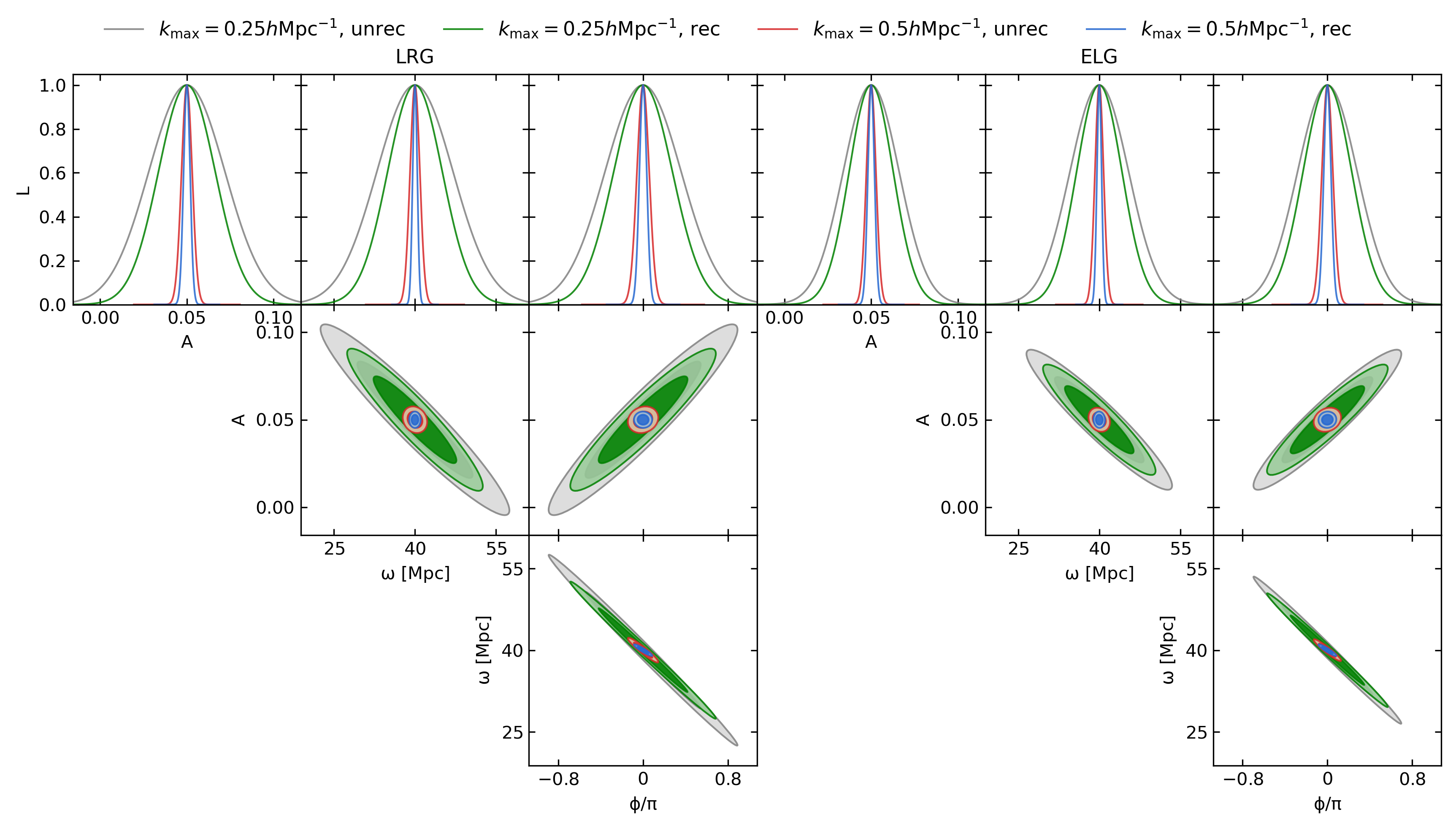
Figure 3: [Colour Online] Forecasts of constraints on the oscillatory feature parameters for a DESI-like survey with a survey area of $14,000$ $\rm deg^{2}$, for the primordial oscillations of Model 1. The left side is for LRGs and the right side is for ELGs. The upper panels show the 1D marginalised blackposterior distributions. The middle and lower panels show the marginalised $68\%$ and $95\%$ confidence contours for every two out of three feature parameters. The green and grey colours represent, respectively, the cases for $k_{\rm max}=0.25h\rm Mpc^{-1}$ with and without reconstruction, while the blue and red colours represent the cases for $k_{\rm max}=0.5h\rm Mpc^{-1}$ with and without reconstruction.

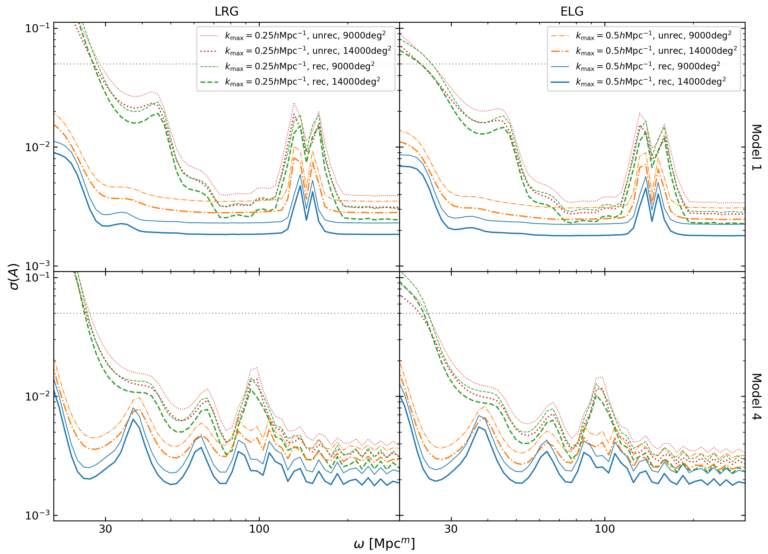
Figure 4: [Colour Online] Forecasts of the marginalised uncertainties of the oscillation amplitude $A$ as a function of the frequency $\omega$, for the blacktwo models, blackModel 1 (top row) and blackModel 4 (bottom row); the result for Model 2 and Model 3 are not shown here since the two models have the identical form of oscillations to that of Model 1. The first column is for LRGs and the second column is for ELGs. The dotted black lines mark the theoretical amplitudes of the oscillations, $A=0.05$, used in the forecasts. The meanings of the different colours and line styles are indicated in the legends. The same colours represent the cases with same $k_{\rm max}$ and same situation of reconstruction but different survey areas; the thick lines are for the survey area of $14,000$ $\rm deg^{2}$ and the thin lines are for $9,000$ $\rm deg^{2}$.

4.3 Constraints on oscillation parameters for DESI-like survey

blackSince the four wiggled models have similar results of the constraints on the oscillation parameters, we shall take Model 1 as an example to illustrate and discuss how the reconstruction potentially improves the constraints in a real galaxy survey. Additionally, we also forecast how much the uncertainties of the feature amplitude can be reduced after reconstruction for the wiggled models.

blackFig. 3 shows the forecasted constraints on the oscillation parameters for a DESI-like survey with a survey area of 14,000 $\rm deg^{2}$, based on the primordial oscillations of Model 1. The marginalised posterior distribution of each parameter shown in the upper panels indicates that, without reconstruction, the case of $k_{\rm max}=0.5\ h\rm Mpc^{-1}$ (the red lines) give better constraints than the case with $k_{\rm max}=0.25\ h\rm Mpc^{-1}$ (grey), because in the former case more $k$ modes are included in the Fisher matrix and increase the accuracy of the constraints. Additionally, by comparing the cases with the same $k_{\rm max}$ (red versus blue, or grey versus green lines), we find that reconstruction leads to stronger constraints on the parameters, especially with $k_{\rm max}=0.5\ h\rm Mpc^{-1}$. This is because the oscillation wiggles on scales $k\gtrsim 0.25\ h\rm Mpc^{-1}$ are heavily damped at low redshift without any reconstruction, while the reconstructed wiggles at $k=(0.25-0.5)\ h\rm Mpc^{-1}$ significantly contribute to the constraints. By contrast, since the peaks on scales $k\lesssim 0.25\ h\rm Mpc^{-1}$ are preserved reasonably well, the reconstruction for $k_{\rm max}=0.25\ h\rm Mpc^{-1}$ does not lead to as much benefit as in the case of $k_{\rm max}=0.5\ h\rm Mpc^{-1}$. Furthermore, stronger constraints are shown for ELGs (right panels) compared with LRGs (left panels), because the former has more available redshift bins and larger number density for the same redshift bins.

blackIn particular, every two out of three parameters show degeneracies in the confidence contours when $k_{\rm max}=0.25\ h\rm Mpc^{-1}$, though these degeneracies are broken and replaced with stronger constraints when $k_{\rm max}=0.5\ h\rm Mpc^{-1}$ in the $A$–$\omega$ and $A$–$\phi$ contours due to more $k$ modes included. By contrast, the $\omega$–$\phi$ contours keep the degeneracy which is a consequence caused by the oscillation model itself and by the fact that here we are trying to constrain both oscillatory frequency and phase over a limited range of $k$.

Lastly, similar to previous works (Slosar et al., 2019; Beutler et al., 2019; Ballardini et al., 2020), we show the marginalised uncertainties of feature amplitude as a function of oscillatory frequency for our feature models in Fig. 4 and discuss the implications of the results. Because Model 1, Model 2 and Model 3 have an identical form of oscillations and almost same damping parameters within the error bars, we only show the results of Model 1 and blackModel 4 here.

We consider Model 1 first. As expected, ELGs place slightly tighter constraints than LRGs due to their larger number densities and redshift range. The sharp peaks that appear at black$\omega\simeq 150\ {\rm Mpc}$ are due to the degeneracy between the oscillatory features and the BAO wiggles. blackWe have tested that for $\omega\gtrsim 200\ {\rm Mpc}$ the uncertainties almost stay as a constant, and so we have cut off the figure at $\omega^{m}=300\ {\rm Mpc}^{m}$. For smaller $\omega$, things are complicated and behave differently for different $k_{\rm max}$. For $k_{\rm max}=0.25\ h\rm Mpc^{-1}$ we can see an increase in the uncertainties at black$\omega\lesssim 70\ {\rm Mpc}$, while a similar increase starts to appear at even smaller black$\omega$ – $30\ {\rm Mpc}$ – for $k_{\rm max}=0.5\ h\rm Mpc^{-1}$. Thus larger $k_{\rm max}$ has an extra advantage of significantly reducing the uncertainties for small $\omega$, in addition to giving more stringent constraints (everything else the same) for all $\omega$ overall. By comparing the pairs of curves with the same colours, i.e., the same cases ($k_{\rm max}$ and reconstructed vs. unreconstructed) but different survey areas, we find that, as expected, a larger survey area always gives better constraints.

Most interestingly, everything else equal, performing blackthe nonlinear reconstruction can significantly reduce the uncertainties of $A$. As an example, for large values of $\omega$, in the case of $k_{\rm max}=0.5\ h\rm Mpc^{-1}$ and a survey area equal to $14,000~{}{\rm deg}^{2}$, reconstruction reduces $\sigma(A)$ from $\sim 0.003$ to $\sim 0.002$, and this improvement is stronger than not performing reconstruction, but instead going from $9,000$ to $14,000$ ${\rm deg}^{2}$ with $k_{\rm max}$ fixed to $0.25$ or $0.5\ h\rm Mpc^{-1}$, or increasing $k_{\rm max}$ from $0.25$ to $0.5\ h\rm Mpc^{-1}$ keeping the survey area fixed to either $9,000$ or $14,000$ ${\rm deg}^{2}$. A similarly good improvement can be seen with $k_{\rm max}=0.25\ h\rm Mpc^{-1}$ or survey area equal to $9,000$ ${\rm deg}^{2}$, when doing reconstruction. In certain cases, e.g., the large-$\omega$ regime of the lower panels of Fig. 4, reconstruction with $k_{\rm max}=0.25\ h\rm Mpc^{-1}$ and a survey area equal to $9,000$ ${\rm deg}^{2}$ (the thin green dashed line) can lead to comparable constraints to not doing reconstruction but with $k_{\rm max}=0.5\ h\rm Mpc^{-1}$ and a survey area equal to $14,000$ ${\rm deg}^{2}$ (the thick orange dot-dashed line). blackGiven that increasing survey area is not always possible due to the finite sky area, but increasing $k_{\rm max}$ in analyses for these primordial feature models is comparably blackmore straightforward (Beutler et al., 2019), combining an increase in $k_{\rm max}$ with blacknonlinear reconstruction can blackbe a potentially promising way to obtain even stronger constraints on the feature parameters, and help to maximise the scientific return of future survey data.

The behaviour of blackModel 4 is similar to that of Model 1, e.g., both the absolute and the relative heights of the different curves, as well as their shapes are the same as before. There are, however, some notable differences, e.g., the main peaks in $\sigma(A)$ in blackModel 4 are at slightly different values of $\omega$ from the other models, and the curves are also less smooth. As mentioned above, the bump (which has the structure of a double peak) of $\sigma(A)$ for Model 1 is related to the BAO peak in the matter/galaxy correlation function, which is at black$\simeq 150\ {\rm Mpc}$. The primordial wiggles of Model 1, in configuration space, correspond to a spike at matter or halo separation $r=\omega$. When black$\omega\gg 150\ {\rm Mpc}$, the BAO and primordial peaks are separated afar and thus the former does not affect the accuracy of the measurement for the latter. As $\omega$ approaches black$150\ {\rm Mpc}$ from above, the BAO and primordial peaks start to ‘interfere’, leading to changes of both the amplitude and shape of the latter, making it harder to measure its parameters accurately. We speculate that the dip — which causes the double-peak structure in $\sigma(A)$ for Model 1 — is due to the fact that, when the primordial peak does not coincide well with the centre of the (rather wide) BAO peak, its shape can be affected in an asymmetric manner, making the measurement of its parameters even more inaccurate. In contrast, the structure of the primordial wiggles in blackModel 4 is more complicated in configuration space, because $m\neq 1$ in Eq. (2), which can cause the differences in the blackunits of $\omega$ and other fine details of $\sigma(A)$ between this and the other models.

5 Conclusions

In this paper, we have investigated the effect of blacka nonlinear density reconstruction method on retrieving hypothetical oscillatory features in the primordial power spectrum which are blacksignificantly damped on small scales in the late-time Universe due to cosmological blackstructure formation.

We considered blackfour different oscillatory features which are added to a simple power-law type primordial power spectrum, for which we ran N-body simulations and identified dark matter halo catalogues at a number of redshifts. We reconstructed the initial density fields from the particle data and halo catalogues with two different number densities. Finally, we compared the fitted feature parameters from blackthe power spectra of the unreconstructed and reconstructed density fields, to identify the improvement by reconstruction. We showed that blacknonlinear reconstruction blackcan effectively help to retrieve the damped wiggles blackwith a range of frequencies between $40\ \rm Mpc$ and $150\ \rm Mpc$ — not only does it lead to less biased best-fit values of the feature parameters, but it also substantially shrinks the measurement uncertainty. The improvement was especially strong where the primordial features have been blackless well preserved pre-reconstruction to start with, such as at $z<1$.

In order to forecast the constraints on the feature parameters from a DESI-like galaxy survey, we modelled the observed broadband galaxy power spectrum based on the halofit blackprediction of the nonlinear matter power spectrum with the addition of oscillatory features blackstudied in this work, and then used the analytic marginalised Fisher matrix to calculate the blackexpected constraints on the oscillation parameters blackusing the specifications of DESI LRGs and ELGs. We found that blacknonlinear reconstruction led to more robust constraints on the oscillation parameters, with the equivalent effects of enlarging the survey area (but at a much smaller cost) and/or increasing the $k$ range.

While blacknonlinear reconstruction blackhas been proposed to be used in improving the measurement of the BAO scale (e.g., Wang et al., 2017), and hence the determination of the expansion rate blackof the Universe and blackhence the properties of dark energy, this work has demonstrated that similar applications are possible in other cases where certain features in matter clustering are presentblack, following the spirit of earlier works such as Beutler et al. (2019). This is particularly true if these features are in the mildly nonlinear regime, $0.1\lesssim{k/(h{\rm Mpc}^{-1})}\lesssim 0.5$, since this range of scales is what the nonlinear reconstruction method used here helps most: on even larger scales the benefit of reconstruction is insignificant, while on further smaller scales reconstruction will not help much.

The methodology exemplified in this paper assumes that we know the functional form of the primordial features a priori — this is how we forecasted constraints on the oscillation amplitude $A$. However, the reconstruction step is completely independent of any assumption of a particular primordial feature, and hence any method developed for detecting general features from the matter clustering should apply to and benefit from the reconstructed density field.

As a first step, the present study is based on various simplifications, and we discuss a couple here which can be improved in the future. The first is related to the post-reconstruction damping parameter $\zeta$. As we have discussed, $\zeta$ characterises the damping of the primordial features, and a smaller $\zeta$ means that the reconstruction has done a better job. blackDue to the limited number of simulations carried out in this work (one realisation per model), shot noise will impact the estimated reconstruction efficiency. This could be improved by increasing the number of simulations and more studies are needed in the future.

The second is related to the modelling of redshift-space distortions (RSD), for which we have adopted a simplistic prescription and well pushed beyond the limit (e.g., $k\simeq 0.5~{}h{\rm Mpc}^{-1}$) where it is expected to work. This is not an issue for a forecast work, but for constraints using real data it should be treated more carefully. The reconstruction method here has been extended to remove RSD from observed galaxy catalogues (Wang et al., 2020), though that is unlikely to work reliably at $k$ as large as $\simeq 0.5~{}h{\rm Mpc}^{-1}$. Of course, we can always cut $k_{\rm max}$ to something that we are comfortable with. However, as mentioned above, if we would like to take maximum benefit from reconstruction, it is likely that we need to go substantially beyond $k\simeq 0.1~{}h{\rm Mpc}^{-1}$. This can be achieved, for example, by using emulators of redshift-space galaxy or halo clustering (see, e.g., Zhai et al., 2019; Kobayashi et al., 2020); actually, as long as the primordial oscillations are weak (as implied by current null detections), one might assume that their presence has little or negligible impact on RSD.

The ultimate objective, of course, is to apply this method to real observation data from future galaxy surveys such as Euclid and DESI. For this, the above-mentioned improvements, amongst many others, would need to be done properly. These will be left for future works, in which we plan to carry out updated forecasts for these surveys and eventually real constraints.

Data Availability

Simulation data used in this work can be made available upon request to the authors.

Appendix A Results of wiggle fitting

Figs. 5, 6, 7 and 8 show, respectively, the results of the analytic fit to the unreconstructed and reconstructed $\textcolor{black}{O}_{\rm rw}$ results for the blackfour models studied in this work. It can be seen that, in most cases, the analytic model Eq. (5), with a Gaussian damping function characterised by the parameter $\zeta(z)$, fits the pre- and post-reconstruction data very well.

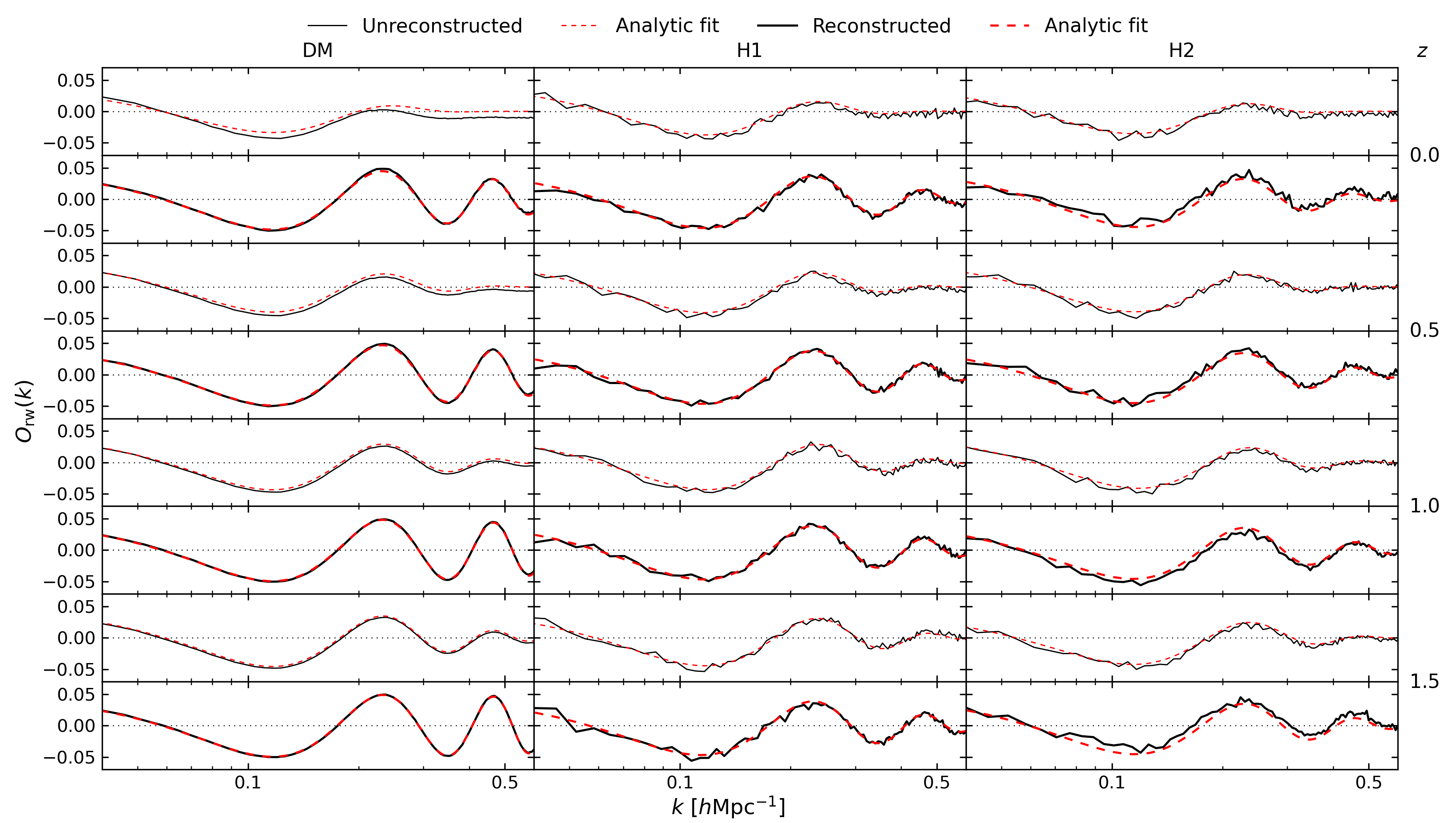
Figure 5: [Colour Online] The analytic fit to the unreconstructed and reconstructed $\textcolor{black}{O}_{\rm rw}$ for Model 1. The black solid lines represent the measured $\textcolor{black}{O}_{\rm rw}$ and the red dashed lines represent the fitting curves given by the analytic model, Eq. (5). The thin lines are for the unreconstructed cases and the thick lines are for the reconstructed cases. The three columns from left to right respectively denote the dark matter particle catalogue DM, and the halo catalogues H1 and H2. Every two rows from the top down represent the same redshift shown on the right side. In each group of two rows, the upper one is for the unreconstructed, and the lower one for the reconstructed, case.

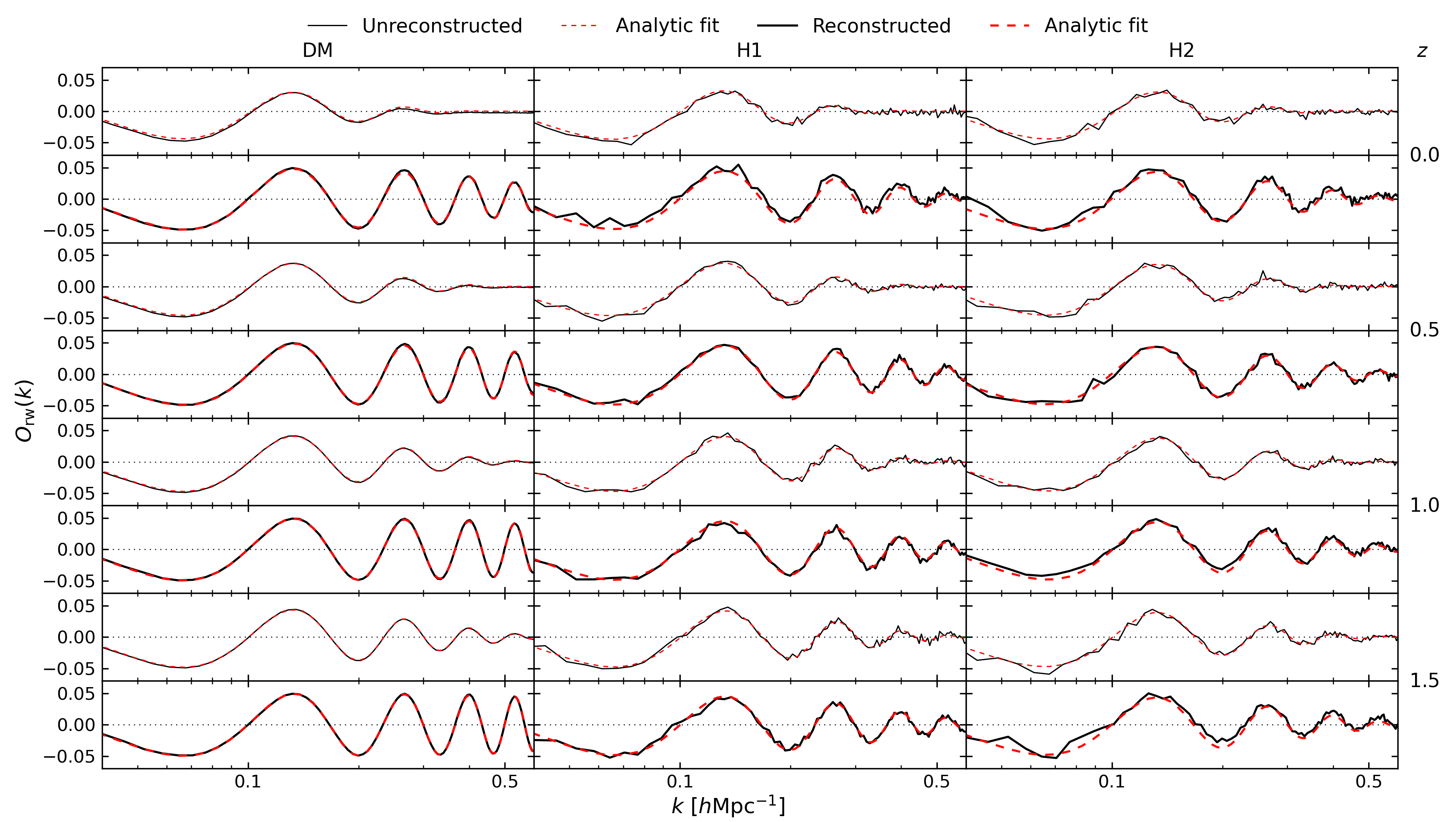
Figure 6: [Colour Online] The same as Fig. 5 but for Model 2.

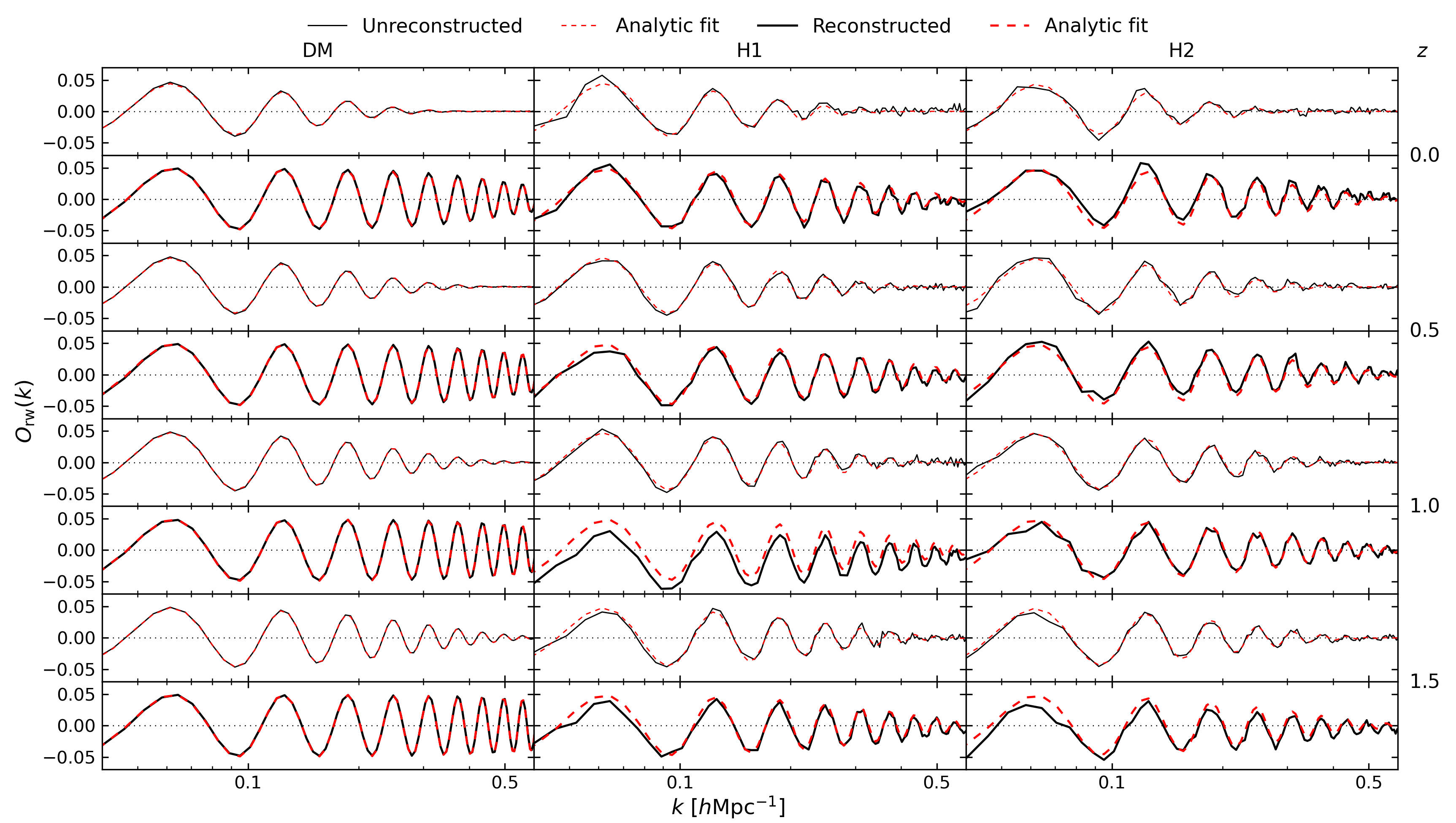
Figure 7: [Colour Online] The same as Fig. 5 but for Model 3.

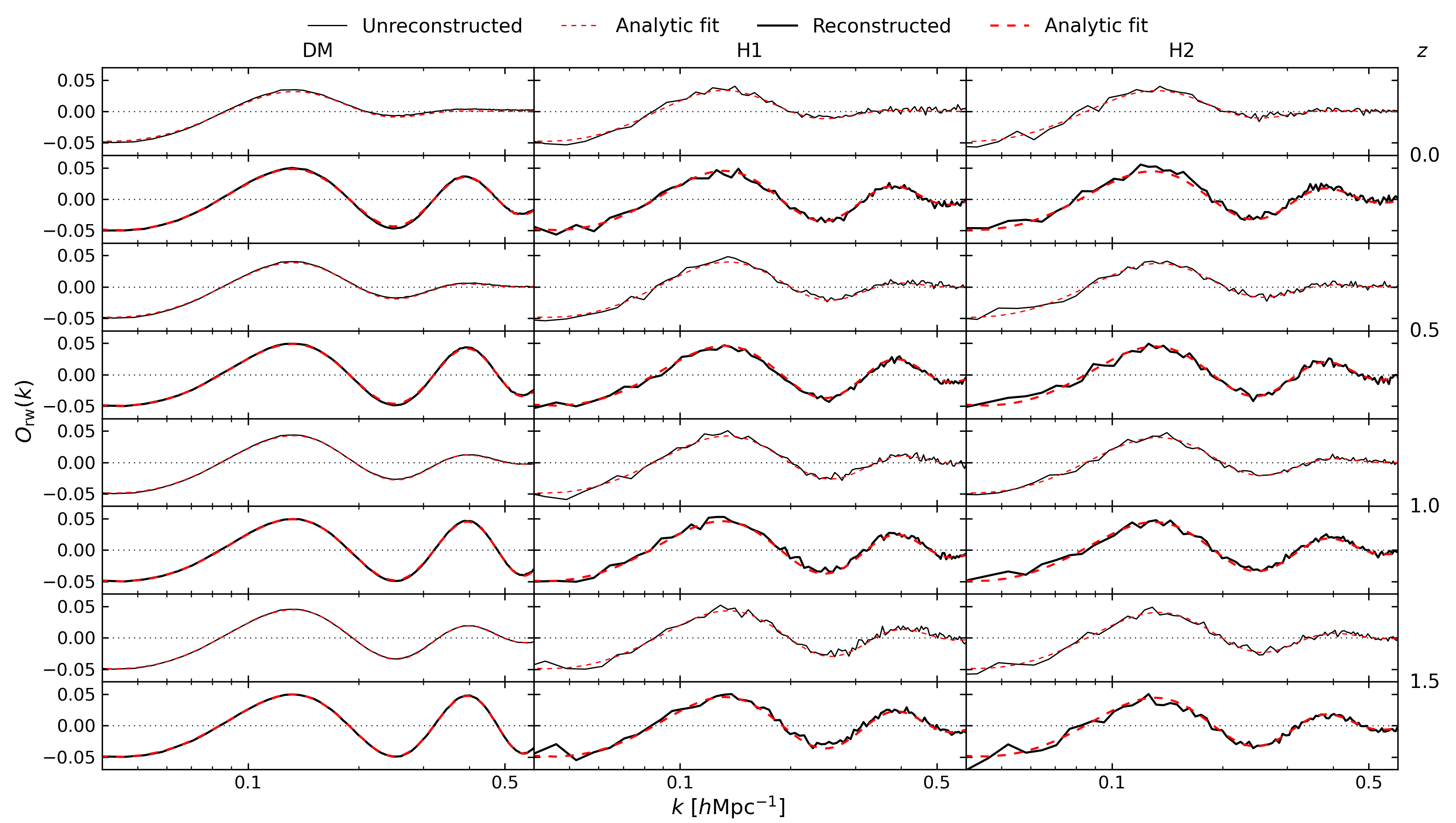
Figure 8: [Colour Online] The same as Fig. 5 but for Model 4.

References

- Achucarro et al. (2011) Achucarro A., Gong J.-O., Hardeman S., Palma G. A., Patil S. P., 2011, JCAP, 01, 030
- Adams et al. (2001) Adams J. A., Cresswell B., Easther R., 2001, Phys. Rev. D, 64, 123514
- Ade et al. (2014a) Ade P. A. R., et al., 2014a, Astron. Astrophys., 571, A22
- Ade et al. (2014b) Ade P. A. R., et al., 2014b, Astron. Astrophys., 571, A24
- Ade et al. (2016a) Ade P. A. R., et al., 2016a, Astron. Astrophys., 594, A17
- Ade et al. (2016b) Ade P. A. R., et al., 2016b, Astron. Astrophys., 594, A20
- Adshead et al. (2012) Adshead P., Dvorkin C., Hu W., Lim E. A., 2012, Phys. Rev. D, 85, 023531
- Aghanim et al. (2020) Aghanim N., et al., 2020, Astron. Astrophys., 641, A6
- Akrami et al. (2020a) Akrami Y., et al., 2020a, Astron. Astrophys., 641, A9
- Akrami et al. (2020b) Akrami Y., et al., 2020b, Astron. Astrophys., 641, A10
- Albrecht & Steinhardt (1982) Albrecht A., Steinhardt P. J., 1982, Phys. Rev. Lett., 48, 1220
- Alonso (2012) Alonso D., 2012, arXiv e-prints, p. arXiv:1210.1833
- Ballardini et al. (2016) Ballardini M., Finelli F., Fedeli C., Moscardini L., 2016, JCAP, 10, 041
- Ballardini et al. (2018) Ballardini M., Finelli F., Maartens R., Moscardini L., 2018, JCAP, 04, 044
- Ballardini et al. (2020) Ballardini M., Murgia R., Baldi M., Finelli F., Viel M., 2020, JCAP, 04, 030
- Bartolo et al. (2004) Bartolo N., Komatsu E., Matarrese S., Riotto A., 2004, Phys. Rept., 402, 103
- Bean et al. (2008) Bean R., Chen X., Hailu G., Tye S. H. H., Xu J., 2008, JCAP, 03, 026
- Behroozi et al. (2013) Behroozi P. S., Wechsler R. H., Wu H.-Y., 2013, Astrophys. J., 762, 109
- Beutler et al. (2019) Beutler F., Biagetti M., Green D., Slosar A., Wallisch B., 2019, Phys. Rev. Res., 1, 033209
- Birkin et al. (2019) Birkin J., Li B., Cautun M., Shi Y., 2019, Mon. Not. Roy. Astron. Soc., 483, 5267
- Cautun & van de Weygaert (2011) Cautun M. C., van de Weygaert R., 2011, arXiv e-prints, p. arXiv:1105.0370
- Chen (2010) Chen X., 2010, Adv. Astron., 2010, 638979
- Chen (2012) Chen X., 2012, JCAP, 01, 038
- Chen & Namjoo (2014) Chen X., Namjoo M. H., 2014, Phys. Lett. B, 739, 285
- Chen et al. (2007) Chen X., Easther R., Lim E. A., 2007, JCAP, 06, 023
- Chen et al. (2015) Chen X., Namjoo M. H., Wang Y., 2015, JCAP, 02, 027
- Chen et al. (2016) Chen X., Dvorkin C., Huang Z., Namjoo M. H., Verde L., 2016, JCAP, 11, 014
- Chen et al. (2020) Chen S.-F., Vlah Z., White M., 2020, JCAP, 11, 035
- Chluba et al. (2015) Chluba J., Hamann J., Patil S. P., 2015, Int. J. Mod. Phys. D, 24, 1530023
- Colombi & Novikov (2011) Colombi S., Novikov D., 2011, POWMES: Measuring the Power Spectrum in an N-body Simulation (ascl:1110.017)
- Crocce et al. (2006) Crocce M., Pueblas S., Scoccimarro R., 2006, Mon. Not. Roy. Astron. Soc., 373, 369
- DESI Collaboration et al. (2016) DESI Collaboration et al., 2016, arXiv e-prints, p. arXiv:1611.00036
- Debono et al. (2020) Debono I., Hazra D. K., Shafieloo A., Smoot G. F., Starobinsky A. A., 2020, Mon. Not. Roy. Astron. Soc., 496, 3448
- Doré et al. (2014) Doré O., et al., 2014, arXiv e-prints, p. arXiv:1412.4872
- Eisenstein et al. (2007) Eisenstein D. J., Seo H.-j., Sirko E., Spergel D., 2007, Astrophys. J., 664, 675
- Feldman et al. (1994) Feldman H. A., Kaiser N., Peacock J. A., 1994, Astrophys. J., 426, 23
- Flauger & Pajer (2011) Flauger R., Pajer E., 2011, JCAP, 01, 017
- Flauger et al. (2010) Flauger R., McAllister L., Pajer E., Westphal A., Xu G., 2010, JCAP, 06, 009
- Gao et al. (2012) Gao X., Langlois D., Mizuno S., 2012, JCAP, 10, 040
- Guth (1981) Guth A. H., 1981, Phys. Rev. D, 23, 347
- Hazra et al. (2010) Hazra D. K., Aich M., Jain R. K., Sriramkumar L., Souradeep T., 2010, JCAP, 10, 008
- Hazra et al. (2014) Hazra D. K., Shafieloo A., Smoot G. F., Starobinsky A. A., 2014, JCAP, 08, 048
- Hinshaw et al. (2013) Hinshaw G., et al., 2013, Astrophys. J. Suppl., 208, 19
- Huang et al. (2012) Huang Z., Verde L., Vernizzi F., 2012, JCAP, 04, 005
- Ivezić et al. (2019) Ivezić v., et al., 2019, Astrophys. J., 873, 111
- Kazin et al. (2014) Kazin E. A., et al., 2014, Mon. Not. Roy. Astron. Soc., 441, 3524
- Kobayashi et al. (2020) Kobayashi Y., Nishimichi T., Takada M., Takahashi R., Osato K., 2020, Phys. Rev. D, 102, 063504
- Komatsu et al. (2009) Komatsu E., et al., 2009, Astrophys. J. Suppl., 180, 330
- L’Huillier et al. (2018) L’Huillier B., Shafieloo A., Hazra D. K., Smoot G. F., Starobinsky A. A., 2018, Mon. Not. Roy. Astron. Soc., 477, 2503
- Lewis & Challinor (2011) Lewis A., Challinor A., 2011, CAMB: Code for Anisotropies in the Microwave Background (ascl:1102.026)
- Li et al. (2012) Li B., Zhao G.-B., Teyssier R., Koyama K., 2012, JCAP, 01, 051
- Li et al. (2013) Li B., Barreira A., Baugh C. M., Hellwing W. A., Koyama K., Pascoli S., Zhao G.-B., 2013, JCAP, 11, 012
- Linde (1982) Linde A. D., 1982, Phys. Lett. B, 108, 389
- Liu et al. (2020) Liu Y., Yu Y., Li B., 2020, arXiv e-prints, p. arXiv:2012.11251
- Mao et al. (2021) Mao T.-X., Wang J., Li B., Cai Y.-C., Falck B., Neyrinck M., Szalay A., 2021, Mon. Not. Roy. Astron. Soc., 501, 1499
- Palma et al. (2018) Palma G. A., Sapone D., Sypsas S., 2018, JCAP, 06, 004
- Peiris et al. (2003) Peiris H. V., et al., 2003, Astrophys. J. Suppl., 148, 213
- Racca et al. (2016) Racca G. D., et al., 2016, Proc. SPIE Int. Soc. Opt. Eng., 9904, 0O
- Sarpa et al. (2019) Sarpa E., Schimd C., Branchini E., Matarrese S., 2019, Mon. Not. Roy. Astron. Soc., 484, 3818
- Schaye et al. (2015) Schaye J., et al., 2015, Mon. Not. Roy. Astron. Soc., 446, 521
- Schmittfull et al. (2015) Schmittfull M., Feng Y., Beutler F., Sherwin B., Chu M. Y., 2015, Phys. Rev. D, 92, 123522
- Seo & Eisenstein (2003) Seo H.-J., Eisenstein D. J., 2003, Astrophys. J., 598, 720
- Shi et al. (2018) Shi Y., Cautun M., Li B., 2018, Phys. Rev. D, 97, 023505
- Slosar et al. (2019) Slosar A., Chen X., Dvorkin C., Meerburg D., Wallisch B., Green D., Silverstein E., 2019, BAAS, 51, 98
- Spergel et al. (2007) Spergel D. N., et al., 2007, Astrophys. J. Suppl., 170, 377
- Springel et al. (2018) Springel V., et al., 2018, Mon. Not. Roy. Astron. Soc., 475, 676
- Starobinsky (1992) Starobinsky A. A., 1992, Soviet Journal of Experimental and Theoretical Physics Letters, 55, 489
- Taylor & Kitching (2010) Taylor A. N., Kitching T. D., 2010, Mon. Not. Roy. Astron. Soc., 408, 865
- Tegmark (1997) Tegmark M., 1997, Phys. Rev. Lett., 79, 3806
- Teyssier (2002) Teyssier R., 2002, Astron. Astrophys., 385, 337
- Tinker et al. (2008) Tinker J. L., Kravtsov A. V., Klypin A., Abazajian K., Warren M. S., Yepes G., Gottlober S., Holz D. E., 2008, Astrophys. J., 688, 709
- Vasudevan et al. (2019) Vasudevan A., Ivanov M. M., Sibiryakov S., Lesgourgues J., 2019, JCAP, 09, 037
- Vlah et al. (2016) Vlah Z., Seljak U., Chu M. Y., Feng Y., 2016, JCAP, 03, 057
- Wang et al. (2017) Wang X., Yu H.-R., Zhu H.-M., Yu Y., Pan Q., Pen U.-L., 2017, Astrophys. J. Lett., 841, L29
- Wang et al. (2020) Wang Y., Li B., Cautun M., 2020, Mon. Not. Roy. Astron. Soc., 497, 3451
- Zeng et al. (2019) Zeng C., Kovetz E. D., Chen X., Gong Y., Muñoz J. B., Kamionkowski M., 2019, Phys. Rev. D, 99, 043517
- Zhai et al. (2019) Zhai Z., et al., 2019, Astrophys. J., 874, 95
- Zhu et al. (2017) Zhu H.-M., Yu Y., Pen U.-L., Chen X., Yu H.-R., 2017, Phys. Rev. D, 96, 123502