A Visibility Roadmap Sampling Approach for a Multi-Robot Visibility-Based Pursuit-Evasion Problem

Abstract

Given a two-dimensional polygonal space, the multi-robot visibility-based pursuit-evasion problem tasks several pursuer robots with the goal of establishing visibility with an arbitrarily fast evader. The best known complete algorithm for this problem takes time doubly exponential in the number of robots. However, sampling-based techniques have shown promise in generating feasible solutions in these scenarios. One of the primary drawbacks to employing existing sampling-based methods is that existing algorithms have long execution times and high failure rates for complex environments. This paper addresses that limitation by proposing a new algorithm that takes an environment as its input and returns a joint motion strategy which ensures that the evader is captured by one of the pursuers. Starting with a single pursuer, we sequentially construct Sample-Generated Pursuit-Evasion Graphs to create such a joint motion strategy. This sequential graph structure ensures that our algorithm will always terminate with a solution, regardless of the complexity of the environment. We describe an implementation of this algorithm and present quantitative results that show significant improvement in comparison to the existing algorithm.

I Introduction

Autonomous reconnaissance tasks, in which robots strive to observe salient features of objects or agents within their environments, remain one of the most active threads of research within the robotics community. Such tasks have wide-ranging application domains such as environmental monitoring [5, 6, 15, 39, 40], surveillance [1, 2, 4, 7], and search-and-rescue [13, 33, 24]. Many of these tasks can be framed as two-player games played amongst opposing teams: evaders (who wish to evade capture) and pursuers (who seek to capture them). This paper is concerned with a specific form of this two-player game, wherein a team of pursuers must locate an evader (or group of evaders) in a polygonal environment.

Specifically, we address one such problem where a group of pursuers, each equipped with an omni-directional sensor that extends to the polygonal boundary, must form a motion plan to locate an arbitrarily fast evader in a polygonal environment. Figure 1 illustrates this scenario. The literature has a number of results for this problem in the single-pursuer case, including algorithms with strong guarantees such as completeness [11] and path length optimality [37]. However, the case in which multiple pursuers cooperate is not nearly as well understood. A complete algorithm is known, but it runs in time doubly-exponential in the number of pursuers [34].

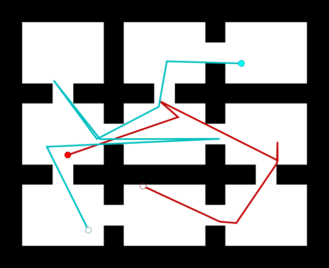
Figure 1: An example multi-pursuer solution strategy generated by the proposed algorithm. The filled circle represent the initial location of the pursuer, while the hollow circles represent its final location.

One approach to overcome the computational challenge posed by this multiple-pursuer pursuit-evasion planning task [35], showed the feasibility of sampling-based techniques to generate joint motion strategies. Nevertheless, that approach has several important limitations.

1. The existing algorithm lacks insight into how the sampling should be performed, and treats the sampling distribution as a “black box.”

2. The existing algorithm requires a predetermined number of pursuers as input; it cannot adapt the number of pursuers to the complexity of the environment.

3. The solutions generated by this approach are of poor quality, in the sense that there nearly always are motions by one or more of the pursuers that do not actively contribute to the search.

After a review of related work (Section II), precise statement of the problem (Section III), and a summary of important concepts from prior work on this problem (Section IV), this paper makes three new contributions that address the limitations of the existing algorithm.

1. We introduce a new sampling strategy, tailored to the visibility-based nature of the problem (Section V-A).

2. We describe a method that eliminates the need for the number of pursuers to be provided as input, instead iteratively increasing the size of the team (Section V-B).

3. We present a post-processing algorithm that improves solution quality (Section V-C).

Finally, Section VI presents quantitative evaluations of these new improvements and Section VII previews future work.

II Related work

This research blends ideas from two vibrant threads of prior robotics research: visibility-based pursuit-evasion and sampling-based motion planning in high dimensional spaces.

In regard to pursuit-evasion, this work is most closely aligned with the problem first introduced by Suzuki and Yamashita [38], in which an evader operating in a geometric environment seeks to locate an unpredictable evader capable of moving arbitrarily quickly. This work was later expanded by Guibas, Latombe, LaValle, Lin, and Motwani [11] who provide a complete algorithm for the single pursuer scenario in simply-connected environments for a pursuer with an omnidirectional field-of-view. Park, Lee, and Chwa [25] identified necessary and sufficient conditions for a search to be feasible for a single pursuer.

Other results for the single pursuer scenario that build upon this foundation provide results such as completeness [11], optimality [37], establishing and maintaining visibility of a moving agent [29, 30] or consider more restrictive scenarios with respect to pursuer parameters such as sensing, actuation and speed [27, 9, 41, 26, 36, 28].

The community has placed increased emphasis on the study of richer scenarios where a team of pursuers cooperate during the search [20, 16, 10, 35, 14, 19, 8]. Stiffler and O’Kane [34] present an algorithm utilizing a cylindrical algebraic decomposition that, while complete, relies upon constructing a graph whose size is doubly exponential in the complexity of the environment. That work subsequently served as motivation for approaches that utilize heuristics [35] that seek to overcome the problem complexity by utilizing sampling techniques.

More generally, sampling based techniques have been employed in a number of planning contexts where computing an exact solution proves computationally intractable such as motion planning [18, 23, 22, 32, 17] and manipulation planning [31, 12, 21]. One caveat of sampling-based methods is that they quite often suffer from the curse of dimensionality [3] whereby, as the number of dimensions increases, the search space becomes so vast that the number of samples required for adequate coverage of the space increases dramatically. A number of different approaches have been proposed to combat this problem. One recent result draws samples in lower-dimensional subspaces to search for a feasible solution, and incrementally reasons about higher dimensions while utilizing the information gained in the lower dimensional graph [43]. For the specific multi-robot case in which the configuration space is a Cartesian product of the configuration spaces of individual agents in the system, one novel approach seeks to reason about each agent independently (a subdimension), and only when the agents reach a point where they interact with one another is there a lifting to a higher-dimensional space [42].

III Problem statement

III-A The environment, the evader, and the pursuers

Let $E\subset\mathbb{R}^{2}$ be a bounded, closed, connected polygonal set called the environment. An evader moves within $E$. We describe the evader’s position via a continuous function $e(t):[0,\infty)\rightarrow E$ to represent the location of the evader at time $t$. There is no restriction on the speed of the evader, so long as it is finite.

We task $n$ pursuers with the goal of ensuring capture of the evaders regardless of the evader trajectories. We can assume worst case reasoning in the sense that there is a singular evader which follows a path that maximizes its time until detection over all evader trajectories. We consider both scenarios in which the number of pursuers is known and fixed, an in which the number of pursuers to utilize is determined by the algorithm as the plan is generated. Let $p_{i}:[0,\infty)\rightarrow E$ represent the location of the $i^{\text{th}}$ pursuer as a function of time. We refer to such functions as motion strategies. Each pursuer is equipped with knowledge of $E$ and an omnidirectional sensor which extends until the nearest point on the boundary of $E$ in each direction. That is, a pursuer at point $q_{1}\in E$ can see every point in its visibility polygon, $V(q_{1})=\{q_{2}\in E\mid\overline{q_{1}q_{2}}\subseteq E\}$ where $\overline{q_{1}q_{2}}$ denotes the line segment joining $q_{1}$ and $q_{2}$ in $E$.

Figure 2: Example evader and pursuer paths. The evader is detected at time $t$.

III-B Objective

The algorithmic problem we address is to find a collection of motion strategies $\{p_{1},p_{2},\dots,p_{n}\}$ such that, for some $t\geq 0$ and $j\in\{1,\dots,n\}$, $e(t)\in V(p_{j}(t))$ for any evader curve $e$. Such a collection of motion strategies is called a solution. Specifically, we consider two related problems.

Fixed

Given an environment $E$ and a positive integer $n$, generate a solution using exactly $n$ pursuers. Algorithms for this problem can be evaluated by examining both the time needed to generate a solution as well as the time needed for the pursuers to execute that solution.

Variable

Given an environment $E$, generate a solution that uses as few pursuers as possible. In addition to the run time and execution time criteria mentioned above, algorithms for this variant of the problem can also be judged by the number of pursuers utilized by the computed solution.

IV Background

This section concisely summarizes some essential prior results upon which our new contributions build. Specifically, we describe how the pursuers’ knowledge about the evader’s possible position can be maintained (Section IV-A) and present a data structure that encapsulates the progress of a search for a complete solution (Section IV-B).

IV-A Shadows and shadow events

In general, the pursuers will be able to see only a subset of the environment at any particular time, while the remaining parts of the environment are out of view of all of the pursuers. Formally, at time $t$, the shadow region, $S(t)$, is $E\setminus\bigcup_{i=1}^{n}V(p_{i}(t))$. We call the maximally path-connected components of $S(t)$ shadows.

Figure 3: An example of a cleared (right) and contaminated (left) shadow, given the pursuer’s movement history. Here, the white region displays the visibility polygon of a pursuer located at the red circle.

The crucial information about each shadow is whether or not the evader may be hiding within that shadow. A shadow $s$ is called cleared at time $t$ if, based on the pursuers’ joint motions up to time $t$, it is not possible for the evader to be within $s$ without having been seen by one of the pursuers. Analogously, a shadow is said to be contaminated if it is possible for the evader to be hiding within it given the pursuers’ motions up to time $t$. As the pursuers move through the environment, the individual shadows change continuously. However, the cardinality of the set of shadows changes only when a shadow event occurs, i.e. a shadow appears, disappears, splits, or merges with another shadow. The shadow events induce the following changes to the status of a shadow:

• Appear: A shadow can appear if the pursuers lose vision of a region within the environment. In this event, the new shadow has a cleared status.

• Disappear: A shadow can disappear if the pursuers gain vision of a region which was previously a shadow. The label corresponding to the shadow that disappears is discarded.

• Merge: Two or more shadows can merge into a larger shadow. In this event, the new shadow is assigned the label cleared only if all merging shadows were cleared; otherwise, the new shadow is labeled contaminated.

• Split: If a shadow becomes path disconnected, we say it was split. The newly formed shadows have the status of the initial from which they were formed.

More detail about these types of shadow events and their clear/contaminated labels may be found in the work of Guibas, Latombe, LaValle, Lin, and Motwani [11].

IV-B Sample-generated pursuit-evasion graphs

To aid in the search for a joint motion strategy for the pursuers, we utilize the Sample-Generated Pursuit-Evasion Graph (SG-PEG) data structure; additional details about the SG-PEG appear in the original paper [35]. An SG-PEG is a directed graph $G=(V_{G},E_{G})$, representing a portion of the connectivity of the joint configuration space for a fixed number $n$ of pursuers. Each vertex in $V_{G}$ represents a joint configuration for the pursuers $(p_{1},\dots,p_{n})\in E^{n}$. Edges in $E_{G}$ connect pairs of vertices for which it is possible for each pursuer to make a collision-free straight line motion between the two corresponding configurations. That is, if an edge exists between two vertices representing joint configurations $(p_{1},\dots,p_{n})$ and $(q_{1},\dots,q_{n})$, then $\overline{p_{i}q_{i}}\subset E$ for each $i\in\{1,\ldots,n\}$. One vertex, corresponding to the starting joint configuration of the robots, is designated as the root of the graph. Each vertex maintains a list of non-dominated shadow labels (i.e. clear/contaminated statuses) that are reachable by traversing the graph along some (possibly non-simple) path from the root.

The primary operation that can be performed on a standard SG-PEG is AddSample$(p_{1},\dots,p_{n})$ which, given a collision-free joint configuration, performs three main steps:

• It inserts a new vertex $v$ at the given joint configuration.

• For any other vertex $u$ within a pre-defined connection distance in $E^{n}$, it checks whether the straight-line connection between $v$ and $u$ would be collision-free. If so, and if the shortest path in the graph between $v$ and $u$ is sufficiently long, it creates edges $vu$ and $uv$.

• For each new edge thusly added, AddSample computes the shadow events described in Section IV-A induced by motion along that edge. It then propagates the reachable shadow label information across the new edge and then recursively across the graph, to determine what new reachable shadow labels, if any, are now possible at which vertices, due to this new edge.

The utility of the SG-PEG is that if any vertex $v$ has a reachable shadow label that is fully cleared (i.e. it has a reachable shadow label set in which each shadow bears a clear label), then a solution can be extracted from the graph by tracing back via the appropriate edges to the root vertex.

V Algorithm description

Our approach to this problem is based on two significant additions and one modification to the prior algorithm of Stiffler and O’Kane [35]. The basic idea of that prior algorithm is to generate random samples in $E^{n}$ and use them to construct an SG-PEG, continuing until the SG-PEG indicates that it contains a solution. Algorithm 1 shows the enhancements that we propose. New elements in comparison to the prior algorithm are highlighted: modifications to the sampling strategy in purple text and new additions in blue text. Note that, $n$, the number of robots has been removed in our variant. Details about these changes appear below.

Algorithm 1 Solve($E$, $n$, $C$, $S$)

1:an environment $E$, a number of pursuers $n$,
     an expansion criterion $C$ and a sampler $S$

2:$G\leftarrow$ empty SG-PEG for $n$ pursuers 1 pursuer

3:$p\leftarrow{\color[rgb]{.75,0,.25}\textsc{S.getSample}()}$

4:$G.\textsc{addSample}(p)$

5:$G.\textsc{setRoot}(p)$

6:while no solution has been found do

7:    $p\leftarrow{\color[rgb]{.75,0,.25}S.\textsc{getSample}()}$

8:    $G.\textsc{addSample}(p)$

9:    if $C$ is met then

10:         ${\color[rgb]{0,0,1}G.\textsc{addPursuer}()}$     

11:$X\leftarrow\textsc{extractSolution}()$

12:${\color[rgb]{0,0,1}X^{\prime}\leftarrow\textsc{refineSolution}(X)}$

13:return $X^{\prime}$

V-A Web sampling

Stiffler and O’Kane proposed a handful of sampling distributions, but none of them proved significantly more effective than simple uniform random sampling of the joint configuration space. This approach appears not to be particularly effective in this domain, because the environment is comprised of regions whose surveyance is essential to finding a solution. To combat this issue, we propose a new strategy for generating samples, which specifically takes into account the visibility component of the problem. Specifically, the goal is to generate a small collection of samples $W$ that has two properties: (a) each point in $E$ is seen by at least one point in $W$, and (b) a pursuer moving between points in $W$ along straight line segments in $E$ can travel between any pair of points in $W$, i.e. $W$ forms a ‘connected roadmap’ of $E$.

The approach is based on a randomized structure called a web in $E$, which is constructed in two steps. First, we construct a set of initial points $P\subset E$. Each initial point is selected sequentially and randomly, from the region outside the union of visibility polygons of the previously selected points. The process continues until $\bigcup_{p\in P}V(p)=E$. Then the algorithm selects a collection of intersection points $Q\subseteq E$ by examining pairs of initial points $\{p_{i},p_{j}\}\subseteq P$, and placing a point uniformly at random within $V(p_{i})\cap V(p_{j})$, if that intersection is non-empty. A web is simply the combination $W=P\cup Q$. Figure 4 illustrates this concept.

We utilized webs to generate samples from $E^{n}$ in Lines 3 and 7 by generating a separate web for each pursuer and sampling, without replacement, from those points. If the points in any of the webs are exhausted, we generate another set of webs and continue.

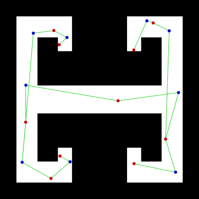
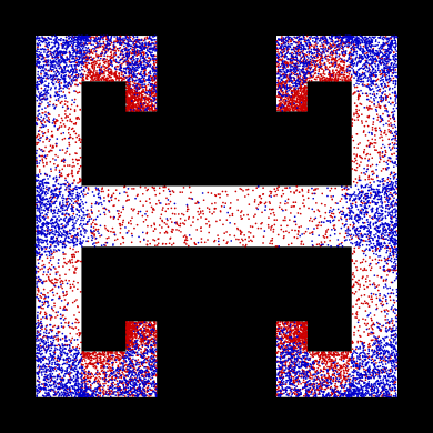
Figure 4: [left] An example web. Red points are initial points; the blue are intersection points. Green edges connect each intersection point to the initial points from which it is induced. [right] The distribution induced by web sampling, based upon 750 generated webs. Note the higher density at junctions and corners.

V-B Variable numbers of pursuers

In the prior algorithm, the number of pursuers in the solution was required as an input. This information was necessary because the SG-PEG data structure stores joint configurations drawn from $E^{n}$; thus $n$ must be known to construct an SG-PEG.

To alleviate this limitation, we instead propose a sequential process, in which the number of pursuers is gradually increased as the algorithm proceeds. Realizing this approach in the planner requires us to resolve two complications.

First, the algorithm requires a mechanism to transition, in mid-stream, from an $n$-pursuer SG-PEG to an $(n+1)$-pursuer SG-PEG (Line 10). One straightforward approach is to simply discard the existing vertices and edges and restart the search with an additional pursuer. (This is referred to as the ‘Clear’ option in Section VI.)

However, it may be preferable to ensure that our previous effort is not wasted. To this end, we propose a new method that clones the first pursuer in each vertex of the SG-PEG. That is, for each vertex in the SG-PEG, we replace its joint configuration $(p_{1},p_{2},\dots,p_{n})$ with $(p_{1},p_{2},\dots,p_{n},p_{1})$. This adds an additional pursuer to the graph, without changing any of the reachable labels or edges. Thus, the cloning option is extremely efficient, but it leads to an SG-PEG in which the newly-added pursuer moves in parallel with another pursuer. Future edges added at the $(n+1)$-th layer will correspond to independent motions for these two robots (as they draw from their own unique set of webs).

Next, we must decide when to expand the number of pursuers (Line 9). We consider two options. First, we propose a method that devotes fixed effort to each stage of the search. The process begins by rapidly generating a trivial solution by placing pursuers until their visibility fully covers the environment, which results in a solution that requires no movement from the pursuers. This gives a (generally very loose) upper bound $N$ on the number of pursuers required. Then, given a target total run time of $T_{\text{limit}}$ seconds, we apportion the time between the possible numbers of pursuers $1,\ldots,N$ via a Poisson distribution. The Poisson distribution was selected due to the placement of the mean, as well as its skew and shape. We choose a tunable parameter $\alpha$ which determines the fraction of time to spend on the final step that utilizes $N$ pursuers, so that according to the definition of the Poisson distribution, we have $\alpha=\lambda^{N}e^{-\lambda}/N!$. From this equation, the algorithm numerically computes the Poisson parameter $\lambda$ and allocates $T_{\text{limit}}\lambda^{i-1}e^{-\lambda}/(i-1)!$ to the search with $i$ pursuers before proceeding to $i+1$. Because of the existence of the upper bound $N$, this method will always produce a solution, although it may require a large number of pursuers.

As an alternative, we also consider a stalled progress approach, based upon monitoring the minimum sum of the contaminated shadow area across all vertices of the graph. (n.b. We have a solution if and only if this value reaches $0$.) If this value fails to improve by at least 5% after adding $M$ samples, we add a new pursuer. To enable a fair comparison to the fixed effort method, we once again return a trivial solution if no solution is found with fewer pursuers.

V-C Solution refinement

Because of the sampling-based nature of this algorithm, its outputs are likely to have extraneous motions. This issue is noticeably more severe in our context than for traditional sampling-based motion planning because the generated solutions may travel several times along certain edges in an effort to clear specific shadows. In this section, we introduce a post processing method which takes a joint motion strategy and optimizes it by removing unnecessary pursuer motions.

Our method is similar to standard shortcut-based path smoothing. We select two points $z_{a}$ and $z_{b}$ at distance $c$ along the solution path in $E^{n}$, and check whether taking a shortcut directly from $z_{a}$ to $z_{b}$ yields a path that is still a correct solution. Figure 5 depicts the process. Our check features one important difference from traditional path smoothing: In addition to ensuring that the refined solution is collision-free, we must also ensure that it remains a correct solution, i.e. that the refinement does not allow any shadows to remain contaminated. We do this by tracking forward through the shortened path, applying the shadow events experienced along that path —Recall Section IV-A— to update the shadow labels.

Given this shortcut operation, we greedily optimize the path, proceeding systematically over decreasing values of $c$ and increasing positions of $z_{a}$. (From these two, $z_{b}$ is readily computed.) Each time we discover a shortcut yielding a correct solution, that shortened solution replaces the previous solution, and the process continues. See Figure 6.

Figure 5: A cut of length $c$ during solution refinement.

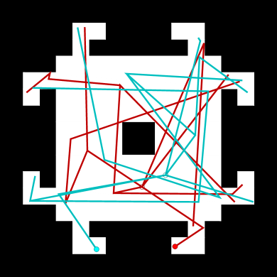
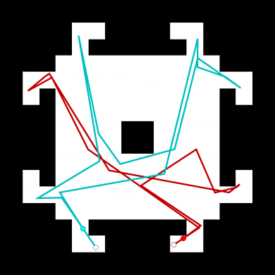
Figure 6: Refining a solution. [left] Before. [right] After.

VI Evaluation

Table I: Simulation results for the Office environment (Figure 1).

	success	comp time (s)		num robots		num vertices		num edges
	rate	$\mu$	$\sigma$	$\mu$	$\sigma$	$\mu$	$\sigma$	$\mu$	$\sigma$
WS   ($n=2$)	100%	87.201	58.707	2.000	0.000	74.360	50.392	137.440	103.644
SO14 ($n=2$)	96%	96.890	78.231	2.000	0.000	117.875	62.007	219.167	131.542
WS   ($n=3$)	100%	68.953	56.738	3.000	0.000	109.160	55.984	157.040	105.265
SO14 ($n=3$)	100%	63.205	25.110	3.000	0.000	330.440	210.853	542.080	453.409
WS   ($n=4$)	100%	57.248	52.329	4.000	0.000	177.760	73.723	167.960	103.567
SO14 ($n=4$)	100%	73.448	65.325	4.000	0.000	1258.480	774.096	1830.920	1655.530
WS   ($n=5$)	100%	91.633	80.529	5.000	0.000	392.520	229.407	275.920	224.627
SO14 ($n=5$)	80%	235.866	129.786	5.000	0.000	4081.000	1361.404	4495.150	2546.067
FE Clone $(\alpha=0.001)$	100%	138.097	71.992	3.440	0.768	138.720	88.246	186.720	89.464
FE Clear $(\alpha=0.001)$	100%	111.114	112.003	3.280	2.390	866.360	2702.653	732.200	1379.524
SP Clone $(M=30)$	100%	193.867	55.951	2.520	2.365	117.280	79.072	192.200	120.596
SP Clear $(M=30)$	100%	84.824	29.878	7.640	4.636	222.360	107.938	185.160	35.873

Table II: Simulation results for the H environment (Figure 4).

	success	comp time (s)		num robots		num vertices		num edges
	rate	$\mu$	$\sigma$	$\mu$	$\sigma$	$\mu$	$\sigma$	$\mu$	$\sigma$
WS   ($n=2$)	100%	18.716	9.816	2.000	0.000	71.600	49.019	119.160	103.625
SO14 ($n=2$)	100%	33.885	14.777	2.000	0.000	105.760	77.638	193.640	158.844
WS   ($n=3$)	100%	20.151	11.281	3.000	0.000	143.200	46.871	168.720	84.149
SO14 ($n=3$)	100%	35.965	20.354	3.000	0.000	212.560	152.480	349.840	305.536
WS   ($n=4$)	100%	27.131	10.502	4.000	0.000	261.520	94.841	211.920	116.173
SO14 ($n=4$)	96%	43.636	42.848	4.000	0.000	639.042	365.724	972.042	704.745
WS   ($n=5$)	100%	47.967	24.342	5.000	0.000	413.840	119.927	196.800	77.066
SO14 ($n=5$)	96%	81.949	62.208	5.000	0.000	1743.708	1512.375	2422.125	2732.005
FE Clone $(\alpha=0.001)$	100%	27.065	9.973	2.000	0.000	48.120	16.269	79.440	31.466
FE Clear $(\alpha=0.001)$	100%	21.538	8.483	2.000	0.000	71.360	24.124	115.520	48.321
SP Clone $(M=30)$	100%	42.422	13.620	2.400	1.607	76.120	29.992	129.320	46.703
SP Clear $(M=30)$	100%	19.637	6.906	7.920	3.081	204.840	62.487	136.640	31.579

Table III: Simulation results for the Spider environment (Figure 6).

	success	comp time (s)		num robots		num vertices		num edges
	rate	$\mu$	$\sigma$	$\mu$	$\sigma$	$\mu$	$\sigma$	$\mu$	$\sigma$
WS   ($n=2$)	100%	151.738	87.515	2.000	0.000	54.240	34.170	90.920	65.193
SO14 ($n=2$)	84%	312.341	115.955	2.000	0.000	152.952	90.760	296.619	182.206
WS   ($n=3$)	100%	91.825	41.326	3.000	0.000	50.120	36.003	68.280	58.533
SO14 ($n=3$)	96%	211.234	89.930	3.000	0.000	90.167	33.983	160.750	65.811
WS   ($n=4$)	100%	84.356	26.550	4.000	0.000	55.520	26.590	61.880	40.169
SO14 ($n=4$)	96%	216.941	83.815	4.000	0.000	142.708	283.093	257.083	560.368
WS   ($n=5$)	100%	92.822	42.587	5.000	0.000	75.800	33.582	72.920	47.970
SO14 ($n=5$)	92%	222.129	77.185	5.000	0.000	81.261	31.517	123.087	55.083
FE Clone $(\alpha=0.001)$	100%	249.742	116.423	5.080	1.631	107.720	40.658	117.200	46.227
FE Clear $(\alpha=0.001)$	100%	258.762	124.280	5.080	2.159	196.200	188.685	184.200	110.659
SP Clone $(M=30)$	88%	403.098	91.530	3.727	0.827	163.682	35.301	275.955	50.614
SP Clear $(M=30)$	100%	236.300	134.572	4.200	4.021	139.680	102.347	184.440	65.614

This section evaluates the performance of the proposed approach. We implemented the algorithm in C++ and executed it on a computer with an Intel i7-7500U processor and 12GB of memory, running Ubuntu 18.04.2 64-bit.

We performed simulations in the environments shown in Figures 1 (Office), 4 (H), and 6 (Spider). This selection of environments is intended to provide a variety common environmental traits. The H environment contains narrow corridors, the Spider environment possesses numerous hard to reach areas, and the Office environment is somewhat uniformly spread out, with a complex boundary.

We generated solution strategies for these environments using both classes of algorithms described thus far: those that utilize a fixed number of pursuers and those that can vary the number of pursuers. In the former case, we considered both web sampling (WS) and uniform random sampling (SO14) [35] and varied the fixed number of robots between 2 and 5. In the latter case, we considered all four combinations of expansion criterion (fixed effort (FE) or stalled progress (SP)) and graph expansion method (clone pursuer (Clone) or clear progress (Clear)).

For each of these scenarios, we executed 25 trials and recorded the computation time in seconds, number of pursuers used in the returned solution, as well as the total numbers of vertices and edges generated. Each experiment was allotted 10 minutes of computation time; if no solution was produced in that time, we considered the trial to be a failure. Failed trials are excluded from the statistics, but it should be noted that if they were included, they would contribute a run time of at least 10 minutes. The results, summarized via the means $(\mu)$ and standard deviations $(\sigma)$, appear in Tables II, I and III. A number of conclusions may be drawn from the results.

WS improves performance over SO14

First, in all of the tested environments, our WS method outperformed SO14 by a wide margin. The smallest improvement in computation time occurred in the Office environment, perhaps due to the uniform nature of the environment and the complexity of the geometry calculations.

Clone and Clear appear to be complementary

For the simulations with a variable number of pursuers, we look to compare the performance between the cloning method and the clear method when expanding a graph. When using FE as the expansion criterion, the results are remarkably similar between the two methods. At first glance, one may assume the cloning method should outperform the clearing method due to the larger amount of information the graph contains. This however, is not always the case, because an increased number of vertices means an increased amount of time to add each new sample, due to the propagation of reachable labels across the graph. When SP was the expansion criterion, clearing has a faster computation time, but also a much higher mean and standard deviation for the number of pursuers. It was often the case that SP with clearing would return a trivial solution, as the algorithm cleared a substantial amount of meaningful calculations performed.

Allowing the number of pursuers to vary incurs only a modest computational cost

Lastly, we compare the fixed number of pursuers using WS, to the variable number of pursuers methods. For each environment, the run times of the variable number of pursuers were within approximately a factor of 2 of that of the fixed number of pursuers. A portion of this additional time comes from the variable number of pursuers constructing a single pursuer graph, in environments which all require at least 2 pursuers to solve.

Finally, for each environment, we refined all 25 solutions generated by WS with 2 pursuers. The results are summarized in Table IV, which shows the mean and standard deviation of the computation time (in seconds) along with the length of the solution path (in meters) before and after it was refined. The results show that this approach effectively and consistently reduces the path lengths.

Table IV: Refinement results for the solutions produced by WS ($n=2$).

	comp		length		length
	time (s)		before (m)		after (m)
	$\mu$	$\sigma$	$\mu$	$\sigma$	$\mu$	$\sigma$
Office	29.6	37.5	254.5	114.5	136.9	97.4
H	6.4	5.6	256.5	109.4	100.0	31.7
Spider	50.9	61.9	360.3	222.3	168.8	139.0

VII Conclusion

This paper presents a sampling-based algorithm for a visibility-based pursuit-evasion problem that generates a joint motion strategy for a team of robots in a polygonal environment. The three primary contributions are a novel sampling strategy for this domain, an iterative algorithm for generating a joint motion strategy for the pursuers, and a post-processing path-smoothing algorithm that refines the strategy returned by the main algorithm. The algorithm was shown to outperform existing techniques.

Future work might build upon the results in this paper. First, possibilities remain for enhancing the post processing step. There remain a number of open questions on how these kinds of path smoothing algorithms can be best applied to the pursuit-evasion domain. Second, is the development of an anytime algorithm that begins with an uninteresting solution —for example, one utilizing enough pursuers to ensure that their visibility polygons fully cover the environment— and attempts to work backwards, eliminating robots, by searching for solutions in the reduced joint sub-space.

[sorting=nyt]

References

- [1] Jose J. Acevedo, Begoña C. Arrue, Ivan Maza and Anibal Ollero “A Decentralized Algorithm for Area Surveillance Missions Using a Team of Aerial Robots with Different Sensing Capabilities” In Proc. IEEE International Conference on Robotics and Automation, 2014
- [2] Tauhidul Alam, Md Mahbubur Rahman, Leonardo Bobadilla and Brian Rapp “Multi-Vehicle Patrolling with Limited Visibility and Communication Constraints” In Military Communications Conference, 2017, pp. 465–479
- [3] R. Bellman “Dynamic Programming” Princeton, NJ: Princeton University Press, 1957
- [4] Philip Dames, Pratap Tokekar and Vijay Kumar “Detecting, localizing, and tracking an unknown number of moving targets using a team of mobile robots” In International Journal of Robotics Research 36.13-14, 2017, pp. 1540–1553
- [5] M. Duarte et al. “Application of swarm robotics systems to marine environmental monitoring” In MTS/IEEE OCEANS - Shanghai, 2016 DOI: 10.1109/OCEANSAP.2016.7485429
- [6] Matthew Dunbabin and Lino Marques “Robots for Environmental Monitoring: Significant Advancements and Applications” In IEEE Robotics and Automation Magazine 19, 2012, pp. 24–39
- [7] S.. Feng, S.. Han, K. Gao and J. Yu “Efficient Algorithms for Optimal Perimeter Guarding” In Proc. Robotics: Science and Systems, 2019
- [8] A. Ganguli, J. Cortes and F. Bullo “Visibility-based multi-agent deployment in orthogonal environments” In 2007 American Control Conference, 2007, pp. 3426–3431 DOI: 10.1109/ACC.2007.4283034
- [9] B.. Gerkey, S. Thrun and G. Gordon “Visibility-based Pursuit-evasion with Limited Field of View.” In International Journal of Robotics Research 25.4, 2006, pp. 299–315
- [10] Livia Gregorin et al. “Heuristics for the Multi-Robot Worst-Case Pursuit-Evasion Problem” In IEEE Access 5, 2017, pp. 17552–17566
- [11] L.. Guibas et al. “Visibility-Based Pursuit-Evasion in a Polygonal Environment” In International Journal on Computational Geometry and Applications 9.5, 1999, pp. 471–494
- [12] Kris Hauser “The Minimum Constraint Removal Problem with Three Robotics Applications” In International Journal of Robotics Research 33.1, 2014, pp. 5–17
- [13] G. Hollinger, A. Kehagias and S. Singh “Probabilistic Strategies for Pursuit in Cluttered Environments with Multiple Robots” In Proc. IEEE International Conference on Robotics and Automation, 2007
- [14] V. Isler, S. Kannan and S. Khanna “Randomized pursuit-evasion in a polygonal environment” In IEEE Transactions on Robotics 21.5, 2005, pp. 875–884 DOI: 10.1109/TRO.2005.851373
- [15] Volkan Isler et al. “Finding and tracking targets in the wild: Algorithms and field deployments” In Proc. IEEE International Symposium on Safety, Security, and Rescue Robotics, 2015
- [16] Francesco Bullo Joseph W. “Distributed pursuit-evasion without mapping or global localization via local frontiers” In Autonomous Robots 32, 2012, pp. 81–95
- [17] S. Karaman and E. Frazzoli “Sampling-based Algorithms for Optimal Motion Planning” In International Journal of Robotics Research 30.7, 2011, pp. 846–894
- [18] L.. Kavraki, P. Svestka, J.-C. Latombe and M.. Overmars “Probabilistic Roadmaps for Path Planning in High-Dimensional Configuration Spaces” In IEEE Transactions on Robotics and Automation 12.4, 1996, pp. 566–580
- [19] A. Kolling and S. Carpin “The GRAPH-CLEAR problem: definition, theoretical properties and its connections to multirobot aided surveillance” In 2007 IEEE/RSJ International Conference on Intelligent Robots and Systems, 2007, pp. 1003–1008 DOI: 10.1109/IROS.2007.4399368
- [20] A. Kolling and S. Carpin “Multi-robot pursuit-evasion without maps” In Proc. IEEE International Conference on Robotics and Automation, 2010, pp. 3045–3051
- [21] A. Krontiris and K.. Bekris “Efficiently Solving General Rearrangement Tasks: A Fast Extension Primitive for an Incremental Sampling-based Planner” In Proc. IEEE International Conference on Robotics and Automation, 2016
- [22] S.. LaValle and J.. Kuffner “Rapidly-Exploring Random Trees: Progress and Prospects” In Proc. Workshop on the Algorithmic Foundations of Robotics, 2000
- [23] J. Marble and K.. Bekris “Asymptotically Near-Optimal Planning with Probabilistic Roadmap Spanners” In IEEE Transactions on Robotics 29.2, 2013, pp. 432–444
- [24] N. Mimmo, P. Bernard and L. Marconi “Avalanche victim search via robust observers” In Proc. IEEE International Conference on Robotics and Automation, pp. 4066–4072 DOI: 10.1109/ICRA40945.2020.9196646
- [25] S. Park, J. Lee and K. Chwa “Visibility-Based Pursuit-Evasion in a Polygonal Region by a Searcher” In Proc. International Colloquium on Automata, Languages and Programming Springer-Verlag, 2001, pp. 281–290
- [26] S. Rajko and S.. LaValle “A Pursuit-Evasion Bug Algorithm” In Proc. IEEE International Conference on Robotics and Automation, 2001, pp. 1954–1960
- [27] S. Sachs, S.. LaValle and S. Rajko “Visibility-Based Pursuit-Evasion in an Unknown Planar Environment” In International Journal of Robotics Research 23.1, 2004, pp. 3–26 DOI: 10.1177/0278364904039610
- [28] Florian Shkurti and Gregory Dudek “On the complexity of searching for an evader with a faster pursuer” In Proc. IEEE International Conference on Robotics and Automation, 2013, pp. 4062–4067 DOI: 10.1109/ICRA.2013.6631150
- [29] Florian Shkurti and Gregory Dudek “Topologically distinct trajectory predictions for probabilistic pursuit” In Proc. IEEE/RSJ International Conference on Intelligent Robots and Systems, 2017, pp. 5653–5660 DOI: 10.1109/IROS.2017.8206454
- [30] Florian Shkurti, Nikhil Kakodkar and Gregory Dudek “Model-Based Probabilistic Pursuit via Inverse Reinforcement Learning” In Proc. IEEE International Conference on Robotics and Automation, 2018, pp. 7804–7811 DOI: 10.1109/ICRA.2018.8463196
- [31] T. Siméon, J.-P. Laumond, J. Cortés and A. Sahbani “Manipulation Planning with Probabilistic Roadmaps” In International Journal of Robotics Research, 2004
- [32] K. Solovey, O. Salzman and D. Halperin “Finding a Needle in an Exponential Haystack: Discrete RRT for Exploration of Implicit Roadmaps in Multi-Robot Motion Planning” In Proc. Workshop on the Algorithmic Foundations of Robotics, 2014
- [33] N.. Stiffler and J.. O’Kane “Visibility-Based Pursuit-Evasion with Probabilistic Evader Models” In Proc. IEEE International Conference on Robotics and Automation, 2011, pp. 4254–4259
- [34] N.. Stiffler and J.. O’Kane “A Complete Algorithm for Visibility-Based Pursuit-Evasion with Multiple Pursuers” In Proc. IEEE International Conference on Robotics and Automation, 2014, pp. 1660–1667
- [35] N.. Stiffler and J.. O’Kane “A Sampling Based Algorithm for Multi-Robot Visibility-Based Pursuit-Evasion” In Proc. IEEE/RSJ International Conference on Intelligent Robots and Systems, 2014, pp. 1782–1789
- [36] N.. Stiffler and J.. O’Kane “Pursuit-Evasion with Fixed Beams” In Proc. IEEE International Conference on Robotics and Automation, 2016, pp. 4251–4258
- [37] N.. Stiffler and J.. O’Kane “Complete and Optimal Visibility-Based Pursuit-Evasion” In International Journal of Robotics Research 36, 2017, pp. 923–946
- [38] I. Suzuki and M. Yamashita “Searching for a Mobile Intruder in a Polygonal Region” In SIAM Journal on Computing 21.5, 1992, pp. 863–888
- [39] Kshitij Tiwari and Nak Young Chong “Multi-robot Exploration for Environmental Monitoring: The Resource Constrained Perspective” Academic Press, 2019
- [40] Pratap Tokekar, Deepak Bhadauria, Andrew Studenski and Volkan Isler “A Robotic System for Monitoring carp in Minnesota Lakes” In Journal of Field Robotics 27.3, 2010, pp. 681–685
- [41] B. Tovar and S.. LaValle “Visibility-based Pursuit-Evasion with Bounded Speed” In International Journal of Robotics Research 27, 2008, pp. 1350–1360
- [42] G. Wagner, M. Kang and H. Choset “Probabilistic Path Planning for Multiple Robots with Subdimensional Expansion” In Proc. IEEE International Conference on Robotics and Automation, 2012
- [43] Marios Xanthidis, Joel M. Esposito, Ioannis Rekleitis and Jason M. O’Kane “Motion Planning by Sampling in Subspaces of Progressively Increasing Dimension” In Journal of Intelligent and Robotic Systems, 2020