$\mathrm{Im}\{\chi^{(3)}\}$ spectra of 110-cut GaAs, GaP, and Si near the two-photon absorption band edge

Abstract

Spectra of the degenerate two-photon absorption coefficient $\beta(\omega)$, anisotropy parameter $\sigma(\omega)$, and dichroism parameter $\delta(\omega)=\big{[}\sigma(\omega)+2\eta(\omega)\big{]}/2$ of crystalline 110-cut GaAs, GaP, and Si at 300 K were measured using femtosecond pump-probe modulation spectroscopy over an excitation range in the vicinity of each material’s half-band gap $E_{g}/2$ (overall $0.62<\hbar\omega<1.91$ eV, or $2000>\lambda>650$ nm). Together these three parameters completely characterize the three independent components of the imaginary part of the degenerate third-order nonlinear optical susceptibility tensor $\mathrm{Im}\{\chi^{(3)}_{abcd}(\omega)\}$. In direct-gap GaAs, these components peak at $\hbar\omega\approx 0.78E_{g}$ which is close to the peak at $\hbar\omega=0.71E_{g}$ predicted by the Jones-Reiss phenomenological model. The dispersion is comparable to ab initio calculations. In indirect-gap GaP and Si, these components tend to increase with $\hbar\omega$ over our tuning range. In Si, the dispersion differs significantly from predictions of semi-empirical models and ab initio calculations do not account for transitions below the two-photon direct band gap, motivating further investigation. Kleinman symmetry was observed to be broken in all three materials. We also note anomalies observed and their possible origins, emphasizing the advantages of a 2-beam experiment in identifying the contribution of various nonlinear effects.

I Introduction

Column III-V and IV semiconductors are not only building blocks of modern microelectronics, but have become important photonic materials for telecommunications and integrated light-wave systems.Asghari and Krishnamoorthy (2011) Direct-gap gallium arsenide (GaAs) is used in photovoltaicYoon et al. (2010); Bett et al. (1999) and optoelectronicYoon et al. (2010); Wada (1988) devices. Among indirect-gap semiconductors, gallium phosphide (GaP) is a key component of green LEDsPilkuhn and Foster (1966) and nanophotonic devices,Wilson et al. (2020) and an emerging platform for integrated nonlinear photonics,Wilson et al. (2020) while silicon (Si) has important applications in all-optical switches,Euser and Vos (2005) photonic crystals,Vlasov et al. (2001) lasers,Rong et al. (2005) and optical waveguides.Tsang et al. (2002) In photonic systems utilizing ultrashort light pulses, long propagation lengths, or high light intensities ($\geq$ MW/cm²), nonlinear optical properties of these semiconductors come into play. In particular, two-photon absorption (2PA), which is proportional to the imaginary part of the third-order nonlinear optical susceptibility tensor $\chi^{(3)}(\omega)$, limits optical switching energyDvorak et al. (1994); Blanco et al. (2000) and affects long-haul pulse transmission at telecommunication wavelengths $\lambda=1300$ and $1500$ nm.Bristow, Rotenberg, and van Driel (2007); Tsang et al. (2002) Nonlinear refraction, which is proportional to $\mathrm{Re}\{\chi^{(3)}(\omega)\}$, but depends on the dispersion of the degenerate $\mathrm{Im}\{\chi^{(3)}(\omega)\}$ as well as the nondegenerate $\mathrm{Im}\{\chi^{(3)}(\omega;\omega,\omega^{\prime},-\omega^{\prime})\}$ via nonlinear Kramers-Kronig relations,Bassani and Scandolo (1991); Caspers (1964); Hutchings et al. (1992); Kogan (1963); Gibbs (1972); Price (1964); Jr. and Jr. (1975); Sheik-Bahae, Hagan, and Styland (1990); Sheik-Bahae et al. (1991); Toll (1956) underlies all-optical switchingGibbs (1985); Stegeman and Wright (1990) and long-haul light pulse propagation.Reintjes and McGroddy (1973) Accurate measurement and calculation of $\mathrm{Im}\{\chi^{(3)}(\omega)\}$ is essential to understanding the operation and limits of diverse photonic systems.

Early characterization of $\mathrm{Im}\{\chi^{(3)}(\omega)\}$ in GaAs, GaP, and Si consisted of single-wavelength measurements of degenerate 2PA amplitude using pulsed lasers with picosecond durations.Reintjes and McGroddy (1973); Bechtel and Smith (1976); Bosacchi, Bessey, and Jain (1978) Reported values of the extracted 2PA coefficient $\beta$ at a given wavelength often varied over an order of magnitude or more.Stryland et al. (1994); Sheik-Bahae and Stryland (1999) With the advent of tunable optical parametric amplifiers (OPAs) providing femtosecond pulses at $\sim 1$ kHz repetition rate, 2PA spectra of Si were measured with improved accuracy using single-beam excitation over a range $0.56<\hbar\omega<1.46$ eV at peak intensities $\sim 10$ GW cm^-2.Bristow, Rotenberg, and van Driel (2007) This intensity induced nonlinear aborption as large as $\sim 10\%$, but can also introduce competing nonlinearities [e.g. three-photon absorption (3PA) and free-carrier absorption (FCA)Stryland et al. (1994)] that can be challenging to distinguish from 2PA.Sheik-Bahae and Stryland (1999) Above-gap 2PA spectra of Si were also measured over a range of $2.00<\hbar\omega<2.31$ eV.Reitze et al. (1990) 2PA spectra of GaAs were also measured using single-beam excitation over a limited range of $0.73<\hbar\omega<0.95$ eV,Hurlbut et al. (2007) and a degenerate pump-probe experiment over a limited range of $0.74<\hbar\omega<0.87$ eV.Fishman et al. (2011) To our knowledge two-beam 2PA anisotropy in these three semiconductors, i.e. the dependence of 2PA on the angle between incident light polarization and crystollographic axes, has only been completely characterized at a single wavelength in GaAs.Dvorak et al. (1994)

In this paper, we report spectroscopic measurements of the amplitude and anisotropy of degenerate 2PA in GaAs, GaP, and Si using two-beam pump-probe modulation spectroscopy.Shank, Ippen, and Shapiro (1978); Dvorak et al. (1994) In this technique the 1 kHz pulse train from a tunable fs OPA is split into a pump beam that is chopped at a sub-harmonic of its repetition rate and focused loosely into the samples and a weak sychronized probe beam of the same wavelength that intersects the central portion of the pump beam path at a small angle inside the sample. Although alignment is more complicated, 2-beam 2PA offers two advantages over single-beam measurements. First, by detecting pump-induced probe transmission changes with lock-in techniques, the setup becomes sensitive to sub-1% absorption, excited by pump intensity $<1$ GW cm^-2. The magnitude of 2PA in co-polarized beams is also doubled relative to the single-beam case.Dvorak et al. (1994); Sheik-Bahae and Stryland (1999) Competing higher-order nonlinearities are therby more effectively avoided than in single-beam measurements at higher intensity. Second, by scanning the time delay $\Delta t$ between pump and probe pulses, the shape of the resulting cross-correlation signal reveals signatures of competing nonlinear processes such as FCA, 3PA,Benis et al. (2020) and 2-beam pump-probe coupling, when present. Absence of such signatures, i.e. an instantaneous or nearly-instantaneous cross-correlation response, provides strong in-situ evidence that data is being acquired in a pure 2PA regime. From combined measurements of 2PA amplitude and anistropy spectra, we obtain not only degenerate $\beta(\omega)$, as in past work, but anisotropy parameter $\sigma(\omega)$ and $\eta(\omega)$ as well, enabling us to extract complete $\mathrm{Im}\{\chi^{(3)}(\omega)\}$ spectra of GaAs, GaP, and Si near their respective 2PA band edges for the first time. $\mathrm{Im}\{\chi^{(3)}(\omega)\}$ spectra are ultimately better suited than $\beta(\omega)$ alone for quantitative comparison with first-principles calculations.

The paper is organized as follows: Section II adapts the standard theory of single-beam 2PA to the current 2-beam context, expands it to include 2PA anisotropy, and defines approximations used in our data analysis. Section III describes our 2-beam experimental setup, presents and discusses experimental results, and examines anomalies and limitations of this technique. Section IV summarizes our main findings.

II Theory

II.1 Pump-probe two-photon absorption

Up to 2-photon interactions, loss processes in a 2-beam open-aperture experiment can be characterized by the differential equationsCirloganu (2010)

$$\frac{\mathrm{d}I_{1}}{\mathrm{d}z} =-\beta_{12}I_{1}I_{2}-\sigma_{fca}N_{e}I_{1},$$ (1)

$$\frac{\mathrm{d}I_{2}}{\mathrm{d}z} =-\beta_{22}I_{2}^{2},$$ (2)

$$\frac{\mathrm{d}N_{e}}{\mathrm{d}t} =\frac{\beta_{22}I_{2}^{2}}{2\hbar\omega},$$ (3)

where $(I_{1},I_{2})$ is the (probe, pump) intensity, $(\beta_{12},\beta_{22})$ is the (pump-probe, pump-pump) 2PA coefficient, $\sigma_{fca}$ is the FCA cross section, and $N_{e}$ is the free-carrier density. For $I_{2}\gg I_{1}$, probe-probe 2PA is neglected and both probe-probe and probe-pump excitations of free-carriers can also be neglected. We also only consider depletion of the pump due to pump-pump 2PA, since that term dominates over all other terms. For excitation below the band gap $\hbar\omega<E_{g}$, linear absorption is negligible. We also assume that the free-carrier recombination rate is $f_{rep}\ll\Gamma\ll 1/\tau_{g}$, much greater than the laser reptition rate and much less than the inverse of the pulse duration, and thus relaxation on the timescale of a pulse is neglected but the system is assumed to be fully relaxed before the arrival of the subsequent pulse. Exceptional cases in which other 2-beam coupling processes (e.g. photorefractive phase gratings, free carrier gratings, nonlinear refractive index gratings) influence the results are discussed in Section III.3.1. Eqs. 1 – 3 are strictly valid for co-propagating pump and probe beams, but accurately approximate experimental geometries, such as those used here, with small intersection angles (here $\sim 5^{\circ}$), large pump/probe beam-size ratios (here $\sim 5)$, and interaction lengths much shorter than the pump beam size.

The incident pulse intensity profiles (at $z=0$) can be expressed as

$$I_{j}(r,0,t)=I_{j}^{0}e^{-\frac{2r^{2}}{w_{j}^{2}}}e^{-\frac{2(t+\Delta t_{j})^{2}}{\tau_{g}^{2}}},$$ (4)

where $j=1,2$ labels the beams, the on-axis peak intensity of beam $j$ is

$$I_{j}^{0}=\bigg{(}\frac{2}{\pi}\bigg{)}^{3/2}\frac{\varepsilon_{j}}{w_{j}^{2}\tau_{g}},$$ (5)

$w_{j}$ is the beam radius, $\tau_{g}=\tau_{FWHM}/\sqrt{2\mathrm{ln}2}$ is the full-width at half-maximum (FWHM) Gaussian pulse duration, $\varepsilon_{j}=\varepsilon_{j}(0)(1-R_{j})$ is the incident pulse energy, and $R_{j}$ is the Fresnel power reflection coefficient. The relative time delay $\Delta t$ between the pump and probe pulses is defined as

$$\Delta t_{j}=\delta_{j2}\ \Delta t,$$ (6)

where $\delta_{j2}$ is the Kronecker delta. If the sample thickness $L$ is shorter than the Rayleigh range $z_{R}$, then beam radii can be considered constant with respect to $z$. In the limit that FCA is weak and only considered to first-order, solving Eqs. 1 - 3 for the intensity profile in Eq. 4, and integrating over $\mathrm{d}z$ from $z=0$ to $L$, $2\pi r\ \mathrm{d}r$ from $r=0$ to $\infty$, and $\mathrm{d}t$ from $t=-\infty$ to $\infty$ and expanding about $\beta_{12}I_{2}^{0}L\approx 0$ gives an analytical expression for the change in probe transmission when the pump is on from when the pump is off, normalized to the probe transmission when the pump is off, $\Delta T_{1}/T_{1}=\big{[}\varepsilon_{1}(L)/\varepsilon_{1}(0)\big{]}-1$. The result is

$$\frac{\Delta T_{1}^{\parallel,\perp}}{T_{1}}=\lim_{N\rightarrow\infty}\sum_{m=1}^{N}a^{\parallel,\perp}_{m}e^{\frac{-2m\Delta t^{2}}{(m+1)\tau_{g}^{2}}}-b^{\parallel,\perp}\bigg{[}1+\mathrm{erf}\Big{(}\frac{2\Delta t}{\sqrt{3}\tau_{g}}\Big{)}\bigg{]},$$ (7)

where

$$a^{\parallel}_{m} =\frac{\Big{(}-\frac{1}{2}\beta_{12}^{\parallel}I_{2}^{0}L\Big{)}^{m}\sqrt{m+1}}{1+mw_{r}^{2}},$$ (8)

$$a^{\perp}_{m} =\frac{c^{\perp}_{m}(\Phi)\Big{(}\Phi\beta_{12}^{\perp}I_{2}^{0}L\Big{)}^{m}}{(1+mw_{r}^{2})\sqrt{m+1}}$$ (9)

characterize the magnitude of pump-probe 2PA and

$$b^{\parallel} =\bigg{[}\frac{\sqrt{\pi}\sigma_{fca}\tau_{g}}{16\hbar\omega\big{(}1+2w_{r}^{2}\big{)}}\bigg{]}\beta_{12}^{\parallel}(I_{2}^{0})^{2}L,$$ (10)

$$b^{\perp} =\bigg{[}\frac{\sqrt{\pi}\sigma_{fca}\tau_{g}\Phi}{8\hbar\omega\big{(}1+2w_{r}^{2}\big{)}}\bigg{]}\beta_{12}^{\perp}(I_{2}^{0})^{2}L$$ (11)

characterize the magnitude of FCA. The symbols $(\parallel,\perp)$ refer to the cases of co-polarized and cross-polarized beams, resepectively. The generalized binomial coefficients in the cross-polarized case are

$$c^{\perp}_{m}(\Phi)=\frac{\Gamma(-1/\Phi+1)}{\Gamma(m+1)\Gamma(-1/\Phi-m+1)}$$ (12)

which are valid so long as $1-1/\Phi-m\notin\mathbb{Z}^{0-}$ for $m\in\mathbb{Z}^{0+}$ and $\Phi\in\mathbb{R}$. The quantity $\Phi(\theta_{0},\sigma,\eta)$ relates the pump-pump 2PA coefficient to the cross-polarized pump-probe 2PA coefficient by

$$\Phi(\theta_{0},\sigma,\eta)=\frac{\beta_{22}^{\perp}(-\theta_{0})}{\beta_{12}^{\perp}(-\theta_{0})}=\frac{\beta_{12}^{\parallel}(\pi/2-\theta_{0})}{2\beta_{12}^{\perp}(-\theta_{0})}.$$ (13)

The quantity $w_{r}^{2}=w_{1}^{2}/w_{2}^{2}$ is the ratio of the probe to pump beam areas. Pump-probe 2PA produces a characteristic 2nd-order autocorrelation dip in probe transmission while FCA causes an approximately step-function decrease in probe transmission for positive delays. The undepleted pump regime is the case of $N=1$ and higher-order terms capture the effect of pump depletion by pump-pump 2PA.

II.2 2PA anisotropy

2PA is “anisotropic” when it depends on the relative orientations of incident fields $\vec{E}_{i}=E^{a}(\omega,\vec{k}_{i})$ and crystallographic axes. For energetically degenerate, nearly collinear beams co-propagating along the laboratory $Z$-axis, the probe and pump fields in laboratory $XYZ$ coordinates are

$$\vec{E}_{1} =\big{[}E^{X}_{1}(\omega,\vec{k}_{1})+c.c.\big{]}\hat{X}=A_{1}(Z)e^{i(k_{1}Z-\omega t)}\hat{X}+c.c.,$$ (14)

$$\begin{split}\vec{E}_{2}&=\big{[}E^{X}_{2}(\omega,\vec{k}_{2})+c.c.\big{]}\hat{X}+\big{[}E^{Y}_{2}(\omega,\vec{k}_{2})+c.c.\big{]}\hat{Y}\\ &=\big{[}A_{2}^{X}(Z)\hat{X}+A_{2}^{Y}(Z)\hat{Y}\big{]}e^{i(k_{2}Z-\omega t+\gamma)}+c.c.,\end{split}$$ (15)

where $A_{i}=|A_{i}|e^{i\phi_{i}}$ are the complex field amplitudes, $A_{2}^{X}(Z)=A_{2}(Z)\cos\zeta$, $A_{2}^{Y}(Z)=A_{2}(Z)\sin\zeta$, $\zeta$ is the angle between linearly-polarized probe and pump fields, $\phi_{i}$ are the phases of the complex field amplitudes, and $\gamma$ is an arbitrary phase shift between the pump and probe fields (assumed to not vary in time over the duration of the pulse such that the two pulses are mutually coherent). The field experienced by the nonlinear medium is just the sum field $\vec{E}=\vec{E}_{1}+\vec{E}_{2}$, and the intensity of the fields as defined isBoyd (2008)

$$I_{i}(Z)=2\epsilon_{0}nc|A_{i}(Z)|^{2},$$ (16)

where $\epsilon_{0}$ is the vacuum permittivity, $n$ the refractive index, and $c$ the speed of light. 2PA is a third-order nonlinear optical process. If the beams are co-polarized, i.e. $\zeta=0$, then the Fourier component $\vec{P}^{(3)}(\pm\omega,\pm\vec{k}_{1})$ is

$$P_{X}^{(3)}(\pm\omega,\pm\vec{k}_{1})=3\epsilon_{0}\chi^{(3)}_{XXXX}(\omega)\big{[}A_{1}(Z)|A_{1}(Z)|^{2}\\ +2A_{1}(Z)|A_{2}(Z)|^{2}\big{]}e^{i(k_{1}Z-\omega t)}+c.c.,$$ (17)

which is the nonlinear polarization density induced by the incident field $\vec{E}$ that governs nonlinear propagation of probe field $\vec{E}_{1}$. Here, the factor of 3 arises from the sum over allowed frequency permutations and $\chi^{(3)}_{abcd}(\omega;\omega,\omega,-\omega)=\chi^{(3)}_{abcd}(\omega)$ is the degenerate third-order nonlinear optical susceptibility tensor describing a polarization density response at the same frequency as the incident frequency.

Similarly, the expression for the Fourier component $\vec{P}^{(3)}(\pm\omega,\pm\vec{k}_{1})$ for cross-polarized beams, i.e. $\zeta=\pi/2$, is

$$P_{X}^{(3)}(\pm\omega,\pm\vec{k}_{1})=3\epsilon_{0}\big{[}\chi^{(3)}_{XXXX}(\omega)A_{1}(Z)|A_{1}(Z)|^{2}\\ +2\chi^{(3)}_{XXYY}(\omega)A_{1}(Z)|A_{2}(Z)|^{2}\big{]}e^{i(k_{1}Z-\omega t)}+c.c..$$ (18)

Solving the nonlinear wave propagation equation for these fields in the plane-wave basis and approximating slowly-varying field amplitudes gives an expression relating $\beta_{12}$ to the imaginary part of the third-order nonlinear optical susceptiblity tensor by

$$\beta_{12}^{\parallel}(\omega) =\frac{3\omega}{\epsilon_{0}\big{[}n(\omega)\big{]}^{2}c^{2}}\mathrm{Im}\{\chi^{(3)}_{XXXX}(\omega)\}=2\beta_{11}(\omega),$$ (19)

$$\beta_{12}^{\perp}(\omega) =\frac{3\omega}{\epsilon_{0}\big{[}n(\omega)\big{]}^{2}c^{2}}\mathrm{Im}\{\chi^{(3)}_{XXYY}(\omega)\},$$ (20)

where $n(\omega)$ is the refractive index, $c$ the speed of light, and $\beta_{12}^{\parallel}(\omega)$ refers to the two-beam degenerate 2PA coefficient for co-polarized beams ($\zeta=0$) which is twice the 2PA coefficient for a single beam with the same polarization and propagation direction, $\beta_{11}(\omega)$. $\beta_{12}^{\perp}(\omega)$ is the two-beam degenerate 2PA coefficient for cross-polarized beams ($\zeta=\pi/2$). See the Supplementary Material for the complete derivation of these relationships.

In our experiments, the beams propagate along $Z=110$ in crystallographic coordinates, with $X=\overline{1}10$ and $Y=001$ defining a basis of linear polarization directions. We therefore rotationally transform $\chi^{(3)}$ using the relation

$$\chi_{ABCD}=R_{A}^{a}R_{B}^{b}R_{C}^{c}R_{D}^{d}\ \chi_{abcd},$$ (21)

using rotation matrix

$$R=\frac{1}{\sqrt{2}}\begin{bmatrix}-\cos{\theta}&\cos{\theta}&\sqrt{2}\sin{\theta}\\ \sin{\theta}&-\sin{\theta}&\sqrt{2}\cos{\theta}\\ 1&1&0\end{bmatrix},$$ (22)

where $\theta$ is the probe polarization angle relative to the $X^{\prime}$-axis, or equivalently, the sample rotation angle, in order to express Eqs. 19 – 20 in terms of $\chi^{(3)}$ tensor components in crystallographic coordinates. This enables us to take advantage of the $\overline{4}3m$ (GaP and GaAs) or $m3m$ (Si) crystal symmetry for which there are only three independent, non-vanishing components; $\chi_{aaaa}$, $\chi_{aabb}=\chi_{abab}$, and $\chi_{abba}$, where $a\neq b$.Popov, Svirko, and Zheludev (1995) Here, intrinsic permutation (but not Kleinman)Boyd (2008); Kleinman (1962) symmetry has been applied. $\beta_{12}^{\parallel,\perp}$ can then be written

$$\beta_{12}^{\parallel}(\omega,\theta) =\frac{3\omega\ \mathrm{Im}\{\chi^{(3)}_{xxxx}(\omega)\}}{16\epsilon_{0}\big{[}n(\omega)\big{]}^{2}c^{2}}\bigg{\{}\Big{[}3\cos{(4\theta)}-4\cos{(2\theta)}-7\Big{]}\sigma(\omega)+16\bigg{\}},$$ (23)

$$\beta_{12}^{\perp}(\omega,\theta) =\frac{3\omega\ \mathrm{Im}\{\chi^{(3)}_{xxxx}(\omega)\}}{16\epsilon_{0}\big{[}n(\omega)\big{]}^{2}c^{2}}\bigg{\{}8\Big{[}1-\eta(\omega)\Big{]}-\Big{[}3\cos{(4\theta)}+5\Big{]}\sigma(\omega)\bigg{\}},$$ (24)

where $\theta\rightarrow\theta-\theta_{0}$ to allow for an arbitrary initial orientation, and

$$\sigma(\omega)=1-\Bigg{[}\frac{2\ \mathrm{Im}\{\chi_{xxyy}^{(3)}(\omega)\}+\mathrm{Im}\{\chi_{xyyx}^{(3)}(\omega)\}}{\mathrm{Im}\{\chi_{xxxx}^{(3)}(\omega)\}}\Bigg{]}$$ (25)

is the anisotropy parameter and

$$\eta(\omega)=\frac{\mathrm{Im}\{\chi_{xyyx}^{(3)}(\omega)\}}{\mathrm{Im}\{\chi_{xxxx}^{(3)}(\omega)\}}=\frac{2\delta(\omega)-\sigma(\omega)}{2}$$ (26)

is the indicated ratio of tensor components. The difference in magnitude of 2PA between linear and circular polarizations in single-beam experiments is related to the dichroism parameter, $\delta$. Under the usual weak 2PA conditions there is no population inversion, which constrains $\sigma\leq 1-\eta$ and $0\leq\eta\leq 1$. See the Supplementary Material for the derivation of these constraints. Thus the independent components of $\mathrm{Im}\{\chi^{(3)}_{abcd}(\omega)\}$ of a $\overline{4}3m$ or $m3m$ crystal can be completely characterized by measuring 2-beam 2PA while rotating the sample about $Z=110$ in both co-polarized ($\zeta=0$) and cross-polarized ($\zeta=\pi/2$) geometries.

II.3 Dispersion and anisotropy models

Ab initio calculations using density functional theory (DFT) have been performed by Murayama and Nakayama for $\mathrm{Im}\{\chi^{(3)}_{abcd}(\omega)\}$ in GaAs and Si.Murayama and Nakayama (1995) The calculations are applicable for GaAs over the entire spectral range, but for Si only for direct transitions above the two-photon direct-gap. 2PA in Si between the two-photon indirect-gap $E_{g}/2=0.56$ eV and the two-photon direct-gap $E_{0}^{\prime}/2=1.75$ eV is most likely due to phonon-mediated transitions, as in linear absorption, but could also be affected by the presence of defect states or dopants.Noffsinger et al. (2012)

We can model the dispersion in $\beta(\omega)$ using the phenomenological models developed by Jones and Reiss for direct band gap semiconductorsJones and Reiss (1977); Wherrett (1984) and Garcia and Kalyanaraman for indirect band gap semiconductors.Garcia and Kalyanaraman (2006) The Jones-Reiss model for direct-gap semiconductors (GaAs) has the form

$$\beta^{JR}(x)=B\frac{(2x-1)^{3/2}}{(2x)^{5}},$$ (27)

where $x=\hbar\omega/E_{g}$ and $B$ is a material-dependent constant which functions as a fit parameter. This function peaks at a value of $\beta^{JR}_{max}(0.71)\approx 0.0472\ B$. The Garcia-Kalyanaraman model for indirect-gap semiconductors (GaP, Si) considers parabolic electron and hole bands with indirect matrix elements and also accounts for “allowed-allowed” (a-a), “allowed-forbidden” (a-f), and “forbidden-forbidden” (f-f) transitions. 2PA dispersion takes the form

$$\beta^{GK}(x)=C\frac{(2x-1)^{2}}{(2x)^{5}}\\ \times\bigg{[}\underbrace{\frac{\pi}{8}}_{\text{a-a}}+\underbrace{\frac{\pi}{16}(2x-1)}_{\text{a-f}}+\underbrace{\frac{5\pi}{128}(2x-1)^{2}}_{\text{f-f}}\bigg{]}$$ (28)

in the limit where the phonon energy $\hbar\nu_{Q}\ll E_{g}$ and in the absence of a DC-field. $C$ is a material-dependent constant which functions as a fit parameter. This function peaks at $\beta^{GK}_{max}(1.10)\approx 0.0225\ C$. The 2PA dispersion in the presence of a DC-field for both direct-gapGarcia (2006) and indirect-gapGarcia and Kalyanaraman (2006) semiconductors acquires an exponential tail for $\hbar\omega<E_{g}/2$ due to tunneling-assisted 2PA. While these models are not based on full band-structure calculations, they have achieved some success in reproducing the dispersion observed in published results using single-beam techniques.

The anisotropy parameter $\sigma$ was estimated using a 3-band model where the dominant anisotropy is due to a-f transitions givingDvorak et al. (1994)

$$\sigma^{theory}\approx-\frac{2Q^{2}E_{g}}{P^{2}E_{g}^{\prime}},$$ (29)

where ($P,Q$) are momentum matrix elements for ($\Gamma_{15}^{V}\rightarrow\Gamma_{1}^{C},\Gamma_{15}^{V}\rightarrow\Gamma_{15}^{C}$) transitions and ($E_{g},E_{g}^{\prime}$) are the direct band gaps between the valence and the (conduction, higher conduction) bands. The values of $P$ and $Q$ for $\overline{4}3m$ semiconductors are not reliably knownDvorak et al. (1994) but we still apply this model to GaAs for predicting the 2PA anisotropy near the $\Gamma$-point which corresponds to the two-photon band edge. The model is still reasonable for GaP for transitions near the direct-gap energy of 2.78 eV at the $\Gamma$-point, which is only 25% higher than the indirect-gap, as there are few available indirect transitions. It is not straightforward to apply this model to Si due to the nearly parallel band structure, necessitating a calculation of the mean contribution of anisotropy over the $k$-space whose direct transitions and available indirect transitions at 300 K are comparable in energy within the bandwidth of the excitation source. We report the theoretical values for the anisotropy near the two-photon band edge for a range of values for the momentum matrix elements from literature for GaAs and GaP in Table 1.

Table 1: Theoretical calculations of 2PA anisotropy near the $\Gamma$-point using Dvorak et al. model.

Parameter	GaAs	GaP
$(Q/P)^{2}$	0.60,Aspnes (1972) (0.71, 1.06)Moss, Sipe, and van Driel (1987)	0.57,Aspnes (1972) (0.71, 1.06)Moss, Sipe, and van Driel (1987)
$E_{g-d}$ (eV)	1.44Dvorak et al. (1994)	2.78Zallen and Paul (1964)
$E_{g-d}^{\prime}$ (eV)	4.5Dvorak et al. (1994)	3.71Zallen and Paul (1964)
$\sigma^{theory}$	-0.38, (-0.45, -0.68)	-0.85, (-1.06, -1.59)

III Experiment

III.1 Experimental technique

III.1.1 Pump-probe modulation spectroscopy setup

Fig. 1 shows the pump-probe modulation spectroscopy (PPMS) experimental setup. The light source is a Light Conversion TOPAS-C optical parametric amplifier (tuning range $240<\lambda<2600$ nm) pumped by a 1 kHz Coherent Libra HE USP titanium-doped sapphire regenerative amplifier (nominally $\lambda=800$ nm, $\varepsilon_{P}=4.0$ mJ, $\tau_{FWHM}<50$ fs). Spectral filters attenuate undesired frequency components. A spatial filter consisting of two plano-convex $f=100$ mm lenses and a pinhole (of diameter selected based on beam parameters) homogenizes and shapes the transverse beam profile to approximate a Gaussian. These filters were configured for each excitation wavelength. A linear thin-film polarizer ensures definite polarization. An achromatic half-wave plate (HWP) controls probe polarization relative to the pump. Plano-convex lenses L1 and L2 (with same focal length $f=250$ or 500 mm, depending on beam parameters) focus pump and probe beams to a common spot on the sample. Temporal and spatial overlap was optimized by monitoring two-beam second-harmonic generation (SHG) from a barium borate crystal in the sample position. The optical chopper (OC) was sychronized to the fifth subharmonic of the laser repetition rate ($f_{mod}=200$ Hz) where spectral noise was relatively low, and could be configured to modulate only the pump beam (PPMS experiment) or both beams (probe absorption calibration). The outputs of all photodiode detectors (Thorlabs DET100A for 325 - 1100 nm, Thorlabs PDA30G for 1200 - 2000 nm) were integrated and held for each pulse until the next trigger by Stanford Research Systems SR250 gated integrators. The probe and pump integrated signals were the inputs for two Stanford Research Systems SR830 DSP lock-in amplifiers referenced to the optical chopper TTL output. A Tektronix DPO 2014 oscilloscope recorded the outputs of the lock-in amplifiers, which were digitally recorded by a computer. The computer controlled pump-probe time delay, sample Z-scan to optimize pump-probe spatial overlap, and sample rotation.

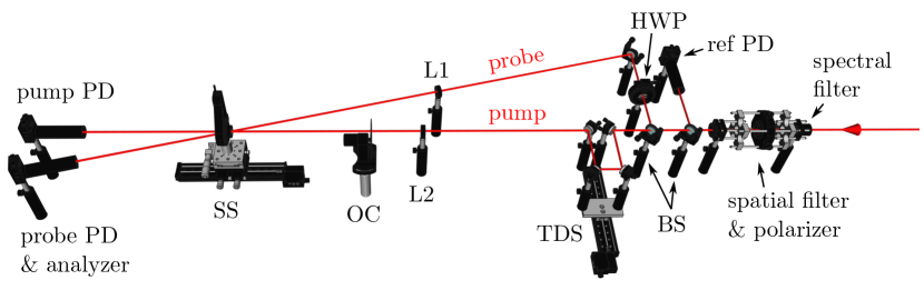
Figure 1: PPMS experimental setup. The beam passes through spectral and spatial filters and a thin-film polarizer. The first of two beam splitters (BS) picks off a reference beam by reflecting 4% to the reference photodiode detector (ref PD). A second pellicle beam splitter (BS) transmits 90% (pump) and reflects 10% (probe). A time delay stage (TDS) controls the relative time delay between the pump and probe pulses, and a half-wave plate (HWP) controls the relative probe polarization. The beams are focused by lenses (L1 and L2), and the pump beam is modulated with an optical chopper (OC). The beams overlap at an angle of $\sim 15^{\circ}$ on the sample which is mounted in the sample stage (SS) having fine $X$,$Z$-translation, 2-axis rotation, and tip-tilt control. The transmitted beams are detected with photodiode detectors (PD). Image includes CAD models courtesy of Thorlabs Inc., Zaber Technologies Inc., and Edmund Optics Inc. All rights reserved.

III.1.2 Pump and probe spatiotemporal profiles

The pulse duration was measured by performing a SHG second-order autocorrelation. Pump power was measured with a Coherent FieldMate Si photodiode (PD) head (650 - 1100nm) or with a reference PD calibrated with a thermal head (1200 - 2000 nm). In order to reduce sensitivity on overlap position and geometric effects, the probe radius was kept $5\times$ smaller than the pumpDiels and Rudolph (1996) (the beam waists were not at the sample plane) which necessitated attenuating the probe pulse energy with neutral density filters $\sim 250\times$ lower than the pump to keep the fluence ratio $F_{2}/F_{1}>10$. Pump and probe beams impinged on each sample at $\approx 7.5^{\circ}$ from the surface normal, and at $\approx 15^{\circ}$ with respect to each other. The latter angle became $\approx 5^{\circ}$ (i.e. approximately collinear) inside each sample after taking refraction into account. The beam radii at the overlap position were measured using an automated knife-edge technique, and measurements at $Z=\pm 10$ and $\pm 20$ mm from the overlap were used to measure the beam angles and Rayleigh ranges.

III.1.3 Samples

The samples were semi-insulating undoped n-type GaAs (110) with resistivity $\rho=1.9$ – $4.4$ E7 $\Omega$ cm, intrinsic carrier concentration $N_{c}=3.2$ – $11$ E7 cm^-3, carrier mobility $\mu=3.7$ – $4.4$ E3 cm² V^-1 s^-1, etch pitch density $EPD<6000$ cm^-2, and thickness $L=0.538\pm 0.005$ mm; undoped GaP (110) with $L=0.536\pm 0.005$ mm; and undoped Si (110) with $\rho=1$ – $10$ $\Omega$ cm and $L=0.485\pm 0.005$ mm. The spatial and temporal overlap of the beams was fine-tuned for each sample using 2PA prior to all data acquisition scans. The linear optical properties of the samples were measured using a J.A. Wollam M2000 variable-angle spectroscopic ellipsometer (VASE) and are reported in the Supplementary Material. Linear optical properties for $\lambda>1690$ nm were obtained from literature.Skauli et al. (2003); Li (1980)

III.2 Data collection and analysis procedure

III.2.1 Time delay scans

The 2PA coefficient was determined by performing a time delay scan and fitting the normalized probe transmission to Eq. 7. The fitting algorithm compared the variation in the fitting parameter $\beta_{12}^{\parallel,\perp}I_{2}^{0}L$ for the $N=1$ and $N=2$ cases, and if the variation was below a threshold of $1\%$, then the result for the $N=1$ case was reported; if the variation was larger, the process was repeated, comparing successively higher-order terms. The normalized change in probe transmission was calculated by

$$\frac{\Delta T_{1}(\Delta t)}{T_{1}}=\frac{V_{1}(\Delta t)}{\overline{V}_{1}^{cal}},$$ (30)

where $V_{1}$ is the probe lock-in amplitude during the time delay scan and $\overline{V}_{1}^{cal}$ is the mean lock-in amplitude corresponding to $100\%$ absorption when the probe is modulated by the optical chopper during a calibration scan. After fitting, $\Delta T_{1}(\Delta t)/T_{1}$ was adjusted by the vertical offset parameter which removes the effect of any scattered pump light. When multiple scans were performed at a single excitation energy, the mean value of $\beta_{12}$ was reported and the uncertainty was conservatively quantified by the maximum of the set including the standard error of the mean, the propagated uncertainty of the mean, and the propagated uncertainty in the individual measurements.

III.2.2 Rotation scans

The values of $\sigma$ and $\eta$ were determined by performing rotation scans of the sample fixed at the spatial overlap position and $\Delta t=0$ in both co-polarized and cross-polarized geometries. Power fluctations can sometimes complicate the signal, and so the magnitude of the pump-induced absorption was corrected according to

$$\beta_{12}(\theta)\sim-\bigg{(}\frac{\Delta T_{1}(\theta)}{T_{1}}\bigg{)}\bigg{(}\frac{1}{V_{ref}(\theta)}\bigg{)}$$ (31)

and

$$\frac{\Delta T_{1}(\theta)}{T_{1}}=\frac{V_{1}(\Delta t=0,\theta)-V_{1}(\Delta t\rightarrow-\infty,\theta)}{\overline{(V_{1}^{cal}/V_{ref}^{cal})}V_{ref}(\theta)-V_{1}(\Delta t\rightarrow-\infty,\theta)},$$ (32)

where $V_{ref}(\theta)$ is a reference voltage monitoring the incident power, $V_{1}(\Delta t\rightarrow-\infty)$ is the lock-in amplitude of the probe at large negative time delay (and thus negligible 2PA, capturing any offset), and $\overline{(V_{1}^{cal}/V_{ref}^{cal})}$ is the mean of the probe lock-in amplitude normalized to the reference amplitude during the calibration scan.

Zincblende semiconductors can exhibit the photorefractive effect which can lead to transient two-beam coupling.Dvorak et al. (1994) Transient energy transfer between beams propagating along the $110$-direction due to the photorefractive effect is antisymmetric about rotations of $R_{Z}(\pi)$, while 2PA is symmetric.Dvorak et al. (1994) Analyzing only the symmetric part removes any contribution from the photorefractive effect. In addition, random fluctuations are also reduced. The symmetric and antisymmetric parts of the change in probe transmission are

$$\frac{\Delta T_{1}^{\pm}(\theta)}{T_{1}}=\frac{1}{2}\bigg{[}\frac{\Delta T_{1}(\theta)}{T_{1}}\pm\frac{\Delta T_{1}(\theta+\pi)}{T_{1}}\bigg{]},$$ (33)

where $\Delta T_{1}^{+}(\theta)/T_{1}$ and $\Delta T_{1}^{-}(\theta)/T_{1}$ are the symmetric and antisymmetric parts, respectively, of the change in probe transmission upon rotations of $R_{Z}(\pi)$.

III.3 Results

III.3.1 Time delay scans

Fig. 2 (a) shows an example of a time delay scan for GaP at $\hbar\omega=1.55$ eV in co-polarized geometry. Baseline probe absorption $\Delta T/T$ returned to zero at both positive and negative delays $|\Delta t|>250$ fs, indicating negligible FCA. We observed the same symmetry in all $\Delta t$ scans presented in this study.

Figure 2: a) $\Delta T_{1}/T_{1}$ vs. $\Delta t$ for GaP at $\hbar\omega=1.55$ eV measured by PPMS in co-polarized geometry (circles) representative of a typical time delay scan. The on-axis peak pump intensity was $I_{2}^{0}=0.236\pm 0.012$ GW cm^-2 with pulse duration $\tau_{FWHM}=125\pm 2$ fs. Fitting the data (solid curve) gave a 2PA coefficient of $\beta_{12}^{\parallel}=4.7\pm 0.3$ cm GW^-1 for $N=2$ terms and FCA was negligible at $b^{\parallel}=0.0000\pm 0.0001$. b) $\Delta T_{1}/T_{1}$ vs. $\Delta t$ for GaP at $\hbar\omega=1.91$ eV measured by PPMS in co-polarized geometry (circles) showing the temporally-broadened asymmetric anomaly as $\hbar\omega\rightarrow E_{g}$. The second-order autocorrelation signal expected for 2PA is superimposed (dashed curve) for $\tau_{FWHM}=154\pm 6$ fs. c) $\Delta T_{1}/T_{1}$ vs. $\Delta t$ for GaP at $\hbar\omega=0.77$ eV measured by PPMS in co-polarized geometry (circles) showing the coherent artifact with an increase in transmission for positive time delays likely due to transient energy transfer from a nonlinear refractive index phase grating as $\hbar\omega\rightarrow E_{g}/2$.

For $|\Delta t|<250$ fs, the width of the measured 2PA response (data points) fits very closely to the calculated response (solid black curve) with the pulse duration independently measured by SHG second-order autocorrelation. We obtained a similar match for most data presented here. For a small number of exceptional cases, we observed a 2PA response slightly wider than the SHG autocorrelation. For these cases, we considered the possiblity of saturation effect and this led to a widening of error bars in reported spectra (see Supplementary Material).

In addition to revealing complete information regarding the $\mathrm{Im}\{\chi^{(3)}(\omega)\}$ tensor structure, the 2-beam PPMS technique offers another advantage over single-beam techniques in its ability to discern anomalous effects from 2PA. Such effects include FCA, transient energy transfer originating from photorefractive phase gratings, nonlinear refractive index phase gratings, 2PA amplitude gratings, free-carrier gratings, and saturable absorption which can couple the two beams.Smirl et al. (1988); Valley and Smirl (1988)

The temporal width of the nonlinear loss was anomalously broadened in GaAs and GaP as the excitation neared their respective band gaps in both polarization geometries. Fig. 2 (b) shows this anomaly in GaP at $\hbar\omega=1.91$ eV (0.85$E_{g}$) and it was also observed in GaAs at $\hbar\omega=1.38$ eV (0.96$E_{g}$). Pump depletion by pump-pump 2PA cannot account for this effect. The observed temporal FWHM in the nonlinear loss was a factor of 2.3 – 3 greater than expected for 2PA alone. Asymmetry in the time delay scans also supports the presence of other effects not accounted for in our model. Both of these features are obvious against the second-order autocorrelation signal expected for 2PA (as measured by SHG) which is superimposed on the data.

A fs-scale time delay-dependent FCA cross-section could produce such an anomaly as free carriers excited predominantly by pump-pump 2PA diffuse through $k$-space in the conduction band. Zero time delay in this experiment was determined by a fit parameter, but the peak could be shifted towards positive time delays as a result of this effect. Another possibility is that a photorefractive index grating could induce transient energy transfer and generate the observed anomaly. Both of these effects are encompassed more generally by any non-instantaneous response or memory effect as the 2PA process approaches resonance. If such an effect is present it can induce a polarization density responsive not only to the instantaneous value of the electric field but also to its history on fs timescales.Diels and Rudolph (1996) Measurements at different crystal orientations, pulse energies, pulse durations, and a nondegenerate two-photon absorption experimentFishman et al. (2011); Hutchings and Stryland (1992); Bolger et al. (1993); Hannes et al. (2019) could reveal more information about the nature of such anomalies.

Below the two-photon absorption band edge of GaAs and GaP, nonlinear loss was very small except at high intensities (a factor of 1 – 20 greater than intensities at excitation energies $\hbar\omega>E_{g}/2$). This is consistent with 2PA being energetically disallowed but a transient coherent artifactLebedev et al. (2005) was still observed near zero time delay in both polarization geometries. A transient coherent artifact was also observed in Si near to but slightly above $E_{g}/2$ at $\hbar\omega=0.62$ eV, where the magnitude of 2PA was also quite low. This coherent artifact was asymmetric and notably included an antisymmetric component (about $\Delta t=0$) where $\Delta T_{1}/T_{1}>0$ briefly for positive time delays. While $\mathrm{Im}\{\chi^{(3)}(\omega)\}\rightarrow 0$ rapidly at the two-photon band edge, $\mathrm{Re}\{\chi^{(3)}(\omega)\}$ in general does not. $\mathrm{Re}\{\chi^{(3)}(\omega)\}$ encodes the nonlinear refractive index which is related to $\mathrm{Im}\{\chi^{(3)}(\omega)\}$ by nonlinear Kramers-Kronig relations.Boyd (2008) Below resonance, $\mathrm{Re}\{\chi^{(3)}(\omega)\}\sim\omega^{-3}$ in semiconductors and thus is the dominant third-order nonlinearity at low excitation energies.Boyd (2008)

This coherent artifact shown in Fig. 2 (c) likely arises from a nonlinear refractive index phase grating, which can transfer energy between the probe and pump and produce such antisymmetric time delay profiles.Palfrey and Heinz (1985) This effect is a background effect that likely occurs in all measurements, but is so weak that it is only visible when 2PA is no longer the dominant third-order nonlinearity.

III.3.2 2PA spectra

The 2PA spectrum for GaAs measured by PPMS in co-polarized geometry is shown in Fig. 3 along with the fit using the Jones-Reiss model in Eq. 27, published values using mostly single-beam techniques, and ab initio calculations. The best fit of this data to the Jones-Reiss model gives $B=510\pm 210$ cm GW^-1 and a 2PA peak of $\beta^{JR}_{max}=24\pm 10$ cm GW^-1. The 2PA coefficient reported in literature has a large spread, mainly from single-beam experiments clustered around 1053 nm using picosecond lasers.

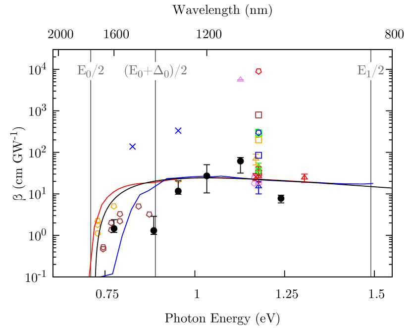
Figure 3: 2PA coefficient ($\beta=\frac{1}{2}\beta_{12}^{\parallel}$) spectrum of GaAs measured by PPMS in co-polarized geometry for $E_{g}/2<\hbar\omega<E_{g}$ (solid black circles). The best fit of this data to the Jones-Reiss model is shown with the black curve. Data from a two-beam experiment is shown with a red triangleDvorak et al. (1994). Data from other sources using single-beam experiments are also shown; blue triangleBosacchi, Bessey, and Jain (1978), green trianglePenzkofer and Bugayev (1989), orange triangleSaissy et al. (1978), violet triangleJayaraman and Lee (1972), brown triangleBechtel and Smith (1976), red squareKleinman, Miller, and Nordland (1973), blue squareBepko (1975), green squareLee and Fan (1974), orange squareOksman et al. (1972), violet squareRalston and Chang (1969), brown squareArsenev et al. (1969), red pentagonBasov et al. (1966), blue pentagonGrasyuk et al. (1973), green pentagonZubarev, Mironov, and Mikhailov (1977), orange pentagonsHurlbut et al. (2007), violet pentagonsDeSalvo et al. (1993), brown pentagonsFishman et al. (2011), red XSaid et al. (1992), and blue X’sZhi-hui et al. (2015). Theoretical calculations from Hutchings, et al.Hutchings and Stryland (1992) are shown with the red curve, and ab initio calculations from Murayama, et al.Murayama and Nakayama (1995) are shown with the blue curve. Critical point energies are marked with gray vertical lines.Lautenschlager et al. (1987a)

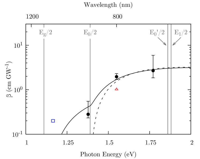
Figure 4: 2PA coefficient ($\beta=\frac{1}{2}\beta_{12}^{\parallel}$) spectrum of GaP measured by PPMS in co-polarized geometry for $E_{g}/2<\hbar\omega<E_{g}$ (solid black circles). The best fit of this data to the cumulative model is shown with the solid curve and the Jones-Reiss model for direct transitions with the dashed curve. Data from other sources using single-beam experiments are also shown; red triangleHoffman and Mott (2012) and blue squareBechtel and Smith (1976). Critical point energies are marked with gray vertical lines.Zallen and Paul (1964)

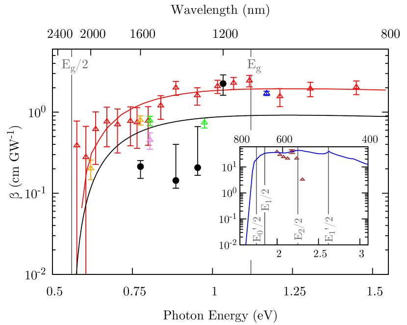
Figure 5: 2PA coefficient ($\beta=\frac{1}{2}\beta_{12}^{\parallel}$) spectrum of Si measured by PPMS in co-polarized geometry for $E_{g}/2<\hbar\omega<E_{g}$ (solid black circles). The best fit of this data to the Garcia-Kalyanaraman model is shown with the black curve and the fit to the data from Bristow, et al.Bristow, Rotenberg, and van Driel (2007) is shown with the red curve and red triangles, respectively. Data from other sources using single-beam experiments are also shown; blue triangleReintjes and McGroddy (1973), green trianglesDinu, Quochi, and Garcia (2003), orange trianglesEuser and Vos (2005), and violet triangleTsang et al. (2002). Inset: Data from a two-beam experiment above the direct two-photon band gap is shown with brown trianglesReitze et al. (1990) and ab initio calculations from Murayama, et al.Murayama and Nakayama (1995) are shown with the blue curve. Critical point energies are marked with gray vertical lines.Murayama and Nakayama (1995); Lautenschlager et al. (1987b)

The 2PA spectrum for GaP measured by PPMS in co-polarized geometry is shown in Fig. 4 along with a fit using a cumulative model for direct and indirect transitions, a fit using the Jones-Reiss model for direct transitions near $E_{0}/2$, and a comparison to published values using single-beam techniques. The cumulative model is defined as using the Garcia-Kalyanaraman model for $E_{g}/2\leq\hbar\omega<E_{0}/2$, and a sum of this function and the Jones-Reiss model above $E_{0}/2$. The best fit to this model gives $B=44\pm 18$ cm GW^-1 and $C=49\pm 35$ cm GW^-1, with 2PA contributions peaking at $\beta^{GK}_{max}=1.1\pm 0.8$ cm GW^-1 for indirect transitions and $\beta^{JR}_{max}=2.1\pm 0.9$ cm GW^-1 for direct transitions.

The 2PA spectrum for Si measured by PPMS in co-polarized geometry is shown in Fig. 5 along with the fit using the Garcia-Kalyanaraman model and a comparison to published values using single-beam techniques. The best fit of this data to the Garcia-Kalyanaraman model gives $C=41\pm 25$ cm GW^-1, peaking at $\beta^{GK}_{max}=0.9\pm 0.6$ cm GW^-1, which is considerably lower than the fit to the data from Bristow, et al.Bristow, Rotenberg, and van Driel (2007) of $C=86$ cm GW^-1, peaking at $\beta^{GK}_{max}=1.93$ cm GW^-1. The measured dispersion differs from the phenomenological model. These results are tabulated in the Supplementary Material. An inset in Fig. 5 shows the degenerate 2PA spectrum predicted by ab initio calculations valid above $E_{0}^{\prime}/2=1.75$ eV and published values using a two-beam technique.

III.3.3 Rotation scans

An example of a rotation scan for GaP at $\hbar\omega=1.55$ eV showing symmetric and antisymmetric parts of the normalized $-\Delta T_{1}(\theta)/T_{1}$ in co- and cross-polarized geometries is shown in Fig. 6. The fits of the co- and cross-polarized symmetric data share global parameters $\sigma$ and $\theta_{0}$, while the other parameters are independent. The antisymmetric part is typically $<10\%$ of the magnitude of the symmetric part.

Figure 6: $-\Delta T_{1}^{+}/T_{1}$ vs. $\theta$ for GaP at $\hbar\omega=1.55$ eV in a) co-polarized and b) cross-polarized geometries. The resulting fits (solid curves) are shown and give $\sigma=-0.86\pm 0.07$, $\eta=0.18\pm 0.18$, and $\theta_{0}=132.2^{\circ}\pm 1.0^{\circ}$ (describing the relative orientation of lab $X$-axis from $\overline{1}10$ crystal direction). The antisymmetric part $-\Delta T_{1}^{-}/T_{1}$ vs. $\theta$ in c) co-polarized and d) cross-polarized geometries.

III.3.4 Anisotropy spectra

The spectra of anisotropy and dichroism parameters for GaAs, GaP, and Si are reported in Table 2, along with the calculations of the relative amplitudes of $\mathrm{Im}\{\chi^{(3)}_{xxyy}\}$ and $\mathrm{Im}\{\chi^{(3)}_{xyyx}\}$ to $\mathrm{Im}\{\chi^{(3)}_{xxxx}\}$. The values of $\sigma$ from this work are compared to the range of theoretical predictions of $\sigma$ for GaAs and GaP from Table 1 as well as results reported in literature for GaAs and Si. $|\sigma|$ is largest for GaP, which is consistent with theoretical predictions at the two-photon band edge. The values of $\eta$ from this work are compared to a previously reported value in literature for GaAs, and ab initio calculations for anisotropy in GaAs are also shown. See the Supplementary Material for additional information on comparing values between different sources in literature.

Table 2: Measured spectra of 2PA anisotropy and dichroism parameters for GaAs, GaP, and Si. The relative values of $\mathrm{Im}\{\chi^{(3)}_{xxyy}\}/\mathrm{Im}\{\chi^{(3)}_{xxxx}\}=\big{[}1-(\sigma+\eta)\big{]}/2=\big{[}2-(\sigma+2\delta)\big{]}/2$ and $\mathrm{Im}\{\chi^{(3)}_{xyyx}\}/\mathrm{Im}\{\chi^{(3)}_{xxxx}\}=\eta=(2\delta-\sigma)/2$ are also tabulated. Literature and theoretical values are included and referenced in Notes. See Table 1 for derivations of theoretical values.

Sample	$\hbar\omega$ (eV)	$\sigma$	$\delta\sigma$	$\delta$	$\delta(\delta)$	$\frac{\mathrm{Im}\{\chi^{(3)}_{xxyy}\}}{\mathrm{Im}\{\chi^{(3)}_{xxxx}\}}$	$\delta\frac{\mathrm{Im}\{\chi^{(3)}_{xxyy}\}}{\mathrm{Im}\{\chi^{(3)}_{xxxx}\}}$	$\frac{\mathrm{Im}\{\chi^{(3)}_{xyyx}\}}{\mathrm{Im}\{\chi^{(3)}_{xxxx}\}}$	$\delta\frac{\mathrm{Im}\{\chi^{(3)}_{xyyx}\}}{\mathrm{Im}\{\chi^{(3)}_{xxxx}\}}$	Notes
GaAs	0.72	-0.38								Theoretical: see Table 1
	0.72	-0.45								Theoretical: see Table 1
	0.72	-0.68								Theoretical: see Table 1
	0.77	-0.13	0.08	0.68	0.17	0.20	0.13	0.74	0.17
	0.88	-0.65		-0.50		0.91		-0.17		Ab initio: Murayama, et al.Murayama and Nakayama (1995)
	0.89	-0.36	0.06	0.0	0.3	0.58	0.18	0.2	0.3
	0.93	-0.46		-0.01		0.62		0.22		Ab initio: Murayama, et al.Murayama and Nakayama (1995)
	0.95	-0.29	0.05	0.47	0.11	0.34	0.08	0.61	0.10
	0.95	-0.56		0.02		0.63		0.29		Ab initio: Murayama, et al.Murayama and Nakayama (1995)
	1.03	-0.27	0.08	0.4	1.6	0.4	0.8	0.5	1.6
	1.03	-0.47		0.15		0.54		0.39		Ab initio: Murayama, et al.Murayama and Nakayama (1995)
	1.13	-0.40	0.05	0.42	0.12	0.39	0.07	0.62	0.09
	1.13	-0.58		0.26		0.51		0.55		Ab initio: Murayama, et al.Murayama and Nakayama (1995)
	1.17	-0.224	0.011							Bepko, et al.Bepko (1975)
	1.17	-0.3								Bechtel, et al.Bechtel and Smith (1976)
	1.17	-0.74	0.18							DeSalvo, et al.DeSalvo et al. (1993)
	1.17	0.00	0.15							Said, et al.Said et al. (1992)
	1.17	-0.57		0.28		0.50		0.55		Ab initio: Murayama, et al.Murayama and Nakayama (1995)
	1.23	-0.64		0.29		0.51		0.61		Ab initio: Murayama, et al.Murayama and Nakayama (1995)
	1.24	-0.23	0.05	0.64	0.01	0.24	0.06	0.75	0.07
	1.31	-0.76	0.08	0.22	0.24	0.58	0.08	0.60	0.20	Dvorak, et al.Dvorak et al. (1994)
	1.31	-0.64		0.34		0.49		0.66		Ab initio: Murayama, et al.Murayama and Nakayama (1995)
	1.48	-0.66		0.34		0.49		0.67		Ab initio: Murayama, et al.Murayama and Nakayama (1995)
GaP	1.38	-0.53	0.06	0.09	0.17	0.59	0.10	0.35	0.14
	1.39	-0.85								Theoretical: see Table 1
	1.39	-1.06								Theoretical: see Table 1
	1.39	-1.59								Theoretical: see Table 1
	1.55	-0.88	0.10	-0.13	0.23	0.79	0.14	0.31	0.18
	1.77	-0.61	0.09	0.1	0.7	0.6	0.3	0.4	0.6
Si	0.58	0.00	0.05							Bristow, et al.Bristow, Rotenberg, and van Driel (2007)
	0.77	-0.55	0.09	0.1	0.4	0.60	0.20	0.4	0.3
	0.89	-0.03	0.04	0.95	0.08	0.04	0.05	0.96	0.06
	0.89	0.00	0.05							Bristow, et al.Bristow, Rotenberg, and van Driel (2007)
	0.95	-0.15	0.14	0.77	0.23	0.16	0.15	0.84	0.16
	1.03	-0.29	0.08	0.2	0.6	0.5	0.3	0.3	0.6
	1.65	-0.08		0.50		0.18		0.54		Ab initio: Murayama, et al.Murayama and Nakayama (1995)

IV Discussion

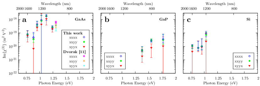
Figure 7: $\mathrm{Im}\{\chi^{(3)}(\omega)\}$ tensor spectrum obtained by 2PA PPMS time delay and anisotropy measurements for a) GaAs, b) GaP, and c) Si. Previously reported values for GaAs at $\hbar\omega=1.31$ eV by Dvorak, et al.Dvorak et al. (1994) are indicated. The values are tabulated in the Supplementary Material.

The complete set of measurements performed ranged from 0.62 – 1.38 eV for GaAs, 0.77 – 1.91 eV for GaP, and 0.62 – 1.03 eV for Si. Long-lifetime time-independent FCA was observed to be negligible in the regime studied in this work as evidenced by the complete recovery of the transmission of the probe at sufficiently large positive time delays. The antisymmetric part of $\Delta T_{1}/T_{1}$ in the rotation scans was generally small in comparison to the symmetric part, and thus the photorefractive effect did not significantly affect the anisotropy measurements in the regime studied. However, other anomalies were observed within this range for which the model for 2PA considered in this work was unable to explain, as detailed in Section III.3.1. The anomaly observed in time delay scans characterized by asymmetric temporal broadening and strong nonlinear loss precluded an estimation of $\beta$ at 1.38 eV for GaAs and 1.91 eV for GaP, near their respective band gaps. This anomaly indicated the presence of a transient effect of the pump on the probe which depended on the history of the incident field. A distinctly different anomaly was observed in time delay scans characterized by an antisymmetric component with an increase in probe transmission for positive delays for which the likely source was a nonlinear refractive index phase grating. This precluded an estimation of $\beta$ at 0.62 – 0.69 eV for GaAs, 0.77 – 1.24 eV for GaP, and 0.62 – 0.69 eV for Si, near their respective two-photon band edges. The co-polarized rotation scans often did not follow the expected form of 2PA for $\overline{4}3m$ or $m3m$ crystal symmetry when the antisymmetric time delay scan anomaly was observed. However, some of the rotation scans did still match the expected form even with the presence of a time delay scan anomaly which suggests that 2PA may still be dominant at zero time delays. The complete set of measurements is outlined in the Supplementary Material. The 2PA spectra presented here reflect only the data for which no anomaly was observed.

The dispersion observed in GaAs in Fig. 3 indicates that the spectral structure of 2PA is more complex than predicted by the Jones-Reiss model. The peak in 2PA measured at 1.13 eV is close to that expected from the Jones-Reiss model of 1.03 eV. The measured spectra is comparable in magnitude to ab initio calculations. The number of surviving spectral measurements of $\beta$ in GaP and Si are too few to make compelling statements about the agreement with phenomenological models, but this also illustrates the importance of identifying anomalous responses not attributable to 2PA which is often only possible with a 2-beam experiment. Measurements of 2PA in GaP at increased spectral density near $E_{0}/2$ could better constrain the relative strengths of direct and indirect two-photon transitions. 2PA in Si between $E_{g}/2=0.56$ eV and $E_{0}^{\prime}/2=1.75$ eV is due to either phonon-mediated transitions or transitions involving defect or dopant states. Measurements of the degenerate 2PA spectrum dependence on temperature in this spectral range could verify the relative contributions to 2PA by these two mechanisms. The ab initio calculations of 2PA in Si by Murayama, et al. consider only direct transitions and thus are applicable in describing 2PA above $E_{0}^{\prime}/2$.Murayama and Nakayama (1995)

The parameters $\beta_{12}(\omega)$, $\sigma(\omega)$, and $\eta(\omega)$ characterize the three independent components $\mathrm{Im}\{\chi^{(3)}_{xxxx}(\omega)\}$, $\mathrm{Im}\{\chi^{(3)}_{xxyy}(\omega)\}$, and $\mathrm{Im}\{\chi^{(3)}_{xyyx}(\omega)\}$. The relative amplitudes of the off-diagonal tensor components to the $\mathrm{Im}\{\chi^{(3)}_{xxxx}\}$ component are shown in Table 2, and the absolute amplitude of the $\mathrm{Im}\{\chi^{(3)}_{abcd}(\omega)\}$ tensor spectra for GaAs, GaP, and Si are shown in Fig. 7 and compared with results from literature for GaAs.Dvorak et al. (1994) See the Supplementary Material for more information on comparing values of the tensor components to literature results. The relative amplitudes of the tensor components $\mathrm{Im}\{\chi^{(3)}_{xxyy}(\omega)\}/\mathrm{Im}\{\chi^{(3)}_{xxxx}(\omega)\}$ differ by more than their uncertainties for all samples and excitation energies except for GaAs at $\hbar\omega=1.03$ eV, where the anisotropy was only weakly constrained. The relative amplitudes of $\mathrm{Im}\{\chi^{(3)}_{xyyx}(\omega)\}/\mathrm{Im}\{\chi^{(3)}_{xxxx}\}$ also differ by more than their uncertainties for all samples and excitation energies except for GaAs at $\hbar\omega=1.03$ eV again, and also for GaP at $\hbar\omega=1.77$ eV, and Si at $\hbar\omega=0.89$ and 0.95 eV. The relative amplitudes $\mathrm{Im}\{\chi^{(3)}_{xyyx}(\omega)\}/\mathrm{Im}\{\chi^{(3)}_{xxyy}(\omega)\}$ differ by more than their uncertainties for GaAs at $\hbar\omega=0.77$, 0.95, 1.13, and 1.24 eV, for GaP at $\hbar\omega=1.55$ eV, and for Si at $\hbar\omega=0.89$ and 0.95 eV. Thus Kleinman symmetry is broken, a feature not discerned in the result from Dvorak, et al. for GaAs at 1.31 eV.Dvorak et al. (1994) Indeed, Kleinman symmetry should be broken in the presence of dispersion in $\mathrm{Im}\{\chi^{(3)}(\omega)\}$.Kleinman (1962); Boyd (2008)

V Conclusions

We characterized the $\mathrm{Im}\{\chi^{(3)}_{abcd}(\omega)\}$ tensor spectrum by measuring the degenerate two-photon absorption coefficient and its anisotropy using a 2-beam PPMS experiment for bulk 110-cut GaAs, GaP, and Si at 300 K over an overall excitation range $0.62<\hbar\omega<1.91$ eV ($650<\lambda<2000$ nm). The phenomenological 2PA dispersion models we used qualitatitvely agree with our experimental results for GaAs and GaP but there remain significant discrepancies, especially in Si. These could be due to the models lacking consideration of the full band structure of these materials including the effect of anisotropy or additional nonlinear effects. Ab initio calculations in GaAs roughly agree with the observed dispersion. We observed an anomalous asymmetric temporally-broadened nonlinear loss in GaAs and GaP when $\hbar\omega$ approached their respective band gaps which could be due to a variety of noninstantaneous nonlinear responses. We also observed a coherent artifact in all three samples near $E_{g}/2$ which was likely due to a nonlinear refractive index phase grating. Kleinman symmetry was observed to be broken in all three materials.

Our results motivate further development of ab initio theoriesStryland et al. (1985); Bechstedt, Adolph, and Schmidt (1999); Attaccalite and Grüning (2013); Grüning and Attaccalite (2020); Murayama and Nakayama (1995) such as those which use DFT in the length gauge,Anderson et al. (2015, 2016); Anderson (2016); Anderson and Mendoza (2016) and experimental measurements of the degenerate 2PA spectrum dependence on temperature in Si and GaP which could help elucidate the potential contributions to 2PA below the two-photon direct-gap. Experiments at higher spectral density, using nondegenerate beams, and investigating a larger range of pulse energy- or duration-dependence could identify other nonlinear effects that may be present in these materials at femtosecond timescales. If phonon-mediated transitions are indeed dominant below the two-photon direct-gap in indirect band gap semiconductors, this would motivate further development of ab initio calculations of the $\mathrm{Im}\{\chi^{(3)}_{abcd}(\omega)\}$ tensor spectra which account for such transitions.Noffsinger et al. (2012)

Data Availability

The data that supports the findings of this study are available within the article and its supplementary material, and additional information that support the findings of this study are available from the corresponding author upon reasonable request.

References

References

- Asghari and Krishnamoorthy (2011) M. Asghari and A. Krishnamoorthy, Nat. Photonics 5, 268–270 (2011).
- Yoon et al. (2010) J. Yoon, S. Jo, I. Chun, I. Jung, H. Kim, M. Meitl, E. Menard, X. Li, J. Coleman, U. Paik, and J. Rogers, Nature 465, 329–333 (2010).
- Bett et al. (1999) A. Bett, F. Dimroth, G. Stollwerck, and O. Sulima, Appl. Phys. A 69, 119–129 (1999).
- Wada (1988) O. Wada, Opt. Quantum Electron. 20, 441–474 (1988).
- Pilkuhn and Foster (1966) M. Pilkuhn and L. Foster, IBM J. Res. Dev. 10, 122–129 (1966).
- Wilson et al. (2020) D. Wilson, K. Schneider, S. Hönl, M. Anderson, Y. Baumgartner, L. Czornomaz, T. Kippenberg, and P. Seidler, Nat. Photonics 14, 57–62 (2020).
- Euser and Vos (2005) T. Euser and W. Vos, J. Appl. Phys. 97, 043102 (2005).
- Vlasov et al. (2001) Y. Vlasov, X. Bo, J. Sturm, and D. Norris, Nature 414, 289–293 (2001).
- Rong et al. (2005) H. Rong, A. Liu, R. Jones, O. Cohen, D. Hak, R. Nicolescu, A. Fang, and M. Paniccia, Nature 433, 725–728 (2005).
- Tsang et al. (2002) H. Tsang, C. Wong, T. Liang, I. Day, S. Roberts, A. Harpin, J. Drake, and M. Asghari, Appl. Phys. Lett. 80, 416–418 (2002).
- Dvorak et al. (1994) M. Dvorak, W. Schroeder, D. Andersen, A. Smirl, and B. Wherrett, IEEE J. Quantum Electron. 30, 256–268 (1994).
- Blanco et al. (2000) A. Blanco, E. Chomski, S. Grabtchak, M. Ibisate, S. John, S. Leonard, C. Lopez, F. Meseguer, H. Miguez, J. Mondia, G. Ozin, O. Toader, and H. van Driel, Nature 405, 437–440 (2000).
- Bristow, Rotenberg, and van Driel (2007) A. Bristow, N. Rotenberg, and H. van Driel, Appl. Phys. Lett. 90, 191104 (2007).
- Bassani and Scandolo (1991) F. Bassani and S. Scandolo, Phys. Rev. B 44, 8446–8453 (1991).
- Caspers (1964) P. Caspers, Phys. Rev. A 133, 1249 (1964).
- Hutchings et al. (1992) D. Hutchings, M. Sheik-Bahae, D. Hagan, and E. V. Stryland, Opt. Quantum Electron. 24, 1–30 (1992).
- Kogan (1963) S. Kogan, Sov. Phys. JETP 16, 217 (1963).
- Gibbs (1972) H. Gibbs, Causality and Dispersion Relations (Academic Press, New York, 1972).
- Price (1964) P. Price, Phys. Rev. 130, 1792 (1964).
- Jr. and Jr. (1975) F. R. Jr. and R. G. Jr., Phys. Rev. B 11, 2768 (1975).
- Sheik-Bahae, Hagan, and Styland (1990) M. Sheik-Bahae, D. Hagan, and E. V. Styland, Phys. Rev. Lett. 65, 96–99 (1990).
- Sheik-Bahae et al. (1991) M. Sheik-Bahae, D. Hutchings, D. Hagan, and E. V. Stryland, IEEE J. Quantum Electron. 27, 1296–1309 (1991).
- Toll (1956) J. Toll, Phys. Rev. 104, 1760 (1956).
- Gibbs (1985) H. Gibbs, Optical Bistability: Controlling Light with Light (Academic Press, Orlando, 1985).
- Stegeman and Wright (1990) G. Stegeman and E. Wright, Opt. Quantum Electron. 22, 95–122 (1990).
- Reintjes and McGroddy (1973) J. Reintjes and J. McGroddy, Phys. Rev. Lett. 30, 901–903 (1973).
- Bechtel and Smith (1976) J. Bechtel and W. Smith, Phys. Rev. B 13, 3515–3522 (1976).
- Bosacchi, Bessey, and Jain (1978) B. Bosacchi, J. Bessey, and F. Jain, J. Appl. Phys. 49, 4609–4611 (1978).
- Stryland et al. (1994) E. V. Stryland, M. Sheik-Bahae, T. Xia, C. Wamsley, Z. Wang, A. Said, and D. Hagan, Int. J. Nonlinear Opt. Phys. 3, 489–500 (1994).
- Sheik-Bahae and Stryland (1999) M. Sheik-Bahae and E. V. Stryland, Semiconductors and Semimetals, edited by R. Willardson and E. Weber, Vol. 58 (Academic Press, San Diego, 1999) pp. 257–318.
- Reitze et al. (1990) D. Reitze, T. Zhang, W. Wood, and M. Downer, J. Opt. Soc. Am. B 7, 84–89 (1990).
- Hurlbut et al. (2007) W. Hurlbut, Y. Lee, K. Vodopyanov, P. Kuo, and M. Fejer, Opt. Lett. 32, 668–670 (2007).
- Fishman et al. (2011) D. Fishman, C. Cirloganu, S. Webster, L. Padilha, M. Monroe, D. Hagan, and E. V. Stryland, Nat. Photonics 5, 561–565 (2011).
- Shank, Ippen, and Shapiro (1978) C. Shank, E. Ippen, and S. Shapiro, eds., Picosecond Phenomena (Springer-Verlag, Hilton Head, 1978).
- Benis et al. (2020) S. Benis, C. Cirloganu, N. Cox, T. Ensley, H. Hu, G. Nootz, P. Olszak, L. Padilha, D. Peceli, M. Reichert, S. Webster, M. Woodall, D. Hagan, and E. V. Stryland, Optica 7, 888–899 (2020).
- Cirloganu (2010) C. Cirloganu, Experimental And Theoretical Approaches To Characterization Of Electronic Nonlinearities In Direct–gap Semiconductors, Ph.D. thesis, University of Central Florida (2010).
- Boyd (2008) R. Boyd, Nonlinear Optics, 3rd ed. (Academic Press - Elsevier, Inc., Burlington, 2008).
- Popov, Svirko, and Zheludev (1995) S. Popov, Y. Svirko, and N. Zheludev, Susceptibility Tensors for Nonlinear Optics, Optics and Optoelectronics Series (Institute of Physics Publishing, Bristol, 1995).
- Kleinman (1962) D. Kleinman, Phys. Rev. 126, 1977 (1962).
- Murayama and Nakayama (1995) M. Murayama and T. Nakayama, Phys. Rev. B 52, 4986–4997 (1995).
- Noffsinger et al. (2012) J. Noffsinger, E. Kioupakis, C. V. de Welle, S. Louie, and M. Cohen, Phys. Rev. Lett. 108, 167402–167407 (2012).
- Jones and Reiss (1977) H. Jones and H. Reiss, Phys. Rev. B 16, 2466–2473 (1977).
- Wherrett (1984) B. Wherrett, J. Opt. Soc. Am. B 1, 67–72 (1984).
- Garcia and Kalyanaraman (2006) H. Garcia and R. Kalyanaraman, J. Phys. B 39, 2737–2746 (2006).
- Garcia (2006) H. Garcia, Phys. Rev. B 74, 035212 (2006).
- Aspnes (1972) D. Aspnes, Phys. Rev. B 6, 4648–4659 (1972).
- Moss, Sipe, and van Driel (1987) D. Moss, J. Sipe, and H. van Driel, Phys. Rev. B 36, 9708–9721 (1987).
- Zallen and Paul (1964) R. Zallen and W. Paul, Phys. Rev. 134, A1628–A1641 (1964).
- Diels and Rudolph (1996) J. Diels and W. Rudolph, Ultrafaser Laser Pulse Phenomena: Fundamentals, Techniques, and Applications on a Femtosecond Time Scale (Academic Press, San Diego, 1996).
- Skauli et al. (2003) T. Skauli, P. Kuo, K. Vodopyanov, T. Pinguet, O. Levi, L. Eyres, J. Harris, M. Fejer, B. Gerard, L. Becouarn, and E. Lallier, J. Appl. Phys. 94, 6447–6455 (2003).
- Li (1980) H. Li, J. Phys. Chem. Ref. Data 9, 561–658 (1980).
- Smirl et al. (1988) A. Smirl, G. Valley, K. Bohnert, and J. T.F. Boggess, IEEE J. Quantum Electron. 24, 289–303 (1988).
- Valley and Smirl (1988) G. Valley and A. Smirl, IEEE J. Quantum Electron. 24, 304–310 (1988).
- Hutchings and Stryland (1992) D. Hutchings and E. V. Stryland, J. Opt. Soc. Am. B 9, 2065–2074 (1992).
- Bolger et al. (1993) J. Bolger, A. Kar, B. Wherrett, R. DeSalvo, D. Hutchings, and D. Hagan, Optics Commun. 97, 203 (1993).
- Hannes et al. (2019) W.-R. Hannes, L. Krauß-Kodytek, C. Ruppert, M. Betz, and T. Meier, in Ultrafast Phenomena and Nanophotonics XXIII, Vol. 10916, edited by M. Betz and A. Elezzabi, International Society for Optics and Photonics (SPIE, 2019) pp. 52–62.
- Lebedev et al. (2005) M. Lebedev, O. Misochko, T. Dekorsky, and N. Georgiev, J. Exp. Theor. Phys. 100, 272–282 (2005).
- Palfrey and Heinz (1985) S. Palfrey and T. Heinz, J. Opt. Soc. Am. B 2, 674–679 (1985).
- Penzkofer and Bugayev (1989) A. Penzkofer and A. Bugayev, Opt. Quantum Electron. 21, 283–306 (1989).
- Saissy et al. (1978) A. Saissy, A. Azema, J. Botineau, and F. Gires, Appl. Phys. 15, 99–102 (1978).
- Jayaraman and Lee (1972) S. Jayaraman and C. Lee, Appl. Phys. Lett. 20, 392–395 (1972).
- Kleinman, Miller, and Nordland (1973) D. Kleinman, R. Miller, and W. Nordland, Appl. Phys. Lett. 23, 243–244 (1973).
- Bepko (1975) S. Bepko, Phys. Rev. B 12, 669–672 (1975).
- Lee and Fan (1974) C. Lee and H. Fan, Phys. Rev. B 9, 3502–3516 (1974).
- Oksman et al. (1972) Y. Oksman, A. Semenov, V. Smirnov, and O. Smirnov, Sov. Phys. Semicond. 6, 629 (1972).
- Ralston and Chang (1969) J. Ralston and R. Chang, Appl. Phys. Lett. 15, 164–166 (1969).
- Arsenev et al. (1969) V. Arsenev, V. Dneprovskii, D. Klyshko, and A. Penin, Sov. Phys. JETP 29, 413–415 (1969).
- Basov et al. (1966) N. Basov, A. Grasiuk, I. Zubarev, V. Katulin, and O. Krokhin, Sov. Phys. JETP 23, 366 (1966).
- Grasyuk et al. (1973) A. Grasyuk, I. Zubarev, V. Lobko, Y. Matveets, A. Mironov, and O. Shatberashvili, JETP Lett. 17, 416–418 (1973).
- Zubarev, Mironov, and Mikhailov (1977) I. Zubarev, A. Mironov, and S. Mikhailov, Sov. Phys. Semicond. 11, 239 (1977).
- DeSalvo et al. (1993) R. DeSalvo, M. Sheik-Bahae, A. Said, D. Hagan, and E. V. Stryland, Opt. Lett. 18, 194–196 (1993).
- Said et al. (1992) A. Said, M. Sheik-Bahae, D. Hagan, T. Wei, J. Wang, J. Young, and E. V. Stryland, J. Opt. Soc. Am. B 9, 405–414 (1992).
- Zhi-hui et al. (2015) C. Zhi-hui, X. Si, H. Jun, and G. Bing, Chinese J. Lumin. 36, 969–975 (2015).
- Lautenschlager et al. (1987a) P. Lautenschlager, M. Garriga, S. Logothetidis, and M. Cardona, Phys. Rev. B 35, 9174–9189 (1987a).
- Hoffman and Mott (2012) R. Hoffman and A. Mott, Army Research Laboratory ARL-TR-6157 (2012).
- Dinu, Quochi, and Garcia (2003) M. Dinu, F. Quochi, and H. Garcia, Appl. Phys. Lett. 82, 2954–2956 (2003).
- Lautenschlager et al. (1987b) P. Lautenschlager, M. Garriga, L. Vina, and M. Cardona, Phys. Rev. B 36, 4821–4830 (1987b).
- Stryland et al. (1985) E. V. Stryland, M. Woodall, H. Vanherzeele, and M. Soileau, Opt. Lett. 10, 490 (1985).
- Bechstedt, Adolph, and Schmidt (1999) F. Bechstedt, B. Adolph, and W. Schmidt, Braz. J. Phys. 29, 643–651 (1999).
- Attaccalite and Grüning (2013) C. Attaccalite and M. Grüning, Phys. Rev. B 88, 235113 (2013).
- Grüning and Attaccalite (2020) M. Grüning and C. Attaccalite, “Nonlinear optics from first-principles real-time approaches,” (2020), APS March Meeting.
- Anderson et al. (2015) S. Anderson, N. Tancogne-Dejean, B. Mendoza, and V. Véniard, Phys. Rev. B 91, 075302 (2015).
- Anderson et al. (2016) S. Anderson, N. Tancogne-Dejean, B. Mendoza, and V. Véniard, Phys. Rev. B 93, 235304 (2016).
- Anderson (2016) S. M. Anderson, Theoretical Optical Second-Harmonic Calculations for Surfaces, Ph.D. thesis, Centro de Investigaciones en Óptica, A.C. (2016).
- Anderson and Mendoza (2016) S. Anderson and B. Mendoza, Phys. Rev. B 94, 115314 (2016).