Costly Features Classification using Monte Carlo Tree Search

Abstract

In many real-world tasks, acquiring features requires a certain cost, which gives rise to the costly features classification problem. In this study, We formulate the problem in the reinforcement learning framework and sequentially select the subset of features to make a balance between the classification error and the feature cost. Specifically, advantage actor critic algorithm is firstly used to solve it. Furthermore, to improve the learned policy and make it explainable, we employ the Monte Carlo Tree Search to update the policy iteratively. During the procedure, we also consider its performance on imbalanced datasets. Our empirical evaluation shows that our method performs well in comparison with other traditional methods.

I Introduction

In traditional machine learning tasks, we usually assume that the dataset is complete and all the features are freely available, ignoring the fact that there are certain costs for acquiring all the features. Here, the meaning of cost is generalized beyond financial cost. The computing time[1][2][3], energy consumption[4], the human resource, and patients’ complaints[5] can also be incorporated into this concept. Naturally, in real-world classification tasks, people often want to minimize the cost of feature acquisition, while at the same time achieve good performance. Consider, for example, the task of medical diagnosis. A doctor often approaches the problem by starting with a few symptoms that are easy to check. Based on the result from the initial check on patients, the doctor will further decide whether more advanced examinations are required or not in order to give an accurate diagnosis. When deciding on which examinations to be conducted, the doctor needs to consider not only the cost of each examination but also the relevance to the result. With more information, the doctor can gradually narrow down to a set of the potential diseases until he/she is confident to make a conclusion.

Several scenarios also frequently occur in the domain of computer network optimization, network traffic[6] and energy distribution[7]. These tasks lead to the problem of cost features classification. Generally, our goal is to find an algorithm that can actively acquire useful features to minimize the classification error, while reducing the cost. In particular, different samples could adopt a different subset of features, which is more flexible than the traditional method. Conventional methods can be divided into the following three categories: Generative Modeling: In a Bayesian setting, probabilistic models are constructed to evaluate the efficiency of each feature[8][9]. Generally, all these methods need to estimate a probability likelihood that a certain feature will be included based on the features collected previously. Thus, these methods are computationally expensive[9], especially in the high-dimensional case. Although it seems efficient, it is hindered by the binary feature assumption. Discriminative Learning Approaches: Motivated by the success of discriminative learning, these models are usually extended from the traditional machine learning models by considering the cost. Essentially, the predetermined structures limit their performance. In the TEFE algorithm[10], a sequence of SVMs is trained for each test object cascadingly. However, it adopts a myopic strategy, ignoring the performance of the entire system. For the tree-based algorithms, Nan proposes Adapt-Gbrt[11], which is developed based on random forest (RF). It has a pretrained RF as the High-Performance Classifier (HPC) and adaptively approximates it by training a Low-Prediction Cost model (LPC). Although efficient, the published algorithm can only be used with binary class datasets. Also, the Budget-prune[11] is proposed to prune the existing RF to make a cost and accuracy trade-off. While this method outperforms many of the previous works, it limits the low-cost classifier to the tree-based model. A recent work focuses on constructing decision trees over all attribute sets, and using the leaves of the tree as the state space of the Markov Decision Process (MDP)[12]. The value-iteration method is applied to solve the MDP problem. One significant drawback is that it can only be used on small datasets with less than 20 features due to the extremely large number of states in the MDP. Reinforcement Learning: Intuitively, our task could be modeled as a sequential feature acquisition and classification problem. Starting from the work of[13] , reinforcement learning-based algorithms are proposed. In their work, they directly formalize the problem as a MDP and solve it with linearly approximated Q-learning. Actually, it can only slightly improve the performance due to the limitation of the linear model. Recently, Janisch replaced the linear approximation with neural network and it performs well on multiple datasets[14]. However, to improve the performance, it requires another pretrained High Performance Classifier, which is impossible to obtain in many real tasks. Besides, it fails to converge on incomplete or imbalanced datasets because their strategy depends on the Q function, which is sensitive to the missing value and imbalanced data.

In this study, we proposed a DRL based Monte Carlo Tree Search[15] method for cost features classification. Unlike DRL-based methods, our method combines the stability of the advantage actor critic(A2C)[16] algorithm and the efficiency of MCTS in a proper way. In particular, the key contributions of our paper are as follows:

• Actor-Critic Pretrain: The former Q learning based algorithm is problematic. We formulate the cost features classification into MDP and leverage the advantage actor critic algorithm to tackle this problem, where an actor network will guide the agents to select actions based on the stochastic probability, and a critic network will evaluate the actions and guide the actor to a wiser policy.

• A Better Reward function: Besides, considering imbalanced datasets, we also design a specific reward function to deal with it.

• Monte Carlo Tree Search: MCTS is employed to further improve the policy learned by A2C. We use a neural network to guide the Monte Carlo tree, and train it iteratively. We also explain the feature acquisition and decision mechanism by MCTS.

• Experiment Result: We show the superiority of our method on diverse real datasets compared to other methods.

II Background

II-A Advantage Actor Critic Algorithm

The Actor-critic method combines the advantages of both the critic-only methods[17] and actor-only methods. On the one hand, the critic’s estimation of the temporal-difference(TD) error during the process allows the actor to update with lower variance gradients, which accelerates the learning process. On the other hand, the actor can directly output the target action and parameterize the policies over which optimization procedures can be used directly, endowing the actor-critic algorithm with good convergence properties.

Following the MDP framework, the goal of the agent is to maximize the expected future reward. Thus, the objective function is defined as follows: $J(\theta)=\sum_{s\in S}d^{\pi_{\theta}}(s)\sum_{a\in A}\pi_{\theta}(s,a)R_{s,a},$ where $S$ and $A$ are state space and action space respectively, $\pi_{\theta}$ denotes the current policy learnt by the policy network, $d^{\pi_{\theta}}$ is the stationary distribution of Markov chain under $\pi_{\theta}$ and $R_{s,a}$ is the reward we get when we do the action $a$ at state $s$. In the advantage actor-critic algorithm, the actor adopts a similar method utilized in the policy gradient algorithm to update the policy network. It moves $J(\theta)$ toward the local maximum by updating the parameter $\theta$ along the inverse direction of the policy gradient. In order to link the policy gradient with objective function $J(\theta)$, we rewrite $J(\theta)=E_{\pi_{\theta}}[r]$ , where $r=R(s,a)$ and find the corresponding policy gradient as follows:

$$\nabla_{\theta}J(\theta)=E_{\pi_{\theta}}\left[\nabla_{\theta}\log\pi_{\theta}(s,a)Q^{\pi_{\theta}}(s_{t},a)\right]$$

Here, $Q$ function means the expected value of the sum of the future rewards when we do the action $a$ at state $s_{t}$ based on policy $\pi_{\theta}.$ We extend the one-step MDP to multi-step MDP, where $Q^{\pi_{\theta}}(s_{t},a)=E[r_{t}+\gamma\mathop{\max}\limits_{a^{\prime}}Q^{\pi_{\theta}}(s_{t+1},a)].$

Estimating the $Q$ function with the Monte Carlo method may introduce high variance despite its unbiasedness. Consequently, to reduce the variance of the policy gradient, the advantage actor-critic algorithm uses an evaluation mechanism by a critic network to learn $Q^{\pi_{\theta}}(s_{t},a)$. The idea behind is that if the long term value of the state $Q^{\pi_{\theta}}(s_{t},a)$ can be approximated appropriately and be adopted to strengthen the policy, the policy can be improved accordingly, which also applies with the fundamental idea of the actor-critic algorithm. In practice, the critic updates the parameters $\phi$ by estimating the value of the long term value function $Q_{\phi}(s,a)\approx Q^{\pi_{\theta}}(s,a)$. Then, the actor updates the unknown parameters in the policy through feedback from the critic. Now, the policy gradient becomes:

$$\nabla_{\theta}J(\theta)=E_{\pi_{\theta}}\left[\nabla_{\theta}\log\pi_{\theta}(s,a)Q_{\phi}(s,a)\right].$$ (1)

To further reduce the valiance, we consider replacing the $Q$ function with its advantage over a baseline. It is found that subtracting a baseline function $B(s)$, which only has the relationship with the state instead of action from the policy gradient, does not change the expected value. Besides, the variance will significantly decrease. Naturally, we set $B(s)=V^{\pi_{\theta}}(s)$. Then, policy gradient will become: $\nabla_{\theta}J(\theta)=E_{\pi_{\theta}}\left[\nabla_{\theta}\log\pi_{\theta}(s,a)A^{\pi_{\theta}}(s,a)\right],$ where $A^{\pi_{\theta}}=Q^{\pi_{\theta}}(s,a)-V^{\pi_{\theta}}_{\phi}(s)$ is the advantage function. To simplify the calculation, we use the TD error to estimate the advantage. Finally, the exact policy gradient is obtained as follows:

$$\nabla_{\theta}J(\theta)=E_{\pi_{\theta}}\left[\nabla_{\theta}\log\pi_{\theta}(s,a)\delta^{\pi_{\theta}}\right],$$ (2)

where $\delta^{\pi_{\theta}}\approx A^{\pi_{\theta}}=r+\gamma V^{\pi_{\theta}}_{\phi}(s_{t+1})-V^{\pi_{\theta}}_{\phi}(s_{t}).$

III Problem Formulation and MDP Framework

In this section, we introduce the problem formulation that translates the task of cost features classification as Markov Decision Process (MDP). Traditionally, MDP models decision making processes in a discrete-time stochastic environment. For the problem of sensitive classification, by considering the feature selection and label prediction as a sequential decision making process, we can model the problem under the framework of MDP then solve it via reinforcement learning. Specifically, given a data sample needed to be classified, by selecting different features to classify, the process is akin to an agent interacting with an environment to achieve certain goals. The goal in our task is to achieve accurate classification with minimal number of features. By training such an agent using labelled data, we can make a prediction with the learned policy.

Consider a data sample $(\mathbf{x},y)$, where $\mathbf{x}\subset\mathbb{R}^{p}$ is a feature vector $\mathbf{x}=(x_{1},x_{2},...,x_{p})$ and $y$ is the corresponding class label. To predict $y$, we need to inspect (a.k.a., acquire) a set of features to make the decision. We denote the cost of acquiring a feature $x_{p}$ as $c_{p}\in\{c_{1},...,c_{p}\}$. Under the framework of MDP, the agent needs to take a sequence of actions to interact (i.e., acquire or not) with the data features in order to make the final classification decision. By beginning with zero features, at each step, the agent takes an action to either acquire additional feature or make a label prediction and terminate the process (i.e., end of episode). For an arbitrary step $t$, we maintain a feature set $\mathcal{A}_{t}$ which includes the features that are acquired and also record the corresponding cost $C_{t}$ for acquiring these features ($\mathcal{A}_{0}\in\emptyset,C_{0}=0$). At the next step $t+1$, if the agent decides to acquire another feature $x_{i}|i\in\{1,\ldots,p\}$, then the variables get updated as $\mathcal{A}_{t+1}=\mathcal{A}_{t}\cup x_{i}$ and $C_{t+1}=C_{t}+c_{i}$. Otherwise, the agent will make its final prediction on the class label and terminate. Overall, the agent needs to learn a policy that minimizes the prediction error as well as the feature cost. We can formulate a loss function as shown below:

$$\mbox{argmin}\frac{1}{|A_{T}|}\sum\limits_{(x,y)\in A_{T}}L(f_{\theta}(x,A_{t}),y)+\lambda C_{T}$$ (3)

where $L$ denotes the classification error while $\lambda$ serves as a scaled factor balancing the importance of classification error and the total cost. Notably, although this problem presents as an optimization problem, it is analytically intractable because deciding the best feature set is usually NP-hard. However, by formulating the problem under the MDP framework, we can solve it by using reinforcement learning (dynamic programming). Specifically, given the MPD 4-tuple $(\mathbf{S},\mathbf{A},\mathbf{R},\mathbf{P})$, we layout the definition of the 4 components (i.e., state, action, reward and transition) as follows:

$\mathbf{S}$ - State: In our task, the state should summarize the information of the current feature subset at each step. Hence not only the index of the feature is important, but also the value. We borrow the idea from [13] and construct the t-step state vector $s_{t}$ as a concatenation of two vectors $I_{t}$ and $x_{t}$. The vector $x_{t}$ is given as $x_{t}[i]=x[i]$ if $f_{i}\in A_{t}$; otherwise $x_{t}[i]=0$. The indicator encoding $I_{t}$ illustrates the index of the selected features. The indicator vector is necessary because it can help the agent to distinguish the zero value of a feature to the indicator of the position.

$\mathbf{A}$ - Action: The agent has two choices in selecting one step. Naturally, they can adopt feature acquisition, which means they can still select the unexplored and available features. Besides, one agent can terminate the episode by making a ”stop” action, and make a classification based on the final feature subset $A_{T}$. Furthermore, we didn’t use any imputation method to deal with the missing value and only allow the agent to select available features at a time.

$\mathbf{R}$ - Reward: When the agent collects feature $f_{j}$ at step $t$, a negative $-\lambda c(f_{j})$ will be returned as an instant reward right after the action. Unlike the ”feature acquisition” actions, the ”terminate” action will lead to a reward reflecting the classification result for this sample. In practice, imbalanced data classification occurs frequently. In order to tackle this problem, the agent, at the terminal state, is assigned various misclassification costs to different classes according to a special loss function, in which the misclassification cost of the minority class is larger than that of the majority class. Thus, we define the reward function for termination as follows:

$$\mbox{reward}=\left\{\begin{aligned} &1\quad\mbox{if}\ f(x,A_{t})=l\ \mbox{and}\ i\in D_{\mbox{min}}\\ &-1\quad\mbox{if}\ f(x,A_{t})\not=l\ \mbox{and}\ i\in D_{\mbox{min}}\\ &\delta\quad\mbox{if}\ f(x,A_{t})=l\ \mbox{and}\ i\in D_{\mbox{maj}}\\ &-\delta\quad\mbox{if}\ f(x,A_{t})\not=l\ \mbox{and}\ i\in D_{\mbox{maj}}\\ \end{aligned}\right.$$

where $\delta$ is bounded by [0,1]. In fact, $\delta$ is a trade off parameter to adjust the importance of the majority class. Our model achieves the best performance in experiment when $\delta$ is around the imbalance ratio $\rho=\frac{\#D_{min}}{\#D_{max}}$. Thus, we set the trade off parameter to be the imbalance ratio.

$\mathbf{T}$ - Transition: In this MDP, when an action a is taken for a particular state $s$, the next state $s^{\prime}$ is determined. That is, this MDP transition is deterministic.

IV Training an agent with A2C

IV-A Learning and Inference

In this section, we provide the details of training the agent with A2C algorithm. We basically follow the algorithm described in the background and adopt one core mechanism: policy gradient entropy. Specifically, during the training procedure, the agent generates the episode ($s_{0}$,$a_{0}$,$r_{1}$,$s_{1}$,$a_{1}$,$\cdots$,$s_{T+1}$). Here, the immediate reward $r_{t}$ is obtained from the environment. On one hand, for the ’feature acquisition’ action, the agent gets a penalty $\lambda c(f_{j})$ after it selects feature $j$. One the other hand, when the action is terminal, the reward will be calculated based on the classification result[18].

After generating the trajectories for each sample, the agent is trained in an on-policy manner. All the samples are used to calculate the policy gradient and update the policy. However, the samples might be noisy especially in the beginning. Hence, we introduce the policy entropy $H(\bm{\pi(s)})=E_{a\sim\pi}(-\log\bm{\pi(s)})$ as a regularizer to control the exploration. We minimize the summation of expected reward and the policy entropy when training the network. For the cost classification problem, it is effective to overcome the premature convergence.

IV-B Neural Network architecture

Intuitively, the actor-network and the critic-network should share some information, since both of them make a prediction based on the same state and optimize the objective function. According to the experiment of AlphaGo Zero[19], a partially sharing model performs better than two separate models. Thus, we adopt the partially shared neural network with three common layers and two branches. During the training procedure, all the layers and branches are jointly trained. The structure of the neural network is shown in figure 1.

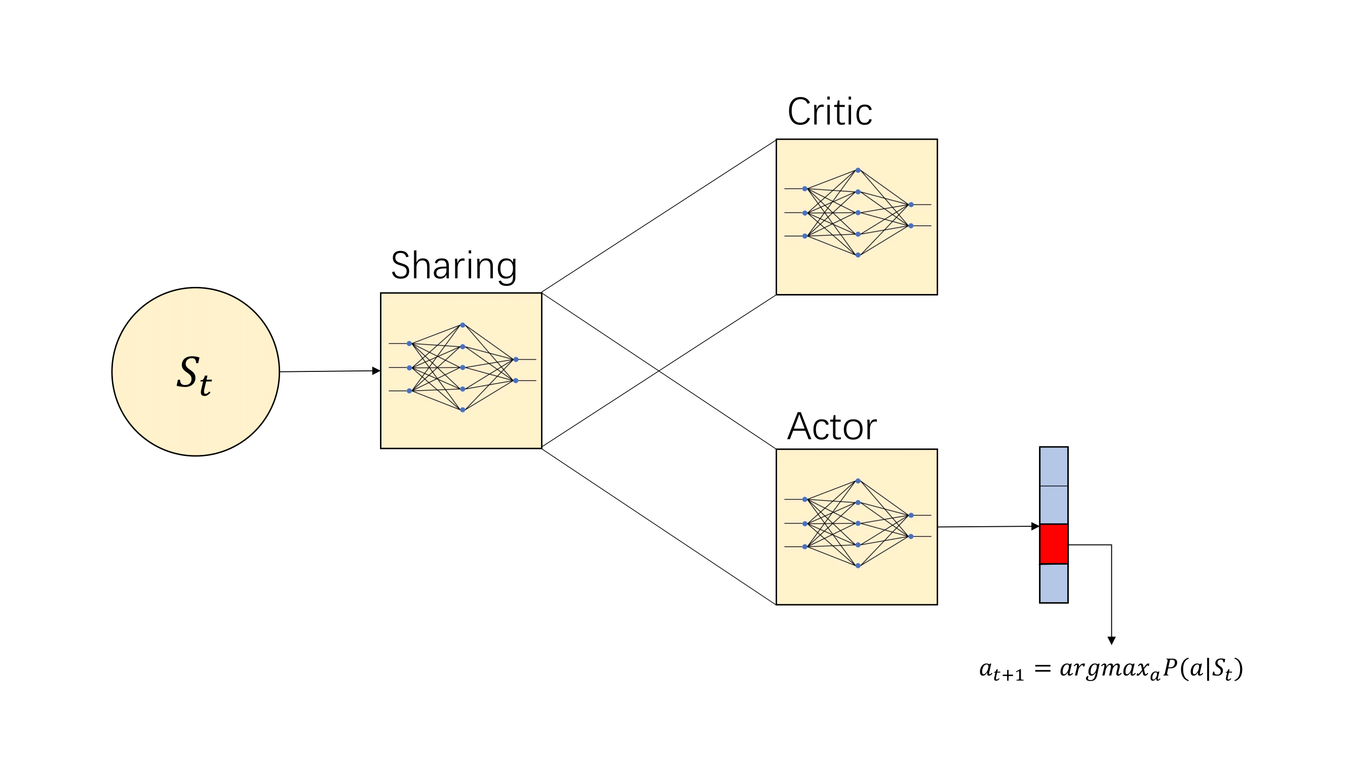
Figure 1: The partially shared neural network

IV-C Training Procedure

Algorithm 1 is the pseudo code of Advantage Actor-Critic RL Algorithm.

1 Initialized parameters $\theta$,s,$\phi$;

Initialized : Actor Network $\pi_{\theta}(s)$ and Critic Network $V^{\pi_{\theta}}_{\phi}(s)$

2 Initialized actors and critics learning rate $\gamma_{a}$ and $\gamma_{c}$ and TD error discount factor $\beta$;

3 for each training epoch $n=1,2,...,N$ do

4       Receive initial state $s_{1}$;

5       for each episode $t=1,2,...,T$ do

6             Select and Execute $a_{t}$ based on current state and policy;

7             Received $r_{t}$ and next state $s_{t+1}$ based on $(a_{t},s_{t})$;

8             Calculate TD error in critic $\delta^{\pi_{\theta}}=r+\gamma V^{\pi_{\theta}}_{\phi}\left(s_{t+1}\right)-V^{\pi_{\theta}}_{\phi}\left(s_{t}\right)$;

9             Update $\Delta\phi$ for the critic network;

10             $\Delta\phi$=$\Delta\phi$+$\delta^{\pi_{\theta}}$;

11             Calculate policy gradient in actor:

12             $\nabla_{\theta}J(\theta)=E_{\bm{\pi_{\theta}}}\left[\nabla_{\theta}\bm{\pi}_{\theta}\left(s_{t}\right)\delta^{\pi_{\theta}}\right]-\nabla_{\theta}H(\bm{\pi}_{\theta}(s_{t}))$;

13             Update $\Delta\theta$ for the policy network $\Delta\theta=\Delta\theta+\nabla_{\theta}J(\theta)$;

14             Update state: $s_{t}=s_{t+1}$;

15            

16       end for

17      Update critic network by $\Delta\phi$;

18       $\phi=\phi+\alpha\Delta\phi$;

19       Update value network by $\Delta\theta$;

20       $\theta=\theta+\beta\Delta\theta$

21 end for

22 return;

Algorithm 1 Advantage Actor-Critic RL Algorithm

V Improving by Monte Carlo Tree Search

V-A Motivation

Even if the A2C converges, it fails to detect some minor distinctions between features and tends to incorporate irrelevant features. Besides, the performance is unstable. This problem is triggered due to the model-free nature of the advantage actor algorithm. Without planning and the prior knowledge of the environment, the agent is likely to gather some noisy samples, which may lead to overfitting. Particularly, the agent seems to select irrelevant features for some samples although it performs well on others.

To further fine screen the features, we employ the Monte Carlo Tree Search (MCTS) to improve the policy learned by A2C. MCTS is a model-based algorithm for decision-making problems notably applied in games such as AlphaGo. In our task, an experiment made on the Wine dataset shows that the MCTS could reduce the cost by 0.16 on training dataset compared with the policy network learned by A2C, while maintaining the same accuracy. Thus, MCTS estimates the potential reward of introducing a feature by interaction with the environment and then uses it to adjust the policy in the best first nature, allowing us to focus on the most economic feature set.

Another advantage brought by MCTS is that it illustrates the decision rule in a tree-structure model, by which an explainable decision system can be built. In areas like healthcare and psychology, explainability is an essential prerequisite of using a model or a system. An overall diagram of the learning algorithm is plotted in Figure 2.

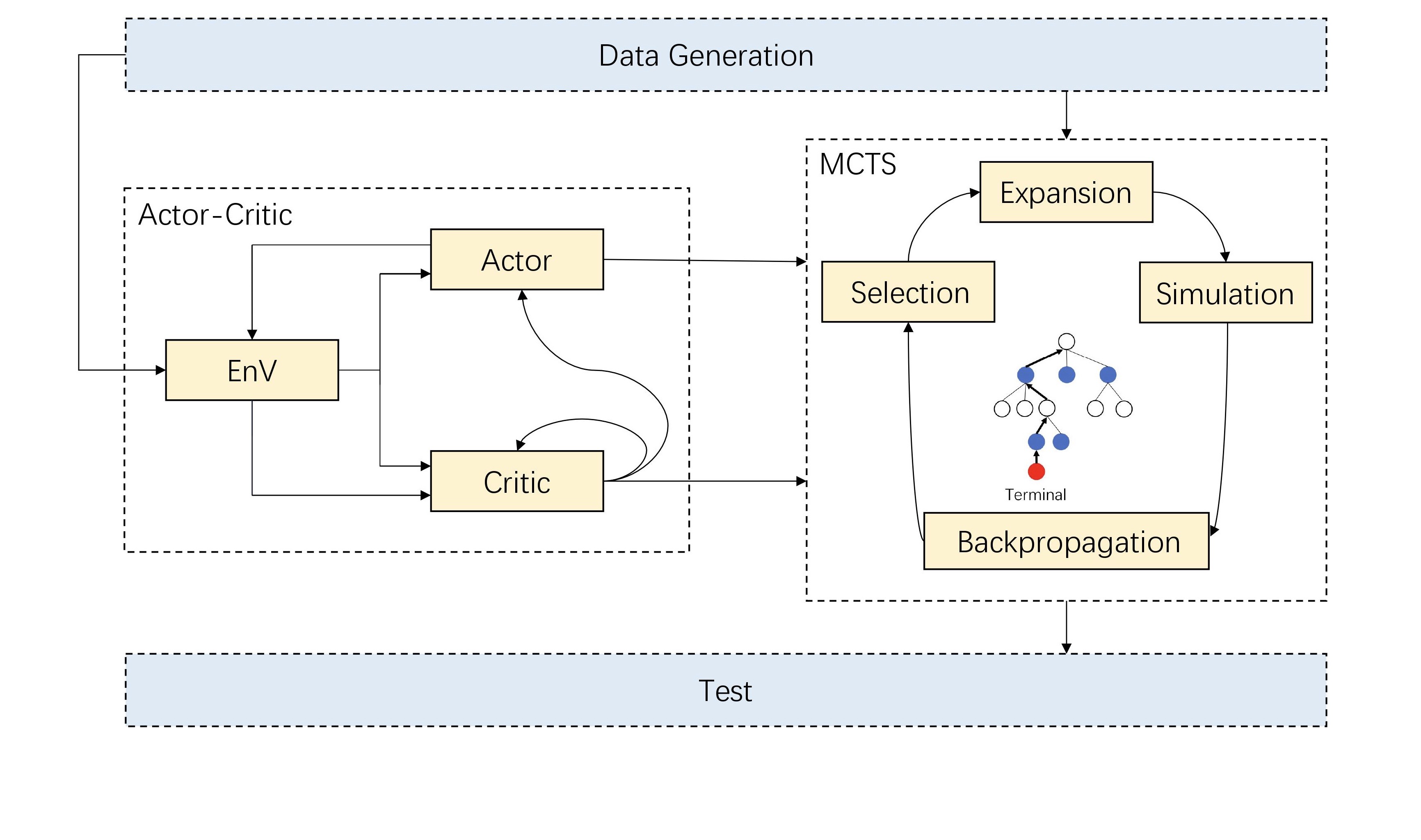
Figure 2: The system diagram of RL and MCTS

V-B Neural Monte Carlo Tree Training Procedure

In this section, we show how the Neural Monte Carlo Tree algorithm can be adapted and applied to a cost features classification. The core idea is to iteratively train the neural network $f_{\theta}$. The high-level training algorithm is shown in Algorithm 2.

Similar to the AlphaGo Zero algorithm, the MCTS here is applied as a policy improvement operator to iteratively improve the policy network[20] in the training phase. We initialize $f_{\theta}$ with the default neural network obtained from A2C to map the representation of the state $s_{t}$ to next action probability and a value, $(\textbf{p},v(s)=f_{\theta}(s))$. The vector p represents the probability of features and terminal actions to be incorporated at state $s_{t}$. Here, $v(s_{t})$ denotes the potential reward of each action. For each sample $(\textbf{x},y)$ randomly selected from training data, MCTS is adopted to search for a better policy $\bm{\pi}^{M}$ and the corresponding value estimation. These improved policies as well as the values are used as labels to train the neural network, which aims to improve the estimates of the state-value and policy functions, which, in turn, are used for MCTS in the subsequent episodes until it converges.

Specifically, for a given sample $(\textbf{x},y)$, we construct a MCTS according to the step given in Algorithm 2. Each node in the search tree contains two quantities $(Q(s_{t},a),N(s_{t},a))$: the action value function $Q(s_{t},a)$ and visiting count $N(s_{t},a)$. Here $Q(s_{t},a)$ denotes the expected long-term reward of selecting feature $a$ and $N(s_{t},a)$ denotes the number of times feature a is selected at state $s_{t}$ during the simulation. One thing needs to be mentioned is that the neural network produces $v(s_{t})$, but the MCTS requires $Q(s_{t},a)$. Hence, we use the following method to approximate it.

$$Q(s_{t},a)\approx R(s_{t},a)+\gamma V(s_{t+1})$$ (4)

When the algorithm terminates, we can calculate and collect the value and policy labels for each state to train the neural network. The reward label is already calculated before. For the policy label, we use the empirical frequency of MCTS: $\bm{\pi^{M}}(s)=\frac{N(s,.)}{\sum_{a}N(s,a)}$ to estimate it.

After gathering the improved labels, we train the neural network $f_{\theta}$ to update the policy by minimizing the loss function:

$$l=(r+v(s_{t+1})-v(s_{t}))^{2}-\bm{\pi^{M}}\mbox{log}(\bm{p})$$ (5)

where a) the first term measures the mean-square-error MSE of the predictive value function, b) the second term is the KL divergence (Kullback–Leibler divergence) between the previous policy and the policy improved by MCTS.

1:  Initialize: Initializing the neural network in MCTS with the default neural network from A2C. Set the root state as $r$, where the $\mathcal{A}_{0}$ is empty and $C_{0}$ equals zero. Set the temporal state $t\leftarrow r$

2:  Run $N$ number of MCTS simulations from $t$ according to PUCT to grow the tree.

3:  Select the action with the largest $N(t,a)$. After taking action $a$, the root state $t$ is transferred to a new state $t^{{}^{\prime}}$

4:  Update $t\leftarrow t^{{}^{\prime}}$.

5:  if $t$ is a terminal state then

6:     return: all states $t$ visited

7:  else

8:     $\mathcal{A}_{t+1}=\mathcal{A}_{t}\cup x_{a}$

9:     $C_{t+1}=C_{t}+c_{a}$

10:     return to step 2

11:  end if

Algorithm 2 Constructing an MCTS tree for a single $(\bm{x},y)$ pair

V-C Neural Monte Carlo Tree Search

Details of how the MCTS works in our task requires clarification. Each node in the tree is associated with 4 quantities $(s_{t},Q(s_{t},a),\pi(s_{t},a),N(s_{t},a))$. As illustrated in Figure 3, at each iteration, MCTS performs four steps: selection, expansion, simulation, and backpropagation. In particular, starting from the current root state $s_{t}$, we select action $a_{t}$ according to PUCT (Polynomial Upper Confidence bound for Trees):

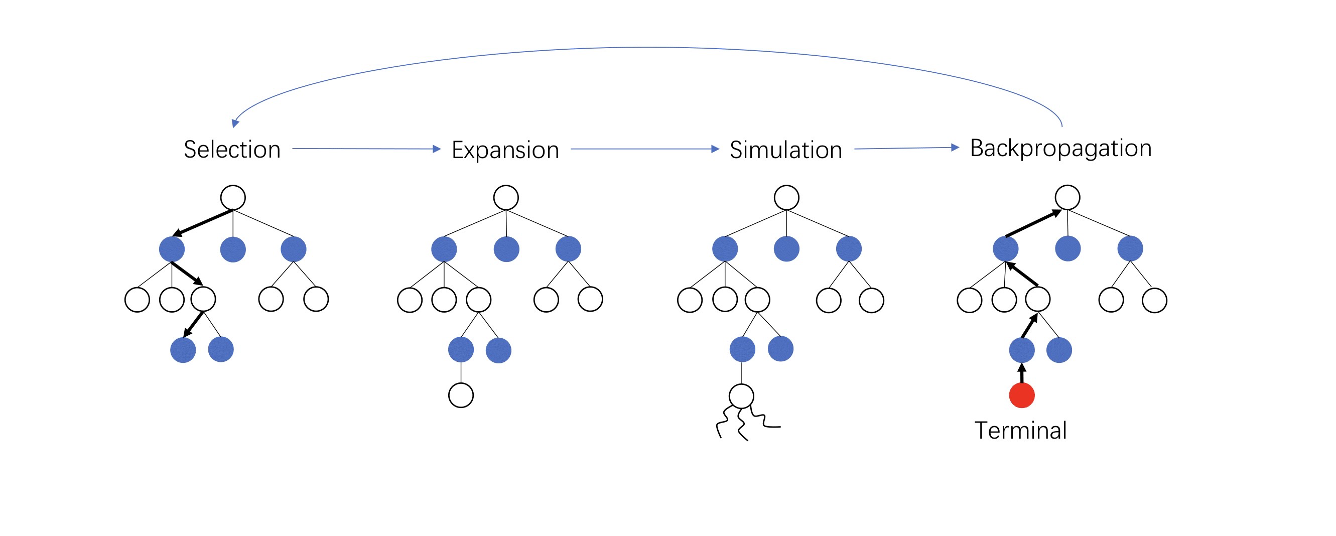
Figure 3: The growth of MCTS

$$a_{t}=\arg\max_{a}\left\{Q(s_{t},a)+c\cdot\pi_{\theta}(s_{t},a)\frac{\sqrt{\sum_{b}N(s_{t},b)}}{N(s_{t},a)+1}\right\},$$

Where $c$ denotes a temperature parameter balancing the exploitation and exploration. Instead of totally relying on the roll-out step, using a neural network to guide the search reduces both the breadth and depth of the space, leading to a significant speedup. Once the agent selects a terminal action or the size of the feature subset exceeds a constant $T$, we stop searching and propagate the obtained reward along the search path back to the root for all the states visited previously. In our experiment, $T$ is set to be 80 percent of the total number of features. The $Q$ value and the value of $N$ will be updated according to the formula:

$$N(s_{t},a_{t})\leftarrow N(s_{t},a_{t})+1$$ (6)

$$Q(s_{t},a_{t})\leftarrow\frac{(N(s_{t},a_{t})-1)Q(s_{t},a_{t})+v(s_{t})}{N(s_{t},a_{t})}$$ (7)

TABLE I: Datasets from UCI

Dataset	Number of Features	Class	Number of observations
Wine	13	3	70
Yeast	8	10	600
Aba	7	2	4177
Bld	6	2	345
Cir	10	2	1000
Pid	7	2	532
Rng	10	2	1000

VI Experiment

We compared our A2C+MCTS methods with other costly features classification algorithms and conducted an empirical study to evaluate their performance on both balanced data and imbalanced data. Data with different levels of imbalance ratio is generated to illustrate how different levels of imbalance ratio will affect the algorithm’s performance. We also made an exploration on reward value to investigate the relation between reward and imbalance ratio.

TABLE II: ACCURACY (COST) OF A2C+MCTS ALGORITHM VS EXISTING ALGORITHMS

balance				Q
	A2C+MCTS	Adapt-Gbrt	BudgetPrune	RADIN	DWSM	DQN	DNN (Full Data)	RF (Full Data)
Wine	$\mathbf{0.82\ (5.5)}$	NA	$0.7\ (4.1)$	$0.8\ (3.9)$	$0.77\ (5.5)$	$0.8\ (5.2)$	$0.89\ (10.7)$	$0.91\ (10.7)$
Yeast	$\mathbf{0.51\ (2.8)}$	NA	$0.47\ (3.2)$	$0.43\ (2.3)$	$0.46\ (3)$	$\mathbf{0.51\ (2.5)}$	$0.55\ (6.8)$	$0.58\ (6.8)$
Ada	$\mathbf{0.73\ (3.2)}$	$0.66\ (1.9)$	$0.61\ (3.2)$	$0.58\ (3.7)$	$0.65\ (2.4)$	$0.71\ (3.1)$	$0.75\ (5.9)$	$0.78\ (5.9)$
Bld	$\mathbf{0.61\ (3)}$	$0.47\ (2.3)$	$0.49\ (2.6)$	$0.42\ (1.8)$	$0.53\ (2.1)$	$0.59\ (2.7)$	$0.72\ (5.6)$	$0.71\ (5.6)$
Cir	$\mathbf{0.65\ (6.1)}$	$0.49\ (6.3)$	$0.51\ (5.2)$	$0.43\ (5.3)$	$0.56\ (5.9)$	$0.63\ (6.2)$	$0.76\ (9.1)$	$0.78\ (9.1)$
Pid	$\mathbf{0.79\ (3.4)}$	$0.53\ (3.9)$	$0.71\ (4.2)$	$0.67\ (2.9)$	$0.69\ (3.4)$	$0.77\ (3.6)$	$0.78\ (5.3)$	$0.77\ (5.3)$

VI-A Comparison methods

Several costly features classification algorithms are proposed and compared to our methods, Some are post-hoc algorithms, building the model based on a well trained algorithm. Others are designed without considering other frameworks. Besides, we use Deep Neural Network Network(DNN) and Random Forests(RF) as two basic models as the baseline model. These two methods are trained by using all features.

Adapt-Gbrt: A random forest based model and it trains a high-accuracy complex(HPC) model. With HPC, it jointly learns a gating function and prediction on fully labeled training data by means of a bottom-up strategy. However, it could only deal with binary class datasets. Thus, we won’t show its performance on multi-class datasets.

BudgetPrune: A post-hoc pruning model. Based on the well trained random forest classifier, it prunes the RF by linear programming to balance between cost and accuracy[21].

RADIN: An adaptive learning method by using recurrent neural networks(RNN) with attention to select a fixed block of features and also fix the selection step[22].

DWSM:A method to formalize the task as an Markov decision process(MDP) and solve it with linearly approximated Q-learning[13].

DQN: A method similar to DWSM. It replaces the linear approximation function by a deep neural network and using a pretarined HPC[14].

ROS: A method to build a more balanced dataset by over-sampling the minority samples[23].

CSM: A cost sensitive method by punishing harshly on the misclassification of minority samples[24].

VI-B Evaluation metrics

In order to make a fair and comprehensive comparison, we use accuracy as the measure for the balance data, and G-mean score for the imbalance data. G-mean score is the geometric mean of recall and specificity. The better algorithm tends to produce a higher G-mean score on imbalance data. The formulae of G-mean are shown as follows:

$$\mbox{G-mean}=\sqrt{\mbox{Recall}*\mbox{Specificity}}$$

Where $\mbox{Recall}=\frac{\mbox{TP}}{\mbox{TP}+\mbox{FN}}$, and $\mbox{Specificity}=\frac{\mbox{TN}}{\mbox{TN}+\mbox{FP}}$. TP describes the number of positive data, TN denotes the number of true negative data, FP illustrates the number of false positive data and FN is the number of false negative data.

VI-C Dataset and Network Architecture

To validate the performance of our model, we use several datasets from UCI as shown in TableI. All of them are multi-class datasets with a number of features ranging from 6-50 and classes ranging from 2-10. All the datasets are assigned random costs from 0.1 to 1 according to the previous experiment. The details of the data set could be found in Table2. For each experiment, we normalize the datasets with their mean and standard deviation and split them into training,validation and testing sets. Note that our results are calculated by randomly splitting the datasets for 30 times. We use the partially shared deep neural network to learn the feature representation from the dataset. We use three fully connected layers for the sharing part and two fully connected layers for the policy part and value part. For our model, the network architecture is similar to the network used in AlphaGo zero.

TABLE III: G-mean SCORE (COST) ON IMBALANCED DATA

	Imbalanced Ratio	A2C+MCTS	DQN	Adapt-Gbrt	ROS (Full Data)	CSM (Full Data)
	$5\%$	$0.73\ (7.3)$	$0.58\ (6.6)$	$0.42\ (3.6)$	$0.71\ (9.1)$	$0.75\ (9.1)$
Cir	$10\%$	$0.79\ (6.7)$	$0.63\ (5.7)$	$0.51\ (3.7)$	$0.76\ (9.1)$	$0.80\ (9.1)$
	$20\%$	$0.83\ (6.7)$	$0.75\ (5.6)$	$0.52\ (3.9)$	$0.79\ (9.1)$	$0.83\ (9.1)$
	$5\%$	$0.83\ (6.9)$	$0.79\ (6.5)$	$0.69\ (4.3)$	$0.82\ (9.3)$	$0.85\ (9.3)$
Rng	$10\%$	$0.86\ (5.8)$	$0.82\ (6.3)$	$0.71\ (4.5)$	$0.85\ (9.3)$	$0.87\ (9.3)$
	$20\%$	$0.87\ (5.8)$	$0.83\ (6.2)$	$0.76\ (4.1)$	$0.87\ (9.3)$	$0.88\ (9.3)$

VI-D Experiment results

VI-D1 Balanced Data

Before the experiment of imbalanced data, we compare our A2C model with other algorithms on balanced data sets. We assign the reward $\delta$ to be 1. For fairness and convincing comparison, we tune other methods for their best performance. The results are shown in Table II. We can clearly see that our A2C+MCTS method achieves an outstanding performance with a moderate cost compared to DQN and Adapt-Gbrt. In each experiment, our method has a similar cost budget as DQN, but has a higher accuracy. BudgetPrune and RADIN, according to their intuition, are efficient algorithms which tend to select features with a small cost. Their performance, however, is not comparable to other methods. Although using a small subset of features[25][26][27], we can clearly observe that A2C+MCTS and DQN can get similar accuracy compared to DNN and RF, with an economically selected subset of features.

VI-D2 Imbalanced Data

We report the G-mean score on the datasets Cir and Rng. We construct the new dataset according to the imbalance ratio $\rho$. Similar to the balanced data, we compared A2C+MCTS to other algorithms and showed the result in Table III. As shown in Table III, with the increase of data imbalance level, the G-mean scores of each method suffer a serious reduction. It is clear that neither DQN nor Adapt-Gbrt can deal with the imbalanced data. Specifically, Adapt-Gbrt, although has a smaller cost than A2C+MCTS and DQN, performs worse as the imbalance ratio decreases due to its post-hoc nature. Meanwhile, we also adopt two imbalanced data classification algorithms: CSM and ROS, as two baselines on the complete dataset. We can observe that A2C+MCTS can beat ROS by using a subset of features.

VI-E Ablation Study

VI-E1 MCTS

Here we show the importance of using MCTS embedded with the Actor Critic pretrained model. The comparison is shown in Table IV Before using the MCTS, actor critic can only achieve a sub-optimal result due to its lack of prior knowledge about the environment. Besides, actor critic tends to incorporate more irrelevant features compared to the A2C+MCTS algorithm.

VI-E2 A2C

This experiment is implemented by 2 CPU. We test the MCTS searching time on one sample and draw the histogram in Figure 4. This histogram reveals that MCTS is orders of magnitude faster with the A2C pretrained model. This could be contributed to the value estimation function of actor critic neural network, which serves as a special pruning algorithm when embedded into the neural monte carlo tree.

TABLE IV: IMPORTANCE OF MCTS

	A2C	A2C+MCTS
Cir	$0.57\ (8.5)$	$0.65\ (6.1)$
Pid	$0.63\ (4.2)$	$0.79\ (3.4)$
Bld	$0.55\ (3.9)$	$0.61\ (3.0)$

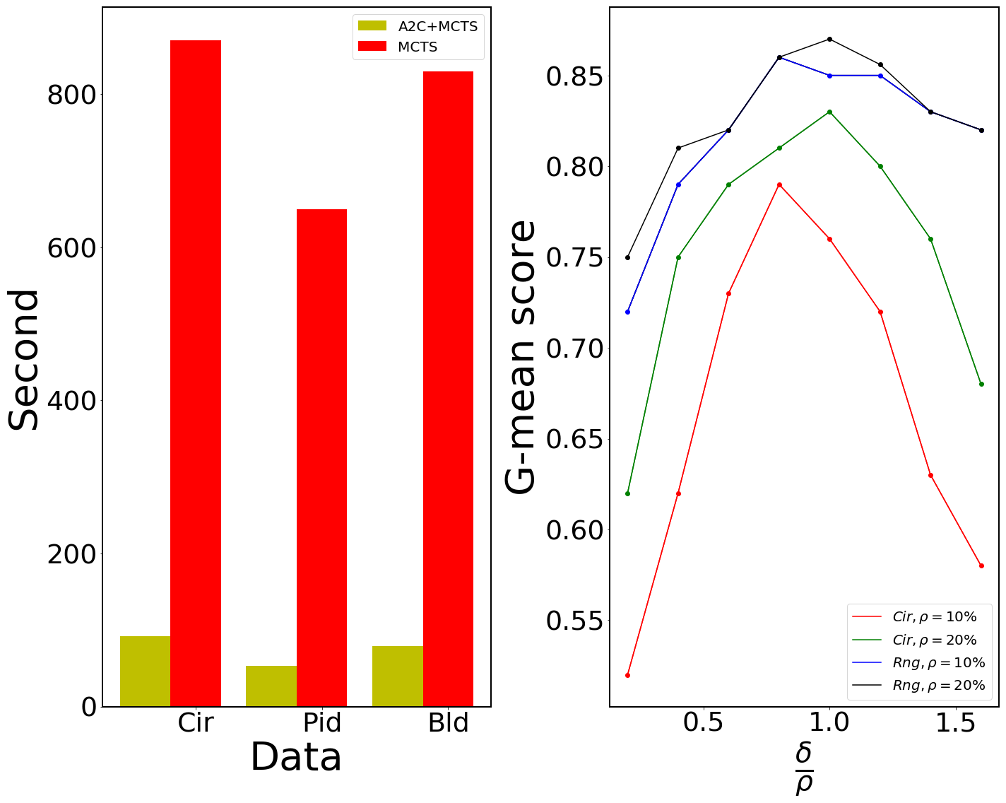
Figure 4: LEFT:Searching time for MCTS in one episode. Right: G-mean Score with different reward value on imbalanced dataset

VI-E3 Reward Exploration

Reward function is used to encourage the agent to select important and economic features before making predictions. In an experiment on a balanced dataset, we set the reward as 1. In another imbalanced dataset, we treat the reward for the majority sample $\delta$ as a parameter and tune it. To study the effect of different $\delta$ on the classification performance, we try different value of $\delta$ on multiple dataset and show their G-mean score on Figure 4 (Right), where $\delta\in\{0.2\rho,0.4\rho,0.6\rho,0.8\rho,\rho,1.2\rho,1.4\rho,1.6\rho\}$.

In both datasets, we can clearly see that the largest G-mean score is achieved when the $\delta$ is close to $\rho$. When $\delta=\rho$, the majority and minority samples exert the same impact on the gradient of the actor critic network. When $\delta>\rho$, the majority samples have more influence and the performance is declined. Thus, it makes sense to set $\delta<\rho$. Note that the optimal $\delta$ is a little smaller than $\rho$ as shown in the plot, which suggests we slightly increase the influence of minority samples over majority samples.

VII Conclusion

We propose an A2C+MCTS two stage algorithm for the cost features classification problem. Different from other algorithms, we leverage the actor critic framework to improve the stability of the model. To be efficient, we use the MCTS to further improve the policy learnt by A2C. Besides, we also consider the explainability of the model. Further research could be left to explore more efficient algorithms to extract the decision rule from the monte carlo tree.

References

- [1] J. Liu, H. Shen, H. Chi, H. S. Narman, Y. Yang, L. Cheng, and W. Chung, “A low-cost multi-failure resilient replication scheme for high-data availability in cloud storage,” IEEE/ACM Transactions on Networking, 2020.
- [2] Y. Wu, W. AdbAlmageed, S. Rawls, and P. Natarajan, “Computationally efficient template-based face recognition,” in 2016 23rd International Conference on Pattern Recognition (ICPR), pp. 1424–1429, IEEE, 2016.
- [3] B. Jin, L. Cruz, and N. Goncalves, “Deep facial diagnosis: Deep transfer learning from face recognition to facial diagnosis,” IEEE Access, vol. 8, pp. 123649–123661, 2020.
- [4] O. Y. Al-Jarrah, P. D. Yoo, S. Muhaidat, G. K. Karagiannidis, and K. Taha, “Efficient machine learning for big data: A review,” Big Data Research, vol. 2, no. 3, pp. 87–93, 2015.
- [5] D. N. Vinod and S. Prabaharan, “Data science and the role of artificial intelligence in achieving the fast diagnosis of covid-19,” Chaos, Solitons & Fractals, vol. 140, p. 110182, 2020.
- [6] S. Dang, M. Wen, S. Mumtaz, J. Li, and C. Li, “Enabling multi-carrier relay selection by sensing fusion and cascaded ann for intelligent vehicular communications,” IEEE Sensors Journal, 2020.
- [7] C. Hou, Y. Wen, Y. He, X. Liu, M. Wang, Z. Zhang, and H. Fu, “Public stereotypes of recycled water end uses with different human contact: Evidence from event-related potential (erp),” Resources, Conservation and Recycling, vol. 168, p. 105464, 2021.
- [8] S. J. Chen, A. Choi, and A. Darwiche, “Value of information based on decision robustness,” in Twenty-Ninth AAAI Conference on Artificial Intelligence, 2015.
- [9] S. J. Chen, A. Choi, and A. Darwiche, “Algorithms and applications for the same-decision probability,” Journal of Artificial Intelligence Research, vol. 49, pp. 601–633, 2014.
- [10] L.-P. Liu, Y. Yu, Y. Jiang, and Z.-H. Zhou, “Tefe: A time-efficient approach to feature extraction,” in 2008 Eighth IEEE International Conference on Data Mining, pp. 423–432, IEEE, 2008.
- [11] F. Nan and V. Saligrama, “Adaptive classification for prediction under a budget,” in Advances in neural information processing systems, pp. 4727–4737, 2017.
- [12] S. Maliah and G. Shani, “Mdp-based cost sensitive classification using decision trees,” in Thirty-Second AAAI Conference on Artificial Intelligence, 2018.
- [13] G. Dulac-Arnold, L. Denoyer, P. Preux, and P. Gallinari, “Datum-wise classification: a sequential approach to sparsity,” in Joint European Conference on Machine Learning and Knowledge Discovery in Databases, pp. 375–390, Springer, 2011.
- [14] J. Janisch, T. Pevnỳ, and V. Lisỳ, “Classification with costly features using deep reinforcement learning,” in Proceedings of the AAAI Conference on Artificial Intelligence, vol. 33, pp. 3959–3966, 2019.
- [15] C. B. Browne, E. Powley, D. Whitehouse, S. M. Lucas, P. I. Cowling, P. Rohlfshagen, S. Tavener, D. Perez, S. Samothrakis, and S. Colton, “A survey of monte carlo tree search methods,” IEEE Transactions on Computational Intelligence and AI in games, vol. 4, no. 1, pp. 1–43, 2012.
- [16] M. Babaeizadeh, I. Frosio, S. Tyree, J. Clemons, and J. Kautz, “Reinforcement learning through asynchronous advantage actor-critic on a gpu,” arXiv preprint arXiv:1611.06256, 2016.
- [17] Z. Chen, J. Hu, and G. Min, “Learning-based resource allocation in cloud data center using advantage actor-critic,” in ICC 2019-2019 IEEE International Conference on Communications (ICC), pp. 1–6, IEEE, 2019.
- [18] W. Cai and Z. Wei, “Remote sensing image classification based on a cross-attention mechanism and graph convolution,” IEEE Geoscience and Remote Sensing Letters, 2020.
- [19] D. Silver, J. Schrittwieser, K. Simonyan, I. Antonoglou, A. Huang, A. Guez, T. Hubert, L. Baker, M. Lai, A. Bolton, et al., “Mastering the game of go without human knowledge,” nature, vol. 550, no. 7676, pp. 354–359, 2017.
- [20] J. Huang, M. Patwary, and G. Diamos, “Coloring big graphs with alphagozero,” arXiv preprint arXiv:1902.10162, 2019.
- [21] F. Nan, J. Wang, and V. Saligrama, “Pruning random forests for prediction on a budget,” arXiv preprint arXiv:1606.05060, 2016.
- [22] G. Contardo, L. Denoyer, and T. Artières, “Recurrent neural networks for adaptive feature acquisition,” in International Conference on Neural Information Processing, pp. 591–599, Springer, 2016.
- [23] C. Drummond, R. C. Holte, et al., “C4. 5, class imbalance, and cost sensitivity: why under-sampling beats over-sampling,” in Workshop on learning from imbalanced datasets II, vol. 11, pp. 1–8, Citeseer, 2003.
- [24] Z.-H. Zhou and X.-Y. Liu, “Training cost-sensitive neural networks with methods addressing the class imbalance problem,” IEEE Transactions on knowledge and data engineering, vol. 18, no. 1, pp. 63–77, 2005.
- [25] H. Liu, C. Liu, and Y. Huang, “Adaptive feature extraction using sparse coding for machinery fault diagnosis,” Mechanical Systems and Signal Processing, vol. 25, no. 2, pp. 558–574, 2011.
- [26] Y. Q. Chen, O. Fink, and G. Sansavini, “Combined fault location and classification for power transmission lines fault diagnosis with integrated feature extraction,” IEEE Transactions on Industrial Electronics, vol. 65, no. 1, pp. 561–569, 2017.
- [27] Y. Fan, Q. Wen, W. Wang, P. Wang, L. Li, and P. Zhang, “Quantifying disaster physical damage using remote sensing data—a technical work flow and case study of the 2014 ludian earthquake in china,” International Journal of Disaster Risk Science, vol. 8, no. 4, pp. 471–488, 2017.