Abstract

Structured matrices, such as those derived from Kronecker products (KP), are effective at compressing neural networks, but can lead to unacceptable accuracy loss when applied to large models. In this paper, we propose the notion of doping - addition of an extremely sparse matrix to a structured matrix. Doping facilitates additional degrees of freedom for a small number of parameters, allowing them to independently diverge from the fixed structure. To train LSTMs with doped structured matrices, we introduce the additional parameter matrix while slowly annealing its sparsity level. However, we find that performance degrades as we slowly sparsify the doping matrix, due to co-matrix adaptation (CMA) between the structured and the sparse matrices. We address this over dependence on the sparse matrix using a co-matrix dropout regularization (CMR) scheme. We provide empirical evidence to show that doping, CMA and CMR are concepts generally applicable to multiple structured matrices (Kronecker Product, LMF, Hybrid Matrix Decomposition). Additionally, results with doped kronecker product matrices demonstrate state-of-the-art accuracy at large compression factors ($10-25\times$) across 4 natural language processing applications with minor loss in accuracy. Doped KP compression technique outperforms previous state-of-the art compression results by achieving $1.3-2.4\times$ higher compression factor at a similar accuracy, while also beating strong alternatives like pruning and low-rank methods by a large margin (8% or more). Additionally, we show that doped KP can be deployed on commodity hardware using the current software stack and achieve $2.5-5.5\times$ inference run-time speed-up over baseline.

1 Introduction

Language models (LMs) based on neural networks have been extremely effective in enabling a myriad of natural language processing (NLP) applications in recent years. However, many of these NLP applications are increasingly being deployed on consumer mobile devices and smart home appliances, where the very large memory footprint of large LMs is a severe limitation. To help bridge this gap in model size, model optimization techniques have been demonstrated to reduce the memory footprint of the weight matrices Fedorov et al. (2019); Dennis et al. (2019); Kusupati et al. (2018). However, results published to date still result in very significant off-chip DRAM bandwidth, which increases the power consumption of mobile devices Li et al. (2019). This is especially significant for NLP applications that are running for long periods of time. For example, to efficiently deploy a 25 MB LM on a device with 1 MB L2 cache, requires 25$\times$ compression or a 96% reduction in the number of parameters. Such a high pruning ratio leads to significant accuracy degradtion (Gale et al. (2019b); Zhu & Gupta (2017)), which is not acceptable from an application point of view. Therefore, to enable efficient inference on resource constrained devices Zhu et al. (2019), there is a sustained need for improved compression techniques that can achieve high compression factors without compromising accuracy.

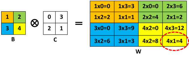
(a) Conventional Kronecker product matrix.

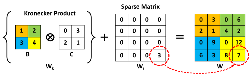
(b) Doped Kronecker product matrix.

Figure 1: In the conventional Kronecker product (a), individual elements in the expansion $W$ cannot diverge independently without impacting other elements in the block. This restricts freedom in the parameter space and limits accuracy. By doping with a sparse matrix $M_{sp}$ (b), we relax this constraint with an additional degree of freedom in the parameter space, with minimal overhead.

Model compression using structured matrices has been previously demonstrated on various image and audio tasks, such as object detection, human activity recognition (HAR), orthogonal projections and key-word spotting (KWS) Thomas et al. (2018); Sindhwani et al. (2015); Ding et al. (2017a); Deng et al. (2018); Thakker et al. (2019c). For example, Kronecker Products (KP) were used to compress HAR and KWS models by 15-38$\times$ compression factors Thakker et al. (2019a) while achieving better accuracy than other traditional compression techniques such as pruning Zhu & Gupta (2017) and low-rank matrix factorization (LMF).However, applying KP to more complex tasks, such as a large LM, results in a 26% loss in perplexity, while applying a low rank structure using tensor train decomposition leads to a greater than 50% decrease in perplexity score Grachev et al. (2019). Figure 1(a) shows that the root issue with conventional KP is that during the optimization of the constituent matrices $B$ and $C$, all elements of $W$ inside each block of 4 elements (colored in the figure) are related. This limitation in the parameter space leads to perplexity loss on larger problems. Specifically, the issue gets exaggerated in bigger matrices as structured decomposition of bigger matrices for large compression factors creates more number of such relations. Other structured matrices Thomas et al. (2018) face a similar challenge.

In this paper, we relax this limitation in the parameter space by doping the structured matrix $M_{k}$ with an extremely sparse additive matrix $M_{s}$ (Figure 1(b)). This approach was inspired by robust PCA techniques, and allows an additional degree of freedom to recover accuracy at very low inference-time cost. The contributions of this paper are further summarized below:

• We propose sparse matrix doping, which addresses the accuracy limitations of structured matrix compression using an additional sparse matrix with negligible inference cost.

• A training recipe to learn the structured and the sparse matrix, describing regularization techniques to reduce the co-matrix adaptation (CMA) encountered as we anneal sparsity, using co-matrix regularization (CMR).

• Show that doping, CMA and CMR are applicable to a a wide variety of structured matrices.

• Present state-of-the-art results for compressing language models and translation applications using doped KP, which are 1.5$\times$ - 2.4$\times$ smaller than previous work at comparable accuracy values.

The remainder of the paper is organized as follows. Section 2 briefly surveys related work. Section 3, introduces sparse matrix doping by applying the technique to Kronecker product matrix compression, which is the main focus of the paper. We discuss the challenges in training doped structured matrices (Section 4) and propose a training recipe that includes regularization to prevent co-matrix adaptation which otherwise leads to accuracy loss (Section 5). Using this training recipe, we discuss how doped structured matrix compression techniques can be applied to a variety of structured matrices in Section 6.2 and discuss why doped KP leads to higher accuracy than other structured matrices evaluated in this paper. We demonstrate state-of-the art models using doped KP compression on three language modeling tasks and one translation task in Sections 6.3.1,6.3.2 and 6.3.3. Doping introduces negligible run-time overhead, which we confirm by benchmarking the inference performance of all models on a Raspberry Pi 4 (Section 6.3.5).

2 Related Work

Random Pruning Han et al. (2016); Zhu & Gupta (2017); Sanh et al. (2020); Fedorov et al. (2020); Whatmough et al. (2018); Liu et al. (2020); Whatmough et al. (2019) of neural networks seems to be a very successful compression technique across many different tasks. However, so-called random pruning is hard to exploit on real hardware due to the lack of regularity in the resulting matrix multiplications unless the sparsity level is large.

Structured Matrices have shown significant potential for compression of neural networks Sindhwani et al. (2015); Ding et al. (2018; 2017b); Cheng et al. (2015); Zhou et al. (2015); Thomas et al. (2018); Thakker et al. (2019a; 2020b). Block circular compression is an extension of structured matrix based compression technique, converting every block in a matrix into a structured matrix. Building on top of this, our work proposes a method to increase the compression achieved using structured matrices at baseline accuracy by introducing sparse matrix doping on top of structured matrices.

Tensor Decomposition including Tucker decomposition, Kronecker etc. These methods have also been employed to achieve significant reduction in parameters Tjandra et al. (2017); Gope et al. (2019; 2020b). Low-rank Matrix Factorization (LMF) Kuchaiev & Ginsburg (2017); Chen et al. (2018); Grachev et al. (2017); Thakker et al. (2019; 2020a) can also be categorized under this topic. LMF aware NN are a special case of structured matrix as it also imposes a certain constraint on the expressibility of the matrix. We will show in this paper that doped KP can lead to better accuracy than LMF.

Quantization is another popular technique for compression Hubara et al. (2017; 2016); Sanh et al. (2019); Liu et al. (2018); Gope et al. (2020a); Banbury et al. (2021). Networks compressed using DKP can be further compressed using quantization.

Dynamic techniques are used to improve inference run-time of RNNs by skipping certain RNN state updates Campos et al. (2018); Seo et al. (2018); Yu et al. (2017); Tao et al. (2019). These techniques are based on the assumption that not all inputs to an RNN are needed for final classification task. Thus we can learn a small and fast predictor that can learn to skip certain inputs and its associated computation. Doped KP technique is orthogonal to this technique and networks compressed using doped KP can be further optimized using this technique. These dynamic techniques could be extended to networks beyond LSTMs also Raju et al. (2020); Huang et al. (2020).

Efficient Network Architectures for LSTMs, such as SRU Lei et al. (2018), QRNN Bradbury et al. (2016) and PRU Mehta et al. (2018) have also led to networks with faster inference run-time performance through increased parameter efficiency. Doped KP can be used to compress the weight matrices in all of these architectures to further optimize the inference time performance.

Word Embedding Compression is another way to reduce the parameter footprint of embedding matrices in NLP Acharya et al. (2019); Mehta et al. (2019). In this paper, we show that DKP can compress networks with compressed word embedding layers also.

Combining features: The doped KP compression technique replaces a weight matrix with the sum of a sparse additive matrix and a structured matrix. This leads to output features that are a combination of those generated from a structured matrix and another from a sparse matrix. Kusupati et al. (2018) and He et al. (2015) also combine features from two different paths. However, their work deviates from ours for multiple reasons. Firstly, their aim is to combine features to tackle the vanishing gradients issue. Secondly, they use a residual connection for the additive feature, and as a result, they do not see the CMA issue discussed in our work. Finally, their technique is not well suited for the purpose of enabling additional degrees of freedom in features constrained by a structured matrix. Specifically, the sparse matrix selects specific elements in a feature vector that need additional degrees of freedom which their work cannot do.

In this work, doped KP combines very high-sparsity random pruning with structured matrix techniques. Our results are compared with pruning, structured matrix and tensor decomposition techniques. Quantization can subsequently be used to further compress the models we present.

3 Doped Kronecker Product

In this paper we will focus on applying the doping technique to Kronecker product structured matrices. However, doping can be generalized to other structured matrices and we will also give some results for other structures in Section 6.

Let lowercase and uppercase symbols denote vectors and matrices, respectively. In doped KP, a parameter matrix $W$ is the sum of a KP matrix $W_{k}$ and a sparse matrix $W_{s}$ (Figure 1(b)),

$$W=W_{k}+W_{s},$$ (1)

$$W_{k}=B\otimes C,$$ (2)

where, $\otimes$ represents the Kronecker operator Nagy (2009) For $B\in\mathbb{R}^{M1\times N1}$, $C\in\mathbb{R}^{M2\times N2}$, $W\in\mathbb{R}^{M\times N}$, $M=M1\times M2$ and $N=N1\times N2$ the compression factor (CF) can be calculated using the formula:

$$CF=(M1*N1+M2*N2+\left\lVert W_{s}\right\lVert_{0})/(M*N).$$ (3)

3.1 Sizing doped KP Matrices

Identifying the dimensions of the $B$ and $C$ matrices is non-trivial. A matrix can be expressed as a KP of multiple smaller matrices of varying sizes. For example, if $\boldsymbol{W_{k}}$ is of size 100$\times$100, B and C can be of size $2\times 50$ and $50\times 2$ each or $10\times 10$ and $10\times 10$ each. Both solutions lead to a compression factor of $50\times$. Recent work Thakker et al. (2019a) described a straightforward methodology to achieve maximum compression of $W_{k}$ using KP, while achieving maximum rank. Empirical evidence suggests that the large rank value corresponds to larger accuracy gains. Therefore, we adopt the methodology in Thakker et al. (2019a) to decompose $W_{k}$ into $B$ and $C$. We run ablation studies to further confirm that this choice indeed holds true. The results of these ablation studies can be found in Appendix A.

Once the size of $W_{k}$ is fixed, $\left\lVert W_{s}\right\lVert_{0}$ can be set during hyperparameter optimization, to maximize the compression factor without impinging on performance. As an example, if $\boldsymbol{W}$ is of size 100$\times$100, $\boldsymbol{B}$ and $\boldsymbol{C}$ are of size 10$\times$10, then 95% sparsity in $\boldsymbol{W}_{s}$ results in a compression factor of 14$\times$; the same scenario with 90% sparsity in $\boldsymbol{W_{s}}$ results in an 8.4$\times$ compression factor.

3.2 Training doped KP Networks

The doped KP networks are trained from scratch, i.e. they do not start from a pre-trained network. Doped KP replaces all the parameter matrices in the neural network with the sum of $W_{k}$ and $W_{s}$ matrices. We initially set $W_{s}$ with a dense random initialization. Then, as training progresses, we apply magnitude weight pruning to $W_{s}$, annealing the sparsity towards the target level. We use the methodology described in Zhu & Gupta (2017) to achieve this transition, which aims to allow the training optimization algorithm to retain the non-zero elements in $W_{s}$, which have the greatest impact on cross entropy.

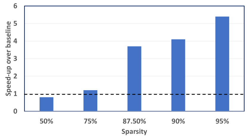
Figure 2: Speed-up of matrix-vector product kernels as a function of matrix sparsity, with a dense vector. The matrix is of dimension $256\times 256$. Measured on a single Arm Cortex A-72 CPU of the Raspberry Pi 4 board using the Eigenc C++ library.

3.3 Inference on doped KP Networks

For inference on an edge device, NLP applications generally use a batch size of one and thus execute a matrix-vector product kernel Thakker et al. (2019b). The matrix vector product for doped KP will lead to the execution of the following computation:

$$y =W*x$$ (4)

$$y =(W_{k}+W_{s})*x,\;where$$ (5)

$$W_{k} =B\otimes C,$$ (6)

where,$W\in R^{M\times N}$, $x\in R^{N\times 1}$, $y\in R^{M\times 1}$, $B\in R^{M1\times N1}$, $C\in R^{M2\times N2}$, $M1\times M2=M$ and $N1\times N2=N$.

The above inference leads to multiply accumulate (MAC) and actual runtime reductions as both $W_{k}*x$ and $W_{s}*x$ can be computed cheaply.

Inference Cost of ($W_{k}*x)$:

Thakker et al. (2019a) show that to execute $W_{k}*x$ on an embedded hardware, we do not need to expand the Kronecker matrix to the larger matrix. We can achieve significant speedup by using the following set of equations Nagy (2009) -

$$y_{k} =(B\otimes C)*x$$ (7)

$$y_{k} =vec(Y_{k})\;where,$$ (8)

$$Y_{k} =C\times B\times X^{T}\;and\;X\;=\;matrix(x)$$ (9)

where $X\in R^{N2\times N1}$, $Y_{k}\in R^{M2\times M1}$, $vec()$ converts a matrix into a vector and $matrix()$ converts a vector into matrix. Thus, the matrix vector product, when the matrix is expressed as KP of two smaller matrices, gets converted into two small GEMM kernel calls.

Inference Cost of ($W_{s}*x)$:

We emphasize that the additional latency cost of doping by adding $W_{s}*x$ is negligible at inference time as long as $W_{s}$ is sufficiently sparse. Figure 2 shows the results of running matrix-vector product calculation on a Raspberry Pi 4 development board Foundation (2009), for various sparsity values of the matrix. The matrix is of dimension $256\times 256$ and the kernels use Eigen C++ library Guennebau & Jacob (2009). Clearly, the matrix sparsity has to be rather high to achieve a speedup compared to the dense baseline. However, with doping, the additional sparse matrix can be very high and therefore the additional cost is low. For example, in this paper we target $W_{s}$ sparsity values of $10\times$ or more, as a result the matrix-vector product kernel can be executed at a speed-up of $4.1\times$ or more when compared against the baseline implementation.

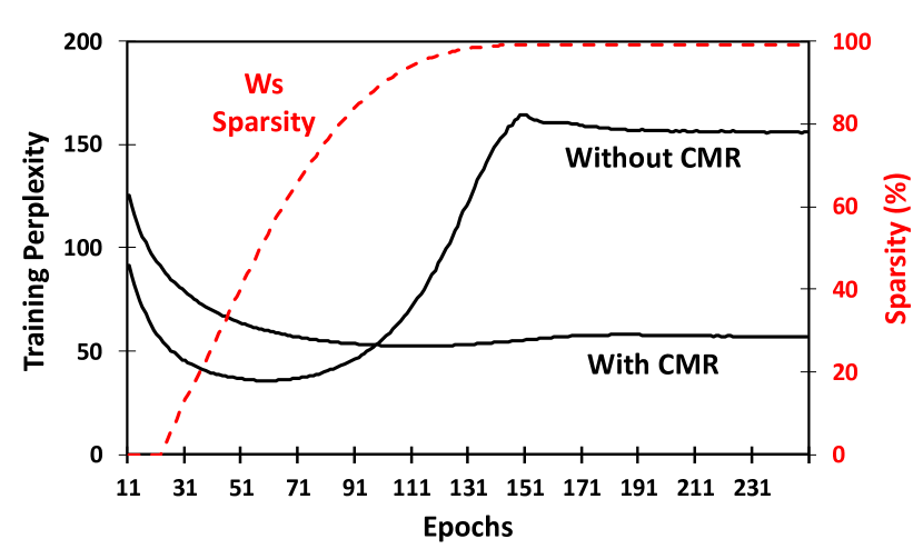
Figure 3: Training a medium LM at 100$\times$ compression. As the sparsity of $W_{s}$ is increased, training perplexity degrades due to over dependence on non-zero elements of $W_{s}$ established early on. Using CMR we are able to prevent perplexity collapse as we anneal sparsity.

4 Co-Matrix Adaptation (CMA)

Initial attempts to train doped KP LSTMs were hampered by accuracy collapse as $W_{s}$ sparsity was increased. For example, we compressed the medium LM from Zaremba et al. (2014) using KP Thakker et al. (2019a) and doped KP (Rows 2 and 3 in Table 1). However, the resulting perplexity score degrades by 44.7% when trained using doped KP, even with slightly more parameters. To clarify the source of this accuracy loss, Figure 3 shows the training perplexity and sparsity for the medium LM at an aggressive 100$\times$ CF to clearly illustrate the issue. As the sparsity of $W_{s}$ increases, the perplexity soon collapses, indicating that the model develops an over reliance on $W_{s}$ while it is dense, during the initial training phase. Subsequently, as we anneal the sparsity of $W_{s}$, the perplexity collapses. We refer to this phenomena as co-matrix adaptation (CMA).

4.1 Understanding CMA

An input feature vector $x$ in a dense layer is multiplied with the doped KP weight matrix (eq 1) to give the output $y$,

$$y=W_{k}x+W_{s}x.$$ (10)

Thus, the input flows through both $W_{k}$ and $W_{s}$ and the output of the matrix-vector product is combined to create the final output. The above equation can be viewed as,

$$y^{j}=(w_{k}^{j})^{T}x+(w_{s}^{j})^{T}x,$$ (11)

where the superscript refers to the $j^{th}$ row of the matrix. Each element of the output feature vector is the sum of neurons coming from the $W_{k}$ matrix and the $W_{s}$ matrix. CMA arises early on due to the co-adaptation of the incoming neurons through both $W_{k}$ and $W_{s}$, essentially balancing the significance of the each. However, this is problematic as we start to progressively prune $W_{s}$ as training progresses.

This co-adaptation is also obvious when we focus on the number of back-propagation updates during the initial phase of training. The rate of back-prop updates is not even between $W_{k}$ and $W_{s}$, which introduces further undesirable emphasis on the dense $W_{s}$. In the example medium LM, $B$ is 52$\times$65, and $C$ is 50$\times$20, and therefore $W_{k}$ has a total of $\sim$4.4K parameters. While $W_{s}$ is 2600$\times$1300, which is $\sim$3.4M parameters in the initial dense form. Thus, during the initial training phase, $W_{s}$ receives 700$\times$ more weight updates than $W_{k}$ leading to the over-reliance.

Compression Factor	Training Method	Sparsity of $M_{sp}$	Test Ppl.
1x	-	-	82.1
$338\times$ (KP)	-	0	104.1
$100\times$ (doped KP)	Eq 1	99%	150.7
	Eq 17a+BCD	99%	100.5
	Eq 17b+BCD	99%	100.9
	CMR	99%	95.4

Table 1: Medium LM 100$\times$ compression results using KP and DKP. Four different DKP networks are evaluated: one trained without CMR (eq 1), others trained using eq 17a, eq 17a with block coordinate descent (BCD) and CMR (eq 12). While other techniques show promising results, CMR achieves drastically improved perplexity showing that it is a more effective training technique for doped KP networks.

5 Co-Matrix Regularization (CMR)

In order to prevent undesirable reliance on non-zero elements of $W_{s}$ that will later be pruned away, we introduce a random row dropout process which we refer to as co-matrix regularization (CMR). Thus, eq 11 becomes

$$y^{j}=((\textit{w}_{k}^{j})^{T}\textit{x})\circ b_{1}+((\textit{w}_{s}^{j})^{T}\textit{x})\circ b_{2},$$ (12)

where $b_{1}$ and $b_{2}$ are CMR dropout values drawn from Bernoulli distribution with probability $p$, and $\circ$ is element-wise multiplication. CMR creates 4 different scenarios for the output neuron:

$$\;y^{j}=(\textit{w}_{k}^{j})^{T}\textit{x}+(\textit{w}_{s}^{j})^{T}\textit{x}$$ (13)

$$\;y^{j}=(\textit{w}_{k}^{j})^{T}\textit{x}$$ (14)

$$\;y^{j}=(\textit{w}_{s}^{j})^{T}\textit{x}$$ (15)

$$\;y^{j}=0\;(regular\;dropout)$$ (16)

By ensuring that the output neuron is occasionally produced without the presence of one of the incoming neurons, CMR can reduce the co-dependence between the matrices. Figure 3 demonstrates that CMR helps manage CMA and prevent perplexity collapse, Table 1 summarizes final test accuracy, which is improved by 36.7% with CMR (equation 12).

5.1 Alternatives to CMR

We also explore other ways to manage CMA that relied on adding constraints to the $W_{k}$ and $W_{s}$ matrices in varying forms:

$$W =B\otimes C+\beta\times W_{s},min\left\lVert\beta\right\rVert$$ (17a)

$$\begin{split}W=\alpha\times(B\otimes C)+\beta\times W_{s},\\ min(\left\lVert\beta\right\rVert+\left\lVert 1/\alpha\right\rVert)\end{split}$$ (17b)

Each of these constrains in equation 17a - 17b can be further enhanced by training using Block Coordinate Descent (BCD). In BCD we alternate between, only training $W_{k}$, blocking gradient flow to $W_{s}$, or train $W_{k}$, blocking gradient flow to $W_{s}$.

The training curves and test results corresponding to these methods of overcoming CMA are shown in Figure 4 and Table 1. While these methods help in overcoming CMA, CMR is far more effective than these techniques.

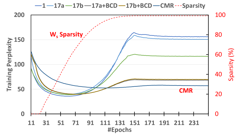
Figure 4: (Best viewed in color) Using the various alternative techniques described in equation 17a - 17b with and without block coordinate descent (BCD), we see that the reliance on $W_{s}$ has reduced. The increase in training perplexity that was visible in Figure 3 has been managed considerably. However, none of the alternative techniques match the training accuracy of CMR.

5.2 CMR for Generalized Doped Structured Matrices

CMR is a phenomenon that we observe when we combine $W_{s}$ with other structured matrices also. We run experiments where we combine a low-rank matrix factorized matrix Kuchaiev & Ginsburg (2017) with a sparse matrix, i.e., the parameter matrix is replaced as:

$$W=W_{lmf}+W_{s},$$ (18)

$$W_{lmf}=B\times C,$$ (19)

where, $B\in R^{M\times d}$, $C\in R^{d\times N}$ and $W_{lmf}\in R^{M\times N}$ and $d<min(M,N)$. We call this method doped LMF. Similarly, we can create doped HMD Thakker et al. (2019) compression method. We show that doping, CMR and CMA are applicable and useful for achieving high-accuracy for doped LMF (HMD) compression method also. Section 6.2 discusses results of compression using doped LMF (HMD) and how they fare against doped KP compression method.

5.3 Training using CMR Dropout

CMR dropout is needed to avoid CMA. However as the $W_{s}$ gets pruned over-time, the need for CMR decreases. In order to verify this, we experiment with 3 different CMR schedules:

• constant: The CMR dropout value remains constant throughout the training run

• linDec: This is the linear decrease schedule. We maintain a constant CMR dropout value for the first few epochs. We start decreasing the CMR value linearly to zero as soon as we start pruning $W_{s}$. We linearly decrease CMR to zero. The number of steps in which the CMR decreases to zero is equal to number of steps taken to prune $W_{s}$ to the required sparsity values. Finally, we train the network with no CMR (zero CMR) for a few more epochs.

• expDec: This is the exponential decrease schedule. We maintain a constant CMR dropout value for the first few epochs. We start decreasing the CMR value proportional to the density of the $W_{s}$ matrix as soon as we start pruning $W_{s}$. Once the $W_{s}$ matrix is pruned to the required sparsity value, CMR dropout converges to zero. Finally, we train the network with no CMR (zero CMR) for a few more epochs.

Table 2: Ablation study comparing various CMR dropout schedules (Section 5.3). Schedules that adapt to changing sparsity levels in $W_{s}$ achieve better results than other schedules. Thus, linDec and expDec achieve better Test Perplexity than constant. constant schedule maintains a large dropout value even after most of the weights in $W_{s}$ are pruned away, inhibiting learning.

	Compression	CMR Schedule	Test Ppl.
Baseline	1x	-	82.1
Doped KP	20x	constant	88.5
	20x	expDec	83.6
	20x	linDec	82.9

Results in Table 2 indicate that linDec achieves the best accuracy when compared to other schedules. constant achieves the highest test perplexity value while expDec achieves comparable accuracy to linDec. constant leads to least accuracy as having a CMR dropout after pruning away most of the weights in $W_{s}$ inhibits learning. Thus, schedules that adapt to the sparsity levels of $W_{s}$ generally fare better. This paper uses the linDec schedule for CMR dropout.

6 Results

6.1 Datasets and Benchmarking Methodology

We evaluate the compression technique on networks trained on two different datasets. We train the language models on the Penn Treebank Corpus Marcus et al. (1993). The dataset consists of 929k training words, 73k validation words and 82k test words with a total vocabulary size of 10000. The machine translation network is trained on the English-Vietnamese Translation dataset. The dataset consists of 133k training sentence examples, 1553 sentences in the validation set and 1268 sentences in the test set. The networks were trained using Tensorflow 1.14 platform using 2 Nvidia RTX 2080 GPUs.

We compare networks compressed using DKP with multiple alternatives:

• Pruning: We use the magnitude pruning framework provided by Zhu & Gupta (2017). While there are other possible ways to prune, recent work Gale et al. (2019a) has suggested that magnitude pruning provides state-of-the-art or comparable performance when compared to other pruning techniques Neklyudov et al. (2017); Louizos et al. (2018).

• Low-rank Matrix Factorization (LMF): LMF  Kuchaiev & Ginsburg (2017) expresses a matrix $A\in\mathbb{R}^{m\times n}$ as a product of two matrices $U\in\mathbb{R}^{m\times d}$ and $V\in\mathbb{R}^{d\times n}$, where $d$ controls the compression factor.

• Small Baseline: Additionally, we train a smaller baseline with the number of parameters equal to that of the compressed baseline. The smaller baseline helps us evaluate if the network was over-parameterized.

• Previous state-of-the-art: Additionally, we show results comparing our method with previous state-of-the-art compression results on the same benchmark.

In order to understand the generality of the compression technique, we evaluate and compress 4 different benchmarks across two applications - Language Modeling and Language Translation. They are:

• Medium LM in  Zaremba et al. (2014): The LM consists of 2 LSTM layers with hidden size of 650. The baseline network was trained using a learning rate of 1.0 for 39 epochs with a learning rate decay of 0.8. For regularization we use max grad norm value of 5 and a dropout of 0.5 for all the layers.

• Large LM in  Zaremba et al. (2014): The LM consists of 2 LSTM layers with hidden size of 1500. The baseline network was trained using a learning rate of 1.0 for 55 epochs with a learning rate decay of 0.85. For regularization we use max grad norm value of 10 and a dropout of 0.65 for all the layers.

• RHN LM in  Zilly et al. (2016): We train the RHN network with a depth of 10 layers and hidden size of 830. The input and output weight embedding are tied together.

• En-Vi translation network in  Luong et al. (2017): The model uses 2-layer LSTMs of size 512 units with bidirectional encoder and unidirectional decoder, embedding of dimension 512 and an attention layer. The network is trained using a learning rate of 1.0, using a dropout value of 0.2 and gradient norm value of 5.0.

For all of the above networks we compress the LSTM layers in the network, unless stated otherwise. We compare the accuracy of the compressed networks and identify the compression method that achieves the lowest preplexity (highest accuracy). The hyperparameters of the compressed network can be found in Appendix B. We also measure the number of operations required to execute the compressed network and the wall-clock inference run-time of the compressed network on an embedded device.

Table 3: Medium LM LSTM results demonstrate that doping is beneficial when applied to structured compression techniques, such as KP, LMF and HMD shown here. Doped structured matrix compression technique outperforms traditional structured matrix compression (w/o doping). Amongst the different structured matrices, KP outperforms LMF and HMD, due to the higher rank of KP structure. Additionally, the results also indicate that doped structured matrix trained without CMR do no achieve good accuracy due to CMA, thus indicating that CMA and CMR is a phenomenon unique to other structured matrices also.

Method	Compression	Test Perplexity
		Conventional	Doped
Baseline	1x	82.1	-
KP (no CMR)	20x	89.1	93.3
KP w/ CMR	20x	89.1	82.9
LMF (no CMR)	20x	103.4	107.1
LMF w/ CMR	20x	103.4	89.2
HMD (no CMR)	20x	98.7	104.8
HMD w/ CMR	20x	98.7	87.4

6.2 Impact of doping structured matrices

Doping is applicable to a variety of structured matrices. We applied doping to low-rank matrix factorization (doped LMF) technique, HMD Thakker et al. (2019) (doped HMD) and kronecker product (doped KP), using the CMR training method. Table 3 summarizes the results for standard and doped structured matrices, trained with and without CMR. At the same compression ratios, doped structured matrix compression outperforms standard structured matrix compression by a margin of 14% or more. This shows that doping, CMA and CMR are generally applicable to structured matrices also, opening opportunities for development and exploration of a broad range of doped structured compression methods.

The results show that the structured matrix used has a significant influence on the final accuracy. Overall, we found a strong correlation between the rank of the structured matrix and the test perplexity results of the doped Structured Matrices. Doping KP matrices leads to superior accuracy than doping LMF and HMD structures. The KP structured matrix has an order of magnitude higher rank than that of LMF and HMD Thakker et al. (2019a) for same number of parameters. Therefore,the KP matrix is far more expressive than an LMF or HMD equivalent, resulting in superior performance. This makes KP a better structure to combine with doping. Similarly, HMD has double the rank of the matrix than one decomposed using LMF for the same number of parameters, thus doped HMD has a better perplexity than doped LMF.

6.3 Compression using Doped Kronecker Product matrices

Section 6.2 showed that doped KP compression outperforms other doped structured matrix based compression techniques by a large margin. In this section we will compare this compression technique with other strong alternatives on a wide variety of benchmarks.

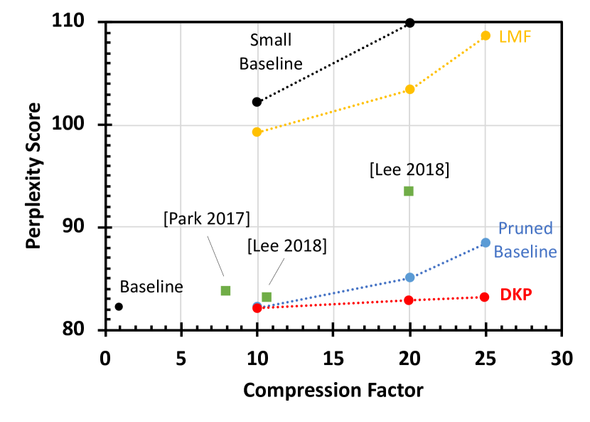
Figure 5: Medium LM at various compression factors. The baseline model defines $1\times$ compression. Doped KP is compared with pruning, LMF (Kuchaiev & Ginsburg (2017)), a smaller baseline (SB), and previous published results on this benchmark Park et al. (2017); Lee & Kim (2018); Lee et al. (2018).

Table 4: Large LM results show that doped KP has the best perplexity at high compression factors, compared to previous work.

Method	Compression	Test Perplexity
Baseline Model	$1\times$	78.3
Wen et al. (2018)	$9.83\times$	78.6
Wen et al. (2020)	$10.71\times$	78.1
Zhu & Gupta (2017)	$20\times$	83.4
Doped KP (This work)	$20\times$	78.5

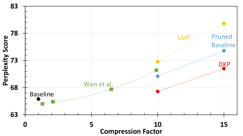
Figure 6: RHN LM at various compression factors. The baseline model defines $1\times$ compression. Doped KP is compared with pruning, LMF (Kuchaiev & Ginsburg (2017)), and previous published results on this benchmark Wen et al. (2018).

Table 5: Compressing a more regularized Large LM regularized using doped KP. We use weight-tying regularization that serves dual purpose of compressed word embedding representation and more regularized network. The results indicate that doped KP can compress a more regularized version of Large LM.

Network	Compression Factor		Perplexity
	Word Embeddings	LSTM Layers
Large LM	1x	1x	78.3
+Weight Tying	2x	1x	73.8
+Doped KP	2x	15x	76.2

Table 6: Results of Compression of a GNMT network

Method	Compression	BLEU Score
Baseline Model	1x	25.5
Pruned Baseline	15x	24.2
LMF	15x	22.8
Small Baseline	15x	23.1
Doped KP	15x	24.9

6.3.1 Medium and Large LM in Zaremba et al. (2014)

Figure 5 shows the Medium LM doped KP results at multiple compression factors, compared with pruned baselines (Zhu & Gupta (2017)), LMF (Kuchaiev & Ginsburg (2017)), and a small baseline with reduced layer sizes. We also include recently published results for the same LMs. As shown, doped KP outperforms all traditional compression techniques known at $20\times$ compression factors and beyond. These models have $W_{s}$ sparsity of $95\%$ or higher. Doped KP achieves 6% better accuracy than pruning and 23.3% better accuracy than LMF for $25\times$ compression factor. Additionally, doped KP outperforms all previously published results, with $2.4\times$ higher compression at the same perplexity as previous best result Lee & Kim (2018).

Table 4 shows the large LM model compressed using doped KP at 25$\times$ compression. Doped KP consistently outperforms both standard techniques and previous work. We improve the state-of-the art, almost doubling ($1.8\times$) the compression at comparable accuracy Wen et al. (2020).

Table 7: Overview of the results highlighting the compressing abilities of doped KP method across a variety of benchmarks. Speed-up over baseline is measured by running the network on a Raspberry Pi 4 board using Eigen C++ Library.

Benchmark	Compression Technique	Perplexity/ BLEU score	Compression Factor	MAC Reduction	Speed-up on commodity hardware
Medium LM	Baseline	82.1	1x	1x	1x
	Lee et al. (2018)	83.1	10x	Not Reported	NAa
	Ours (Doped KP)	83.2	25x	7.41x	4.06x
Large LM	Baseline	78.3	1x	1x	1x
	Wen et al. (2020)	78.1	10.71x	7.48x	14.7x
	Ours (Doped KP)	78.5	20x	5.64x	5.49x
RHN	Baseline	65.9	1x	1x	1x
	Wen et al. (2018)	71.2	10x	5.3x	10.7x
	Ours (Doped KP)	71.1	15x	5.79x	5.34x
GNMT	Baseline	25.5	1x	1x	1x
	Zhu & Gupta (2017)	24.9	10x	10x	3.3x
	Ours (Doped KP)	24.9	15x	6.12x	2.55x

• Previous state-of-the-art (Lee et al. (2018)) cannot be implemented on commodity hardware.

Impact of additional regularization: We wanted to understand whether adding more regularization to the previous models negatively impacted the conclusions in the previous section. In order to do that, we regularized the Large LM using weight tying regularization Inan et al. (2016). Weight Tying (WT) ties the input and output word embeddings of a LM resulting in a smaller network with better generalization. As shown in Table 5, WT compresses the word embeddings by $2\times$ while simultaneously improves the perplexity of the Large LM by 4.5 points when compared to the baseline. Doped KP can further compress the network by $15\times$ with minor impact on perplexity score.

6.3.2 Recurrent Highway Networks (RHN)

We also tested Doped KP compression of a more recent and more heavily regularized LM by Zilly et al. (2016). Figure 6 shows the results of these experiments. As shown in the figure, doped KP can compress the RHN network by $10\times$ with only minor degradation in perplexity score. Additionally, doped KP achieves 1.5$\times$ more compression than previous state-of-the-art compression technology while achieving similar perplexity.

6.3.3 Compressing a Language Translation Network

To understand whether doped KP can be used to compress applications beyond LMs, we compress an English-Vietnamese translation network from Luong et al. (2017). Results in Table 6 show that doped KP can achieve better accuracy than other traditional compression techniques.

6.3.4 Compressing an Intent Detection Network

Using doping, we are able to compress the Intent Detection network Liu & Lane (2016) trained on the ATIS dataset by 10 $\times$, with 0.7% loss in baseline accuracy (97.65%). Pruning the baseline network to a compression factor of 10$\times$ leads to 1.3% loss in baseline accuracy, while LMF leads to 4.2% loss in baseline accuracy.

6.3.5 Impact on Op count and Inference run-time

Table 7 shows the multiply-accumulate operation (MAC) reduction achieved by the networks discussed in this paper for various compression factors. Doped KP achieved near iso-accuracy at $25\times$ compression for the Medium LM, $20\times$ for the Large LM, $15\times$ for GNMT and $10\times$ for RHN. These compression factors correspond to $7.41\times$, $5.64\times$, $6.12\times$ and $5.79\times$ reduction in MAC operations required to execute the LSTM layers of the network.

To measure the wall-clock inference run-time, we implement the compressed network on a Raspberry Pi 4 board Foundation (2009). The borad has Arm Cortex A-72 processor and the networks were implemented using Eigen C++ library Guennebau & Jacob (2009). As shown in Table 7, doped KP compressed networks not only achieve MAC reduction, but also achieves $2.5\times-5.5\times$ inference speed-up.

7 Doped Quantized Network

In general, the doping technique introduced in our paper should apply to any models that use fully connected layers and convolutions. Therefore, in addition to LSTMs, it should also be applicable to MLPs, transformers and CNNs. To demonstrate this, we ran further experiments to apply doping to a quantized AlexNet CNN Krizhevsky et al. (2012) trained on the ImageNet dataset Deng et al. (2009). To do this, we first aggressively quantized the weights in an AlexNet model to 2-bits, which leads to a top-1 accuracy of 50.1%. Next, we doped the network with 1% of FP32 values. We found that this tiny level of doping increases the accuracy by 3.1% to 53.1%. Although this is a preliminary result, we believe it indicates that doping (i.e., the addition of sparse additive matrices) can be useful for CNNs, as well as the LSTMs studied in our paper. It further shows that doping can generalize to structures beyond those discussed in the paper.

8 Limitation and Future Work

In common with many other structured matrix approaches, Doped KP currently introduces a 2-3x training slowdown. This is due to (a) the additional memory required for the sparse matrix (which is initially dense before pruning), and (b) the lack of efficient KP GPU kernels (for both forward- and back-propagation). This training time limitation has so far prevented us from applying doping to big models and big datasets. We believe that (a) could potentially be addressed by the use of second order approximation methods Wu et al. (2019); Dong et al. (2020b). These methods can help identify locations in the structured matrix that are stuck in sub-optimal minima and might benefit from a non-zero value in an equivalent location in the sparse matrix. This might allow us to learn the sparse matrix directly, without the need to prune down from a dense matrix. Additionally, (b) can be avoided by developing specialized GPU kernels for structured matrices. Recently, Dong et al. (2020a) showed how to develop such kernels for block circular matrices, another popular structured matrix. We leave the training time challenge for future work.

9 Conclusion

This paper introduces doping, a technique to improve accuracy of networks compressed using structured matrices like the Kronecker product (KP). Doping introduces an additional additive matrix to the the KP matrices, which we force to be very sparse during training. To train high accuracy networks with large compression factors, doped structured matrices need to over-come co-matrix adaptation (CMA) using the co-matrix regularization (CMR). Doped structured matrices trained using CMR and CMA can train to higher accuracy at larger compression factors than using the structured matrix alone, while achieving better compression factors than previous state-of-the-art compression technique. Specifically, doped KP lead to $10\times-25\times$ with minor loss in accuracy while improving the compression factor of previous state-of-the-art by $1.3\times-2.4\times$. These results were collected by evaluating 4 different NLP application in the domain of language modeling and language translation. Additionally, doped KP compressed network can be deployed on commodity hardware achieving inference speed-up of $2.5-5.5\times$ over baseline.

Appendix A Impact of the dimensions of B and C matrices in $W_{k}$

Table 8: Impact of the choice of different KP compression methodology used for $W_{k}$ matrix. In this paper we follow the methodology in Thakker et al. (2019a). The results of this ablation study compare this choice with various alternatives discussed in Thakker et al. (2019a). For overall compression of $10\times$, we can either start from a $338\times$ KP compressed method and add a $W_{s}$ matrix with $9\%$ non-zero values ( $9\%$ doping) or start from one of the other alternative points and vary the amount of doping. The former follows the methodology used in this paper, while the later describes alternative methodologies that could have been followed. These results validate our initial choice of KP compression for $W_{k}$ and show that the methodology followed in this paper is optimal.

Methodology	KP Compre- ssion	Doping %	Overall Compre- ssion	Test Ppl.
Alternative 1	10$\times$	0%	10$\times$	97.4
Alternative 2	20$\times$	4.5%	10$\times$	91.7
Alternative 3	40$\times$	7%	10$\times$	86.8
This Paper	338$\times$	9%	10$\times$	82.1

Section 3.1 discussed the various choices for the dimension of $B$ and $C$ matrices to express $W_{k}$. For example, if $\boldsymbol{W_{k}}$ is of size 100$\times$100, B and C can be of size $2\times 50and50\times 2$ each or $10\times 10and10\times 10$ each. In this paper, we use the methodology proposed in Thakker et al. (2019a) to identify the configuration of $B$ and $C$ matrix that achieves maximum compression while still preserving the rank of the matrix after compression. Their results indicate that this methodology leads to better accuracy than others. We run a study to validate whether their assumption is applicable to Doped KP networks and thus to validate our initial choice for setting up the compression problem in section 3.1. Table 8 shows the results for this ablation study. The various rows in the table indicate the various methodologies for KP compression and ways to achieve 10$\times$ compression using them. For example the last row shows that using the methodology in this paper, we can start with a $W_{k}$ matrix that is compressed by $338\times$ and add a $W_{s}$ matrix with $9\%$ non-zero parameters ($9\%$ doping) to achieve $10\times$ overall compression. The second last row starts with one of the alternative KP compression methods that compresses the $W_{k}$ matrix by $40\times$ and dopes $7\%$ parameters in the $W_{s}$ matrix to achieve an overall compression of $10\times$. The results validate the choices made in the paper. For iso-compression, doping on top of a matrix compressed using KP compression methodology in Thakker et al. (2019a) achieves least perplexity score when compared to doping on top of a matrix compressed using alternative KP compression methodologies.

Appendix B Hyper-parameters

Table 9: Large LM Hyper-parameters

Large LM Hyper-parameters		Baseline	20x compressed network
size(W)		6000x3000
size(Wk)		NA	52x65 50x20
sparsity(Ws)		NA	96.60%
Initial LR		1	0.3
LR decay		0.85	0.96
#Epochs		55	100
LR Decay Start Epoch		10	15
CMR		NA	0.7
L2 Regularization		0.0001	0.0001
Max Grad Norm		5	5
Dropout		0.65	0.65
Sparsity Schedule	Epoch # during start of pruning	NA	20
	Epoch # during end of pruning	NA	90

Table 10: GNMT Hyper-parameters

		Baseline	Compressed
Attention Type		scaled luong
dropout		0.2	0.2
encoder type		bidirectional
learning rate		1.0	1
max grad norm		5	5
size(W)		2048x1024
size(Wk)		NA	32x8 64x128
sparsity(Ws)		NA
src max len		50	50
beam width		10	10
#TrainSteps		12000	20000
LR Schedule		luang234
Sparsity Schedule	Epoch # during start of pruning	2000	130000
	Epoch # during end of pruning	2000	130000

Table 11: Medium LM hyperparameters

Medium LM Hyper-parameters		Baseline	10x compressed network	20x compressed network	25x compressed network
size(W)		2600x1300
size(Wk)		NA	52x65 & 50x20
sparsity(Ws)		NA	91.10%	95.30%	96.30%
Initial LR		1	0.3	0.3	0.3
LR decay		0.8	0.96	0.96	0.96
#Epochs		40	100	100	100
LR Decay Start Epoch		5	15	15	15
CMR		NA	0.7	0.7	0.7
L2 Regularization		0.0001	0.0001	0.0001	0.0001
Max Grad Norm		5	5	5	5
Dropout		0.5	0.5	0.5	0.5
Sparsity Scedule	Epoch # during start of pruning	NA	20	20	20
	Epoch # during end of pruning	NA	90	90	90

References

- Acharya et al. (2019) Acharya, A., Goel, R., Metallinou, A., and Dhillon, I. Online embedding compression for text classification using low rank matrix factorization. In Proceedings of the AAAI Conference on Artificial Intelligence, volume 33, pp. 6196–6203, 2019.
- Banbury et al. (2021) Banbury, C., Zhou, C., Fedorov, I., Navarro, R. M., Thakker, U., Gope, D., Reddi, V. J., Mattina, M., and Whatmough, P. N. Micronets: Neural network architectures for deploying tinyml applications on commodity microcontrollers, 2021.
- Bradbury et al. (2016) Bradbury, J., Merity, S., Xiong, C., and Socher, R. Quasi-recurrent neural networks. CoRR, abs/1611.01576, 2016. URL http://arxiv.org/abs/1611.01576.
- Campos et al. (2018) Campos, V., Jou, B., Giró-i Nieto, X., Torres, J., and Chang, S.-F. Skip rnn: Learning to skip state updates in recurrent neural networks. In International Conference on Learning Representations, 2018.
- Chen et al. (2018) Chen, T., Lin, J., Lin, T., Han, S., Wang, C., and Zhou, D. Adaptive mixture of low-rank factorizations for compact neural modeling. Advances in neural information processing systems (CDNNRIA workshop), 2018. URL https://openreview.net/forum?id=B1eHgu-Fim.
- Cheng et al. (2015) Cheng, Y., Yu, F. X., Feris, R. S., Kumar, S., Choudhary, A., and Chang, S. An exploration of parameter redundancy in deep networks with circulant projections. In 2015 IEEE International Conference on Computer Vision (ICCV), pp. 2857–2865, Dec 2015. doi: 10.1109/ICCV.2015.327.
- Deng et al. (2018) Deng, C., Liao, S., Xie, Y., Parhi, K. K., Qian, X., and Yuan, B. Permdnn: Efficient compressed dnn architecture with permuted diagonal matrices. In 2018 51st Annual IEEE/ACM International Symposium on Microarchitecture (MICRO), pp. 189–202, 2018.
- Deng et al. (2009) Deng, J., Dong, W., Socher, R., Li, L., Kai Li, and Li Fei-Fei. Imagenet: A large-scale hierarchical image database. In 2009 IEEE Conference on Computer Vision and Pattern Recognition, pp. 248–255, 2009. doi: 10.1109/CVPR.2009.5206848.
- Dennis et al. (2019) Dennis, D., Acar, A., Vikram, M., Simhadri, H., Saligrama, V., and Jain, P. Sharnn: A method for accurate time-series classification on tiny devices. In Proceedings of the Thirty-second Annual Conference on Neural Information Processing Systems (NeurIPS), 2019. URL all_papers/DennisAVSSJ19.pdf. slides/DennisAVSSJ19.pdf.
- Ding et al. (2017a) Ding, C., Liao, S., Wang, Y., Li, Z., Liu, N., Zhuo, Y., Wang, C., Qian, X., Bai, Y., Yuan, G., Ma, X., Zhang, Y., Tang, J., Qiu, Q., Lin, X., and Yuan, B. Circnn: Accelerating and compressing deep neural networks using block-circulant weight matrices. In Proceedings of the 50th Annual IEEE/ACM International Symposium on Microarchitecture, MICRO-50 ’17, pp. 395–408, New York, NY, USA, 2017a. Association for Computing Machinery. ISBN 9781450349529. doi: 10.1145/3123939.3124552. URL https://doi.org/10.1145/3123939.3124552.
- Ding et al. (2017b) Ding, C., Liao, S., Wang, Y., Li, Z., Liu, N., Zhuo, Y., Wang, C., Qian, X., Bai, Y., Yuan, G., Ma, X., Zhang, Y., Tang, J., Qiu, Q., Lin, X., and Yuan, B. Circnn: Accelerating and compressing deep neural networks using block-circulant weight matrices. In Proceedings of the 50th Annual IEEE/ACM International Symposium on Microarchitecture, MICRO-50 ’17, pp. 395–408, New York, NY, USA, 2017b. ACM. ISBN 978-1-4503-4952-9. doi: 10.1145/3123939.3124552. URL http://doi.acm.org/10.1145/3123939.3124552.
- Ding et al. (2018) Ding, C., Ren, A., Yuan, G., Ma, X., Li, J., Liu, N., Yuan, B., and Wang, Y. Structured weight matrices-based hardware accelerators in deep neural networks: Fpgas and asics. In Proceedings of the 2018 on Great Lakes Symposium on VLSI, GLSVLSI ’18, pp. 353–358, New York, NY, USA, 2018. ACM. ISBN 978-1-4503-5724-1. doi: 10.1145/3194554.3194625. URL http://doi.acm.org/10.1145/3194554.3194625.
- Dong et al. (2020a) Dong, S., Zhao, P., Lin, X., and Kaeli, D. Exploring gpu acceleration of deep neural networks using block circulant matrices. Parallel Computing, 100:102701, 2020a. ISSN 0167-8191. doi: https://doi.org/10.1016/j.parco.2020.102701. URL https://www.sciencedirect.com/science/article/pii/S0167819120300909.
- Dong et al. (2020b) Dong, Z., Yao, Z., Arfeen, D., Gholami, A., Mahoney, M. W., and Keutzer, K. Hawq-v2: Hessian aware trace-weighted quantization of neural networks. In Larochelle, H., Ranzato, M., Hadsell, R., Balcan, M. F., and Lin, H. (eds.), Advances in Neural Information Processing Systems, volume 33, pp. 18518–18529. Curran Associates, Inc., 2020b. URL https://proceedings.neurips.cc/paper/2020/file/d77c703536718b95308130ff2e5cf9ee-Paper.pdf.
- Fedorov et al. (2019) Fedorov, I., Adams, R. P., Mattina, M., and Whatmough, P. N. SpArSe: Sparse Architecture Search for CNNs on Resource-Constrained Microcontrollers. In Advances in Neural Information Processing Systems 32, pp. 4978–4990. Curran Associates, Inc., 2019. URL http://papers.nips.cc/paper/8743-sparse-sparse-architecture-search-for-cnns-on-resource-constrained-microcontrollers.pdf.
- Fedorov et al. (2020) Fedorov, I., Stamenovic, M., Jensen, C., Yang, L.-C., Mandell, A., Gan, Y., Mattina, M., and Whatmough, P. N. TinyLSTMs: Efficient Neural Speech Enhancement for Hearing Aids. arXiv preprint arXiv:2005.11138, 2020.
- Foundation (2009) Foundation, R. P. Raspberry pi 4 model b. https://www.raspberrypi.org/products/raspberry-pi-4-model-b/specifications/, 2009. Accessed: 2020-08-10.
- Gale et al. (2019a) Gale, T., Elsen, E., and Hooker, S. The state of sparsity in deep neural networks. CoRR, abs/1902.09574, 2019a. URL http://arxiv.org/abs/1902.09574.
- Gale et al. (2019b) Gale, T., Elsen, E., and Hooker, S. The state of sparsity in deep neural networks. CoRR, abs/1902.09574, 2019b. URL http://arxiv.org/abs/1902.09574.
- Gope et al. (2019) Gope, D., Dasika, G., and Mattina, M. Ternary hybrid neural-tree networks for highly constrained iot applications. In Proceedings of Machine Learning and Systems 2019, pp. 190–200. 2019.
- Gope et al. (2020a) Gope, D., Beu, J., Thakker, U., and Mattina, M. Ternary mobilenets via per-layer hybrid filter banks. In Proceedings of the IEEE/CVF Conference on Computer Vision and Pattern Recognition (CVPR) Workshops, June 2020a.
- Gope et al. (2020b) Gope, D., Beu, J. G., Thakker, U., and Mattina, M. Aggressive compression of mobilenets using hybrid ternary layers. tinyML Summit, 2020b. URL https://www.tinyml.org/summit/abstracts/Gope_Dibakar_poster_abstract.pdf.
- Grachev et al. (2017) Grachev, A. M., Ignatov, D. I., and Savchenko, A. V. Neural networks compression for language modeling. In Shankar, B. U., Ghosh, K., Mandal, D. P., Ray, S. S., Zhang, D., and Pal, S. K. (eds.), Pattern Recognition and Machine Intelligence, pp. 351–357, Cham, 2017. Springer International Publishing. ISBN 978-3-319-69900-4.
- Grachev et al. (2019) Grachev, A. M., Ignatov, D. I., and Savchenko, A. V. Compression of recurrent neural networks for efficient language modeling. Applied Soft Computing, 79:354 – 362, 2019. ISSN 1568-4946. doi: https://doi.org/10.1016/j.asoc.2019.03.057. URL http://www.sciencedirect.com/science/article/pii/S1568494619301851.
- Guennebau & Jacob (2009) Guennebau, G. and Jacob, B. Eigen library. http://eigen.tuxfamily.org/, 2009. Accessed: 2020-08-10.
- Han et al. (2016) Han, S., Mao, H., and Dally, W. J. Deep compression: Compressing deep neural networks with pruning, trained quantization and huffman coding. International Conference on Learning Representations (ICLR), 2016.
- He et al. (2015) He, K., Zhang, X., Ren, S., and Sun, J. Deep residual learning for image recognition. CoRR, abs/1512.03385, 2015. URL http://arxiv.org/abs/1512.03385.
- Huang et al. (2020) Huang, X., Thakker, U., Gope, D., and Beu, J. Pushing the envelope of dynamic spatial gating technologies. In Proceedings of the 2nd International Workshop on Challenges in Artificial Intelligence and Machine Learning for Internet of Things, AIChallengeIoT ’20, pp. 21–26, New York, NY, USA, 2020. Association for Computing Machinery. ISBN 9781450381345. doi: 10.1145/3417313.3429380. URL https://doi.org/10.1145/3417313.3429380.
- Hubara et al. (2016) Hubara, I., Courbariaux, M., Soudry, D., El-Yaniv, R., and Bengio, Y. Binarized neural networks. In Lee, D. D., Sugiyama, M., Luxburg, U. V., Guyon, I., and Garnett, R. (eds.), Advances in Neural Information Processing Systems 29, pp. 4107–4115. Curran Associates, Inc., 2016. URL http://papers.nips.cc/paper/6573-binarized-neural-networks.pdf.
- Hubara et al. (2017) Hubara, I., Courbariaux, M., Soudry, D., El-Yaniv, R., and Bengio, Y. Quantized neural networks: Training neural networks with low precision weights and activations. J. Mach. Learn. Res., 18(1):6869–6898, January 2017. ISSN 1532-4435.
- Inan et al. (2016) Inan, H., Khosravi, K., and Socher, R. Tying word vectors and word classifiers: A loss framework for language modeling. CoRR, abs/1611.01462, 2016. URL http://arxiv.org/abs/1611.01462.
- Krizhevsky et al. (2012) Krizhevsky, A., Sutskever, I., and Hinton, G. E. Imagenet classification with deep convolutional neural networks. In Pereira, F., Burges, C. J. C., Bottou, L., and Weinberger, K. Q. (eds.), Advances in Neural Information Processing Systems, volume 25. Curran Associates, Inc., 2012. URL https://proceedings.neurips.cc/paper/2012/file/c399862d3b9d6b76c8436e924a68c45b-Paper.pdf.
- Kuchaiev & Ginsburg (2017) Kuchaiev, O. and Ginsburg, B. Factorization tricks for LSTM networks. CoRR, abs/1703.10722, 2017. URL http://arxiv.org/abs/1703.10722.
- Kusupati et al. (2018) Kusupati, A., Singh, M., Bhatia, K., Kumar, A., Jain, P., and Varma, M. Fastgrnn: A fast, accurate, stable and tiny kilobyte sized gated recurrent neural network. In Proceedings of the Thirty-first Annual Conference on Neural Information Processing Systems (NeurIPS), pp. 9031–9042, 2018. URL all_papers/KusupatiSBKJV18.pdf. slides/fastgrnn.pdf.
- Lee & Kim (2018) Lee, D. and Kim, B. Retraining-based iterative weight quantization for deep neural networks. CoRR, abs/1805.11233, 2018. URL http://arxiv.org/abs/1805.11233.
- Lee et al. (2018) Lee, D., Kapoor, P., and Kim, B. Deeptwist: Learning model compression via occasional weight distortion. CoRR, abs/1810.12823, 2018. URL http://arxiv.org/abs/1810.12823.
- Lei et al. (2018) Lei, T., Zhang, Y., Wang, S. I., Dai, H., and Artzi, Y. Simple recurrent units for highly parallelizable recurrence. In Proceedings of the 2018 Conference on Empirical Methods in Natural Language Processing, pp. 4470–4481, Brussels, Belgium, October-November 2018. Association for Computational Linguistics. doi: 10.18653/v1/D18-1477. URL https://www.aclweb.org/anthology/D18-1477.
- Li et al. (2019) Li, H., Bhargav, M., Whatmough, P. N., and Philip Wong, H. . On-Chip Memory Technology Design Space Explorations for Mobile Deep Neural Network Accelerators. In 2019 56th ACM/IEEE Design Automation Conference (DAC), pp. 1–6, 2019.
- Liu & Lane (2016) Liu, B. and Lane, I. Attention-based recurrent neural network models for joint intent detection and slot filling. CoRR, abs/1609.01454, 2016. URL http://arxiv.org/abs/1609.01454.
- Liu et al. (2018) Liu, X., Cao, D., and Yu, K. Binarized LSTM language model. In Proceedings of the 2018 Conference of the North American Chapter of the Association for Computational Linguistics: Human Language Technologies, Volume 1 (Long Papers), pp. 2113–2121, New Orleans, Louisiana, June 2018. Association for Computational Linguistics. doi: 10.18653/v1/N18-1192. URL https://www.aclweb.org/anthology/N18-1192.
- Liu et al. (2020) Liu, Z., Whatmough, P. N., and Mattina, M. Systolic Tensor Array: An Efficient Structured-Sparse GEMM Accelerator for Mobile CNN Inference. IEEE Computer Architecture Letters, 19(1):34–37, 2020. doi: 10.1109/LCA.2020.2979965.
- Louizos et al. (2018) Louizos, C., Welling, M., and Kingma, D. P. Learning sparse neural networks through l_0 regularization. In 6th International Conference on Learning Representations, ICLR 2018, Vancouver, BC, Canada, April 30 - May 3, 2018, Conference Track Proceedings. OpenReview.net, 2018. URL https://openreview.net/forum?id=H1Y8hhg0b.
- Luong et al. (2017) Luong, M., Brevdo, E., and Zhao, R. Neural machine translation (seq2seq) tutorial. https://github.com/tensorflow/nmt, 2017.
- Marcus et al. (1993) Marcus, M. P., Marcinkiewicz, M. A., and Santorini, B. Building a large annotated corpus of english: The penn treebank. Comput. Linguist., 19(2):313–330, June 1993. ISSN 0891-2017.
- Mehta et al. (2018) Mehta, S., Koncel-Kedziorski, R., Rastegari, M., and Hajishirzi, H. Pyramidal recurrent unit for language modeling. CoRR, abs/1808.09029, 2018. URL http://arxiv.org/abs/1808.09029.
- Mehta et al. (2019) Mehta, S., Koncel-Kedziorski, R., Rastegari, M., and Hajishirzi, H. Define: Deep factorized input token embeddings for neural sequence modeling, 2019.
- Nagy (2009) Nagy, J. G. Kronecker products. http://www.mathcs.emory.edu/~nagy/courses/fall10/515/KroneckerIntro.pdf, 2009. Accessed: 2020-08-10.
- Neklyudov et al. (2017) Neklyudov, K., Molchanov, D., Ashukha, A., and Vetrov, D. Structured bayesian pruning via log-normal multiplicative noise. In Proceedings of the 31st International Conference on Neural Information Processing Systems, NIPS’17, pp. 6778–6787, Red Hook, NY, USA, 2017. Curran Associates Inc. ISBN 9781510860964.
- Park et al. (2017) Park, E., Ahn, J., and Yoo, S. Weighted-entropy-based quantization for deep neural networks. In 2017 IEEE Conference on Computer Vision and Pattern Recognition (CVPR), pp. 7197–7205, July 2017. doi: 10.1109/CVPR.2017.761.
- Raju et al. (2020) Raju, R., Gope, D., Thakker, U., and Beu, J. Understanding the impact of dynamic channel pruning on conditionally parameterized convolutions. In Proceedings of the 2nd International Workshop on Challenges in Artificial Intelligence and Machine Learning for Internet of Things, AIChallengeIoT ’20, pp. 27–33, New York, NY, USA, 2020. Association for Computing Machinery. ISBN 9781450381345. doi: 10.1145/3417313.3429381. URL https://doi.org/10.1145/3417313.3429381.
- Sanh et al. (2019) Sanh, V., Debut, L., Chaumond, J., and Wolf, T. Distilbert, a distilled version of bert: smaller, faster, cheaper and lighter, 2019.
- Sanh et al. (2020) Sanh, V., Wolf, T., and Rush, A. M. Movement pruning: Adaptive sparsity by fine-tuning, 2020.
- Seo et al. (2018) Seo, M. J., Min, S., Farhadi, A., and Hajishirzi, H. Neural speed reading via skim-rnn. In 6th International Conference on Learning Representations, ICLR 2018, Vancouver, BC, Canada, April 30 - May 3, 2018, Conference Track Proceedings. OpenReview.net, 2018. URL https://openreview.net/forum?id=Sy-dQG-Rb.
- Sindhwani et al. (2015) Sindhwani, V., Sainath, T., and Kumar, S. Structured transforms for small-footprint deep learning. In Cortes, C., Lawrence, N. D., Lee, D. D., Sugiyama, M., and Garnett, R. (eds.), Advances in Neural Information Processing Systems 28, pp. 3088–3096. Curran Associates, Inc., 2015.
- Tao et al. (2019) Tao, J., Thakker, U., Dasika, G., and Beu, J. Skipping rnn state updates without retraining the original model. In Proceedings of the 1st Workshop on Machine Learning on Edge in Sensor Systems, SenSys-ML 2019, pp. 31–36, New York, NY, USA, 2019. Association for Computing Machinery. ISBN 9781450370110. doi: 10.1145/3362743.3362965. URL https://doi.org/10.1145/3362743.3362965.
- Thakker et al. (2019) Thakker, U., Beu, J., Gope, D., Dasika, G., and Mattina, M. Run-time efficient rnn compression for inference on edge devices. In 2019 2nd Workshop on Energy Efficient Machine Learning and Cognitive Computing for Embedded Applications (EMC2), pp. 26–30, 2019.
- Thakker et al. (2019a) Thakker, U., Beu, J. G., Gope, D., Zhou, C., Fedorov, I., Dasika, G., and Mattina, M. Compressing rnns for iot devices by 15-38x using kronecker products. CoRR, abs/1906.02876, 2019a. URL http://arxiv.org/abs/1906.02876.
- Thakker et al. (2019b) Thakker, U., Dasika, G., Beu, J. G., and Mattina, M. Measuring scheduling efficiency of rnns for NLP applications. CoRR, abs/1904.03302, 2019b. URL http://arxiv.org/abs/1904.03302.
- Thakker et al. (2019c) Thakker, U., Fedorov, I., Beu, J. G., Gope, D., Zhou, C., Dasika, G., and Mattina, M. Pushing the limits of rnn compression. ArXiv, abs/1910.02558, 2019c.
- Thakker et al. (2020a) Thakker, U., Beu, J., Gope, D., Dasika, G., and Mattina, M. Rank and run-time aware compression of NLP applications. In Proceedings of SustaiNLP: Workshop on Simple and Efficient Natural Language Processing, pp. 8–18, Online, November 2020a. Association for Computational Linguistics. doi: 10.18653/v1/2020.sustainlp-1.2. URL https://www.aclweb.org/anthology/2020.sustainlp-1.2.
- Thakker et al. (2020b) Thakker, U., Whatamough, P., Mattina, M., and Beu, J. G. Compressing language models using doped kronecker products. CoRR, abs/2001.08896, 2020b. URL https://arxiv.org/abs/2001.08896.
- Thomas et al. (2018) Thomas, A., Gu, A., Dao, T., Rudra, A., and Ré, C. Learning compressed transforms with low displacement rank. In Bengio, S., Wallach, H., Larochelle, H., Grauman, K., Cesa-Bianchi, N., and Garnett, R. (eds.), Advances in Neural Information Processing Systems 31, pp. 9052–9060. Curran Associates, Inc., 2018. URL http://papers.nips.cc/paper/8119-learning-compressed-transforms-with-low-displacement-rank.pdf.
- Tjandra et al. (2017) Tjandra, A., Sakti, S., and Nakamura, S. Compressing recurrent neural network with tensor train. In Neural Networks (IJCNN), 2017 International Joint Conference on, pp. 4451–4458. IEEE, 2017.
- Wen et al. (2020) Wen, L., Zhang, X., Bai, H., and Xu, Z. Structured pruning of recurrent neural networks through neuron selection. Neural Networks, 123:134 – 141, 2020. ISSN 0893-6080. doi: https://doi.org/10.1016/j.neunet.2019.11.018. URL http://www.sciencedirect.com/science/article/pii/S0893608019303776.
- Wen et al. (2018) Wen, W., Chen, Y., Li, H., He, Y., Rajbhandari, S., Zhang, M., Wang, W., Liu, F., and Hu, B. Learning intrinsic sparse structures within long short-term memory. In ICLR 2018 Conference, February 2018. URL https://www.microsoft.com/en-us/research/publication/learning-intrinsic-sparse-structures-within-long-short-term-memory/.
- Whatmough et al. (2018) Whatmough, P. N., Lee, S. K., Brooks, D., and Wei, G. DNN Engine: A 28-nm Timing-Error Tolerant Sparse Deep Neural Network Processor for IoT Applications. IEEE Journal of Solid-State Circuits, 53(9):2722–2731, 2018. doi: 10.1109/JSSC.2018.2841824.
- Whatmough et al. (2019) Whatmough, P. N., Zhou, C., Hansen, P., Venkataramanaiah, S. K., sun Seo, J., and Mattina, M. FixyNN: Efficient Hardware for Mobile Computer Vision via Transfer Learning. In 2nd Conference on Systems and Machine Learning (SysML), 2019.
- Wu et al. (2019) Wu, L., Wang, D., and Liu, Q. Splitting steepest descent for growing neural architectures. In Advances in Neural Information Processing Systems, volume 32. Curran Associates, Inc., 2019. URL https://proceedings.neurips.cc/paper/2019/file/3a01fc0853ebeba94fde4d1cc6fb842a-Paper.pdf.
- Yu et al. (2017) Yu, A. W., Lee, H., and Le, Q. Learning to skim text. In Proceedings of the 55th Annual Meeting of the Association for Computational Linguistics (Volume 1: Long Papers), pp. 1880–1890, Vancouver, Canada, July 2017. Association for Computational Linguistics. doi: 10.18653/v1/P17-1172. URL https://www.aclweb.org/anthology/P17-1172.
- Zaremba et al. (2014) Zaremba, W., Sutskever, I., and Vinyals, O. Recurrent neural network regularization. CoRR, abs/1409.2329, 2014. URL http://arxiv.org/abs/1409.2329.
- Zhou et al. (2015) Zhou, S., Wu, J., Wu, Y., and Zhou, X. Exploiting local structures with the kronecker layer in convolutional networks. CoRR, abs/1512.09194, 2015. URL http://arxiv.org/abs/1512.09194.
- Zhu & Gupta (2017) Zhu, M. and Gupta, S. To prune, or not to prune: exploring the efficacy of pruning for model compression. arXiv e-prints, art. arXiv:1710.01878, October 2017.
- Zhu et al. (2019) Zhu, Y., Mattina, M., and Whatmough, P. N. Mobile Machine Learning Hardware at ARM: A Systems-on-Chip (SoC) Perspective. In 1st Conference on Systems and Machine Learning (SysML), 2019.
- Zilly et al. (2016) Zilly, J. G., Srivastava, R. K., Koutník, J., and Schmidhuber, J. Recurrent highway networks. CoRR, abs/1607.03474, 2016. URL http://arxiv.org/abs/1607.03474.