A Statistical Relational Approach to
Learning Distance-based GCNs

Abstract

We consider the problem of learning distance-based Graph Convolutional Networks (GCNs) for relational data. Specifically, we first embed the original graph into the Euclidean space $\mathbb{R}^{m}$ using a relational density estimation technique thereby constructing a secondary Euclidean graph. The graph vertices correspond to the target triples and edges denote the Euclidean distances between the target triples. We emphasize the importance of learning the secondary Euclidean graph and the advantages of employing a distance matrix over the typically used adjacency matrix. Our comprehensive empirical evaluation demonstrates the superiority of our approach over $\mathbf{12}$ different GCN models, relational embedding techniques and rule learning techniques.

Introduction

Statistical Relational Learning (SRL) (Getoor and Taskar 2007; Raedt et al. 2016) combines the power of probabilistic models to handle uncertainty with the ability of relational models to faithfully capture the rich domain structure. One of the key successes of these models lie in the task of knowledge base population, specifically, link prediction and node classification. While successful, most methods make several simplifying assumptions – presence of supervision in the form of labels, closed-world assumption, presence of only binary relations and most importantly, in many cases, the presence of hand-crafted domain rules.

We go beyond these assumptions and inspired by the recent success of Graph Convolutional Networks (GCNs) (Defferrard, Bresson, and Vandergheynst 2016; Kipf and Welling 2017), develop a new framework for relational GCNs. This framework has two key steps: (1) create a secondary Euclidean graph from the original graph by learning rules from one-class data, i.e., from the positive and negative annotations of the target relation separately. The next step is to convert these rules into observed features i.e., instantiates and counts the number of times the rules fire and computes the distance matrix, and (2) finally, it trains a GCN using the observed features and the distance matrix. For the first step, our method employs a one-class density estimation method that employs a tree-based distance metric to learn relational rules iteratively. Hence, we call the framework as Relational Density Distance-based GCN (RD²GCN). Since the two different steps of learning the relational rules and training the GCN employ the same set of positive examples, a richer representation of the combination of the attributes, entities and their relations is obtained. While previous methods used the features as the observed layer, RD²GCN uses the rules as the observed layer. This has the added advantage of the latent layer being richer – it combines the instantiations of first-order rules themselves allowing for a richer representation. We hypothesize and show empirically that this is specifically useful when employed on link prediction tasks. Although work exists on generating similarity graphs using GNNs (Bai et al. 2018, 2019; Li et al. 2019), ours is the first method to use GCNs on induced similarities graphs allowing for use of richer features.

We make a few key contributions: (1) We develop the first relational GCN capable of utilizing the different densities of the data separately. (2) Going beyond using carefully designed hand-crafted rules, our method learns rules automatically to construct a secondary graph and constructs the GCN. These two steps are conditioned on the required task and allow for a better classifier and thus can learn with smaller data. (3) RD²GCN can handle arbitrary relations – not simple binary relations that most methods use. Given that our base learner employs a logic learner, the relations can be $n-$ary. (4) We show the advantages of using distance matrices and Euclidean distance to construct the distance matrix. Our evaluation across $\mathbf{12}$ different baselines and $3$ different data sets clearly demonstrates the effectiveness of RD²GCN.

Background and Related work

Notations:

A (logical) predicate is of the form $\mathcal{R}(t_{1},\dots,t_{k})$ where $\mathcal{R}$ is a relation and the arguments $t_{i}$ are entities. A substitution is of the form ${\bm{\theta}}=\{\langle l_{1},\dots,l_{k}\rangle/\langle t_{1},\dots,t_{k}\rangle\}$ where $l_{i}$s are logical variables and $t_{i}$s are terms. A grounding of a predicate with variables $l_{1},\dots,l_{k}$ is a substitution $\{\langle l_{1},\dots,l_{k}\rangle/\langle L_{1},\dots,L_{k}\rangle\}$ mapping each of its variables to a constant in the domain of that variable. A knowledge base $\mathcal{B}$ consists of (1) entities: a finite domain of objects $\mathcal{O}$, (2) relations: a set of predicates describing the attributes and relationships between objects $\in\mathcal{O}$, and (3) an interpretation assigning a truth value to every grounding.

Relational Density Estimation:

A common issue in many real-world relational knowledge bases is that only true instances of any relation(s) are labeled while the false instances are not explicitly identified. Consequently closed-world assumption is applied to sample negative instances. While reasonable, this is a strong assumption particularly when the number of positively labeled examples $\ll$ negatively labeled examples. In the relational one-class classification (Khot, Natarajan, and Shavlik 2014) method, given a set of labeled examples, a distance measure is used to perform one-class classification, which involves two levels of combinations: tree-level due to learning multiple trees and instance-level due to the predicates containing variables and different instances for each target. For example, in learning advisedBy(S,P) the first tree could consider the courses and the second could consider the publications. The tree-level combining function combines the results from these two trees. Now the student could potentially publish several papers, or register in multiple courses and inside each tree, these different instances are combined using the instance level combining function (Jaeger 2007; Natarajan et al. 2008). In the tree-level distance computation, the distance between the current unlabeled example $u$ is calculated from a labeled example in all the learned first-order trees. Now the final distance is simply the weighted combination of the individual tree-level distances: $D(l_{1},\,u)=\sum_{i}\,\beta_{i}\,d_{i}(l_{1},u)$ where $\beta_{i}$ is the weight of the $i^{th}$ tree and $\sum_{i}\beta_{i}=1,\beta_{i}\geq 0$. These tree distances are then combined to get an overall distance between the current example and all the labeled examples $l_{j}$, $E(u\not\in\texttt{class})\,=\,\sum_{j}\,\alpha_{j}D(l_{j},\,u)$, where $\alpha_{j}$ is the weight of the labeled example $l_{j}$ and $\sum\alpha_{j}=1,\alpha_{j}\geq 0$.

Knowledge Graph Embeddings (KGEs):

Recently, several successful methods for learning embeddings of large knowledge bases have been developed (Wang et al. 2017; Cai, Zheng, and Chang 2018). Several of these approaches such as TransE (Bordes et al. 2013), TransH (Wang et al. 2014), TransG (Xiao, Huang, and Zhu 2016) and KG2E (He et al. 2015), to name a few, can be grouped into translational distance models that focus on minimizing a distance based function under some constraints or using regularizing factors between entities and relations. More recent approaches extend these translation approaches by embedding the knowledge graphs into more complex spaces such as the hyperbolic space (Balazevic, Allen, and Hospedales 2019; Kolyvakis, Kalousis, and Kiritsis 2019) and the hypercomplex space (Zhang et al. 2019; Sun et al. 2019). Another important class of approaches such as RESCAL (Nickel, Tresp, and Kriegel 2011), DistMult (Yang et al. 2015), TuckER (Balažević, Allen, and Hospedales 2019b), HypER (Balažević, Allen, and Hospedales 2019a) and HolE (Nickel, Rosasco, and Poggio 2016) focus on various compositional operators for the entities and relations in the knowledge graph.

Graph Convolutional Networks (GCNs):

Graph Convolutional Networks (GCNs) (Kipf and Welling 2017) generalize convolutional neural network models to graph-structured data sets where each convolution layer in the GCN applies a graph convolution i.e. a spectral filtering of the graph signal (the feature matrix of the graph) via the Graph Fourier Transform. The main reason behind the success of GCNs is that they exploit two key types of information: node feature descriptions ($x_{i}$) and node neighborhood structure (captured through the adjacency matrix $\mathcal{A}$ of the graph). While successful, GCNs cannot directly be applied on multi-relational data/networks and require propositionalization techniques. Consequently, relational GCNs (Schlichtkrull et al. 2018) construct a latent representation of the entities explicitly and a tensor factorization then exploits these representations for the prediction tasks. We take an alternative approach based on a successful SRL approach  (Khot, Natarajan, and Shavlik 2014; Lao and Cohen 2010) to develop novel combinations of the entities and their relationships to construct richer latent representations. As we demonstrate empirically, this leads to superior predictive performance. In addition, the use of relational rules as the observed layer of the GCN makes them more interpretable/explainable than the tensor factorization approach.

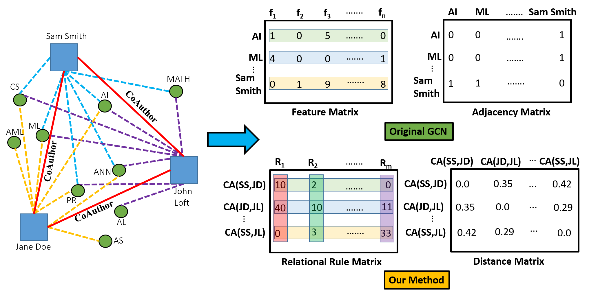
Figure 1: Difference between GCN (Kipf and Welling 2017) and our method with an example input graph. Here, CA is the CoAuthor relation to be predicted. The relational rule matrix is obtained by counting the number of satisfied groundings of the obtained first-order rules (R₁ - R_m) wrt the query variables and is a richer representation of the graph structure.

Relational Density Distance-based GCNs

Direct application of GCNs cannot fully exploit the inherent structures inside a multi-relational graph. Consequently, they need significant engineering to construct the propositionalized features. Motivated by this, we propose a principled extension to the GCN that models large multi-relational networks faithfully. While a recent work R-GCN (Schlichtkrull et al. 2018) extends GCNs to relational domains, it is still limited to graphs represented as (subject; predicate; object) triples and requires multiple adjacency matrices for handling multi-relational data. We propose a novel and a more general approach that is not limited by assumptions about the multi-relationality of the data and can handle general multi-graphs and hypergraphs without loss of information. We can now formally define our model and its components.

Definition 1 (Secondary Euclidean Graph).

A secondary Euclidean graph consists of a set of vertices and edges where the vertices correspond to the query variable in the relational data set and the edges constitute the Euclidean distance between each pair of vertices.

Definition 2 (RD²GCN).

Given a knowledge base/relational graph $\mathcal{B}$ and a function $\phi:\mathcal{B}\mapsto\mathbb{R}^{m}$, such that $\phi$($\mathbb{B}$) = $\mathfrak{E}\in\mathbb{R}^{m}$, RD²GCN $\mathfrak{G}$ is a graph convolutional network defined over $\mathfrak{E}$ and $Euc(\mathfrak{E})$ i.e. the secondary Euclidean graph.

Definition 3 (Relational Rule Matrix).

A relational rule matrix $\mathcal{X}$ contains the node feature descriptors $x_{i}\in\mathfrak{E}$ for a Euclidean graph.

Definition 4 (Distance Matrix).

A distance matrix $\mathcal{D}$ contains the euclidean distances between the node feature descriptors $\in\mathcal{X}$ such that $Euc(\mathfrak{E})\in\mathcal{D}$.

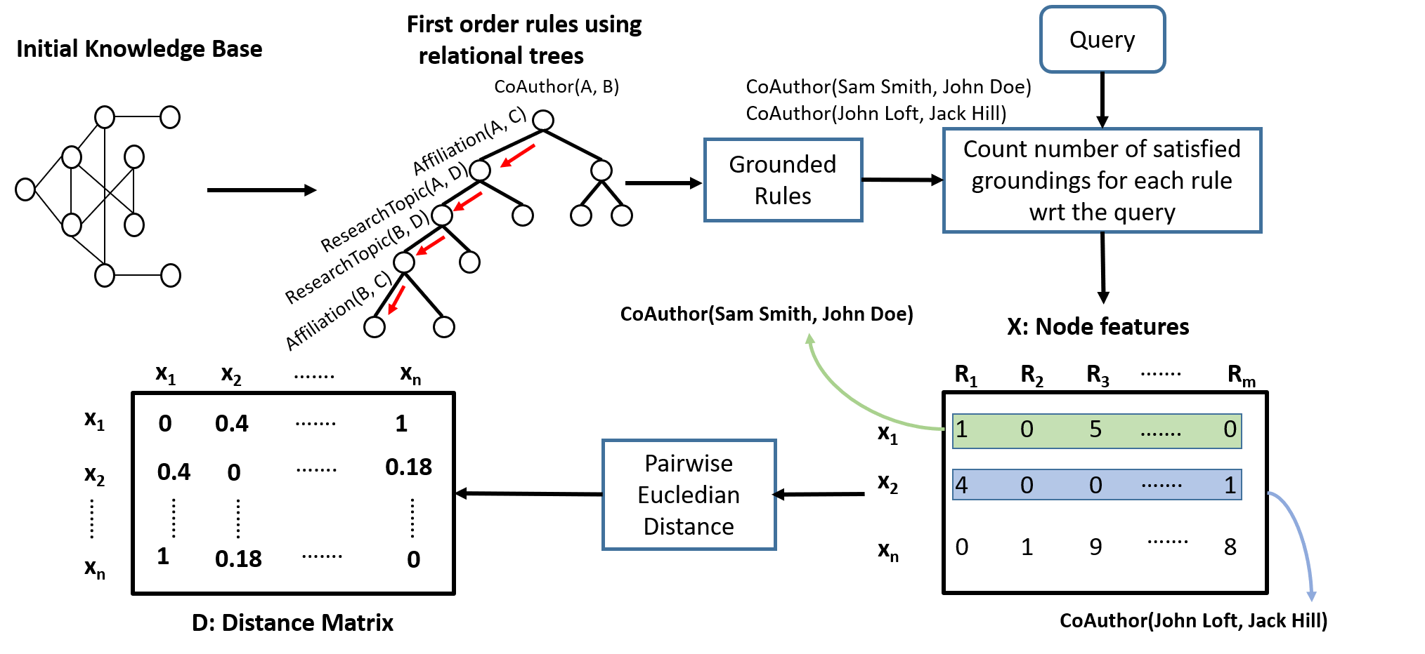
Figure 2: Relational Rule Matrix $\mathcal{X}$ and Distance Matrix $\mathcal{D}$ construction for RD²GCN. First-order rules are learned from the given knowledge bases which are then grounded and satisfied groundings are counted to form $\mathcal{X}$.

Given a knowledge base $\mathcal{B}$, we first learn a set of first-order rules that captures the relations between the domain predicates. The intuition is that these first-order rules can be viewed as higher-order features that connect entities and their attributes. Particularly, when learned for a specific classification task, these features can be both predictive and informative. Given that they are typically conjunctions of relational features (attributes of entities and relationships), they have the added advantage of being interpretable. Our hypothesis, that we verify empirically is that these rules can potentially yield richer latent representations than a relational GCN that simply uses the entity and relationship information. Our key contribution is a two-step process of constructing the link prediction problem as a prediction problem in a secondary Euclidean graph where vertices correspond to target triple rather than individual entities. We learn a relational rule matrix and then build a distance matrix to use for GCN-computations (see Figure 1).

Embedding Original Graph to $\mathbb{R}^{m}$: Creating a Euclidean Graph

We now outline the required steps to embed the original graph to a Euclidean space $\mathbb{R}^{n}$ thereby creating a secondary Euclidean graph. The nodes of the Euclidean graph consists of the target triple with the node features forming the relational rule matrix $\mathcal{X}$ and the edges connecting the nodes are the Euclidean distances thus forming the distance matrix $\mathcal{D}$. It is clear from def. 1-4 that we just need $\mathcal{X}$ and $\mathcal{D}$ to represent a secondary Euclidean graph. Figure 2 shows the construction of $\mathcal{X}$ and $\mathcal{D}$.

Step 1: Rule Learning using Density Estimation: Inspired by the success of learning only from positive examples in relational domains (Khot, Natarajan, and Shavlik 2014), we learn first-order rules using relational density estimation (which forms $\phi$ in def 2) and learn from both the positive and negative examples separately. The intuition behind using a density estimation method is that learning first-order rules for positive and sampled negative examples independently can result in better utilization of the search space thereby (potentially) learning more discriminative features. Figure 3 shows an example of learning such discriminative features for a “Co-Author” data set. The density estimation approach uses a tree-based distance measure that iteratively introduces newer features (as short rules) that covers more positive examples.

Thus, we construct a relational graph manifold, by treating relational examples as nodes and connect ones that are close or similar to each other in the neighborhood. The similarity can be measured by learning a tree-based distance between relational examples and is inversely proportional to the depth $d$ of least common ancestor (LCA) of the pair of examples, say $l_{1},l_{2}$ being considered,

$$d(l_{1},l_{2})=\begin{cases}0,&\mathsf{LCA}(l_{1},\,l_{2})\,\,\textrm{is leaf};\\ e^{-\lambda\cdot\mathsf{depth}(\mathsf{LCA}(l_{1},l_{2}))},&\text{otherwise},\end{cases}$$ (1)

where $\lambda>0$ ensures that distance decreases (i.e., similarity increases) as the depth increases.

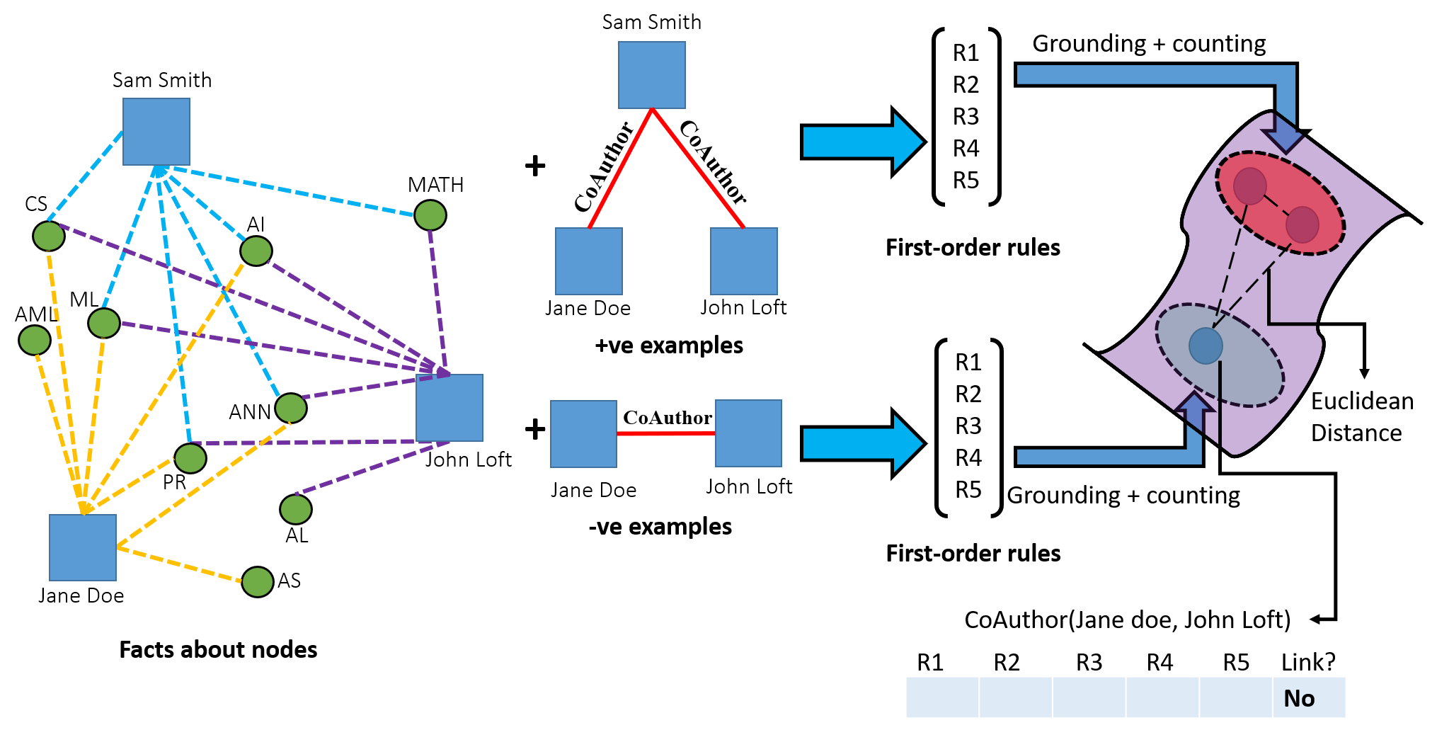
Figure 3: Learning secondary Euclidean graph (nodes) for ICML data set. Learning the +ve and -ve rules and thus features separately result in more discriminative secondary graph nodes with the +ve nodes closer to each other and distant from the -ve node.

We learn a tree-based distance iteratively to introduce new relational features that perform one-class classification. The left-most path in each relational tree is a conjunction of predicates, that is, a clause, which can be used as a relational feature. The splitting criteria is the squared error over the examples and the goal is to minimize squared error in each node. We consider only the left-most path of every tree constructed due to the fact that the right paths all involve negations. Thus a single rule is extracted from each tree. The final set of “trees” is simply a list of “first-order rules” and thus are interpretable and explainable. We now present some example first order rules learned by density estimation for 2 of our considered data sets. The first two rules for each data set are learnt for the positive examples and the next two are learnt for negative examples.

Data set: Drug-Drug Interactions

1. Rule: Interacts($d_{1}$, $d_{2}$) $\implies$ TransporterSubstrate($d_{1}$, $tr_{1}$) $\wedge$ TransporterSubstrate($d_{2}$, $tr_{1}$) $\wedge$ EnzymeInhibitor($d_{1}$, $e_{1}$) $\wedge$ EnzymeInhibitor($d_{2}$, $e_{1}$)
   

2. Rule: Interacts($d_{1}$, $d_{2}$) $\implies$ EnzymeInducer($d_{1}$, $e_{1}$) $\wedge$ EnzymeSubstrate($d_{2}$, $e_{1}$) $\wedge$ EnzymeInducer($d_{2}$, $e_{2}$) $\wedge$ EnzymeInducer($d_{1}$, $e_{2}$)
   

3. Rule: Interacts($d_{1}$, $d_{2}$) $\implies$ TargetInhibitor($d_{1}$, $t_{1}$) $\wedge$ TargetInhibitor($d_{2}$, $t_{2}$) $\wedge$ TransporterSubstrate($d_{1}$, $tr_{1}$)
   

4. Rule: Interacts($d_{1}$, $d_{2}$) $\implies$ TargetAgonist($d_{1}$, $t_{1}$) $\wedge$ TargetAgonist($d_{2}$, $t_{2}$) $\wedge$ Transpor
   terInducer($d_{1}$, $tr_{1}$) $\wedge$ TransporterInducer($d_{2}$, $tr_{2}$)
   

Data set: ICML CoAuthor

1. Rule: CoAuthor($p_{1}$, $p_{2}$) $\implies$ Affiliation($p_{1}$, $a_{1}$) $\wedge$ Affiliation($p_{2}$, $a_{1}$) $\wedge$ ResearchTopic($p_{1}$, $topic_{1}$) $\wedge$ ResearchTopic($p_{2}$, $topic_{1}$)
   

2. Rule: CoAuthor($p_{1}$, $p_{2}$) $\implies$ ResearchTopic($p_{2}$, $``Mathematical\_Optimization"$) $\wedge$ ResearchTopic($p_{1}$, $``Pattern\_Recognition"$) $\wedge$ ResearchTopic($p_{1}$,$topic_{1}$) $\wedge$
   ResearchTopic($p_{2}$,$topic_{1}$)
   

3. Rule: CoAuthor($p_{1}$, $p_{2}$) $\implies$ ResearchTopic($p_{1}$, $``Pattern\_Recognition"$) $\wedge$ Research
   Topic($p_{2}$, $``Mathematical\_Optimization"$)
   

4. Rule: CoAuthor($p_{1}$, $p_{2}$) $\implies$ Affiliation($p_{1}$, $``University\_of\_California\_Berkeley"$) $\wedge$ Affiliation($p_{2}$, $``Simons\_Institute"$)
   

Step 2: Relational Rule Matrix and Distance Matrix Construction: The learned first-order rules are then grounded to obtain all the instantiations of these rules. The counts of each feature, i.e., the count of the number of times a target example (the coauthor relation between the target entities) is satisfied in every first-order rule is obtained which forms our relational rule matrix $\mathcal{X}$. In spirit, this is similar to MLNs (Richardson and Domingos 2006) that counts the instances to obtain a marginal distribution. Instead of using the counts to compute marginals, we use them in the matrices. For example, the learned first-order rule from true instances

implies that if two persons have the same affiliation and their research interests lie in same topics, then they are likely to coauthor. Suppose the given target entities are $person_{1}$ = “Jane Doe” (JD) and $person_{2}$ = “Sam Smith”(SS). The partially grounded first-order rule can then be written as

Then substitutions for all the other entities within the first-order rule are performed and checked whether the substituted first-order rule is satisfied in the groundings. For example, the substitution ${\bm{\theta}}=\{\langle university_{1},topic_{1}\rangle/\langle UCB,Artificial\>Intelligence\rangle\}$ is satisfied but the substitution ${\bm{\theta}}=\{\langle university_{1},topic_{1}\rangle/\langle UCB,Computer\>Networks\rangle\}$ is not satisfied. Since there can be multiple values taken by $topic_{1}$ that can satisfy the first-order rule, the count of all such satisfied groundings becomes a feature value for the target query CoAuthor(Jane Doe, Sam Smith). Thus using this satisfiability count we obtain a feature set $\mathcal{X}$ of size $n\times k$ where n is number of target queries and k is number of first-order rules that represent the node features.
In order to obtain the distance matrix $\mathcal{D}$ a pairwise euclidean distance of all the node feature descriptors i.e. the counts $x_{i}\in\mathcal{X}$ is computed. Thus, every element $d_{ij}\in\mathcal{D}$,

$$d_{ij}=\|x_{i}-x_{j}\|=\sqrt{\|x_{i}\|^{2}+\|x_{j}\|^{2}-2\cdot x_{i}\cdot x_{j}}$$ (2)

Euclidean Graph GCN

The original GCN formulation (Kipf and Welling 2017) requires an adjacency matrix $\mathcal{A}$ to perform the layer-wise propagation. Instead of building the adjacency matrix from the relation triples, we use the computed geometric distance matrix $\mathcal{D}$, which is a richer structure (Rouvray and Balaban 1979; Cvetkovic et al. 1980), and use it as an approximation to the adjacency matrix for the GCN. To obtain this approximation, we perform the following steps:

[1]: A threshold, t, is set as the average of all the distances (since the distance matrix is symmetric, the average is calculated from the upper-right part).

[2]: $\forall d_{ij}\in\mathcal{D}$, new distances are computed as $\hat{d}_{ij}=d_{ij}/t$ and $\hat{d}_{ij}>$ 1 is set as 1: a far-away case.

[3]: Since the higher values in $\mathcal{D}$ represent nodes that are far as opposed to the $\mathcal{A}$ where the higher values i.e. 1 represents the nodes adjacent to each other, the distance between nodes is subtracted from 1 i.e. $\hat{d}_{ij}=1-\hat{d}_{ij}$. This is similar to $\mathcal{A}$ with $\hat{d}_{ij}$= 1 representing that two nodes are connected and $\hat{d}_{ij}$= 0 representing that two nodes are not connected with the only difference being the presence of values 0 $<\hat{d}_{ij}<$ 1 that denote the closeness of two nodes.

For a GCN with M layers, the layer wise propagation rule for the layer $l$ $\in$ M can now be written as,

$$f(H^{(l)},\mathcal{D})=\sigma(\mathcal{D}H^{(l)}W^{(l)})$$ (3)

where $H^{(0)}$ is the input layer i.e. the relational rule matrix $\mathcal{X}$ with $H^{(1)}\dots H^{(M-1)}$ being the hidden layers. Since we replace $\mathcal{A}$ with $\mathcal{D}$ before the symmetric normalization and addition of self loops, these operations are now performed on $\mathcal{D}$. The updated propagation rule is,

$$f(H^{(l)},\mathcal{D})=\sigma(\hat{\mathcal{N}}^{\frac{-1}{2}}\hat{\mathcal{D}}\hat{\mathcal{N}}^{\frac{-1}{2}}H^{(l)}W^{(l)})$$ (4)

such that $\hat{\mathcal{D}}=\mathcal{D}$ + $\mathcal{I}$ where $\mathcal{I}$ is the identity matrix and $\hat{\mathcal{N}}\in\mathbb{R}$ is the diagonal weighted node degree matrix of $\hat{\mathcal{D}}$. In summary, we learn first-order rules from separate densities independently, in the process constructing a secondary graph consisting of query variable as nodes. These learned rules are then grounded resulting in richer representation than simple node features. For obtaining distance between target triples to define adjacency, we use pairwise Euclidean distance. We present rigorous empirical evaluations next.

Table 1: Properties of data sets.

Task	Data Set	# Relations	# Facts	#+ve Examples	#-ve Examples	# Rules
Link Prediction	ICML’18	4	1395	155	6498	7
	ICLR	4	4730	990	10000	7
	DDI	14	1774	2832	3188	25

Experimental Results

We consider 3 relational data sets for link prediction(Table 1). ICML’18 consists of papers from ICML 2018, ICLR consists of papers from ICLR (2013-2019) and the prediction task is whether two people are coauthors for both data sets. Both of these data sets are extracted from the Microsoft Academic Graph (MAG) (Sinha et al. 2015). DDI is a drug-drug interaction data set (Dhami et al. 2018) and the goal is to predict whether two drugs interact. A limitation of our work is that we cannot handle multiple query variables without joint learning where one could consider every relation as the query variable in different rule learning steps to obtain embeddings w.r.t all relations and use them for the knowledge base completion tasks. We leave it as a future work.

We first learn first-order logic rules using relational density estimation (Khot, Natarajan, and Shavlik 2014) from positive examples. The number of rules learned each for positive and negative examples is shown in table 1.The relational rule matrix $\mathcal{X}$ and the distance matrix $\mathcal{D}$ are then obtained. We aim to answer the following questions:

1. Q1: How does our method perform on data sets that have few examples?

2. Q2: Is learning a secondary graph structure useful?

3. Q3: Can the combination of SRL with deep models such as GCN result in better predictive models?

4. Q4: How does rule learning from relational density estimation compare with other rule learning methods?

5. Q5: What is the effect of different distance measures on the RD²GCN performance?

6. Q6: How sensitive is RD²GCN to the choice of parameters?

Baselines

Link Prediction: We compare RD²GCN, to 12 embedding baselines in 3 categories.

1. Rule learning methods: Gaifman models (Niepert 2016): uses Gaifman locality principle (Gaifman 1982) to enumerate all hand-written first-order rules within the neighborhood of the target/query variables. After obtaining the counts for the satisfied grounded handwritten rules logistic regression is used for prediction. Neural-LP (Yang, Yang, and Cohen 2017): learns first-order rules by extending the probabilistic differentiable logic system TensorLog (Cohen 2016). metapath2vec (Dong, Chawla, and Swami 2017): generates random walks with user defined meta paths and uses a heterogeneous skip-gram model to generate embeddings. PRAGCN: makes use of relational random walks (PRA) (Lao and Cohen 2010) to learn the first-order rules (Kaur et al. 2019) and obtain the features as described in our method. The learned features are then passed on to a GCN. Node+LinkFeat (Toutanova and Chen 2015) (N+LF): is obtained by running logistic regression over the learned propositional features.

2. Relational embedding methods: ComplEx (Trouillon et al. 2016): proposes a latent factorization approach in multi-relational graphs. We use the ComplEx implementation in the AmpliGraph python library. ConvE (Dettmers et al. 2018): uses convolutions over embeddings and fully connected layers to model interactions between input entities and relationships. We use ConvE from AmpliGraph python library. SimplE (Kazemi and Poole 2018): adapts the concept of Canonical Polyadic decomposition and learns two dependent embeddings for each entity and relation to obtain a similarity score for each triple to perform link prediction. We use the tensorflow implementation.

3. GCN based methods: Relational GCN (Schlichtkrull et al. 2018): extends GCN to the relational setting. and can handle different weighted edge types i.e. relations. It uses a 2 step message passing technique to learn new node representations which are then fed to a factorization method, DistMult (Yang et al. 2015). We use the tenserflow implementation. CompGCN (Vashishth et al. 2020): jointly embeds both nodes and relations in a graph and we use PyTorch implementation.

Results

For RD²GCN, we use a GCN with 2 hidden layers each with dimension = 16 with a drop out layer between the 2 graph convolutional layers. To introduce non-linearity, we use relu between input and hidden layers and to score queries, we use $log\_softmax$ function. The examples for training, validation and testing are randomly sampled without replacement. For neural embedding baselines, since they are trained on true relations, the positive examples are randomly split to $\langle 60\%,10\%,30\%\rangle$ in training, validation and testing respectively. To obtain the different metrics for the neural embedding baseline, the scores for each pair of nodes in the test examples were thresholded by the average of the obtained scores. If the score between pair of nodes $\geq$ average score the link is predicted to be true. We run our experiments on a GPU with 8 GeForce GTX 1080 Ti cards.

Table 2: Results for Link prediction.

Data	Methods	Recall	Precision	F1	AUC-PR
ICML’18	Gaifman	0.10	0.16	0.174	0.127
	Neural-LP3	0.927	0.024	0.047	0.267
	Neural-LP10	0.891	0.035	0.069	0.143
	metapath2vec	0.836	0.209	0.335	0.286
	PRAGCN	0.0	0.0	0.0	0.512
	ComplEx	0.85	0.013	0.03	0.04
	ConvE	0.636	0.01	0.02	0.015
	SimplE	0.927	0.012	0.023	0.128
	N+LF	0.379	1.0	0.549	0.396
	R-GCN	0.636	0.07	0.13	0.13
	CompGCN	0.727	0.022	0.044	0.185
	RD2GCN	0.389	1.0	0.561	0.556
ICLR	Gaifman	0.564	0.795	0.66	0.488
	Neural-LP3	0.939	0.308	0.463	0.421
	Neural-LP10	0.987	0.275	0.429	0.453
	metapath2vec	0.828	0.338	0.480	0.641
	PRAGCN	0.0	0.0	0.0	0.544
	ComplEx	0.269	0.032	0.057	0.105
	ConvE	0.677	0.037	0.069	0.054
	SimplE	0.973	0.054	0.102	0.535
	N+LF	0.97	1.0	0.984	0.972
	R-GCN	0.667	0.783	0.720	0.763
	CompGCN	0.906	0.719	0.802	0.912
	RD2GCN	0.594	1.0	0.745	0.972
DDI	Gaifman	0.469	0.707	0.564	0.581
	Neural-LP3	0.727	0.336	0.459	0.368
	Neural-LP10	0.779	0.338	0.472	0.403
	metapath2vec	0.782	0.652	0.711	0.707
	PRAGCN	0.427	0.700	0.531	0.695
	ComplEx	0.832	0.492	0.618	0.705
	ConvE	0.931	0.384	0.544	0.678
	SimplE	0.992	0.288	0.446	0.503
	N+LF	0.682	0.924	0.785	0.781
	R-GCN	0.571	1.0	0.727	0.922
	CompGCN	0.882	0.552	0.679	0.826
	RD2GCN	0.998	0.986	0.992	0.998

(Q1. Smaller data sets) Table 2 shows the result of link prediction task. Our method outperforms all the baselines significantly in 2 of the 3 data sets with the difference being significant in the smaller data set ICML’18 and is comparable in the ICLR data set. Note that although the recall is high for the neural embedding baselines, the corresponding F1 score and AUC-PR are low which implies that the baseline relational embedding methods have a high rate of false positives. This clearly demonstrates that RD²GCN is significantly better than the strong baselines for the link prediction task. This answers Q1 affirmatively.

(Q2. Secondary graph/distance matrix impact) The main advantage of our method is learning a secondary graph structure where both link prediction and node classification tasks become simple prediction tasks in this new graph. As can be seen from the results for link prediction, a simple discriminative machine learning algorithm (logistic regression), used on top of the learned features (N+LF) performs better than the other baselines including GCN-based baselines. In case of node classification, the results are comparable.

We also compare our method with Graph Attention Networks (GATs) (Veličković et al. 2018) which uses the our learned featues with the adjacency matrix instead of a distance matrix. Figure 5 shows the results and it can be seen that using a distance matrix is also effective. This is expected since in the secondary structure, as the nodes show the query, there is no particular notion of connection between the nodes. This answers Q2 affirmatively, learning a secondary graph structure is useful for prediction tasks.

(Q3. SRL + GCN) Our results show that using SRL models (relational density estimation in our case) as the underlying feature learner which are then fed to a neural model, GCN, gives us a powerful hybrid model that can be used seamlessly with relational data. Using a SRL model as the initial layer of a neural model results in learning richer initial features set used by the neural model. This initial feature set can take advantage of underlying graph structure faithfully and thus, in accordance, leads to the neural model learning far richer abstract features which in turn leads to better predictive performance. Our evaluations on both tasks support this as our method significantly outperforms GCN baselines in all domains, answering Q3 affirmatively. Neural SRL (neuro-symbolic) models can be both interpretable and expressive.

(Q4. Effective rule learning) To answer Q4, we use 4 different rule learning methods: handwritten rules (Gaifman), NeuralLP (rule length 3 & 10), metapath2vec and PRA. Table 2 clearly demonstrate that using our density estimation method significantly outperforms all rule learning method across all domains. Comparing PRAGCN and RD²GCN is especially interesting since this shows that rule learning method plays a crucial role in learning richer features, especially in the imbalanced domains, where relational density estimation is demonstrably beneficial since both methods share the underlying GCN. The difference in performance of PRAGCN and RD²GCN is significantly high in the highly imbalanced domains ICML’18 and ICLR where the features learned by the PRA method result in all examples being classified as negative.

(Q5. Effect of distance measures) Figure 5 presents the effect of 2 other distance measures, Manhattan ($L_{1}$) and Chebyshev ($L_{\infty}$), in addition to Euclidean ($L_{2}$) on the performance of RD²GCN on the DDI data set. Since Euclidean is the straight line i.e. shortest distance between nodes, it performs the best as expected. This answers Q5.

(Q6. Effect of parameter choices) To answer Q6, we change the size of the hidden layers in the GCN as well as the number of hidden layers and test our method on ICML’18 and DDI data sets. Tables 4 and 4 show that change of these parameters have none or very minuscule effect on the overall results. This answers Q6 and also shows that the learned features by themselves are quite expressive thus removing the need for a more complex GCN.

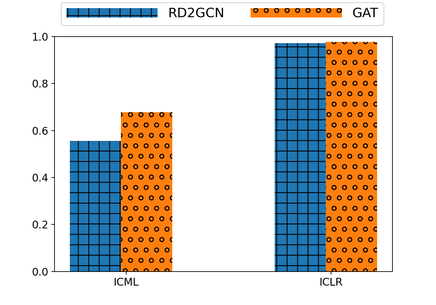
Figure 4: Comparison (AUC-PR) with GATs. DDI does not run using GAT.

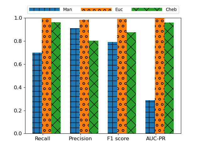
Figure 5: Effect of distance measures on the DDI data set.

Table 3: Effect of change in size of hidden layers.

Data	Size	Recall	Precision	F1 Score	AUC-PR
ICML’18	32	0.369	1.0	0.539	0.692
	64	0.369	1.0	0.539	0.692
	128	0.369	1.0	0.539	0.692
DDI	32	0.989	0.998	0.993	0.998
	64	0.989	0.998	0.993	0.998
	128	0.989	0.998	0.993	0.998

Table 4: Effect of change in # of hidden layers.

Data	#	Recall	Precision	F1 Score	AUC-PR
ICML’18	3	0.369	1.0	0.539	0.692
	4	0.369	1.0	0.539	0.692
	5	0.369	1.0	0.539	0.692
DDI	3	0.989	0.998	0.994	0.999
	4	1.0	0.997	0.998	0.999
	5	0.999	0.991	0.995	0.997

Conclusion

We presented the first GCN method that can learn from multi-relational data utilizing the different densities separately. Our method does not make assumptions on the supervision or the arity of predicates and automatically constructs rules that allow for a rich latent representation. We significantly outperform the recently successful methods on the link prediction task across multiple data sets. Allowing for joint learning and inference over multiple types of relations is an important future direction. Using more classical rule learning techniques such as (Quinlan 1990; Muggleton 1995; Srinivasan 2001) is another interesting direction. Extending our framework to node classification is the natural next step. Finally, learning in the presence of hidden/latent data and rich human domain knowledge is essential for deploying SRL methods in real tasks.

References

- Bai et al. (2019) Bai, Y.; Ding, H.; Bian, S.; Chen, T.; Sun, Y.; and Wang, W. 2019. Simgnn: A neural network approach to fast graph similarity computation. In WSDM.
- Bai et al. (2018) Bai, Y.; Ding, H.; Sun, Y.; and Wang, W. 2018. Convolutional set matching for graph similarity. NIPS.
- Balazevic, Allen, and Hospedales (2019) Balazevic, I.; Allen, C.; and Hospedales, T. 2019. Multi-relational Poincaré graph embeddings. In NIPS.
- Balažević, Allen, and Hospedales (2019a) Balažević, I.; Allen, C.; and Hospedales, T. M. 2019a. Hypernetwork knowledge graph embeddings. In ICANN.
- Balažević, Allen, and Hospedales (2019b) Balažević, I.; Allen, C.; and Hospedales, T. M. 2019b. Tucker: Tensor factorization for knowledge graph completion. EMNLP.
- Bordes et al. (2013) Bordes, A.; Usunier, N.; Garcia-Duran, A.; Weston, J.; and Yakhnenko, O. 2013. Translating embeddings for modeling multi-relational data. In NIPS.
- Cai, Zheng, and Chang (2018) Cai, H.; Zheng, V. W.; and Chang, K. C.-C. 2018. A comprehensive survey of graph embedding: Problems, techniques, and applications. TKDE.
- Cohen (2016) Cohen, W. W. 2016. Tensorlog: A differentiable deductive database. arXiv preprint arXiv:1605.06523.
- Cvetkovic et al. (1980) Cvetkovic, D. M.; Doob, M.; Sachs, H.; et al. 1980. Spectra of graphs.
- Defferrard, Bresson, and Vandergheynst (2016) Defferrard, M.; Bresson, X.; and Vandergheynst, P. 2016. Convolutional neural networks on graphs with fast localized spectral filtering. In NIPS.
- Dettmers et al. (2018) Dettmers, T.; Minervini, P.; Stenetorp, P.; and Riedel, S. 2018. Convolutional 2d knowledge graph embeddings. In AAAI.
- Dhami et al. (2018) Dhami, D. S.; Kunapuli, G.; Das, M.; Page, D.; and Natarajan, S. 2018. Drug-drug interaction discovery: kernel learning from heterogeneous similarities. Smart Health.
- Dong, Chawla, and Swami (2017) Dong, Y.; Chawla, N. V.; and Swami, A. 2017. metapath2vec: Scalable representation learning for heterogeneous networks. In KDD.
- Gaifman (1982) Gaifman, H. 1982. On local and non-local properties. In Studies in Logic and the Foundations of Mathematics.
- Getoor and Taskar (2007) Getoor, L.; and Taskar, B. 2007. Introduction to statistical relational learning. MIT press.
- He et al. (2015) He, S.; Liu, K.; Ji, G.; and Zhao, J. 2015. Learning to represent knowledge graphs with gaussian embedding. In CIKM.
- Jaeger (2007) Jaeger, M. 2007. Parameter learning for relational bayesian networks. In ICML.
- Kaur et al. (2019) Kaur, N.; Kunapuli, G.; Joshi, S.; Kersting, K.; and Natarajan, S. 2019. Neural networks for relational data. In ILP.
- Kazemi and Poole (2018) Kazemi, S. M.; and Poole, D. 2018. Simple embedding for link prediction in knowledge graphs. In NeurIPS.
- Khot, Natarajan, and Shavlik (2014) Khot, T.; Natarajan, S.; and Shavlik, J. 2014. Relational one-class classification: A non-parametric approach. In AAAI.
- Kipf and Welling (2017) Kipf, T. N.; and Welling, M. 2017. Semi-supervised classification with graph convolutional networks. ICLR.
- Kolyvakis, Kalousis, and Kiritsis (2019) Kolyvakis, P.; Kalousis, A.; and Kiritsis, D. 2019. HyperKG: Hyperbolic Knowledge Graph Embeddings for Knowledge Base Completion. arXiv preprint arXiv:1908.04895.
- Lao and Cohen (2010) Lao, N.; and Cohen, W. W. 2010. Relational retrieval using a combination of path-constrained random walks. Machine learning.
- Li et al. (2019) Li, Y.; Gu, C.; Dullien, T.; Vinyals, O.; and Kohli, P. 2019. Graph matching networks for learning the similarity of graph structured objects. ICML.
- Muggleton (1995) Muggleton, S. 1995. Inverse entailment and Progol. New generation computing.
- Natarajan et al. (2008) Natarajan, S.; Tadepalli, P.; Dietterich, T. G.; and Fern, A. 2008. Learning first-order probabilistic models with combining rules. Annals of Mathematics and Artificial Intelligence.
- Nickel, Rosasco, and Poggio (2016) Nickel, M.; Rosasco, L.; and Poggio, T. 2016. Holographic embeddings of knowledge graphs. In AAAI.
- Nickel, Tresp, and Kriegel (2011) Nickel, M.; Tresp, V.; and Kriegel, H.-P. 2011. A three-way model for collective learning on multi-relational data. In ICML.
- Niepert (2016) Niepert, M. 2016. Discriminative gaifman models. In NIPS.
- Quinlan (1990) Quinlan, J. R. 1990. Learning logical definitions from relations. Machine learning.
- Raedt et al. (2016) Raedt, L. D.; Kersting, K.; Natarajan, S.; and Poole, D. 2016. Statistical relational artificial intelligence: Logic, probability, and computation. Synthesis Lectures on Artificial Intelligence and Machine Learning.
- Richardson and Domingos (2006) Richardson, M.; and Domingos, P. 2006. Markov logic networks. Machine learning.
- Rouvray and Balaban (1979) Rouvray, D. H.; and Balaban, A. T. 1979. Chemical applications of graph theory. Applications of Graph Theory.
- Schlichtkrull et al. (2018) Schlichtkrull, M.; Kipf, T. N.; Bloem, P.; Van Den Berg, R.; Titov, I.; and Welling, M. 2018. Modeling relational data with graph convolutional networks. In European Semantic Web Conference.
- Sinha et al. (2015) Sinha, A.; Shen, Z.; Song, Y.; Ma, H.; Eide, D.; Hsu, B.-J.; and Wang, K. 2015. An overview of microsoft academic service (mas) and applications. In WWW.
- Srinivasan (2001) Srinivasan, A. 2001. The aleph manual.
- Sun et al. (2019) Sun, Z.; Deng, Z.-H.; Nie, J.-Y.; and Tang, J. 2019. Rotate: Knowledge graph embedding by relational rotation in complex space. ICLR.
- Toutanova and Chen (2015) Toutanova, K.; and Chen, D. 2015. Observed versus latent features for knowledge base and text inference. In CVSC Workshop at ACL.
- Trouillon et al. (2016) Trouillon, T.; Welbl, J.; Riedel, S.; Gaussier, É.; and Bouchard, G. 2016. Complex embeddings for simple link prediction. ICML.
- Vashishth et al. (2020) Vashishth, S.; Sanyal, S.; Nitin, V.; and Talukdar, P. 2020. Composition-based multi-relational graph convolutional networks. ICLR.
- Veličković et al. (2018) Veličković, P.; Cucurull, G.; Casanova, A.; Romero, A.; Lio, P.; and Bengio, Y. 2018. Graph attention networks. ICLR.
- Wang et al. (2017) Wang, Q.; Mao, Z.; Wang, B.; and Guo, L. 2017. Knowledge graph embedding: A survey of approaches and applications. IEEE Transactions on Knowledge and Data Engineering.
- Wang et al. (2014) Wang, Z.; Zhang, J.; Feng, J.; and Chen, Z. 2014. Knowledge graph embedding by translating on hyperplanes. In AAAI.
- Xiao, Huang, and Zhu (2016) Xiao, H.; Huang, M.; and Zhu, X. 2016. TransG: A generative model for knowledge graph embedding. In ACL.
- Yang et al. (2015) Yang, B.; Yih, W.-t.; He, X.; Gao, J.; and Deng, L. 2015. Embedding entities and relations for learning and inference in knowledge bases. ICLR.
- Yang, Yang, and Cohen (2017) Yang, F.; Yang, Z.; and Cohen, W. W. 2017. Differentiable learning of logical rules for knowledge base reasoning. In NIPS.
- Zhang et al. (2019) Zhang, S.; Tay, Y.; Yao, L.; and Liu, Q. 2019. Quaternion knowledge graph embeddings. In NIPS.