A Distance Covariance-based Estimator

Abstract

February 2020

abstract Weak instruments present a major setback to empirical work. This paper introduces an estimator that admits weak, uncorrelated, or mean-independent instruments that are non-independent of endogenous covariates. Relative to conventional instrumental variable methods, the proposed estimator weakens the relevance condition considerably without imposing a stronger exclusion restriction. Identification mainly rests on (1) a weak conditional median exclusion restriction imposed on pairwise differences in disturbances and (2) non-independence between covariates and instruments. Under mild conditions, the estimator is consistent and asymptotically normal. Monte Carlo experiments showcase an excellent performance of the estimator, and two empirical examples illustrate its practical utility.

Keywords: distance covariance, dependence, weak instrument, endogeneity, $U$-statistics
JEL classification: C13, C14, C26

February 2020

abstract Weak instruments present a major setback to empirical work. This paper introduces an estimator that admits weak, uncorrelated, or mean-independent instruments that are non-independent of endogenous covariates. Relative to conventional instrumental variable methods, the proposed estimator weakens the relevance condition considerably without imposing a stronger exclusion restriction. Identification mainly rests on (1) a weak conditional median exclusion restriction imposed on pairwise differences in disturbances and (2) non-independence between covariates and instruments. Under mild conditions, the estimator is consistent and asymptotically normal. Monte Carlo experiments showcase an excellent performance of the estimator, and two empirical examples illustrate its practical utility.

Keywords: distance covariance, dependence, weak instrument, endogeneity, $U$-statistics
JEL classification: C13, C14, C26

1 Introduction

Empirical work in economics largely depends on instrumental variable (IV) methods. When instruments are weakly correlated with endogenous covariates, these methods become unreliable; they can produce biased estimates and hypothesis tests with large size distortions. Moreover, IV methods are infeasible when instruments are uncorrelated with endogenous variables. Econometric literature on the weak instrument problem largely focusses on detection and weak-instrument-robust inference. Theoretical progress on estimation is, however, scant. This paper introduces an estimator which minimises the distance covariance (dCov) between a vector of disturbances and a set of instruments. The dCov is introduced by [60]. It measures the distributional dependence between two random variables of arbitrary dimensions. The proposed Minimum Dependence estimator (MDep hereafter) weakens the relevance (or correlatedness) requirement considerably and admits instruments that are non-independent of endogenous covariates.

The non-independence identification condition implies the MDep estimator maximises the set of relevant instruments. This feature of the proposed estimator makes it fundamentally different from conventional methods. The exclusion restriction imposed is a conditional median independence assumption on pairwise differences in disturbances. Like the uncorrelatedness exclusion restriction of standard IV methods (see, e.g., [46, Assumption 2SLS.1]), the MDep exclusion restriction is weaker than the (strong) conditional mean independence restriction (see, e.g., [9] and [14, Assumption A.1]). Unlike IV methods, however, the form of dependence between endogenous covariates and instruments needs to be neither known nor specified, effectively eliminating the sensitivity of estimates to first-stage model specification. Although the MDep estimator generally applies to linear and non-linear models typically estimated using IV methods, it shares the “robustness” feature of quantile estimators (see, e.g., [34, 29]) in the sense that its asymptotic properties do not depend on the existence of moments of the outcome variable. For example, the limit of the MDep objective function exists even if no moment of the outcome variable exists. Under mild conditions, the MDep estimator is consistent and asymptotically normal. Also, the covariance matrix estimator is shown to be consistent.

Monte Carlo simulations for the linear model demonstrate a competitive performance of the MDep estimator vis-à-vis IV and ordinary least squares (OLS) when instruments are linear in endogenous covariates. When instruments are uncorrelated or mean-independent of endogenous covariates, IV methods break down. The MDep, on the other hand, performs reasonably well. This paper considers two empirical examples that illustrate the practical usefulness of the MDep estimator. In the first example, the excluded instrument is IV-strong and hence MDep-strong by construction. Consequently, both sets of estimates and standard errors are similar. The second application presents an interesting case where the instrument has non-trivial non-linear and non-monotone identifying variation that the MDep, unlike the IV, is able to exploit. In this example, MDep estimates are more precise than the IV.

The econometric literature on weak instruments largely focusses on detection and weak-instrument-robust inference (e.g., [38, 57, 2, 52, 30, 4, 35, 3]). See [5] for an excellent review. Normal distributions of conventional IV estimates can be poor and hypothesis tests based on them can be unreliable when instruments are weak [26, 27, 8]. Although the econometric literature on weak instruments does not focus much on estimation, three exceptions deserve discussion. [18] proves that if instruments can be arbitrarily weak, no unbiased estimator exists without further restrictions. [3] shows that asymptotically unbiased estimation is possible granted one correctly imposes a sign restriction on the first-stage regression coefficient. By extracting non-linear identifying variation in instruments using machine learning techniques (e.g., neural networks and random forests) and sample splitting, [9] achieves higher precision and increased instrument strength. While it is conceivable to take transformations of the instrument to extract more variation (see, e.g., [14]), this approach may fail when the available instrument is a non-monotone function of the endogenous covariate. When it is feasible, the approach easily results in high-dimensionality (see, e.g., [6, 17]). This paper’s contribution to the literature on weak instruments is the MDep estimator. In addition to linear identifying variation in endogenous covariates that IV methods exploit, the MDep estimator exploits additional monotone and non-monotone forms of dependence that may exist between instruments and endogenous covariates for identification. The MDep gives a new perspective to handling weak IVs in empirical practice; poorly correlated, uncorrelated, or mean-independent instruments in the conventional IV setting can be MDep-strong.

Several applications of the dCov measure have emerged since the seminal paper [60]. The dCov measure is used primarily to test independence between two random variables of arbitrary dimensions. It is consistent against all types of dependent alternatives including linear, non-linear, monotone, and non-monotone forms of dependence. [59] derives the partial distance covariance ($pdCov$) test of independence between two random variables with dependence on a third set removed. Based on the dCov measure, [56] derives the martingale difference divergence (MDD) measure to test for conditional mean independence, and [32] derives a test of partial conditional mean independence. [58, 47], respectively, adapt the [56] MDD measure to test model specification in conditional mean and quantile regression models. [49] introduces the auto-covariance function for strictly stationary multivariate time series. [13] tests goodness-of-fit of time series models by applying an adapted distance covariance function to residuals. The closest work to the current paper is perhaps [37]; it proposes an estimator of single-index models as a tool for sufficient dimension reduction using the dCov as a criterion. There is a growing literature on the application of the dCov measure to variable selection and dimension reduction (see, e.g., [25, 56, 48]). The reader is referred to [15] for a review of several applications of the dCov measure. This paper is the first to introduce a dCov-based estimator of econometric models under possible endogeneity.

The rest of the paper is organised as follows. Section 2 describes the dCov measure and presents the MDep estimator. Section 3 derives important theoretical results viz. identification, consistency, asymptotic normality, and consistency of the covariance matrix estimator. Section 4 examines the finite-sample performance of the MDep estimator through simulations. Two empirical examples in Section 5 illustrate the MDep estimator’s practical utility, and Section 6 concludes. All proofs are relegated to the Appendix. Additional theoretical and simulation results are available in the Online Appendix.

2 The MDep Estimator

This section presents the MDep estimator. The estimator is based on the distance covariance measure proposed by [60].

2.1 The dCov measure

[60] introduces distance covariance (dCov) as a measure of dependence between two random variables of arbitrary dimensions. Let $\varphi_{U,Z}(t,s)$ denote the joint characteristic function of $[U,Z]$, and $[\varphi_{U}(t),\varphi_{Z}(s)]$ denote their marginal characteristic functions. The distance covariance measure is defined below.

Definition 2.1.

The distance covariance between random variables $U$ and $Z$ with finite first moments is the non-negative number $\mathcal{V}(U,Z)$ defined by

(2.1) $$\begin{split}\mathcal{V}^{2}(U,Z)&\equiv|\varphi_{U,Z}(t,s)-\varphi_{U}(t)\varphi_{Z}(s)|_{w}^{2}\\ &=\int|\varphi_{U,Z}(t,s)-\varphi_{U}(t)\varphi_{Z}(s)|^{2}w(t,s)dtds\\ &=\int\big{|}\mathbb{E}\big{[}\exp(\iota(t^{\prime}U+s^{\prime}Z))\big{]}-\mathbb{E}\big{[}\exp(\iota t^{\prime}U)\big{]}\mathbb{E}\big{[}\exp(\iota s^{\prime}Z)\big{]}\big{|}^{2}w(t,s)dtds\end{split}$$

where $\iota=\sqrt{-1}$ and the weight $w(t,s)$ is an arbitrary positive function for which the integration exists. $|\zeta|^{2}=\zeta\bar{\zeta}$, where $\bar{\zeta}$ is the complex conjugate of $\zeta$.

From (2.1), one observes that $|\varphi_{U,Z}(t,s)-\varphi_{U}(t)\varphi_{Z}(s)|_{w}^{2}\geq 0$ for all random variables $U$ and $Z$, and $|\varphi_{U,Z}(t,s)-\varphi_{U}(t)\varphi_{Z}(s)|_{w}^{2}=0$ if and only if $U$ and $Z$ are independent.

A sample from the joint distribution of $[U,X,Z]$ is denoted by the $n\times(p_{u}+p_{x}+p_{z})$ matrix $[\mathbf{U},\mathbf{X},\mathbf{Z}]$. Define $\mathbb{E}_{n}[\xi_{i}]\equiv\frac{1}{n}\sum_{i=1}^{n}\xi_{i}$ and $\mathbb{E}_{n}[\xi_{ij}]\equiv\frac{1}{n^{2}}\sum_{i=1}^{n}\sum_{j=1}^{n}\xi_{ij}$. $p_{u}=1$ is maintained throughout the rest of the paper since this paper considers only univariate response models. The distance covariance measure defined in terms of empirical characteristic functions, $|\varphi_{\mathbf{U},\mathbf{Z}}(t,s)-\varphi_{\mathbf{U}}(t)\varphi_{\mathbf{Z}}(s)|_{w,n}^{2}$, is

$$\int\big{|}\mathbb{E}_{n}\big{[}\exp(\iota tu_{i}+s^{\prime}\mathbf{z}_{i})\big{]}-\mathbb{E}_{n}\big{[}\exp(\iota tu_{i})\big{]}\mathbb{E}_{n}\big{[}\exp(\iota s^{\prime}\mathbf{z}_{i})\big{]}\big{|}^{2}w(t,s)dtds.$$

Using the weight function $w(t,s)=(c_{p_{u}}c_{p_{z}}||t||^{1+p_{u}}||s||^{1+p_{z}})^{-1}$ where $c_{p}=\frac{\pi^{(1+p)/2}}{\Gamma((1+p)/2)}$ for $p\geq 1$, $||\cdot||$ is the Euclidean norm, and $\Gamma(\cdot)$ is the complete gamma function, [60] proves the equality $|\varphi_{\mathbf{U},\mathbf{Z}}(t,s)-\varphi_{\mathbf{U}}(t)\varphi_{\mathbf{Z}}(s)|_{w,n}^{2}=\mathcal{V}_{n}^{2}(\mathbf{U},\mathbf{Z})$ where

$$\mathcal{V}_{n}^{2}(\mathbf{U},\mathbf{Z})=\mathcal{S}_{1n}(\mathbf{U},\mathbf{Z})+\mathcal{S}_{2n}(\mathbf{U},\mathbf{Z})-2\mathcal{S}_{3n}(\mathbf{U},\mathbf{Z}),$$

$\mathcal{S}_{1n}(\mathbf{U},\mathbf{Z})=\frac{1}{n^{2}}\sum_{i=1}^{n}\sum_{j=1}^{n}|u_{i}-u_{j}|\times||\mathbf{z}_{i}-\mathbf{z}_{j}||$, $\mathcal{S}_{2n}(\mathbf{U},\mathbf{Z})=\frac{1}{n^{2}}\sum_{i=1}^{n}\sum_{j=1}^{n}|u_{i}-u_{j}|\frac{1}{n^{2}}\sum_{i=1}^{n}\sum_{j=1}^{n}||\mathbf{z}_{i}-\mathbf{z}_{j}||$, and $\mathcal{S}_{3n}(\mathbf{U},\mathbf{Z})=\frac{1}{n^{3}}\sum_{i=1}^{n}\sum_{j=1}^{n}\sum_{k=1}^{n}|u_{i}-u_{j}|||\mathbf{z}_{i}-\mathbf{z}_{k}||$. The empirical distance covariance measure $\mathcal{V}_{n}^{2}(\mathbf{U},\mathbf{Z})$ simplifies to

(2.2) $$\mathcal{V}_{n}^{2}(\mathbf{U},\mathbf{Z})\equiv\frac{1}{n^{2}}\sum_{i=1}^{n}\sum_{j=1}^{n}\check{z}_{ij}\times|\tilde{u}_{ij}|$$

where $\displaystyle\check{z}_{ij}\equiv||\tilde{\mathbf{z}}_{ij}||-\frac{1}{n}\sum_{k=1}^{n}(||\tilde{\mathbf{z}}_{ik}||+||\tilde{\mathbf{z}}_{kj}||)+\frac{1}{n^{2}}\sum_{k=1}^{n}\sum_{l=1}^{n}||\tilde{\mathbf{z}}_{kl}||$, $\tilde{u}_{ij}\equiv u_{i}-u_{j}$, and $\tilde{\mathbf{z}}_{ij}\equiv\mathbf{z}_{i}-\mathbf{z}_{j}$.

[60]’s szekely2007measuring weight function $w(t,s)=(c_{p_{u}}c_{p_{z}}||t||^{1+p_{u}}||s||^{1+p_{z}})^{-1}$, besides yielding a reliable measure of dependence, results in a computationally tractable measure, obviates the choice of smoothing parameters (e.g., bandwidth or number of approximating terms in non-parametric approaches), and does not suffer from the curse of dimensionality. While the form $|\varphi_{\mathbf{U},\mathbf{Z}}(t,s)-\varphi_{\mathbf{U}}(t)\varphi_{\mathbf{Z}}(s)|_{w,n}^{2}$ of the dCov measure is natural and intuitive as a non-negative measure of distributional dependence, the form $\mathcal{V}_{n}^{2}(\mathbf{U},\mathbf{Z})$ is computationally tractable. The MDep estimator proposed in this paper is based on the latter. For the estimator presented in this paper, the simplified formulation (2.2) has two main advantages: the permutation symmetry of $\check{z}_{ij}$, i.e., $\check{z}_{ij}=\check{z}_{ji}$, simplifies the application of U-statistic theory in the proof of asymptotic normality, and lessens computational time needed to evaluate (2.2).

For ease of reference, the properties of the dCov measure in [60, 41] are stated below. The following properties of the dCov measure hold.

Properties of dCov.

1. $\displaystyle\mathcal{V}_{n}^{2}(\mathbf{U},\mathbf{Z})=|\varphi_{\mathbf{U},\mathbf{Z}}(t,s)-\varphi_{\mathbf{U}}(t)\varphi_{\mathbf{Z}}(s)|_{w,n}^{2}$.

2. $\mathcal{V}_{n}(\mathbf{U},\mathbf{Z})\geq 0$.

3. $\mathcal{V}^{2}(U,Z)=0\text{ if and only if }U$ is independent of $Z$.

4. $\displaystyle\lim_{n\rightarrow\infty}\mathcal{V}_{n}(\mathbf{U},\mathbf{Z})=\mathcal{V}(U,Z)\text{ almost surely (a.s.). }$

The properties are provided and proved in the following papers: Property (a) in [60, Theorem 1], Property (b) in [41, Theorem 4 (i)], Property (c) holds by definition (see (2.1)), and Property (d) in [60, Theorem 2]. From (2.2), it is obvious that $\mathcal{V}_{n}^{2}(\mathbf{U},\mathbf{Z})=0$ if every sample observation of $\mathbf{U}$, $\mathbf{Z}$, or both is identical. An important implication of Properties (b), (c) and (d) is that $\mathcal{V}_{n}^{2}(\mathbf{U},\mathbf{Z})=0$ if and only if $U$ is independent of $Z$ with probability approaching one (w.p.a.1).

2.2 Model specification

For considerations of space and scope, the current paper is limited to parametric regression models which assume the scalar outcome $y_{i}$ is generated by $y_{i}=G\big{(}\theta_{o,c}+g(\mathbf{x}_{i},\bm{\theta}_{o})+u_{i}\big{)}$, where $G(\cdot)$ is a known invertible function, $g(\cdot,\cdot)$ is a known differentiable function with unknown parameter vector $\bm{\theta}_{o}\in\mathbb{R}^{p_{\theta}}$, and $\theta_{o,c}$ is the intercept. By the invertibility of $G(\cdot)$, the disturbance function is $u_{i}(\bm{\theta})=G^{-1}(y_{i})-g(\mathbf{x}_{i},\bm{\theta})$. The intercept is ignored because it is differenced out in the objective function (2.3). The dependence of $u_{i}(\bm{\theta})$ on covariates $\mathbf{x}_{i}$ is suppressed for notational convenience. Observed data $[\mathbf{Y},\mathbf{X},\mathbf{Z}]$ include an $n\times 1$ vector of outcomes $\mathbf{Y}$, an $n\times p_{x}$ matrix of covariates, and an $n\times p_{z}$ matrix of instruments $\mathbf{Z}$. While the class of models under consideration includes interesting examples such as the linear model $u_{i}(\bm{\theta})=y_{i}-\mathbf{x}_{i}\bm{\theta}$, non-linear parametric models, e.g., $u_{i}(\bm{\theta})=y_{i}-\exp(\mathbf{x}_{i}\bm{\theta})$, fractional response models, e.g., $u_{i}(\bm{\theta})=\log(y_{i}/(1-y_{i}))-\mathbf{x}_{i}\bm{\theta}$, and special cases of Box-Cox models e.g., $u_{i}(\bm{\theta})=\log(y_{i})-\mathbf{x}_{i}\bm{\theta}$, it excludes equally interesting ones such as binary response models and quantile regression.

2.3 The objective function

The objective function is a squared distance covariance of $\mathbf{U}(\bm{\theta})$ and $\mathbf{Z}$, where the $i$’th element of the $n\times 1$-valued $\mathbf{U}(\bm{\theta})$ is $u_{i}(\bm{\theta})$. Using (2.2), the objective function is given by

(2.3) $$\mathcal{V}_{n}^{2}(\mathbf{U}(\bm{\theta}),\mathbf{Z})=\frac{1}{n^{2}}\sum_{i=1}^{n}\sum_{j=1}^{n}\check{z}_{ij}|\tilde{u}_{ij}(\bm{\theta})|\text{ where }\tilde{u}_{ij}(\bm{\theta})\equiv u_{i}(\bm{\theta})-u_{j}(\bm{\theta})$$

and the MDep estimator is

$$\hat{\bm{\theta}}_{n}=\operatorname*{arg\,min}_{\bm{\theta}\in\bm{\Theta}}\mathcal{V}_{n}^{2}(\mathbf{U}(\bm{\theta}),\mathbf{Z}).$$

(2.3) is a sum of specially weighted absolute pairwise differences in disturbances. (2.3) for example, explains why the asymptotic behaviour of the MDep estimator is similar to that of quantile estimators. It is instructive to note how the MDep relates to moment estimators which include conventional IV methods such as OLS, IV, 2SLS, MM, and GMM. A moment estimator typically minimises the (possibly weighted) linear dependence between $\mathbf{Z}$ and $\mathbf{U}(\bm{\theta})$ by solving $\mathbf{Z}^{\prime}\mathbf{U}(\bm{\theta})=\mathbf{0}$. The MDep, on the other hand, minimises their distributional dependence. The MDep hence minimises a more general form of dependence between $\mathbf{Z}$ and $\mathbf{U}(\bm{\theta})$.

3 Asymptotic Theory

Asymptotic theory for the MDep estimator falls within the category of estimators of models with non-smooth objective functions such as quantile regression (QR) methods, e.g., [23, 34, 29], the instrumental variable QR methods of [11, 12], the CF approach to QR of [24], and the valid moment selection procedure of [10].

Define the $n\times p_{\theta}$ matrix $\mathbf{X}^{g}(\bm{\theta})$ whose $i$’th row is $\mathbf{x}_{i}^{g}(\bm{\theta})$ where $\mathbf{x}_{i}^{g}(\bm{\theta})\equiv\frac{\partial u_{i}(\bm{\theta})}{\partial\bm{\theta}^{\prime}}$, the $n^{2}\times p_{\theta}$ matrix $\tilde{\mathbf{X}}^{g}(\bm{\theta})$ whose rows comprise $\{\tilde{\mathbf{x}}_{ij}^{g}(\bm{\theta}):1\leq i,j\leq n\}$, $\tilde{\mathbf{x}}_{ij}^{g}(\bm{\theta})\equiv\mathbf{x}_{i}^{g}(\bm{\theta})-\mathbf{x}_{j}^{g}(\bm{\theta})$, $\tilde{u}_{ij}\equiv\tilde{u}_{ij}(\bm{\theta}_{o})$, and the true parameter vector $\bm{\theta}_{o}$. Also, let $\tilde{\mathbf{x}}^{g}(\bm{\theta}),\mathbf{x}^{g}(\bm{\theta})$, $\tilde{\mathbf{z}}$, and $\check{z}$ be any random variables defined on the supports of $\tilde{\mathbf{x}}_{ij}^{g}(\bm{\theta}),\mathbf{x}_{i}^{g}(\bm{\theta})$, $\tilde{\mathbf{z}}_{ij}$, and $\check{z}_{ij}$, respectively. Define $\{\mathbf{w}_{i}:1\leq i\leq n\},\ \mathbf{w}_{i}\equiv[u_{i},\mathbf{x}_{i},\mathbf{z}_{i}]$ on a probability space $(\mathcal{W},\mathscr{W},\mathbb{P})$. Following [21], the normalised minimand is defined as $\displaystyle Q_{n}(\bm{\theta})\equiv\frac{1}{n^{2}}\sum_{i=1}^{n}\sum_{j=1}^{n}q(\mathbf{w}_{i},\mathbf{w}_{j},\bm{\theta})$, where $q(\mathbf{w}_{i},\mathbf{w}_{i},\bm{\theta})=\check{z}_{ij}\big{(}|\tilde{u}_{ij}(\bm{\theta})|-|\tilde{u}_{ij}|\big{)}$. Normalising the minimand avoids unnecessary moment conditions on $U$. See [34, 29] for example.

3.1 Regularity Conditions

Two sets of regularity conditions are imposed to guarantee the consistency of the MDep estimator $\hat{\bm{\theta}}_{n}$. The first set comprises sampling, smoothing, and dominance conditions which ensure that the difference between the normalised minimand and its expectation converges to zero uniformly in $\bm{\theta}$. These are stated below as assumptions 1(a)-1(d).

Assumption 1.

For a constant $C>0$:

1. $\mathbf{w}_{i}\equiv[u_{i},\mathbf{x}_{i},\mathbf{z}_{i}]$ are independently distributed random vectors across $i$, and the outcome is generated as $y_{i}=G\big{(}\theta_{o,c}+g(\mathbf{x}_{i},\bm{\theta}_{o})+u_{i}\big{)}$.

2. $u(\bm{\theta})$ is measurable in $[u_{i},\mathbf{x}_{i}]$ for all $\bm{\theta}$ and is twice differentiable in $\bm{\theta}$ for all $[u,\mathbf{x}]$ in the support of $[u_{i},\mathbf{x}_{i}]$. $\mathbf{x}^{g}(\bm{\theta})$ is measurable in $\mathbf{x}_{i}$ for all $\bm{\theta}$.

3. $\displaystyle\mathbb{E}\big{[}\sup_{\bm{\theta}\in\bm{\Theta}}||\max\{|\check{z}|,1\}\tilde{\mathbf{x}}^{g}(\bm{\theta})||^{4}\big{]}\leq C$.

4. $\bm{\theta}_{o}$ is in the interior of a compact subset $\bm{\Theta}$ in $\mathbb{R}^{p_{\theta}}$.

Assumptions 1 (a), (d), (c) and (b) above suffice for the application of the uniform law of large numbers in [1]. Assumption 1(a) allows for heteroskedasticity. Addressing other forms of dependence in the data, e.g., autocorrelation and clustering is beyond the scope of the current paper. The condition on the data generating process in Assumption 1(a) and the differentiability requirement in Assumption 1(b) define the class of models considered in the current paper, e.g., the linear model. They exclude models such as [23]’s koenker1978regression QR and binary response models. $\tilde{u}_{ij}(\bm{\theta})=\tilde{u}_{ij}+\tilde{\mathbf{x}}_{ij}^{g}(\bar{\bm{\theta}})(\bm{\theta}-\bm{\theta}_{o})$ for some $\bar{\bm{\theta}}$ between $\bm{\theta}$ and $\bm{\theta}_{o}$ is a useful expression for subsequent analyses thanks to Assumption 1(b) and the mean-value theorem (MVT).

Assumption 1(c) is an MDep analogue of a standard condition that uniformly bounds the fourth moment of both the weighted and unweighted Jacobian, i.e., $\displaystyle\mathbb{E}\big{[}\sup_{\bm{\theta}\in\bm{\Theta}}||\max\{|\check{z}|,1\}\tilde{\mathbf{x}}^{g}(\bm{\theta})||^{4}\big{]}\leq C$ implies both $\displaystyle\mathbb{E}\big{[}\sup_{\bm{\theta}\in\bm{\Theta}}||\check{z}\tilde{\mathbf{x}}^{g}(\bm{\theta})||^{4}\big{]}\leq C$
and $\displaystyle\mathbb{E}\big{[}\sup_{\bm{\theta}\in\bm{\Theta}}||\tilde{\mathbf{x}}^{g}(\bm{\theta})||^{4}\big{]}\leq C$. It can be shown (see Lemma A.1) that under Assumption 1(c), $\displaystyle\mathcal{B}(\mathbf{x}_{i},\mathbf{x}_{j},\mathbf{z}_{i},\mathbf{z}_{j})\equiv\sup_{\bm{\theta}\in\bm{\Theta}}||\check{z}_{ij}\tilde{\mathbf{x}}_{ij}^{g}(\bm{\theta})||$, which does not depend on $[u_{i},u_{j}]$, is integrable, and $\displaystyle|q(\mathbf{w}_{i},\mathbf{w}_{j},\bm{\theta})|\leq\mathcal{B}(\mathbf{x}_{i},\mathbf{x}_{j},\mathbf{z}_{i},\mathbf{z}_{j})||\bm{\theta}-\bm{\theta}_{o}||$ a.s. for all $\bm{\theta}_{1},\bm{\theta}_{2}\in\bm{\Theta}$. From Assumption 1(d) and the foregoing, the expected value of $q(\mathbf{w}_{i},\mathbf{w}_{j},\bm{\theta})$ exists even if the expected value of $u_{i}$ does not exist. This special feature of the MDep estimator is emphasised in the following remarks.

Remark 3.1.

Although the MDep estimator developed in this paper is not a quantile estimator, i.e., it does not estimate regression quantiles, it shares the “robustness” feature of quantile estimators over the class of models in Assumption 1(a) where the asymptotic properties do not depend on the existence of moments of the disturbance $u_{i}$.

The remaining set of regularity conditions for consistency (Assumptions 2(a) and 2(b)) are identification conditions which ensure that the expected value of the minimand is uniquely minimised at $\bm{\theta}_{o}$ in large samples.

Assumption 2.

1. Given $\tilde{\mathbf{x}}_{ij}^{g}$, the median of $\tilde{u}_{ij}$ is independent of $\check{z}_{ij}$.

2. There exists a $\tilde{\delta}_{\varepsilon}>0$ such that $\displaystyle\inf_{\{\bm{\gamma}\in\mathbb{R}^{p_{\theta}}:||\bm{\gamma}||\geq\varepsilon\}}\mathbb{E}[\mathcal{V}_{n}^{2}(\mathbf{X}^{g}(\bm{\theta})\bm{\gamma},\mathbf{Z})]>\tilde{\delta}_{\varepsilon}$ for any $\varepsilon>0$, $\bm{\theta}\in\bm{\Theta}$, and $n$ sufficiently large.

These assumptions are perhaps the most important because one easily sees the advantage the MDep estimator has vis-à-vis conventional IV methods. While the exclusion restriction (Assumption 2(a)), like that of conventional methods, is not stronger than the conditional mean independence exclusion restriction, the relevance condition (Assumption 2(b)) is much weaker.

Assumption 2(a) requires that the median of $\tilde{u}_{ij}$ conditional on $[\mathbf{x}_{ij}^{g},\check{z}_{ij}]$ be constant. Unlike Assumption 2(a) which is imposed on the pairwise differences in disturbances, similar exclusion restrictions on conditional quantiles are imposed on the levels of disturbances for quantile estimators under (possible) endogeneity (see, e.g., [11, Assumption A.2], [24, Assumption 3.6], and [34, Assumption B2]). Specific to the median of $u_{i}$, [24], for example, requires that the median of $u_{i}$, conditional on $[\mathbf{x}_{i},\mathbf{z}_{i}]$ be constant. By the symmetry of the unconditional density of $\tilde{u}_{ij}$ around zero, Assumption 2(a) is equivalent to a conditional mean independence restriction $\mathbb{E}[\tilde{u}_{ij}|\tilde{\mathbf{x}}_{ij}^{g},\check{z}_{ij}]=\mathbb{E}[\tilde{u}_{ij}|\tilde{\mathbf{x}}_{ij}^{g}]$ if the expected value of $u_{i}$ exists. In words, $\mathbb{E}[\tilde{u}_{ij}|\tilde{\mathbf{x}}_{ij}^{g},\check{z}_{ij}]=\mathbb{E}[\tilde{u}_{ij}|\tilde{\mathbf{x}}_{ij}^{g}]$ says given $\tilde{\mathbf{x}}_{ij}^{g}$, the mean of $\tilde{u}_{ij}$ is independent of $\check{z}_{ij}$. Assumption 2(a) is implied by the stronger conditional mean-independence condition $\mathbb{E}[u_{i}|\tilde{\mathbf{x}}_{ij}^{g},\check{z}_{ij}]=\mathbb{E}[u_{i}|\tilde{\mathbf{x}}_{ij}^{g}]$. Taking the expectation of both sides conditional on $\mathbf{w}_{i}$ gives the more familiar conditional mean-independence exclusion restriction in levels $\mathbb{E}[u_{i}|\mathbf{x}_{i}^{g},\mathbf{z}_{i}]=\mathbb{E}[u_{i}|\mathbf{x}_{i}^{g}]$. This sufficient (but not necessary) condition for Assumption 2(a) can be verified using the conditional mean independence specification test of [58]. Both the MDep exclusion restriction Assumption 2(a) and the uncorrelatedness exclusion restriction of conditional IV methods (see, e.g., [46, Assumption 2SLS.1]) are weaker than the conditional mean-independence condition. Simulations in Section 4 suggest the MDep exclusion restriction (Assumption 2(a)) is not stronger than the uncorrelatedness exclusion restriction of conventional IV methods.

Assumption 2(b) is the condition of non-independence between $X$ and $Z$; it is the MDep analogue of the relevance condition in the IV/CF setting (see, e.g., [46, asummption 2SLS.2(b)]). Like the IV relevance condition, Assumption 2(b) ensures that dependence between each endogenous covariate and its excluded instrument holds after netting out dependence on all other covariates. This suggests that the partial distance covariance $pdCov$ test of [59] can be used to test Assumption 2(b) when there is a single endogenous covariate. Assumption 2(b) is, however, a significantly weaker assumption. For example, suppose there is one endogenous covariate $X$ and a single instrument $Z$. A standard IV relevance condition is that $X$ be correlated with $Z$. The MDep, on the other hand simply requires that $X$ be non-independent of $Z$. This effectively allows $X$ to be uncorrelated, or even mean-independent of $Z$ as long as some points on its distribution are not independent of $Z$. All strong instruments in the conventional IV sense are MDep-strong. The converse is, however, not true. This idea is further explored in Section 4 via simulations. Assumption 2(b) fails when the Jacobian matrix $\mathbf{X}^{g}(\cdot)$ does not have full column rank or when instruments are fewer than parameters, i.e., $p_{z}<p_{\theta}$. To see this, note that $\mathbf{X}^{g}(\cdot)\bm{\gamma}$ can be zero (which implies $\mathcal{V}_{n}^{2}(\mathbf{X}^{g}(\cdot)\bm{\gamma},\mathbf{Z})=0$ w.p.a.1) for $\bm{\gamma}\not=\mathbf{0}$ if $\mathbf{X}^{g}(\cdot)$ does not have full column rank. Also, if instruments are fewer than parameters, it is easy to construct an example where $\mathcal{V}_{n}^{2}(\mathbf{X}^{g}(\cdot)\bm{\gamma},\mathbf{Z})=0$ w.p.a.1 for $\mathbf{X}$ not independent of $\mathbf{Z}$ and $\bm{\gamma}\not=\mathbf{0}$.

Remark 3.2.

MDep admits the largest set of instruments possible. In addition to IV-relevant instruments that both MDep and conventional IV methods admit, MDep admits instruments that are uncorrelated or mean-independent but non-independent of covariates. This clear advantage of the MDep over IV methods does not come at an added cost as the MDep exclusion restriction (Assumption 2(a)), like the uncorrelatedness exclusion restriction of IV methods, is weaker than the conditional mean independence restriction.

3.2 Consistency

The support of $\check{z}_{ij}$ is not non-negative. This makes identification proof techniques based on convexity of the objective function (see, e.g., [23, 34, 29]) inapplicable to the MDep. The non-negativity of the dCov measure (Property (b)) is, instead, exploited to establish identification. Define a set-valued map indexed by $\bm{\theta}\in\bm{\Theta}$, $\mathscr{A}_{\theta}:[0,1]\twoheadrightarrow\mathcal{W}$ where $\mathscr{A}_{\theta}(\tau)=\{\mathbf{x},\mathbf{x}^{\dagger},\mathbf{z},\mathbf{z}^{\dagger}\in\mathcal{W}:F_{\tilde{U}|\tilde{X}^{g},\hat{Z}}(\lambda_{u}\tilde{\mathbf{x}}^{g}(\bar{\bm{\theta}})(\bm{\theta}-\bm{\theta}_{o}))=\tau\}$, $[\mathbf{x}^{\dagger},\mathbf{z}^{\dagger}]$ is an independent copy of $[\mathbf{x},\mathbf{z}]$, $\lambda_{u}\in(0,1)$, and $\bar{\bm{\theta}}$ satisfies $\tilde{u}(\bm{\theta})=\tilde{u}+\tilde{\mathbf{x}}^{g}(\bar{\bm{\theta}})(\bm{\theta}-\bm{\theta}_{o})$. The following provides an important result for identification.

Proposition 3.1.

Suppose Assumptions 1(b) and 2(a) hold, then for any $\mathbf{w},\mathbf{w}^{\dagger}$ defined on the support of $\mathbf{w}_{i}$,

$$\mathbb{E}[q(\mathbf{w},\mathbf{w}^{\dagger},\bm{\theta})]=\int_{0}^{1}|2\tau-1|\int_{\mathscr{A}_{\theta}(\tau)}\big{[}\check{z}\big{|}\tilde{\mathbf{x}}^{g}(\bar{\bm{\theta}})(\bm{\theta}-\bm{\theta}_{o})\big{|}\big{]}d\mathbb{P}_{\tilde{X}^{g},\hat{Z}}d\tau.$$

The inner integrand $\check{z}\big{|}\tilde{\mathbf{x}}^{g}(\bar{\bm{\theta}})(\bm{\theta}-\bm{\theta}_{o})\big{|}$ has the same form as the summands of (2.2). This is important because the expectation of the normalised minimand can be expressed in terms of the distance covariance between $\mathbf{X}^{g}(\bar{\bm{\theta}})(\bm{\theta}-\bm{\theta}_{o})$ and $\mathbf{Z}$ for all $\bm{\theta}\not=\bm{\theta}_{o}$ and $\bar{\bm{\theta}}$ between $\bm{\theta}$ and $\bm{\theta}_{o}$. Identification then follows from Assumption 2(b).

Lemma 3.1.

Suppose Assumptions 1(b) and 2 hold, then for any $\varepsilon>0$ and $n$ sufficiently large, there exists a $\delta_{\varepsilon}>0$ such that $\displaystyle\inf_{\{\bm{\theta}\in\bm{\Theta}:||\bm{\theta}-\bm{\theta}_{o}||\geq\varepsilon\}}\mathbb{E}[Q_{n}(\bm{\theta})]>\delta_{\varepsilon}$.

Consistency of the MDep estimator is presented in the following theorem.

Theorem 1 (Consistency).

Under Assumptions 1 and 2, $\hat{\bm{\theta}}_{n}\overset{p}{\rightarrow}\bm{\theta}_{o}$.

3.3 Asymptotic normality

Notice that $\check{z}_{ij}$ is not a bona fide function of $[\mathbf{z}_{i},\mathbf{z}_{j}]$ because it is dependent on other observations. To simplify the study of the asymptotic distribution of the MDep estimator, the asymptotically equivalent function, $\displaystyle\hat{z}_{ij}=\mathcal{D}_{n}(\mathbf{z}_{i},\mathbf{z}_{j})\equiv||\mathbf{z}_{i}-\mathbf{z}_{j}||-\frac{1}{n}\sum_{k=1}^{n}\big{(}\mathbb{E}[(||\mathbf{z}_{i}-\mathbf{z}_{k}||)|\mathbf{z}_{i}]+\mathbb{E}[(||\mathbf{z}_{k}-\mathbf{z}_{j}||)|\mathbf{z}_{j}]\big{)}+\frac{1}{n^{2}}\sum_{k=1}^{n}\sum_{l=1}^{n}\mathbb{E}[||\mathbf{z}_{k}-\mathbf{z}_{l}||]$, is used instead of $\check{z}_{ij}$. Denote the equivalent normalised minimand by $\mathcal{Q}_{n}(\bm{\theta})\equiv\frac{1}{n^{2}}\sum_{i=1}^{n}\sum_{j=1}^{n}\hat{z}_{ij}\big{(}|\tilde{u}_{ij}(\bm{\theta})|-|\tilde{u}_{ij}|\big{)}$. It is shown in Lemma D.1 that the normalised minimands $Q_{n}(\bm{\theta})$ and $\mathcal{Q}_{n}(\bm{\theta})$ are asymptotically equivalent for all $\bm{\theta}\in\bm{\Theta}$. Using the form $\mathcal{Q}_{n}(\bm{\theta})$ not only simplifies the application of [19]’s hoeffding_1948 U-statistic theory for the proof of asymptotic normality but also leads to a less cumbersome and a computationally less expensive covariance matrix of the score (see Lemma D.3).

Define $\bm{\psi}(\mathbf{w}_{i},\mathbf{w}_{j})\equiv\hat{z}_{ij}\big{(}1-2\mathrm{I}(\tilde{u}_{ij}<0)\big{)}\tilde{\mathbf{x}}_{ij}^{g}(\bm{\theta}_{o})^{\prime}$. $\hat{z}_{ij}=\hat{z}_{ji}$ and $\big{(}1-2\mathrm{I}(\tilde{u}_{ij}<0)\big{)}\tilde{\mathbf{x}}_{ij}^{g}(\bm{\theta}_{o})=\big{(}1-2\mathrm{I}(\tilde{u}_{ji}<0)\big{)}\tilde{\mathbf{x}}_{ji}^{g}(\bm{\theta}_{o})$ hence $\bm{\psi}(\cdot,\cdot)$ is permutation symmetric. The score function at $\bm{\theta}_{o}$ is $\mathcal{S}_{n}(\bm{\theta}_{o})\equiv\frac{\partial\mathcal{Q}_{n}(\bm{\theta})}{\partial\bm{\theta}^{\prime}}\big{|}_{\bm{\theta}=\bm{\theta}_{o}}=\frac{1}{n^{2}}\sum_{i=1}^{n}\sum_{j=1}^{n}\bm{\psi}(\mathbf{w}_{i},\mathbf{w}_{j})^{\prime}$. By the permutation symmetry of $\bm{\psi}(\cdot,\cdot)$ and for any $\bm{\uptau}_{n}\in\mathbb{R}^{p_{\theta}}$ such that $||\bm{\uptau}_{n}||=1$, let $\mathsf{V}_{n}=\bm{\uptau}_{n}^{\prime}\mathcal{S}_{n}(\bm{\theta}_{o})^{\prime}=\frac{1}{n^{2}}\sum_{i=1}^{n}\sum_{j=1}^{n}\bm{\uptau}_{n}^{\prime}\bm{\psi}(\mathbf{w}_{i},\mathbf{w}_{j})=(1-1/n)\mathsf{U}_{n}$, where
$\mathsf{U}_{n}=\binom{n}{2}^{-1}\sum_{i=1}^{n}\sum_{j=1}^{n}\frac{1}{2}\bm{\uptau}_{n}^{\prime}\bm{\psi}(\mathbf{w}_{i},\mathbf{w}_{j})$. $\mathbb{E}[\bm{\psi}(\mathbf{w}_{i},\mathbf{w}_{j})]=\mathbf{0}$ for $1\leq i,j\leq n$ (see Lemma D.3) implies $\mathbb{E}[\mathsf{U}_{n}]=0$. $\mathsf{U}_{n}$ is a $U$-statistic (see, e.g., [19] and [45, chapter 11]). The connection to U-statistics is particularly useful for establishing a central limit theorem on $\sqrt{n}\mathcal{S}_{n}(\bm{\theta})$ because $\{\bm{\psi}(\mathbf{w}_{i},\mathbf{w}_{j}),1\leq i,j\leq n\}$ are dependent and standard central limit theorems do not apply directly. Under Assumption 1(a), the Hajék projection of $\mathsf{U}_{n}$ is $\hat{\mathsf{U}}_{n}\equiv\sum_{i=1}^{n}\mathbb{E}[\mathsf{U}_{n}|\mathbf{w}_{i}]=\frac{1}{n}\sum_{i=1}^{n}\bm{\uptau}_{n}^{\prime}\bm{\psi}_{i}(\mathbf{w}_{i})$ where $\bm{\psi}_{i}(\mathbf{w}_{i})\equiv\frac{1}{n-1}\sum_{j\not=i}\mathbb{E}[\bm{\psi}(\mathbf{w}_{i},\mathbf{w}_{j})|\mathbf{w}_{i}]$ (see, e.g., [19, eqn. 8.1] and [45, Lemma 11.10]). $\{\bm{\psi}_{i}(\mathbf{w}_{i}),1\leq i\leq n\}$ are independently distributed random vectors, and the Lyapunov central limit theorem (CLT) applies. Denote $\bm{\Psi}_{n}\equiv\mathrm{var}(\sqrt{n}\hat{\mathsf{U}}_{n})=\mathrm{var}(\frac{1}{\sqrt{n}}\sum_{i=1}^{n}\bm{\psi}_{i}(\mathbf{w}_{i}))=\frac{1}{n}\sum_{i=1}^{n}\mathbb{E}[\bm{\psi}_{i}(\mathbf{w}_{i})\bm{\psi}_{i}(\mathbf{w}_{i})^{\prime}]$.

Define $\vartheta_{n}(\bm{\theta})=\mathcal{Q}_{n}(\bm{\theta})-\mathcal{S}_{n}(\bm{\theta}_{o})(\bm{\theta}-\bm{\theta}_{o})$, then by Lemma D.3, $\mathbb{E}[\vartheta_{n}(\bm{\theta})]=\mathbb{E}[\mathcal{Q}_{n}(\bm{\theta})]-\mathbb{E}[\mathcal{S}_{n}(\bm{\theta}_{o})](\bm{\theta}-\bm{\theta}_{o})=\mathbb{E}[\mathcal{Q}_{n}(\bm{\theta})]$. $\mathcal{R}_{n}(\bm{\theta})=\sqrt{n}(\vartheta_{n}(\bm{\theta})-\mathbb{E}[\vartheta_{n}(\bm{\theta})])/||\bm{\theta}-\bm{\theta}_{o}||$ is the remainder term of the Taylor approximation (see, e.g., [33, 28, sect. 7]). Define $\bm{\Sigma}_{o}\equiv\bm{H}_{o}^{-1}\bm{\Omega}_{o}\bm{H}_{o}^{-1}$ where $\displaystyle\bm{\Omega}_{o}\equiv\lim_{n\rightarrow\infty}\mathbb{E}[\bm{\Omega}_{n}(\bm{\theta}_{o})]$, $\mathrm{var}(\sqrt{n}\mathcal{S}_{n}(\bm{\theta}_{o}))=\mathbb{E}[\bm{\Omega}_{n}(\bm{\theta}_{o})]$, $\displaystyle\bm{H}_{o}\equiv\lim_{n\rightarrow\infty}\mathbb{E}[\bm{H}_{n}(\bm{\theta}_{o})]$, and $\displaystyle\mathbb{E}[\bm{H}_{n}(\bm{\theta}_{o})]=\frac{\partial\mathbb{E}[\mathcal{S}_{n}(\bm{\theta})]}{\partial\bm{\theta}}\Big{|}_{\bm{\theta}=\bm{\theta}_{o}}$, the Hessian matrix (see Lemmata Lemmas D.3 and D.4). The expressions for $\mathbb{E}[\bm{\Omega}_{n}(\bm{\theta}_{o})]$ and $\mathbb{E}[\bm{H}_{n}(\bm{\theta}_{o})]$ are

(3.1) $$\begin{split}\mathbb{E}[\bm{\Omega}_{n}(\bm{\theta}_{o})]&=\frac{1}{n^{3}}\sum_{i=1}^{n}\sum_{j=1}^{n}\sum_{k\not=i,j}^{n}\mathbb{E}\Big{[}\hat{z}_{ij}^{2}\tilde{\mathbf{x}}_{ij}^{g}(\bm{\theta}_{o})^{\prime}\tilde{\mathbf{x}}_{ij}^{g}(\bm{\theta}_{o})\\ &+8\hat{z}_{ij}\hat{z}_{ik}\mathrm{cov}\big{(}\mathrm{I}(\tilde{u}_{ij}<0),\mathrm{I}(\tilde{u}_{ik}<0)|\bm{\omega}_{ijk}^{\tilde{x},\hat{z}}\big{)}\tilde{\mathbf{x}}_{ij}^{g}(\bm{\theta}_{o})^{\prime}\tilde{\mathbf{x}}_{ik}^{g}(\bm{\theta}_{o})\Big{]}\end{split}$$

and

(3.2) $$\mathbb{E}[\bm{H}_{n}(\bm{\theta}_{o})]=\frac{2}{n^{2}}\sum_{i=1}^{n}\sum_{j=1}^{n}\mathbb{E}\Big{[}\hat{z}_{ij}f_{\tilde{U}|\tilde{X}^{g},\hat{Z}}(0|\bm{\omega}_{ij}^{\tilde{x},\hat{z}})\tilde{\mathbf{x}}_{ij}^{g}(\bm{\theta}_{o})^{\prime}\tilde{\mathbf{x}}_{ij}^{g}(\bm{\theta}_{o})\Big{]}$$

where $\bm{\omega}_{ijk}^{\tilde{x},\hat{z}}\equiv\sigma(\mathbf{x}_{i},\mathbf{x}_{j},\mathbf{x}_{k},\mathbf{z}_{i},\mathbf{z}_{j},\mathbf{z}_{k})$, $\bm{\omega}_{ij}^{\tilde{x},\hat{z}}\equiv\sigma(\mathbf{x}_{i},\mathbf{x}_{j},\mathbf{z}_{i},\mathbf{z}_{j})$, $\sigma(\cdot)$ denotes the sigma algebra generated by its argument, and $\mathrm{cov}(\xi_{a},\xi_{b}|\xi_{c})$ denotes covariance of $\xi_{a}$ and $\xi_{b}$ conditional on $\xi_{c}$. Let $\rho_{min}(\mathbf{A})$ denote the minimum eigen-value of $\mathbf{A}$. The following additional assumptions are needed to establish the asymptotic distribution of the MDep estimator.

Assumption 3.

For the constant $C$ defined in Assumption 1:

1. $\rho_{min}(\bm{\Psi}_{n})>C^{1/2}/4$ for all $n$ sufficiently large.

2. $\displaystyle\sup_{||\bm{\theta}-\bm{\theta}_{o}||\leq\delta_{n}}\frac{|\mathcal{R}_{n}(\bm{\theta})|}{1+\sqrt{n}||\bm{\theta}-\bm{\theta}_{o}||}\overset{p}{\rightarrow}0$ for any $\delta_{n}\rightarrow 0$.

3. $\bm{H}_{o}$ is non-singular.

4. The conditional distribution of $\tilde{u}$, $F_{\tilde{U}|\tilde{X}^{g},\hat{Z}}(\cdot)$, is differentiable with density $f_{\tilde{U}|\tilde{X}^{g},\hat{Z}}(\cdot)$, $\displaystyle C^{-1}<f_{\tilde{U}|\tilde{X}^{g},\hat{Z}}(\epsilon)\leq\sup_{\gamma\in\mathbb{R}}f_{\tilde{U}|\tilde{X}^{g},\hat{Z}}(\gamma)\leq C^{1/4}$, and $|f_{\tilde{U}|\tilde{X}^{g},\hat{Z}}(\epsilon_{1})-f_{\tilde{U}|\tilde{X}^{g},\hat{Z}}(\epsilon_{2})|\leq C^{1/4}|\epsilon_{1}-\epsilon_{2}|$ a.s. for all $\epsilon,\epsilon_{1},\epsilon_{2}$ in a neighbourhood of zero and $\tilde{u}$ defined on the support of $\tilde{u}_{ij}$.

5. $\displaystyle\mathbb{E}\big{[}\sup_{\bm{\theta}\in\bm{\Theta}}||\max\{|\hat{z}|,1\}\tilde{\mathbf{x}}^{g}(\bm{\theta})||^{4}\big{]}\leq C$, $\displaystyle\mathbb{E}\big{[}\sup_{\bm{\theta}\in\bm{\Theta}}\big{|}\big{|}\hat{z}\frac{\partial\tilde{\mathbf{x}}^{g}(\bm{\theta})}{\partial\bm{\theta}}\big{|}\big{|}^{4}\big{]}\leq C$, and $\mathbb{E}\big{[}||\tilde{\mathbf{z}}||^{4}\big{]}\leq C$.

Assumption 3(a) means $\bm{\Psi}_{n}$ is positive definite. A necessary (but not sufficient) condition for this is the full column rank condition of the Jacobian matrix $\mathbf{X}^{g}(\cdot)$. Assumption 3(b) is is a stochastic equi-continuity condition for establishing the asymptotic normality of estimators with non-smooth objective functions (see, e.g., [33, 31, 10]). It is verified in Lemma D.6. Non-singularity of the Hessian (Assumption 3(c)) is imposed instead of positive definiteness because the MDep objective function (2.3) is not convex. Assumption 3(d) is a standard assumption for quantile estimators (see, e.g., [24, Assumption 3.6], [11, Assumption 2 R.4], [12, Assumption R.4], [34, Assumption C4. (i) and (ii)], and [29, Assumption A.14]); it ensures the Hessian is well-defined. The first statement in Assumption 3(e) simply adapts Assumption 1(c) for the equivalent normalised minimand $\mathcal{Q}_{n}(\bm{\theta})$. The second statement is required to apply the dominated convergence theorem in the derivation of the Hessian (see Lemmata D.4 and D.5). The third statement is an MDep analogue of a standard regularity condition (e.g., [10, condition 4.1 (iii)]); it is used in Lemma D.1(a) to show that $|\check{z}_{ij}-\hat{z}_{ij}|=O_{p}(n^{-1/2})$ for $1\leq i,j\leq n$. The asymptotic normality of the MDep estimator is stated below.

Theorem 2.

Suppose Assumptions 1, 2 and 3 hold, then

1. $\sqrt{n}\tilde{\bm{\uptau}}_{n}^{\prime}\mathbb{E}[\bm{\Omega}_{n}(\bm{\theta}_{o})]^{-1/2}\mathcal{S}_{n}(\bm{\theta}_{o})^{\prime}\overset{d}{\rightarrow}\mathcal{N}(0,1)$ for any $\tilde{\bm{\uptau}}_{n}\in\mathbb{R}^{p_{\theta}}$ with $||\tilde{\bm{\uptau}}_{n}||=1$;

2. $\sqrt{n}(\hat{\bm{\theta}}_{n}-\bm{\theta}_{o})\overset{d}{\rightarrow}\mathcal{N}(\mathbf{0},\bm{\Sigma}_{o})$.

Theorem 2(a) together with the Cramér-Wold device yields the asymptotic normality of $\sqrt{n}\mathcal{S}_{n}(\bm{\theta}_{o})$, i.e, $\sqrt{n}\mathcal{S}_{n}(\bm{\theta}_{o})\overset{d}{\rightarrow}\mathcal{N}(\mathbf{0},\bm{\Omega}_{o})$. This result plays a crucial role in the proof of Theorem 2(b) (see, e.g., [28, Theorem 7.1]).

3.4 Consistent covariance matrix estimation

The preceding subsection presents the asymptotic normality of the MDep estimator. This subsection provides the covariance matrix estimator and proves its consistency. Consistency of the covariance estimator is essential for statistical inference procedures viz. Wald tests, and confidence intervals. The approach adopted follows [34]. The estimators of $\bm{\Omega}_{o}$ and $\bm{H}_{o}$ are given by

$$\begin{split}\check{\bm{\Omega}}_{n}(\hat{\bm{\theta}}_{n})&=\frac{1}{n^{3}}\sum_{i=1}^{n}\sum_{j=1}^{n}\sum_{k\not=i,j}^{n}\Big{\{}\check{z}_{ij}^{2}\tilde{\mathbf{x}}_{ij}^{g}(\hat{\bm{\theta}}_{n})^{\prime}\tilde{\mathbf{x}}_{ij}^{g}(\hat{\bm{\theta}}_{n})\\ &+2\check{z}_{ij}\check{z}_{ik}\big{(}4\big{(}\mathrm{I}(\tilde{u}_{ij}(\hat{\bm{\theta}}_{n})<0)\mathrm{I}(\tilde{u}_{ik}(\hat{\bm{\theta}}_{n})<0)\big{)}-1\big{)}\tilde{\mathbf{x}}_{ij}^{g}(\hat{\bm{\theta}}_{n})^{\prime}\tilde{\mathbf{x}}_{ik}^{g}(\hat{\bm{\theta}}_{n})\Big{\}}\\ &\text{ and }\\ \check{\bm{H}}_{n}(\hat{\bm{\theta}}_{n})&=\frac{1}{n^{2}\hat{c}_{n}}\sum_{i=1}^{n}\sum_{j=1}^{n}\Big{\{}\mathrm{I}(|\tilde{u}_{ij}(\hat{\bm{\theta}}_{n})|\leq\hat{c}_{n})\check{z}_{ij}\tilde{\mathbf{x}}_{ij}^{g}(\hat{\bm{\theta}}_{n})^{\prime}\tilde{\mathbf{x}}_{ij}^{g}(\hat{\bm{\theta}}_{n})\Big{\}}\end{split}$$

respectively where $\hat{c}_{n}$ is a (possibly random) bandwidth and the uniform kernel replaces the conditional density in $\mathbb{E}[\bm{H}_{n}(\bm{\theta}_{o})]$. The estimator of the covariance matrix is $\bm{\Sigma}_{n}(\bm{\hat{\bm{\theta}}}_{n})=\check{\bm{H}}_{n}(\hat{\bm{\theta}}_{n})^{-1}\check{\bm{\Omega}}_{n}(\hat{\bm{\theta}}_{n})\check{\bm{H}}_{n}(\hat{\bm{\theta}}_{n})^{-1}$. In addition to preceding assumptions, the following condition is imposed on the sequence of bandwidths $\hat{c}_{n}$.

Assumption 4.

For some non-stochastic sequence $c_{n}$ with $c_{n}\rightarrow 0$ and $\sqrt{n}c_{n}\rightarrow\infty$, $\displaystyle\operatorname*{plim}_{n\rightarrow\infty}(\hat{c}_{n}/c_{n})=1$.

Assumption 4 is [34]’s powell1991estimation Assumption D1 for proving the consistency of $\check{\bm{H}}_{n}(\hat{\bm{\theta}}_{n})$; it means $\hat{c}_{n}$ satisfies $\hat{c}_{n}=o_{p}(1)$ and $\hat{c}_{n}^{-1}=o_{p}(\sqrt{n})$. The next theorem states the consistency of $\bm{\Sigma}_{n}(\bm{\hat{\bm{\theta}}}_{n})$.

Theorem 3.

Under Assumptions 1, 2, 3 and 4, $\displaystyle\operatorname*{plim}_{n\rightarrow\infty}\bm{\Sigma}_{n}(\bm{\hat{\bm{\theta}}}_{n})=\bm{\Sigma}_{o}$.

Estimating the asymptotic covariance matrix involves specifying the bandwidth $\hat{c}_{n}$. Poor performance of the covariance matrix can result from an inappropriate choice of bandwidth. In addition to the asymptotic covariance matrix estimator $\bm{\Sigma}_{n}(\bm{\hat{\bm{\theta}}}_{n})$, this paper considers the bootstrap. The bootstrap obviates the specification of $\hat{c}_{n}$. Simulations on the coverage performance of the estimator $\bm{\Sigma}_{n}(\bm{\hat{\bm{\theta}}}_{n})$ and the bootstrap are available in the Online Appendix.

4 Monte Carlo Simulations

This section examines the empirical performance of the MDep estimator vis-à-vis IV methods for the linear model using simulations. Non-linear parametric models are considered in the Online Appendix where the MDep is compared to maximum likelihood, quasi-maximum likelihood, GMM, and the control function (CF) approach.

Each element of $\mathbf{x}=[x_{1},x^{*}]$ is standard normal $\mathcal{N}(0,1)$ with $\mathrm{cov}(x_{1},x^{*})=0.25$, and $\mathbf{z}=[z_{1},z_{2}]$ are the instruments. $\theta_{c}=0.4$ and $\bm{\theta}\equiv[\theta_{1},\theta_{2}]=[1,-1]$ are maintained across all specifications. For each specification, the mean bias (MB), median absolute deviation (MAD), and root mean squared error (RMSE) are reported. $2000$ simulations are run for each sample size $n\in\{100,500,2500\}$. $\nu\sim(\chi^{2}(1)-1)/\sqrt{2}$, $\sigma_{\xi}$ is the standard deviation of a random variable $\xi$, $\mathrm{Ber}(0.5)$ is the Bernouilli distribution with mean equal to $0.5$, $\phi(\cdot)$ is the standard normal probability density function (pdf), $\Phi^{-1}(\uptau)$ is the $\uptau$’th quantile of the standard normal distribution, and $M_{\mathbf{x}}(\xi)$ is the residual from the linear projection of $\xi$ on $\mathbf{x}$. The following specifications are considered.

1. $y=\theta_{c}+\theta_{1}x_{1}+\theta_{2}x_{2}+u$, $u=(\dot{u}-\mathbb{E}[\dot{u}])/\sigma_{\dot{u}}$, $\dot{u}=\nu+\phi((x_{1}-x^{*})/0.97)$, $x_{2}=x^{*}$, and $\mathbf{z}=[x_{1},x^{*}]$.

2. $y=\theta_{c}+\theta_{1}x_{1}+\theta_{2}x_{2}+u$, $u=(\dot{u}-\mathbb{E}[\dot{u}])/\sigma_{\dot{u}}$, $\dot{u}=\nu+\phi((x_{1}-x^{*})/0.97)$, $x_{2}=(x^{*}+\nu)/\sqrt{2}$, $\mathbf{z}=[x_{1},(x^{*}+w)/\sqrt{2}]$, and $w\sim\mathcal{N}(0,1)$.

3. $y=\theta_{c}+\theta_{1}x_{1}+\theta_{2}x_{2}+u$, $u=\dot{u}/\sigma_{\dot{u}}$, $\dot{x}_{2}=6x^{*}/\sqrt{n}+(1+x^{*})\nu$, $x_{2}=\dot{x}_{2}/\sigma_{\dot{x}_{2}}$, $\mathbf{z}=[x_{1},(x^{*}+w)/\sqrt{2}]$, $w\sim\mathcal{N}(0,1)$, $\dot{u}=(1+D|x_{1}|+(1-D)|x^{*}|)\nu$, and $D\sim\mathrm{Ber}(0.5)$.

4. $y=\theta_{c}+\theta_{1}x_{1}+\theta_{2}x_{2}+u$, $u=\dot{u}/\sigma_{\dot{u}}$, $\dot{x}_{2}=(1+x^{*})\nu$, $x_{2}=\dot{x}_{2}/\sigma_{\dot{x}_{2}}$, $\mathbf{z}=[x_{1},(x^{*}+w)/\sqrt{2}]$, $w\sim\mathcal{N}(0,1)$, $\dot{u}=(1+D|x_{1}|+(1-D)|x^{*}|)\nu$, and $D\sim\mathrm{Ber}(0.5)$.

5. $y=\theta_{c}+\theta_{1}x_{1}+\theta_{2}x_{2}+\nu$, $x_{2}=(x^{*}+\nu)/\sqrt{2}$, and $\mathbf{z}=[x_{1},|x^{*}|/\sqrt{1-2/\pi}]$.

6. $y=\theta_{c}+\theta_{1}x_{1}+\theta_{2}x_{2}+\nu$, $x_{2}=(x^{*}+\nu)/\sqrt{2}$, and $\mathbf{z}=[x_{1},2\mathrm{I}(|x^{*}|<-\Phi^{-1}(0.25))]$.

7. $y=\theta_{c}+\theta_{1}x_{1}+\theta_{2}x_{2}+\nu$, $x_{2}=(x^{*}+\nu)/\sqrt{2}$, and $\mathbf{z}=[x_{1},M_{\mathbf{x}}(|x_{2}|)]$.

Table 4.1: Simulations - Linear Model

	$\theta_{1}$						$\theta_{2}$
n	100		500		2500		100		500		2500
	$\underline{\text{Specification \lx@cref{creftypecap~refnum}{Spec_LM_i}: }(100\times\text{Sample Bias})}$
	MDep	OLS	MDep	OLS	MDep	OLS	MDep	OLS	MDep	OLS	MDep	OLS
MB	0.442	0.832	0.123	0.245	0.02	0.037	0.482	0.59	0.093	0.213	0.013	0.005
MAD	3.818	7.448	1.43	3.163	0.678	1.422	3.535	6.908	1.5	3.194	0.644	1.382
RMSE	5.951	10.515	2.242	4.585	0.989	2.08	5.933	10.467	2.306	4.638	0.964	2.04
	$\underline{\text{Specification \lx@cref{creftypecap~refnum}{Spec_LM_ii}: }(100\times\text{Sample Bias})}$
	MDep	IV	MDep	IV	MDep	IV	MDep	IV	MDep	IV	MDep	IV
MB	-0.8	0.581	-0.152	0.041	-0.043	-0.026	4.585	-2.289	0.746	-0.006	0.045	-0.055
MAD	3.645	7.273	1.57	3.231	0.678	1.476	6.946	14.197	2.525	6.458	1.111	2.941
RMSE	6.177	11.787	2.405	4.886	1.001	2.146	12.255	25.664	4.075	9.516	1.672	4.289
	$\underline{\text{Specification \lx@cref{creftypecap~refnum}{Spec_LM_iii}: }(100\times\text{Sample Bias})}$
	MDep	IV	MDep	IV	MDep	IV	MDep	IV	MDep	IV	MDep	IV
MB	0.277	0.499	0.326	0.877	-0.053	-0.492	12.318	-24.458	1.777	-21.28	-0.437	-27.43
MAD	4.237	8.297	2.244	3.642	1.02	1.744	19.906	29.302	6.02	29.091	2.149	27.78
RMSE	6.756	81.681	3.392	23.206	1.506	37.132	28.603	-	8.971	419.118	3.177	-
	$\underline{\text{Specification \lx@cref{creftypecap~refnum}{Spec_LM_iv}: }(100\times\text{Sample Bias})}$
	MDep	IV	MDep	IV	MDep	IV	MDep	IV	MDep	IV	MDep	IV
MB	1.987	1.43	0.409	0.843	-0.053	-3.547	8.519	103.793	1.206	-136.934	-0.359	-11.069
MAD	5.354	9.979	2.214	4.3	1.005	1.967	10.931	84.134	4.188	84.998	1.828	82.703
RMSE	8.315	132.652	3.414	53.491	1.497	184.761	18.824	-	6.364	-	2.707	-
	$\underline{\text{Specification \lx@cref{creftypecap~refnum}{Spec_LM_v}: }(100\times\text{Sample Bias})}$
	MDep	IV	MDep	IV	MDep	IV	MDep	IV	MDep	IV	MDep	IV
MB	-1.893	-13.05	-0.612	-7.502	-0.148	-2.376	13.098	87.437	4.138	42.286	0.96	13.143
MAD	3.131	14.773	0.994	13.163	0.36	13.287	12.187	72.464	4.053	73.944	1.141	73.269
RMSE	5.835	276.485	1.91	330.653	0.687	304.325	18.246	-	6.096	-	1.708	-
	$\underline{\text{Specification \lx@cref{creftypecap~refnum}{Spec_LM_vi}: }(100\times\text{Sample Bias})}$
	MDep	IV	MDep	IV	MDep	IV	MDep	IV	MDep	IV	MDep	IV
MB	-2.704	-14.84	-0.822	-28.669	-0.194	-28.705	16.502	105.025	4.919	172.413	1.114	161.015
MAD	3.405	21.787	1.119	21.935	0.376	22.425	15.047	124.811	4.763	122.47	1.372	125.558
RMSE	6.649	-	2.199	255.696	0.759	339.074	22.088	-	7.549	-	2.135	-
	$\underline{\text{Specification \lx@cref{creftypecap~refnum}{Spec_LM_vii}: }(100\times\text{Sample Bias})}$
	MDep	OLS	MDep	OLS	MDep	OLS	MDep	OLS	MDep	OLS	MDep	OLS
MB	-2.826	-12.085	-1.943	-12.7	-1.756	-12.891	16.853	71.175	10.243	72.537	8.858	72.914
MAD	3.285	11.897	1.88	12.681	1.713	12.886	15.423	71.012	10.021	72.405	8.821	72.962
RMSE	5.946	14.183	2.713	13.124	1.929	12.977	19.654	72.287	10.767	72.789	8.967	72.965

(a) This table provides results for the MDep and OLS/IV estimators of the linear model. Results are based on 2000 random repetitions. The mean bias (MB), median absolute deviation (MAD), and root mean squared errors (RMSE) are reported. Entries exceeding $500$ are excluded.

Specifications (i) and (ii) consider instrument validity under the uncorrelatedness exclusion restriction $\mathrm{cov}(\mathbf{z},u)=\mathbf{0}$ but not the strong conditional mean independence restriction $\mathbb{E}[u|\mathbf{z}]=\mathbb{E}[u]$. These help to demonstrate the performance of the MDep under the weakest exclusion restriction needed for the validity of IV methods. Weak instruments are introduced in specification (iii); the weight $6/\sqrt{n}$ is chosen to ensure that the non-homoskedasticity-robust F-statistic (see [5, eqn. 7.]) is approximately $5$. (iv), (v), (vi) and (vii) consider cases where $x_{2}$ is uncorrelated but not independent of its instrument $z_{2}$. In (iv), $x_{2}$ is mean independent but not (distributionally) independent of $z_{2}$. (v) and (vi) examine the performance of the MDep when $z_{2}$ is uncorrelated but non-monotonically dependent on $x_{2}$. Non-monotonicity renders transformations of $z_{2}$ that improve correlation with $x_{2}$ infeasible. (iii), (iv), (v) and (vi) present cases where $z_{2}$ is IV-weak but MDep-strong. (iii), (i), (ii) and (iv) help to examine the relative performance of MDep and IV under conditional heteroskedasticity. Specification (vii) presents an interesting case where an instrument is constructed by taking a non-monotone transformation of a continuous endogenous $x_{2}$ and rendering it orthogonal to $\mathbf{x}$. This specification illustrates a unique strength of the MDep estimator when valid instruments are unavailable or too MDep-weak.

Table 1(a) presents simulation results for the linear model. Entries exceeding $500$ are omitted. In the standard cases (i) and (ii) where the instrument is IV-strong, one observes good performance of both MDep and OLS/IV with the MDep performing better especially in terms of MAD and RMSE. MDep’s competitive performance in the specifications (i) and (ii) suggests the MDep exclusion restriction (Assumption 2(a)) is not stronger than the weak uncorrelatedness condition of IV methods. Results on specifications (iii) and (iv) confirm MDep’s ability, unlike the case of conventional IV methods, to exploit identifying variation from the quantile dependence of $x_{2}$ on $z_{2}$. MDep continues to perform well in specifications (iv), (v), (vi) and (vii) where $x_{2}$ is either mean-independent or uncorrelated with $z_{2}$. On the whole, the MDep’s performance in terms of bias and efficiency is good even in specifications where IV methods suffer identification failure.

5 Empirical Examples

This section uses two empirical examples to illustrate the usefulness of the MDep estimator in real-world data settings. The first application considers a simple demand estimation problem using data from [16], and the second considers the impact of migration on productivity using data from [20]. In the first application, the instrument is IV-strong and hence MDep-strong by construction. In the second application, the instrument has additional non-linear and non-monotone identifying variation that the MDep, unlike the IV, is able to exploit.

5.1 Demand for fish

The parameter of interest is the elasticity of demand for fish in a simple linear Cobb-Douglas demand model with additive disturbance. The disturbance as a function of parameters is specified as

$$u(\bm{\theta})=\ln(Q_{p})-\theta_{c}-\theta_{1}\ln(P)-\bm{\theta}_{-1}\mathbf{W}$$

where $Q_{p}$ is the total quantity of fish sold per day, $P$ is the daily average price, $\theta_{1}$ is the price elasticity of demand, and $\mathbf{W}$ is a vector of day dummies (see [16] and [12, sect. 5.1] for more details). In a typical demand estimation framework, price $P$ is endogenous. [16] proposes an instrument Stormy which measures weather conditions at sea. Specifically, Stormy is a dummy variable which indicates whether wave height is greater than 4.5 ft and wind speed is greater than 18 knots.

Table 5.1: Estimates - Fish Demand Function - [16]

	MDep	OLS	MDep	IV	MDep	OLS	MDep	IV
	(1)	(1)	(2)	(2)	(3)	(3)	(4)	(4)
$\ln(P)$	-0.558	-0.541	-1.105	-1.082	-0.454	-0.563	-1.233	-1.119
	(0.186)	(0.168)	(0.459)	(0.574)	(0.191)	(0.158)	(0.471)	(0.545)
Const.	8.415	8.419	8.309	8.314	8.610	8.607	8.482	8.506
	(0.076)	(0.074)	(0.114)	(0.136)	(0.124)	(0.114)	(0.156)	(0.155)
Day Dummies					$\checkmark$	$\checkmark$	$\checkmark$	$\checkmark$
Excluded Instr.			$\checkmark$	$\checkmark$			$\checkmark$	$\checkmark$
$\underline{\text{Relevance}}$
$pdC_{n}^{nl}$ p-value			0.189				0.527
$pdC_{n}$ p-value			0.000				0.000
KB $F$-Stat.				20.663				22.929
$\underline{\text{Specification}}$
$T_{n}$ p-value	0.573	0.406	0.918	0.892	0.894	0.952	0.681	0.793

(a) Notes: The number of observations in each specification is 111. For each specification, standard errors (in parentheses) are computed using the same 999 samples of the non-parametric bootstrap. 999 wild-bootstrap samples are used for the $pdC_{n}^{nl}$, $pdC_{n}$, and $T_{n}$ tests. The test statistics are omitted because the tests are not pivotal. Excluded Instr. - whether the excluded instrument is used. KB F-Stat. denotes the rk Wald $F$-statistic of [52].

The upper panel of Table 1(a) presents coefficients and standard errors while specification and relevance tests are presented in the lower panel. The tests comprise $pdCov$ tests of [59] viz. $pdC_{n}^{nl}$ for non-linear MDep-relevance and $pdC_{n}$ for overall MDep-relevance of the instrument, and the $T_{n}$ specification test of [58]. A $pdC_{n}^{nl}$ p-value below $0.05$ suggests the instrument has a statistically significant non-linear dependence with the endogenous covariate at the 5% level whereas a $T_{n}$ p-value greater than $0.05$ suggests failure to reject a null hypothesis of correct model specification. The rk Wald F-statistic of [52] is provided as a measure of IV-relevance.

MDep estimates of the price elasticity of demand do not differ significantly from the OLS/IV estimates. MDep estimates are slightly less precise than OLS estimates in specifications (1) and (3) but are slightly more precise than IV estimates in specifications (2) and (4). One notices from [58]’s su2017martingale specification tests that no specification is rejected by the data. Also, the relevance of the instrument Stormy is largely linear because non-linear dependence (see the $pdC_{n}^{nl}$ p-value) is not significant at any conventional level. P-values of the partial distance covariance $pdC_{n}$ test, like [52]’s kleibergen2006generalized rank test, confirm the strength of the instrument $Stormy$.

5.2 Productivity and Hougenot migration

Huguenots fled religious persecution in France and settled in Brandenburg-Prussia in 1685. They compensated for population losses due to plagues during the Thirty Years’ War. [20] examines the long-term impact of their skilled-worker migration on the productivity of textile manufactories in Prussia. The author exploits the settlement pattern in an IV approach and identifies the long-term impact of skilled-worker migration on productivity. This empirical example is a revisit to the problem and it compares OLS/IV to MDep.

The disturbance function is derived from a standard firm-level Cobb-Douglas type of production function:

$$u(\bm{\theta})=y-\theta_{c}-\theta_{l}\ln(L)-\theta_{k}\ln(K)-\theta_{m}\ln(M)-\theta_{1}\Big{(}\frac{Huguenots}{TownPopulation}\Big{)}-\bm{\theta}_{-1}\mathbf{W}$$

where productivity $y$ measures the value of goods produced by a firm in a given town, $L$ is the number of workers, $K$ is the number of looms, $M$ is the value of materials used in the production process, and $\mathbf{W}$ collects regional and town characteristics that might affect productivity. As instrument for the population share of Hougenots, the author proposes population losses during the Thirty Years’ War. Population data used to construct the instrument are years removed from the beginning and the end of the Thirty Years’ War, and this may induce measurement error. The author thus constructs an interpolated version of the instrument (see [20] for details).

Table 5.2: Estimates - Huguenot Productivity - [20]

	MDep	OLS	MDep	IV	MDep	IV
	(1)	(1)	(2)	(2)	(3)	(3)
Percent Huguenots 1700	1.816	1.741	2.003	3.475	1.625	3.380
	(0.293)	(0.462)	(0.340)	(0.986)	(0.282)	(1.014)
ln workers	0.115	0.123	0.111	0.135	0.111	0.134
	(0.024)	(0.034)	(0.024)	(0.035)	(0.025)	(0.035)
ln looms	0.096	0.102	0.095	0.082	0.094	0.083
	(0.026)	(0.035)	(0.026)	(0.036)	(0.027)	(0.036)
ln materials (imputed)	0.814	0.800	0.814	0.811	0.815	0.811
	(0.021)	(0.028)	(0.021)	(0.030)	(0.022)	(0.030)
Const.	1.344	2.043	1.186	2.830	2.060	2.787
	(0.427)	(0.441)	(0.444)	(0.547)	(0.445)	(0.540)
Excluded Instr.			$\checkmark$	$\checkmark$	$\checkmark$	$\checkmark$
$\underline{\text{Relevance}}$
$pdC_{n}^{nl}$ p-value			0.000		0.000
$pdC_{n}$ p-value			0.000		0.000
KB $F$-Stat.				14.331		22.531
$\underline{\text{Specification}}$
$T_{n}$ p-value	0.721	0.559	0.738	0.405	0.638	0.438

(a) Notes: The number of observations in each specification is 150 firms. For each specification, standard errors (in parentheses) are computed using the same 999 samples of the non-parametric bootstrap. 999 wild-bootstrap samples are considered for the $pdC_{n}^{nl}$, $pdC_{n}$, and $T_{n}$ tests. The test statistics are omitted because they are not pivotal. Percent population losses in 30 Years’ War is the instrument used in specification (2), and Percent population losses in 30 Years’ War, interpolated is the instrument used in specification (3) (see [20] for details). Excluded Instr. - whether the excluded instrument is used. KB F-Stat. denotes [52]’s kleibergen2006generalized rk Wald $F$-statistic.

Coefficient estimates and standard errors are presented in the upper panel and hypothesis tests are provided in the lower panel. The specifications considered replicate results in [20, table 4]. Table 2(a) presents an interesting case where the instrument has strong non-linear identifying variation. For the main parameter of interest (population share of Hougenots), one notices that OLS/IV estimates are less stable across specifications. Also, IV standard errors are about three times as large as MDep standard errors. This result is not surprising since, beyond linear dependence, the MDep estimator exploits the highly significant non-linear form of identifying variation (see the $pdC_{n}^{nl}$ p-value) in the instrument.

6 Conclusion

This paper introduces the MDep estimator which weakens the relevance condition of IV methods to non-independence and hence maximises the set of relevant instruments without imposing a stronger exclusion restriction. The estimator is based on the distance covariance measure of [60] which measures the distributional dependence between random variables of arbitrary dimensions. The estimator provides a fundamentally different and practically useful approach to dealing with the weak-IV problem; the proposed estimator admits instruments that may be uncorrelated or mean-independent but non-independent of endogenous covariates.

Consistency, and asymptotic normality of the MDep estimator hold under mild conditions. Several Monte Carlo simulations showcase the gains of the MDep estimator vis-à-vis existing IV methods. The empirical examples considered in the paper illustrate the practical utility of the MDep estimator in empirical work. In the first example where the instrument has a strong linear but trivial non-linear relationship to the endogenous covariate, the MDep is comparable to the IV in terms of precision. In the second example where the linear dependence is quite weak but the non-linear dependence is non-trivial, MDep estimates are more precise and stable relative to the IV.

This paper is a first step in developing a distance covariance-based estimator for econometric models under possible endogeneity. It will be interesting to extend the current paper along a number of dimensions. First, an MDep estimator can be developed for models which are beyond the scope of the current paper, e.g., quantile regression and binary response models. Second, owing to the frequent occurrence of autocorrelated and clustered data in empirical practice, it will be interesting to extend the theory to accommodate mixing and clustering in disturbances.

Appendix

Appendix A Proof of Theorem 1

The proof of Theorem 1 begins with a uniform law of large numbers result. The following lemma verifies the conditions of [1, Corollary 2].

Lemma A.1.

Suppose Assumption 1 holds, then

1. there exists a non-random function $\mathcal{B}:\mathcal{W}\rightarrow\mathbb{R}_{+}$ with $\displaystyle\lim_{n\rightarrow\infty}\frac{1}{n^{2}}\sum_{i=1}^{n}\sum_{j=1}^{n}\mathbb{E}[\mathcal{B}(\mathbf{x}_{i},\mathbf{x}_{j},\mathbf{z}_{i},\mathbf{z}_{j})]<\infty$ such that for any $\bm{\theta}_{1},\bm{\theta}_{2}\in\bm{\Theta}$, $\displaystyle|q(\mathbf{w}_{i},\mathbf{w}_{j},\bm{\theta}_{1})-q(\mathbf{w}_{i},\mathbf{w}_{j},\bm{\theta}_{2})|\leq\mathcal{B}(\mathbf{x}_{i},\mathbf{x}_{j},\mathbf{z}_{i},\mathbf{z}_{j})||\bm{\theta}_{1}-\bm{\theta}_{2}||$ a.s.;

2. $\mathbb{E}[Q_{n}(\bm{\theta})]$ is continuous on $\bm{\Theta}$ uniformly, and $\displaystyle\sup_{\bm{\theta}\in\bm{\Theta}}|Q_{n}(\bm{\theta})-\mathbb{E}[Q_{n}(\bm{\theta})]|\overset{p}{\rightarrow}0$.

Proof of Lemma A.1.

Part (a): First, let $\displaystyle\mathcal{B}(\mathbf{x},\mathbf{x}^{\dagger},\mathbf{z},\mathbf{z}^{\dagger})\equiv\sup_{\bm{\theta}\in\bm{\Theta}}||\check{z}\tilde{\mathbf{x}}^{g}(\bm{\theta})||$. By Assumption 1(c) and Jensen’s inequality, $\displaystyle\mathbb{E}[\mathcal{B}(\mathbf{x},\mathbf{x}^{\dagger},\mathbf{z},\mathbf{z}^{\dagger})]\equiv\mathbb{E}[\sup_{\bm{\theta}\in\bm{\Theta}}||\check{z}\tilde{\mathbf{x}}^{g}(\bm{\theta})||]\leq(\mathbb{E}[\sup_{\bm{\theta}\in\bm{\Theta}}||\check{z}\tilde{\mathbf{x}}^{g}(\bm{\theta})||^{4}])^{1/4}\leq C^{1/4}$ for any $[\mathbf{x},\mathbf{z}],[\mathbf{x}^{\dagger},\mathbf{z}^{\dagger}]$ defined on the support of $[\mathbf{x}_{i},\mathbf{z}_{i}]$.

This implies $\displaystyle\lim_{n\rightarrow\infty}\frac{1}{n^{2}}\sum_{i=1}^{n}\sum_{j=1}^{n}\mathbb{E}[\mathcal{B}(\mathbf{x}_{i},\mathbf{x}_{j},\mathbf{z}_{i},\mathbf{z}_{j})]\leq C^{1/4}<\infty$. By Assumption 1(a) and the measurability of the Jacobian (Assumption 1(b)), $\displaystyle\mathcal{B}(\mathbf{x}_{i},\mathbf{x}_{j},\mathbf{z}_{i},\mathbf{z}_{j})\equiv\sup_{\bm{\theta}\in\bm{\Theta}}||\check{z}_{ij}\tilde{\mathbf{x}}_{ij}^{g}(\bm{\theta})||$ is measurable.

Second, for any $\mathbf{w},\mathbf{w}^{\dagger}$ defined on the support of $\mathbf{w}_{i}$ and $\bm{\theta}_{1},\bm{\theta}_{2},\bar{\bm{\theta}}_{1,2}\in\bm{\Theta}$ where $\bar{\bm{\theta}}_{1,2}$, by Assumption 1(b) and the Mean-Value Theorem (MVT), satisfies $\tilde{u}(\bm{\theta}_{1})-\tilde{u}(\bm{\theta}_{2})=\tilde{\mathbf{x}}^{g}(\bar{\bm{\theta}}_{1,2})(\bm{\theta}_{1}-\bm{\theta}_{2})$,

$$\begin{split}\mathcal{B}(\mathbf{x},\mathbf{x}^{\dagger},\mathbf{z},\mathbf{z}^{\dagger})\cdot||\bm{\theta}_{1}-\bm{\theta}_{2}||&\geq|\check{z}|\cdot|\tilde{\mathbf{x}}^{g}(\bar{\bm{\theta}}_{1,2})(\bm{\theta}_{2}-\bm{\theta}_{1})|\\ &=|\check{z}|\cdot|\tilde{u}(\bm{\theta}_{1})-\tilde{u}(\bm{\theta}_{2})|\\ &\geq|\check{z}(|\tilde{u}(\bm{\theta}_{1})|-|\tilde{u}(\bm{\theta}_{2})|)|\\ &=|q(\mathbf{w},\mathbf{w}^{\dagger},\bm{\theta}_{1})-q(\mathbf{w},\mathbf{w}^{\dagger},\bm{\theta}_{2})|.\end{split}$$

The second inequality follows from the triangle inequality.

Part (b): From part (a) above, Assumptions 1(a)-1(c) imply Assumption A4 of [1]. Assumptions 1(a) and 1(b) imply the measurability of $q(\mathbf{w},\mathbf{w}^{\dagger},\bm{\theta})\equiv\check{z}(|\tilde{u}(\bm{\theta})|-|\tilde{u}|)$ for all $\bm{\theta}\in\bm{\Theta}$ and any random vectors $\mathbf{w},\mathbf{w}^{\dagger}$ on the support of $\mathbf{w}_{i}$. This corresponds to [1, Assumption A2]. In addition to Assumption 1(d), the conclusion follows from Corollary 2 of [1]. ∎

As a next step for the proof of Theorem 1, Proposition 3.1 is a useful step in proving the identification of $\bm{\theta}_{o}$.

Proof of Proposition 3.1.

The following expression is a useful mean-value expansion around $b=0$.

(A.1) $$|\xi-b|-|\xi|=(2\mathrm{I}(\xi<\lambda_{u}b)-1)b$$

where $\lambda_{u}\in(0,1)$ and $\xi$ is a random variable.

Thanks to Assumption 1(b), $\tilde{u}(\bm{\theta})=\tilde{u}-\tilde{\mathbf{x}}^{g}(\bar{\bm{\theta}})(\bm{\theta}-\bm{\theta}_{o})$ by the MVT for any pair of random vectors $\mathbf{w},\mathbf{w}^{\dagger}$ defined on the support of $\mathbf{w}_{i}$.

(A.2) $$\begin{split}q(\mathbf{w},\mathbf{w}^{\dagger},\bm{\theta})&=\check{z}(|\tilde{u}(\bm{\theta})|-|\tilde{u}|)\\ &=\check{z}\big{(}|\tilde{u}-\tilde{\mathbf{x}}^{g}(\bar{\bm{\theta}})(\bm{\theta}-\bm{\theta}_{o})|-|\tilde{u}|\big{)}\\ &=\check{z}\Big{(}2\mathrm{I}\big{(}\tilde{u}<\lambda_{u}\tilde{\mathbf{x}}^{g}(\bar{\bm{\theta}})(\bm{\theta}-\bm{\theta}_{o})\big{)}-1\Big{)}\tilde{\mathbf{x}}^{g}(\bar{\bm{\theta}})(\bm{\theta}-\bm{\theta}_{o})\end{split}$$

using the expression (A.1) for some $\lambda_{u}\in(0,1)$. By the law of iterated expectations (LIE),

$$\begin{split}\mathbb{E}[q(\mathbf{w},\mathbf{w}^{\dagger},\bm{\theta})]&=\mathbb{E}\Big{[}\check{z}\mathbb{E}_{\tilde{U}|\tilde{X}^{g},\hat{Z}}\big{[}2\mathrm{I}(\tilde{u}<\lambda_{u}\tilde{\mathbf{x}}^{g}(\bar{\bm{\theta}})(\bm{\theta}-\bm{\theta}_{o}))-1\big{]}\tilde{\mathbf{x}}^{g}(\bar{\bm{\theta}})(\bm{\theta}-\bm{\theta}_{o})\Big{]}\\ &=\mathbb{E}\Big{[}\check{z}\Big{(}2F_{\tilde{U}|\tilde{X}^{g},\hat{Z}}(\lambda_{u}\tilde{\mathbf{x}}^{g}(\bar{\bm{\theta}})(\bm{\theta}-\bm{\theta}_{o}))-1\Big{)}\tilde{\mathbf{x}}^{g}(\bar{\bm{\theta}})(\bm{\theta}-\bm{\theta}_{o})\Big{]}.\end{split}$$

Noting that $F_{\tilde{U}|\tilde{X}^{g},\hat{Z}}(0)=1/2$ under Assumption 2(a) and the definition of the median, $\Big{(}2F_{\tilde{U}|\tilde{X}^{g},\hat{Z}}(\lambda_{u}\tilde{\mathbf{x}}^{g}(\bar{\bm{\theta}})(\bm{\theta}-\bm{\theta}_{o}))-1\Big{)}\tilde{\mathbf{x}}^{g}(\bar{\bm{\theta}})(\bm{\theta}-\bm{\theta}_{o})\geq 0$. This implies

$$\begin{split}\mathbb{E}[q(\mathbf{w},\mathbf{w}^{\dagger},\bm{\theta})]&=\mathbb{E}\Big{[}\check{z}\Big{|}\Big{(}2F_{\tilde{U}|\tilde{X}^{g},\hat{Z}}(\lambda_{u}\tilde{\mathbf{x}}^{g}(\bar{\bm{\theta}})(\bm{\theta}-\bm{\theta}_{o}))-1\Big{)}\tilde{\mathbf{x}}^{g}(\bar{\bm{\theta}})(\bm{\theta}-\bm{\theta}_{o})\Big{|}\Big{]}\\ &=\mathbb{E}\Big{[}\check{z}\Big{|}\Big{(}2F_{\tilde{U}|\tilde{X}^{g},\hat{Z}}(\lambda_{u}\tilde{\mathbf{x}}^{g}(\bar{\bm{\theta}})(\bm{\theta}-\bm{\theta}_{o}))-1\Big{)}\Big{|}\times\Big{|}\tilde{\mathbf{x}}^{g}(\bar{\bm{\theta}})(\bm{\theta}-\bm{\theta}_{o})\Big{|}\Big{]}\\ &=\int_{0}^{1}|2\tau-1|\mathbb{E}\big{[}\check{z}\big{|}\tilde{\mathbf{x}}^{g}(\bar{\bm{\theta}})(\bm{\theta}-\bm{\theta}_{o})\big{|}\times\mathrm{I}(\mathbf{x},\mathbf{x}^{\dagger},\mathbf{z},\mathbf{z}^{\dagger}\in\mathscr{A}_{\theta}(\tau))\big{]}d\tau\\ &=\int_{0}^{1}|2\tau-1|\int_{\mathscr{A}_{\theta}(\tau)}\big{[}\check{z}\big{|}\tilde{\mathbf{x}}^{g}(\bar{\bm{\theta}})(\bm{\theta}-\bm{\theta}_{o})\big{|}\big{]}d\mathbb{P}_{\tilde{X}^{g},\hat{Z}}d\tau\end{split}$$

∎

With Lemma A.1 and Proposition 3.1 in hand, the identification result is proved next.

Proof of Lemma 3.1.

Under the assumptions of Proposition 3.1, $\mathbb{E}[q(\mathbf{w},\mathbf{w}^{\dagger},\bm{\theta})]=\int_{0}^{1}|2\tau-1|\int_{\mathscr{A}_{\theta}(\tau)}\big{[}\check{z}\big{|}\tilde{\mathbf{x}}^{g}(\bar{\bm{\theta}})(\bm{\theta}-\bm{\theta}_{o})\big{|}\big{]}d\mathbb{P}_{\tilde{X}^{g},\hat{Z}}d\tau$. This implies

$$\displaystyle\mathbb{E}[Q_{n}(\bm{\theta})] \equiv\frac{1}{n^{2}}\sum_{i=1}^{n}\sum_{j=1}^{n}\mathbb{E}[q(\mathbf{w}_{i},\mathbf{w}_{j},\bm{\theta})]$$

$$=\int_{0}^{1}|2\tau-1|\Big{(}\frac{2}{n^{2}}\sum_{i=1}^{n}\sum_{j<i}\int_{\mathscr{A}_{\theta}(\tau)}\big{[}\check{z}_{ij}\big{|}\tilde{\mathbf{x}}_{ij}^{g}(\bar{\bm{\theta}})(\bm{\theta}-\bm{\theta}_{o})\big{|}\big{]}d\mathbb{P}_{\tilde{X}^{g},\hat{Z}}\Big{)}d\tau$$

$$=\int_{0}^{1}|2\tau-1|\mathbb{E}[\mathcal{V}_{n,\tau}^{2}(\mathbf{X}^{g}(\bar{\bm{\theta}})(\bm{\theta}-\bm{\theta}_{o}),\mathbf{Z})]d\tau.$$

where the first equality uses the permutation symmetry of $\check{z}$, i.e., $\check{z}_{ij}=\check{z}_{ji}$ and $\displaystyle\mathbb{E}[\mathcal{V}_{n,\tau}^{2}(\mathbf{X}^{g}(\bar{\bm{\theta}})(\bm{\theta}-\bm{\theta}_{o}),\mathbf{Z})]\equiv\frac{2}{n^{2}}\sum_{i=1}^{n}\sum_{j<i}\int_{\mathscr{A}_{\theta}(\tau)}\big{[}\check{z}_{ij}\big{|}\tilde{\mathbf{x}}_{ij}^{g}(\bar{\bm{\theta}})(\bm{\theta}-\bm{\theta}_{o})\big{|}\big{]}d\mathbb{P}_{\tilde{X}^{g},\hat{Z}}$ is the distance covariance between $\mathbf{X}^{g}(\bar{\bm{\theta}})$ and $\mathbf{Z}$ over the subset $\mathscr{A}_{\theta}(\tau)$. The unique ordering $1\leq j<i\leq n$, thanks to permutation symmetry of the summands, ensures each non-empty set $\mathscr{A}_{\theta}(\tau),\ \tau\in[0,1]$ is unique.

By the LIE, $\int_{0}^{1}\mathbb{E}[\mathcal{V}_{n,\tau}^{2}(\mathbf{X}^{g}(\bar{\bm{\theta}})(\bm{\theta}-\bm{\theta}_{o}),\mathbf{Z})]d\tau$ equals

$$\begin{split}&\quad\frac{2}{n^{2}}\sum_{i=1}^{n}\sum_{j<i}\mathbb{E}\Big{[}\int_{0}^{1}\check{z}_{ij}\big{|}\tilde{\mathbf{x}}_{ij}^{g}(\bar{\bm{\theta}})(\bm{\theta}-\bm{\theta}_{o})\big{|}\times\mathrm{I}(\mathbf{x}_{i},\mathbf{x}_{j},\mathbf{z}_{i},\mathbf{z}_{j}\in\mathscr{A}_{\theta}(\tau))d\tau\Big{]}\\ &=\frac{2}{n^{2}}\sum_{i=1}^{n}\sum_{j<i}\mathbb{E}[\check{z}_{ij}|\tilde{\mathbf{x}}_{ij}^{g}(\bar{\bm{\theta}})(\bm{\theta}-\bm{\theta}_{o})|]\\ &=\mathbb{E}[\mathcal{V}_{n}^{2}(\mathbf{X}^{g}(\bar{\bm{\theta}})(\bm{\theta}-\bm{\theta}_{o}),\mathbf{Z})].\end{split}$$

By Assumption 2(b), $\displaystyle\inf_{\{\bm{\theta}\in\bm{\Theta}:||\bm{\theta}-\bm{\theta}_{o}||\geq\varepsilon\}}\mathbb{E}[\mathcal{V}_{n}^{2}(\mathbf{X}^{g}(\bar{\bm{\theta}})(\bm{\theta}-\bm{\theta}_{o}),\mathbf{Z})]>\tilde{\delta}_{\varepsilon}>0$ for $n$ sufficiently large. By Property (b), $\displaystyle\inf_{\{\bm{\theta}\in\bm{\Theta}:||\bm{\theta}-\bm{\theta}_{o}||\geq\varepsilon\}}\mathbb{E}[\mathcal{V}_{n,\tau}^{2}(\mathbf{X}^{g}(\bar{\bm{\theta}})(\bm{\theta}-\bm{\theta}_{o}),\mathbf{Z})]\geq 0$ for any $\tau\in[0,1]$.

Define functions $f_{\theta}(\tau)=\mathbb{E}[\mathcal{V}_{n,\tau}^{2}(\mathbf{X}^{g}(\bar{\bm{\theta}})(\bm{\theta}-\bm{\theta}_{o}),\mathbf{Z})]/\mathbb{E}[\mathcal{V}_{n}^{2}(\mathbf{X}^{g}(\bar{\bm{\theta}})(\bm{\theta}-\bm{\theta}_{o}),\mathbf{Z})]$ and $F_{\theta}(\tau)=\int_{0}^{\tau}f_{\theta}(t)dt$. For all $\bm{\theta}\not=\bm{\theta}_{o}$, $f_{\theta}(\tau)\geq 0$, $\int_{0}^{1}f_{\theta}(t)dt=1$, and $\int_{0}^{1}|2\tau-1|f_{\theta}(\tau)d\tau=1-2(\int_{0.5}^{1}F_{\theta}(\tau)d\tau-\int_{0}^{0.5}F_{\theta}(\tau)d\tau)$ using integration by parts. By the MVT, there exist $\bar{\tau}_{\theta}^{*}$ and $\underline{\tau}_{\theta}^{*}$, $0<\underline{\tau}_{\theta}^{*}<0.5<\bar{\tau}_{\theta}^{*}<1$ such that $\int_{0}^{0.5}F_{\theta}(\tau)d\tau=0.5F_{\theta}(\underline{\tau}_{\theta}^{*})$, and $\int_{0.5}^{1}F_{\theta}(\tau)d\tau=0.5F_{\theta}(\bar{\tau}_{\theta}^{*})$. Further, $0<F_{\theta}(\underline{\tau}_{\theta}^{*})\leq F_{\theta}(\bar{\tau}_{\theta}^{*})<1$, and this implies $\mathbb{E}[Q_{n}(\bm{\theta})]=\mathbb{E}[\mathcal{V}_{n}^{2}(\mathbf{X}^{g}(\bar{\bm{\theta}})(\bm{\theta}-\bm{\theta}_{o}),\mathbf{Z})]\int_{0}^{1}|2\tau-1|f_{\theta}(\tau)d\tau=\big{(}1-(F_{\theta}(\bar{\tau}_{\theta}^{*})-F_{\theta}(\underline{\tau}_{\theta}^{*}))\big{)}\mathbb{E}[\mathcal{V}_{n}^{2}(\mathbf{X}^{g}(\bar{\bm{\theta}})(\bm{\theta}-\bm{\theta}_{o}),\mathbf{Z})]\equiv d_{n}(\bm{\theta})\mathbb{E}[\mathcal{V}_{n}^{2}(\mathbf{X}^{g}(\bar{\bm{\theta}})(\bm{\theta}-\bm{\theta}_{o}),\mathbf{Z})]$.
$0<\displaystyle\inf_{\{\bm{\theta}\in\bm{\Theta}:||\bm{\theta}-\bm{\theta}_{o}||\geq\varepsilon\}}d_{n}(\bm{\theta})\leq\sup_{\{\bm{\theta}\in\bm{\Theta}:||\bm{\theta}-\bm{\theta}_{o}||\geq\varepsilon\}}d_{n}(\bm{\theta})<1$. Set $\delta_{\varepsilon}=\tilde{\delta}_{\varepsilon}d_{n}(\bm{\theta})$ for $n$ sufficiently large. The conclusion follows from Assumption 2(b). ∎

The final part of the proof of Theorem 1 follows [28, Theorem 2.1]. For every $\epsilon>0$ w.p.a.1, (a) $\mathbb{E}[Q_{n}(\hat{\bm{\theta}}_{n})]<Q_{n}(\hat{\bm{\theta}}_{n})+\epsilon/3$ under the assumptions of Lemma A.1, (b) $Q_{n}(\hat{\bm{\theta}}_{n})<Q_{n}(\bm{\theta}_{o})+\epsilon/3$ by definition of the estimator $\hat{\bm{\theta}}_{n}$, and (c) $Q_{n}(\bm{\theta}_{o})<\mathbb{E}[Q_{n}(\bm{\theta}_{o})]+\epsilon/3$ under the assumptions of Lemma A.1. Combining (a), (b), and (c), $\mathbb{E}[Q_{n}(\hat{\bm{\theta}}_{n})]<Q_{n}(\bm{\theta}_{o})+2\epsilon/3<\mathbb{E}[Q_{n}(\bm{\theta}_{o})]+\epsilon$, i.e., for $n$ sufficiently large and every $\epsilon>0$, $\mathbb{E}[Q_{n}(\hat{\bm{\theta}}_{n})]<\mathbb{E}[Q_{n}(\bm{\theta}_{o})]+\epsilon$. Under the assumptions of Lemma 3.1, for every $\varepsilon>0$, there exists a $\delta_{\varepsilon}>0$ such that $\displaystyle\mathbb{E}[Q_{n}(\bm{\theta}_{o})]<\inf_{\{\bm{\theta}\in\bm{\Theta}:||\bm{\theta}-\bm{\theta}_{o}||\geq\varepsilon\}}\mathbb{E}[Q_{n}(\bm{\theta})]-\delta_{\varepsilon}$. By the continuity of $\mathbb{E}[Q_{n}(\bm{\theta})]$ (Lemma A.1) and compactness of the set $\mathscr{N}_{\varepsilon}\equiv\{\bm{\theta}\in\bm{\Theta}:||\bm{\theta}-\bm{\theta}_{o}||\geq\varepsilon\}$, let $\displaystyle\inf_{\{\bm{\theta}\in\bm{\Theta}:||\bm{\theta}-\bm{\theta}_{o}||\geq\varepsilon\}}\mathbb{E}[Q_{n}(\bm{\theta})]=\mathbb{E}[Q_{n}(\bm{\theta}^{*})]$ for some $\bm{\theta}^{*}\in\mathscr{N}_{\varepsilon}$. This implies $\displaystyle\mathbb{E}[Q_{n}(\bm{\theta}_{o})]<\mathbb{E}[Q_{n}(\bm{\theta}^{*})]-\delta_{\varepsilon}$. Choosing $\epsilon=\mathbb{E}[Q_{n}(\bm{\theta}^{*})]-\mathbb{E}[Q_{n}(\bm{\theta}_{o})]-\delta_{\varepsilon}$, it implies that $\displaystyle\mathbb{E}[Q_{n}(\hat{\bm{\theta}}_{n})]<\inf_{\bm{\theta}\in\mathscr{N}_{\varepsilon}}\mathbb{E}[Q_{n}(\bm{\theta})]-\delta_{\varepsilon}$ for $n$ sufficiently large and thus $\hat{\bm{\theta}}_{n}\in\mathscr{N}_{\varepsilon}^{c}$ (the complement of $\mathscr{N}_{\varepsilon}$).

Appendix B Proof of Theorem 2

Part (a): By Lemma 11.10 of [45], the Hajék projection of $\mathsf{U}_{n}$ is $\hat{\mathsf{U}}_{n}\equiv\sum_{i=1}^{n}\mathbb{E}[\mathsf{U}_{n}|\mathbf{w}_{i}]=\frac{1}{n}\sum_{i=1}^{n}\bm{\uptau}_{n}^{\prime}\bm{\psi}_{i}(\mathbf{w}_{i})$ under Assumption 1(a). The rest of the proof of part (a) involves the verification of the conditions of [19, Theorem 8.1]. These conditions are needed to apply the Lyapunov CLT because $\{\bm{\psi}_{i}(\mathbf{w}_{i}),1\leq i\leq n\}$ are independently distributed random vectors. The conditions are stated in the following.

Lemma B.1.

Suppose Assumption 3(e) holds, then for any random vectors $\mathbf{w},\mathbf{w}^{\dagger}$ defined on the support of $\mathbf{w}_{i}$ and $\bm{\uptau}_{n}\in\mathbb{R}^{p_{\theta}}$ with $||\bm{\uptau}_{n}||=1$,

1. $\mathbb{E}[(\bm{\uptau}_{n}^{\prime}\bm{\psi}(\mathbf{w},\mathbf{w}^{\dagger}))^{2}]\leq C^{1/2}$;

2. $\mathbb{E}[|(\bm{\uptau}_{n}^{\prime}\bm{\psi}_{i}(\mathbf{w}_{i}))^{3}|]\leq C^{3/4}$;

3. $\displaystyle\lim_{n\rightarrow\infty}\frac{\sum_{i=1}^{n}\mathbb{E}[|(\bm{\uptau}_{n}^{\prime}\bm{\psi}_{i}(\mathbf{w}_{i}))^{3}|]}{\big{(}\sum_{i=1}^{n}\mathbb{E}[(\bm{\uptau}_{n}^{\prime}\bm{\psi}_{i}(\mathbf{w}_{i}))^{2}]\big{)}^{3/2}}=0$.

Proof.

Condition (i)
$\mathbb{E}[(\bm{\uptau}_{n}^{\prime}\bm{\psi}(\mathbf{w},\mathbf{w}^{\dagger}))^{2}]=\mathbb{E}[\bm{\uptau}_{n}^{\prime}\bm{\psi}(\mathbf{w},\mathbf{w}^{\dagger})\bm{\psi}(\mathbf{w},\mathbf{w}^{\dagger})^{\prime}\bm{\uptau}_{n}]=(\bm{\uptau}_{n}^{\prime}\otimes\bm{\uptau}_{n}^{\prime})\mathrm{vec}(\mathbb{E}[\bm{\psi}(\mathbf{w},\mathbf{w}^{\dagger})\bm{\psi}(\mathbf{w},\mathbf{w}^{\dagger})^{\prime}])=||(\bm{\uptau}_{n}^{\prime}\otimes\bm{\uptau}_{n}^{\prime})\mathrm{vec}(\mathbb{E}[\bm{\psi}(\mathbf{w},\mathbf{w}^{\dagger})\bm{\psi}(\mathbf{w},\mathbf{w}^{\dagger})^{\prime}])||\leq||(\bm{\uptau}_{n}^{\prime}\otimes\bm{\uptau}_{n}^{\prime})||\cdot||\mathbb{E}[\bm{\psi}(\mathbf{w},\mathbf{w}^{\dagger})^{\prime}\bm{\psi}(\mathbf{w},\mathbf{w}^{\dagger})]||\leq\mathbb{E}[||\hat{z}\tilde{\mathbf{x}}^{g}(\bm{\theta}_{o})||^{2}]\leq(\mathbb{E}[||\hat{z}\tilde{\mathbf{x}}^{g}(\bm{\theta}_{o})||^{4}])^{1/2}\leq C^{1/2}<\infty$ by Jensen’s inequality, Assumption 3(e), and $||\bm{\uptau}_{n}^{\prime}\otimes\bm{\uptau}_{n}^{\prime}||=||\bm{\uptau}_{n}||^{2}$ by [7, Fact 9.7.27].

Condition (ii) For any $i,\ 1\leq i\leq n$,

$$\begin{split}&\mathbb{E}[|(\bm{\uptau}_{n}^{\prime}\bm{\psi}_{i}(\mathbf{w}_{i}))^{3}|]=\frac{1}{(n-1)^{3}}\mathbb{E}\Big{[}\Big{|}\Big{(}\sum_{j\not=i}\bm{\uptau}_{n}^{\prime}\mathbb{E}[\bm{\psi}(\mathbf{w}_{i},\mathbf{w}_{j})|\mathbf{w}_{i}]\Big{)}^{3}\Big{|}\Big{]}\\ &=\frac{1}{(n-1)^{3}}\mathbb{E}\Big{[}\Big{|}\sum_{j\not=i}\sum_{k\not=i}\sum_{l\not=i}(\bm{\uptau}_{n}^{\prime}\mathbb{E}[\bm{\psi}(\mathbf{w}_{i},\mathbf{w}_{j})|\mathbf{w}_{i}])(\bm{\uptau}_{n}^{\prime}\mathbb{E}[\bm{\psi}(\mathbf{w}_{i},\mathbf{w}_{k})|\mathbf{w}_{i}])(\bm{\uptau}_{n}^{\prime}\mathbb{E}[\bm{\psi}(\mathbf{w}_{i},\mathbf{w}_{l})|\mathbf{w}_{i}])\Big{|}\Big{]}\\ &\leq\frac{1}{(n-1)^{3}}\sum_{j\not=i}\sum_{k\not=i}\sum_{l\not=i}\mathbb{E}\big{[}|(\bm{\uptau}_{n}^{\prime}\mathbb{E}[\bm{\psi}(\mathbf{w}_{i},\mathbf{w}_{j})|\mathbf{w}_{i}])(\bm{\uptau}_{n}^{\prime}\mathbb{E}[\bm{\psi}(\mathbf{w}_{i},\mathbf{w}_{k})|\mathbf{w}_{i}])(\bm{\uptau}_{n}^{\prime}\mathbb{E}[\bm{\psi}(\mathbf{w}_{i},\mathbf{w}_{l})|\mathbf{w}_{i}])\big{|}\big{]}\\ &\leq\max_{1\leq j\leq n}\mathbb{E}\big{[}\big{|}\mathbb{E}[\bm{\uptau}_{n}^{\prime}\bm{\psi}(\mathbf{w}_{i},\mathbf{w}_{j})|\mathbf{w}_{i}]\big{|}^{3}\big{]}\\ &\leq\max_{1\leq j\leq n}\mathbb{E}\big{[}\big{|}\bm{\uptau}_{n}^{\prime}\bm{\psi}(\mathbf{w}_{i},\mathbf{w}_{j})\big{|}^{3}\big{]}\\ &=\max_{1\leq j\leq n}\mathbb{E}\big{[}\big{|}\hat{z}_{ij}\bm{\uptau}_{n}^{\prime}\tilde{\mathbf{x}}_{ij}^{g}(\bm{\theta}_{o})\big{|}^{3}\big{]}=\max_{1\leq j\leq n}\mathbb{E}\big{[}\big{|}(\tilde{\mathbf{x}}_{ij}^{g}(\bm{\theta}_{o})^{\prime}\otimes\hat{z}_{ij})\mathrm{vec}(\bm{\uptau}_{n}^{\prime})\big{|}^{3}\big{]}\\ &\leq\max_{1\leq j\leq n}\mathbb{E}\big{[}||\hat{z}_{ij}\tilde{\mathbf{x}}_{ij}^{g}(\bm{\theta}_{o})||^{3}\big{]}\\ &\leq\max_{1\leq j\leq n}\big{(}\mathbb{E}\big{[}||\hat{z}_{ij}\tilde{\mathbf{x}}_{ij}^{g}(\bm{\theta}_{o})||^{4}\big{]}\big{)}^{3/4}\leq C^{3/4}.\end{split}$$

The third inequality follows from Jensen’s inequality (applied to the conditional expectation), the convexity of $|\cdot|^{3}$, and the LIE. The fourth inequality follows since $\big{|}(\tilde{\mathbf{x}}_{ij}^{g}(\bm{\theta}_{o})^{\prime}\otimes\hat{z}_{ij})\mathrm{vec}(\bm{\uptau}_{n}^{\prime})\big{|}\leq\big{|}\big{|}(\tilde{\mathbf{x}}_{ij}^{g}(\bm{\theta}_{o})^{\prime}\otimes\hat{z}_{ij})\big{|}\big{|}\cdot\big{|}\big{|}\mathrm{vec}(\bm{\uptau}_{n}^{\prime})\big{|}\big{|}=||\hat{z}_{ij}\tilde{\mathbf{x}}_{ij}^{g}(\bm{\theta}_{o})||$. The conclusion follows from Jensen’s inequality and Assumption 3(e).

Condition (iii)
$\displaystyle\sum_{i=1}^{n}\mathbb{E}[(\bm{\uptau}_{n}^{\prime}\bm{\psi}_{i}(\mathbf{w}_{i}))^{2}]=\bm{\uptau}_{n}^{\prime}\big{(}\sum_{i=1}^{n}\mathbb{E}[\bm{\psi}_{i}(\mathbf{w}_{i})\bm{\psi}_{i}(\mathbf{w}_{i})^{\prime}]\big{)}\bm{\uptau}_{n}=n\bm{\uptau}_{n}^{\prime}\mathrm{var}\big{(}\frac{1}{\sqrt{n}}\sum_{i=1}^{n}\bm{\psi}_{i}(\mathbf{w}_{i})\big{)}\bm{\uptau}_{n}=n\bm{\uptau}_{n}^{\prime}\bm{\Psi}_{n}\bm{\uptau}_{n}\geq n\min_{\bm{\uptau}}\bm{\uptau}^{\prime}\bm{\Psi}_{n}\bm{\uptau}=n\rho_{min}(\bm{\Psi}_{n})>\frac{n}{4}C^{1/2}$ by Assumption 3(a) for $n$ sufficiently large. This, in conjunction with part (ii) above, implies $\displaystyle\frac{\sum_{i=1}^{n}\mathbb{E}[|(\bm{\uptau}_{n}^{\prime}\bm{\psi}_{i}(\mathbf{w}_{i}))^{3}|]}{\big{(}\sum_{i=1}^{n}\mathbb{E}[(\bm{\uptau}_{n}^{\prime}\bm{\psi}_{i}(\mathbf{w}_{i}))^{2}]\big{)}^{3/2}}\leq 8n^{-1/2}=O(n^{-1/2})=o(1)$, and the last condition of [19, Theorem 8.1] is verified. ∎

By [19, Theorem 8.1], the preceding three conditions (i), (ii) and (iii) imply $\mathsf{U}_{n}/\mathrm{var}(\mathsf{U}_{n})^{1/2}\overset{d}{\rightarrow}\mathcal{N}(0,1)$. Since $\mathsf{V}_{n}=(1-1/n)\mathsf{U}_{n}$, $\mathsf{U}_{n}/\mathrm{var}(\mathsf{U}_{n})^{1/2}=\mathsf{V}_{n}/\mathrm{var}(\mathsf{V}_{n})^{1/2}=\frac{\sqrt{n}\bm{\uptau}_{n}^{\prime}\mathcal{S}_{n}(\bm{\theta}_{o})^{\prime}}{(\bm{\uptau}_{n}^{\prime}\mathbb{E}[\bm{\Omega}_{n}(\bm{\theta}_{o})]\bm{\uptau}_{n})^{1/2}}=\sqrt{n}||\bm{\uptau}_{n}^{\prime}\mathbb{E}[\bm{\Omega}_{n}(\bm{\theta}_{o})]^{1/2}||^{-1}\bm{\uptau}_{n}^{\prime}\mathcal{S}_{n}(\bm{\theta}_{o})^{\prime}$. Noting that $||\tilde{\bm{\uptau}}_{n}||=1$ where $\tilde{\bm{\uptau}}_{n}=||\bm{\uptau}_{n}^{\prime}\mathbb{E}[\bm{\Omega}_{n}(\bm{\theta}_{o})]^{1/2}||^{-1}\bm{\uptau}_{n}^{\prime}\mathbb{E}[\bm{\Omega}_{n}(\bm{\theta}_{o})]^{1/2}$ completes the proof of Theorem 2(a).

Part (b): The proof of part (b) proceeds by verifying the conditions of [28, Theorem 7.1]. Twice differentiability of $\mathbb{E}[\mathcal{Q}_{n}(\bm{\theta})]$ at $\bm{\theta}_{o}$ holds under the assumptions of Lemma D.4. Under the assumptions of Theorem 1, $\hat{\bm{\theta}}_{n}\overset{p}{\rightarrow}\bm{\theta}_{o}$. $\mathbb{E}[\mathcal{Q}_{n}(\bm{\theta})]$ is minimised by $\bm{\theta}_{o}$ for $n$ sufficiently large under the assumptions of Lemmata 3.1 and D.1. $\sqrt{n}\mathcal{S}_{n}(\bm{\theta}_{o})\overset{d}{\rightarrow}\mathcal{N}(\mathbf{0},\bm{\Omega}_{o})$ follows from part (a) and the Cramér-Wold device. In addition to Assumptions 1(d), 3(b), and 3(c), the conclusion follows.

Appendix C Proof of Theorem 3

The following expression is useful in subsequent results. For any $\epsilon>0$ in a neighbourhood of zero,

(C.1) $$\begin{split}\mathbb{E}_{\tilde{U}|\tilde{X}^{g},\hat{Z}}[\mathrm{I}(|\tilde{u}|\leq\epsilon_{1})]/(2\epsilon_{2})&=\frac{F_{\tilde{U}|\tilde{X}^{g},\hat{Z}}(\epsilon_{1})-F_{\tilde{U}|\tilde{X}^{g},\hat{Z}}(-\epsilon_{1})}{2\epsilon_{2}}\\ &=\frac{F_{\tilde{U}|\tilde{X}^{g},\hat{Z}}(\epsilon_{1})-\big{(}F_{\tilde{U}|\tilde{X}^{g},\hat{Z}}(\epsilon_{1})-f_{\tilde{U}|\tilde{X}^{g},\hat{Z}}((1-2\lambda)\epsilon_{1})(2\epsilon_{1})\big{)}}{2\epsilon_{2}}\\ &=(\epsilon_{1}/\epsilon_{2})f_{\tilde{U}|\tilde{X}^{g},\hat{Z}}((1-2\lambda)\epsilon_{1})\end{split}$$

for some $\lambda\in(0,1)$ by Assumption 3(d) and the MVT (taken about $-\epsilon$).

A first step in the proof is to show that $\displaystyle\operatorname*{plim}_{n\rightarrow\infty}\check{\bm{H}}_{n}(\hat{\bm{\theta}}_{n})=\lim_{n\rightarrow\infty}\mathbb{E}[\bm{H}_{n}(\bm{\theta}_{o})]\equiv\bm{H}_{o}$.

Recall $\displaystyle\check{\bm{H}}_{n}(\hat{\bm{\theta}}_{n})=\frac{1}{n^{2}\hat{c}_{n}}\sum_{i=1}^{n}\sum_{j=1}^{n}\Big{\{}\mathrm{I}(|\tilde{u}_{ij}(\hat{\bm{\theta}}_{n})|\leq\hat{c}_{n})\check{z}_{ij}\tilde{\mathbf{x}}_{ij}^{g}(\hat{\bm{\theta}}_{n})^{\prime}\tilde{\mathbf{x}}_{ij}^{g}(\hat{\bm{\theta}}_{n})\Big{\}}$ and
$\displaystyle\mathbb{E}[\bm{H}_{n}(\bm{\theta}_{o})]=\frac{2}{n^{2}}\sum_{i=1}^{n}\sum_{j=1}^{n}\mathbb{E}\Big{[}\hat{z}_{ij}f_{\tilde{U}|\tilde{X}^{g},\hat{Z}}(0|\bm{\omega}_{ij}^{\tilde{x},\hat{z}})\tilde{\mathbf{x}}_{ij}^{g}(\bm{\theta}_{o})^{\prime}\tilde{\mathbf{x}}_{ij}^{g}(\bm{\theta}_{o})\Big{]}$.
Define $\displaystyle\tilde{\bm{H}}_{n}(\bm{\theta}_{o})=\frac{1}{n^{2}c_{n}}\sum_{i=1}^{n}\sum_{j=1}^{n}\Big{\{}\mathrm{I}(|\tilde{u}_{ij}|\leq c_{n})\hat{z}_{ij}\tilde{\mathbf{x}}_{ij}^{g}(\bm{\theta}_{o})^{\prime}\tilde{\mathbf{x}}_{ij}^{g}(\bm{\theta}_{o})\Big{\}}$. By the triangle inequality, $||\check{\bm{H}}_{n}(\hat{\bm{\theta}}_{n})-\tilde{\bm{H}}_{n}(\bm{\theta}_{o})||\leq\frac{c_{n}}{\hat{c}_{n}}(\mathbf{A}_{n,0}+\mathbf{A}_{n,1}+\mathbf{A}_{n,2}+\mathbf{A}_{n,3})$ a.s. where

$$\mathbf{A}_{n,0}\equiv\frac{1}{n^{2}c_{n}}\sum_{i=1}^{n}\sum_{j=1}^{n}\Big{\{}|\check{z}_{ij}-\hat{z}_{ij}|\times\mathrm{I}(|\tilde{u}_{ij}(\hat{\bm{\theta}}_{n})|\leq\hat{c}_{n})\times||\tilde{\mathbf{x}}_{ij}^{g}(\hat{\bm{\theta}}_{n})^{\prime}\tilde{\mathbf{x}}_{ij}^{g}(\hat{\bm{\theta}}_{n})||\Big{\}},\qquad\qquad$$

$$\mathbf{A}_{n,1}\equiv\frac{1}{n^{2}c_{n}}\sum_{i=1}^{n}\sum_{j=1}^{n}\Big{\{}|\mathrm{I}(|\tilde{u}_{ij}(\hat{\bm{\theta}}_{n})|\leq\hat{c}_{n})-\mathrm{I}(|\tilde{u}_{ij}|\leq\hat{c}_{n})|\times||\hat{z}_{ij}\tilde{\mathbf{x}}_{ij}^{g}(\hat{\bm{\theta}}_{n})^{\prime}\tilde{\mathbf{x}}_{ij}^{g}(\hat{\bm{\theta}}_{n})||\Big{\}},\qquad$$

$$\mathbf{A}_{n,2}\equiv\frac{1}{n^{2}c_{n}}\sum_{i=1}^{n}\sum_{j=1}^{n}\Big{\{}\mathrm{I}(|\tilde{u}_{ij}|\leq\hat{c}_{n})\times||\hat{z}_{ij}[\tilde{\mathbf{x}}_{ij}^{g}(\hat{\bm{\theta}}_{n})^{\prime}\tilde{\mathbf{x}}_{ij}^{g}(\hat{\bm{\theta}}_{n})-\tilde{\mathbf{x}}_{ij}^{g}(\bm{\theta}_{o})^{\prime}\tilde{\mathbf{x}}_{ij}^{g}(\bm{\theta}_{o})]||\Big{\}},\text{ and }$$

$$\mathbf{A}_{n,3}\equiv\frac{1}{n^{2}c_{n}}\sum_{i=1}^{n}\sum_{j=1}^{n}\Big{\{}|\mathrm{I}(|\tilde{u}_{ij}|\leq\hat{c}_{n})-\mathrm{I}(|\tilde{u}_{ij}|\leq c_{n})|\times||\hat{z}_{ij}\tilde{\mathbf{x}}_{ij}^{g}(\bm{\theta}_{o})^{\prime}\tilde{\mathbf{x}}_{ij}^{g}(\bm{\theta}_{o})||\Big{\}}.\qquad\qquad$$

The following lemma studies the terms $\mathbf{A}_{n,0},\ \mathbf{A}_{n,1},\ \mathbf{A}_{n,2},$ and $\mathbf{A}_{n,3}$.

Lemma C.1.

Under Assumptions 1, 2, 3 and 4, $\mathbb{E}[\mathbf{A}_{n,0}]=o(1)$, $\mathbb{E}[\mathbf{A}_{n,1}]=o(1)$, $\mathbb{E}[\mathbf{A}_{n,2}]=o(1)$, and $\mathbb{E}[\mathbf{A}_{n,3}]=o(1)$.

Proof.

The verification of terms $\mathbf{A}_{n,0},\mathbf{A}_{n,1},\mathbf{A}_{n,2}$, and $\mathbf{A}_{n,3}$ proceeds in the following parts.

$\mathbf{A}_{n,0}$:
By the Cauchy-Schwartz (CS) inequality,

$$\begin{split}\mathbb{E}[\mathbf{A}_{n,0}]&=\frac{1}{n^{2}c_{n}}\sum_{i=1}^{n}\sum_{j=1}^{n}\mathbb{E}\big{[}|\check{z}_{ij}-\hat{z}_{ij}|\times\mathrm{I}(|\tilde{u}_{ij}(\hat{\bm{\theta}}_{n})|\leq\hat{c}_{n})\times||\tilde{\mathbf{x}}_{ij}^{g}(\hat{\bm{\theta}}_{n})^{\prime}\tilde{\mathbf{x}}_{ij}^{g}(\hat{\bm{\theta}}_{n})||\big{]}\\ &\leq\frac{1}{n^{2}c_{n}}\sum_{i=1}^{n}\sum_{j=1}^{n}(\mathbb{E}[(\check{z}_{ij}-\hat{z}_{ij})^{2}])^{1/2}\times(\mathbb{E}[||\tilde{\mathbf{x}}_{ij}^{g}(\hat{\bm{\theta}}_{n})||^{4}])^{1/2}\end{split}$$

From the proof of Lemma D.1(a), Assumption 1(c), Assumption 3(e), and Assumption 4, it follows that $\mathbb{E}[\mathbf{A}_{n,0}]\leq\frac{\sqrt{15}C^{3/4}}{\sqrt{n}c_{n}}=O\big{(}1/(\sqrt{n}c_{n})\big{)}=o(1)$.

$\mathbf{A}_{n,1}$:
For term $\mathbf{A}_{n,1}$, note that for $\bar{\bm{\theta}}_{n}$ between $\hat{\bm{\theta}}_{n}$ and $\bm{\theta}_{o}$,

$$\begin{split}&\mathbb{E}_{\tilde{U}|\tilde{X}^{g},\hat{Z}}\big{[}|\mathrm{I}(|\tilde{u}_{ij}(\hat{\bm{\theta}}_{n})|\leq\hat{c}_{n})-\mathrm{I}(|\tilde{u}_{ij}|\leq\hat{c}_{n})|\big{]}\\ &=\mathbb{E}_{\tilde{U}|\tilde{X}^{g},\hat{Z}}\big{[}|\mathrm{I}(|\tilde{u}_{ij}+\tilde{\mathbf{x}}_{ij}^{g}(\bar{\bm{\theta}}_{n})(\hat{\bm{\theta}}_{n}-\bm{\theta}_{o})|\leq\hat{c}_{n})-\mathrm{I}(|\tilde{u}_{ij}|\leq\hat{c}_{n})|\big{]}\\ &=\mathbb{E}_{\tilde{U}|\tilde{X}^{g},\hat{Z}}\big{[}\mathrm{I}(\hat{c}_{n}<\tilde{u}_{ij}\leq\hat{c}_{n}-\tilde{\mathbf{x}}_{ij}^{g}(\bar{\bm{\theta}}_{n})(\hat{\bm{\theta}}_{n}-\bm{\theta}_{o}))\big{]}\\ &+\mathbb{E}_{\tilde{U}|\tilde{X}^{g},\hat{Z}}\big{[}\mathrm{I}(-\hat{c}_{n}-\tilde{\mathbf{x}}_{ij}^{g}(\bar{\bm{\theta}}_{n})(\hat{\bm{\theta}}_{n}-\bm{\theta}_{o})\leq\tilde{u}_{ij}<-\hat{c}_{n})\big{]}\\ &\equiv\mathbb{E}_{\tilde{U}|\tilde{X}^{g},\hat{Z}}[\tilde{I}_{ij}^{1}]+\mathbb{E}_{\tilde{U}|\tilde{X}^{g},\hat{Z}}[\tilde{I}_{ij}^{2}]\end{split}$$

by Assumption 1(b), and the MVT. For ease of notation, let $\tilde{J}_{x,\theta}\equiv\tilde{\mathbf{x}}_{ij}^{g}(\bar{\bm{\theta}}_{n})(\hat{\bm{\theta}}_{n}-\bm{\theta}_{o})$. By Assumption 3(d) and the MVT,

$$\begin{split}\mathbb{E}_{\tilde{U}|\tilde{X}^{g},\hat{Z}}[\tilde{I}_{ij}^{1}]&=\max\{0,F_{\tilde{U}|\tilde{X}^{g},\hat{Z}}\big{(}\hat{c}_{n}-\tilde{J}_{x,\theta}|\omega_{ij}^{\tilde{x},\hat{z}}\big{)}-F_{\tilde{U}|\tilde{X}^{g},\hat{Z}}\big{(}\hat{c}_{n}|\omega_{ij}^{\tilde{x},\hat{z}}\big{)}\}\\ &=\max\{0,-f_{\tilde{U}|\tilde{X}^{g},\hat{Z}}\big{(}\hat{c}_{n}-\lambda_{1}\tilde{J}_{x,\theta}|\omega_{ij}^{\tilde{x},\hat{z}}\big{)}\tilde{J}_{x,\theta}\}\text{ and }\\ \mathbb{E}_{\tilde{U}|\tilde{X}^{g},\hat{Z}}[\tilde{I}_{ij}^{1}]&=\max\{0,F_{\tilde{U}|\tilde{X}^{g},\hat{Z}}\big{(}-\hat{c}_{n}|\omega_{ij}^{\tilde{x},\hat{z}}\big{)}-F_{\tilde{U}|\tilde{X}^{g},\hat{Z}}\big{(}-\hat{c}_{n}-\tilde{J}_{x,\theta}|\omega_{ij}^{\tilde{x},\hat{z}}\big{)}\}\\ &=\max\{0,f_{\tilde{U}|\tilde{X}^{g},\hat{Z}}\big{(}-\hat{c}_{n}-\lambda_{2}\tilde{J}_{x,\theta}|\omega_{ij}^{\tilde{x},\hat{z}}\big{)}\tilde{J}_{x,\theta}\}.\end{split}$$

Since $f_{\tilde{U}|\tilde{X}^{g},\hat{Z}}(\cdot)\leq C^{1/4}$ a.s. by Assumption 3(d), $|\tilde{J}_{x,\theta}|=O_{p}(n^{-1/2})$ by Assumption 3(e) and Theorem 2(b), and $\frac{\tilde{J}_{x,\theta}}{c_{n}}=o_{p}(1)$ by Assumption 4, $\frac{\mathbb{E}_{\tilde{U}|\tilde{X}^{g},\hat{Z}}[\tilde{I}_{ij}^{1}]+\mathbb{E}_{\tilde{U}|\tilde{X}^{g},\hat{Z}}[\tilde{I}_{ij}^{2}]}{2c_{n}}=o_{p}(1)$.

It follows from the foregoing, the LIE, the CS inequality, Jensen’s inequality, and Assumption 3(e) that

$$\begin{split}\mathbb{E}[\mathbf{A}_{n,1}]&=\frac{1}{n^{2}c_{n}}\sum_{i=1}^{n}\sum_{j=1}^{n}\mathbb{E}\Big{[}\mathbb{E}_{\tilde{U}|\tilde{X}^{g},\hat{Z}}[|\mathrm{I}(|\tilde{u}_{ij}(\hat{\bm{\theta}}_{n})|\leq\hat{c}_{n})-\mathrm{I}(|\tilde{u}_{ij}|\leq\hat{c}_{n})|]\times||\hat{z}_{ij}\tilde{\mathbf{x}}_{ij}^{g}(\hat{\bm{\theta}}_{n})^{\prime}\tilde{\mathbf{x}}_{ij}^{g}(\hat{\bm{\theta}}_{n})||\Big{]}\\ &\leq\frac{2}{n^{2}}\sum_{i=1}^{n}\sum_{j=1}^{n}\Big{\{}\mathbb{E}\Big{[}\Big{(}\frac{\mathbb{E}_{\tilde{U}|\tilde{X}^{g},\hat{Z}}[\tilde{I}_{ij}^{1}]+\mathbb{E}_{\tilde{U}|\tilde{X}^{g},\hat{Z}}[\tilde{I}_{ij}^{2}]}{2c_{n}}\Big{)}^{2}\Big{]}\mathbb{E}\big{[}||\max\{|\hat{z}_{ij}|,1\}\tilde{\mathbf{x}}_{ij}^{g}(\hat{\bm{\theta}}_{n})||^{4}\big{]}\Big{\}}^{1/2}\\ &=o(1)\end{split}$$

$\mathbf{A}_{n,2}$:
First, by Assumption 3(d), eq. C.1, and the MVT, $\displaystyle\mathbb{E}_{\tilde{U}|\tilde{X}^{g},\hat{Z}}[\mathrm{I}(|\tilde{u}_{ij}|\leq\hat{c}_{n})]/(2c_{n})=f_{\tilde{U}|\tilde{X}^{g},\hat{Z}}(\lambda\hat{c}_{n}|\omega_{ij}^{\tilde{x},\hat{z}})(\hat{c}_{n}/c_{n})$ for some $\lambda\in(0,1)$. Second by the CS inequality, MVT, Assumptions 1(b), and 3(e) for any $1\leq i,j,k,l\leq n$ and $\bar{\bm{\theta}}_{n}^{1},\bar{\bm{\theta}}_{n}^{2}$ between $\hat{\bm{\theta}}_{n}$ and $\bm{\theta}_{o}$,

(C.2) $$\begin{split}&\mathbb{E}\big{[}|\hat{z}_{ij}\hat{z}_{kl}|\times||\tilde{\mathbf{x}}_{ij}^{g}(\hat{\bm{\theta}}_{n})^{\prime}\tilde{\mathbf{x}}_{kl}^{g}(\hat{\bm{\theta}}_{n})-\tilde{\mathbf{x}}_{ij}^{g}(\bm{\theta}_{o})^{\prime}\tilde{\mathbf{x}}_{kl}^{g}(\bm{\theta}_{o})||\big{]}\\ &=\mathbb{E}\big{[}|\hat{z}_{ij}\hat{z}_{kl}|\times||\tilde{\mathbf{x}}_{ij}^{g}(\hat{\bm{\theta}}_{n})^{\prime}(\tilde{\mathbf{x}}_{kl}^{g}(\hat{\bm{\theta}}_{n})-\tilde{\mathbf{x}}_{kl}^{g}(\bm{\theta}_{o}))+(\tilde{\mathbf{x}}_{ij}^{g}(\hat{\bm{\theta}}_{n})-\tilde{\mathbf{x}}_{ij}^{g}(\bm{\theta}_{o}))^{\prime}\tilde{\mathbf{x}}_{kl}^{g}(\bm{\theta}_{o})||\big{]}\\ &\leq\big{(}\mathbb{E}\big{[}||\hat{z}_{ij}\tilde{\mathbf{x}}_{ij}^{g}(\hat{\bm{\theta}}_{n})||^{2}]\times\mathbb{E}\big{[}||\hat{z}_{kl}(\tilde{\mathbf{x}}_{kl}^{g}(\hat{\bm{\theta}}_{n})-\tilde{\mathbf{x}}_{kl}^{g}(\bm{\theta}_{o}))||^{2}\big{]}\big{)}^{1/2}\\ &+\big{(}\mathbb{E}\big{[}||\hat{z}_{kl}\tilde{\mathbf{x}}_{kl}^{g}(\bm{\theta}_{o})||^{2}\big{]}\times\mathbb{E}\big{[}||\hat{z}_{ij}(\tilde{\mathbf{x}}_{ij}^{g}(\hat{\bm{\theta}}_{n})-\tilde{\mathbf{x}}_{ij}^{g}(\bm{\theta}_{o}))||^{2}\big{]}\big{)}^{1/2}\\ &=\Big{(}\mathbb{E}\big{[}||\hat{z}_{ij}\tilde{\mathbf{x}}_{ij}^{g}(\hat{\bm{\theta}}_{n})||^{2}\big{]}\times\mathbb{E}\Big{[}\Big{|}\Big{|}\hat{z}_{kl}\frac{\partial\tilde{\mathbf{x}}_{kl}^{g}(\bm{\theta})}{\partial\bm{\theta}}\Big{|}_{\bm{\theta}=\bar{\bm{\theta}}_{n}^{1}}(\hat{\bm{\theta}}_{n}-\bm{\theta}_{o})\Big{|}\Big{|}^{2}\Big{]}\Big{)}^{1/2}\\ &+\Big{(}\mathbb{E}\big{[}||\hat{z}_{kl}\tilde{\mathbf{x}}_{kl}^{g}(\bm{\theta}_{o})||^{2}\big{]}\times\mathbb{E}\Big{[}\Big{|}\Big{|}\hat{z}_{ij}\frac{\partial\tilde{\mathbf{x}}_{ij}^{g}(\bm{\theta})}{\partial\bm{\theta}}\Big{|}_{\bm{\theta}=\bar{\bm{\theta}}_{n}^{2}}(\hat{\bm{\theta}}_{n}-\bm{\theta}_{o})\Big{|}\Big{|}^{2}\Big{]}\Big{)}^{1/2}\\ &\leq\big{(}\mathbb{E}\big{[}||\hat{z}_{ij}\tilde{\mathbf{x}}_{ij}^{g}(\hat{\bm{\theta}}_{n})||^{4}\big{]}\big{)}^{1/4}\Big{(}\mathbb{E}\Big{[}\sup_{\bm{\theta}\in\bm{\Theta}}\Big{|}\Big{|}\hat{z}_{kl}\frac{\partial\tilde{\mathbf{x}}_{kl}^{g}(\bm{\theta})}{\partial\bm{\theta}}\Big{|}\Big{|}^{4}\Big{]}\Big{)}^{1/4}\big{(}\mathbb{E}\big{[}||\hat{\bm{\theta}}_{n}-\bm{\theta}_{o}||^{4}\big{]}\big{)}^{1/4}\\ &+\big{(}\mathbb{E}\big{[}||\hat{z}_{kl}\tilde{\mathbf{x}}_{kl}^{g}(\bm{\theta}_{o})||^{4}\big{]}\big{)}^{1/4}\Big{(}\mathbb{E}\Big{[}\sup_{\bm{\theta}\in\bm{\Theta}}\Big{|}\Big{|}\hat{z}_{ij}\frac{\partial\tilde{\mathbf{x}}_{ij}^{g}(\bm{\theta})}{\partial\bm{\theta}}\Big{|}\Big{|}^{4}\Big{]}\Big{)}^{1/4}\big{(}\mathbb{E}\big{[}||\hat{\bm{\theta}}_{n}-\bm{\theta}_{o}||^{4}\big{]}\big{)}^{1/4}\\ &\leq 2C^{1/2}\big{(}\mathbb{E}\big{[}||\hat{\bm{\theta}}_{n}-\bm{\theta}_{o}||^{4}\big{]}\big{)}^{1/4}.\end{split}$$

It follows from the LIE, Assumption 3(d), Assumption 4, the CS inequality, eq. C.2, and Theorem 2(b) that

$$\begin{split}\mathbb{E}[\mathbf{A}_{n,2}]&=\frac{1}{n^{2}c_{n}}\sum_{i=1}^{n}\sum_{j=1}^{n}\mathbb{E}\Big{[}\mathbb{E}_{\tilde{U}|\tilde{X}^{g},\hat{Z}}[\mathrm{I}(|\tilde{u}_{ij}|\leq\hat{c}_{n})]\times||\hat{z}_{ij}[\tilde{\mathbf{x}}_{ij}^{g}(\hat{\bm{\theta}}_{n})^{\prime}\tilde{\mathbf{x}}_{ij}^{g}(\hat{\bm{\theta}}_{n})-\tilde{\mathbf{x}}_{ij}^{g}(\bm{\theta}_{o})^{\prime}\tilde{\mathbf{x}}_{ij}^{g}(\bm{\theta}_{o})]||\Big{]}\\ &\leq\frac{2}{n^{2}}\sum_{i=1}^{n}\sum_{j=1}^{n}\Big{\{}\Big{(}\mathbb{E}\big{[}\big{(}(\hat{c}_{n}/c_{n})f_{\tilde{U}|\tilde{X}^{g},\hat{Z}}(\lambda\hat{c}_{n}|\omega_{ij}^{\tilde{x},\hat{z}})\big{)}^{2}\big{]}\Big{)}^{1/2}\times\\ &\qquad\Big{(}\mathbb{E}\big{[}\hat{z}_{ij}^{2}||\tilde{\mathbf{x}}_{ij}^{g}(\hat{\bm{\theta}}_{n})^{\prime}\tilde{\mathbf{x}}_{ij}^{g}(\hat{\bm{\theta}}_{n})-\tilde{\mathbf{x}}_{ij}^{g}(\bm{\theta}_{o})^{\prime}\tilde{\mathbf{x}}_{ij}^{g}(\bm{\theta}_{o})||^{2}\big{]}\Big{)}^{1/2}\Big{\}}\\ &\leq 4C^{3/4}\big{(}\mathbb{E}\big{[}||\hat{\bm{\theta}}_{n}-\bm{\theta}_{o}||^{4}\big{]}\big{)}^{1/4}=o(1).\end{split}$$

$\mathbf{A}_{n,3}$:

$$\begin{split}&\mathbb{E}_{\tilde{U}|\tilde{X}^{g},\hat{Z}}[|\mathrm{I}(|\tilde{u}_{ij}|\leq\hat{c}_{n})-\mathrm{I}(|\tilde{u}_{ij}|\leq c_{n})|]/(2c_{n})=\frac{\mathbb{E}_{\tilde{U}|\tilde{X}^{g},\hat{Z}}[\mathrm{I}(c_{n}<\tilde{u}_{ij}\leq\hat{c}_{n})+\mathrm{I}(-\hat{c}_{n}\leq\tilde{u}_{ij}<-c_{n})]}{2c_{n}}\\ &=\max\Big{\{}0,\frac{F_{\tilde{U}|\tilde{X}^{g},\hat{Z}}(\hat{c}_{n}|\omega_{ij}^{\tilde{x},\hat{z}})-F_{\tilde{U}|\tilde{X}^{g},\hat{Z}}(c_{n}|\omega_{ij}^{\tilde{x},\hat{z}})}{2c_{n}}\Big{\}}+\Big{\{}0,\frac{F_{\tilde{U}|\tilde{X}^{g},\hat{Z}}(-c_{n}|\omega_{ij}^{\tilde{x},\hat{z}})-F_{\tilde{U}|\tilde{X}^{g},\hat{Z}}(-\hat{c}_{n}|\omega_{ij}^{\tilde{x},\hat{z}})}{2c_{n}}\Big{\}}\\ &=\max\{0,0.5f_{\tilde{U}|\tilde{X}^{g},\hat{Z}}(\lambda_{1}\hat{c}_{n}+(1-\lambda_{1})\hat{c}_{n}|\omega_{ij}^{\tilde{x},\hat{z}})(\hat{c}_{n}/c_{n}-1)\}\\ &+\max\{0,-0.5f_{\tilde{U}|\tilde{X}^{g},\hat{Z}}(-\lambda_{2}c_{n}-(1-\lambda_{2})\hat{c}_{n}|\omega_{ij}^{\tilde{x},\hat{z}})(\hat{c}_{n}/c_{n}-1)\}=o_{p}(1)\end{split}$$

for some $\lambda_{1},\lambda_{2}\in(0,1)$ by Assumption 3(d), Assumption 4, eq. C.1, and the MVT. By arguments analogous to the case of $\mathbf{A}_{n,1}$, $\mathbb{E}[\mathbf{A}_{n,3}]=o(1)$. ∎

To complete the proof of consistency of $\bm{H}_{n}(\hat{\bm{\theta}}_{n})$, it suffices to show that $\tilde{\bm{H}}_{n}(\bm{\theta}_{o})-\mathbb{E}[\bm{H}_{n}(\bm{\theta}_{o})]$ converges to zero in quadratic mean. This is shown in the following lemma.

Lemma C.2.

Under Assumptions 1(a), 3(d)-3(e), and 4, $\tilde{\bm{H}}_{n}(\bm{\theta}_{o})-\mathbb{E}[\bm{H}_{n}(\bm{\theta}_{o})]$ converges to zero in quadratic mean.

Proof.

$|\mathbb{E}_{\tilde{U}|\tilde{X}^{g},\hat{Z}}[\mathrm{I}(|\tilde{u}_{ij}|\leq c_{n})]/(2c_{n})-f_{\tilde{U}|\tilde{X}^{g},\hat{Z}}(0|\omega_{ij}^{\tilde{x},\hat{z}})|=|f_{\tilde{U}|\tilde{X}^{g},\hat{Z}}(\lambda c_{n}|\omega_{ij}^{\tilde{x},\hat{z}})-f_{\tilde{U}|\tilde{X}^{g},\hat{Z}}(0|\omega_{ij}^{\tilde{x},\hat{z}})|\leq\lambda c_{n}$ a.s. for some $\lambda\in(0,1)$ by Assumption 3(d) and the MVT. In addition to Assumption 3(e), Assumption 4, and the CS inequality, this implies

$$\begin{split}&||\mathbb{E}[\tilde{\bm{H}}_{n}(\bm{\theta}_{o})]-\mathbb{E}[\bm{H}_{n}(\bm{\theta}_{o})]||\leq\\ &\big{(}\mathbb{E}[\big{(}\mathbb{E}_{\tilde{U}|\tilde{X}^{g},\hat{Z}}[\mathrm{I}(|\tilde{u}_{ij}|\leq c_{n})]/(2c_{n})-f_{\tilde{U}|\tilde{X}^{g},\hat{Z}}(0|\omega_{ij}^{\tilde{x},\hat{z}})\big{)}^{2}]\big{)}^{1/2}\big{(}\mathbb{E}[||\max\{|\hat{z}_{ij}|,1\}\tilde{\mathbf{x}}_{ij}^{g}(\bm{\theta}_{o})||^{4}]\big{)}^{1/2}\\ &\leq\lambda C^{1/2}c_{n}=O(c_{n})=o(1).\end{split}$$

Let $\bm{\uptau}_{1}$ and $\bm{\uptau}_{2}$ be two $p_{\theta}\times 1$ vectors with $||\bm{\uptau}_{1}||=||\bm{\uptau}_{2}||=1$, then

$$\mathrm{var}(\bm{\uptau}_{1}^{\prime}\tilde{\bm{H}}_{n}(\bm{\theta}_{o})\bm{\uptau}_{2})$$

$$=\frac{1}{n^{4}c_{n}^{2}}\sum_{i=1}^{n}\sum_{j=1}^{n}\sum_{k=1}^{n}\sum_{l=1}^{n}\mathrm{cov}\Big{(}\{\mathrm{I}(|\tilde{u}_{ij}|\leq c_{n})\hat{z}_{ij}\bm{\uptau}_{1}^{\prime}\tilde{\mathbf{x}}_{ij}^{g}(\bm{\theta}_{o})^{\prime}\tilde{\mathbf{x}}_{ij}^{g}(\bm{\theta}_{o})\bm{\uptau}_{2}\},$$

$$\qquad\qquad\qquad\qquad\qquad\qquad\{\mathrm{I}(|\tilde{u}_{kl}|\leq c_{n})\hat{z}_{kl}\bm{\uptau}_{1}^{\prime}\tilde{\mathbf{x}}_{kl}^{g}(\bm{\theta}_{o})^{\prime}\tilde{\mathbf{x}}_{kl}^{g}(\bm{\theta}_{o})\bm{\uptau}_{2}\}\Big{)}$$

$$=\frac{1}{n^{4}c_{n}^{2}}\sum_{i=1}^{n}\sum_{j=1}^{n}\sum_{k,l\in\{i,j\}}\mathrm{cov}\Big{(}\{\mathrm{I}(|\tilde{u}_{ij}|\leq c_{n})\hat{z}_{ij}\bm{\uptau}_{1}^{\prime}\tilde{\mathbf{x}}_{ij}^{g}(\bm{\theta}_{o})^{\prime}\tilde{\mathbf{x}}_{ij}^{g}(\bm{\theta}_{o})\bm{\uptau}_{2}\},$$

$$\qquad\qquad\qquad\qquad\qquad\qquad\{\mathrm{I}(|\tilde{u}_{kl}|\leq c_{n})\hat{z}_{kl}\bm{\uptau}_{1}^{\prime}\tilde{\mathbf{x}}_{kl}^{g}(\bm{\theta}_{o})^{\prime}\tilde{\mathbf{x}}_{kl}^{g}(\bm{\theta}_{o})\bm{\uptau}_{2}\}\Big{)}$$

$$\leq\frac{1}{nc_{n}^{2}}\cdot\frac{1}{n^{3}}\sum_{i=1}^{n}\sum_{j=1}^{n}\sum_{k,l\in\{i,j\}}\Big{(}\mathrm{var}\big{(}\mathrm{I}(|\tilde{u}_{ij}|\leq c_{n})\bm{\uptau}_{1}^{\prime}\hat{z}_{ij}\tilde{\mathbf{x}}_{ij}^{g}(\bm{\theta}_{o})^{\prime}\tilde{\mathbf{x}}_{ij}^{g}(\bm{\theta}_{o})\bm{\uptau}_{2}\big{)}\times$$

$$\qquad\qquad\qquad\qquad\qquad\qquad\mathrm{var}\big{(}\mathrm{I}(|\tilde{u}_{kl}|\leq c_{n})\bm{\uptau}_{1}^{\prime}\hat{z}_{kl}\tilde{\mathbf{x}}_{kl}^{g}(\bm{\theta}_{o})^{\prime}\tilde{\mathbf{x}}_{kl}^{g}(\bm{\theta}_{o})\bm{\uptau}_{2}\big{)}\Big{)}^{1/2}$$

$$\leq\frac{1}{nc_{n}^{2}}\cdot\frac{1}{n^{3}}\sum_{i=1}^{n}\sum_{j=1}^{n}\sum_{k,l\in\{i,j\}}\Big{(}\mathbb{E}[||\max\{|\hat{z}_{ij}|,1\}\tilde{\mathbf{x}}_{ij}^{g}(\bm{\theta}_{o})||^{2}]\cdot\mathbb{E}[||\max\{|\hat{z}_{kl}|,1\}\tilde{\mathbf{x}}_{kl}^{g}(\bm{\theta}_{o})||^{2}]\Big{)}^{1/2}$$

$$\leq\frac{1}{nc_{n}^{2}}\cdot\frac{1}{n^{3}}\sum_{i=1}^{n}\sum_{j=1}^{n}\sum_{k,l\in\{i,j\}}\Big{(}\mathbb{E}\big{[}||\max\{|\hat{z}_{ij}|,1\}\tilde{\mathbf{x}}_{ij}^{g}(\bm{\theta}_{o})||^{4}\big{]}\cdot\mathbb{E}\big{[}||\max\{|\hat{z}_{kl}|,1\}\tilde{\mathbf{x}}_{kl}^{g}(\bm{\theta}_{o})||^{4}\big{]}\Big{)}^{1/4}$$

The second equality follows from Assumption 1(a), the first inequality follows from the CS inequality, and the last inequality follows from Jensen’s inequality. The second inequality holds because $\mathrm{var}(\bm{\uptau}_{1}^{\prime}\tilde{\bm{M}}\bm{\uptau}_{2})\leq\mathbb{E}[(\bm{\uptau}_{1}^{\prime}\tilde{\bm{M}}\bm{\uptau}_{2})^{2}]=\mathbb{E}[(\mathrm{vec}(\bm{\uptau}_{1}^{\prime}\tilde{\bm{M}}\bm{\uptau}_{2}))^{2}]=\mathbb{E}[\mathrm{vec}(\tilde{\bm{M}})^{\prime}(\bm{\uptau}_{2}^{\prime}\otimes\bm{\uptau}_{1}^{\prime})^{\prime}(\bm{\uptau}_{2}^{\prime}\otimes\bm{\uptau}_{1}^{\prime})\mathrm{vec}(\tilde{\bm{M}})]\leq\mathbb{E}[||\mathrm{vec}(\tilde{\bm{M}})||^{2}\cdot||\bm{\uptau}_{1}^{\prime}\otimes\bm{\uptau}_{2}^{\prime}||^{2}]=\mathbb{E}[||\mathrm{vec}(\tilde{\bm{M}})||^{2}\cdot||\bm{\uptau}_{1}||^{2}\cdot||\bm{\uptau}_{2}||^{2}]=\mathbb{E}[||\tilde{\bm{M}}||^{2}]$ for a matrix-valued random variable $\tilde{\bm{M}}$, and $||\bm{\uptau}_{1}^{\prime}\otimes\bm{\uptau}_{2}^{\prime}||=||\bm{\uptau}_{1}||\cdot||\bm{\uptau}_{2}||$ by [7, Fact 9.7.27]. Thanks to Assumptions 3(e) and 4, $\mathrm{var}(\bm{\uptau}_{1}^{\prime}\tilde{\bm{H}}_{n}(\bm{\theta}_{o})\bm{\uptau}_{2})\leq 3C^{1/2}/(nc_{n}^{2})=o(1)$, and the assertion is proved. ∎

Combining Lemmata C.1 and C.2 shows that $\displaystyle\operatorname*{plim}_{n\rightarrow\infty}\check{\bm{H}}_{n}(\hat{\bm{\theta}}_{n})=\lim_{n\rightarrow\infty}\mathbb{E}[\bm{H}_{n}(\bm{\theta}_{o})]\equiv\bm{H}_{o}$. The next part of the proof of Theorem 3 concerns the consistency of $\check{\bm{\Omega}}_{n}(\hat{\bm{\theta}}_{n})$. The result is stated in the following lemma.

Lemma C.3.

Under Assumptions 1, 2 and 3, $\displaystyle\operatorname*{plim}_{n\rightarrow\infty}\check{\bm{\Omega}}_{n}(\hat{\bm{\theta}}_{n})=\bm{\Omega}_{o}$.

Proof.

Recall

$$\begin{split}\check{\bm{\Omega}}_{n}(\hat{\bm{\theta}}_{n})&=\frac{1}{n^{3}}\sum_{i=1}^{n}\sum_{j=1}^{n}\sum_{k\not=i,j}^{n}\Big{\{}\check{z}_{ij}^{2}\tilde{\mathbf{x}}_{ij}^{g}(\hat{\bm{\theta}}_{n})^{\prime}\tilde{\mathbf{x}}_{ij}^{g}(\hat{\bm{\theta}}_{n})\\ &+2\check{z}_{ij}\check{z}_{ik}\big{(}4\big{(}\mathrm{I}(\tilde{u}_{ij}(\hat{\bm{\theta}}_{n})<0)\mathrm{I}(\tilde{u}_{ik}(\hat{\bm{\theta}}_{n})<0)\big{)}-1\big{)}\tilde{\mathbf{x}}_{ij}^{g}(\hat{\bm{\theta}}_{n})^{\prime}\tilde{\mathbf{x}}_{ik}^{g}(\hat{\bm{\theta}}_{n})\Big{\}}.\end{split}$$

Also, define

$$\begin{split}\bm{\Omega}_{n}(\bm{\theta})&=\frac{1}{n^{3}}\sum_{i=1}^{n}\sum_{j=1}^{n}\sum_{k\not=i,j}^{n}\Big{\{}\hat{z}_{ij}^{2}\tilde{\mathbf{x}}_{ij}^{g}(\bm{\theta})^{\prime}\tilde{\mathbf{x}}_{ij}^{g}(\bm{\theta})\\ &+2\hat{z}_{ij}\hat{z}_{ik}\Big{(}4\big{(}\mathrm{I}(\tilde{u}_{ij}(\bm{\theta})<0)\mathrm{I}(\tilde{u}_{ik}(\bm{\theta})<0)\big{)}-1\Big{)}\tilde{\mathbf{x}}_{ij}^{g}(\bm{\theta})^{\prime}\tilde{\mathbf{x}}_{ik}^{g}(\bm{\theta})\\ &\equiv\frac{1}{n^{3}}\sum_{i=1}^{n}\sum_{j=1}^{n}\sum_{k\not=i,j}^{n}\big{\{}A_{ij}(\bm{\theta})+2B_{ijk}(\bm{\theta})\big{\}}\end{split}$$

where $\displaystyle\bm{\Omega}_{o}\equiv\operatorname*{plim}_{n\rightarrow\infty}\bm{\Omega}_{n}(\bm{\theta}_{o})$. By the triangle inequality, $||\check{\bm{\Omega}}_{n}(\hat{\bm{\theta}}_{n})-\bm{\Omega}_{n}(\bm{\theta}_{o})||\leq||\check{\bm{\Omega}}_{n}(\hat{\bm{\theta}}_{n})-\bm{\Omega}_{n}(\hat{\bm{\theta}}_{n})||+||\bm{\Omega}_{n}(\hat{\bm{\theta}}_{n})-\bm{\Omega}_{n}(\bm{\theta}_{o})||$ a.s. Noting that $\check{z}_{ij}\check{z}_{kl}-\hat{z}_{ij}\hat{z}_{kl}=(\check{z}_{ij}-\hat{z}_{ij})\check{z}_{kl}+(\check{z}_{kl}-\hat{z}_{kl})\hat{z}_{ij}$, $|\check{z}_{ij}+\hat{z}_{ij}|\leq 2\max\{|\check{z}_{ij}|,|\hat{z}_{ij}|\}$, and $|4\big{(}\mathrm{I}(\tilde{u}_{ij}(\hat{\bm{\theta}}_{n})<0)\mathrm{I}(\tilde{u}_{ik}(\hat{\bm{\theta}}_{n})<0)\big{)}-1|\leq 3$ for $1\leq i,j,k,l\leq n$,

$$\begin{split}||\check{\bm{\Omega}}_{n}(\hat{\bm{\theta}}_{n})-\bm{\Omega}_{n}(\hat{\bm{\theta}}_{n})||&=\Big{|}\Big{|}\frac{1}{n^{3}}\sum_{i=1}^{n}\sum_{j=1}^{n}\sum_{k\not=i,j}^{n}\Big{\{}(\check{z}_{ij}^{2}-\hat{z}_{ij}^{2})\tilde{\mathbf{x}}_{ij}^{g}(\hat{\bm{\theta}}_{n})^{\prime}\tilde{\mathbf{x}}_{ij}^{g}(\hat{\bm{\theta}}_{n})\\ &+2(\check{z}_{ij}\check{z}_{ik}-\hat{z}_{ij}\hat{z}_{ik})\big{(}4\big{(}\mathrm{I}(\tilde{u}_{ij}(\hat{\bm{\theta}}_{n})<0)\mathrm{I}(\tilde{u}_{ik}(\hat{\bm{\theta}}_{n})<0)\big{)}-1\big{)}\tilde{\mathbf{x}}_{ij}^{g}(\hat{\bm{\theta}}_{n})^{\prime}\tilde{\mathbf{x}}_{ik}^{g}(\hat{\bm{\theta}}_{n})\Big{\}}\Big{|}\Big{|}\\ &\leq\frac{2}{n^{2}}\sum_{i=1}^{n}\sum_{j=1}^{n}|\check{z}_{ij}-\hat{z}_{ij}|\times||\max\{|\check{z}_{ij}|,|\hat{z}_{ij}|\}\tilde{\mathbf{x}}_{ij}^{g}(\hat{\bm{\theta}}_{n})^{\prime}\tilde{\mathbf{x}}_{ij}^{g}(\hat{\bm{\theta}}_{n})||\\ &+\frac{6}{n^{3}}\sum_{i=1}^{n}\sum_{j=1}^{n}\sum_{k\not=i,j}^{n}|\check{z}_{ij}-\hat{z}_{ij}|\times||\check{z}_{ik}\tilde{\mathbf{x}}_{ij}^{g}(\hat{\bm{\theta}}_{n})^{\prime}\tilde{\mathbf{x}}_{ik}^{g}(\hat{\bm{\theta}}_{n})||\\ &+\frac{6}{n^{3}}\sum_{i=1}^{n}\sum_{j=1}^{n}\sum_{k\not=i,j}^{n}|\check{z}_{ik}-\hat{z}_{ik}|\times||\hat{z}_{ij}\tilde{\mathbf{x}}_{ij}^{g}(\hat{\bm{\theta}}_{n})^{\prime}\tilde{\mathbf{x}}_{ik}^{g}(\hat{\bm{\theta}}_{n})||\text{ a.s.}\end{split}$$

From the proof of Lemma D.1(a), the CS inequality, Jensen’s inequality, Assumption 1(c), and Assumption 3(e),

$$\begin{split}\mathbb{E}[||\check{\bm{\Omega}}_{n}(\hat{\bm{\theta}}_{n})-\bm{\Omega}_{n}(\hat{\bm{\theta}}_{n})||]&\leq\frac{2}{n^{2}}\sum_{i=1}^{n}\sum_{j=1}^{n}\big{(}\mathbb{E}[(\check{z}_{ij}-\hat{z}_{ij})^{2}]\mathbb{E}[||\max\{[|\hat{z}_{ij}|,\check{z}_{ij}|,1]\}\tilde{\mathbf{x}}_{ij}^{g}(\hat{\bm{\theta}}_{n})||^{4}]\big{)}^{1/2}\\ &+\frac{6}{n^{3}}\sum_{i=1}^{n}\sum_{j=1}^{n}\sum_{k\not=i,j}^{n}\big{(}\mathbb{E}[(\check{z}_{ij}-\hat{z}_{ij})^{4}]\mathbb{E}[||\tilde{\mathbf{x}}_{ij}^{g}(\hat{\bm{\theta}}_{n})||^{4}]\mathbb{E}[||\check{z}_{ik}\tilde{\mathbf{x}}_{ik}^{g}(\hat{\bm{\theta}}_{n})||^{4}]\big{)}^{1/4}\\ &+\frac{6}{n^{3}}\sum_{i=1}^{n}\sum_{j=1}^{n}\sum_{k\not=i,j}^{n}\big{(}\mathbb{E}[(\check{z}_{ik}-\hat{z}_{ik})^{4}]\mathbb{E}[||\check{z}_{ij}\tilde{\mathbf{x}}_{ij}^{g}(\hat{\bm{\theta}}_{n})||^{4}]\mathbb{E}[||\tilde{\mathbf{x}}_{ik}^{g}(\hat{\bm{\theta}}_{n})||^{4}]\big{)}^{1/4}\\ &\leq 2\sqrt{15}\frac{C^{3/4}}{\sqrt{n}}+6\sqrt{15}\frac{C^{3/4}}{\sqrt{n}}+6\sqrt{15}\frac{C^{3/4}}{\sqrt{n}}=O(n^{-1/2})=o(1).\end{split}$$

To complete the proof, it suffices to show that $||\bm{\Omega}_{n}(\hat{\bm{\theta}}_{n})-\bm{\Omega}_{n}(\bm{\theta}_{o})||$ converges to zero in probability. Using (C.2), the CS inequality, MVT, Assumptions 1(b) and 3(e),

$$\begin{split}\mathbb{E}[||A_{ij}(\hat{\bm{\theta}}_{n})-A_{ij}(\bm{\theta}_{o})||]&=\mathbb{E}[\hat{z}_{ij}^{2}||\tilde{\mathbf{x}}_{ij}^{g}(\hat{\bm{\theta}}_{n})^{\prime}\tilde{\mathbf{x}}_{ij}^{g}(\hat{\bm{\theta}}_{n})-\tilde{\mathbf{x}}_{ij}^{g}(\bm{\theta}_{o})^{\prime}\tilde{\mathbf{x}}_{ij}^{g}(\bm{\theta}_{o})||]\\ &\leq 2C(\mathbb{E}[||\hat{\bm{\theta}}_{n}-\bm{\theta}_{o}||^{4}])^{1/4}=o(1).\end{split}$$

By Assumption 1(b) and the MVT,

$$\begin{split}&|\mathrm{I}(\tilde{u}_{ij}(\hat{\bm{\theta}}_{n})<0)\mathrm{I}(\tilde{u}_{ik}(\hat{\bm{\theta}}_{n})<0)-\mathrm{I}(\tilde{u}_{ij}<0)\mathrm{I}(\tilde{u}_{ik}<0)|=\\ &|[\mathrm{I}(\tilde{u}_{ij}<-\tilde{\mathbf{x}}_{ij}^{g}(\bar{\bm{\theta}}_{n})(\hat{\bm{\theta}}_{n}-\bm{\theta}_{o}))-\mathrm{I}(\tilde{u}_{ij}<0)]\mathrm{I}(\tilde{u}_{ik}<-\tilde{\mathbf{x}}_{ik}^{g}(\bar{\bm{\theta}}_{n})(\hat{\bm{\theta}}_{n}-\bm{\theta}_{o}))\\ &+\mathrm{I}(\tilde{u}_{ij}<0)[\mathrm{I}(\tilde{u}_{ik}<-\tilde{\mathbf{x}}_{ik}^{g}(\bar{\bm{\theta}}_{n})(\hat{\bm{\theta}}_{n}-\bm{\theta}_{o}))-\mathrm{I}(\tilde{u}_{ik}<0)]|\\ &=\mathrm{I}(0\leq\tilde{u}_{ij}<-\tilde{\mathbf{x}}_{ij}^{g}(\bar{\bm{\theta}}_{n})(\hat{\bm{\theta}}_{n}-\bm{\theta}_{o}))\times\mathrm{I}(\tilde{u}_{ik}<-\tilde{\mathbf{x}}_{ik}^{g}(\bar{\bm{\theta}}_{n})(\hat{\bm{\theta}}_{n}-\bm{\theta}_{o}))\\ &+\mathrm{I}(0\leq\tilde{u}_{ik}<-\tilde{\mathbf{x}}_{ik}^{g}(\bar{\bm{\theta}}_{n})(\hat{\bm{\theta}}_{n}-\bm{\theta}_{o}))\times\mathrm{I}(\tilde{u}_{ij}<0)\\ &\equiv\tilde{I}_{ijk}^{1}+\tilde{I}_{ijk}^{2}\\ &\leq\mathrm{I}(0\leq\tilde{u}_{ij}<-\tilde{\mathbf{x}}_{ij}^{g}(\bar{\bm{\theta}}_{n})(\hat{\bm{\theta}}_{n}-\bm{\theta}_{o}))+\mathrm{I}(0\leq\tilde{u}_{ik}<-\tilde{\mathbf{x}}_{ik}^{g}(\bar{\bm{\theta}}_{n})(\hat{\bm{\theta}}_{n}-\bm{\theta}_{o}))\\ &\equiv\tilde{I}_{ij}^{1}+\tilde{I}_{ik}^{2}.\end{split}$$

For some $\lambda\in(0,1)$, and by Assumption 3(d), MVT, and Theorem 2(b),

$$\mathbb{E}_{\tilde{U}|\tilde{X}^{g},\hat{Z}}[\tilde{I}_{ij}^{1}] \leq\max\big{\{}0,F_{\tilde{U}|\tilde{X}^{g},\hat{Z}}(-\tilde{\mathbf{x}}_{ij}^{g}(\bar{\bm{\theta}}_{n})(\hat{\bm{\theta}}_{n}-\bm{\theta}_{o})|\bm{\omega}_{ij}^{\tilde{x},\hat{z}})-F_{\tilde{U}|\tilde{X}^{g},\hat{Z}}(0|\bm{\omega}_{ij}^{\tilde{x},\hat{z}})\big{\}}$$

$$=\max\big{\{}0,-f_{\tilde{U}|\tilde{X}^{g},\hat{Z}}(-\lambda\tilde{\mathbf{x}}_{ij}^{g}(\bar{\bm{\theta}}_{n})(\hat{\bm{\theta}}_{n}-\bm{\theta}_{o})|\bm{\omega}_{ij}^{\tilde{x},\hat{z}})\tilde{\mathbf{x}}_{ij}^{g}(\bar{\bm{\theta}}_{n})(\hat{\bm{\theta}}_{n}-\bm{\theta}_{o})\big{\}}$$

$$=O_{p}(n^{-1/2}).$$

$\mathbb{E}_{\tilde{U}|\tilde{X}^{g},\hat{Z}}[\tilde{I}_{ik}^{2}]=O_{p}(n^{-1/2})$ by a similar derivation whence

$$\begin{split}&\mathbb{E}\big{[}||B_{jik}(\hat{\bm{\theta}}_{n})-B_{ijk}(\bm{\theta}_{o})||\big{]}\leq 4\mathbb{E}\big{[}\mathbb{E}_{\tilde{U}|\tilde{X}^{g},\hat{Z}}[\tilde{I}_{ijk}^{1}+\tilde{I}_{ijk}^{2}]\cdot||\hat{z}_{ij}\tilde{\mathbf{x}}_{ij}^{g}(\hat{\bm{\theta}}_{n})||\cdot||\hat{z}_{ik}\tilde{\mathbf{x}}_{ik}^{g}(\hat{\bm{\theta}}_{n})||\big{]}\\ &+3\mathbb{E}[|\hat{z}_{ij}\hat{z}_{ik}|\times||\tilde{\mathbf{x}}_{ij}^{g}(\hat{\bm{\theta}}_{n})^{\prime}\tilde{\mathbf{x}}_{ik}^{g}(\hat{\bm{\theta}}_{n})-\tilde{\mathbf{x}}_{ij}^{g}(\bm{\theta}_{o})^{\prime}\tilde{\mathbf{x}}_{ik}^{g}(\bm{\theta}_{o})||]\\ &\leq 4\big{(}\mathbb{E}\big{[}(\mathbb{E}_{\tilde{U}|\tilde{X}^{g},\hat{Z}}[\tilde{I}_{ij}^{1}+\tilde{I}_{ik}^{2}])^{2}\big{]}\big{)}^{1/2}\cdot\big{(}\mathbb{E}\big{[}||\hat{z}_{ij}\tilde{\mathbf{x}}_{ij}^{g}(\hat{\bm{\theta}}_{n})||^{4}\big{]}\big{)}^{1/4}\cdot\big{(}\mathbb{E}\big{[}||\hat{z}_{ik}\tilde{\mathbf{x}}_{ik}^{g}(\hat{\bm{\theta}}_{n})||^{4}\big{]}\big{)}^{1/4}\\ &+3\mathbb{E}[|\hat{z}_{ij}\hat{z}_{ik}|\times||\tilde{\mathbf{x}}_{ij}^{g}(\hat{\bm{\theta}}_{n})^{\prime}\tilde{\mathbf{x}}_{ik}^{g}(\hat{\bm{\theta}}_{n})-\tilde{\mathbf{x}}_{ij}^{g}(\bm{\theta}_{o})^{\prime}\tilde{\mathbf{x}}_{ik}^{g}(\bm{\theta}_{o})||]\\ &\leq 4C^{1/2}\times O(n^{-1/2})+6C(\mathbb{E}[||\hat{\bm{\theta}}_{n}-\bm{\theta}_{o}||^{4}])^{1/4}=o(1)\end{split}$$

by Assumption 3(e), the CS inequality, and eq. C.2. This completes the proof. ∎

page1

Online Appendix

Appendix D Useful Lemmata

D.1 Asymptotic Equivalence of Normalised Minimands

Lemma D.1.

Under Assumptions 1(a), 1(b), 1(d), and 3(e),

1. $|\check{z}_{ij}-\hat{z}_{ij}|=O_{p}(n^{-1/2})$;

2. $\displaystyle\sup_{\bm{\theta}\in\bm{\Theta}}|Q_{n}(\bm{\theta})-\mathcal{Q}_{n}(\bm{\theta})|\overset{p}{\rightarrow}0$.

Proof.

Part (a): For any $i,j$, $1\leq i,j\leq n$, $\mathbb{E}[\check{z}_{ij}-\hat{z}_{ij}]=0$ by the LIE. Moreover, it follows from Loève’s $c_{r}$-inequality, Assumption 1(a), the CS inequality, and Assumption 3(e) that

(D.1) $$\begin{split}\mathbb{E}[|\check{z}_{ij}-\hat{z}_{ij}|^{2}]&\leq\frac{3}{n^{2}}\mathbb{E}\Big{[}\Big{(}\sum_{k=1}^{n}(||\tilde{\mathbf{z}}_{ik}||-\mathbb{E}[(||\tilde{\mathbf{z}}_{ik}||)|\mathbf{z}_{i}])\Big{)}^{2}\Big{]}+\frac{3}{n^{2}}\mathbb{E}\Big{[}\Big{(}\sum_{k=1}^{n}(||\tilde{\mathbf{z}}_{kj}||-\mathbb{E}[(||\tilde{\mathbf{z}}_{kj}||)|\mathbf{z}_{j}])\Big{)}^{2}\Big{]}\\ &+\frac{3}{n^{4}}\mathbb{E}\Big{[}\Big{(}\sum_{k=1}^{n}\sum_{l=1}^{n}(||\tilde{\mathbf{z}}_{kl}||-\mathbb{E}[||\tilde{\mathbf{z}}_{kl}||])\Big{)}^{2}\Big{]}\\ &=\frac{3}{n^{2}}\sum_{k=1}^{n}\mathbb{E}[\mathrm{var}((||\tilde{\mathbf{z}}_{ik}||)|\mathbf{z}_{i})]+\frac{3}{n^{2}}\sum_{k=1}^{n}\mathbb{E}[\mathrm{var}((||\tilde{\mathbf{z}}_{kj}||)|\mathbf{z}_{j})]\\ &+\frac{3}{n^{3}}\sum_{k=1}^{n}\sum_{l=1}^{n}\mathrm{var}(||\tilde{\mathbf{z}}_{kl}||)+\frac{6}{n^{4}}\sum_{k=1}^{n}\sum_{l=1}^{n}\sum_{l^{\prime}\not=l}\mathrm{cov}(||\tilde{\mathbf{z}}_{kl}||,||\tilde{\mathbf{z}}_{kl^{\prime}}||)\\ &\leq\frac{3C^{1/2}}{n}+\frac{3C^{1/2}}{n}+\frac{3C^{1/2}}{n}+\frac{6C^{1/2}}{n}=\frac{15C^{1/2}}{n}\end{split}$$

This implies $|\check{z}_{ij}-\hat{z}_{ij}|=O_{p}(n^{-1/2})$ by the Markov inequality.

Part (b): From (D.1) above, Jensen’s inequality, Assumption 1(b), the MVT, and the CS inequality,

$$\begin{split}\mathbb{E}[|Q_{n}(\bm{\theta})-\mathcal{Q}_{n}(\bm{\theta})|]&\leq\frac{1}{n^{2}}\sum_{i=1}^{n}\sum_{j=1}^{n}\mathbb{E}[|\check{z}_{ij}-\hat{z}_{ij}|\times|(|\tilde{u}_{ij}(\bm{\theta})|-|\tilde{u}_{ij}|)|]\\ &\leq\frac{1}{n^{2}}\sum_{i=1}^{n}\sum_{j=1}^{n}\mathbb{E}[|\check{z}_{ij}-\hat{z}_{ij}|\times|\tilde{u}_{ij}(\bm{\theta})-\tilde{u}_{ij}|]\\ &=\frac{1}{n^{2}}\sum_{i=1}^{n}\sum_{j=1}^{n}\mathbb{E}[|\check{z}_{ij}-\hat{z}_{ij}|\times|\tilde{\mathbf{x}}_{ij}^{g}(\bar{\bm{\theta}})(\bm{\theta}-\bm{\theta}_{o})|]\\ &\leq\frac{||\bm{\theta}-\bm{\theta}_{o}||}{n^{2}}\sum_{i=1}^{n}\sum_{j=1}^{n}(\mathbb{E}[(\check{z}_{ij}-\hat{z}_{ij})^{2}])^{1/2}(\mathbb{E}[||\tilde{\mathbf{x}}_{ij}^{g}(\bar{\bm{\theta}})||^{4}])^{1/4}\\ &\leq C^{1/2}||\bm{\theta}-\bm{\theta}_{o}||\frac{\sqrt{15}}{\sqrt{n}}\end{split}$$

for any $\bm{\theta}\in\bm{\Theta}$. By Assumption 1(d), $\displaystyle\sup_{\bm{\theta}\in\bm{\Theta}}|Q_{n}(\bm{\theta})-\mathcal{Q}_{n}(\bm{\theta})|=O_{p}(n^{-1/2})$ by the Markov inequality. ∎

D.2 The Intercept and Jacobian

The class of models considered in the main text assumes the disturbance function is linear in the intercept (Assumption 1(a)). This subsection considers an extension to models where the disturbance function is not necessarily linear in the intercept, i.e., $y_{i}=G\big{(}g(\mathbf{x}_{i},\bm{\theta}_{o},\theta_{o,c})+u_{i}\big{)}$ where the intercept is absorbed into a possibly non-linear function. In this extended class, the intercept is no longer differenced out in (2.3). Moreover, a constant in $\mathbf{z}_{i}$ and $\mathbf{z}_{j}$ cannot drive identification for the intercept term because it is differenced out in $\check{z}_{ij}$. Whenever linearity $u_{i}(\bm{\theta})$ in the intercept is not assumed, the intercept is required for identifying $\bm{\theta}_{o}$. This problem is resolved, however, noting that for a specified model, the intercept is typically a deterministic function of $\bm{\theta}$ and data.

Let $\theta_{c}(\bm{\theta})$ denote the intercept as a function of any $\bm{\theta}\in\bm{\Theta}$ and data. The model is specified through the disturbance function as $u_{i}(\bm{\theta})=G^{-1}(y_{i})-g(\mathbf{x}_{i},\bm{\theta},\theta_{c}(\bm{\theta}))$, e.g., $u_{i}(\bm{\theta})=y_{i}-\exp(\theta_{c}(\bm{\theta})+\mathbf{x}_{i}\bm{\theta})$ for a non-linear parametric model such as the Poisson. Note that for a given sample size $n$, the intercept, as a function of $\bm{\theta}$ is $\displaystyle\theta_{c}(\bm{\theta})=\log\big{(}\mathbb{E}_{n}[y_{i}]/\mathbb{E}_{n}[\exp(\mathbf{x}_{i}\bm{\theta})]\big{)}$. Where $\theta_{c}(\bm{\theta})$ is available in a closed form, one can directly substitute it into $u_{i}(\bm{\theta})$ whence, for example, $u_{i}(\bm{\theta})=y_{i}-(\mathbb{E}_{n}[y_{i}]/\mathbb{E}_{n}[\exp(\mathbf{x}_{i}\bm{\theta})])\exp(\mathbf{x}_{i}\bm{\theta})$ for the non-linear model. Generally, $\theta_{c}(\bm{\theta})$ is implicitly defined by $\mathbb{E}_{n}[y_{i}-g(\mathbf{x}_{i},\bm{\theta},\theta_{c}(\bm{\theta}))]=0$ for a sample of size $n$.

The identification of the $\bm{\theta}_{o}$ is tied to that of the intercept which is implicitly defined by $\mathbb{E}_{n}[y_{i}-g(\mathbf{x}_{i},\bm{\theta},\theta_{c}(\bm{\theta}))]=0$. The expected value of $\mathbb{E}_{n}[y_{i}-g(\mathbf{x}_{i},\bm{\theta},\theta_{c}(\bm{\theta}))]$ does not exist if the expected value of $u_{i}$ does not exist. This implies that the extension of the class of models in the main text to accommodate models where the disturbance is non-linear in the intercept comes at a cost of additional assumptions for the intercept as a function of $\bm{\theta}$ and the Jacobian $\tilde{\mathbf{x}}_{ij}^{g}(\bm{\theta})$ to be well-defined. The following lemma applies the implicit function theorem in the derivation of a general form of the Jacobian $\mathbf{x}_{i}^{g}(\bm{\theta})$ in this extended class. Fix $\bm{\theta}_{s}\in\bm{\Theta}$ and define $\theta_{c}^{*}$ where $\mathbb{E}_{n}[y_{i}-g(\mathbf{x}_{i},\bm{\theta},\theta_{c})]=0$ at $[\bm{\theta}^{\prime},\theta_{c}]=[\bm{\theta}_{s}^{\prime},\theta_{c}^{*}]$.

Lemma D.2.

In addition to Assumptions 1(b) and 1(d), suppose
$\displaystyle\inf_{\bm{\theta}_{s}\in\bm{\Theta}}\Big{|}\mathbb{E}_{n}\Big{[}\frac{\partial g(\mathbf{x}_{i},\bm{\theta},\theta_{c})}{\partial\theta_{c}}\Big{|}_{\begin{subarray}{c}\bm{\theta}=\bm{\theta}_{s}\theta_{c}=\theta_{c}^{*}\end{subarray}}\Big{]}\Big{|}>C^{-1}$ a.s. for all $n$ and $\mathbb{E}[|u_{i}|]\leq C^{1/4}$, then the Jacobian $\mathbf{x}_{i}^{g}(\bm{\theta})$ exists for all $\bm{\theta}\in\bm{\Theta}$, $1\leq i\leq n$.

Proof.

Under the assumption $\mathbb{E}[|u_{i}|]\leq C^{1/4}$, Assumption 1(b), and Assumption 1(d), the expectation of $\mathbb{E}_{n}[y_{i}-g(\mathbf{x}_{i},\bm{\theta},\theta_{c}(\bm{\theta}))]=\mathbb{E}_{n}[u_{i}(\bm{\theta})]=\mathbb{E}[u_{i}+\mathbf{x}_{i}^{g}(\bar{\bm{\theta}})(\bm{\theta}-\bm{\theta}_{o})]$ exists, from which the intercept, as a function of $\bm{\theta}$ is (implicitly) well-defined. Under the assumption of the lemma and Assumption 1(b),

$$\frac{\partial\theta_{c}(\bm{\theta})}{\partial\bm{\theta}}=-\Big{(}\mathbb{E}_{n}\Big{[}\frac{\partial g(\mathbf{x}_{i},\bm{\theta},\theta_{c})}{\partial\theta_{c}}\Big{]}\Big{)}^{-1}\mathbb{E}_{n}\Big{[}\frac{\partial g(\mathbf{x}_{i},\bm{\theta},\theta_{c})}{\partial\bm{\theta}^{\prime}}\Big{]}$$

holds by the implicit function theorem. The Jacobian is well defined, and it is given by

$$\mathbf{x}_{i}^{g}(\bm{\theta})\equiv\frac{\partial u_{i}(\bm{\theta})}{\partial\bm{\theta}^{\prime}}=-\frac{\partial g(\mathbf{x}_{i},\bm{\theta},\theta_{c})}{\partial\bm{\theta}^{\prime}}-\frac{\partial g(\mathbf{x}_{i},\bm{\theta},\theta_{c})}{\partial\theta_{c}}\frac{\partial\theta_{c}(\bm{\theta})}{\partial\bm{\theta}^{\prime}}$$

$$=-\frac{\partial g(\mathbf{x}_{i},\bm{\theta},\theta_{c})}{\partial\bm{\theta}^{\prime}}+\frac{\partial g(\mathbf{x}_{i},\bm{\theta},\theta_{c})}{\partial\theta_{c}}\Big{(}\mathbb{E}_{n}\Big{[}\frac{\partial g(\mathbf{x}_{i},\bm{\theta},\theta_{c})}{\partial\theta_{c}}\Big{]}\Big{)}^{-1}\mathbb{E}_{n}\Big{[}\frac{\partial g(\mathbf{x}_{i},\bm{\theta},\theta_{c})}{\partial\bm{\theta}^{\prime}}\Big{]}.$$

∎

D.3 Covariance of the Score

Denote the score function by $\mathcal{S}_{n}(\bm{\theta})\equiv\frac{\partial\mathcal{Q}_{n}(\bm{\theta})}{\partial\bm{\theta}^{\prime}}$, and let $\mathbb{E}[\bm{\Omega}_{n}(\bm{\theta}_{o})]\equiv\mathrm{var}(\sqrt{n}\mathcal{S}_{n}(\bm{\theta}_{o}))$. The following lemma derives $\mathbb{E}[\bm{\Omega}_{n}(\bm{\theta}_{o})]$ and shows its boundedness.

Lemma D.3.

Under Assumptions 1(a), 2(a), and 3(e), (a) $\mathbb{E}[\mathcal{S}_{n}(\bm{\theta}_{o})]=\mathbf{0}$ and (b) $\mathbb{E}[\bm{\Omega}_{n}(\bm{\theta}_{o})]$ is given by eq. 3.1 with $||\mathbb{E}[\bm{\Omega}_{n}(\bm{\theta}_{o})]||\leq 3C^{1/2}$.

Proof of Lemma D.3.

Part (a): Expressing $\mathcal{Q}_{n}(\bm{\theta})$ as $\frac{1}{n^{2}}\sum_{i=1}^{n}\sum_{j=1}^{n}\hat{z}_{ij}\big{(}(1-2\mathrm{I}(\tilde{u}_{ij}(\bm{\theta})<0))\tilde{u}_{ij}(\bm{\theta})-|\tilde{u}_{ij}|\big{)}$, the score function is

$$\mathcal{S}_{n}(\bm{\theta})=\frac{1}{n^{2}}\sum_{i=1}^{n}\sum_{j=1}^{n}\hat{z}_{ij}\big{(}1-2\mathrm{I}(\tilde{u}_{ij}(\bm{\theta})<0)\big{)}\tilde{\mathbf{x}}_{ij}^{g}(\bm{\theta}).$$

Evaluating the expectation of $\mathcal{S}_{n}(\bm{\theta})$ at $\bm{\theta}=\bm{\theta}_{o}$ and applying the LIE,

$$\mathbb{E}[\mathcal{S}_{n}(\bm{\theta}_{o})] =\frac{1}{n^{2}}\sum_{i=1}^{n}\sum_{j=1}^{n}\mathbb{E}\big{[}\hat{z}_{ij}\big{(}1-2\mathrm{I}(\tilde{u}_{ij}(\bm{\theta}_{o})<0)\big{)}\tilde{\mathbf{x}}_{ij}^{g}(\bm{\theta}_{o})\big{]}$$

$$=\frac{1}{n^{2}}\sum_{i=1}^{n}\sum_{j=1}^{n}\mathbb{E}\Big{[}\hat{z}_{ij}\mathbb{E}_{\tilde{U}|\tilde{X}^{g},\hat{Z}}\big{[}1-2\mathrm{I}(\tilde{u}_{ij}<0)\big{]}\tilde{\mathbf{x}}_{ij}^{g}(\bm{\theta}_{o})\Big{]}$$

$$=\frac{1}{n^{2}}\sum_{i=1}^{n}\sum_{j=1}^{n}\mathbb{E}\Big{[}\hat{z}_{ij}\big{(}1-2F_{\tilde{U}|\tilde{X}^{g},\hat{Z}}(0|\bm{\omega}_{ij}^{\tilde{x},\hat{z}})\big{)}\tilde{\mathbf{x}}_{ij}^{g}(\bm{\theta}_{o})\Big{]}$$

$$=\bm{0}.$$

The last equality follows from Assumption 2(a) and the definition of the median. The next step is to obtain $\mathbb{E}[\bm{\Omega}_{n}(\bm{\theta}_{o})]\equiv\mathrm{var}(\sqrt{n}\mathcal{S}_{n}(\bm{\theta}_{o}))$, the covariance of $\sqrt{n}\mathcal{S}_{n}(\bm{\theta}_{o})$.

Part (b):

$$\mathbb{E}[\bm{\Omega}_{n}(\bm{\theta}_{o})]=n\mathbb{E}[\mathcal{S}_{n}(\bm{\theta}_{o})^{\prime}\mathcal{S}_{n}(\bm{\theta}_{o})]$$

$$=n\mathbb{E}\Big{[}\Big{(}\frac{1}{n^{2}}\sum_{i=1}^{n}\sum_{j=1}^{n}\hat{z}_{ij}\big{(}1-2\mathrm{I}(\tilde{u}_{ij}<0)\big{)}\tilde{\mathbf{x}}_{ij}^{g}(\bm{\theta}_{o})\Big{)}^{\prime}\Big{(}\frac{1}{n^{2}}\sum_{i=1}^{n}\sum_{j=1}^{n}\hat{z}_{ij}\big{(}1-2\mathrm{I}(\tilde{u}_{ij}<0)\big{)}\tilde{\mathbf{x}}_{ij}^{g}(\bm{\theta}_{o})\Big{)}\Big{]}$$

$$=\frac{1}{n^{3}}\sum_{i=1}^{n}\sum_{j=1}^{n}\sum_{k=1}^{n}\sum_{l=1}^{n}\mathbb{E}\big{[}\hat{z}_{ij}\hat{z}_{kl}\big{(}1-2\mathrm{I}(\tilde{u}_{ij}<0)\big{)}\big{(}1-2\mathrm{I}(\tilde{u}_{kl}<0)\big{)}\tilde{\mathbf{x}}_{ij}^{g}(\bm{\theta}_{o})^{\prime}\tilde{\mathbf{x}}_{kl}^{g}(\bm{\theta}_{o})\big{]}$$

$$=\frac{1}{n^{3}}\sum_{i=1}^{n}\sum_{j=1}^{n}\sum_{k\not=i,j}^{n}\mathbb{E}\Big{\{}\hat{z}_{ij}^{2}\mathbb{E}_{\tilde{U}|\tilde{X}^{g},\hat{Z}}\big{[}\big{(}1-2\mathrm{I}(\tilde{u}_{ij}<0)\big{)}^{2}\big{]}\tilde{\mathbf{x}}_{ij}^{g}(\bm{\theta}_{o})^{\prime}\tilde{\mathbf{x}}_{ij}^{g}(\bm{\theta}_{o})$$

$$+2\hat{z}_{ij}\hat{z}_{ik}\mathbb{E}_{\tilde{U}|\tilde{X}^{g},\hat{Z}}\big{[}\big{(}1-2\mathrm{I}(\tilde{u}_{ij}<0)\big{)}\big{(}1-2\mathrm{I}(\tilde{u}_{ik}<0)\big{)}\big{]}\tilde{\mathbf{x}}_{ij}^{g}(\bm{\theta}_{o})^{\prime}\tilde{\mathbf{x}}_{ik}^{g}(\bm{\theta}_{o})\Big{\}}$$

The last line follows by the LIE, Assumptions 1(a) and 2(a) since for $i\not=k,l$ and $j\not=k,l$, $\mathbb{E}_{\tilde{U}|\tilde{X}^{g},\hat{Z}}\Big{[}\big{(}1-2\mathrm{I}(\tilde{u}_{ij}<0)\big{)}\big{(}1-2\mathrm{I}(\tilde{u}_{kl}<0)\big{)}\Big{]}=(1-2F_{\tilde{U}|\tilde{X}^{g},\hat{Z}}(0|\bm{\omega}_{ij}^{\tilde{x},\hat{z}}))(1-2F_{\tilde{U}|\tilde{X}^{g},\hat{Z}}(0|\bm{\omega}_{kl}^{\tilde{x},\hat{z}}))=0$.

Simplifying terms, $\big{(}1-2\mathrm{I}(\tilde{u}_{ij}<0)\big{)}^{2}=1$ and

$$\mathbb{E}_{\tilde{U}|\tilde{X}^{g},\hat{Z}}\Big{[}\big{(}1-2\mathrm{I}(\tilde{u}_{ij}<0)\big{)}\big{(}1-2\mathrm{I}(\tilde{u}_{ik}<0)\big{)}\Big{]}=4\mathbb{E}_{\tilde{U}|\tilde{X}^{g},\hat{Z}}\big{[}\mathrm{I}(\tilde{u}_{ij}<0)\mathrm{I}(\tilde{u}_{ik}<0)\big{]}-1.$$

Substituting terms,

$$\begin{split}\mathbb{E}[\bm{\Omega}_{n}(\bm{\theta}_{o})]&=\frac{1}{n^{3}}\sum_{i=1}^{n}\sum_{j=1}^{n}\sum_{k\not=i,j}^{n}\mathbb{E}\Big{\{}\hat{z}_{ij}^{2}\tilde{\mathbf{x}}_{ij}^{g}(\bm{\theta}_{o})^{\prime}\tilde{\mathbf{x}}_{ij}^{g}(\bm{\theta}_{o})\\ &+2\hat{z}_{ij}\hat{z}_{ik}\Big{(}4\mathbb{E}_{\tilde{U}|\tilde{X}^{g},\hat{Z}}\big{[}\mathrm{I}(\tilde{u}_{ij}<0)\mathrm{I}(\tilde{u}_{ik}<0)\big{]}-1\Big{)}\tilde{\mathbf{x}}_{ij}^{g}(\bm{\theta}_{o})^{\prime}\tilde{\mathbf{x}}_{ik}^{g}(\bm{\theta}_{o})\Big{\}}\\ &=\frac{1}{n^{3}}\sum_{i=1}^{n}\sum_{j=1}^{n}\sum_{k\not=i,j}^{n}\mathbb{E}\Big{\{}\hat{z}_{ij}^{2}\tilde{\mathbf{x}}_{ij}^{g}(\bm{\theta}_{o})^{\prime}\tilde{\mathbf{x}}_{ij}^{g}(\bm{\theta}_{o})\\ &+8\hat{z}_{ij}\hat{z}_{ik}\mathrm{cov}\big{(}\mathrm{I}(\tilde{u}_{ij}<0),\mathrm{I}(\tilde{u}_{ik}<0)|\bm{\omega}_{ijk}^{\tilde{x},\hat{z}}\big{)}\tilde{\mathbf{x}}_{ij}^{g}(\bm{\theta}_{o})^{\prime}\tilde{\mathbf{x}}_{ik}^{g}(\bm{\theta}_{o})\Big{\}}\end{split}$$

where $\bm{\omega}_{ijk}^{\tilde{x},\hat{z}}\equiv\sigma(\mathbf{x}_{i},\mathbf{x}_{j},\mathbf{x}_{k},\mathbf{z}_{i},\mathbf{z}_{j},\mathbf{z}_{k})$ and $\mathrm{cov}(\xi_{a},\xi_{b}|\xi_{c})$ denotes covariance of $\xi_{a}$ and $\xi_{b}$ conditional on $\xi_{c}$. The second equality follows since $4\mathbb{E}_{\tilde{U}|\tilde{X}^{g},\hat{Z}}\big{[}\mathrm{I}(\tilde{u}_{ij}<0)\mathrm{I}(\tilde{u}_{ik}<0)\big{]}-1=4\mathrm{cov}\big{(}\mathrm{I}(\tilde{u}_{ij}<0),\mathrm{I}(\tilde{u}_{ik}<0)|\bm{\omega}_{ijk}^{\tilde{x},\hat{z}}\big{)}+4\mathbb{E}_{\tilde{U}|\tilde{X}^{g},\hat{Z}}\big{[}\mathrm{I}(\tilde{u}_{ij}<0)\big{]}\mathbb{E}_{\tilde{U}|\tilde{X}^{g},\hat{Z}}\big{[}\mathrm{I}(\tilde{u}_{ik}<0)\big{]}-1=4\mathrm{cov}\big{(}\mathrm{I}(\tilde{u}_{ij}<0),\mathrm{I}(\tilde{u}_{ik}<0)|\bm{\omega}_{ijk}^{\tilde{x},\hat{z}}\big{)}+4F_{\tilde{U}|\tilde{X}^{g},\hat{Z}}(0|\bm{\omega}_{ij}^{\tilde{x},\hat{z}})F_{\tilde{U}|\tilde{X}^{g},\hat{Z}}(0|\bm{\omega}_{ik}^{\tilde{x},\hat{z}})-1=4\mathrm{cov}\big{(}\mathrm{I}(\tilde{u}_{ij}<0),\mathrm{I}(\tilde{u}_{ik}<0)|\bm{\omega}_{ijk}^{\tilde{x},\hat{z}}\big{)}$ by Assumption 2(a) and the definition of the median.

For the uniform boundedness of $\mathbb{E}[\bm{\Omega}_{n}(\bm{\theta}_{o})]$, note that,

$$||\mathbb{E}[\bm{\Omega}_{n}(\bm{\theta}_{o})]|| \leq\frac{1}{n^{3}}\sum_{i=1}^{n}\sum_{j=1}^{n}\sum_{k\not=i,j}^{n}\Big{\{}\big{|}\big{|}\mathbb{E}\big{[}\hat{z}_{ij}^{2}\tilde{\mathbf{x}}_{ij}^{g}(\bm{\theta}_{o})^{\prime}\tilde{\mathbf{x}}_{ij}^{g}(\bm{\theta}_{o})\big{]}\big{|}\big{|}$$

$$+8\big{|}\big{|}\mathbb{E}\big{[}\hat{z}_{ij}\hat{z}_{ik}\mathrm{cov}\big{(}\mathrm{I}(\tilde{u}_{ij}<0),\mathrm{I}(\tilde{u}_{ik}<0)|\bm{\omega}_{ijk}^{\tilde{x},\hat{z}}\big{)}\tilde{\mathbf{x}}_{ij}^{g}(\bm{\theta}_{o})^{\prime}\tilde{\mathbf{x}}_{ik}^{g}(\bm{\theta}_{o})\big{]}\big{|}\big{|}\Big{\}}$$

which by the CS inequality is

$$\leq\frac{1}{n^{3}}\sum_{i=1}^{n}\sum_{j=1}^{n}\sum_{k\not=i,j}^{n}\Big{\{}\Big{(}\mathbb{E}\big{[}\big{|}\big{|}\hat{z}_{ij}\tilde{\mathbf{x}}_{ij}^{g}(\bm{\theta}_{o})\big{|}\big{|}^{4}\big{]}\Big{)}^{1/2}$$

$$+8\Big{(}\mathbb{E}\big{[}\big{(}\mathrm{cov}\big{(}\mathrm{I}(\tilde{u}_{ij}<0),\mathrm{I}(\tilde{u}_{ik}<0)|\bm{\omega}_{ijk}^{\tilde{x},\hat{z}}\big{)}\big{)}^{2}\big{]}\mathbb{E}\big{[}\big{|}\big{|}\hat{z}_{ij}\hat{z}_{ik}\tilde{\mathbf{x}}_{ij}^{g}(\bm{\theta}_{o})^{\prime}\tilde{\mathbf{x}}_{ik}^{g}(\bm{\theta}_{o})\big{|}\big{|}^{2}\big{]}\Big{)}^{1/2}\Big{\}}$$

$$\leq\frac{1}{n^{3}}\sum_{i=1}^{n}\sum_{j=1}^{n}\sum_{k\not=i,j}^{n}\Big{\{}\big{(}\mathbb{E}\big{[}\big{|}\big{|}\hat{z}_{ij}\tilde{\mathbf{x}}_{ij}^{g}(\bm{\theta}_{o})\big{|}\big{|}^{4}\big{]}\big{)}^{1/2}$$

$$+2\Big{(}\mathbb{E}\big{[}\big{|}\big{|}\hat{z}_{ij}\tilde{\mathbf{x}}_{ij}^{g}(\bm{\theta}_{o})\big{|}\big{|}^{4}\big{]}\mathbb{E}\big{[}\big{|}\big{|}\hat{z}_{ik}\tilde{\mathbf{x}}_{ik}^{g}(\bm{\theta}_{o})\big{|}\big{|}^{4}\big{]}\Big{)}^{1/4}\Big{\}}\leq 3C^{1/2}.$$

The second inequality follows from the CS inequality, Assumption 2(a), and the definition of the median noting that

$$|\mathrm{cov}\big{(}\mathrm{I}(\tilde{u}_{ij}<0),\mathrm{I}(\tilde{u}_{ik}<0)|\bm{\omega}_{ijk}^{\tilde{x},\hat{z}}\big{)}| \leq\big{(}F_{\tilde{U}|\tilde{X}^{g},\hat{Z}}(0|\bm{\omega}_{ij}^{\tilde{x},\hat{z}})(1-F_{\tilde{U}|\tilde{X}^{g},\hat{Z}}(0|\bm{\omega}_{ij}^{\tilde{x},\hat{z}}))\big{)}^{1/2}$$

$$\times\big{(}F_{\tilde{U}|\tilde{X}^{g},\hat{Z}}(0|\bm{\omega}_{ik}^{\tilde{x},\hat{z}})(1-F_{\tilde{U}|\tilde{X}^{g},\hat{Z}}(0|\bm{\omega}_{ik}^{\tilde{x},\hat{z}}))\big{)}^{1/2}$$

$$=1/4$$

a.s., and the last inequality follows from Assumption 3(e). ∎

D.4 The Hessian Matrix

Lemma D.4.

Suppose Assumptions 1(b), 2(a), and 3(d)-3(e) hold, then the Hessian matrix $\mathbb{E}[\bm{H}_{n}(\bm{\theta}_{o})]$ is given by eq. 3.2, and $||\mathbb{E}[\bm{H}_{n}(\bm{\theta}_{o})]||\leq 2C^{3/4}$.

Proof of .

Recall the score function from the proof of Lemma D.3 is $\displaystyle\mathcal{S}_{n}(\bm{\theta})=\frac{1}{n^{2}}\sum_{i=1}^{n}\sum_{j=1}^{n}\hat{z}_{ij}(1-2\mathrm{I}\big{(}\tilde{u}_{ij}(\bm{\theta})<0)\big{)}\tilde{\mathbf{x}}_{ij}^{g}(\bm{\theta})$. By the LIE and using $\tilde{u}_{ij}(\bm{\theta})=\tilde{u}_{ij}+\tilde{\mathbf{x}}_{ij}^{g}(\bar{\bm{\theta}})(\bm{\theta}-\bm{\theta}_{o})$ by the MVT and Assumption 1(b),

$$\mathbb{E}[\mathcal{S}_{n}(\bm{\theta})] =\frac{1}{n^{2}}\sum_{i=1}^{n}\sum_{j=1}^{n}\mathbb{E}\Big{[}\hat{z}_{ij}(1-2\mathbb{E}_{\tilde{U}|\tilde{X}^{g},\hat{Z}}[\mathrm{I}\big{(}\tilde{u}_{ij}(\bm{\theta})<0)]\big{)}\tilde{\mathbf{x}}_{ij}^{g}(\bm{\theta})\Big{]}$$

$$=\frac{1}{n^{2}}\sum_{i=1}^{n}\sum_{j=1}^{n}\mathbb{E}\Big{[}\hat{z}_{ij}(1-2\mathbb{E}_{\tilde{U}|\tilde{X}^{g},\hat{Z}}[\mathrm{I}(\tilde{u}_{ij}<-\tilde{\mathbf{x}}_{ij}^{g}(\bar{\bm{\theta}})(\bm{\theta}-\bm{\theta}_{o}))])\tilde{\mathbf{x}}_{ij}^{g}(\bm{\theta})\Big{]}$$

$$=\frac{1}{n^{2}}\sum_{i=1}^{n}\sum_{j=1}^{n}\mathbb{E}\Big{[}\hat{z}_{ij}\big{(}1-2F_{\tilde{U}|\tilde{X}^{g},\hat{Z}}(-\tilde{\mathbf{x}}_{ij}^{g}(\bar{\bm{\theta}})(\bm{\theta}-\bm{\theta}_{o}))\big{)}\tilde{\mathbf{x}}_{ij}^{g}(\bm{\theta})\Big{]}$$

Under the assumptions of Lemma D.5, the expectation and derivative are exchangeable by the dominated convergence theorem. The expression for $\displaystyle\mathbb{E}[\bm{H}_{n}(\bm{\theta})]\equiv\frac{\partial\mathbb{E}[\mathcal{S}_{n}(\bm{\theta})]}{\partial\bm{\theta}}$ becomes

$$\mathbb{E}[\bm{H}_{n}(\bm{\theta})] =\frac{1}{n^{2}}\sum_{i=1}^{n}\sum_{j=1}^{n}\Big{\{}2\mathbb{E}\Big{[}\hat{z}_{ij}f_{\tilde{U}|\tilde{X}^{g},\hat{Z}}\big{(}\tilde{\mathbf{x}}_{ij}^{g}(\bar{\bm{\theta}})(\bm{\theta}-\bm{\theta}_{o})\big{)}\tilde{\mathbf{x}}_{ij}^{g}(\bm{\theta})^{\prime}\tilde{\mathbf{x}}_{ij}^{g}(\bar{\bm{\theta}})\Big{]}$$

$$\quad+\mathbb{E}\Big{[}\hat{z}_{ij}\big{(}1-2F_{\tilde{U}|\tilde{X}^{g},\hat{Z}}\big{(}\tilde{\mathbf{x}}_{ij}^{g}(\bar{\bm{\theta}})(\bm{\theta}-\bm{\theta}_{o})\big{)}\big{)}\frac{\partial\tilde{\mathbf{x}}_{ij}^{g}(\bm{\theta})}{\partial\bm{\theta}}\Big{]}\Big{\}}.$$

Evaluating $\mathbb{E}[\bm{H}_{n}(\bm{\theta})]$ at $\bm{\theta}=\bm{\theta}_{o}$,

$$\mathbb{E}[\bm{H}_{n}(\bm{\theta}_{o})]=\frac{2}{n^{2}}\sum_{i=1}^{n}\sum_{j=1}^{n}\mathbb{E}\Big{[}\hat{z}_{ij}f_{\tilde{U}|\tilde{X}^{g},\hat{Z}}(0|\bm{\omega}_{ij}^{\tilde{x},\hat{z}})\tilde{\mathbf{x}}_{ij}^{g}(\bm{\theta}_{o})^{\prime}\tilde{\mathbf{x}}_{ij}^{g}(\bm{\theta}_{o})\Big{]}$$

because $\bar{\bm{\theta}}$ is trapped between $\bm{\theta}$ and $\bm{\theta}_{o}$ and $F_{\tilde{U}|\tilde{X}^{g},\hat{Z}}(0)=1/2$ by Assumption 2(a) and the definition of the median. Further, from the proof of Lemma D.5, $||\mathbb{E}[\bm{H}_{n}(\bm{\theta}_{o})]||\leq 2C^{3/4}$. ∎

The result in the following lemma is essential to applying the dominated convergence theorem in the proof of Lemma D.4. Define

$$\begin{split}\bm{\eta}(\bm{\theta})&\equiv\Big{[}2\hat{z}f_{\tilde{U}|\tilde{X}^{g},\hat{Z}}\big{(}\tilde{\mathbf{x}}^{g}(\bar{\bm{\theta}})(\bm{\theta}-\bm{\theta}_{o})\big{)}\tilde{\mathbf{x}}^{g}(\bm{\theta})^{\prime}\tilde{\mathbf{x}}^{g}(\bar{\bm{\theta}})\Big{]}+\Big{[}\hat{z}\Big{(}1-2F_{\tilde{U}|\tilde{X}^{g},\hat{Z}}\big{(}\tilde{\mathbf{x}}^{g}(\bar{\bm{\theta}})(\bm{\theta}-\bm{\theta}_{o})\big{)}\Big{)}\frac{\partial\tilde{\mathbf{x}}^{g}(\bm{\theta})}{\partial\bm{\theta}}\Big{]}\\ &\equiv\bm{\eta}^{A}(\bm{\theta})+\bm{\eta}^{B}(\bm{\theta})\end{split}$$

The following lemma derives a bound on each summand of $\bm{\eta}(\bm{\theta})$.

Lemma D.5.

Under Assumptions 3(d) and 3(e), $\displaystyle\mathbb{E}\Big{[}\sup_{\bm{\theta}\in\bm{\Theta}}\Big{|}\Big{|}\bm{\eta}^{A}(\bm{\theta})\Big{|}\Big{|}\Big{]}\leq 2C^{3/4}$ and $\displaystyle\mathbb{E}\Big{[}\sup_{\bm{\theta}\in\bm{\Theta}}\Big{|}\Big{|}\bm{\eta}^{B}(\bm{\theta})\Big{|}\Big{|}\Big{]}\leq C^{1/4}$ for any $[\mathbf{x},\mathbf{z}]$ and $[\mathbf{x}^{\dagger},\mathbf{z}^{\dagger}]$ defined on the support of $[\mathbf{x}_{i},\mathbf{z}_{i}]$.

Proof of Lemma D.5.

For any $[\mathbf{x},\mathbf{z}]$ and $[\mathbf{x}^{\dagger},\mathbf{z}^{\dagger}]$ defined on the support of $[\mathbf{x}_{i},\mathbf{z}_{i}]$ and $\bm{\theta}\in\bm{\Theta}$,

$$\begin{split}||\bm{\eta}^{A}(\bm{\theta})||&=\big{|}\big{|}2\hat{z}f_{\tilde{U}|\tilde{X}^{g},\hat{Z}}\big{(}\tilde{\mathbf{x}}^{g}(\bar{\bm{\theta}})(\bm{\theta}-\bm{\theta}_{o})\big{)}\tilde{\mathbf{x}}^{g}(\bm{\theta})^{\prime}\tilde{\mathbf{x}}^{g}(\bar{\bm{\theta}})\big{|}\big{|}\leq 2f_{\tilde{U}|\tilde{X}^{g},\hat{Z}}\big{(}\tilde{\mathbf{x}}^{g}(\bar{\bm{\theta}})(\bm{\theta}-\bm{\theta}_{o})\big{)}\big{|}\big{|}\hat{z}\tilde{\mathbf{x}}^{g}(\bm{\theta})^{\prime}\tilde{\mathbf{x}}^{g}(\bar{\bm{\theta}})\big{|}\big{|}\\ &\text{ and }\\ ||\bm{\eta}^{B}(\bm{\theta})||&=\big{|}1-2F_{\tilde{U}|\tilde{X}^{g},\hat{Z}}\big{(}\tilde{\mathbf{x}}^{g}(\bar{\bm{\theta}})(\bm{\theta}-\bm{\theta}_{o})\big{)}\big{|}\times\Big{|}\Big{|}\hat{z}\frac{\partial\tilde{\mathbf{x}}^{g}(\bm{\theta})}{\partial\bm{\theta}}\Big{|}\Big{|}\leq\Big{|}\Big{|}\hat{z}\frac{\partial\tilde{\mathbf{x}}^{g}(\bm{\theta})}{\partial\bm{\theta}}\Big{|}\Big{|}\end{split}$$

noting that $\Big{|}1-2F_{\tilde{U}|\tilde{X}^{g},\hat{Z}}(\cdot)\Big{|}\leq 1$.

From the foregoing, the CS inequality, Jensen’s inequality, and Assumptions 3(d), and 3(e),

$$\begin{split}\mathbb{E}[\sup_{\bm{\theta}\in\bm{\Theta}}||\bm{\eta}^{A}(\bm{\theta})||]&\leq 2\big{(}\mathbb{E}\big{[}\big{(}\sup_{\bm{\theta}\in\bm{\Theta}}f_{\tilde{U}|\tilde{X}^{g},\hat{Z}}\big{(}\tilde{\mathbf{x}}^{g}(\bar{\bm{\theta}})(\bm{\theta}-\bm{\theta}_{o})\big{)}\big{)}^{4}\big{]}\big{)}^{1/4}\big{(}\mathbb{E}\big{[}\sup_{\bm{\theta}\in\bm{\Theta}}\big{|}\big{|}\max\{|\hat{z}|,1\}\tilde{\mathbf{x}}^{g}(\bm{\theta})\big{|}\big{|}^{4}\big{]}\big{)}^{1/2}\\ &\leq 2C^{3/4}\text{ and }\\ \mathbb{E}[\sup_{\bm{\theta}\in\bm{\Theta}}||\bm{\eta}^{B}(\bm{\theta})||]&\leq\big{(}\mathbb{E}\big{[}\sup_{\bm{\theta}\in\bm{\Theta}}\big{|}\big{|}\hat{z}\frac{\partial\tilde{\mathbf{x}}^{g}(\bm{\theta})}{\partial\bm{\theta}}\big{|}\big{|}^{4}\big{]}\big{)}^{1/4}\leq C^{1/4}.\end{split}$$

∎

D.5 The Stochastic Equi-continuity Condition

The following lemma verifies Assumption 3(b).

Lemma D.6.

Let $\mathcal{R}(\bm{\theta})=\sqrt{n}(\vartheta_{n}(\bm{\theta})-\mathbb{E}[\vartheta_{n}(\bm{\theta})])/||\bm{\theta}-\bm{\theta}_{o}||$. For any sequence $\delta_{n}\rightarrow 0$, $\displaystyle\sup_{||\bm{\theta}-\bm{\theta}_{o}||\leq\delta_{n}}\frac{|\mathcal{R}_{n}(\bm{\theta})|}{1+\sqrt{n}||\bm{\theta}-\bm{\theta}_{o}||}\overset{p}{\rightarrow}0$ under Assumptions 1(a)-1(b), 2, and 3(e).

Proof of Lemma D.6.

By the $c_{r}$-inequality,

$$|\vartheta_{n}(\bm{\theta})-\mathbb{E}[\vartheta_{n}(\bm{\theta})]|^{2} =|\mathcal{Q}_{n}(\bm{\theta})-\mathcal{S}_{n}(\bm{\theta}_{o})(\bm{\theta}-\bm{\theta}_{o})-\mathbb{E}[\mathcal{Q}_{n}(\bm{\theta})]|^{2}$$

$$\leq 2\big{|}\mathcal{Q}_{n}(\bm{\theta})-\mathbb{E}[\mathcal{Q}_{n}(\bm{\theta})]\big{|}^{2}+2\big{|}\mathcal{S}_{n}(\bm{\theta}_{o})(\bm{\theta}-\bm{\theta}_{o})\big{|}^{2}$$

$$\equiv 2\vartheta_{n}^{A}(\bm{\theta})+2\vartheta_{n}^{B}(\bm{\theta})$$

Following the expression in (A.2) which holds by Assumption 1(b) and the MVT for some $\lambda_{u}\in(0,1)$,

$$\vartheta_{n}^{A}(\bm{\theta}) =\Big{|}\frac{1}{n^{2}}\sum_{i=1}^{n}\sum_{j=1}^{n}\Big{\{}\big{[}\hat{z}_{ij}\big{(}2\mathrm{I}\big{(}\tilde{u}_{ij}<\lambda_{u}\tilde{\mathbf{x}}_{ij}^{g}(\bar{\bm{\theta}})(\bm{\theta}-\bm{\theta}_{o})\big{)}-1\big{)}\tilde{\mathbf{x}}_{ij}^{g}(\bar{\bm{\theta}})\big{]}$$

$$-\mathbb{E}\big{[}\hat{z}_{ij}\big{(}2\mathrm{I}\big{(}\tilde{u}_{ij}<\lambda_{u}\tilde{\mathbf{x}}_{ij}^{g}(\bar{\bm{\theta}})(\bm{\theta}-\bm{\theta}_{o})\big{)}-1\big{)}\tilde{\mathbf{x}}_{ij}^{g}(\bar{\bm{\theta}})\big{]}\Big{\}}(\bm{\theta}-\bm{\theta}_{o})\Big{|}^{2}$$

$$\equiv\Big{|}\frac{1}{n^{2}}\sum_{i=1}^{n}\sum_{j=1}^{n}\tilde{\bm{a}}_{ij}(\bm{\theta})(\bm{\theta}-\bm{\theta}_{o})\Big{|}^{2}$$

$$=(\bm{\theta}-\bm{\theta}_{o})^{\prime}\Big{(}\frac{1}{n^{4}}\sum_{i=1}^{n}\sum_{j=1}^{n}\sum_{k=1}^{n}\sum_{l=1}^{n}\tilde{\bm{a}}_{ij}(\bm{\theta})^{\prime}\tilde{\bm{a}}_{kl}(\bm{\theta})\Big{)}(\bm{\theta}-\bm{\theta}_{o}).$$

For notational brevity, let $\tilde{I}_{ij}(\bm{\theta})\equiv\Big{(}2\mathrm{I}\big{(}\tilde{u}_{ij}<\lambda_{u}\tilde{\mathbf{x}}_{ij}^{g}(\bar{\bm{\theta}})(\bm{\theta}-\bm{\theta}_{o})\big{)}-1\Big{)}$, and note that for $i\not=k,l$, and $j\not=k,l$, $\mathbb{E}[\tilde{\bm{a}}_{ij}(\bm{\theta})^{\prime}\tilde{\bm{a}}_{kl}(\bm{\theta})]=\mathrm{cov}\big{(}\tilde{\bm{a}}_{ij}(\bm{\theta})^{\prime}\tilde{\bm{a}}_{kl}(\bm{\theta})\big{)}=\mathbf{0}$ by Assumption 1(a). This implies that for any $\bm{\theta}\in\bm{\Theta}$,

$$\mathbb{E}[\vartheta_{n}^{A}(\bm{\theta})]=(\bm{\theta}-\bm{\theta}_{o})^{\prime}\Big{(}\frac{1}{n^{4}}\sum_{i=1}^{n}\sum_{j=1}^{n}\sum_{k=1}^{n}\sum_{l=1}^{n}\mathbb{E}\big{[}\tilde{\bm{a}}_{ij}(\bm{\theta})^{\prime}\tilde{\bm{a}}_{kl}(\bm{\theta})\big{]}\Big{)}(\bm{\theta}-\bm{\theta}_{o})$$

$$=\frac{1}{n}(\bm{\theta}-\bm{\theta}_{o})^{\prime}\Big{(}\frac{1}{n^{3}}\sum_{i=1}^{n}\sum_{j=1}^{n}\sum_{k\not=i,j}^{n}\big{(}\mathbb{E}\big{[}\tilde{\bm{a}}_{ij}(\bm{\theta})^{\prime}\tilde{\bm{a}}_{ij}(\bm{\theta})\big{]}+2\mathbb{E}\big{[}\tilde{\bm{a}}_{ij}(\bm{\theta})^{\prime}\tilde{\bm{a}}_{ik}(\bm{\theta})\big{]}\big{)}\Big{)}(\bm{\theta}-\bm{\theta}_{o})$$

$$\leq\frac{1}{n}\Big{(}\frac{1}{n^{3}}\sum_{i=1}^{n}\sum_{j=1}^{n}\sum_{k\not=i,j}^{n}\big{(}||\mathbb{E}\big{[}\tilde{\bm{a}}_{ij}(\bm{\theta})^{\prime}\tilde{\bm{a}}_{ij}(\bm{\theta})\big{]}||+2||\mathbb{E}\big{[}\tilde{\bm{a}}_{ij}(\bm{\theta})^{\prime}\tilde{\bm{a}}_{ik}(\bm{\theta})\big{]}||\big{)}\Big{)}||\bm{\theta}-\bm{\theta}_{o}||^{2}$$

$$\leq\frac{3C^{1/2}}{n}||\bm{\theta}-\bm{\theta}_{o}||^{2}$$

because

$$||\mathbb{E}\big{[}\tilde{\bm{a}}_{ij}(\bm{\theta})^{\prime}\tilde{\bm{a}}_{ik}(\bm{\theta})\big{]}|| \leq(\mathbb{E}[||\tilde{\bm{a}}_{ij}(\bm{\theta})||^{2}])^{1/2}(\mathbb{E}[||\tilde{\bm{a}}_{kl}(\bm{\theta})||^{2}])^{1/2}$$

$$=(\mathbb{E}[(\tilde{I}_{ij}(\bm{\theta}))^{2}||\hat{z}_{ij}\tilde{\mathbf{x}}_{ij}^{g}(\bar{\bm{\theta}})||^{2}])^{1/2}(\mathbb{E}[(\tilde{I}_{ik}(\bm{\theta}))^{2}||\hat{z}_{ik}\tilde{\mathbf{x}}_{ik}^{g}(\bar{\bm{\theta}})||^{2}])^{1/2}$$

$$\leq(\mathbb{E}[||\hat{z}_{ij}\tilde{\mathbf{x}}_{ij}^{g}(\bar{\bm{\theta}})||^{4}]\mathbb{E}[||\hat{z}_{ik}\tilde{\mathbf{x}}_{ik}^{g}(\bar{\bm{\theta}})||^{4}])^{1/4}\leq C^{1/2}$$

by Assumption 3(e) and the CS inequality, noting that $\tilde{I}_{ij}(\bm{\theta})^{2}\equiv\Big{(}2\mathrm{I}\big{(}\tilde{u}_{ij}<\lambda_{u}\tilde{\mathbf{x}}_{ij}^{g}(\bar{\bm{\theta}})(\bm{\theta}-\bm{\theta}_{o})\big{)}-1\Big{)}^{2}=1$.

$\mathbb{E}[\vartheta_{n}^{B}(\bm{\theta})]=\mathbb{E}\big{[}\big{|}\mathcal{S}_{n}(\bm{\theta}_{o})(\bm{\theta}-\bm{\theta}_{o})\big{|}^{2}\big{]}=(\bm{\theta}-\bm{\theta}_{o})^{\prime}\mathbb{E}[\mathcal{S}_{n}(\bm{\theta}_{o})^{\prime}\mathcal{S}_{n}(\bm{\theta}_{o})](\bm{\theta}-\bm{\theta}_{o})=\frac{1}{n}(\bm{\theta}-\bm{\theta}_{o})^{\prime}\mathbb{E}[\bm{\Omega}_{n}(\bm{\theta}_{o})](\bm{\theta}-\bm{\theta}_{o})\leq\frac{1}{n}||\mathbb{E}[\bm{\Omega}_{n}(\bm{\theta}_{o})]||\times||\bm{\theta}-\bm{\theta}_{o}||^{2}\leq\frac{3C^{1/2}}{n}||\bm{\theta}-\bm{\theta}_{o}||^{2}$ under the assumptions of Lemma D.3.

$\mathbb{E}[\vartheta_{n}^{A}(\bm{\theta})]$ and $\mathbb{E}[\vartheta_{n}^{B}(\bm{\theta})]$ are each bounded by $\frac{3C^{1/2}}{n}||\bm{\theta}-\bm{\theta}_{o}||^{2}$. This implies

$$\mathbb{E}\Big{[}\sup_{\bm{\theta}\in\bm{\Theta}}|\vartheta_{n}(\bm{\theta})-\mathbb{E}[\vartheta_{n}(\bm{\theta})]|^{2}\Big{]}\leq\frac{12C^{1/2}}{n}\sup_{\bm{\theta}\in\bm{\Theta}}||\bm{\theta}-\bm{\theta}_{o}||^{2}$$

i.e, $\displaystyle\sup_{\bm{\theta}\in\bm{\Theta}}|\vartheta_{n}(\bm{\theta})-\mathbb{E}[\vartheta_{n}(\bm{\theta})]|^{2}=O_{p}(n^{-1}||\bm{\theta}-\bm{\theta}_{o}||^{2})$ and $\displaystyle\sup_{\bm{\theta}\in\bm{\Theta}}\frac{|\vartheta_{n}(\bm{\theta})-\mathbb{E}[\vartheta_{n}(\bm{\theta})]|}{||\bm{\theta}-\bm{\theta}_{o}||}=O_{p}(n^{-1/2})$ by the Markov inequality. Also, by the definition of a derivative, $\vartheta_{n}(\bm{\theta})$ and $\mathbb{E}[\vartheta_{n}(\bm{\theta})]$ go to zero faster than $||\bm{\theta}-\bm{\theta}_{o}||$, i.e., there exists a constant $\tilde{C}>0$ such that $\frac{|\vartheta_{n}(\bm{\theta})-\mathbb{E}[\vartheta_{n}(\bm{\theta})]|}{||\bm{\theta}-\bm{\theta}_{o}||}=\frac{|\mathcal{Q}_{n}(\bm{\theta})-\mathbb{E}[\mathcal{Q}_{n}(\bm{\theta})]-\mathcal{S}_{n}(\bm{\theta}_{o})(\bm{\theta}-\bm{\theta}_{o})|}{||\bm{\theta}-\bm{\theta}_{o}||}\leq\tilde{C}^{1/2}|\vartheta_{n}(\bm{\theta})-\mathbb{E}[\vartheta_{n}(\bm{\theta})]|$ a.s. The conclusion follows by combining both preceding arguments, i.e.,

$$\begin{split}\displaystyle\sup_{||\bm{\theta}-\bm{\theta}_{o}||\leq\delta_{n}}\frac{|\mathcal{R}_{n}(\bm{\theta})|}{1+\sqrt{n}||\bm{\theta}-\bm{\theta}_{o}||}&=\sup_{||\bm{\theta}-\bm{\theta}_{o}||\leq\delta_{n}}\frac{\sqrt{n}|\vartheta_{n}(\bm{\theta})-\mathbb{E}[\vartheta_{n}(\bm{\theta})]|}{||\bm{\theta}-\bm{\theta}_{o}||+\sqrt{n}||\bm{\theta}-\bm{\theta}_{o}||^{2}}\\ &\leq\sup_{||\bm{\theta}-\bm{\theta}_{o}||\leq\delta_{n}}\frac{|\vartheta_{n}(\bm{\theta})-\mathbb{E}[\vartheta_{n}(\bm{\theta})]|}{||\bm{\theta}-\bm{\theta}_{o}||^{2}}\\ &\leq\tilde{C}^{1/2}\sup_{||\bm{\theta}-\bm{\theta}_{o}||\leq\delta_{n}}\frac{|\vartheta_{n}(\bm{\theta})-\mathbb{E}[\vartheta_{n}(\bm{\theta})]|}{||\bm{\theta}-\bm{\theta}_{o}||}=O_{p}(n^{-1/2}).\end{split}$$

∎

Appendix E Simulations

E.1 Linear Model - Additional Simulation Results

Maximum likelihood estimation of the linear model (under normally distributed disturbances) is known to be efficient. This simulation exercise compares the MDep estimator to the maximum likelihood estimator (MLE) primarily in terms of efficiency both under correctly and incorrectly imposed distributional assumptions on the disturbance. Also, the MDep estimator shares the “robustness” feature of quantile estimators though it estimates models estimable by IV methods. It is interesting to examine the performance of the MDep vis-à-vis OLS under, for example, $Cauchy(location=0,scale=1)$-distributed disturbances where the expectation of the disturbance does not exist. Three specifications are considered below.

1. $y=\theta_{c}+\theta_{1}x_{1}+\theta_{2}x_{2}+u$, $u=\nu$, $x_{2}=x^{*}$, $\mathbf{z}=[x_{1},x^{*}]$, and $\nu\sim(\chi^{2}(1)-1)/\sqrt{2}$.

2. $y=\theta_{c}+\theta_{1}x_{1}+\theta_{2}x_{2}+u$, $u=\nu$, $x_{2}=x^{*}$, $\mathbf{z}=[x_{1},x^{*}]$, and $\nu\sim\mathcal{N}(0,1)$.

3. $y=\theta_{c}+\theta_{1}x_{1}+\theta_{2}x_{2}+u$, $u=\nu$, $x_{2}=x^{*}$, $\mathbf{z}=[x_{1},x^{*}]$, and $\nu\sim Cauchy(0,1)$.

Table E.1: Additional Simulations - Linear Model

	$\theta_{1}$						$\theta_{2}$
n	100		500		2500		100		500		2500
	$\underline{\text{Specification \lx@cref{creftypecap~refnum}{Spec_LM2_i}: }(100\times\text{Sample Bias})}$
	MDep	MLE	MDep	MLE	MDep	MLE	MDep	MLE	MDep	MLE	MDep	MLE
MB	0.479	0.916	0.1	0.27	0.018	0.042	0.344	0.54	0.064	0.23	0.006	0.01
MAD	2.578	7.295	0.826	3.166	0.321	1.411	2.525	6.892	0.868	3.141	0.324	1.364
RMSE	5.002	10.39	1.494	4.57	0.537	2.064	5.069	10.423	1.527	4.59	0.523	2.028
	$\underline{\text{Specification \lx@cref{creftypecap~refnum}{Spec_LM2_ii}: }(100\times\text{Sample Bias})}$
	MDep	MLE	MDep	MLE	MDep	MLE	MDep	MLE	MDep	MLE	MDep	MLE
MB	0.066	0.077	0.039	-0.016	0.018	-0.004	-0.022	-0.083	-0.042	-0.008	0.012	0.024
MAD	7.188	6.972	3.363	3.202	1.471	1.411	7.348	7.248	3.178	2.953	1.425	1.437
RMSE	10.956	10.51	4.961	4.729	2.145	2.048	10.973	10.479	4.705	4.518	2.161	2.085
	$\underline{\text{Specification \lx@cref{creftypecap~refnum}{Spec_LM2_iiii}: }(100\times\text{Sample Bias})}$
	MDep	OLS	MDep	OLS	MDep	OLS	MDep	OLS	MDep	OLS	MDep	OLS
MB	-0.698	18.758	0.003	59.2	0.008	51.105	0.278	27.691	-0.22	-71.169	-0.19	38.73
MAD	13.333	84.066	5.773	87.888	2.517	82.152	13.728	80.794	5.901	81.822	2.539	79.623
RMSE	21.078	3455.6	8.734	1735.6	3.775	3472.6	21.348	2076.3	8.687	4211.2	3.797	4431.3

(a) This table provides results for the MDep and OLS/IV estimators of the linear model. Results are based on 2000 random repetitions. The mean bias (MB), median absolute deviation (MAD), and root mean squared error (RMSE) are reported for each specification.

Table 1(a) presents results for this short simulation exercise. When the normality assumption is not satisfied (specification (i)), one observes a better performance of the MDep. Under normality of the disturbance (specification (ii)), one observes a better performance of the MLE performs. In terms of MAD and RMSE, the relative gains of the MLE over the MDep in specification (ii), is smaller than MDep’s relative gains over the MLE in specification (i). These results suggest the MDep performs better when there are deviations away from normality of the disturbance. A surprising result is that the MDep under the skewed $\chi^{2}$-distributed disturbance (specification (i)) appears to be more efficient than the MDep under normality (specification (ii)).

Specification (iii) presents an interesting case where the expected value of the disturbance does not exist. From Table 1(a), it can be observed that the MDep is “robust” to the non-existence of the expected value of the disturbance. As expected, the OLS in this case fails; the estimator is not consistent for the slope parameters that generated the outcome. The MDep, on the other hand, performs reasonably well; its bias shrinks towards zero with the sample size.

E.2 Non-linear model

While Section 4 focusses on the linear model, this subsection examines the performance of the MDep estimator vis-à-vis conventional IV methods for non-linear parametric models such as Poisson quasi-maximum likelihood (QMLE), GMM, and control function methods. For concerns of space, only the non-linear parametric method with the exponential function is considered. Specifications in the extended class of models (see Section D.2) are considered. $\nu\sim\mathrm{Uniform}[-\sqrt{3},\sqrt{3}]$ in specifications (i)-(v), and $\nu\sim Cauchy(-0.4,1)$ in specification (vii). Each column of the matrix $\mathbf{x}=[x_{1},x^{*}]$ is standard normal $\mathcal{N}(0,1)$ with $\mathrm{cov}(x_{1},x^{*})=0.25$ truncated to the interval $[-\sqrt{3},\sqrt{3}]$ in specifications (i)-(iii) and unrestricted in specifications (iv), (v), (vi) and (vii). $\bm{\theta}\equiv[\theta_{1},\theta_{2}]=[1,-1]$ in all specifications considered. $\theta_{c}=\log(\sqrt{3})+2\sqrt{3}$ in specifications (i), (ii), (iii), (iv) and (v) and $\theta_{c}=0.4$ in specifications (vi) and (vii). The intercept term $\theta_{c}$ in specifications (i)-(iii) is set to ensure $y$ is non-negative. $\mathbf{z}$ is the matrix of instrumental variables. The operator $\tilde{T}(\dot{x},a)=\frac{a}{\max\{\dot{x}\}-\min\{\dot{x}\}}\big{(}2\dot{x}-(\max\{\dot{x}\}+\min\{\dot{x}\})\big{)}$ restricts the support of $\dot{x}$ to the interval $[-a,a]$.

1. $y=\exp(\theta_{c}+\theta_{1}x_{1}+\theta_{2}x_{2})+u$, $x_{2}=x^{*}$, $u=\frac{\sqrt{3}}{3}(D|x_{1}|+(1-D)|x_{2}|)\nu$, $D\sim\mathrm{Ber}(0.5)$, and $\mathbf{z}=[x_{1},x^{*}]$.

2. $y=\exp(\theta_{c}+\theta_{1}x_{1}+\theta_{2}x_{2})+u$, $u=\nu$, $x_{2}=\tilde{T}(\dot{x}_{2},\sqrt{3})$, $\dot{x}_{2}=x^{*}+\nu/\sqrt{2}$, and $\mathbf{z}=[x_{1},x^{*}]$.

3. $y=\exp(\theta_{c}+\theta_{1}x_{1}+\theta_{2}x_{2})+u$, $x_{2}=\tilde{T}(\dot{x}_{2},\sqrt{3})$, $\dot{x}_{2}=3x^{*}/\sqrt{n}+(1+x^{*})u/\sqrt{2}$, $u=\tilde{T}(\dot{u},\sqrt{3})$, $\dot{u}=(1+D|x_{1}|+(1-D)|x_{2}|)\nu$, $D\sim\mathrm{Ber}(0.5)$, and $\mathbf{z}=[x_{1},x^{*}]$.

4. $y=\max\{0,\dot{y}\}$, $\dot{y}=\exp(\theta_{c}+\theta_{1}x_{1}+\theta_{2}x_{2})+u$, $x_{2}=(x^{*}+u)/\sqrt{2}$, $\mathbf{z}=[z_{1},z_{2}/\sigma_{z_{2}},z_{3}/\sigma_{z_{3}}]$, $z_{1}=x_{1}$, $z_{2}=|x^{*}|+(x^{*})^{2}+w_{2}$, $z_{3}=|x^{*}|+(x^{*})^{2}+w_{3}$, $w_{2}\sim\mathcal{N}(0,2)$, and $w_{3}\sim\mathcal{N}(0,2)$.

5. $y=\max\{0,\dot{y}\}$, $\dot{y}=\exp(\theta_{c}+\theta_{1}x_{1}+\theta_{2}x_{2})+u$, $x_{2}=\mathrm{I}(x^{*}+u\leq 0)$, $\mathbf{z}=[z_{1},z_{2}/\sigma_{z_{2}},z_{3}/\sigma_{z_{3}}]$, $z_{1}=x_{1}$, $z_{2}=\mathrm{I}(-\sqrt{2/\pi}+|x^{*}|+6x^{*}/\sqrt{n}+w_{2}\leq 0)$, $z_{3}=\mathrm{I}(-1+(x^{*})^{2}+6x^{*}/\sqrt{n}+w_{3}\leq 0)$, $w_{2}\sim\mathcal{N}(0,1)$, and $w_{3}\sim\mathcal{N}(0,1)$.

6. $y=\mathrm{Pois}\big{(}\exp(\theta_{c}+\theta_{1}x_{1}+\theta_{2}x_{2})\big{)}$, $x_{2}=x^{*}$, and $\mathbf{z}=[x_{1},x^{*}]$.

7. $y=\theta_{c}+\exp(\theta_{1}x_{1}+\theta_{2}x_{2})+u$, and $u=\nu$.

Instruments in specifications (iii)-(v) are set to ensure a median first-stage non-homoskedasticity-robust F-statistic less than $10$ and a median pdCov test p-value less than $0.1$.

Specification (i) considers a non-linear parametric model with conditional heteroskedasticity. Endogeneity is introduced in specification (ii). The instrument in (iii) is IV-weak but MDep-strong because of conditional quantile dependence. Specifications (iv) and (v) help to illustrate the relative performance of MDep and CF under multiple weak instruments. The former considers continuous IV-weak instruments while the latter considers binary IV-weak instruments. The Poisson distribution is used in (vi) as a benchmark case to compare the MDep to the Poisson MLE. Finally, (vii) is meant to demonstrate the “robustness” of the MDep when the expected value of disturbance does not exist.

Table E.2: Simulations - Non-linear Model

	$\theta_{1}$						$\theta_{2}$
n	100		500		2500		100		500		2500
	$\underline{\text{Specification \lx@cref{creftypecap~refnum}{Spec_NPLM_i}: }(100\times\text{Sample Bias})}$
	MDep	QMLE	MDep	QMLE	MDep	QMLE	MDep	QMLE	MDep	QMLE	MDep	QMLE
MB	0.003	0.004	0	0.002	0	0	-0.002	-0.001	0.002	0.001	0.001	0.001
MAD	0.071	0.08	0.03	0.037	0.014	0.016	0.068	0.078	0.032	0.037	0.014	0.016
RMSE	0.102	0.119	0.046	0.053	0.02	0.023	0.107	0.125	0.045	0.053	0.021	0.024
	$\underline{\text{Specification \lx@cref{creftypecap~refnum}{Spec_NPLM_ii}: }(100\times\text{Sample Bias})}$
	MDep	GMM	MDep	GMM	MDep	GMM	MDep	GMM	MDep	GMM	MDep	GMM
MB	-0.007	-0.871	-0.002	-1.234	-0.001	-1.338	0.043	0.848	0.01	1.163	0.002	1.249
MAD	0.115	0.508	0.054	0.789	0.026	1.157	0.116	0.562	0.051	0.791	0.023	1.082
RMSE	0.204	2.176	0.086	2.024	0.037	1.745	0.211	2.13	0.083	1.913	0.036	1.638
	$\underline{\text{Specification \lx@cref{creftypecap~refnum}{Spec_NPLM_iii}: }(100\times\text{Sample Bias})}$
	MDep	CF	MDep	CF	MDep	CF	MDep	CF	MDep	CF	MDep	CF
MB	0.007	0.035	-0.003	0.012	-0.007	0.006	0.129	0.198	0.034	1.347	0.032	2.158
MAD	0.109	0.141	0.071	0.076	0.04	0.04	0.106	0.624	0.048	0.94	0.032	1.546
RMSE	0.181	0.278	0.104	0.171	0.059	0.106	0.307	2.234	0.074	10.391	0.045	10.464
	$\underline{\text{Specification \lx@cref{creftypecap~refnum}{Spec_NPLM_iv}: }(100\times\text{Sample Bias})}$
	MDep	CF	MDep	CF	MDep	CF	MDep	CF	MDep	CF	MDep	CF
MB	-0.022	-0.064	-0.007	-0.088	-0.003	-0.014	0.126	0.339	0.032	0.401	0.01	-0.03
MAD	0.074	0.222	0.028	0.306	0.012	0.732	0.111	0.849	0.035	1.683	0.015	4.041
RMSE	0.135	0.793	0.048	0.895	0.02	2.371	0.22	3.05	0.079	4.824	0.032	14.004
	$\underline{\text{Specification \lx@cref{creftypecap~refnum}{Spec_NPLM_v}: }(100\times\text{Sample Bias})}$
	MDep	CF	MDep	CF	MDep	CF	MDep	CF	MDep	CF	MDep	CF
MB	-0.024	0.04	-0.008	0.015	-0.004	-0.015	-0.645	-4.407	-0.179	-8.948	-0.032	-11.864
MAD	0.153	0.216	0.062	0.105	0.028	0.081	0.562	4.445	0.186	8.744	0.06	11.914
RMSE	0.247	0.403	0.099	0.213	0.043	0.205	1.152	6.074	0.429	9.59	0.101	12.335
	$\underline{\text{Specification \lx@cref{creftypecap~refnum}{Spec_NPLM_vi}: }(100\times\text{Sample Bias})}$
	MDep	MLE	MDep	MLE	MDep	MLE	MDep	MLE	MDep	MLE	MDep	MLE
MB	-0.621	0.376	-0.924	0.104	-0.828	-0.028	0.752	-0.09	0.899	-0.01	0.917	0.046
MAD	6.176	4.421	2.934	1.695	1.583	0.776	6.13	4.352	2.916	1.845	1.628	0.811
RMSE	9.318	6.763	4.397	2.739	2.342	1.141	9.343	6.644	4.54	2.752	2.351	1.196
	$\underline{\text{Specification \lx@cref{creftypecap~refnum}{Spec_NPLM_vii}: }(100\times\text{Sample Bias})}$
	MDep	GMM	MDep	GMM	MDep	GMM	MDep	GMM	MDep	GMM	MDep	GMM
MB	-0.893	96.472	0.082	17.436	-0.031	-3.558	0.303	200.154	0.041	183.718	0.01	145.422
MAD	4.818	40.463	1.885	34.587	0.812	31.606	4.794	20.736	1.947	18.322	0.78	16.516
RMSE	9.932	2456.5	3.181	3929.1	1.253	5313.9	9.507	4070.9	3.213	4479.4	1.233	4305.3

(a) This table provides results of the MDep, GMM, CF, MLE, and QMLE estimators for the non-linear model. Results are based on 1000 random repetitions. The mean bias (MB), median absolute deviation (MAD), and root mean squared error (RMSE) are reported for each specification. The continuously updated GMM is implemented in specification (ii). The CF includes the vector of first stage residuals and its square in the second stage.

Table 2(a) presents the simulation results. In specification (i), one observes an almost equally good performance of both the Poisson QMLE and the MDep. When compared to GMM in specification (ii), one observes a clear advantage of the MDep. In the scenarios with substantially weaker IVs (iii)-(v), the GMM performs considerably worse than the CF hence the CF is compared to the MDep. As expected, the CF suffers weak-identification in these scenarios. The MDep, however, performs reasonably well. In the benchmark case of the Poisson model, the MLE performs better than the MDep. When the disturbance is Cauchy-distributed with non-existent moments (specification (vii)), the MDep performs remarkably well. The GMM, like other IV methods, suffers identification failure as expected. In sum, the MDep performs better than IV methods especially where distributional assumptions of the MLE are likely violated.

E.3 Coverage performance of covariance estimators

Theorem 3 shows the consistency of the asymptotic covariance matrix estimator. This subsection compares the confidence intervals of the covariance matrix estimator and the bootstrap in terms of empirical coverage probabilities. Three bootstrap confidence intervals are considered, namely, the percentile bootstrap, the empirical bootstrap, and a normal approximation using the bootstrap standard error. The [51] bandwidth with the standard normal pdf $\phi(\cdot)$ and quantile function $\Phi^{-1}(\cdot)$, i.e., $\hat{c}_{n}=n^{-1/3}(\Phi^{-1}(1-\alpha/2))^{2/3}\big{(}1.5\phi^{2}(0)\big{)}^{1/3}$, is used in the estimation of the Hessian. The following specifications are considered:

1. $y=\theta_{c}+\theta_{1}x_{1}+\theta_{2}x_{2}+u$, $x_{2}=x^{*}$, and $u\sim(\chi^{2}(1)-1)/\sqrt{2}$.

2. $y=\theta_{c}+\theta_{1}x_{1}+\theta_{2}x_{2}+u$, $x_{2}=(x^{*}+u)/\sqrt{2}$, $\mathbf{z}=[x_{1},|x^{*}|/\sqrt{1-2/\pi}]$, and $u\sim(\chi^{2}(1)-1)/\sqrt{2}$.

3. $y=\theta_{c}+\theta_{1}x_{1}+\theta_{2}x_{2}+u$, $x_{2}=(x^{*}+u)/\sqrt{2}$, $\mathbf{z}=[x_{1},0.5x^{*}+(\sqrt{3}/2)w_{1},0.5x^{*}+(\sqrt{3}/2)w_{2}]$, $w_{1}\sim\mathcal{N}(0,1),\ w_{2}\sim\mathcal{N}(0,1)$, and $u\sim(\chi^{2}(1)-1)/\sqrt{2}$.

4. $y=\exp(\theta_{c}+\theta_{1}x_{1}+\theta_{2}x_{2})+u$, $x_{2}=(x^{*}+u)/\sqrt{2}$, $\mathbf{z}=[x_{1},0.5x^{*}+(\sqrt{3}/2)w_{1},0.5x^{*}+(\sqrt{3}/2)w_{2}]$, $w_{1}\sim\mathcal{N}(0,1),\ w_{2}\sim\mathcal{N}(0,1)$, and $u\sim[-\sqrt{3},\sqrt{3}]$.

5. $y=\exp(\theta_{c}+\theta_{1}x_{1}+\theta_{2}x_{2})+u$, and $x_{2}=x^{*}$, and $u\sim[-\sqrt{3},\sqrt{3}]$.

Table E.3: 95% Empirical Coverage Probabilities

n	$\theta_{1}$				$\theta_{2}$
	Asymp.	B-%tile	B-Emp.	B-Asymp.	Asymp.	B-%tile	B-Emp.	B-Asymp.
	$\underline{\text{Specification \lx@cref{creftypecap~refnum}{Spec_Cov_i} }(\text{Asymp. \& Non-Parametric Bootstrap})}$
100	96.2	94.0	98.8	98.4	97.8	96.4	99.4	99.4
500	97.8	95.0	99.4	98.8	97.8	95.0	99.6	98.8
	$\underline{\text{Specification \lx@cref{creftypecap~refnum}{Spec_Cov_ii} }(\text{Asymp. \& Non-Parametric Bootstrap})}$
100	95.01	93.80	96.80	98.00	93.19	74.60	87.60	90.60
500	95.07	91.00	96.80	97.40	97.68	80.6	90.60	93.20
	$\underline{\text{Specification \lx@cref{creftypecap~refnum}{Spec_Cov_iii} }(\text{Asymp. \& Non-Parametric Bootstrap})}$
100	93.00	96.00	98.00	98.60	87.53	89.60	96.00	97.20
500	95.8	94.8	99.0	99.0	95.8	93.0	99.4	99.2
	$\underline{\text{Specification \lx@cref{creftypecap~refnum}{Spec_Cov_iv} }(\text{Asymp. \& Non-Parametric Bootstrap})}$
100	87.26	96.60	97.80	99.20	89.16	87.80	96.40	97.20
500	86.72	95.80	98.20	99.20	89.47	94.00	97.60	98.00
	$\underline{\text{Specification \lx@cref{creftypecap~refnum}{Spec_Cov_v} }(\text{Asymp. \& Non-Parametric Bootstrap})}$
100	82.41	95.60	97.40	98.20	80.41	95.40	97.60	98.60
500	79.40	96.80	98.80	98.40	77.60	96.40	97.4	97.40

(a) This table presents coverage probabilities of confidence intervals constructed from the asymptotic covariance matrix (Asymp.) and the non-parametric bootstrap. Bootstrap confidence intervals considered are the percentile (B-%tile), empirical (B-Emp.), normal approximation (B-Asymp.).

Table 3(a) shows empirical coverage probabilities (in percentages) of confidence intervals using the asymptotic covariance matrix and the non-parametric bootstrap. The asymptotic covariance estimator performs well in the linear model but shows size distortions in the non-linear model. The non-parametric bootstrap confidence intervals, on the other hand, show remarkably good coverage probabilities across all specifications.

E.4 Partial dCov test of instrument relevance

A standard F-test of IV relevance (see for example [57, 52]) verifies a sufficient (but not necessary) relevance condition for Assumption 2(b). The strength of an instrument lies in its identifying variation independently of other instruments and covariates. For this reason, [59]’s szekely2014partial partial dCov test is used to verify Assumption 2(b) because it can be used to test the dependence between an endogenous covariate and its instruments while netting out dependence on all other instruments. As developing a test to verify Assumption 2(b) in the presence of multiple endogenous covariates is beyond the scope of this paper, only the case of a single endogenous covariate $\mathbf{x}_{1}$ is considered. Partition $\mathbf{x}$ and $\mathbf{z}$ as $\mathbf{x}=[\mathbf{x}_{1},\mathbf{x}_{2}]$ and $\mathbf{z}=[\mathbf{x}_{1},\mathbf{z}_{2}]$ where $\mathbf{z}_{2}$ may have more than one column.

For a random variable $\bm{\xi}$ with arbitrary dimension, let $\mathcal{M}^{\xi}$ be an $n\times n$ matrix whose $(i,j)$’th entry is $||\bm{\xi}_{i}-\bm{\xi}_{j}||-\frac{1}{n-2}\sum_{l=1}^{n}(||\bm{\xi}_{i}-\bm{\xi}_{l}||+||\bm{\xi}_{l}-\bm{\xi}_{j}||)+\frac{1}{(n-1)(n-2)}\sum_{k=1}^{n}\sum_{l=1}^{n}||\bm{\xi}_{k}-\bm{\xi}_{l}||$ if $j\not=i$ and $0$ otherwise. [59]’s szekely2014partial partial distance covariance $pdCov$ between $\mathbf{x}_{2}$ and $\mathbf{z}_{2}$ after netting out dependence on $\mathbf{x}_{1}$ is

$$pdC_{n}(\mathbf{x}_{2},\mathbf{z}_{2};\mathbf{x}_{1})=\frac{1}{n(n-3)}P_{x_{1}^{\perp}}(\mathbf{x}_{2})\cdot P_{x_{1}^{\perp}}(\mathbf{z}_{2})$$

where $P_{z_{1}^{\perp}}(\mathbf{x}_{2})=\mathcal{M}^{x_{2}}-\frac{\mathcal{M}^{x_{2}}\cdot\mathcal{M}^{z_{1}}}{\mathcal{M}^{z_{1}}\cdot\mathcal{M}^{z_{1}}}\mathcal{M}^{z_{1}}$ and $P_{z_{1}^{\perp}}(\mathbf{z}_{2})=\mathcal{M}^{z_{2}}-\frac{\mathcal{M}^{z_{2}}\cdot\mathcal{M}^{z_{1}}}{\mathcal{M}^{z_{1}}\cdot\mathcal{M}^{z_{1}}}\mathcal{M}^{z_{1}}$, and $P_{z_{1}^{\perp}}(\mathbf{x}_{2})\cdot P_{z_{1}^{\perp}}(\mathbf{z}_{2})\equiv\sum_{i=1}^{n}\sum_{j=1}^{n}(P_{z_{1}^{\perp}}(\mathbf{x}_{2}))_{ij}(P_{z_{1}^{\perp}}(\mathbf{z}_{2}))_{ij}$. The null hypothesis of interest is $\mathbb{H}_{0}:pdC_{n}(\mathbf{x}_{2},\mathbf{z}_{2};\mathbf{x}_{1})=0$ against the alternative hypothesis $\mathbb{H}_{1}:pdC_{n}(\mathbf{x}_{2},\mathbf{z}_{2};\mathbf{x}_{1})>0$. Under the null hypothesis, $\mathbf{z}_{2}$ is independent of, i.e., not an MDep-relevant instrument for $\mathbf{x}_{2}$, after netting out dependence on $\mathbf{x}_{1}$. One may be interested in the non-linear relevance of $\mathbf{z}_{2}$. This is achieved by replacing $\mathbf{x}_{2}$ with residuals from its linear projection on $\mathbf{z}_{2}$ and testing for partial dependence. The partial distance covariance test requires resampling techniques because the statistic is not asymptotically pivotal under the null [59]. The bootstrap procedure is described in Section E.6.

Monte Carlo simulations are used to examine the size and power of the $pdCov$ test for MDep relevance. The first stage data generating process considered is $x_{2}=x_{1}+z_{2}+\lambda f_{T}(z_{2})+u$ where $f_{T}(z_{2})$ is a non-monotone transformation of $z_{2}$ and $\lambda\in[0,1]$ controls the strength of non-linear dependence. $x_{1}$ and $z_{2}$ are each standard normally distributed with correlation $0.25$ and $u\sim(\chi^{2}(1)-1)/\sqrt{2}$. Two non-monotone transformations are considered: $f_{T}(z_{2})=|z_{2}|$ (Figure 1(a)) and $f_{T}(z_{2})=\mathrm{I}(|z_{2}|<-\Phi^{-1}(0.25))$ (Figure 1(b)) where $\Phi^{-1}(0.25)$ denotes the first quartile of the standard normal distribution. The size of the test is examined under $\lambda=0$ while the power of the test is examined under $\lambda=0.5$ and $\lambda=1$. For each setting, the performance of the $pdCov$ test is examined at three nominal levels viz. $1\%,\ 5\%$, and $10\%$. Results for the $pdCov$ test of non-linear dependence and overall dependence are quite similar so results on the latter are omitted.

Figure 1: Size & Power - $pdCov$ test

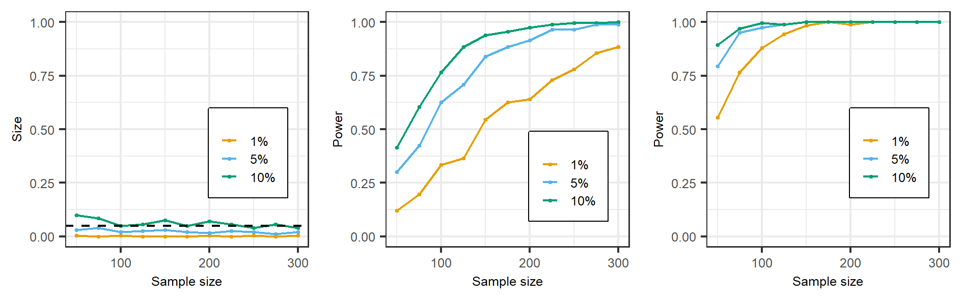
(a) Non-monotone transformation $f_{T}(z_{2})=|z_{2}|$

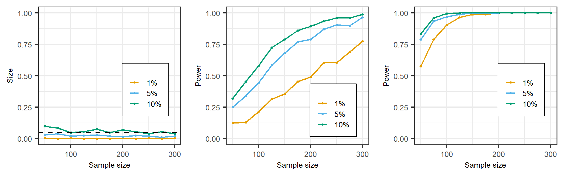
(b) Non-monotone transformation $f_{T}(z_{2})=\mathrm{I}(|z_{2}|<-\Phi^{-1}(0.25))$

(c) Notes: Figures on the left examine size control of the $pdCov$ test of MDep relevance. Figures in the middle and on the right examine the power of the test at $\lambda=0.5$ and $\lambda=1$ respectively. $\Phi^{-1}(0.25)$ denotes the first quartile of the standard normal distribution. The black dashed lines in the graphs on the left correspond to size $=0.05$.

The graphs on the left in Figures 1(a) and 1(b) demonstrate good size control across all sample sizes and nominal levels considered. Graphs in the middle and right of Figure 1(c) demonstrate the test’s ability to detect the presence of non-linear/non-monotone MDep relevance. As expected, power increases in $\lambda$.

E.5 Specification testing

The distance covariance test proposed by [60] is a test of independence. [56] extends the dCov to test conditional mean independence between observed random variables. [58] derives a test from [56]’s shao2014martingale measure which applies to specification testing. Assumption 2(a) is a weak exclusion restriction. [58]’s su2017martingale test applies to conditional mean models of the form $y=g(\mathbf{x};\bm{\theta})+u$ where $\mathbb{E}[y|\mathbf{x}]=g(\mathbf{x};\bm{\theta})$. The test remains applicable whether the researcher uses excluded instruments or not.

The null hypothesis of interest is $\mathbb{H}_{0}:\mathbb{P}\big{(}\mathbb{E}[y_{i}|\mathbf{x}_{i}]=g(\mathbf{x}_{i},\bm{\theta}_{o},\theta_{o,c})\big{)}=1$ against the alternative hypothesis $\mathbb{H}_{1}:\mathbb{P}\big{(}\mathbb{E}[y_{i}|\mathbf{x}_{i}]=g(\mathbf{x}_{i},\bm{\theta},\theta_{c}(\bm{\theta}))\big{)}\big{)}<1$ for any $\bm{\theta}\in\bm{\Theta}$. Let $\hat{u}_{i}$ be the residual corresponding to observation $i$ such that $\sum_{i=1}^{n}\hat{u}_{i}=0$. [58]’s su2017martingale test statistic is given by

$$T_{n}=-\frac{1}{n}\sum_{i\not=j}\sum_{j\not=i}\hat{u}_{i}\hat{u}_{j}||\mathbf{z}_{i}-\mathbf{z}_{j}||$$

Details of the the wild bootstrap used to implement the test as in [58] are described in Section E.6.

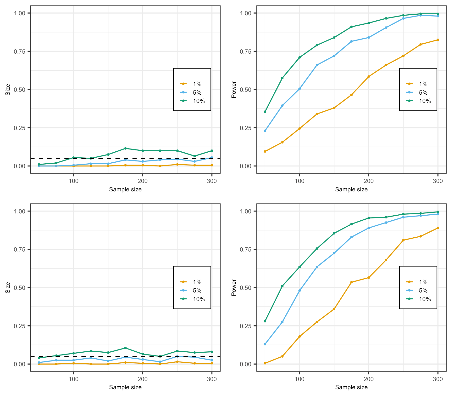
Figure 2: Size & Power - Specification test

(a) Notes: Figures on the left examine size control of [58]’s su2017martingale specification test while the figures on the right examine its power. The graphs on top correspond to specification (v) and the graphs below correspond to specification (i) in Section E.1. The black dashed lines in the graphs on the left correspond to size $=0.05$.

It is instructive to use simulations to verify the performance of [58]’s su2017martingale specification test in the context of the MDep estimator. The specifications (under the null of exogeneity) considered are specifications (v) in Section 4 and (i) in Section E.1. The power of the test is examined under endogeneity using $x_{1}=(\dot{x}+u)/\sqrt{2}$ where $\mathrm{cov}(\dot{x},x^{*})=0.25$ and $\mathrm{cov}(\dot{x},u)=0$. Figure 2(a) presents the size and power of the test at nominal levels 1%, 5%, and 10%.

In all specifications considered, one observes good size control and non-trivial power. In sum, [58]’s su2017martingale specification test is reliable in assessing, among other sources of miss-specification, violations of the sufficient conditional mean independence condition in the MDep setting.

E.6 Implementing the wild bootstrap

Below is an outline of the wild-bootstrap procedure used in conducting the [58] specification test. Define the transformation $\mathcal{T}(\hat{u}_{i})=\sqrt{n/(n-p_{\theta}-1)}\hat{u}_{i}$. The bootstrap errors are sampled from Mammen’s two-point distribution

$$\nu_{i}^{*}=\begin{cases}-(\sqrt{5}-1)/2&\text{with probability }(\sqrt{5}+1)/(2\sqrt{5})\\ (\sqrt{5}+1)/2&\text{with probability }(\sqrt{5}-1)/(2\sqrt{5})\end{cases}$$

for which $\mathbb{E}[\nu_{i}^{*}]=0$, $\mathbb{E}[\nu_{i}^{*2}]=1$, and $\mathbb{E}[\nu_{i}^{*3}]=1$ (see [54]). Other distributions with the same properties can be found in [53]. The bootstrap procedure is specified below.

Algorithm 1.

1. 1. Regress $y_{i}$ on $\mathbf{x}_{i}$. Obtain $\hat{\bm{\theta}}_{n}$ and $u_{i}(\bm{\hat{\bm{\theta}}}_{n})=y_{i}-g(\mathbf{x}_{i},\hat{\bm{\theta}}_{n},\theta_{c}(\hat{\bm{\theta}}_{n}))$

   2. Compute $\hat{u}_{i}=u_{i}(\bm{\hat{\bm{\theta}}}_{n})-\mathbb{E}_{n}[u_{i}(\bm{\hat{\bm{\theta}}}_{n})]$ and the test statistic $T_{n}$

2. For $b=1,\ldots,B$, Do

   1. Generate $y_{i}^{*b}=g(\mathbf{x}_{i},\hat{\bm{\theta}}_{n},\theta_{c}(\hat{\bm{\theta}}_{n}))+\mathbb{E}_{n}[u_{i}(\bm{\hat{\bm{\theta}}}_{n})]+\mathcal{T}(\hat{u}_{i})\nu_{i}^{*b}$

   2. Regress $y_{i}^{*b}$ on $\mathbf{x}_{i}$ and obtain $\hat{\bm{\theta}}_{n}^{*b}$, $u_{i}(\hat{\bm{\theta}}_{n}^{*b})=y_{i}^{*b}-g(\mathbf{x}_{i},\hat{\bm{\theta}}_{n}^{*b})$, $\hat{u}_{i}^{*b}=u_{i}(\bm{\hat{\bm{\theta}}}_{n}^{*b})-\mathbb{E}_{n}[u_{i}(\bm{\hat{\bm{\theta}}}_{n}^{*b})]$, and the test statistic $T_{n}^{*b}$

3. End Do

The p-value of the specification test is computed using $\frac{1}{B}\sum_{b=1}^{B}\mathrm{I}(T_{n}^{*b}>T_{n})$. Testing MDep-relevance using [59]’s szekely2014partial partial distance covariance test requires modifying Algorithm 1. The MDep-relevance test proceeds by replacing $\hat{u}_{i}$ with $\check{x}_{i}=x_{i}-\mathbb{E}_{n}[x_{i}]$, generating bootstrap samples as $\check{x}_{i}^{*b}=\mathcal{T}(\check{x}_{i})\nu_{i}^{*b}$, skipping regression steps, and computing the p-value as $\frac{1}{B}\sum_{b=1}^{B}\mathrm{I}(pdC_{n}^{*b}>pdC_{n})$. Conducting a $pdCov$ test of non-linear relevance only requires replacing $\check{x}_{i}$ with residuals from a linear projection of $\mathbf{x}_{2}$ on $\mathbf{z}_{2}$. Computation of the dCov and partial dCov measures is done using the energy R package [55].

References

- [1] Donald WK Andrews “Consistency in nonlinear econometric models: A generic uniform law of large numbers” In Econometrica: Journal of the Econometric Society JSTOR, 1987, pp. 1465–1471
- [2] Donald WK Andrews, Marcelo J Moreira and James H Stock “Optimal two-sided invariant similar tests for instrumental variables regression” In Econometrica 74.3 Wiley Online Library, 2006, pp. 715–752
- [3] Isaiah Andrews and Timothy B Armstrong “Unbiased instrumental variables estimation under known first-stage sign” In Quantitative Economics 8.2 Wiley Online Library, 2017, pp. 479–503
- [4] Isaiah Andrews and Anna Mikusheva “Conditional inference with a functional nuisance parameter” In Econometrica 84.4 Wiley Online Library, 2016, pp. 1571–1612
- [5] Isaiah Andrews, James H Stock and Liyang Sun “Weak instruments in instrumental variables regression: Theory and practice” In Annual Review of Economics 11 Annual Reviews, 2019, pp. 727–753
- [6] Alexandre Belloni, Daniel Chen, Victor Chernozhukov and Christian Hansen “Sparse models and methods for optimal instruments with an application to eminent domain” In Econometrica 80.6 Wiley Online Library, 2012, pp. 2369–2429
- [7] Dennis S Bernstein “Matrix Mathematics: Theory, Facts, and Formulas” Princeton University Press, 2009
- [8] John Bound, David A Jaeger and Regina M Baker “Problems with instrumental variables estimation when the correlation between the instruments and the endogenous explanatory variable is weak” In Journal of the American Statistical Association 90.430 Taylor & Francis, 1995, pp. 443–450
- [9] Jiafeng Chen, Daniel L Chen and Greg Lewis “Mostly Harmless Machine Learning: Learning Optimal Instruments in Linear IV Models” In arXiv preprint arXiv:2011.06158, 2020
- [10] Xu Cheng and Zhipeng Liao “Select the valid and relevant moments: An information-based lasso for gmm with many moments” In Journal of Econometrics 186.2 Elsevier, 2015, pp. 443–464
- [11] Victor Chernozhukov and Christian Hansen “Instrumental quantile regression inference for structural and treatment effect models” In Journal of Econometrics 132.2 Elsevier, 2006, pp. 491–525
- [12] Victor Chernozhukov and Christian Hansen “Instrumental variable quantile regression: A robust inference approach” In Journal of Econometrics 142.1 Elsevier, 2008, pp. 379–398
- [13] Richard A Davis, Muneya Matsui, Thomas Mikosch and Phyllis Wan “Applications of distance correlation to time series” In Bernoulli 24.4A Bernoulli Society for Mathematical StatisticsProbability, 2018, pp. 3087–3116
- [14] Steven G Dieterle and Andy Snell “A simple diagnostic to investigate instrument validity and heterogeneous effects when using a single instrument” In Labour Economics 42 Elsevier, 2016, pp. 76–86
- [15] Dominic Edelmann, Konstantinos Fokianos and Maria Pitsillou “An updated literature review of distance correlation and its applications to time series” In International Statistical Review 87.2 Wiley Online Library, 2019, pp. 237–262
- [16] Kathryn Graddy “Testing for imperfect competition at the Fulton fish market” In The RAND Journal of Economics JSTOR, 1995, pp. 75–92
- [17] Christian Hansen and Damian Kozbur “Instrumental variables estimation with many weak instruments using regularized JIVE” In Journal of Econometrics 182.2 Elsevier, 2014, pp. 290–308
- [18] Keisuke Hirano and Jack R Porter “Location properties of point estimators in linear instrumental variables and related models” In Econometric Reviews 34.6-10 Taylor & Francis, 2015, pp. 720–733
- [19] Wassily Hoeffding “A Class of Statistics with Asymptotically Normal Distribution” In The Annals of Mathematical Statistics 19.3, 1948, pp. 293–325 DOI: 10.1214/aoms/1177730196
- [20] Erik Hornung “Immigration and the diffusion of technology: The Huguenot diaspora in Prussia” In American Economic Review 104.1, 2014, pp. 84–122
- [21] Peter J Huber “The behavior of maximum likelihood estimates under nonstandard conditions” In Proceedings of the fifth Berkeley symposium on mathematical statistics and probability 1.1, 1967, pp. 221–233 University of California Press
- [22] Frank Kleibergen and Richard Paap “Generalized reduced rank tests using the singular value decomposition” In Journal of Econometrics 133.1 Elsevier, 2006, pp. 97–126
- [23] Roger Koenker and Gilbert Bassett Jr “Regression quantiles” In Econometrica: Journal of the Econometric Society JSTOR, 1978, pp. 33–50
- [24] Sokbae Lee “Endogeneity in quantile regression models: A control function approach” In Journal of Econometrics 141.2 Elsevier, 2007, pp. 1131–1158
- [25] Runze Li, Wei Zhong and Liping Zhu “Feature screening via distance correlation learning” In Journal of the American Statistical Association 107.499 Taylor & Francis, 2012, pp. 1129–1139
- [26] Charles R Nelson and Richard Startz “The distribution of the instrumental variables estimator and its t-ratio when the instrument is a poor one” In Journal of business JSTOR, 1990, pp. S125–S140
- [27] Charles R. Nelson and Richard Startz “Some Further Results on the Exact Small Sample Properties of the Instrumental Variable Estimator” In Econometrica 58.4 [Wiley, Econometric Society], 1990, pp. 967–976
- [28] Whitney K Newey and Daniel McFadden “Large sample estimation and hypothesis testing” In Handbook of Econometrics 4 Elsevier, 1994, pp. 2111–2245
- [29] Walter Oberhofer and Harry Haupt “Asymptotic theory for nonlinear quantile regression under weak dependence” In Econometric Theory 32.3 Cambridge University Press, 2016, pp. 686
- [30] José Luis Montiel Olea and Carolin Pflueger “A robust test for weak instruments” In Journal of Business & Economic Statistics 31.3 Taylor & Francis Group, 2013, pp. 358–369
- [31] Ariel Pakes and David Pollard “Simulation and the asymptotics of optimization estimators” In Econometrica: Journal of the Econometric Society JSTOR, 1989, pp. 1027–1057
- [32] Trevor Park, Xiaofeng Shao and Shun Yao “Partial martingale difference correlation” In Electronic Journal of Statistics 9.1 The Institute of Mathematical Statisticsthe Bernoulli Society, 2015, pp. 1492–1517
- [33] David Pollard “New ways to prove central limit theorems” In Econometric Theory JSTOR, 1985, pp. 295–313
- [34] James L Powell “Estimation of monotonic regression models under quantile restrictions” In Nonparametric and semiparametric methods in Econometrics Cambridge University Press Cambridge, 1991, pp. 357–384
- [35] Eleanor Sanderson and Frank Windmeijer “A weak instrument F-test in linear IV models with multiple endogenous variables” In Journal of Econometrics 190.2 Elsevier, 2016, pp. 212–221
- [36] Xiaofeng Shao and Jingsi Zhang “Martingale difference correlation and its use in high-dimensional variable screening” In Journal of the American Statistical Association 109.507 Taylor & Francis, 2014, pp. 1302–1318
- [37] Wenhui Sheng and Xiangrong Yin “Direction estimation in single-index models via distance covariance” In Journal of Multivariate Analysis 122 Elsevier, 2013, pp. 148–161
- [38] Douglas Staiger and James H. Stock “Instrumental Variables Regression with Weak Instruments” In Econometrica 65.3 [Wiley, Econometric Society], 1997, pp. 557–586
- [39] James Stock and Motohiro Yogo “Testing for Weak Instruments in Linear IV Regression” In Identification and Inference for Econometric Models New York: Cambridge University Press, 2005, pp. 80–108 Cambridge University Press
- [40] Liangjun Su and Xin Zheng “A martingale-difference-divergence-based test for specification” In Economics Letters 156 Elsevier, 2017, pp. 162–167
- [41] Gábor J Székely and Maria L Rizzo “Brownian distance covariance” In The Annals of Applied Statistics JSTOR, 2009, pp. 1236–1265
- [42] Gábor J Székely and Maria L Rizzo “On the uniqueness of distance covariance” In Statistics & Probability Letters 82.12 Elsevier, 2012, pp. 2278–2282
- [43] Gábor J Székely and Maria L Rizzo “Partial distance correlation with methods for dissimilarities” In The Annals of Statistics 42.6 Institute of Mathematical Statistics, 2014, pp. 2382–2412
- [44] Gábor J Székely, Maria L Rizzo and Nail K Bakirov “Measuring and testing dependence by correlation of distances” In The Annals of Statistics 35.6 Institute of Mathematical Statistics, 2007, pp. 2769–2794
- [45] Aad W Van der Vaart “Asymptotic statistics” Cambridge university press, 1998
- [46] Jeffrey M Wooldridge “Econometric analysis of cross section and panel data” MIT Press, 2010
- [47] Kai Xu and Fangxue Chen “Martingale-difference-divergence-based tests for goodness-of-fit in quantile models” In Journal of Statistical Planning and Inference 207 Elsevier, 2020, pp. 138–154
- [48] Wei Zhong and Liping Zhu “An iterative approach to distance correlation-based sure independence screening” In Journal of Statistical Computation and Simulation 85.11 Taylor & Francis, 2015, pp. 2331–2345
- [49] Zhou Zhou “Measuring nonlinear dependence in time-series, a distance correlation approach” In Journal of Time Series Analysis 33.3 Wiley Online Library, 2012, pp. 438–457
- [50] James Davidson “Stochastic limit theory: An introduction for econometricians” OUP Oxford, 1994
- [51] Peter Hall and Simon J Sheather “On the distribution of a studentized quantile” In Journal of the Royal Statistical Society: Series B (Methodological) 50.3 Wiley Online Library, 1988, pp. 381–391
- [52] Frank Kleibergen and Richard Paap “Generalized reduced rank tests using the singular value decomposition” In Journal of Econometrics 133.1 Elsevier, 2006, pp. 97–126
- [53] Regina Y Liu “Bootstrap procedures under some non-iid models” In The Annals of Statistics 16.4 Institute of Mathematical Statistics, 1988, pp. 1696–1708
- [54] Enno Mammen “Bootstrap and wild bootstrap for high dimensional linear models” In The Annals of Statistics JSTOR, 1993, pp. 255–285
- [55] Maria Rizzo and Gabor Szekely “energy: E-Statistics: Multivariate Inference via the Energy of Data” R package version 1.7-7, 2019 URL: https://CRAN.R-project.org/package=energy
- [56] Xiaofeng Shao and Jingsi Zhang “Martingale difference correlation and its use in high-dimensional variable screening” In Journal of the American Statistical Association 109.507 Taylor & Francis, 2014, pp. 1302–1318
- [57] James Stock and Motohiro Yogo “Testing for Weak Instruments in Linear IV Regression” In Identification and Inference for Econometric Models New York: Cambridge University Press, 2005, pp. 80–108 Cambridge University Press
- [58] Liangjun Su and Xin Zheng “A martingale-difference-divergence-based test for specification” In Economics Letters 156 Elsevier, 2017, pp. 162–167
- [59] Gábor J Székely and Maria L Rizzo “Partial distance correlation with methods for dissimilarities” In The Annals of Statistics 42.6 Institute of Mathematical Statistics, 2014, pp. 2382–2412
- [60] Gábor J Székely, Maria L Rizzo and Nail K Bakirov “Measuring and testing dependence by correlation of distances” In The Annals of Statistics 35.6 Institute of Mathematical Statistics, 2007, pp. 2769–2794