Asymmetric Heavy Tails and Implicit Bias in Gaussian Noise Injections
Asymmetric Heavy Tails and Implicit Bias in Gaussian Noise Injections
SUPPLEMENTARY DOCUMENT
Abstract
Gaussian noise injections (GNIs) are a family of simple and widely-used regularisation methods for training neural networks where one injects additive or multiplicative Gaussian noise to the network activations at every iteration of the optimisation algorithm, which is typically chosen as stochastic gradient descent (SGD). In this paper we focus on the so-called ‘implicit effect’ of GNIs, which is the effect of the injected noise on the dynamics of SGD. We show that this effect induces an asymmetric heavy-tailed noise on SGD gradient updates. In order to model this modified dynamics, we first develop a Langevin-like stochastic differential equation that is driven by a general family of asymmetric heavy-tailed noise. Using this model we then formally prove that GNIs induce an ‘implicit bias’, which varies depending on the heaviness of the tails and the level of asymmetry. Our empirical results confirm that different types of neural networks trained with GNIs are well-modelled by the proposed dynamics and that the implicit effect of these injections induces a bias that degrades the performance of networks.
[pdftoc]hyperrefToken not allowed in a PDF string \WarningFilter[xclr]xcolorIncompatible color definition \ActivateWarningFilters[pdftoc] \ActivateWarningFilters[xclr]
1 Introduction
Noise injections are a family of methods that involve adding or multiplying samples from a noise distribution to the weights and activations of a neural network during training. The most commonly used distributions are Bernoulli distributions and Gaussian distributions (Srivastava et al., 2014; Poole et al., 2014) and the noise is most often inserted at the level of network activations.
Though the regularisation conferred by Gaussian noise injections (GNIs) can be observed empirically, and there have been many studies on the benefits of noising data (Bishop, 1995; Cohen et al., 2019; Webb, 1994), the mechanisms by which these injections operate are not fully understood. Recently, the explicit effect of GNIs, which is the added term to the loss function obtained when marginalising out the injected noise, has been characterised analytically (Camuto et al., 2020): it corresponds to a penalisation in the Fourier domain which improves model generalisation.
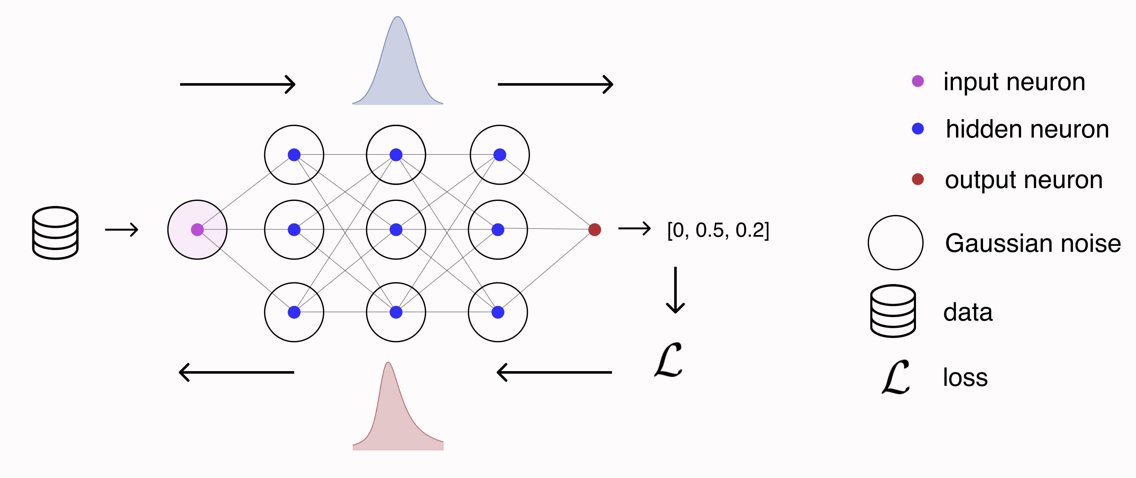
Here we extend this analysis and focus on the implicit effect of GNIs. This is the effect of the remaining noise that has been marginalised out when studying the explicit effect. In particular we focus on the manner in which such noise alters the dynamics of Stochastic Gradient Descent (SGD) (Wei et al., 2020; Zhang et al., 2017). We show that the implicit effect is driven by an asymmetric heavy-tailed noise on the SGD gradient updates, as illustrated in Figure 1.
To study the effect of this gradient noise, we model the dynamics of SGD for a network experiencing GNIs by a stochastic differential equation (SDE) driven by an asymmetric heavy-tailed -stable noise. We demonstrate that this model captures the dynamics of networks trained with GNIs and we show that the stationary distribution of this process becomes arbitrarily distant from the so-called Gibbs measure, whose modes exactly match the local minima of the loss function, as the gradient becomes increasingly heavy-tailed and asymmetric. Heavy-tailed and asymmetric gradient noise thus degrades network performance and this suggests that models trained with the full effect of GNIs will underperform networks trained solely with the explicit effect. We confirm this experimentally for a variety of dense and convolutional networks.111See https://github.com/alexander-camuto/asym-heavy-tails-bias-GNI for all code.
2 Background
Stable Distributions. The Generalised Central Limit Theorem (GCLT) (Gnedenko & Kolmogorov, 1954) states that for a sequence of independent and identically distributed (i.i.d.) random variables whose distribution has a power-law tail with index , the normalised sum converges to a heavy-tailed distribution called the -stable distribution () as the number of summands grows. An -stable distributed random variable is denoted by , where is the tail-index, is the skewness parameter, is the scale parameter, and is called the location parameter. The mean of coincides with if , and otherwise the mean of is undefined. In this work, we always assume . The parameter is a measure of asymmetry. We say that follows a symmetric -stable distribution denoted as if (and ). The parameter determines the tail thickness of the distribution, and measures the spread of around its mode. Note that when , -stable distributions have heavy tails such that their moments are finite only up to the order .
The probability density function (p.d.f.) of an -stable random variable, , does not have a closed-form expression except for a few special cases. When and , the symmetric -stable distribution reduces to the Cauchy and the Gaussian distributions, respectively, (cf. Section 1.1. in (Samorodnitsky & Taqqu, 1994)). By their flexibility, such distributions can model many complex stochastic phenomena for which exact analytic forms are intractable (Sarafrazi & Yazdi, 2019; Fiche et al., 2013).
Lévy Processes. A Lévy process (motion) is a stochastic process with independent, stationary increments. Formally, is Lévy process if
-
(i)
almost surely;
-
(ii)
For any , the increments are independent, ;
-
(iii)
The difference and have the same distribution;
-
(iv)
is continuous in probability, i.e. for any and , as .
The -stable Lévy process is an important class of Lévy processes. In particular, for , let denote the -dimensional -stable Lévy process with independent components, i.e. each component is an independent scalar -stable Levy motion (Duan, 2015) such that has the distribution for any .
Stochastic Gradient Descent and Differential Equations. Let be a training dataset composed of data-label pairs of the form , and let be the parameters of an layer neural network in vector form. When a neural network operates on input data , we obtain the activations , where and where is the number of neurons in the layer: we consider a non-linearity , , where is applied element-wise to each coordinate of its argument. In supervised settings, our objective is to find the optimal parameters that minimise the negative log-likelihood of the labels , given the parameters and data :
| (2.1) |
SGD and its variants are the most prevalent optimisation routines that underpin the training of very large neural networks. Under SGD, we estimate equation (2.1) by sampling a random mini-batch of data-label pairs ,
| (2.2) |
SGD optimises this equation and approximates using iterative parameter updates. At training step
| (2.3) |
where is the step-size for updates (the network’s learning rate) (Robbins & Monro, 1951; Ruder, 2016).
Studying the dynamics of SGD allows us to understand the subtle effects that batching may have on neural network training. The similarities between the SGD algorithm and Langevin diffusions (Roberts & Stramer, 2002) have inspired many studies modelling the dynamics of SGD using stochastic differential equations (SDEs) under different noise conditions (Agapiou et al., 2014; Şimşekli et al., 2019; Raginsky et al., 2017; Gao et al., 2018, 2020; Jastrzȩbski et al., 2017; Li et al., 2017). In this approach, one models the discrete SGD updates (2.3), as the discretisation of a continuous-time stochastic process, making assumptions about the properties of the ‘noise’ that drives this process (Mandt et al., 2016; Jastrzȩbski et al., 2017). This noise stems from the stochasticity in approximating the ‘true’ gradient over the dataset with that of a mini-batch , . We denote this noise as,
| (2.4) |
The most prevalent assumption is that the gradient noise admits a multi-variate Gaussian noise: . This is rationalised by the central limit theorem, as the sum of estimation errors in equation (2.4) is approximately Gaussian for sufficiently large batches. Under this assumption, we can rewrite the SGD parameter update as:
| (2.5) |
Then, one obtains the following continuous-time SDE to approximate the gradient updates (Welling & Teh, 2011; Mandt et al., 2016; Jastrzȩbski et al., 2017):
| (2.6) |
where is the Brownian motion in and is the assumed noise variance for . However, recent work suggests that the Gaussian assumption might not be always appropriate (Gürbüzbalaban et al., 2020; Hodgkinson & Mahoney, 2020), and connectedly, the gradient noise is observed to be heavy-tailed in different settings (Şimşekli et al., 2019; Zhou et al., 2020). Under this noise assumption, the corresponding SDE is such that in (2.6) is replaced with the symmetric stable process where :
| (2.7) |
Gaussian Noise Injections. GNIs are regularisation methods that consist of injecting Gaussian noise to the network activations. More precisely, let be a collection of ‘noise vectors’ injected to the network activations at each layer except the final layer: , where , and is the number of neurons in the layer. We have two values for an activation: the soon-to-be noised value , and the subsequently noised value . For a multi-layer perceptron (MLP),
| (2.8) |
where is some element-wise operation (e.g., addition or multiplication). For additive GNIs typically, , and for multiplicative GNIs we often use , where is the Gaussian distribution. The ‘accumulated’ noise at each layer, induced by the noise injected to the layer and in previous layers is
| (2.9) |
Given that GNIs are commonly used as regularisation methods (Camuto et al., 2020; Dieng et al., 2018; Srivastava et al., 2014; Poole et al., 2014; Kingma et al., 2015; Bishop, 1995), our goal is to understand better the mechanisms by which they affect neural networks.
3 The Implicit Effect of GNIs
Recently, Camuto et al. (2020) showed that the effect of GNIs on the cost function can be expressed as a term that is added to the loss, i.e.,
| (3.1) |
where is the modified loss that SGD ultimately aims to minimise. The term can be further broken down into explicit and implicit effects, as described in Section 1.
We build on the approach of Camuto et al. (2020) and define the explicit effect as the additional term obtained on the loss when we marginalise out the noise we have injected. It offers a consistently positive objective for gradient descent to optimise and we denote it as . The implicit effect is then the remainder of the terms marginalised out in the explicit effect:
| (3.2) |
While the explicit effect focuses on the consistent and non-stochastic regularisation induced by GNIs, the implicit effect instead studies the effect of the inherent stochasticity of GNIs. This term does not offer a consistent objective for SGD to minimise. Rather we show that it affects neural network training by way of the heavy-tailed and skewed noise it induces on gradient updates.
Subsequently, we first characterise the tail properties of the noise accumulated during the forward pass. As this accumulated noise defines the implicit effect we can then use this result to show that gradients induced by the implicit effect are heavy-tailed and skewed and apt to be modelled by heavy-tailed and asymmetric -stable noise.
The Properties of the Accumulated Noise. Before considering the properties of the implicit effect gradients, we first need to study the noise that is accumulated during the forward pass of a neural network experiencing GNIs. Here we use asymptotic analysis to bound the moments of this noise, allowing us to characterise the tail properties of gradients using the broad class of sub-Weibull distributions that include a range of heavy-tailed distributions (Vladimirova et al., 2019, 2020; Kuchibhotla & Chakrabortty, 2018).
Definition 3.1.
(Asymptotic order) A positive sequence is of the same order as another positive sequence () if such that . is of the same order of magnitude as (, i.e. ‘asymptotically equivalent’) if there exist some such that: for any .
Definition 3.2.
(Sub-Weibull distributions), : We say that a random variable is sub-Weibull (Vladimirova et al., 2020; Kuchibhotla & Chakrabortty, 2018) with tail parameter if , where . In this case, we write . Such distributions satisfy the tail bound , where is some constant. Note that for and we recover the sub-Gaussian and sub-exponential families and that if , then for .
As increases the tail distribution becomes heavier-tailed. To simplify our analysis we consider activation functions that obey the extended envelope property.
Definition 3.3 (Extended Envelope Property (Vladimirova et al., 2019):).
A non-linear function is said to obey the extended envelope property if such that:
-
•
, for any or ;
-
•
, for any .
Activation functions that obey this property, such as , are broadly moment preserving (Vladimirova et al., 2020). Using this property, we can characterise the moments for the noised activation in a layer , .
Lemma 3.1.
For feed-forward neural networks with an activation function that obeys the extended envelope property, the noised activations at each layer , resulting from additive-GNIs obey
For multiplicative-GNIs we have,
where is the dimensionality of the layer.
Lemma 3.1 shows that when the injected noise is additive, the noised activations at each layer will have (sub)-Gaussian tails. By equation (2.9), the accumulated noise will also have sub-Gaussian tails as the non-noised activations are deterministic and do not affect the asymptotic relationships of moments. See Figure A.1 of the Appendix for a demonstration that the activations experience Gaussian-like noise for additive-GNIs. For multiplicative-GNIs the noise at each layer, except the input layer which experiences Gaussian noise, behaves with a sub-Weibull tail. We demonstrate this behaviour in Figure A.2 of the Appendix.
We can now study the properties of the gradient noise induced by the implicit effect by taking the gradients of this forward pass noise.
Kurtosis of The Gradient Noise. We characterise the gradient noise corresponding to , the weight that maps from neuron in layer to neuron in layer .
Theorem 3.1.
Consider a feed-forward neural network with an activation function that obeys the extended envelope property and a cross-entropy or mean-squared-error cost (see Appendix B). The gradient noise from additive-GNIs , has zero mean and has moments that obey for a pair :
where is defined in (3.2). For multiplicative GNIs, we have
For the additive noise, these bounds infer that the gradient noise at each layer will have sub-exponential tails. For the multiplicative case, gradient noise will be sub-Weibull, with a tail parameter that increases with the layer index. Unlike the forward pass, which experienced noise bounded in its tails by a Gaussian, the backward pass experiences noise that is bounded in its tails by heavy-tailed Weibull distributions with tail parameter .
Remark 3.1.
Our result applies to the gradient for a single pair . During SGD, we take the mean gradient across a batch of size . To study the tail distribution of this mean gradient, we restate in a simplified manner Kuchibhotla & Chakrabortty (2018)’s generalisation of the Bernstein inequality for zero-mean sub-Weibull random variables in Theorem 3.2.
Theorem 3.2 (Theorem 3.1 in Kuchibhotla & Chakrabortty (2018)).
Let be independent mean-zero sub-Weibull random variables with a shared tail parameter . Then, for every , we have
where are constants that depend on the tail parameter and where
| (3.3) |
is the ‘sub-Weibull norm’.
This theorem states that the the tails of the mean of zero-mean i.i.d. sub-Weibull random variables are produced by a single variable, say , with the maximal sub-Weibull norm , i.e., the one with the heaviest tails. Assuming gradients are independent across data points, we can use this inequality to bound the tail probability for the sum of our zero-mean gradients. If a single gradient is sufficiently heavy-tailed, then the mean across the batch will also be heavy-tailed.
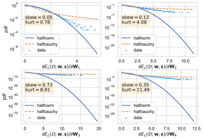
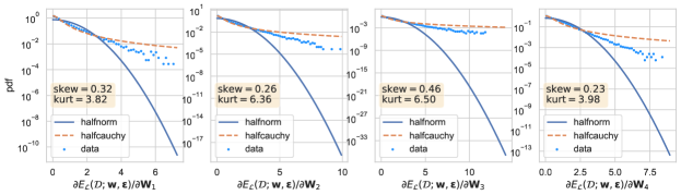
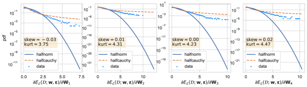
In Figure 2 we show that the implicit effect gradient, averaged over the entire dataset (i.e., the largest batch-size possible), is heavy-tailed, unlike the forward pass. To calculate these gradients, we estimate the explicit regulariser in equation (3.2) using Monte Carlo sampling, , similarly to (Wei et al., 2020; Camuto et al., 2020). We show these results for multiplicative-GNIs in Figure A.3 of the Appendix. In this setting as well, the backward pass experiences heavy-tailed noise from GNIs.
Skewness of The Gradient Noise. In the proof of Theorem 3.1 we decompose as , where is the (noised) activation of the neuron in the layer. Both these derivatives are likely to be skewed due to the asymmetry of the activation functions and their gradients. Ignoring potential correlations between variables, we observe that product of two zero-mean skewed independent variables and is also skewed . The skewness of the derivatives in the backward pass will induce skewed gradient noise, as seen in Figure 2. Though correlations between gradients could also cause skewness, we show that this is not the case in Appendix C.
4 An SDE Model for SGD with GNIs.
In this section, we will analyse the effects of the skewed and heavy-tailed noise on the SGD dynamics. Recall that the modified loss function by the GNIs is the sum of the explicit regulariser and the original loss over the dataset ,
and the SGD recursion takes the following form:
| (4.1) |
where is given as follows:
| (4.2) | ||||
To ease the notation, let us denote the modified loss function by .
Remark 4.1.
Note that when the gradients are computed over the whole dataset , the gradient noise solely stems from the implicit effect, .
Recent studies have proven that heavy-tailed behaviour can already emerge in stochastic optimisation (without GNIs) (Hodgkinson & Mahoney, 2020; Gürbüzbalaban et al., 2020; Gürbüzbalaban & Hu, 2020), which can further result in an overall heavy-tailed behaviour in the gradient noise, as empirically reported in (Şimşekli et al., 2019; Zhang et al., 2020; Zhou et al., 2020). Accordingly, (Şimşekli et al., 2019; Zhou et al., 2020) proposed modelling the gradient noise by using a centred symmetric -stable noise, which then paved the way for modelling the SGD dynamics by using an SDE driven by a symmetric -stable process (see (2.7)).
We take a similar route for modelling the trajectories of SGD with GNIs; however, due to the skewness arising from the GNIs, the symmetric noise assumption is not appropriate for our purposes. Hence, we propose modelling the skewed gradient noise (4.2) by using an asymmetric -stable noise, which aims at modelling both the heavy-tailed behaviour and the asymmetries at the same time. In particular, we consider an SDE driven by an asymmetric stable process and its Euler discretisation as follows:
| (4.3) | ||||
| (4.4) |
where is the -dimensional skewness and each coordinate can have its idiosyncratic skewness . is a -dimensional asymmetric -stable Lévy process with independent components, and encapsulates all the scaling parameters. Furthermore, denotes the sequence of step-sizes, which can be taken as constant or decreasing, and finally is a sequence of i.i.d. random vectors where each component of is i.i.d. with . We then propose the discretised process (4.4) as a proxy to the original recursion (4.1) and we will directly analyse the theoretical properties of (4.4). Note that our approach strictly extends (Şimşekli et al., 2019), which appears as a special case when .
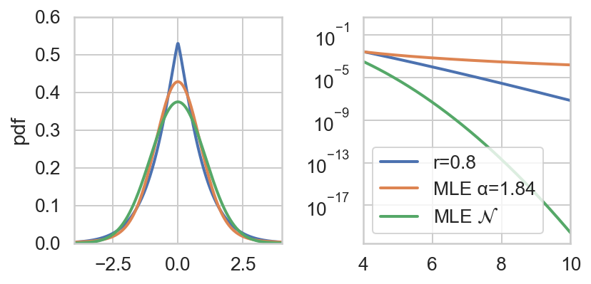
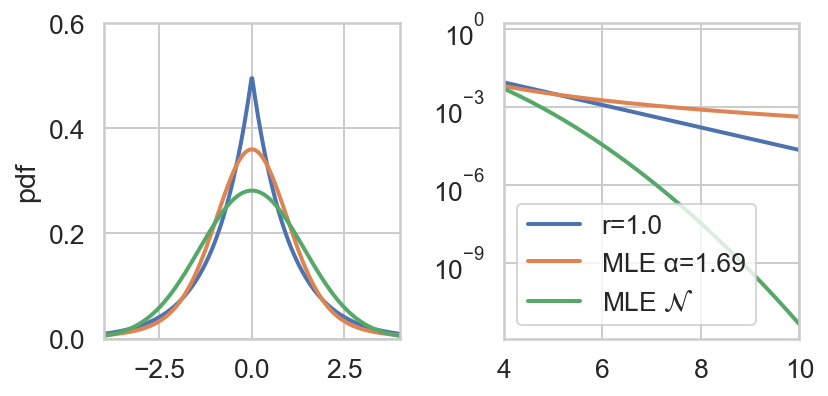
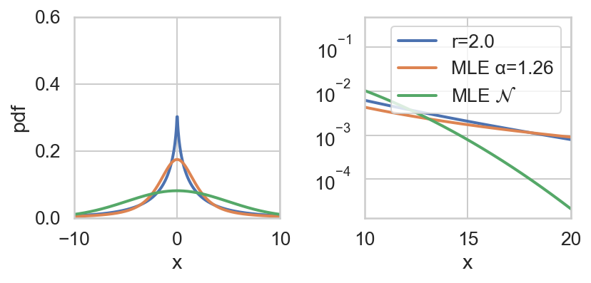
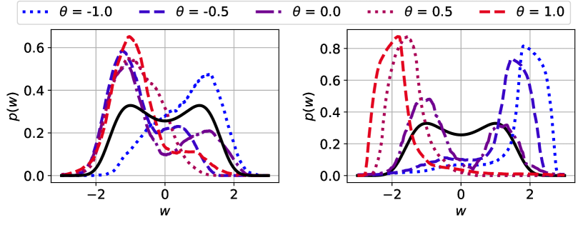
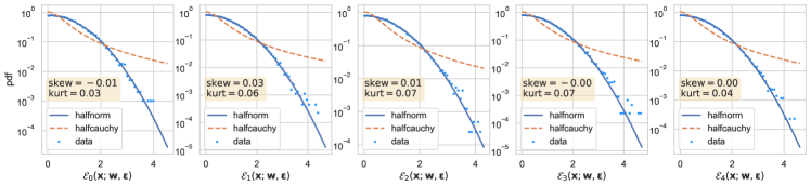
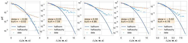
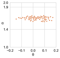
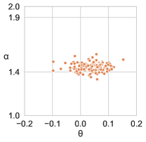
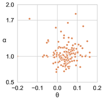
Before deriving our theoretical results, we first verify empirically that the proxy dynamics (4.4) are indeed a good model for representing (4.1). We ascertain that is sufficiently general in the sense that it can capture the gradient noise induced by the implicit effect even when there is no batching noise (when the batch size approaches the size of the dataset for example, see Remark 4.1). As a first line of evidence, in Figure A.4 of the Appendix we model as being drawn from a univariate . The equivalent distributions are skewed () and heavy-tailed (), demonstrating that captures the core properties of the implicit effect gradients highlighted in Section 3. To illustrate this more clearly, in Figure 3 we use symmetric sub-Weibull distributions with , and fit and Gaussians () using maximum likelihood (MLE) from samples. We plot the MLE densities, and clearly MLE () better model the tails of the sub-Weibulls than a Gaussian distribution, even for which is close to Gaussian tails (). The modelling of the tails improves as increases. This further illustrates the appropriateness of our noise model.
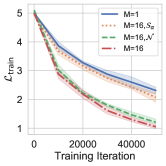
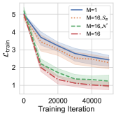
In Figure 4, we further show that the gradient noise of the implicit effect and gradient noise drawn from an equivalent distribution will have similar effects on gradient descent. We sample GNI samples and evaluate:
| (4.5) |
The objective is over the entire dataset such that we eliminate noise from the batching process. allows us to control the ‘degree’ to which the implicit effect is marginalised out. corresponds to the usual training with GNI and larger values of mimic the effects of marginalising out the implicit effect. We model for as being drawn from a univariate or a univariate normal distribution and estimate distribution parameters using maximum likelihood estimation, as in (Nolan, 2001), at each training iteration. We add draws from the estimated distributions to the gradients of models to mimic the combined implicit and explicit effects. models with the added noise have the same training path as models, whereas those with Gaussian gradient noise do not. Thus, distributions are able to faithfully capture the dynamics induced by the implicit effect on gradient descent.
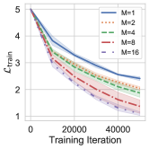
In these same experiments models outperform models on training data. We refine this study for a greater range of values in Figure 5. As increases, performance of models on training data improves gradually, suggesting that the implicit effect degrades performance. Further, in Figure 4, models trained with Gaussian noise added to gradients outperform models, suggesting that the heavy-tails and skew of the implicit effect gradients are responsible for this performance degradation. We now study this apparent bias.

Theoretical analysis of implicit bias. Due to their heavy-tailed nature, stable processes have significantly different statistical properties from those of their Brownian counterparts. Their trajectories have a countable number of discontinuities, called jumps, whereas Brownian motion is continuous almost everywhere. With these jumps the process can escape from ‘narrow’ basins and spend more time in ‘wider’ basins (see Appendix F for the definition of width). Theoretical results demonstrating this have been provided for symmetric stable processes () (Şimşekli et al., 2019). By translating the related metastability results from statistical physics (Imkeller & Pavlyukevich, 2008) to our context, in Appendix F we illustrate that this also holds for SDEs driven by asymmetric stable processes (). In this sense, the SDE (4.3) is ‘biased’ towards wider basins.
While driving SGD iterates towards wider minima could be beneficial, we now show that heavy tails can also introduce an undesirable bias and that this bias is magnified by asymmetries. To quantify this bias, we focus on the invariant measure (i.e., the stationary distribution) of the Markov process (4.4) and investigate its modes (i.e., its local maxima), around where the process resides most of the time.
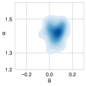
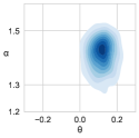
In a statistical physics context, Dybiec et al. (2007) empirically illustrated that the asymmetric stable noise can cause ‘shifts’, in the sense that the modes of the stationary distribution of (4.4) can shift away from the true local minima of , which are of our interest as our aim is to minimise . They further illustrated that such shifts can be surprisingly large when gets smaller and gets larger. We illustrate this outcome by reproducing one of the experiments provided in (Dybiec et al., 2007) in Figure 6. Here, we consider a one-dimensional problem with the quartic potential , and simulate (4.4) for K iterations with constant step-size and . By using the generated iterates, we estimate the density of the invariant measure of (4.4) by using the kernel density estimator provided in - (Pedregosa et al., 2011), for different values of and . When is larger (left), the heavy-tails cause a shift in the modes of the invariant measure, where these shifts become slightly larger with increasing asymmetries (). When the tails are heavier (right), we observe a much stronger interaction between and , and observe drastic shifts as the asymmetry is increased.
From an optimisation perspective, these results are rather unsettling as they imply that SGD might spend most of its time in regions that are arbitrarily far from the local minima of the objective function , since the high probability regions of its stationary distribution might be shifted away from the local minima of interest. In the symmetric case (), this observation has been formally proven in (Sliusarenko et al., 2013) when is chosen as the one dimensional quartic potential of Figure 6 and when . A direct quantification of such shifts is non-trivial; and in the presence of asymmetries (), even further difficulties emerge.
In a recent study Şimşekli et al. (2020) focused on eliminating the undesired bias introduced by symmetric stable noise in SGD with momentum (Qian, 1999), and proposed an indirect way to ensure that modes of the stationary distribution exactly match the objective function’s local minima. They developed a ‘modified’ SDE whose invariant distribution can be proven to be the Gibbs measure, denoted by , which is a probability measure that has a density proportional to for some . Clearly, all the local maxima of this density coincide with the local minima of the function ; hence, their approach eliminates the possibility of a shift in the modes by imposing a stronger condition which controls the entire invariant distribution.
By following a similar approach, we will bound the gap between the invariant measure of (4.4) and the Gibbs measure in terms of the tail index and the skewness , using it as a quantification of the bias induced by the asymmetric heavy-tailed noise. In particular, for any sufficiently regular test function , we consider its expectation under the Gibbs measure , and its sample average computed over (4.4), i.e., , where . We then bound the weak error: , whose convergence to zero is sufficient for ensuring the modes do not shift.
We derive this bound for our case in three steps: (i) We first link the discrete-time process (4.4) to its continuous-time limit (4.3) by directly using the results of (Panloup, 2008). (ii) We then design a modified SDE that has the unique invariant measure as the Gibbs measure, with all the modes matching those of the loss function (Theorem 4.1). (iii) Finally, we show that the SDE (4.3) is a poor numerical approximation to the modified SDE, and we develop an upper-bound for the approximation error (Theorem 4.2).
To address (ii), we introduce a modification to (4.3), coined asymmetric fractional Langevin dynamics:
| (4.6) |
where, the drift function is defined as follows:
| (4.7) |
where , , , and . Here, the operator denotes a Riesz-Feller type fractional derivative (Gorenflo & Mainardi, 1998; Mainardi et al., 2001) whose exact (and rather complicated) definition is not essential in our problematic, and is given in Appendix E in order to avoid obscuring the main results. The next theorem states that the SDE (4.6) targets the Gibbs measure.
Theorem 4.1.
This theorem states that the use of the modified drift in place of , prevents any potential shifts in the modes of the invariant measure.
The fractional derivative in (4.7) is a non-local operator that requires the knowledge of the full function, and does not admit a closed-form expression. In the next step, we develop an approximation scheme for the drift in (4.6), and show that the gradient in (4.4) appears as a special case of this scheme. To simplify notation, we consider the one-dimensional case (); however, our results can be easily extended to multivariate settings by applying the same approach to each coordinate. Hence, in the general case the bounds will scale linearly with . We define the following approximation for :
| (4.8) |
where, for an arbitrary function , we have
Here, denotes the sign function, , , , and . This approximation is designed in the way that we recover the original drift as and for sufficiently regular . It is clear that when we set and , we have . In the multidimensional case, where we apply this approximation to each coordinate, the same choice of and gives us the original gradient ; hence, we fall back to the original recursion (4.4). By considering the recursion with this approximate drift
and the corresponding sample averages 222Note that, with the choice of and , reduces to the original sample average ., we are ready to state our error bound. We believe this result is interesting on its own, and would be of further interest in statistical physics and applied probability. To avoid obscuring the result, we state the required assumptions in the Appendix, which mainly require decreasing step-size and ergodicity.
Theorem 4.2.
Let . Suppose that the assumptions stated in the Appendix hold. Then, the following bound holds almost surely:
| (4.9) | ||||
where are constants.
We note our result extends the case , in Durmus & Moulines (2017) and the case , in Şimşekli (2017); whereas we cover the case , . The right-hand-side of (4.9) contains two main terms. The second term shows that the error increases linearly with decreasing , indicating that the error can be arbitrarily large when , and the gap cannot be controlled without imposing further assumptions on .
More interestingly, even when goes to infinity (i.e., the second term vanishes), the first term stays unaffected. Note that for large enough , increases as decreases. In this regime, the first term indicates that the error increases with decreasing , and an additional error term appears whenever , which is further amplified with the heaviness of the tails (measured by ). This outcome provides a theoretical justification to the empirical observations stated in Figures 6 and 8.
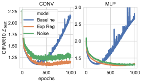

4.1 Further Experiments
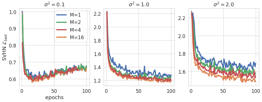
We have already ascertained that the bias implied by Theorem 4.2 has a visible impact on training performance in Figures 4 and 5. We have also already shown that the asymmetry and heavy-tails of the implicit-effect gradient noise are responsible for this performance degradation in Figure 4: models trained with Gaussian noise on gradients outperform models trained with gradient noise, and those trained with the implicit effect, on training data without batching. We corroborate these findings with experiments with mini-batching and results on test data. In Figure 7 we use the approximation of the explicit regulariser derived by Camuto et al. (2020) for computational efficiency. Convolutional networks trained with consistently outperform those trained with GNIs and mini-batching on held-out data, supporting that the implicit effect degrades performance. In Figure 8, we sample multiplicative-GNI samples and marginalise out the implicit effect as before. We model the gradients of the implicit effect, , as an distribution. Empirically, we found that when increasing the variance () of the injected noise, the gradient noise becomes increasingly heavy-tailed and skewed, i.e. decreases and increases, and in tandem larger models begin to outperform smaller models on held-out data, when trained with mini-batches. These results support that GNIs induce bias in SGD because of the asymmetric heavy-tailed noise they induce on gradient updates.
5 Conclusion
Our work lays the foundations for the study of regularisation methods from the perspective of SDEs. We have shown that Gaussian Noise Injections (GNIs), though they inject Gaussian noise in the forward pass, induce asymmetric heavy-tailed noise on gradient updates by way of the implicit effect. By modelling the overall induced noise using an asymmetric -stable noise, we demonstrate that the stationary distribution of this process gets arbitrarily distant from the so-called Gibbs measure, whose modes exactly match the local minima of the loss function, shedding light on why neural networks trained with GNIs underperform networks trained solely with the explicit effect. Given the deleterious effects of asymmetric gradient noise on gradient descent, extensions of this work could focus on methods that symmetrise gradient noise, stemming from batching or noise injections, so as to limit these negative effects.
Acknowledgements
This research was directly funded by the Alan Turing Institute under Engineering and Physical Sciences Research Council (EPSRC) grant EP/N510129/1. Alexander Camuto was supported by an EPSRC Studentship. Xiaoyu Wang and Lingjiong Zhu are partially supported by the grant NSF DMS-2053454 from the National Science Foundation. Lingjiong Zhu is also grateful to the partial support from a Simons Foundation Collaboration Grant. Mert Gürbüzbalaban’s research is supported in part by the grants Office of Naval Research Award Number N00014-21-1-2244, National Science Foundation (NSF) CCF-1814888, NSF DMS-1723085, NSF DMS-2053485. Umut Şimşekli’s research is partly supported by the French government under management of Agence Nationale de la Recherche as part of the “Investissements d’avenir” program, reference ANR-19-P3IA-0001 (PRAIRIE 3IA Institute).
References
- Agapiou et al. (2014) Agapiou, S., Stuart, A. M., and Zhang, Y. X. Bayesian posterior contraction rates for linear severely ill-posed inverse problems. Journal of Inverse and Ill-Posed Problems, 22(3):297–321, 2014.
- Bishop (1995) Bishop, C. M. Training with Noise is Equivalent to Tikhonov Regularization. Neural Computation, 7(1):108–116, 1995.
- Camuto et al. (2020) Camuto, A., Willetts, M., Şimşekli, U., Roberts, S., and Holmes, C. Explicit Regularisation in Gaussian Noise Injections. In Advances in Neural Information Processing Systems (NeurIPS), 2020.
- Cohen et al. (2019) Cohen, J., Rosenfeld, E., and Kolter, J. Z. Certified adversarial robustness via randomized smoothing. 36th International Conference on Machine Learning, ICML 2019, 2019-June:2323–2356, 2019.
- Dieng et al. (2018) Dieng, A. B., Ranganath, R., Altosaar, J., and Blei, D. M. Noisin: Unbiased regularization for recurrent neural networks. In Proceedings of the 35th International Conference on Machine Learning, pp. 1252–1261, 2018.
- Duan (2015) Duan, J. An Introduction to Stochastic Dynamics. Cambridge University Press, New York, 2015.
- Durmus & Moulines (2017) Durmus, A. and Moulines, E. Nonasymptotic convergence analysis for the unadjusted Langevin algorithm. Annals of Applied Probability, 27(3):1551–1587, 2017.
- Dybiec et al. (2007) Dybiec, B., Gudowska-Nowak, E., and Sokolov, I. Stationary states in Langevin dynamics under asymmetric Lévy noises. Physical Review E, 76(4):041122, 2007.
- Fiche et al. (2013) Fiche, A., Cexus, J. C., Martin, A., and Khenchaf, A. Features modeling with an -stable distribution: Application to pattern recognition based on continuous belief functions. Information Fusion, 14(4):504–520, 2013.
- Gao et al. (2018) Gao, X., Gürbüzbalaban, M., and Zhu, L. Global Convergence of Stochastic Gradient Hamiltonian Monte Carlo for Non-Convex Stochastic Optimization: Non-Asymptotic Performance Bounds and Momentum-Based Acceleration. arXiv:1809.04618, 2018.
- Gao et al. (2020) Gao, X., Gürbüzbalaban, M., and Zhu, L. Breaking reversibility accelerates Langevin dynamics for global non-convex optimization. In Advances in Neural Information Processing Systems (NeurIPS), 2020.
- Gnedenko & Kolmogorov (1954) Gnedenko, B. V. and Kolmogorov, A. Limit Distributions for Sums of Independent Random Variables. Addison-Wesley, Cambridge, MA, 1954. Translated by Kai Lai Chung.
- Gorenflo & Mainardi (1998) Gorenflo, R. and Mainardi, F. Random walk models for space-fractional diffusion processes. Fractional Calculus & Applied Analysis, 1:167–191, 1998.
- Gürbüzbalaban & Hu (2020) Gürbüzbalaban, M. and Hu, Y. Fractional moment-preserving initialization schemes for training fully-connected neural networks. arXiv preprint arXiv:2005.11878, 2020.
- Gürbüzbalaban et al. (2020) Gürbüzbalaban, M., Şimşekli, U., and Zhu, L. The heavy-tail phenomenon in SGD. arXiv preprint arXiv:2006.04740, 2020.
- Hodgkinson & Mahoney (2020) Hodgkinson, L. and Mahoney, M. W. Multiplicative noise and heavy tails in stochastic optimization. arXiv preprint arXiv:2006.06293, 2020.
- Imkeller & Pavlyukevich (2008) Imkeller, P. and Pavlyukevich, I. Metastable behavior of small noise Lévy-driven diffusions. ESAIM: Probability and Statistics, 12:412–437, 2008.
- Jastrzȩbski et al. (2017) Jastrzȩbski, S., Kenton, Z., Arpit, D., Ballas, N., Fischer, A., Bengio, Y., and Storkey, A. Three Factors Influencing Minima in SGD. arXiv:1711.04623, 2017.
- Kingma et al. (2015) Kingma, D. P., Salimans, T., and Welling, M. Variational dropout and the local reparameterization trick. In Advances in Neural Information Processing Systems, volume 2015-Janua, pp. 2575–2583, 2015.
- Kroneburg (2011) Kroneburg, M. The binomial coefficient for negative arguments. arXiv preprint arXiv:1105.3689, 2011.
- Kuchibhotla & Chakrabortty (2018) Kuchibhotla, A. K. and Chakrabortty, A. Moving beyond sub-Gaussianity in high dimensional statistics: Applications in covariance estimation and linear regression. arXiv:1804.02605, 2018.
- Li et al. (2017) Li, Q., Tai, C., and E, W. Stochastic modified equations and adaptive stochastic gradient algorithms. In Proceedings of the 34th International Conference on Machine Learning, pp. 2101–2110, 06–11 Aug 2017.
- Mainardi et al. (2001) Mainardi, F., Luchko, Y., and Pagnini, G. The fundamental solution of the space-time fractional diffusion equation. Fractional Calculus & Applied Analysis, 4:153–192, 2001.
- Mandt et al. (2016) Mandt, S., Hoffman, M. D., and Blei, D. M. A variational analysis of stochastic gradient algorithms. 33rd International Conference on Machine Learning, ICML 2016, 1:555–566, 2016.
- Meerschaert & Tadjeran (2004) Meerschaert, M. and Tadjeran, C. Finite difference approximation for fractional advection-dispersion flow equations. Journal of Computational and Applied Mathematics, 172:65–77, 2004.
- Nadarajah & Pogány (2016) Nadarajah, S. and Pogány, T. K. On the distribution of the product of correlated normal random variables. Comptes Rendus Mathematique, 354(2):201–204, 2016.
- Nolan (2001) Nolan, J. P. Maximum likelihood estimation and diagnostics for stable distributions. In Barndorff-Nielsen, O. E., Resnick, S. I., and Mikosch, T. (eds.), Lévy Processes: Theory and Applications, pp. 379–400. Birkhäuser Boston, Boston, MA, 2001.
- Oliveira et al. (2016) Oliveira, A., Oliveira, T. A., and Seijas-Macias, A. Skewness into the product of two normally distributed variables and the risk consequences. Revstat Statistical Journal, 14(2):119–138, 2016.
- Ortigueira (2006) Ortigueira, M. D. Riesz potential operators and inverses via fractional centred derivatives. International Journal of Mathematics and Mathematical Sciences, 2006(Article ID 48391):1–12, 2006.
- Ortiguera (2006b) Ortiguera, M. D. Fractional central differences and derivatives. IFAC Proceedings Volumes, 39(11):58–63, 2006b.
- Panloup (2008) Panloup, F. Recursive computation of the invariant measure of a stochastic differential equation driven by a Lévy process. Annals of Applied Probability, 18(2):379–426, 2008.
- Pedregosa et al. (2011) Pedregosa, F., Varoquaux, G., Gramfort, A., Michel, V., Thirion, B., Grisel, O., Blondel, M., Prettenhofer, P., Weiss, R., Dubourg, V., Vanderplas, J., Passos, A., Cournapeau, D., Brucher, M., Perrot, M., and Duchesnay, E. Scikit-learn: Machine learning in Python. Journal of Machine Learning Research, 12:2825–2830, 2011.
- Poole et al. (2014) Poole, B., Sohl-Dickstein, J., and Ganguli, S. Analyzing noise in autoencoders and deep networks. arXiv:1406.1831, 2014.
- Qian (1999) Qian, N. On the momentum term in gradient descent learning algorithms. Neural networks, 12(1):145–151, 1999.
- Raginsky et al. (2017) Raginsky, M., Rakhlin, A., and Telgarsky, M. Non-convex learning via stochastic gradient Langevin dynamics: a nonasymptotic analysis. In Conference on Learning Theory, pp. 1674–1703, 2017.
- Robbins & Monro (1951) Robbins, H. and Monro, S. A Stochastic Approximation Method. The Annals of Mathematical Statistics, 22(3):400–407, 1951.
- Roberts & Stramer (2002) Roberts, G. O. and Stramer, O. Langevin diffusions and Metropolis-Hastings algorithms. Methodology and Computing in Applied Probability, 4(4):337–357, 2002.
- Ruder (2016) Ruder, S. An overview of gradient descent optimization algorithms. arXiv:1609.04747, 2016.
- Samorodnitsky & Taqqu (1994) Samorodnitsky, G. and Taqqu, M. S. Stable Non-Gaussian Random Processes: Stochastic Models with Infinite Variance. Chapman & Hall, New York, 1994.
- Sarafrazi & Yazdi (2019) Sarafrazi, K. and Yazdi, M. Skewed alpha-stable distribution for natural texture modeling and segmentation in contourlet domain. Eurasip Journal on Image and Video Processing, 2019(1):1–12, 2019.
- Schertzer et al. (2001) Schertzer, D., Larchevêque, M., Duan, J., Yanovsky, V., and Lovejoy, S. Fractional Fokker-Planck equation for nonlinear stochastic differential equations driven by non-Gaussian Lévy stable noises. Journal of Mathematical Physics, 42(1):200–212, 2001.
- Şimşekli (2017) Şimşekli, U. Fractional Langevin Monte Carlo: Exploring Lévy driven stochastic differential equations for Markov Chain Monte Carlo. In International Conference on Machine Learning, pp. 3200–3209, 2017.
- Şimşekli et al. (2019) Şimşekli, U., Sagun, L., and Gürbüzbalaban, M. A tail-index analysis of stochastic gradient noise in deep neural networks. In Proceedings of the 36th International Conference on Machine Learning, pp. 5827–5837, 2019.
- Şimşekli et al. (2020) Şimşekli, U., Zhu, L., Teh, Y. W., and Gürbüzbalaban, M. Fractional Underdamped Langevin Dynamics: Retargeting SGD with Momentum under Heavy-Tailed Gradient Noise. In Proceedings of the 37th International Conference on Machine Learning, pp. 8970–8980, 2020.
- Şimşekli et al. (2019) Şimşekli, U., Gürbüzbalaban, M., Nguyen, T. H., Richard, G., and Sagun, L. On the Heavy-Tailed Theory of Stochastic Gradient Descent for Deep Neural Networks. arXiv:1912.00018, 2019.
- Sliusarenko et al. (2013) Sliusarenko, O. Y., Surkov, D., Gonchar, V. Y., and Chechkin, A. V. Stationary states in bistable system driven by Lévy noise. The European Physical Journal Special Topics, 216(1):133–138, 2013.
- Srivastava et al. (2014) Srivastava, N., Hinton, G., Krizhevsky, A., Sutskever, I., and Salakhutdinov, R. Dropout: A simple way to prevent neural networks from overfitting. Journal of Machine Learning Research, 15:1929–1958, 2014.
- Tian et al. (2015) Tian, W., Zhou, H., and Deng, W. A class of second order difference approximations for solving space fractional diffusion equations. Mathematics of Computation, 84(294):1703–1727, 2015.
- Vershynin (2018) Vershynin, R. High-Dimensional Probability: An Introduction with Applications in Data Science. Cambridge Series in Statistical and Probabilistic Mathematics. Cambridge University Press, 2018.
- Vladimirova et al. (2019) Vladimirova, M., Verbeek, J., Mesejo, P., and Arbel, J. Understanding priors in Bayesian neural networks at the unit level. 36th International Conference on Machine Learning, ICML 2019, 2019-June:11248–11257, 2019.
- Vladimirova et al. (2020) Vladimirova, M., Girard, S., Nguyen, H., and Arbel, J. Sub‐Weibull distributions: generalizing sub‐Gaussian and sub‐Exponential properties to heavier‐tailed distributions. Stat, 9(1):1–10, 2020.
- Webb (1994) Webb, A. R. Functional Approximation by Feed-Forward Networks: A Least-Squares Approach to Generalization. IEEE Transactions on Neural Networks, 5(3):363–371, 1994.
- Wei et al. (2020) Wei, C., Kakade, S., and Ma, T. The Implicit and Explicit Regularization Effects of Dropout. In Proceedings of the 37th International Conference on Machine Learning, pp. 10181–10192, 2020.
- Welling & Teh (2011) Welling, M. and Teh, Y. W. Bayesian Learning via Stochastic Gradient Langevin Dynamics. In Proceedings of the 28th International Conference on Machine Learning, ICML’11, pp. 681–688, Madison, WI, USA, 2011. Omnipress.
- Zhang et al. (2017) Zhang, C., Recht, B., Bengio, S., Hardt, M., and Vinyals, O. Understanding deep learning requires rethinking generalization. In 5th International Conference on Learning Representations, ICLR 2017, 2017.
- Zhang et al. (2020) Zhang, J., Karimireddy, S. P., Veit, A., Kim, S., Reddi, S., Kumar, S., and Sra, S. Why are adaptive methods good for attention models? In Advances in Neural Information Processing Systems (NeurIPS), volume 33, 2020.
- Zhou et al. (2020) Zhou, P., Feng, J., Ma, C., Xiong, C., Hoi, S., and E, W. Towards theoretically understanding why SGD generalizes better than ADAM in deep learning. In Advances in Neural Information Processing Systems (NeurIPS), volume 33, 2020.
The supplementary document is organised as follows.
-
1.
The supplementary document begins first with a presentation of additional experiments that are referenced directly in the main text (Section A).
- 2.
- 3.
- 4.
Before beginning the supplementary document we make a quick note of network architectures and training hyper-parameters.
Network Architectures
Networks were trained using stochastic gradient descent with a learning rate of 0.0003 and batch sizes specified in text. MLP network architectures are specified in text. Convolutional (CONV) networks are 2 hidden layer networks. The first layer has 32 filters, a kernel size of 4, and a stride length of 2. The second layer has 128 filters, a kernel size of 4, and a stride length of 2. The final output layer is a dense layer.
Appendix A Additional Experimental Results
Appendix B Cost Functions
B.1 Mean Square Error
In the case of regression the most commonly used loss is the mean-square error.
B.2 Cross Entropy Loss
In the case of classification, we use the cross-entropy loss. If we consider our network outputs to be the pre- of logits of the final layer then the loss is for a data-label pair
| (B.1) |
where indexes over the possible classes of the classification problem.
Appendix C Other Potential Sources of the Skewness in the Gradient Noise
The product of correlated random variables can be skewed (Oliveira et al., 2016; Nadarajah & Pogány, 2016). Our first hypothesis was that the skew came from the correlation of and . As a test, Figure C.5 of the Appendix reproduces Figure 2 with linear , isolating gradient correlation as a potential source of skew. Gradients are not skewed, demonstrating that the asymmetry stems from non-linear .
Appendix D Overview of the Assumptions
Due to space limitations and to avoid obscuring the main take home messages of our theoretical results, we did not present the two assumption required for Theorem 4.2. These two assumptions are properly presented in their respective sections (Sections E and G.6), where we first provide the required technical context for defining them in each section. In this section, we will shortly discuss the semantics of these assumptions from a higher-level perspective for the convenience of the reader.
-
•
Assumption E.1. This assumption is essentially an assumption of the tails of the function , with . In particular, in order to make our approximation scheme (to the fractional derivatives) convergent, this assumption makes sure that outside of a compact region, the function exponentially decays.
-
•
Assumption G.1. This assumption enforces a certain structure on the Euler-Maruyama discretisation given in Section 4:
As a first condition, we make sure that the step-sizes are decreasing while their sum is diverging, which is a standard assumption. The second condition is essentially a Lyapunov condition that requires the modified drift behaves well, so that we can control the weak error of the sample averages by using (Panloup, 2008). The final condition is similar to the second condition in nature, and requires ergodicity of an SDE defined through the approximate drift , in order to enable us link the weak error to the error induced by the approximation scheme used for the fractional derivatives.
Appendix E Fractional Differentiation and the Approximation Scheme
In this section, we provide the details of the Riesz-Feller type fractional derivative , whose definition was omitted in the main document for clarity. We then present the details of the approximation method for the drift term defined in (4.7).
The building block of our analysis is a first-order approximation of for any . We consider the one-dimensional case for simplicity since the Lévy motion we consider has independent coordinates, and the multi-dimensional numerical approximation can be reduced to the one-dimensional case. Assume the tail index and the skewness parameter satisfies .
When , Şimşekli (2017) developed the numerical approximation method for the drift term by approximately computing the Riesz potential333Note that when , recovers the Riesz potential. via the fractional centred difference method provided by Ortigueira (2006); Ortiguera (2006b). It is shown that for any , we have the following numerical error,
as , where is the truncation parameter and satisfies some regularity conditions, and the operator is given by
for any test function satisfying some regularity conditions, where
We study the numerical error when approximating the drift term with the skewness parameter and provide the truncation error with a truncation parameter in Corollary E.1. Based on this result, Theorem 4.2 follows, which quantifies the bias induced by -stable noise on gradient updates using the Euler-Maruyama scheme.
Instead of using the centred difference method to implement the approximation for the case, we tackle the more general case by using shifted Grünwald-Letnikov difference operators to approach the left and right fractional derivative respectively. Let us define the parameter . Then, we can now formally define the Riesz-Feller type fractional derivative operator as follows:
| (E.1) |
with
| (E.2) |
Before we proceed, we first introduce difference operators and , where and are two non-negative integers chosen to be the shifted parameters,
| (E.3) | |||
| (E.4) |
Essentially, we defined a forward shifted difference operator to approximate the left fractional derivatives, and a backward shifted difference operator to approximate the right one. The coefficients are from the coefficients of of the power series with and . For any negative fractional number and , we have
| (E.5) |
where the binomial coefficient is well-defined and the binomial series converges for any complex number ; see e.g. Kroneburg (2011). Indeed, when , we get
| (E.6) |
We first present the following first-order approximation result of the fractional derivative .
Theorem E.1.
Let denote the fractional derivative for and as in (E.1). Suppose the function . Define
| (E.7) |
Then is an approximation of with the first-order accuracy:
| (E.8) |
as , uniformly for all , where is a constant that may depend on and hides the dependence on , and .
Next, we provide an error bound for numerically computing the drift term by truncating the approximation series in Theorem E.1 as follows. Let us first define the operators and :
| (E.9) | |||
| (E.10) |
with , and .
Before we state the next result, let us first introduce the following assumption.
Assumption E.1.
Suppose the function . In addition, there exist constants satisfying
| (E.11) |
and for the constant .
We have the following result.
Corollary E.1.
Appendix F Metastability Analysis
In this section, we will focus on the metastability properties of the process
| (F.1) |
We will be interested in the first exit time, which is, roughly speaking, the expected time required for the process to exit a neighborhood of a local minimum. We will summarise the related theoretical results, which show that the first exit time behaviour of systems driven by asymmetric stable processes are similar to the ones of driven by symmetric stable processes. This informally implies that the process will quickly escape from narrow minima regions and will spend more time (in fact will get stuck) in wide minima regions. In this section, we make this argument rigorous.
For simplicity of the presentation, we consider the one-dimensional case where is an asymmetric -stable Lévy process with Lévy measure
| (F.2) |
where and and . Then, the left and right tails of the Lévy measure are given by
where , and
Let us assume that the function satisfies the following conditions:
Assumption F.1.
(i) for some ;
(ii) has exactly local minima , and local maxima , , enumerated in increasing order with and :
| (F.3) |
All extrema of are non-degenerate, i.e. , , and , .
(iii) as for some .
First, we consider the first exit time from a single well. For and , define
| (F.4) |
with the convention that and . The first exit time from the -th well is defined as
| (F.5) |
for . Let us also define
| (F.6) |
for . We have the following first exit time result from Imkeller & Pavlyukevich (2008).
Proposition F.1 (Proposition 3.1. in (Imkeller & Pavlyukevich, 2008)).
There exists such that for any , ,
| (F.7) |
where denotes the exponential distribution with mean , and
| (F.8) |
where the limit holds uniformly over .
The above result implies that as ,
| (F.9) |
If , i.e. the -th well is asymmetric and the local minimum is closer to the saddle point on the left than the saddle point on the right , then and for positive and and for negative . Similarly, if , i.e. the -th well is asymmetric and the local minimum is closer to the saddle point on the right than the saddle point on the left , then and for positive and and for negative . The intuition is that when the well is asymmetric, the dynamics can exit the well faster when there is a skewness towards the the saddle point closer to the minimum of the well.
Next, we consider transitions between the wells. For any and denote . Define
| (F.10) |
Then, we have the following result about transitions between the wells from Imkeller & Pavlyukevich (2008).
Proposition F.2 (Proposition 4.3. in (Imkeller & Pavlyukevich, 2008)).
For any and
| (F.11) |
uniformly for , , where
| (F.12) | |||
| (F.13) |
From (F.11)-(F.13), we can compute that
| (F.14) |
Therefore, is increasing in for and decreasing in for . This is consistent with the intuition that when , it is more likely for the dynamics to transit to a well on the right side, and when , it is more likely for the dynamics to transit to a well on the left side.
Next, we consider the following metastability result due to Theorem 1.1. in Imkeller & Pavlyukevich (2008). It describes the metastability phenomenon, which basically says that there exists a time scale under which the system behaves like a continuous time Markov process with a finite state space consisting of values in the set of stable attractors.
Theorem F.1 (Theorem 1.1. in (Imkeller & Pavlyukevich, 2008)).
The Markov process admits a unique invariant distribution satisfying . In the case of double well, i.e. and separated by a local maximum at , where without loss of generality we assume that , i.e. the second local minimum lies in a wider valley. A simple calculation yields that
| (F.16) |
so that it follows from and that
| (F.17) | |||
| (F.18) |
In particular, the ratio is increasing in and . That reveals that in the equilibrium the process will spend more time in the second valley if the second valley is wide and there is a drift towards to the right. In the symmetric case, i.e. , since so that in the equilibrium the process spends more time in the wider valley. In the asymmetric case, i.e. , if there is a strong skewness towards the left, i.e. and is large, then in the equilibrium the process may spend more time in the narrower valley. Indeed if and only if .
Appendix G Postponed Proofs
G.1 Proof of Lemma 3.1
Before we proceed to the proof of Lemma 3.1 we present some intermediary results that are required for the proof.
Definition G.1.
(Asymptotic order of magnitude) A positive sequence is of the same order of magnitude as another positive sequence (, i.e. ‘asymptotically equivalent’) if there exist some such that: for any .
Lemma G.1 (Lemma A.1 in (Vladimirova et al., 2019)).
Let be a normal random variable such that . Then the following asymptotic equivalence holds
We know that the centering of variables does not change their tail properties (Vershynin, 2018; Kuchibhotla & Chakrabortty, 2018). As such Lemma G.1 also applies to , as .
Lemma G.2 (Lemma 3.1 of Vladimirova et al. (2019)).
Let be a non-linearity that obeys the extended envelope property. And let be a variable for which where and denote the left and right tail of the variable respectively 444We weaken Vladimirova et al. (2019)’s requirement for to be symmetric as the proof they give still holds here.. Then we have:
| (G.1) |
Lemma G.3.
Let be variables that each obeys and .
Proof of Lemma G.3.
By Minkowski’s inequality we have that
The here are constants that upper bound the asymptotics of each norm in the sum. ∎
Proof of Lemma 3.1.
Additive Noise. Consider first the noised data, . As Lemma G.1 shows, Gaussian random variables have an norm that is asymptotically equivalent to ,
where is the dimensionality of data.
Let us now assume that , for any , for some layer . The pre-non-linearity at this layer is given by . The element of is defined as a sum,
where is the weight that maps from the neuron in layer to the in layer . By Lemma G.3,
As such if we assume the non-linearities at each layer obey the extended envelope property, then we have by Lemma G.2:
Note that . By Lemma G.3, once again , is Gaussian in its tails. By recursion, with as the base case, we have that
Multiplicative Noise. Consider first the noised data, . As Lemma G.1 shows, Gaussian random variables have an norm that is asymptotically equivalent to ,
where is the dimensionality of data.
Let us now assume that , for some layer . The pre-non-linearity at this layer is given by . The element of is defined as a sum,
where is the weight that maps from the neuron in layer to the in layer . By Lemma G.3,
As such if we assume the non-linearities at each layer obey the extended envelope property, then we have by Lemma G.2:
Note that . By Hölder’s inequality we have that,
By recursion, with as the base case, we have that
∎
G.2 Proof of Theorem 3.1
Before we proceed to the proof of Theorem 3.1 we present some intermediary results that are required for the proof.
Lemma G.4.
Let be a bounded random variable such that , then is sub-Weibull with parameter ,
| (G.2) |
Proof of Lemma G.4.
The moments of obey
Taking the root of this we find that is not dependent on and scales as a constant, . ∎
Proof of Theorem 3.1.
We first consider the gradient for a single data-label pair of the weight that maps from neuron in layer to neuron in layer . We study this gradient using the chain rule, where we decompose as
where is the (noised) activation of the neuron in the layer. Thus, the gradient noise on the weights can be described as the product of two random variables.
Additive Noise. Let us first consider the properties of for the additive case.
Regression. In the case of regression we use a mean-square-error (MSE) we have that:
where we imply all terms’ dependence on for brevity of notation. One can already see that the derivative of this object with respect to each element of will have tail properties that are asymptotically equivalent to those of , which we know by Lemma 3.1.
If we center this distribution the tail properties of this variable are unchanged (Vershynin, 2018; Kuchibhotla & Chakrabortty, 2018). In particular the asymptotic behaviour of is unchanged and we have that:
Classification. In the case of classification we use a cross-entropy (CE) error. There is no easy closed-form for here, but we can infer the properties of by studying the properties of the gradient . For CE we know that:
in the binary label case. In the multi-label classification case we typically use a , which is also a bounded function. We can already see that any noise added to will induce a change in the gradient that is inherently bounded by the non-linearity, meaning that will be bounded. As such the centered variable will also be bounded and zero mean,. By Lemma G.4 any bounded and zero mean distribution will be sub-Weibull with parameter , and will thus also be sub-Gaussian
Synthesizing the regression and classification settings we can conclude that each constitutive element of will be sub-Gaussian and will have zero mean.
We can now turn to the partial derivatives of the form . Assume is of order , with,
which entails for gradients at the previous layer we have
where
where denotes the element wise product and is the column of the weight matrix . By definition, activation functions that obey the extended envelope property will have gradients that are bounded in norm, by some constant . As such, by Lemma G.4 will be sub-Weibull with . By Hölder’s inequality we have that
where indexes over the elements of both Jacobians. By definition, we know that there exists and such that and . As such
Thus we know that the product of these two variables will be asymptotically upper-bounded by
We now need to take into account the weighted sum across rows and columns (i.e. over indices ) that occurs. By Lemma G.3 we know that
By recursion, with as the base case, gradients at layer bounded in norm by induce gradients at layer , also bounded in norm by . By recursion with the layer as the base case we can claim that,
We have now defined the first constitutive term of . Defining is much simpler:
Here , which we know is sub-Gaussian by Lemma 3.1, is once again multiplied to a bounded variable, . Thus reapplying Hölder’s inequality we obtain that
We can now bring together the characterisations of the gradients that constitute . We can re-use Hölder’s inequality to show that the product of these variables will be sub-exponential
Multiplicative Noise. In the case of multiplicative noise we know that by Lemma 3.1, the accumulated noise at layer will be of the same order as that at layer , because we are not multiplying noise to the final layer, thus
Repeating the analysis done for the additive case we can claim that,
We have now defined the first constitutive term of . We now define .
Here , which we know is sub-Weibull with a parameter by Lemma 3.1, is once again multiplied to a bounded variable, . Thus reapplying Hölder’s inequality we obtain that
We can re-use Hölder’s inequality to show that the product of these variables will be sub-Weibull with
Mean of Noise. Finally, by definition these gradients are zero mean,
∎
G.3 Proof of Theorem 4.1
Before we proceed to the proof of Theorem 4.1, we present some technical results that will be used in the proof of Theorem 4.1 later.
For the -dimensional asymmetric fractional Langevin dynamics , its infinitesimal generator is given in the following proposition.
Proposition G.1.
The asymmetric fractional Langevin dynamics has the infinitesimal generator:
| (G.3) |
where
| (G.4) |
where is the -th basis vector in , i.e. a -dimensional unit vector with -th coordinate being and all the other coordinates being .
Proof of Proposition G.1.
Since the asymmetric fractional Langevin dynamics is driven by the -dimensional , it suffices to show that the infinitesimal generator of -dimensional is given by
| (G.5) |
We start the proof by considering the dimension first. The one-dimensional -stable Lévy motion with tail-index and skewness has the infinitesimal generator given by:
| (G.6) |
where is chosen so that to be consistent with in for any . Thus, we can compute that
| (G.7) |
which yields that
| (G.8) |
Therefore, with ,
| (G.9) |
where
| (G.10) |
Similarly, for the multi-dimensional case, we can show that the infinitesimal generator for is given by:
| (G.11) |
where
| (G.12) |
where is the -th basis vector in , i.e. a -dimensional unit vector with -th coordinate being and all the other coordinates being . ∎
We recall that for any , , and , we have
| (G.13) |
where
| (G.14) |
and
| (G.15) |
In the next result, we provide an alternative formula for that is defined in (4.7).
Proposition G.2.
For any , , and , we have
| (G.16) |
with .
Proof of Proposition G.2.
Let us first consider the case when , . We have
| (G.17) |
where
| (G.18) | |||
| (G.19) |
Similarly, when , , and , we have
| (G.20) |
where
| (G.21) |
∎
Now, we are ready to prove Theorem 4.1.
Proof of Theorem 4.1.
We recall from Proposition G.1 that the asymmetric fractional Langevin dynamics has the infinitesimal generator:
| (G.22) |
where is given in (G.4).
It follows that the adjoint operator of is given by:
| (G.23) |
The probability density function of the Lévy-driven SDE satisfies the Fokker-Planck equation (Schertzer et al., 2001):
| (G.24) |
We can compute that
Hence, we conclude that is an invariant distribution of the asymmetric fractional Langevin dynamics (4.6). Finally, if is Lipschitz continuous in , then is the unique invariant distribution of (4.6), see e.g. Schertzer et al. (2001). ∎
G.4 Proof of Theorem E.1
Theorem E.1 provides a first-order approximation of the fractional derivative when .
Based on the work of Meerschaert & Tadjeran (2004), we will show a first-order approximation for the asymmetric fractional derivative when by using the shifted Grünwald-Letnikov difference operators defined in (E.3) and (E.4). Before we proceed to the proof of Theorem E.1, we will first present the Fourier transform property from equations (1) and (12) in Tian et al. (2015).
Property G.1 ((Tian et al., 2015)).
Let and . The Fourier transform of and satisfy the following identities:
| (G.25) |
where denotes the Fourier transform of , such that
Now, we are ready to prove Theorem E.1.
Proof of Theorem E.1.
The main idea for the proof of Theorem E.1 is to use the Fourier transform to estimate the difference between and , and then apply the inverse Fourier transform to complete the proof. By the linearity of Fourier transforms, we can apply Fourier transform to (E.3) to obtain
| (G.26) |
Similarly, we can compute that
| (G.27) |
In addition, since and are analytic for any complex number , there exist series expansions so that by the first-order Taylor expansion we have
| (G.28) |
Next, define a function as the difference between and . By the linearity of Fourier transform, we have
| (G.29) |
where we used the fact that for any real , , we have so that which implies equality (a), and we applied Euler’s formula with to get equality (b). By our assumption , we have
for a constant that may depend on . Hence, by taking a sufficiently small , we obtain,
where we also used the inequality that for , and is a constant may depend on . When , the inverse Fourier transform exists with , i.e. , and it follows that
| (G.30) |
where hides the dependence on , and , and is a constant that may depend on .
Hence, we conclude that
| (G.31) |
The proof is complete. ∎
G.5 Proof of Corollary E.1
With the definitions of the truncated series defined in (E.9) and in (E.10), we are now ready to prove Corollary E.1.
Proof of Corollary E.1.
We will first control the difference . Then the triangular inequality can be applied with the fractional derivative approximation error bound in Theorem E.1 to get the numerical truncation error.
By using the definitions of and , under the Assumption E.1, there exist two universal constants and so that
| (G.32) |
Next, by applying Stirling’s formula, we have as :
Therefore, it follows from (G.32) that
| (G.33) |
where we abused the notation such that , in (G.33) may differ from , in (G.32). Finally, the triangular inequality yields that
where and are two universal constants following Assumption E.1. The proof is completed. ∎
G.6 Proof of Theorem 4.2
First, let us recall that is the sample average, where satisfies the Euler-Maruyama discretisation with the approximated drift :
| (G.34) |
The corresponding SDE of (G.34) is given as
| (G.35) |
and we define , where is the stationary distribution of (G.35).
Next, let us introduce the following assumption that is needed for Theorem 4.2.
Assumption G.1.
(i) Assume that the step sizes are decreasing and the sum diverges such that .
(ii) Let be a function in , if , with some constant and is bounded. Then there exists , and , such that and with defined in (4.7). And the statement also holds for .
Before we proceed to the proof of Theorem 4.2, let us state a technical lemma bounding the error of , where and follow SDEs in (4.6) and (G.35).
Lemma G.5.
Proof.
The proof is inspired by the proof of Lemma 3 in Şimşekli (2017). Let and be the corresponding Markov semigroups, i.e. Using the Markov semigroup property, following Lemma 3 in Şimşekli (2017), we have
where and are the linear generators of and , such that, for , . The infinitesimal generators and are computed in (G.22). By the interchangeability of integration and differentiation, we have
By the ergodicity assumptions, for a bounded function , there exist some constants and so that
| (G.37) |
Using the boundedness assumption for and Corollary E.1, and the fact that , we have
| (G.38) |
where the constants , and may depend on and the bound for . ∎
Now we are ready to prove Theorem 4.2.