Euclidean Affine Functions and Applications to Calendar Algorithms

Abstract

We study properties of Euclidean affine functions (EAFs), namely those of the form $f(r)=(\alpha\cdot r+\beta)/\delta$, and their closely related expression $\mathring{f}(r)=(\alpha\cdot r+\beta)\%\delta$, where $r$, $\alpha$, $\beta$ and $\delta$ are integers, and where $/$ and $\%$ respectively denote the quotient and remainder of Euclidean division. We derive algebraic relations and numerical approximations that are important for the efficient evaluation of these expressions in modern CPUs. Since simple division and remainder are particular cases of EAFs (when $\alpha=1$ and $\beta=0$), the optimisations proposed in this paper can also be appplied to them. Such expressions appear in some of the most common tasks in any computer system, such as printing numbers, times and dates. We use calendar calculations as the main application example because it is richer with respect to the number of EAFs employed. Specifically, the main application presented in this article relates to Gregorian calendar algorithms. We will show how they can be implemented substantially more efficiently than is currently the case in widely used C, C++, C# and Java open source libraries. Gains in speed of a factor of two or more are common.

Keywords: Euclidean Affine Functions, Integer Division, Calendar Algorithms

Mathematics Subject Classification (2020): 65Y04, 68R01

1 Introduction

Divisions by constants appear in some of the most common tasks performed by software systems, including printing decimal numbers (division by powers of $10$) and working with times (division by $24$, $60$ and $3600$). Since division is the slowest of the four basic arithmetical operations, various authors [1, 5, 10, 16, 22] have proposed strength reduction optimisations (i.e., the replacement of instructions with alternatives that are mathematically equivalent but faster) for integer divisions when divisors are constants known by the compiler. The algorithms proposed by Granlund and Montgomery [10] have been implemented by major compilers.

A typical example that will appear later in this article is the division

$$n/1461=2\ \!939\ \!745\cdot n/2^{32},\quad\forall n\in[0,28\ \!825\ \!529[.$$

The problem involves finding, for the given divisor $1461$, the multiplier 2 ​939 ​745, the exponent $32$, and the boundary $28\ \!825\ \!529$ of the interval in which equality holds. Clearly, there are many possible solutions.

Remainder calculation is a closely related problem, also arising in the tasks mentioned above, although the cited works do not consider optimisations for this operation. Compilers are content to apply strength reduction to obtain the quotient $r/\delta$ and the remainder evaluating $r-\delta\cdot(r/\delta)$. For this reason, [13, 23] considered the problem of directly obtaining the remainder without first calculating the quotient.

This paper expands previous works in two ways. Firstly, it considers the more general setting of Euclidean affine functions (EAFs) $f(r)=(\alpha\cdot r+\beta)/\delta$ where $\alpha$, $\beta$ and $\delta$ are integer constants and $r$ is an integer variable. Secondly, it suggests optimisations that are even more effective in applications where both the quotient and the remainder need to be evaluated.

We derive EAF-related equalities that provide alternative ways of evaluating expressions commonly used in applications. (For instance, $r-\delta\cdot(r/\delta)$, which is used to obtain the remainder as explained above.) These equalities underpin optimisations, other than strength reduction, that take into account aspects of modern CPUs. Specifically, they foster instruction-level parallelism implemented by superscalar processors and they profit from the backward compatibility features that drove the design of the x86_64 instruction set.

Calendar calculations are a rich application field for our EAF results. Performed by various software systems, they tackle questions such as: What is the date today? For how many days do interest rates accrue over the period of a loan? Your mobile phone no doubt performed a similar calculation while you read this paragraph.

Our algorithms are substantially faster than those in widely used open source implementations, as shown by benchmarks against counterparts in glibc [7, 8] (Linux contains a similar implementation [14]), Boost [4], libc++ [15], .NET [17] and OpenJDK [19] (Android contains the same implementations [2]). Our algorithms are also faster than others found in the academic literature [3, 6, 11, 12, 20, 21].

The critical point setting apart implementations of calendar algorithms is how they deal with non-linearities caused by irregular month and year lengths. Some authors [14, 8, 17] resort to look-up tables, which can be costly when the L1-level cache is cold. They conduct linear searches on these tables, entailing branching that can cause stalls in the processor’s execution pipeline. Others [3, 6, 11, 12, 4, 15, 20, 21] tackle the issue entirely through EAFs. Nevertheless, they do not go far enough and do not use the mathematical properties derived in this paper. To the best of our knowledge, the most successful attempt at achieving this efficiency is Baum [3]. This author provides some explanations, but appears to resort to trial and error when it comes to pre-calculating certain magic numbers used in his algorithm. We go further by providing a systematic and general framework for such calculations.

Our paper and its main contributions are organised as follows.

Section 2 introduces EAFs and derives some of their properties. Although they are common in applications, we were unable to find any systematic coverage of them. Hatcher [11] and Richards [21] appear to be aware of some of the results of Theorem 2.5, but they do not point to any proof.

Section 3 concerns efficient evaluations of EAFs. Theorems 3.2 and 3.4 generalise prior-known results on division to EAFs. Section 3.1 revisits those results and brings geometric insights to the problem. Theorem 3.11 concerns the efficient evaluation of residuals: they are to EAFs what remainders are to division. The optimisation proposed by Theorem 3.11 is fundamentally different from other optimisations, both in the present paper and in prior works, since it does not involve strength reduction. Indeed, this theorem shows how to break a data dependency present in the instructions currently emitted by compilers, enabling instruction-level parallelism, as we shall see in Example 3.12.

Section 4 provides a generic mathematical framework for calendars, which we use to study the Gregorian calendar. Efficient algorithms for this calendar are derived in Sections 5 and 6. Section 7 presents performance analysis.

We finish this introduction by setting the notation used throughout and recalling some well-known results.

On the totally ordered Euclidean domain of integer numbers $(\mathbb{Z},+,\cdot,\leq)$, forward slash $/$ and percent $\%$ respectively denote the quotient and remainder of Euclidean division. More precisely, given $n,\delta\in\mathbb{Z}$ with $\delta\neq 0$, there exist unique $q,r\in\mathbb{Z}$, with $0\leq r<|\delta|$, such that $n=q\cdot\delta+r$. Then $n/\delta=q$ and $n\%\delta=r$. (These concepts, for non-negative operands, match the usual operators / and % of many programming languages in the C-family.)

We follow the usual algebraic order of operation rules and, in accordance with C-style languages, we give $\%$ the same precedence as $\cdot$ and $/$. Hence, $a\cdot b\%c=(a\cdot b)\%c$, $a\%b\cdot c=(a\%b)\cdot c$ and $a/b\%c=(a/b)\%c$, $a\%b/c=(a\%b)/c$. Moreover, $a+b\%c=a+(b\%c)$, and $a-b\%c=a-(b\%c)$. In general, $a\cdot b/c\neq a\cdot(b/c)$ and $(a+b)/c\neq a/c+b/c$. This indicates that these precedence rules are even more important than when working in algebraic fields. Nevertheless, we shall drop unnecessary parentheses henceforth.

The set of non-negative integer numbers is denoted by $\mathbb{Z^{+}}=\{x\in\mathbb{Z}\ ;\ x\geq 0\}$.

On the totally ordered field of rational numbers $(\mathbb{Q},+,\cdot,\leq)$, the reciprocal of $\delta\in\mathbb{Q}\setminus\{0\}$ is denoted by $\delta^{-1}$. For $n$, $\delta\in\mathbb{Z}$ with $\delta\neq 0$, we shall write $n\cdot\delta^{-1}\in\mathbb{Q}$ to distinguish it from $n/\delta\in\mathbb{Z}$. If the former belongs to $\mathbb{Z}$, then $n\cdot\delta^{-1}=n/\delta$. This distinction is particularly important when dealing with inequalities. On the one hand, for $x,y,\delta\in\mathbb{Z}$ with $\delta>0$, we have $x\cdot\delta^{-1}\geq y\cdot\delta^{-1}$ if, and only if, $x\geq y$; and on the another hand $x/\delta\geq y/\delta$ if $x\geq y$, but the converse does not hold.

For any $x\in\mathbb{Q}$, there exist unique $\left\lfloor x\right\rfloor\in\mathbb{Z}$ and $\left\lceil x\right\rceil\in\mathbb{Z}$ such that $\left\lfloor x\right\rfloor\leq x<\left\lfloor x\right\rfloor+1$ and $\left\lceil x\right\rceil-1<x\leq\left\lceil x\right\rceil$. For any finite set $X$, the number of elements of $X$ is denoted by $\#X$.

2 Euclidean affine functions

Multiplication by $60$ converts hours to minutes. Conversely, division by $60$ converts minutes to hours. If the amount of minutes in an hour were variable, these problems would be more complex. Since months and years have variable numbers of days, such complexities arise in calendar calculations. Different ways of tackling this problem appear across implementations with various degrees of performance. Nevertheless, similarities between calendar calculations and the previous linear problems are stronger than they might appear, as revealed by our study of EAFs.

Definition 2.1.

A function $f:\mathbb{Z}\rightarrow\mathbb{Z}$ is a Euclidean affine function, EAF for short, if it has the form $f(r)=(\alpha\cdot r+\beta)/\delta$ for all $r\in\mathbb{Z}$ and fixed $\alpha$, $\beta$, $\delta\in\mathbb{Z}$ with $\delta\neq 0$.

This terminology is ours. The analogues of EAFs in higher dimensions appear in Discrete Geometry and are called quasi-affine transformations. That area focuses on periodicity, tiling and other geometric aspects, whereas we are concerned with efficient calculations. We therefore use the term EAF to distinguish between these two approaches.

Definition 2.2.

Let $f$ be the EAF $f(r)=(\alpha\cdot r+\beta)/\delta$. The residual function of $f$ is $\mathring{f}(r)=(\alpha\cdot r+\beta)\%\delta$ or, equivalently, $\mathring{f}(r)=\alpha\cdot r+\beta-\delta\cdot f(r)$.

An important function related to $f(r)=r/\delta$ is its right inverse $\hat{f}(q)=\delta\cdot q$. If $\delta>0$ and $r\in[\hat{f}(q),\hat{f}(q+1)[\ =[\delta\cdot q,\delta\cdot(q+1)[$, then $f(r)=q$ and $\mathring{f}(r)=r-\delta\cdot(r/\delta)=r-\hat{f}(f(r))=r-\hat{f}(q)$. As we shall see, Theorem 2.5 generalises these results and supports the following terminology.

Definition 2.3.

Let $f$ be the EAF $f(r)=(\alpha\cdot r+\beta)/\delta$, with $\delta\geq\alpha>0$. The minimal right inverse of $f$ is the EAF $\hat{f}(q)=(\delta\cdot q+\alpha-\beta-1)/\alpha$.

Lemma 2.4.

Let $f$ be the EAF $f(r)=(\alpha\cdot r+\beta)/\delta$, with $\delta>0$, and $g:\mathbb{Z}\rightarrow\mathbb{Z}$. For any $q\in\mathbb{Z}$ such that $f(g(q)-1)<f(g(q))$, we have:

$$r\in\mathbb{Z}\quad\text{and}\quad f(r)=f(g(q))\quad\Longrightarrow\quad\mathring{f}(r)/\alpha=r-g(q).$$

Proof.

Since $\mathring{f}(r)=\alpha\cdot r+\beta-\delta\cdot f(r)$, we have $\mathring{f}(g(q))=\alpha\cdot g(q)+\beta-\delta\cdot f(g(q))$. Hence,

$$\mathring{f}(r) =\alpha\cdot r+\beta-\delta\cdot f(r)=\alpha\cdot(r-g(q))+\alpha\cdot g(q)+\beta-\delta\cdot f(g(q))$$

$$=\alpha\cdot(r-g(q))+\mathring{f}(g(q)).$$

We will show that $0\leq\mathring{f}(g(q))<\alpha$ and it will follow that $\mathring{f}(r)/\alpha=r-g(q)$. By definition of $\mathring{f}$ and $\%$ we obtain $\mathring{f}(g(q))\geq 0$. Suppose, by contradiction, that $\mathring{f}(g(q))\geq\alpha$. Then,

$$\alpha\cdot(g(q)-1)+\beta =\alpha\cdot g(q)+\beta-\alpha=\delta\cdot f(g(q))+\mathring{f}(g(q))-\alpha$$

$$\geq\delta\cdot f(g(q)).$$

Dividing the above by $\delta$ gives $f(g(q)-1)\geq f(g(q))$, which contradicts the assumption on $q$. ∎

Theorem 2.5.

Let $f$ be the EAF $f(r)=(\alpha\cdot r+\beta)/\delta$ with $\delta\geq\alpha>0$. Then, for any $r$ and $q\in\mathbb{Z}$ we have:

1. $f(\hat{f}(q))=q$ and $f(\hat{f}(q)-1)=q-1$;

2. $f(r)=q$ if, and only if, $r\in[\hat{f}(q),\hat{f}(q+1)[$;

3. $r\in[\hat{f}(f(r)),\hat{f}(f(r)+1)[$ and $\mathring{f}(r)/\alpha=r-\hat{f}(f(r))$.

Proof.

Let $q\in\mathbb{Z}$ and set $n=\delta\cdot q+\alpha-\beta-1$ so that $\hat{f}(q)=(\delta\cdot q+\alpha-\beta-1)/\alpha=n/\alpha$.

(i): Since $0\leq n\%\alpha\leq\alpha-1$ and $\alpha\leq\delta$, we have:

$$0\leq\alpha-1-n\%\alpha\leq\delta-1-n\%\alpha<\delta.$$ (1)

From $\hat{f}(q)=n/\alpha$, we obtain $\alpha\cdot\hat{f}(q)=n-n\%\alpha$ and

$$\alpha\cdot\hat{f}(q)+\beta=n+\beta-n\%\alpha=\delta\cdot q+\alpha-1-n\%\alpha.$$

This and Equation 1 yield $(\alpha\cdot\hat{f}(q)+\beta)/\delta=q$, that is, $f(\hat{f}(q))=q$. Furthermore, the equality above gives:

$$\alpha\cdot(\hat{f}(q)-1)+\beta=\delta\cdot q-1-n\%\alpha=\delta\cdot(q-1)+\delta-1-n\%\alpha.$$

This and Equation 1 yield $(\alpha\cdot(\hat{f}(q)-1)+\beta)/\delta=q-1$, that is, $f(\hat{f}(q)-1)=q-1$.

(ii): Since $\delta\geq\alpha>0$, $f$ is non-decreasing. If $r\leq\hat{f}(q)-1$, then $f(r)\leq f(\hat{f}(q)-1)=q-1$. If $\hat{f}(q)\leq r\leq\hat{f}(q+1)-1$, then $q=f(\hat{f}(q))\leq f(r)\leq f(\hat{f}(q+1)-1)=q$ (the last equality follows from (i) applied to $q+1$) and thus, $f(r)=q$. Finally, if $r\geq\hat{f}(q+1)$, then $f(r)\geq f(\hat{f}(q+1))=q+1$ (again from (i) applied to $q+1$).

(iii): Since $\delta\geq\alpha>0$, $\hat{f}$ is strictly increasing and there thus exists $p\in\mathbb{Z}$ such that $r\in[\hat{f}(p),\hat{f}(p+1)[$. Using (i) and (ii) (for $q=p$) gives $f(\hat{f}(p))=p$, $f(\hat{f}(p)-1)=p-1$ and $f(r)=p$. In particular, $f(\hat{f}(p)-1)<f(\hat{f}(p))$ and $f(r)=f(\hat{f}(p))$. Lemma 2.4 (for $g=\hat{f}$ and $q=p$) therefore gives $\mathring{f}(r)/\alpha=r-\hat{f}(p)$. Using $p=f(r)$ again yields $r\in[\hat{f}(f(r)),\hat{f}(f(r)+1)[$ and $\mathring{f}(r)/\alpha=r-\hat{f}(f(r))$. ∎

From (i), $\hat{f}$ is a right inverse of $f$. Item (ii) goes further, showing the minimum solution $r$ for the equation $f(r)=q$ is $r=\hat{f}(q)$, hence the wording of Definition 2.3.

Example 2.6.

Theorem 2.5 for $f(r_{0})=(4\cdot r_{0}+3)/146097$ and $\hat{f}(q)=146097\cdot q/4$ gives:

$$r_{0}\in[\hat{f}(q),\hat{f}(q+1)[\quad\Longrightarrow\quad(4\cdot r_{0}+3)/146097=q\quad\text{and}\quad(4\cdot r_{0}+3)\%146097/4=r_{0}-\hat{f}(q).$$

Each side of last equality provides a way to evaluate the same quantity. To analyse performance trade-offs, we introduce auxiliary variables referring to partial results and compare both methods side-by-side:

$$\begin{aligned} &\text{ Calculation of }(4\cdot r_{0}+3)\%146097/4:\\ n&=4\cdot r_{0}+3,\\ q&=n/146097,\\ u&=n-146097\cdot q,\quad(\text{\em i.e., }u=n\%146097)\\ r&=u/4,\\ \end{aligned}\qquad\vrule\qquad\begin{aligned} &\text{ Calculation of }r_{0}-\hat{f}(q):\\ n&=4\cdot r_{0}+3,\\ q&=n/146097,\\ v&=146097\cdot q/4\quad(\text{\em i.e., }v=\hat{f}(q)),\\ r&=r_{0}-v.\end{aligned}$$

For fairness of comparison, $u$ is set to $n-146097\cdot q$ rather than $n\%146097$, since the former better represents the CPU instructions typically emitted by compilers to evaluate the latter. Both listings show exactly the same operations, the only difference being the order of the last two operations. Our preference for the left listing will be explained in the next steps of the Gregorian calendar algorithm. Indeed, the expressions above appear in these calculations and are followed by the evaluation of $4\cdot r+3$. If $r$ is calculated as shown on the left, then $4\cdot r+3=4\cdot(u/4)+3$ and smart compilers reduce this expression to $u\ |\ 3$, where $|$ denotes bitwise or.

Example 2.7.

Theorem 2.5 for $f(r_{1})=(4\cdot r_{1}+3)/1461$ and $\hat{f}(q)=1461\cdot q/4$ gives:

$$r_{1}\in[\hat{f}(q),\hat{f}(q+1)[\quad\Longrightarrow\quad(4\cdot r_{1}+3)/1461=q\quad\text{and}\quad(4\cdot r_{1}+3)\%1461/4=r_{1}-\hat{f}(q).$$

Example 2.8.

Theorem 2.5 for $f(r_{2})=(5\cdot r_{2}+461)/153$ and $\hat{f}(m_{0})=(153\cdot m_{0}-457)/5$ gives:

$$r_{2}\in[\hat{f}(m_{0}),\hat{f}(m_{0}+1)[\quad\Longrightarrow\quad(5\cdot r_{2}+461)/153=m_{0}\quad\text{and}\quad(5\cdot r_{2}+461)\%153/5=r_{2}-\hat{f}(m_{0}).$$

3 Fast evaluation of Euclidean affine functions

This section covers optimisations for $(\alpha\cdot r+\beta)/\delta$. The particular case $\alpha=1$ and $\beta=0$ has been considered by many authors [1, 5, 10, 16, 22], who have derived strength reductions whereby $r/\delta$ is reduced to a multiplication and cheaper operations. Major compilers implement the algorithms of [10]. Faster algorithms exist but compilers are not able to use them. For instance, $r$ might be restricted to a small interval but, unaware of this fact, the compiler must assume that $r$ can take any allowed value for its type, usually in an interval of form $[0,2^{w}[$. We change focus and instead of looking for an algorithm on a given interval, we start with the best algorithm we know and search the largest interval on which it can be applied. If such an interval is satisfactory for our application, then we use this algorithm.

When $\delta$ is a power of two, the evaluation of $r/\delta$ reduces to a bitwise shift, which is very cheap in binary CPUs. The Fundamental Theorem of Arithmetic implies that $\delta$ is a power of two if, and only if, $2^{k}\%\delta=0$ for some $k\in\mathbb{Z^{+}}$. For $(\alpha\cdot r+\beta)/\delta$, a trivial reduction is also available when $2^{k}\cdot\alpha\%\delta=0$. Indeed, we have $2^{k}\cdot\alpha=\delta\cdot(2^{k}\cdot\alpha/\delta)$, and setting $\alpha^{\prime}=2^{k}\cdot\alpha/\delta$ and $\beta^{\prime}=2^{k}\cdot\beta/\delta$ gives $2^{k}\cdot\alpha=\delta\cdot\alpha^{\prime}$ and

$$(\alpha\cdot r+\beta)/\delta=\left(2^{k}\cdot\alpha\cdot r+2^{k}\cdot\beta\right)/\left(2^{k}\cdot\delta\right)=\left(\delta\cdot\alpha^{\prime}\cdot r+2^{k}\cdot\beta\right)/\left(2^{k}\cdot\delta\right)=\left(\alpha^{\prime}\cdot r+\beta^{\prime}\right)/2^{k}.$$

Conceptually, to evaluate $(\alpha\cdot r+\beta)/\delta$ we multiply $r$ by $\alpha\cdot\delta^{-1}$ and add the result to $\beta\cdot\delta^{-1}$. Assume, for the time being, that $\beta=0$. We take an approximation $\alpha^{\prime}\in\mathbb{Z}$ of $2^{k}\cdot\alpha\cdot\delta^{-1}$, where $k\in\mathbb{Z^{+}}$ is carefully chosen, and evaluate $\alpha^{\prime}\cdot r/2^{k}$. Two natural choices for $\alpha^{\prime}$ are $\left\lceil 2^{k}\cdot\alpha\cdot\delta^{-1}\right\rceil$ and $\left\lfloor 2^{k}\cdot\alpha\cdot\delta^{-1}\right\rfloor$, covered by Theorems 3.2 and 3.4, respectively.

Lemma 3.1.

Let $f$ be the EAF $f(r)=(\alpha\cdot r+\beta)/\delta$. Then,

$$\alpha\cdot(r/\delta)=f(r)-f(r\%\delta),\qquad\forall r\in\mathbb{Z}.$$

Proof.

$f(r)=(\alpha\cdot(\delta\cdot(r/\delta)+r\%\delta)+\beta)/\delta=\alpha\cdot(r/\delta)+(\alpha\cdot(r\%\delta)+\beta)/\delta=\alpha\cdot(r/\delta)+f(r\%\delta)$. ∎

The next theorem does not assume $2^{k}\cdot\alpha\%\delta\neq 0$, but when equality holds a simpler reduction can be made as seen above. The result becomes more interesting when we do have $2^{k}\cdot\alpha\%\delta\neq 0$, in which case $\left\lceil 2^{k}\cdot\alpha\cdot\delta^{-1}\right\rceil=2^{k}\cdot\alpha/\delta+1$.

Theorem 3.2.

Let $k\in\mathbb{Z^{+}}$ and $f$ be the EAF $f(r)=(\alpha\cdot r+\beta)/\delta$ with $\delta>0$. Set $\alpha^{\prime}=2^{k}\cdot\alpha/\delta+1$, $\varepsilon=\delta-2^{k}\cdot\alpha\%\delta$ and $\beta^{\prime}=-\min\{\alpha^{\prime}\cdot r-2^{k}\cdot f(r)\ ;\ r\in[0,\delta[\ \}$. For $r\in[0,\delta[$ define:

$$q(r)=\min\{p\in\mathbb{Z^{+}}\ ;\ \varepsilon\cdot p+\alpha^{\prime}\cdot r+\beta^{\prime}-2^{k}\cdot f(r)\geq 2^{k}\}\quad\text{and}\quad M(r)=\delta\cdot q(r)+r.\\$$

Let $N=\min\{M(r)\ ;\ r\in[0,\delta[\ \}$. Then,

$$(\alpha\cdot r+\beta)/\delta=\left(\alpha^{\prime}\cdot r+\beta^{\prime}\right)/2^{k},\quad\forall r\in[0,N[.$$

Proof.

First note that $q(r)$ is well-defined since $\varepsilon>0$. So are $M(r)$ and $N$. Also, $\delta>0$ implies $M(r)\geq 0$ and, consequently, $N\geq 0$. Nevertheless, we do not exclude the possibility that $N=0$, in which case this theorem’s conclusion is vacuously true. The sequel assumes that $N>0$ and $r\in\mathbb{Z}$. Note that:

$$\varepsilon=\delta-\left(2^{k}\cdot\alpha-\delta\cdot\left(2^{k}\cdot\alpha/\delta\right)\right)=\delta\cdot\left(1+2^{k}\cdot\alpha/\delta\right)-2^{k}\cdot\alpha=\delta\cdot\alpha^{\prime}-2^{k}\cdot\alpha.$$ (2)

It follows that $\delta\cdot\alpha^{\prime}\cdot(r/\delta)-2^{k}\cdot\alpha\cdot(r/\delta)=\varepsilon\cdot(r/\delta)$. Hence,

$$\alpha^{\prime}\cdot r-2^{k}\cdot\alpha\cdot(r/\delta)=\alpha^{\prime}\cdot(\delta\cdot(r/\delta)+r\%\delta)-2^{k}\cdot\alpha\cdot(r/\delta)=\varepsilon\cdot(r/\delta)+\alpha^{\prime}\cdot(r\%\delta).$$

From the above and Lemma 3.1 we conclude that:

$$\alpha^{\prime}\cdot r-2^{k}\cdot f(r)=\varepsilon\cdot(r/\delta)+\alpha^{\prime}\cdot(r\%\delta)-2^{k}\cdot f(r\%\delta).$$ (3)

Suppose further that $r\in[0,N[$. By definition, $N\leq M(r\%\delta)$ and hence $r<M(r\%\delta)$, i.e., $\delta\cdot(r/\delta)+r\%\delta<\delta\cdot q(r\%\delta)+r\%\delta$. It follows that $r/\delta<q(r\%\delta)$. From the definition of $q(r\%\delta)$ and the fact that $r/\delta\geq 0$, we obtain:

$$\varepsilon\cdot(r/\delta)+\alpha^{\prime}\cdot(r\%\delta)+\beta^{\prime}-2^{k}\cdot f(r\%\delta)<2^{k}.$$ (4)

The definition of $\beta^{\prime}$ yields $\alpha^{\prime}\cdot(r\%\delta)+\beta^{\prime}-2^{k}\cdot f(r\%\delta)\geq 0$. This and $\varepsilon\cdot(r/\delta)\geq 0$ mean that the left side of Equation 4 is non-negative. Therefore, Equation 3 yields $0\leq\alpha^{\prime}\cdot r+\beta^{\prime}-2^{k}\cdot f(r)<2^{k}$ and the conclusion follows from Euclidean division by $2^{k}$. ∎

Example 3.3.

Theorem 3.2 for $k=5$ and $f(m_{0})=(153\cdot m_{0}-457)/5$ yields $\alpha^{\prime}=980$, $\beta^{\prime}=-2928$ and $N=12$, that is,

$$(153\cdot m_{0}-457)/5=(980\cdot m_{0}-2928)/2^{5},\quad\forall m_{0}\in[0,12[.$$

The next theorem does assume that $2^{k}\cdot\alpha\%\delta\neq 0$ and thus, $2^{k}\cdot\alpha/\delta=\left\lfloor 2^{k}\cdot\alpha\cdot\delta^{-1}\right\rfloor$.

Theorem 3.4.

Let $k\in\mathbb{Z^{+}}$ and $f$ be the EAF $f(r)=(\alpha\cdot r+\beta)/\delta$ with $\delta>0$ and $2^{k}\cdot\alpha\%\delta>0$. Set $\alpha^{\prime}=2^{k}\cdot\alpha/\delta$, $\varepsilon=2^{k}\cdot\alpha\%\delta$ and $\beta^{\prime}=\min\{2^{k}-1-(\alpha^{\prime}\cdot r-2^{k}\cdot f(r))\ ;\ r\in[0,\delta[\ \}$. For $r\in[0,\delta[$ define:

$$q(r)=\min\{p\in\mathbb{Z^{+}}\ ;\ -\varepsilon\cdot p+\alpha^{\prime}\cdot r+\beta^{\prime}-2^{k}\cdot f(r)<0\}\quad\text{and}\quad M(r)=\delta\cdot q(r)+r.\\$$

Let $N=\min\{M(r)\ ;\ r\in[0,\delta[\ \}$. Then,

$$(\alpha\cdot r+\beta)/\delta=(\alpha^{\prime}\cdot r+\beta^{\prime})/2^{k},\quad\forall r\in[0,N[.$$

Proof.

The assumption $2^{k}\cdot\alpha\%\delta>0$ means that $\varepsilon>0$ and ensures that $q(r)$ is well-defined, as are $M(r)$ and $N$. Also, $\delta>0$ implies $M(r)\geq 0$ and, consequently, $N\geq 0$. Nevertheless, we do not exclude the possibility that $N=0$, in which case this theorem’s conclusion is vacuously true. The sequel assumes that $N>0$ and $r\in\mathbb{Z}$.

Note that:

$$\varepsilon=2^{k}\cdot\alpha\%\delta=2^{k}\cdot\alpha-\delta\cdot\left(2^{k}\cdot\alpha/\delta\right)=2^{k}\cdot\alpha-\delta\cdot\alpha^{\prime}.$$ (5)

It follows that $2^{k}\cdot\alpha\cdot(r/\delta)-\delta\cdot\alpha^{\prime}\cdot(r/\delta)=\varepsilon\cdot(r/\delta)$. Hence,

$$\alpha^{\prime}\cdot r-2^{k}\cdot\alpha\cdot(r/\delta)=\alpha^{\prime}\cdot(\delta\cdot(r/\delta)+r\%\delta)-2^{k}\cdot\alpha\cdot(r/\delta)=-\varepsilon\cdot(r/\delta)+\alpha^{\prime}\cdot(r\%\delta).$$

From the above and Lemma 3.1 we conclude that:

$$\alpha^{\prime}\cdot r-2^{k}\cdot f(r)=-\varepsilon\cdot(r/\delta)+\alpha^{\prime}\cdot(r\%\delta)-2^{k}\cdot f(r\%\delta).$$ (6)

Suppose further that $r\in[0,N[$. By definition $N\leq M(r\%\delta)$ and hence, $r<M(n\%\delta)$, i.e., $\delta\cdot(r/\delta)+r\%\delta<\delta\cdot q(r\%\delta)+r\%\delta$. Therefore, $r/\delta<q(r\%\delta)$. From the definition of $q(r\%\delta)$ and the fact that $r/\delta\geq 0$, we obtain:

$$-\varepsilon\cdot(r/\delta)+\alpha^{\prime}\cdot(r\%\delta)+\beta^{\prime}-2^{k}\cdot f(r\%\delta)\geq 0.$$ (7)

The definition of $\beta^{\prime}$ yields $\alpha^{\prime}\cdot(r\%\delta)+\beta^{\prime}-2^{k}\cdot f(r\%\delta)\leq 2^{k}-1<2^{k}$. This and $\varepsilon\cdot(r/\delta)\geq 0$ mean that the left side of Equation 7 is less than $2^{k}$. Therefore, Equation 6 yields $0\leq\alpha^{\prime}\cdot r+\beta^{\prime}-2^{k}\cdot f(r)<2^{k}$ and the conclusion follows from Euclidean division by $2^{k}$. ∎

Example 3.5.

Theorem 3.4 for $k=5$ and $f(m_{0})=(153\cdot m_{0}-457)/5$ yields $\alpha^{\prime}=979$, $\beta^{\prime}=-2919$ and $N=34$, namely:

$$(153\cdot m_{0}-457)/5=(979\cdot m_{0}-2919)/2^{5},\quad\forall m_{0}\in[0,34[.$$ (8)

Examples 3.3 and 3.5 give two fast alternatives for the same EAF. In this case, the latter has the advantage of being valid on a larger range, $[0,34[$ as opposed to $[0,12[$, but in other cases the opposite is true. For EAFs known prior to compilation, one can find both alternatives and select the one that is valid in the larger range. Compilers can do the same for EAFs found in source code. However, if the costs of finding the two alternatives need to be avoided, then a simple and fast-selecting criterion is based on the following heuristics. To maximise $N$ we seek to maximise $q(r)$, which is the minimum value of $p$ for which $\varepsilon\cdot p$ reaches a certain threshold. The smaller $\varepsilon$ is, the larger $p$ must be for this to happen. Hence, we choose the alternative with the smallest $\varepsilon$ amongst its two possible values, namely, $\varepsilon_{1}=\delta-2^{k}\cdot\alpha\%\delta$ and $\varepsilon_{2}=2^{k}\cdot\alpha\%\delta$. (If $\delta$ is odd, then $\varepsilon_{1}\neq\varepsilon_{2}$.) Another interpretation of this criterion is that it sets $\alpha^{\prime}$ to the best approximation of $2^{k}\cdot\alpha\cdot\delta^{-1}$ given by $\left\lceil 2^{k}\cdot\alpha\cdot\delta^{-1}\right\rceil$ or $\left\lfloor 2^{k}\cdot\alpha\cdot\delta^{-1}\right\rfloor$. Indeed, if $2^{k}\cdot\alpha\%\delta\neq 0$, then Equations 2 and 5 give:

$$\varepsilon_{1} =\delta\cdot\left(2^{k}\cdot\alpha/\delta+1\right)-2^{k}\cdot\alpha =\delta\cdot\left\lceil 2^{k}\cdot\alpha\cdot\delta^{-1}\right\rceil-2^{k}\cdot\alpha,$$

$$\varepsilon_{2} =2^{k}\cdot\alpha-\delta\cdot\left(2^{k}\cdot\alpha/\delta\right) =2^{k}\cdot\alpha-\delta\cdot\left\lfloor 2^{k}\cdot\alpha\cdot\delta^{-1}\right\rfloor.$$

It follows that $\varepsilon_{1}<\varepsilon_{2}$ if, and only if, $\left\lceil 2^{k}\cdot\alpha\cdot\delta^{-1}\right\rceil-2^{k}\cdot\alpha\cdot\delta^{-1}<2^{k}\cdot\alpha\cdot\delta^{-1}-\left\lfloor 2^{k}\cdot\alpha\cdot\delta^{-1}\right\rfloor$.

Example 3.6.

Theorem 3.4 for $k=16$ and $f(r_{2})=(5\cdot r_{2}+461)/153$ yields $\alpha^{\prime}=2141$, $\beta^{\prime}=197913$ and $N=734$, namely:

$$(5\cdot r_{2}+461)/153=(2141\cdot r_{2}+197913)/2^{16},\quad\forall r_{2}\in[0,734[.$$ (9)

In Theorems 3.2 and 3.4, $\alpha^{\prime}$ and $\varepsilon$ are obtained in $O(1)$ operations and $\beta^{\prime}$ is found by an $O(\delta)$ search. For each $r\in[0,\delta[$, $q(r)$ and $N(r)$ are calculated in $O(1)$ operations. $N$ and the overall search for a fast EAF then have $O(\delta)$ time complexity. Since many EAFs featuring in calendar calculations have small divisors, finding more efficient alternatives for them is reasonably fast.

3.1 Fast division – the special case $\alpha=1,\beta=0$

This section examines $r/\delta$ with $\delta>0$, i.e., the particular case of the EAF $f(r)=(\alpha\cdot r+\beta)/\delta$ where $\alpha=1$, $\beta=0$ and $\delta>0$.

For $\alpha=1$, Theorems 3.2 and 3.4 set $\alpha^{\prime}$ to $\left\lceil 2^{k}\cdot\delta^{-1}\right\rceil$ and $\left\lfloor 2^{k}\cdot\delta^{-1}\right\rfloor$, respectively. The former is the choice taken by [1, 5, 10] and the latter by [16]. Finally, [22] and an appendix to [5], consider both and, in this particular case, rigourously justify the heuristics we have suggested for choosing between the two approaches.

This section follows a more direct path but most of its results can be obtained from the above for $\alpha=1$ and $\beta=0$. For instance, for $\alpha^{\prime}>0$, let $\beta^{\prime}=-\min\{\alpha^{\prime}\cdot r-2^{k}\cdot f(r)\ ;\ r\in[0,\delta[\ \}$ as in Theorem 3.2. Since $f(r)=r/\delta=0$ for $r\in[0,\delta[$, we have $\beta^{\prime}=-\min\{\alpha^{\prime}\cdot r\ ;\ r\in[0,\delta[\ \}=0$. Hence, in contrast to the general case, there is no need for an $O(\delta)$ search to obtain $\beta^{\prime}$. Similarly, $\beta^{\prime}=\min\{2^{k}-1-(\alpha^{\prime}\cdot r-2^{k}\cdot f(r))\ ;\ r\in[0,\delta[\ \}$, as defined by Theorem 3.4, can be proven to be $\alpha^{\prime}+(2^{k}\%\delta-1)$, the same value found in [16]. Theorem 3.4 assumes that $2^{k}\%\delta\geq 1$ and, in the definition of $\beta^{\prime}$, had we subtracted $2^{k}\%\delta$ instead of $1$ the proof would still work but $\beta^{\prime}$ would have a smaller value, namely, $\beta^{\prime}=\alpha^{\prime}$. In this case, the final reduction would be $r/\delta=\alpha^{\prime}\cdot(r+1)/2^{k}$ as found in [5, 22]. In addition, by making $\beta^{\prime}$ smaller, $q(r)$, $M(r)$ and $N$ also decrease. Hence, Theorem 3.4 obtains a range of validity that is no smaller than the one obtained in [5, 22].

The remainder of this section focuses on the round-up approach but the round-down alternative could be similarly considered. Our reasons for this are that the round-up approach is mostly used by compilers and that the appearance of the term $r+1$ can potentially lead to an overflow.

Lemma 3.7.

Let $\delta,k\in\mathbb{Z^{+}}$ with $\delta>0$. Set $\alpha^{\prime}=2^{k}/\delta+1$ and $\varepsilon=\delta-2^{k}\%\delta$. Then, $\alpha^{\prime}\cdot\delta=2^{k}+\varepsilon$ and for any $n\in\mathbb{Z}$ we have:

$$\alpha^{\prime}\cdot n/2^{k}=n/\delta\quad\text{if, and only if,}\quad 0\leq\varepsilon\cdot(n/\delta)+\alpha^{\prime}\cdot(n\%\delta)<2^{k}.$$ (10)

Proof.

Taking $\alpha=1$ in Theorem 3.2 gives the same $\alpha^{\prime}$ and $\varepsilon$ as here. Equation 2 then reads $\varepsilon=\alpha^{\prime}\cdot\delta-2^{k}$. Similarly, from Equation 3 with $f(n)=n/\delta$ and $f(n\%\delta)=n\%\delta/\delta=0$ we obtain:

$$\alpha^{\prime}\cdot n-2^{k}\cdot(n/\delta)=\varepsilon\cdot(n/\delta)+\alpha^{\prime}\cdot(n\%\delta).$$

The result follows from Euclidean division by $2^{k}$. ∎

Since $\alpha^{\prime},\varepsilon\in\mathbb{Z^{+}}$, we have $0\leq\varepsilon\cdot(n/\delta)+\alpha^{\prime}\cdot(n\%\delta)$ for all $n\in\mathbb{Z^{+}}$. There is an illuminating geometric interpretation for the second part of the double inequality in Equation 10 that follows from mapping each $n\in\mathbb{Z^{+}}$ to $P_{n}=(n/\delta,n\%\delta)$ in the $xy$ plane. Figure 1 shows, for $\delta=5$, some points of particular interest labelled by their circled value. Notably, the origin $P_{0}=(0/5,0\%5)$, $P_{1}=(1/5,1\%5)$ and $P_{5}=(5/5,5\%5)$. Inequality $\varepsilon\cdot(n/\delta)+\alpha^{\prime}\cdot(n\%\delta)<2^{k}$ states that $P_{n}$ is below the line $\varepsilon\cdot x+\alpha^{\prime}\cdot y=2^{k}$, which is represented by the dotted line in Figure 1, for $k=8$, $\varepsilon=4$ and $\alpha^{\prime}=52$. Hence, Equation 10 means that a point below the line corresponds to $n\in\mathbb{Z^{+}}$ such that $n/\delta=\alpha^{\prime}\cdot n/2^{k}$ and a point above or on the line is related to $n$ such that $n/\delta\neq\alpha^{\prime}\cdot n/2^{k}$.

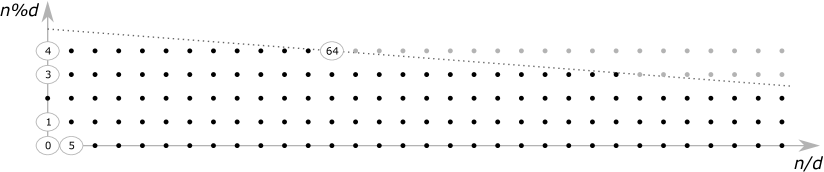
Figure 1: The geometry of replacing $n/\delta$ with $\alpha^{\prime}\cdot n/2^{k}$, where $\delta=5$ and $k=8$, $\alpha^{\prime}=2^{k}/\delta+1=52$.

If the slope of the dotted line is not too steep (more precisely, $-\varepsilon\cdot\alpha^{\prime-1}\geq-1)$, then the graph makes it obvious that the smallest $N$ for which $P_{N}$ is above or on the dotted line must lie on the line $y=\delta-1=4$. In our case $N=64$. For Theorem 3.2, with $\alpha=1$ and $\beta=0$, this means that $N=M(\delta-1)$. In particular, we are not interested in either $M(r)$ or $q(r)$ when $r\neq\delta-1$. This and $\beta^{\prime}=0$ turn finding a fast EAF and its interval of applicability $[0,N[$ into an $O(1)$ calculation rather than an $O(\delta)$ search as in the general case. These geometric ideas are present although algebraically disguised in the proof of Theorem 3.8.

The result of Theorem 3.8 also appears in [5]. In addition to providing the aforementioned geometric insights and an arguably simpler proof, we favour faster algorithms over range of applicability. In other words, we reduce division to multiplication and bitwise shift and find the largest $N$ for which this optimisation yields correct results for all dividends in $[0,N[$. (In [5] $N$ is called critical value and is denoted by $N_{cr}$.)

Theorem 3.8.

Let $\delta,k\in\mathbb{Z^{+}}$ with $\delta>0$. Set $\alpha^{\prime}=2^{k}/\delta+1$, $\varepsilon=\delta-2^{k}\%\delta$ and $N=\left\lceil\alpha^{\prime}\cdot\varepsilon^{-1}\right\rceil\cdot\delta-1$. If $\varepsilon\leq\alpha^{\prime}$, then:

$$n/\delta=\alpha^{\prime}\cdot n/2^{k},\quad\forall n\in[0,N[.$$

Proof.

Let $N^{\prime}=N-\delta=\left(\left\lceil\alpha^{\prime}\cdot\varepsilon^{-1}\right\rceil-2\right)\cdot\delta+\delta-1$. We have $N^{\prime}/\delta=\left\lceil\alpha^{\prime}\cdot\varepsilon^{-1}\right\rceil-2$ and $N^{\prime}\%\delta=\delta-1$. Recall from Lemma 3.7 that $\alpha^{\prime}\cdot\delta-\varepsilon=2^{k}$. Therefore, using $\varepsilon\cdot\left\lceil\alpha^{\prime}\cdot\varepsilon^{-1}\right\rceil<\alpha^{\prime}+\varepsilon$ we obtain:

$$\varepsilon\cdot(N^{\prime}/\delta)+\alpha^{\prime}\cdot(N^{\prime}\%\delta)=\varepsilon\cdot\left\lceil\alpha^{\prime}\cdot\varepsilon^{-1}\right\rceil-2\cdot\varepsilon+\alpha^{\prime}\cdot\delta-\alpha^{\prime}<2^{k}.$$ (11)

Let $n\in\mathbb{Z^{+}}$ with $n<N$. We shall show that $0\leq\varepsilon\cdot(n/\delta)+\alpha^{\prime}\cdot(n\%\delta)<2^{k}$ and the result will follow from Lemma 3.7. Since $\varepsilon$, $\alpha^{\prime}$ and $r$ are non-negative, it is sufficient to show that $\varepsilon\cdot(n/\delta)+\alpha^{\prime}\cdot(n\%\delta)<2^{k}$.

Assume first that $n\leq N^{\prime}$. As a result, $n/\delta\leq N^{\prime}/\delta$. Then use Equation 11 to obtain:

$$\varepsilon\cdot(n/\delta)+\alpha^{\prime}\cdot(n\%\delta)\leq\varepsilon\cdot(N^{\prime}/\delta)+\alpha^{\prime}\cdot(\delta-1)=\varepsilon\cdot(N^{\prime}/\delta)+\alpha^{\prime}\cdot(N^{\prime}\%\delta)<2^{k}.$$

Now assume that $N^{\prime}+1\leq n<N$. Then $\left(\left\lceil\alpha^{\prime}\cdot\varepsilon^{-1}\right\rceil-1\right)\cdot\delta\leq n<\left(\left\lceil\alpha^{\prime}\cdot\varepsilon^{-1}\right\rceil-1\right)\cdot\delta+\delta-1$. Hence, $n/\delta=\left\lceil\alpha^{\prime}\cdot\varepsilon^{-1}\right\rceil-1=N^{\prime}/\delta+1=N/\delta$. Since $n<N$, we must have $n\%\delta\leq N\%\delta-1=\delta-2$. Therefore,

$$\varepsilon\cdot(n/\delta)+\alpha^{\prime}\cdot(n\%\delta) \leq\varepsilon\cdot(N^{\prime}/\delta+1)+\alpha^{\prime}\cdot(\delta-2)=\varepsilon\cdot(N^{\prime}/\delta)+\alpha^{\prime}\cdot(\delta-1)+\varepsilon-\alpha^{\prime}$$

$$\leq\varepsilon\cdot(N^{\prime}/\delta)+\alpha^{\prime}\cdot(N^{\prime}\%\delta).$$

The result follows from Equation 11. ∎

Remark 3.9.

If $\delta$ is not a power of two and $2^{k}\geq\delta\cdot(\delta-2)$, then $\varepsilon\leq\alpha^{\prime}$. Indeed, under these hypotheses we have $2^{k}/\delta\geq\delta-2$ and $2^{k}\%\delta\geq 1$. It follows that $\delta-2^{k}\%\delta\leq\delta-1\leq 2^{k}/\delta+1$, i.e., $\varepsilon\leq\alpha^{\prime}$.

Example 3.10.

Consider the division $n_{2}/1461$. For $k=39$ the constants given by Theorem 3.8 are $\alpha^{\prime}=376\ \!287\ \!347$, $\varepsilon=79$ and $N=6\ \!958\ \!934\ \!390$. Since $\varepsilon\leq\alpha^{\prime}$, this theorem gives:

$$n_{2}/1461=376\ \!287\ \!347\cdot n_{2}/2^{39},\quad\forall n_{2}\in[0,6\ \!958\ \!934\ \!390[.$$ (12)

Following [10], major compilers replace the expression on the left with the one on the right when $n_{2}$ is a 32-bit unsigned integer. (It is worth mentioning that $k=39$ is the smallest value for which $N\geq 2^{32}$.)

For $k=32$, the constants given by Theorem 3.8 are $\alpha^{\prime}=2\ \!939\ \!745$, $\varepsilon=149$ and $N=28\ \!825\ \!529$. Hence,

$$n_{2}/1461=2\ \!939\ \!745\cdot n_{2}/2^{32},\quad\forall n_{2}\in[0,28\ \!825\ \!529[.$$ (13)

Although the interval is smaller than the one for $k=39$, it is large enough for the Gregorian calendar algorithm that we present later on. Example 3.12 will unveil the advantage of Equation 13 over Equation 12.

3.2 Fast evaluation of residual functions

Theorems 3.2 and 3.4 suggest optimisations for EAFs, generalising the current practice for divisions revisited by Theorem 3.8. Our next result extends the optimisation to residual functions.

Theorem 3.11.

Let $f$ and $f^{\prime}$ be EAFs given by $f(r)=(\alpha\cdot r+\beta)/\delta$ and $f^{\prime}(r)=(\alpha^{\prime}\cdot r+\beta^{\prime})/\delta^{\prime}$, with $\delta\geq\alpha>0$, and assume that $f\equiv f^{\prime}$ on $[a,b[$. If $a=\hat{f}(f(a))$ and $f^{\prime}(a-1)<f^{\prime}(a)$, then:

$$\mathring{f}(r)/\alpha=\mathring{f^{\prime}}(r)/\alpha^{\prime}\quad\forall r\in[a,b[.$$

Proof.

Let $r\in[a,b[$ and set $q=f(r)$. From Theorem 2.5-(iii), we obtain $\mathring{f}(r)/\alpha=r-\hat{f}(q)$. We will finish the proof by using Lemma 2.4 to show that $\mathring{f^{\prime}}(r)/\alpha^{\prime}=r-\hat{f}(q)$.

Since $\delta\geq\alpha>0$, both $f$ and $\hat{f}$ are non-decreasing. Hence, from $a\leq r\leq b-1$ we obtain $\hat{f}(f(a))\leq\hat{f}(f(r))\leq\hat{f}(f(b-1))$. By assumption, $a=\hat{f}(f(a))$ and Theorem 2.5-(iii) (for $r=b-1$) gives $b-1\in[\hat{f}(f(b-1)),\hat{f}(f(b-1)+1)[$, in particular $\hat{f}(f(b-1))\leq b-1$. Therefore, $a\leq\hat{f}(f(r))\leq b-1$, in other words, $\hat{f}(q)\in[a,b[$.

Since $f\equiv f^{\prime}$ in $[a,b[$ and $\hat{f}(q)$ is in this interval, we have $f^{\prime}(\hat{f}(q))=f(\hat{f}(q))$. Theorem 2.5-(i) yields $f(\hat{f}(q))=q$ and thus $f^{\prime}(\hat{f}(q))=q=f(r)$.

Similarly, it can be shown that if $\hat{f}(q)-1\in[a,b[$, then $f^{\prime}(\hat{f}(q)-1)=q-1$, specifically, $f^{\prime}(\hat{f}(q)-1)<f^{\prime}(\hat{f}(q))$. On the other hand, if $\hat{f}(q)-1\notin[a,b[$, then we must have $\hat{f}(q)=a$ and the assumption on $f^{\prime}$ also gives $f^{\prime}(\hat{f}(q)-1)<f^{\prime}(\hat{f}(q))$.

We have shown that $f^{\prime}(\hat{f}(q)-1)<f^{\prime}(\hat{f}(q))$ and $f(r)=f^{\prime}(\hat{f}(q))$. Then, Lemma 2.4 applied to $f^{\prime}$ (instead of $f$) and $g=\hat{f}$ gives $\mathring{f^{\prime}}(r)/\alpha^{\prime}=r-\hat{f}(q)$. ∎

Example 3.12.

Consider the EAFs $f(n_{2})=n_{2}/1461$, $\hat{f}(q)=q\cdot 1461$ and $f^{\prime}(n_{2})=2\ \!939\ \!745\cdot n_{2}/2^{32}$. Equation 13 shows that $f(n_{2})=f^{\prime}(n_{2})$ for all $n_{2}\in[a,b[\ =[0,28\ \!825\ \!529[$. Simple calculations give $\hat{f}(f(0))=0$ and $f^{\prime}(-1)=-1<0=f^{\prime}(0)$. Hence, it follows from Equations 13 and 3.11 that:

$$n_{2}/1461=2\ \!939\ \!745\cdot n_{2}/2^{32}\quad\text{and}\quad n_{2}\%1461=2\ \!939\ \!745\cdot n_{2}\%2^{32}/2\ \!939\ \!745,\quad\forall n_{2}\in[0,28\ \!825\ \!529[.$$

Revisiting Example 2.7 we show three alternatives that can be used to obtain $q_{2}=(4\cdot r_{1}+3)/1461$ and $r_{2}=r_{1}-1461\cdot q_{2}/4$ side-by-side. The first evaluates $r_{2}$ as expressed. The second uses the expression $(4\cdot r_{1}+3)\%1461/4$ seen in Example 2.7. The third is similar but replaces $n_{2}/1461$ and $n_{2}\%1461$ with the aforementioned alternatives.

$$\begin{aligned} n_{2}&=4\cdot r_{1}+3,\\ \\ q_{2}&=n_{2}/1461,\\ r_{2}&=r_{1}-1461\cdot q_{2}/4,\\ \end{aligned}\quad\vrule\quad\begin{aligned} n_{2}&=4\cdot r_{1}+3,\\ \\ q_{2}&=n_{2}/1461,\\ r_{2}&=(n_{2}-1461\cdot q_{2})/4,\ (\text{\em i.e., }r_{2}=n_{2}\%1461/4)\\ \end{aligned}\quad\vrule\quad\begin{aligned} n_{2}&=4\cdot r_{1}+3,\\ u_{2}&=2\ \!939\ \!745\cdot n_{2},\\ q_{2}&=u_{2}/2^{32},\\ r_{2}&=u_{2}\%2^{32}/2\ \!939\ \!745/4.\\ \end{aligned}$$

We are interested in instructions emitted by compilers for the three listings above but, for clarity, we did not perform typical compiler optimisations (e.g., substituting division by $4$ and $2^{32}$ with bitwise shifts). However, in the middle listing we did substitute $n_{2}\%1461$ with $n_{2}-1461\cdot q_{2}$ for greater resemblance to emitted instructions and fairer comparison with the first listing. Compilers reduce division by $1461$ to multiplication and bitwise shift, the same operations used to get $u_{2}$ and $q_{2}$ in the third listing. Therefore, up to and including the calculation of $q_{2}$, the instructions for the three columns are the same and only the constants differ.

The calculation of $r_{2}$ in the first two listings requires three instructions: one multiplication, one subtraction and one bitwise shift $(/4$). For the third listing, there appear to be four: one bitwise and ($\%2^{32}$), one multiplication and one bitwise shift (compilers’ reduction of $/2\ \!939\ \!745$), and another bitwise shift ($/4$). In fact, these two bitwise shifts collapse into one. Hence, there are also three instructions for the third listing. We conclude that the number of instructions is exactly the same for the three listings, but this is only part of the story. The breakthrough of the third listing is removing the dependency of $r_{2}$ on $q_{2}$, seen in the first two listings, which forces the CPU to wait for the calculation of $q_{2}$ to finish before starting that of $r_{2}$. In listing three, once $u_{2}$ is obtained, the evaluations of $q_{2}$ and $r_{2}$ can start concurrently. There is a small but worthwhile price to pay for this parallelisation and even that can be avoided in some platforms as we shall see now.

The calculations of $q_{2}$ and $r_{2}$ need $u_{2}$ to be stored in two different registers, which implies a mov from the register on which $u_{2}$ was originally obtained. This does not necessarily increase the number of instructions because instead of leaving the compiler to reduce division by $1461$ to multiplication and a bitwise shift of $39$ bits (see Equation 12), we perform our own reduction (see Equation 13) using $32$ bits. For backward compatibility, x86-64 CPUs provide mov instructions that reset the upper $32$ bits of $64$ registers, effectively performing a mov and a bitwise and at the same time. Hence, the operation $\%2^{32}$ in the calculation of $r_{2}$ might come for free.

Example 3.13.

Consider the EAFs $f(r_{2})=(5\cdot r_{2}+461)/153$, $\hat{f}(m_{0})=(153\cdot m_{0}-457)/5$, and $f^{\prime}(r_{2})=(2141\cdot r_{2}+197913)/2^{16}$. Equation 9 states that $f(r_{2})=f^{\prime}(r_{2})$ for all $r_{2}\in[a,b[\ =[0,734[$. Simple calculations give $\hat{f}(f(0))=0$ and $f^{\prime}(-1)=2<3=f^{\prime}(0)$. It follows from Equations 9 and 3.11 that:

$$(5\cdot r_{2}+461)/153 =(2141\cdot r_{2}+197913)/2^{16}\quad\text{and}$$

$$(5\cdot r_{2}+461)\%153/5 =(2141\cdot r_{2}+197913)\%2^{16}/2141,\quad\forall r_{2}\in[0,734[.$$

Example 2.8 shows that the left side of the last equation matches $d_{0}=r_{2}-(153\cdot m_{0}-457)/5$. Hence, as in Example 3.12, we have three alternatives for evaluating this quantity. The analysis of Example 3.12 also holds here and once $n_{3}=2141\cdot r_{2}+197913$ is obtained the calculations of $m_{0}=n_{3}/2^{16}$ and $d_{0}=n_{3}\%2^{16}/2141$ can start concurrently. Furthermore, in some platforms, the operation $\%2^{16}$ might come for free.

Example 3.14.

In line with the previous examples, we have

$$n/3600 =1\ \!193\ \!047\cdot n/2^{32}, n\%3600 =1\ \!193\ \!047\cdot n\%2^{32}/1\ \!193\ \!047, \forall n \in[0,2\ \!257\ \!199[;$$

$$n/60 =71\ \!582\ \!789\cdot n/2^{32}, n\%60 =71\ \!582\ \!789\cdot n\%2^{32}/71\ \!582\ \!789, \forall n \in[0,97\ \!612\ \!919[;$$

$$n/10 =429\ \!496\ \!730\cdot n/2^{32}, n\%10 =429\ \!496\ \!730\cdot n\%2^{32}/429\ \!496\ \!730, \forall n \in[0,1\ \!073\ \!741\ \!829[.$$

Compilers create a data dependency when evaluating the left side of the equalities above but not when the expressions on the right are used. The first two lines can be used in conversions of the seconds elapsed since the start of the day, a quantity in $[0,86400[$, to hours, minutes and seconds. The third line can be used in conversions of non-negative integers up to $9$ digits into their decimal representations.

3.3 Quick remainder – the special case $\alpha=1$, $\beta=0$

Again for this particular case, the EAF $f(n)=(\alpha\cdot n+\beta)/\delta$ simplifies to $f(n)=n/\delta$ and its residual function simplifies to $\mathring{f}(n)=n\%\delta$. In this section we use Theorem 3.8 and Theorem 3.11 to derive an efficient way to calculate remainders.

Formally, Theorem 3.8 states how to replace $n/\delta$ with $\alpha^{\prime}\cdot n/2^{k}$, where $\alpha^{\prime}\approx 2^{k}\cdot\delta^{-1}$ and $k\in\mathbb{Z^{+}}$. Theorem 3.11 then gives the equality $n\%\delta=(\alpha^{\prime}\cdot n\%2^{k})/\alpha^{\prime}$ and Theorem 3.8, again, suggests replacing division by $\alpha^{\prime}$ with multiplication by an approximation of $2^{k}\cdot\alpha^{\prime-1}$ and division by $2^{k}$. It turns out that $\delta\approx 2^{k}\cdot\alpha^{\prime-1}$ is the approximation we need and we obtain $n\%\delta=\delta\cdot(\alpha^{\prime}\cdot n\%2^{k})/2^{k}$. This is the idea behind our next theorem.

Theorem 3.15.

Let $\delta,k\in\mathbb{Z^{+}}$ with $\delta>0$. Set $\alpha^{\prime}=2^{k}/\delta+1$, $\varepsilon=\delta-2^{k}\%\delta$ and $M=\left\lceil 2^{k}\cdot\varepsilon^{-1}\right\rceil$. If $\varepsilon\leq\alpha^{\prime}$, then:

$$n\%\delta=\delta\cdot(\alpha^{\prime}\cdot n\%2^{k})/2^{k},\quad\forall n\in[0,M[.$$ (14)

Proof.

Set $N=\left\lceil\alpha^{\prime}\cdot\varepsilon^{-1}\right\rceil\cdot\delta-1\geq\alpha^{\prime}\cdot\varepsilon^{-1}\cdot\delta-1$. Recall from Lemma 3.7 that $\alpha^{\prime}\cdot\delta=2^{k}+\varepsilon$ and thus $N\geq(2^{k}+\varepsilon)\cdot\varepsilon^{-1}-1=2^{k}\cdot\varepsilon^{-1}$. It follows that $N\geq M$. Theorem 3.8 gives:

$$n/\delta=\alpha^{\prime}\cdot n/2^{k},\quad\forall n\in[0,N[.$$ (15)

Hence, for the EAFs $f(n)=n/\delta$ and $f^{\prime}(n)=\alpha^{\prime}\cdot n/2^{k}$, Equation 15 states that $f\equiv f^{\prime}$ on $[0,N[$. Simple calculations give $\hat{f}(f(0))=\delta\cdot f(0)=0$ and $f^{\prime}(-1)<f^{\prime}(0)$. Theorem 3.11 (for $\alpha=1$ and $[a,b[\ =[0,N[$) therefore yields:

$$n\%\delta=(\alpha^{\prime}\cdot n\%2^{k})/\alpha^{\prime},\quad\forall n\in[0,N[.$$ (16)

Let $n\in[0,M[$ and set $m=\varepsilon\cdot(n/\delta)+\alpha^{\prime}\cdot(n\%\delta)$. Since $n<N$, we have $n/\delta\leq N/\delta=\left\lceil\alpha^{\prime}\cdot\varepsilon^{-1}\right\rceil-1<\alpha^{\prime}\cdot\varepsilon^{-1}$. It follows that $0\leq\varepsilon\cdot(n/\delta)<\alpha^{\prime}$. Hence, $m/\alpha^{\prime}=n\%\delta$ and $m\%\alpha^{\prime}=\varepsilon\cdot(n/\delta)$. Moreover, Equations 15 and 3.7 give $0\leq m<2^{k}$. Since $\alpha^{\prime}\cdot n=\alpha^{\prime}\cdot(\delta\cdot(n/\delta)+n\%\delta)=2^{k}\cdot(n/\delta)+\varepsilon\cdot(n/\delta)+\alpha^{\prime}\cdot(n\%\delta)=2^{k}\cdot(n/\delta)+m$, we conclude that $\alpha^{\prime}\cdot n\%2^{k}=m$.

Since $n<M$, we have $\varepsilon\cdot n<2^{k}$, otherwise $n\geq 2^{k}\cdot\varepsilon^{-1}$ and then, $n\geq M$. Therefore:

$$0\leq\varepsilon\cdot(m/\alpha^{\prime})+\delta\cdot(m\%\alpha^{\prime})=\varepsilon\cdot(n\%\delta)+\delta\cdot\varepsilon\cdot(n/\delta)=\varepsilon\cdot n<2^{k}.$$ (17)

Using $\alpha^{\prime}\cdot\delta=2^{k}+\varepsilon$ again gives $2^{k}=\delta\cdot\alpha^{\prime}-\varepsilon=(\delta-1)\cdot\alpha^{\prime}+\alpha^{\prime}-\varepsilon$ and, since $0\leq\alpha^{\prime}-\varepsilon<\alpha^{\prime}$, we obtain $2^{k}/\alpha^{\prime}=\delta-1$ and $2^{k}\%\alpha^{\prime}=\alpha^{\prime}-\varepsilon$, that is, $\delta=2^{k}/\alpha^{\prime}+1$ and $\varepsilon=\alpha^{\prime}-2^{k}\%\alpha^{\prime}$. Therefore, Equation 17 and Lemma 3.7 (with $\alpha^{\prime}$ and $\delta$ interchanged) give $m/\alpha^{\prime}=\delta\cdot m/2^{k}$, namely, $(\alpha^{\prime}\cdot n\%2^{k})/\alpha^{\prime}=\delta\cdot(\alpha^{\prime}\cdot n\%2^{k})/2^{k}$.

Finally, Equation 16 yields $n\%\delta=(\alpha^{\prime}\cdot n\%2^{k})/\alpha^{\prime}=\delta\cdot(\alpha^{\prime}\cdot n\%2^{k})/2^{k}$. ∎

Example 3.16.

Revisiting Example 3.14, Theorem 3.15 gives

$$n\%3600 =3600\cdot(1\ \!193\ \!047\cdot n\%2^{32})/2^{32}, \forall n \in[0,2\ \!255\ \!761[;$$

$$n\%60 =60\cdot(71\ \!582\ \!789\cdot n\%2^{32})/2^{32}, \forall n \in[0,97\ \!612\ \!894[;$$

$$n\%10 =10\cdot(429\ \!496\ \!730\cdot n\%2^{32})/2^{32}, \forall n \in[0,1\ \!073\ \!741\ \!824[.$$

The expressions on the right side of the equals sign provide efficient ways of evaluating remainders. However, greater benefits are achieved when they are used in conjunction with the quotient expressions presented in Example 3.14.

The equality in Equation 14 also appears in [13]. As in other works, it focuses on obtaining the value $k\in\mathbb{Z^{+}}$ for which the equality holds on an interval of the form $[0,2^{w}[$ or, in other words, $2^{w}\leq M$ as the next result shows.

Corollary 3.17.

Let $\delta,l,w\in\mathbb{Z^{+}}$ with $0<\delta<2^{w}$ and $\delta-2^{w+l}\%\delta\leq 2^{l}$. Set $\alpha^{\prime}=2^{w+l}/\delta+1$. Then,

$$n\%\delta=\delta\cdot(\alpha^{\prime}\cdot n\%2^{w+l})/2^{w+l},\quad\forall n\in[0,2^{w}[.$$

Proof.

Set $k=w+l$, $\varepsilon=\delta-2^{k}\%\delta$ and $M=\left\lceil 2^{k}\cdot\varepsilon^{-1}\right\rceil$. From Theorem 3.15, it is sufficient to show that $\varepsilon\leq\alpha^{\prime}$ and $2^{k}\leq M$. Since $\delta<2^{w}$ and $\varepsilon\leq 2^{l}$, we have $\delta\cdot\varepsilon<2^{w+l}=2^{k}$ and thus, $\varepsilon\leq 2^{k}/\delta<\alpha^{\prime}$. We also have $M\geq 2^{k}\cdot\varepsilon^{-1}\geq 2^{k}\cdot 2^{-l}=2^{w}$. ∎

4 Calendars

We begin this section with a mathematical framework that can be applied to all calendars, before specifically turning our attention to the Gregorian calendar.

Definition 4.1.

A date is an ordered pair $(y,x)\in\mathbb{Z}\times X$ and a calendar is a non-empty set of dates $C\subset\mathbb{Z}\times X$ such that for all $y\in\mathbb{Z}$ the set $\{x\in X\ ;\ (y,x)\in C\}$ is finite.

Example 4.2.

In the most common interpretation, $y$ is called year and $x$ is the day of the year. Moreover, $X=\mathbb{Z}^{2}$ and $x=(m,d)$ is broken down into sub-coordinates, namely month $m$ and day (of the month) $d$.

Example 4.3.

In another interpretation the coordinates of a date $(c,x)\in\mathbb{Z}\times\mathbb{Z}^{3}$ are called century $c$ and day of the century $x$ and the sub-coordinates of $x=(y,m,d)$ are the year of the century $y$, month $m$ and day $d$.

We mostly use the interpretation of Example 4.2, although that of Example 4.3 appears, in passing, in Propositions 5.4 and 5.5. To ease notation, a date $(y,(m,d))\in\mathbb{Z}\times\mathbb{Z}^{2}$ is identified with $(y,m,d)\in\mathbb{Z}^{3}$.

Under the lexicographical order of $\mathbb{Z}^{3}$ (considered throughout), any calendar $C\subset\mathbb{Z}^{3}$ is totally ordered and any bounded interval in $C$ is finite. This observation supports the following definition.

Definition 4.4.

Let $C\subset\mathbb{Z}^{3}$ be a calendar and $e\in C$. The function $\rho:C\rightarrow\mathbb{Z}$ given by $\rho(x)=\#[e,x[$, if $x\geq e$, and $\rho(x)=-\#[x,e[$, if $x<e$, is called the rata die function with epoch $e$.

The term rata die is usually [20] applied to the particular case where the epoch is 31 December 0000 in the proleptic Gregorian calendar but we shall use it regardless of the epoch.

Rata die functions are strictly increasing and thus invertible on their images. We are interested in developing algorithms to evaluate rata die functions and their inverses.

4.1 The Gregorian calendar

This calendar is used by most countries and is familiar to most readers. Nevertheless, we recall some of its properties. Although it is meaningless to refer to dates in the Gregorian calendar prior to its introduction in $1582$, we can extrapolate the calendar backwards indefinitely, yielding the so called proleptic Gregorian calendar. (See Richards [21].) For the sake of brevity, we drop the adjective proleptic and refer to the Gregorian calendar even when dealing with dates prior to $1582$.

A year $y\in\mathbb{Z}$ is said to be a leap year if $y\%4=0$ and $y\%100\neq 0$ or $y\%400=0$. The Gregorian calendar is defined by $G=\{(y,m,d)\in\mathbb{Z}^{3}\ ;\ m\in[1,12]\text{ and }d\in[1,L(y,m)]\}$, where $L(y,m)$ is the length of month $m$ of year $y$ as given by Table 1.

Table 1: Months of the Gregorian calendar.

$m$	Name	$L(y,m)$
1	January	31
2	February	28 or 29 (a)
3	March	31
4	April	30

$m$	Name	$L(y,m)$
5	May	31
6	June	30
7	July	31
8	August	31

$m$	Name	$L(y,m)$
9	September	30
10	October	31
11	November	30
12	December	31

${(a)}$ $L(y,2)=29$ if $y$ is a leap year, or $28$ otherwise.

From the definition of length of month we obtain:

$$\sum_{m=1}^{12}L(y,m)=\begin{cases}366,&\text{if $y$ is a leap year},\\ 365,&\text{otherwise}.\end{cases}$$ (18)

4.2 The computational calendar

Borrowing Hatcher’s [11, 12] terminology, we introduce a computational calendar that allows efficient evaluations of rata die functions and their inverses. This calendar is derived from $G$ by rotating the months to place February last and setting its minimum to $e_{0}=(0,3,0)$.

Let $P_{1}:\mathbb{Z}^{3}\rightarrow\mathbb{Z}^{3}$ be the map defined by:

$$P_{1}(y_{1},m_{1},d_{1})=(y_{1}-{\bf 1}_{\{m_{1}\leq 2\}},m_{1}+12\cdot{\bf 1}_{\{m_{1}\leq 2\}},d_{1}-1),\quad\forall(y_{1},m_{1},d_{1})\in\mathbb{Z}^{3}.$$

Remark 4.5.

It is easy to see that $P_{1}$ is a strictly increasing bijection with

$$P_{1}^{-1}(y_{0},m_{0},d_{0})=(y_{0}+{\bf 1}_{\{m_{0}\geq 13\}},m_{0}-12\cdot{\bf 1}_{\{m_{0}\geq 13\}},d_{0}+1),\quad\forall(y_{0},m_{0},d_{0})\in G_{0}.$$ (19)

The computational calendar is $G_{0}=\{P_{1}(x_{1})\ ;\ x_{1}\in G\text{ and }P_{1}(x_{1})\geq e_{0}\}$. By setting $e_{1}=(0,3,1)\in G$ and noting that $P_{1}(e_{1})=e_{0}$, the monotonicity of $P_{1}$ gives $G_{0}=P(G_{1})$, where $G_{1}=\{x_{1}\in G\ ;\ x_{1}\geq e_{1}\}$.

Figure 2 illustrates the relationships between years and months in the Gregorian and computational calendars. Month $m_{0}=14$ of year $0$ (generally, $y_{0}$) of the computational calendar corresponds to $m_{1}=2$ (February) of year $1$ (generally, $y_{0}+1$) of the Gregorian calendar. Hence, if $y_{1}=y_{0}+1$ is a leap year in the Gregorian calendar, then from Equation 18, year $y_{0}$ of the computational calendar will have $366$ days; otherwise it will have $365$ days.

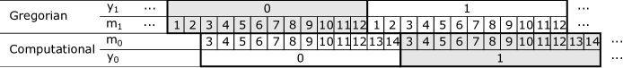
Figure 2: Years $0$ and $1$ in the Gregorian and computational calendars.

If $(y_{0},m_{0},d_{0})\in G_{0}$, then $m_{0}\in[3,15[$ and $d_{0}\in[0,L(y_{1},m_{1})[$ where $(y_{1},m_{1},d_{1})=P_{1}^{-1}(y_{0},m_{0},d_{0})$. (See Table 2.)

Table 2: Months of the computational calendar and their lengths.

$m_{0}$	Name	$L(y_{1},m_{1})$(a)
3	March	31
4	April	30
5	May	31
6	June	30
7	July	31

$m_{0}$	Name	$L(y_{1},m_{1})$(a)
8	August	31
9	September	30
10	October	31
11	November	30
12	December	31

$m_{0}$	Name	$L(y_{1},m_{1})$(b)
13	January	31
14	February	28 or 29 (c)

${(a)}$ $y_{1}=y_{0}$, $m_{1}=m_{0}$. ${(b)}$ $y_{1}=y_{0}+1$, $m_{1}=m_{0}-12$. ${(c)}$ $L(y_{1},m_{1})=29$ if $y_{1}=y_{0}+1$ is a leap year, or $L(y_{1},m_{1})=28$ otherwise.

Remark 4.6.

Table 2 shows that, except for $m_{0}=14$, $m_{0}\mapsto L(y_{1},m_{1})$ is a periodic function and there are $153=31+30+31+30+31$ days in each $5$-month period.

5 A rata die function on the computational calendar

$e_{0}$, the minimum date in $G_{0}$, is undoubtedly the most natural epoch for a rata die function $\rho_{0}$ on $G_{0}$, $\rho_{0}(x_{0})=\#[e_{0},x_{0}[$ for all $x_{0}\in G_{0}$.

For any $x_{0}=(y_{0},m_{0},d_{0})\in G_{0}$, integers $y_{0}$, $m_{0}$, $d_{0}$ and $\rho_{0}(x_{0})$ are non-negative. Hence, implementations of $G_{0}$ can work exclusively on unsigned integer types, which are usually faster than signed ones.

Let $x_{0}=(y_{0},m_{0},d_{0})\in G_{0}$ and split $[e_{0},x_{0}[$ into three disjoint intervals:

$$[e_{0},x_{0}[\ =[(0,3,0),(y_{0},3,0)[\ \cup\ [(y_{0},3,0),(y_{0},m_{0},0)[\ \cup\ [(y_{0},m_{0},0),(y_{0},m_{0},d_{0})[.$$

Hence, $\rho_{0}(x_{0})$ is the sum of the number of elements of these three intervals, which we consider separately.

The year count, defined by $y_{c}(y_{0})=\#[(0,3,0),(y_{0},3,0)[$ is the number of dates prior to year $y_{0}$:

$$y_{c}(y_{0})=365\cdot y_{0}+\#\{y_{0}^{\prime}\in[0,y_{0}[\ ;\ y_{0}^{\prime}\text{ has 366 days }\}$$

Recalling that year $y_{0}^{\prime}$ of the computational calendar has 366 days if, and only if, $y_{0}^{\prime}+1$ is a leap year of the Gregorian calendar gives:

$$y_{c}(y_{0}) =365\cdot y_{0}+\#\{y_{0}^{\prime}\in[0,y_{0}[\ ;\ y_{0}^{\prime}+1\text{ is a leap year }\}$$ (20)

$$=365\cdot y_{0}+\#\{y\in[1,y_{0}+1[\ ;\ y\text{ is a leap year }\}$$

$$=365\cdot y_{0}+\#\{y\in[1,y_{0}]\ ;\ y\%4=0\text{ and }y\%100\neq 0\text{ or }y\%400=0\}$$

$$=365\cdot y_{0}+y_{0}/4-y_{0}/100+y_{0}/400.$$

Remark 5.1.

For all $y_{0}$, $z\in\mathbb{Z}$ with $y_{0}+400\cdot z\geq 0$, we have

$$y_{c}(y_{0}+400\cdot z) =365\cdot(y_{0}+400\cdot z)+(y_{0}+400\cdot z)/4-(y_{0}+400\cdot z)/100+(y_{0}+400\cdot z)/400$$

$$=365\cdot y_{0}+y_{0}/4-y_{0}/100+y_{0}/400+146000\cdot z+100\cdot z-4\cdot z+z$$

$$=y_{c}(y_{0})+146097\cdot z.$$

Hence, by adding $400\cdot z$ years to a date, its rata die increases by $146097\cdot z$. There are $146097$ dates in any $400$-year interval. Such intervals are called leap cycles.

The month count defined by $m_{c}(y_{0},m_{0})=\#[(y_{0},3,0),(y_{0},m_{0},0)[$ is the number of days between the 1st day of year $y_{0}$ and the 1st day of month $m_{0}$ of year $y_{0}$. It can be obtained by adding the lengths of previous months in year $y_{0}$. Since $m_{0}=14$ is the last month of the year, its length is not included in the summation and becomes irrelevant to $m_{c}$. Therefore, the year $y_{0}$ also becomes irrelevant to $m_{c}$, because the last month is the only one whose length depends on the year. In other words, $m_{c}(y_{0},m_{0})=m_{c}(m_{0})$ as per Table 3.

Table 3: Month count.

$m_{0}$	$L(y_{1},m_{1})$	$m_{c}(m_{0})$
3	31	0
4	30	31
5	31	61
6	30	92
7	31	122

$m_{0}$	$L(y_{1},m_{1})$	$m_{c}(m_{0})$
8	31	153
9	30	184
10	31	214
11	30	245
12	31	275

$m_{0}$	$L(y_{1},m_{1})$	$m_{c}(m_{0})$
13	31	306
14	(irrelevant)	337

Some implementations [14, 8, 17] use look-up arrays to recover $m_{c}(m_{0})$, but it can be expressed by an EAF:

$$m_{c}(m_{0})=(153\cdot m_{0}-457)/5,\quad\forall m_{0}\in[3,14].$$ (21)

Variations of this formula have been found by many authors [3, 11, 12, 4, 15, 17, 20, 21], most often through a trial-and-error line fitting to the set of points $\big{\{}(m_{0},m_{c}(m_{0}))\in\mathbb{Z}^{2}\ ;\ m_{0}\in[3,14]\big{\}}$. Remark 4.6 clarifies the matter. However, a simple textbook linear regression on the set $\big{\{}(m_{0},m_{c}(m_{0})+0.5)\in\mathbb{Q}^{2}\ ;\ m_{0}\in[3,14]\big{\}}$ finds $m_{c}(m_{0})=(26256\cdot m_{0}-78317)/858$. Using this EAF in Theorem 3.4 produces the same faster alternative seen in Example 3.5.

The day count defined by $d_{c}(y_{0},m_{0},d_{0})=\#[(y_{0},m_{0},0),(y_{0},m_{0},d_{0})[$ is the number of dates since the 1st of month $m_{0}$ of year $y_{0}$. Trivially, $d_{c}(y_{0},m_{0},d_{0})=d_{0}$.

Putting together the above results yields the next proposition.

Proposition 5.2.

Let $(y_{0},m_{0},d_{0})\in G_{0}$. Set:

$$y_{c} =365\cdot y_{0}+y_{0}/4-y_{0}/100+y_{0}/400, m_{c} =(153\cdot m_{0}-457)/5, d_{c} =d_{0}.$$

Then, $\rho_{0}(y_{0},m_{0},d_{0})=y_{c}+m_{c}+d_{c}$.

The calculations of Proposition 5.2 can be performed more efficiently by first computing the century.

Corollary 5.3.

Let $(y_{0},m_{0},d_{0})\in G_{0}$. Set:

$$q_{1} =y_{0}/100, y_{c} =1461\cdot y_{0}/4-q_{1}+q_{1}/4, m_{c} =(979\cdot m_{0}-2919)/2^{5}, d_{c} =d_{0}.$$

Then, $\rho_{0}(y_{0},m_{0},d_{0})=y_{c}+m_{c}+d_{c}$.

Proof.

It suffices to show that the following alternatives for the expressions seen in Proposition 5.2 hold.

1. $1461\cdot y_{0}/4=365\cdot y_{0}+y_{0}/4$: This follows from $1461\cdot y_{0}=4\cdot(365\cdot y_{0}+y_{0}/4)+y_{0}\%4$ and $0\leq y_{0}\%4<4$.

2. $(153\cdot m_{0}-457)/5=(979\cdot m_{0}-2919)/2^{5}$: This follows from $m_{0}\in[3,14]$ and Equation 8.

3. $y_{0}/400=q_{1}/4$: This follows from $y_{0}/100/4=y_{0}/400$.

∎

5.1 Inverting the rata die function on the computational calendar

The computational calendar $G_{0}$ is unbounded from above and, thus, for any $r_{0}\in\mathbb{Z^{+}}$ a unique $x_{0}\in G_{0}$ exists such that $\rho_{0}(x_{0})=r_{0}$. The objective of this section is to find $x_{0}$ given that $r_{0}$.

For $x_{0}=(y_{0},m_{0},d_{0})\in G_{0}$, the quotient $q=y_{0}/100$ is its century. Since $100\cdot q\leq y_{0}<100\cdot(q+1)$, we have $(100\cdot q,3,0)\leq x_{0}<(100\cdot(q+1),3,0)$. The quantity $\#[(100\cdot q,3,0),x_{0}[$ is the day of the century of $x_{0}$. The next proposition retrieves the century and the day of the century from a rata die.

Proposition 5.4.

Let $x_{0}\in G_{0}$ and $r_{0}$ be its rata die. Set:

$$n_{1} =4\cdot r_{0}+3, q_{1} =n_{1}/146097, r_{1} =n_{1}\%146097/4.$$

Then, $q_{1}$ is the century of $x_{0}$ and $r_{1}$ is its day of the century.

Proof.

Write $x_{0}=(y_{0},m_{0},d_{0})$ and set $q=y_{0}/100$ and $r=\#[(100\cdot q,3,0),x_{0}[$. We must prove that $q_{1}=q$ and $r_{1}=r$.

For $p\in\mathbb{Z^{+}}$, let $g(p)=\#[e_{0},(100\cdot p,3,0)[$. The definition of $y_{c}$ gives $g(p)=y_{c}(100\cdot p)$ and Equation 20 yields

$$g(p) =365\cdot 100\cdot p+100\cdot p/4-100\cdot p/100+100\cdot p/400=36524\cdot p+p/4$$

$$=146097\cdot p/4.$$

(The last equality is obtained as Item (i) in the proof of Corollary 5.3, using $36524$ instead of $365$.)

Since $r_{0}=\#[e_{0},x_{0}[\ =\#[e_{0},(100\cdot q,3,0)[\ +\ \#[(100\cdot q,3,0),x_{0}[$, we have $r_{0}=g(q)+r\geq g(q)$. Now, $x_{0}<(100\cdot(q+1),3,0)$ and $r_{0}=\#[e_{0},x_{0}[\ <\#[e_{0},(100\cdot(q+1),3,0)[\ =g(q+1)$. Hence, $r_{0}<g(q+1)$, in other words, $r_{0}\in[g(q),g(q+1)[$. As seen in Example 2.6 (where $\hat{f}=g$):

$$(4\cdot r_{0}+3)/146097=q\quad\text{and}\quad(4\cdot r_{0}+3)\%146097/4=r_{0}-g(q).$$

These equalities mean that $q_{1}=q$ and $r_{1}=r$. ∎

For $x_{0}=(y_{0},m_{0},d_{0})\in G_{0}$, the remainder $y_{0}\%100$ is its year of the century. We have $(y_{0},3,0)\leq x_{0}<(y_{0}+1,3,0)$ and the quantity $\#[(y_{0},3,0),x_{0}[$ is called the day of the year of $x_{0}$. The next proposition starts where Proposition 5.4 left off, i.e., at the day of the century, to obtain the year of the century and the day of the year.

Proposition 5.5.

Let $x_{0}\in G_{0}$ and $r_{1}$ be its day of the century. Set:

$$n_{2} =4\cdot r_{1}+3, q_{2} =n_{2}/1461, r_{2} =n_{2}\%1461/4.$$

Then, $q_{2}$ is the year of the century of $x_{0}$ and $r_{2}$ is its day of the year.

Proof.

Write $x_{0}=(y_{0},m_{0},d_{0})$ and set $q_{1}=y_{0}/100$, $q=y_{0}\%100$ and $r=\#[(y_{0},3,0),x_{0}[$. We must prove that $q_{2}=q$ and that $r_{2}=r$.

For $p\in[0,100[$, it is easy to show that $(100\cdot q_{1}+p)/100=100\cdot q_{1}/100$ and $(100\cdot q_{1}+p)/400=q_{1}/4$. Let $g(p)=\#[(100\cdot q_{1},3,0),(100\cdot q_{1}+p,3,0)[$. The definition of $y_{c}$ gives $g(p)=y_{c}(100\cdot q_{1}+p)-y_{c}(100\cdot q_{1})$ and Equation 20 yields:

$$g(p) =365\cdot(100\cdot q_{1}+p)+(100\cdot q_{1}+p)/4-(100\cdot q_{1}+p)/100+(100\cdot q_{1}+p)/400-y_{c}(100\cdot q_{1})$$

$$=365\cdot p+p/4=1461\cdot p/4.$$

(The last equality is the same as Item (i) in the proof of Corollary 5.3.)

Since $y_{0}=100\cdot q_{1}+q$ and $r_{1}=\#[(100\cdot q_{1},3,0),x_{0}[$, we have

$$r_{1} =\#[(100\cdot q_{1},3,0),(y_{0},3,0)[\ +\ \#[(y_{0},3,0),x_{0}[$$

$$=\#[(100\cdot q_{1},3,0),(100\cdot q_{1}+q,3,0)[\ +\ \#[(y_{0},3,0),x_{0}[\ =g(q)+r\geq g(q).$$

Since $x_{0}<(y_{0}+1,3,0)=(100\cdot q_{1}+q+1,3,0)$, we have $r_{1}<\#[(100\cdot q_{1},3,0),(100\cdot q_{1}+q+1,3,0)[\ =g(q+1)$ and it follows that $r_{1}\in[g(q),g(q+1)[$. As seen in Example 2.7 (where $\hat{f}=g$):

$$(4\cdot r_{1}+3)/1461=q\quad\text{and}\quad(4\cdot r_{1}+3)\%1461/4=r_{1}-g(q).$$

These equalities mean that $q_{2}=q$ and that $r_{2}=r$. ∎

Like Proposition 5.5, the following result provides calculations for year of century and day of year, but in a computationally more efficient way.

Corollary 5.6.

Let $x_{0}\in G_{0}$ and $r_{1}$ be its day of the century. Set:

$$n_{2} =4\cdot r_{1}+3, u_{2} =2\ \!939\ \!745\cdot n_{2}, q_{2} =u_{2}/2^{32}, r_{2} =u_{2}\%2^{32}/2\ \!939\ \!745/4.$$

Then, $q_{2}$ is the year of the century of $x_{0}$ and $r_{2}$ is its day of the year.

Proof.

Example 3.12 shows that the $q_{2}$ and $r_{2}$ set above match those of Proposition 5.5, provided that $n_{2}\in[0,28\ \!825\ \!529[$, which we shall prove now. Proposition 5.4 provides that $r_{1}=n_{1}\%146097/4$ for some $n_{1}\in\mathbb{Z}$. From $0\leq n_{1}\%146097<146097$, it easily follows that $3\leq 4\cdot r_{1}+3<146100$, in other words, $n_{2}\in[3,146100[$. ∎

The following proposition extracts the month and day from the day of the year.

Proposition 5.7.

Let $x_{0}\in G_{0}$ and $r_{2}$ be its day of the year. Set:

$$n_{3} =5\cdot r_{2}+461, q_{3} =n_{3}/153, r_{3} =n_{3}\%153/5.$$

Then, $q_{3}$ is the month of $x_{0}$ and $r_{3}$ is its day.

Proof.

Let $x_{0}=(y_{0},m_{0},d_{0})$. We must prove that $q_{3}=m_{0}$ and that $r_{3}=d_{0}$.

For $p\in[3,15]$, let $g(p)=(153\cdot p-457)/5$. Equation 21 provides that if $p\in[3,14]$, then $g(p)=m_{c}(p)=\#[(y_{0},3,0),(y_{0},p,0)[$. By definition, $r_{2}=\#[(y_{0},3,0),x_{0}[$ can be written as:

$$r_{2} =\#[(y_{0},3,0),(y_{0},m_{0},0)[\ +\ \#[(y_{0},m_{0},0),(y_{0},m_{0},d_{0})[\ =g(m_{0})+d_{0}\geq g(m_{0}).$$

We shall now prove that $r_{2}<g(m_{0}+1)$. If $m_{0}<14$, then $x_{0}<(y,m_{0}+1,0)$ and we obtain $r_{2}=\#[(y_{0},3,0),x_{0}[\ <\#[(y_{0},3,0),(y_{0},m_{0}+1,0)[\ =m_{c}(m_{0}+1)=g(m_{0}+1)$. Now, if $m_{0}=14$, then $x_{0}\leq(y_{0},14,L(y_{0},2))$ and it follows that $r_{2}\leq\#[(y_{0},3,0),(y_{0},14,L(y_{0},2))]\leq 366<367=g(15)=g(m_{0}+1)$. Hence, $r_{2}<g(m_{0}+1)$, in other words, $r_{2}\in[g(m_{0}),g(m_{0}+1)[$. As seen in Example 2.8 (where $\hat{f}=g$):

$$(5\cdot r_{2}+461)/153=m_{0}\quad\text{and}\quad(5\cdot r_{2}+461)\%153/5=r_{2}-g(m_{0}).$$

These equalities mean that $q_{3}=m_{0}$ and that $r_{3}=d_{0}$. ∎

Remark 5.8.

In the proof of Proposition 5.7, we have shown that if $r_{2}$ is the day of the year of $(y_{0},m_{0},d_{0})\in G_{0}$ and $m_{0}<14$, then $r_{2}\in[m_{c}(m_{0}),m_{c}(m_{0}+1)[$. It follows that $m_{0}\geq 13$ is equivalent to $r_{2}\geq m_{c}(13)=306$.

Again, the following corollary improves the computational efficiency of the calculations of Proposition 5.7.

Corollary 5.9.

Let $x_{0}\in G_{0}$ and $r_{2}$ be its day of the year. Set:

$$n_{3} =2141\cdot r_{2}+197913, q_{3} =n_{3}/2^{16}, r_{3} =n_{3}\%2^{16}/2141.$$

Then, $q_{3}$ is the month of $x_{0}$ and $r_{3}$ is its day.

Proof.

Example 3.13 shows that the $q_{3}$ and $r_{3}$ set above match those of Proposition 5.7, provided that $r_{2}\in[0,734[$, which we shall prove now. Proposition 5.5 provides that $r_{2}=n_{2}\%1461/4$ for some $n_{2}\in\mathbb{Z}$. From $0\leq n_{2}\%1461<1461$, it easily follows that $0\leq r_{2}\leq 365$. ∎

6 Rata die functions on the Gregorian calendar

Section 5 covered evaluation of a rata die function and its inverse on the computational calendar $G_{0}$. This section adapts them to the Gregorian calendar.

$G_{0}$ allows implementations to work exclusively on unsigned integer types, which might be faster than signed ones. To avoid compromising this advantage, we only consider subsets of $G$ that have a minimum. These calendars, their respective rata die functions and epochs are summarised in Table 4. For ease of reference, the first row is a reminder for $G_{0}$.

Table 4: Gregorian-related calendars.

Calendar	Rata die	Epoch
$G_{0}=P_{1}(G_{1})$, where $G_{1}$ is defined below.	$\rho_{0}:G_{0}\rightarrow\mathbb{Z}$	$e_{0}=(0,3,0)=P_{1}(e_{1})$
$G_{1}=\{x_{1}\in G\ ;\ x_{1}\geq e_{1}\}$	$\rho_{1}:G_{1}\rightarrow\mathbb{Z}$	$e_{1}=(0,3,1)$
$G_{2}=\{x_{2}\in G\ ;\ x_{2}\geq e_{2}\}$	$\rho_{2}:G_{2}\rightarrow\mathbb{Z}$	$e_{2}=(z_{2},3,1)$, where $z_{2}$ is a multiple of $400$.
$G_{2}$ (as above)	$\rho_{3}:G_{2}\rightarrow\mathbb{Z}$	$e_{3}\in G_{2}$.

The rows of Table 4 show increasing degrees of freedom of how epochs and minima can be set. For $G_{0}$ and $\rho_{0}$ there are no choices: epoch and the minimum date are set to $e_{0}=(0,3,0)$. A match between the epoch and the minimum implies that $\rho_{0}$ is non-negative. Since $e_{0}$’s year is zero, dates in $G_{0}$ have non-negative years. The same holds for $G_{1}$, $\rho_{1}$ and $e_{1}=(0,3,1)$. For $G_{2}$ and $\rho_{2}$, epoch and minimum also match and are set to $e_{2}=(z_{2},3,1)$, but $z_{2}$ can be any multiple of $400$. Therefore, $\rho_{2}$ is also non-negative, although negative years are possible when $z_{2}<0$. Finally, $\rho_{3}$ provides a more flexible setting where any epoch and minimum can be chosen.

As we shall see, $\rho_{1}=\rho_{0}\circ P_{1}$. In general, maps from one calendar to another provide a way to express rata die functions. Conversely, rata die functions provide a way to map one calendar into another [12, 20, 21].

Proposition 6.1.

Let $C$ and $C^{\prime}$ be calendars and let $\rho$ and $\rho^{\prime}$ be their respective rata die functions with epochs $e\in C$ and $e^{\prime}\in C^{\prime}$. If $P:C\rightarrow C^{\prime}$ is a strictly increasing bijection and $P(e)=e^{\prime}$, then $\rho=\rho^{\prime}\circ P$ and $\rho^{-1}=P^{-1}\circ\rho^{\prime-1}$ on $Im(\rho^{\prime})=Im(\rho)$. Conversely, if $Im(\rho)=Im(\rho^{\prime})$, then $\rho^{\prime-1}\circ\rho$ is a strictly increasing bijection from $C$ to $C^{\prime}$.

Proof.

Let $x\in C$ and assume that $x\geq e$. Since $P$ is a strictly increasing bijection, we have $\rho(x)=\#[e,x[\ =\#P([e,x[)=\#[P(e),P(x)[)=\#[e^{\prime},P(x)[\ =\rho^{\prime}(P(x))$. The case $x<e$ is treated analogously and we conclude that $\rho=\rho^{\prime}\circ P$. From this and well-known results on functions and their inverses, we obtain $\rho^{-1}=P^{-1}\circ\rho^{\prime-1}$ on $Im(\rho^{\prime})=Im(\rho)$.

By definition, $\rho(x)\in Im(\rho)=Im(\rho^{\prime})$ and $\rho^{\prime-1}(\rho(x))\in C^{\prime}$, in other words, $\rho^{\prime-1}\circ\rho$ is a map from $C$ to $C^{\prime}$. Since $\rho:C\rightarrow\mathbb{Z}$ and $\rho^{\prime-1}:Im(\rho^{\prime})\rightarrow C^{\prime}$ are strictly increasing surjective functions, hence bijections, their composition is again a strictly increasing bijection. ∎

6.1 The non-negative rata die with epoch 1 March 0000

This section concerns the rata die function $\rho_{1}$ on $G_{1}=\{x_{1}\in G\ ;\ x_{1}\geq e_{1}\}$ with epoch $e_{1}=(0,3,1)$.

From Remark 4.5 and Proposition 6.1 applied to $C=G_{1}$, $C^{\prime}=G_{0}$, $\rho=\rho_{1}$, $\rho^{\prime}=\rho_{0}$, $e=e_{1}$, $e^{\prime}=e_{0}$ and $P=P_{1}$ we obtain:

$$(y_{1},m_{1},d_{1})\in G_{1}\quad\Longrightarrow\quad P_{1}(y_{1},m_{1},\rho_{1})\in G_{0}\quad\text{and}\quad\rho_{1}(y_{1},m_{1},d_{1})=\rho_{0}\left(P_{1}(y_{1},m_{1},d_{1})\right)$$ (22)

and, conversely,

$$(y_{0},m_{0},d_{0})\in G_{0}\quad\Longrightarrow\quad P_{1}^{-1}(y_{0},m_{0},\rho_{0})\in G_{1}\quad\text{and}\quad\rho_{0}(y_{0},m_{0},d_{0})=\rho_{1}\left(P_{1}^{-1}(y_{0},m_{0},d_{0})\right).$$ (23)

6.2 Rata die with a chosen epoch

Let $z_{2}\in\mathbb{Z}$ be a multiple of $400$ and $e_{2}=(z_{2},3,1)$. This section concerns two rata die functions: $\rho_{2}$ on $G_{2}=\{x_{2}\in G\ ;\ x_{2}\geq e_{2}\}$ with epoch $e_{2}$, and $\rho_{3}$ also on $G_{2}$ but with epoch $e_{3}\in G_{2}$ arbitrarily chosen.

Let $P_{2}:\mathbb{Z}^{3}\rightarrow\mathbb{Z}^{3}$ be the map $P_{2}(y_{2},m_{2},d_{2})=(y_{2}-z_{2},m_{2},d_{2})$, which is a strictly increasing bijection with $P_{2}^{-1}(y_{1},m_{1},d_{1})=(y_{1}+z_{2},m_{1},d_{1})$ and $P_{2}(e_{2})=(0,3,1)=e_{1}$.

Let $(y_{2},m_{2},d_{2})\in G_{2}$ and set $(y_{1},m_{1},d_{1})=P_{2}(y_{2},m_{2},d_{2})$. We have $m_{1}=m_{2}\in[1,12]$, $d_{1}=d_{2}\in[1,L(y_{2},m_{2})]$ and, since $z_{2}\%400=0$, $y_{2}-z_{2}$ is a leap year if, and only if, $y_{2}$ is a leap year. Hence, $L(y_{2},m_{2})=L(y_{2}-z_{2},m_{2})=L(y_{1},m_{1})$ and it follows that $d_{1}\in[1,L(y_{1},m_{1})]$. Therefore, $(y_{1},m_{1},d_{1})\in G$. From $(y_{2},m_{2},d_{2})\geq e_{2}$, we obtain $(y_{1},m_{1},d_{1})\geq e_{1}$ and conclude that $(y_{1},m_{1},d_{1})\in G_{1}$. Similarly, we can show that $P_{2}^{-1}(y_{1},m_{1},d_{1})\in G_{2}$ for all $(y_{1},m_{1},d_{1})\in G_{1}$ and thus, $P_{2}$ is a bijection from $G_{2}$ to $G_{1}$.

Applying Proposition 6.1 to $C=G_{2}$, $C^{\prime}=G_{1}$, $\rho=\rho_{2}$, $\rho^{\prime}=\rho_{1}$, $e=e_{2}$, $e^{\prime}=e_{1}$ and $P=P_{2}$ gives:

$$(y_{2},m_{2},d_{2})\in G_{2}\quad\Longrightarrow\quad(y_{2}-z_{2},m_{2},d_{2})\in G_{1}\quad\text{and}\quad\rho_{2}(y_{2},m_{2},d_{2})=\rho_{1}(y_{2}-z_{2},m_{2},d_{2})$$ (24)

and, reciprocally,

$$(y_{1},m_{1},d_{1})\in G_{1}\quad\Longrightarrow\quad(y_{1}+z_{2},m_{1},d_{1})\in G_{2}\quad\text{and}\quad\rho_{1}(y_{1},m_{1},d_{1})=\rho_{2}(y_{1}+z_{2},m_{1},d_{1}).$$ (25)

Fix $e_{3}\in G_{2}$ and let $\rho_{3}:G_{2}\rightarrow\mathbb{Z}$ be the rata die function with epoch $e_{3}$. Let $x_{2}\in G_{2}$. On the one hand, if $x_{2}\geq e_{3}$, then $\#[e_{2},x_{2}[\ =\#[e_{2},e_{3}[\ +\ \#[e_{3},x_{2}[$, in other words, $\rho_{2}(x_{2})=\rho_{2}(e_{3})+\rho_{3}(x_{2})$. On the other hand, if $x_{2}<e_{3}$, then $\#[e_{2},e_{3}[\ =\#[e_{2},x_{2}[\ +\ \#[x_{2},e_{3}[$, in other words, $\rho_{2}(e_{3})=\rho_{2}(x_{2})-\rho_{3}(x_{2})$. Therefore,

$$x_{2}\in G_{2}\quad\Longrightarrow\quad\rho_{3}(x_{2})=\rho_{2}(x_{2})-\rho_{2}(e_{3}).$$ (26)

The next two propositions prove the correctness of our Gregorian calendar algorithms. Proposition 6.2 considers the calculation of the rata die function for any chosen epoch and Proposition 6.3 considers its inverse.

Proposition 6.2.

Let $\rho_{2}$, $\rho_{3}$ be rata die functions on $G_{2}$ with epochs $e_{2}=(z_{2},3,1)$ and $e_{3}$, respectively, where $z_{2}\in\mathbb{Z}$ is a multiple of $400$. Given $(y_{2},m_{2},d_{2})\in G_{2}$, set:

$$\begin{aligned} y_{1}&=y_{2}-z_{2},\\ m_{1}&=m_{2},\\ d_{1}&=d_{2},\\ \end{aligned}\quad\vrule\quad\begin{aligned} y_{0}&=y_{1}-{\bf 1}_{\{m_{1}\leq 2\}},\\ m_{0}&=m_{1}+12\cdot{\bf 1}_{\{m_{1}\leq 2\}},\\ d_{0}&=d_{1}-1,\end{aligned}\quad\vrule\quad\begin{aligned} q_{1}&=y_{0}/100,\\ y_{c}&=1461\cdot y_{0}/4-q_{1}+q_{1}/4,\\ m_{c}&=(979\cdot m_{0}-2919)/2^{5},\\ d_{c}&=d_{0}.\end{aligned}$$

Then, $\rho_{3}(y_{2},m_{2},d_{2})=y_{c}+m_{c}+d_{c}-\rho_{2}(e_{3})$.

Proof.

The first column and Equation 24 give $(y_{1},m_{1},d_{1})\in G_{1}$ and $\rho_{2}(y_{2},m_{2},d_{2})=\rho_{1}(y_{1},m_{1},d_{1})$. The second column gives $(y_{0},m_{0},d_{0})=P_{1}(y_{1},m_{1},d_{1})$ and Equation 22 yields $(y_{0},m_{0},d_{0})\in G_{0}$ and $\rho_{1}(y_{1},m_{1},d_{1})=\rho_{0}(y_{0},m_{0},d_{0})$. Hence, $\rho_{2}(y_{2},m_{2},d_{2})=\rho_{0}(y_{0},m_{0},d_{0})$, and from Corollary 5.3 we obtain $\rho_{2}(y_{2},m_{2},d_{2})=y_{c}+m_{c}+d_{c}$. The result follows from Equation 26. ∎

Proposition 6.3.

Let $\rho_{2}$, $\rho_{3}$ be rata die functions on $G_{2}$ with epochs $e_{2}=(z_{2},3,1)$ and $e_{3}\geq e_{2}$, respectively, where $z_{2}\in\mathbb{Z}$ is a multiple of $400$. Given $r\in\mathbb{Z}$ with $r\geq-\rho_{2}(e_{3})$, set $r_{0}=r+\rho_{2}(e_{3})$ and:

$$\begin{aligned} n_{1}&=4\cdot r_{0}+3,\\ \\ q_{1}&=n_{1}/146097,\\ r_{1}&=n_{1}\%146097/4,\\ \end{aligned}\quad\vrule\quad\begin{aligned} n_{2}&=4\cdot r_{1}+3,\\ u_{2}&=2\ \!939\ \!745\cdot n_{2},\\ q_{2}&=u_{2}/2^{32},\\ r_{2}&=u_{2}\%2^{32}/2\ \!939\ \!745/4,\\ \end{aligned}\quad\vrule\quad\begin{aligned} n_{3}&=2141\cdot r_{2}+197913,\\ \\ q_{3}&=n_{3}/2^{16},\\ r_{3}&=n_{3}\%2^{16}/2141.\\ \end{aligned}$$

and:

$$\begin{aligned} y_{0}&=100\cdot q_{1}+q_{2},\\ m_{0}&=q_{3},\\ d_{0}&=r_{3},\\ \end{aligned}\quad\vrule\quad\begin{aligned} y_{1}&=y_{0}+{\bf 1}_{\{r_{2}\geq 306\}},\\ m_{1}&=m_{0}-12\cdot{\bf 1}_{\{r_{2}\geq 306\}},\\ d_{1}&=d_{0}+1.\\ \end{aligned}\quad\vrule\quad\begin{aligned} y_{2}&=y_{1}+z_{2},\\ m_{2}&=m_{1},\\ d_{2}&=d_{1}.\end{aligned}$$ (27)

Then, $\rho_{3}(y_{2},m_{2},d_{2})=r$.

Proof.

Since $r\geq-\rho_{2}(e_{3})$, we have $r_{0}=r+\rho_{2}(e_{3})\geq 0$ and thus $x_{0}\in G_{0}$ exists such that $\rho(x_{0})=r_{0}$.

Proposition 5.4 provides that $q_{1}$ is the century of $x_{0}$ and that $r_{1}$ is its day of the century. Corollary 5.6 then yields that $q_{2}$ is the year of the century of $x_{0}$ and $r_{2}$ is its day of the year, while Corollary 5.9 states that $q_{3}$ is the month of $x_{0}$ and $r_{3}$ is its day.

Hence, the first column of Equation 27 reads $x_{0}=(y_{0},m_{0},d_{0})$. From Remark 5.8 we can substitute ${\bf 1}_{\{r_{2}\geq 306\}}$ with ${\bf 1}_{\{m_{0}\geq 13\}}$ and then, by Equation 19 the second column of Equation 27 becomes $(y_{1},m_{1},d_{1})=P_{1}^{-1}(x_{0})$ and Equation 23 gives $(y_{1},m_{1},d_{1})\in G_{1}$ and $\rho_{1}(y_{1},m_{1},d_{1})=\rho_{0}(x_{0})$. Finally, Equation 25 and the third column of Equation 27 yield $(y_{2},m_{2},d_{2})\in G_{2}$ and $\rho_{2}(y_{2},m_{2},d_{2})=\rho_{1}(y_{1},m_{1},d_{1})=\rho_{0}(x_{0})=r_{0}=r+\rho_{2}(e_{3})$.

We have shown that $r=\rho_{2}(y_{2},m_{2},d_{2})-\rho_{2}(e_{3})$. Therefore, Equation 26 gives $\rho_{3}(y_{2},m_{2},d_{2})=r$. ∎

7 Performance analysis

We benchmarked our algorithms from Propositions 6.2 and 6.3 against counterparts in five of the most widely used C, C++, C# and Java libraries, as listed below:

glibc	The GNU C Library [7, 8]. (The Linux Kernel contains a similar implementation [14].)
Boost	The Boost C++ libraries [4].
libc++	LLVM’s implementation of the C++ Standard Library [15].
.NET	Microsoft .NET framework [17].
OpenJDK	Oracle’s open source implementation of the Java Platform SE [19]. (Android uses the same code [2].)

We used source files as publicly available on 2 May 2020. Non-C++ implementations have been ported to this language and have all been slightly modified to achieve consistent (a) function signatures; (b) storage types (for years, months, days and rata dies); and (c) epoch (Unix epoch, i.e., 1 January 1970). Some originals deal with date and time but our variants work on dates only. (Given the uniform durations of days, hours, minutes and seconds, it would be trivial to incorporate the time component to any dates-only algorithm. Moreover, Example 3.14 suggests improvements that are not used by major implementations.)

We did not include Microsoft’s C++ Standard Library because in May 2020 it did not yet implement these functionalities. For the same reason, libstdc++, the GNU implementation of the C++ Standard Library, is also absent. Furthermore, a forthcoming release of libstdc++ is expected to implement our algorithms.

We also considered our own implementations of algorithms described in the academic literature, namely, Baum [3], Fliegel and Flandern [6], Hatcher [11, 12, 21] and Reingold and Dershovitz [20].

Timings were obtained with the help of the Google Benchmark library [9], to which we delegated the task of producing statistically relevant results. The code was run on an Intel i7-10510U CPU at $4.9$ GHz. Source code, available at [18], was compiled by GCC 10.2.0 at optimisation level -O3. Results vary across platforms but maintain qualitative consistency between them.

The table in Figure 3 shows the time taken by each algorithm to evaluate $\rho_{3}$ at $16\ \!384$ pseudo-random dates, uniformly distributed in $[(1570,1,1),(2370,1,1)[$ (i.e., Unix epoch $\pm 400$ years). They encompass the time spent scanning the array of dates (also shown). Subtracting the scanning time from that of each algorithm gives a fairer account of the time spent by the algorithm itself. The chart plots these adjusted timings relative to ours (Proposition 6.2).

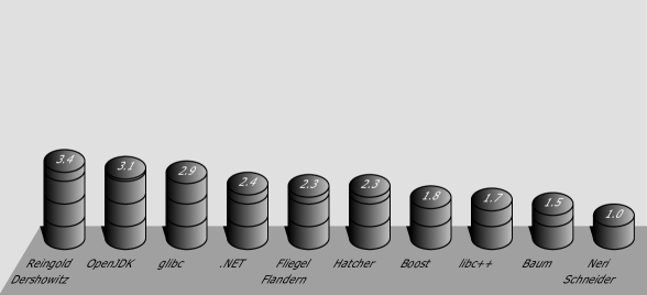
Algorithm	Time (ns)
scanning only	3 ​430.3
Reingold Dershowitz	76 ​523.4
OpenJDK	69 ​906.5
glibc	64 ​891.2
.NET	55 ​179.5
Hatcher	52 ​494.6
Fliegel Flandern	53 ​893.4
Boost	41 ​281.2
libc++	39 ​309.4
Baum	35 ​263.8
Neri Schneider	24 ​963.3

Figure 3: Relative and absolute timings of rata die evaluations.

Similarly, the table in Figure 4 shows the time taken by each algorithm to evaluate $\rho_{3}^{-1}$ at $16384$ pseudo-random integer numbers uniformly distributed in $[-146097,146097[$ (again, Unix epoch $\pm 400$ years as per Remark 5.1). The chart displays adjusted times relative to ours (Proposition 6.3).

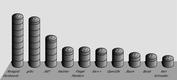
Algorithm	Time (ns)
scanning only	3 ​429.1
Reingold Dershowitz	372 ​984.0
glibc	350 ​648.0
.NET	206 ​279.0
Hatcher	119 ​239.0
Fliegel Flandern	117 ​635.0
libc++	107 ​537.0
OpenJDK	106 ​850.0
Baum	76 ​516.2
Boost	65 ​564.4
Neri Schneider	50 ​770.3

Figure 4: Relative and absolute timings of rata die inverse evaluations.

Disclaimer

Opinions and estimates constitute our judgement as of the date of this Material, are for informational purposes only and are subject to change without notice. This Material is not the product of J.P. Morgan’s Research Department and therefore, has not been prepared in accordance with legal requirements to promote the independence of research, including but not limited to, the prohibition on the dealing ahead of the dissemination of investment research. This Material is not intended as research, a recommendation, advice, offer or solicitation for the purchase or sale of any financial product or service, or to be used in any way for evaluating the merits of participating in any transaction. It is not a research report and is not intended as such. Past performance is not indicative of future results. Please consult your own advisors regarding legal, tax, accounting or any other aspects including suitability implications for your particular circumstances. J.P. Morgan disclaims any responsibility or liability whatsoever for the quality, accuracy or completeness of the information herein, and for any reliance on, or use of this material in any way. Important disclosures at: www.jpmorgan.com/disclosures

References

[1]
R. Alverson.
Integer division using reciprocals.
In [1991] Proceedings 10th IEEE Symposium on Computer
Arithmetic, pages 186–190, 1991.
doi.org/10.1109/ARITH.1991.145558.
[2]
Android.
ojluni/src/main/java/java/time/LocalDate.java.
tinyurl.com/ycsltdnq, April
2017.
[4]
Boost C++ Libraries.
include/boost/date_time/gregorian_calendar.ipp.
tinyurl.com/y4buxmmf, March
2020.
[5]
D. Cavagnino and A. E. Werbrouck.
Efficient algorithms for integer division by constants using
multiplication.
The Computer Journal, 51(4):470–480, 11 2007.
doi.org/10.1093/comjnl/bxm082.
[6]
Henry F. Fliegel and Thomas C. van Flandern.
Letters to the editor: A machine algorithm for processing calendar
dates.
Communications of the ACM, 11(10):657–658, 10 1968.
doi.org/10.1145/364096.364097.
[10]
Torbjörn Granlund and Peter L. Montgomery.
Division by invariant integers using multiplication.
In Proceedings of the ACM SIGPLAN 1994 Conference on Programming
Language Design and Implementation, PLDI ’94, pages 61–72, New York, NY,
USA, 1994. Association for Computing Machinery.
doi.org/10.1145/178243.178249.
[11]
D. A. Hatcher.
Simple formulae for julian day numbers and calendar dates.
Quarterly Journal of the Royal Astronomical Society,
25(1):55–53, 03 1984.
tinyurl.com/y2orpwfr.
[12]
D. A. Hatcher.
Generalized equations for julian day numbers and calendar dates.
Quarterly Journal of the Royal Astronomical Society,
26(2):151–155, 06 1985.
tinyurl.com/y6ec7t3h.
[13]
Daniel Lemire, Owen Kaser, and Nathan Kurz.
Faster remainder by direct computation: Applications to compilers and
software libraries.
Software: Practice and Experience, 49(6):953–970, 2019.
doi.org/10.1002/spe.2689.
[16]
D. J. Magenheimer, L. Peters, K. W. Pettis, and D. Zuras.
Integer multiplication and division on the hp precision architecture.
IEEE Transactions on Computers, 37(8):980–990, 1988.
doi.org/10.1109/12.2248.
[17]
Microsoft .NET.
src/libraries/System.Private.CoreLib/src/System/DateTime.cs.
tinyurl.com/y4kej3mm, April
2020.
[19]