Identifying symmetries and predicting cluster synchronization in complex networks

Abstract

Symmetries in a network connectivity regulate how the graph’s functioning organizes into clustered states. Classical methods for tracing the symmetry group of a network require very high computational costs, and therefore they are of hard, or even impossible, execution for large sized graphs. We here unveil that there is a direct connection between the elements of the eigen-vector centrality and the clusters of a network. This gives a fresh framework for cluster analysis in undirected and connected graphs, whose computational cost is linear in $N$. We show that the cluster identification is in perfect agreement with symmetry based analyses, and it allows predicting the sequence of synchronized clusters which form before the eventual occurrence of global synchronization.

Synchronization in dynamical networks is one of the most common collective properties emerging in real and man made systems, from power grids to neuronal firing  Strogatz (2004); Boccaletti et al. (2006); Dorfler and Bullo (2012); Motter et al. (2013); Ashwin et al. (2016); Boccaletti et al. (2018). In particular, complete, or global, synchronization (GS) is the state where all the identical units of a system evolve in unison. Yet, in some instances GS is either undesirable (it actually corresponds to pathological states of the brain) or is not attained. Rather, the network organizes into structure dependent synchronization states, such as cluster (CS) or remote synchronization Dahms et al. (2012); Skardal et al. (2011); Nicosia et al. (2013); Sorrentino and Ott (2007); Williams et al. (2013); Pecora et al. (2014); Sorrentino et al. (2016); Lodi et al. (2020); Bergner et al. (2012); Sorrentino and Pecora (2016); Gambuzza and Frasca (2019); Siddique et al. (2018); Sorrentino et al. (2016); Wang et al. (2019); Karakaya et al. (2019); Zhang et al. (2017). In CS, a set of units form a synchronized cluster Nicosia et al. (2013); Cho et al. (2017); Pecora et al. (2014); Della Rossa et al. (2020); Sorrentino et al. (2020) with the rest of the network evolving asynchronously. Swarms of animals, or synchronous states (within sub units) in power grids, or brain dynamics are relevant examples of such CS Sorrentino et al. (2016). In graph theoretic perspective, these clusters are the orbits of the graph and are the ingredients of the associated symmetry groups. The stability of such synchronous clusters depends on the analysis of the symmetry group elements Pecora et al. (2014).

Identifying the symmetries of a network is, therefore, of paramount importance, as it allows predicting the details of how the system’s functioning organizes into synchronized clusters. However, tracing the entire symmetry group of a network is not an easy task. It involves determining all symmetry group elements by a brute-force checking of permutations, a procedure which requires a number of operations which is non polynomial with the number $N$ of nodes, and therefore of hard (or even impossible) execution for large sized graphs.

Against this backdrop, in this Letter we introduce a general method through which one can identify the orbits or clusters of a network without the need of exploring its symmetry group. In particular, we analytically prove that there is a direct connection between the elements of the eigen-vector centrality (EVC) and the clusters of the network. The EVC is the eigen-vector of the network’s adjacency matrix corresponding to the largest eigen-value Pradhan et al. (2020); Newman (2010), and therefore the cost of its evaluation scales linearly with $N$. We then propose a novel framework to unveil clusters in a generic undirected, connected, and positive semidefinite graph, and show that the clusters identified are in perfect agreement with the ones determined from the symmetry based analysis Della Rossa et al. (2020). Moreover, we show that our method discloses information also on the system’s functioning, in that it allows predicting the sequence of clusters which synchronize before the eventual occurrence of GS, independently on the specific dynamical units which are forming the network. We indeed investigated CS in networks of coupled finite as well as infinite dimensional identical chaotic units Wang et al. (2019), and observed in both cases that the emerging clusters are those identified by our method. Thus, our approach opens a new window for cluster analysis in networks, by drastically simplifying the procedure and reducing the associated computational cost, as compared to the existing methods based on symmetry groups.

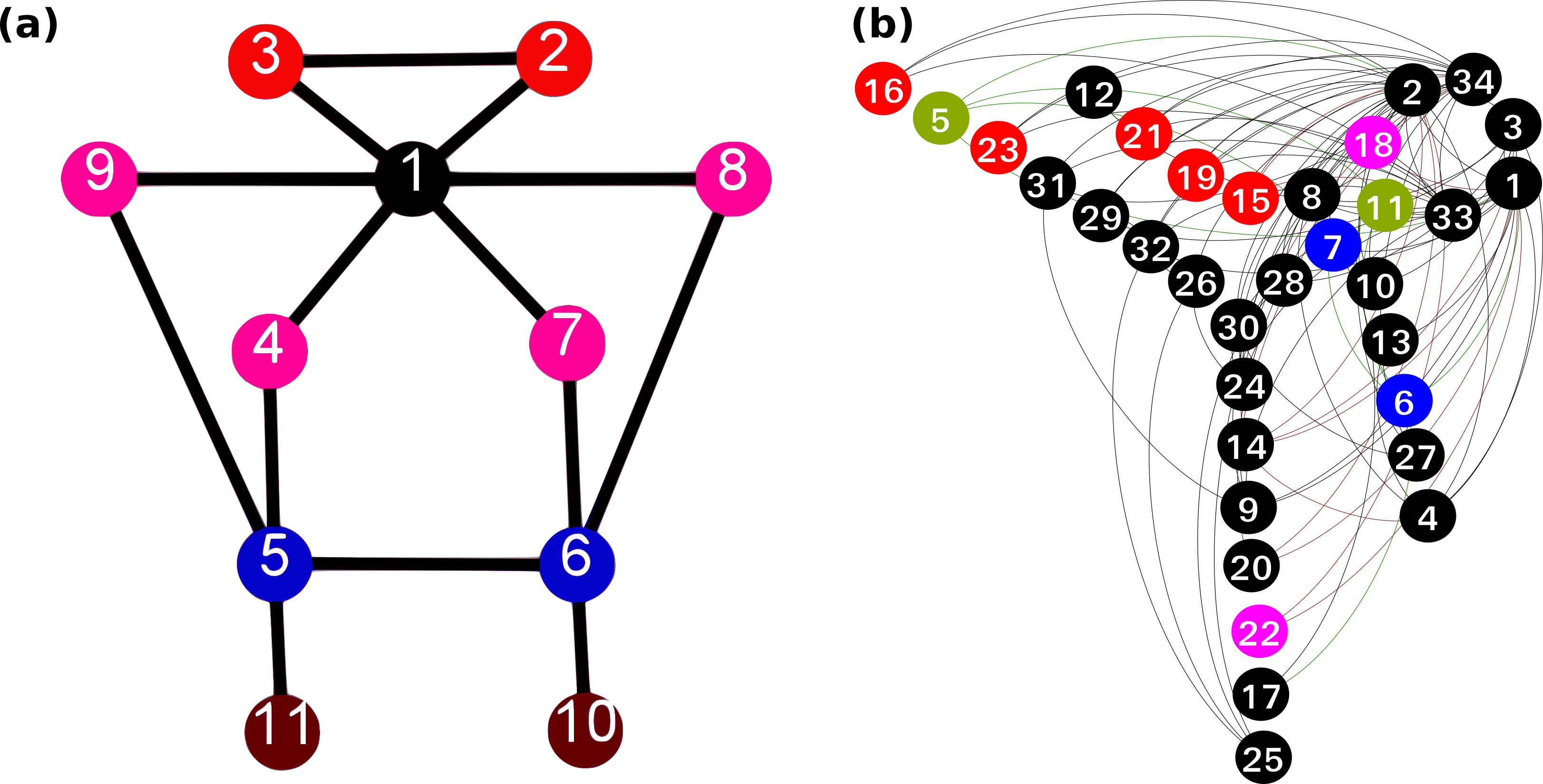
Figure 1: Symmetries and clusters in the considered networks. The graph in panel (a) is a synthetic network consisting of 11 nodes, and constructed in a way to display 4 sets of nontrivial clusters denoted by red, magenta, blue and brown color. The graph of panel (b) is, instead the well known Zachary karate club network Zachary (1977), and consists of 34 nodes. Symmetry analysis identifies again 4 clusters, denoted by magenta, red, blue, and green color. Nodes colored in black do not participate in any cluster.

Let us start by considering an undirected network $\mathcal{G}$ of size $\mathcal{N}$, and its adjacency matrix $\mathcal{A}=(A_{ij})_{\mathcal{N}\times\mathcal{N}}$. Mathematically, $\mathcal{G}$ is described as a connected graph $\mathcal{G}({\mathcal{V}},\mathcal{E})$, where ${\mathcal{V}}$ and $\mathcal{E}$ denote, respectively, the set of its vertices and edges, with $|{\mathcal{V}}|=\mathcal{N}$. Note that the edge set $\mathcal{E}$ consists of all ordered pairs $(i,j)\in{\mathcal{V}}\times{\mathcal{V}}$ such that the $i^{th}$ and $j^{th}$ nodes (vertices) are connected i.e. $\mathcal{E}\subseteq{\mathcal{V}}\times{\mathcal{V}}$.

Now, the graph $\mathcal{G}$ has a symmetry if and only if a bijective mapping $\Pi:{\mathcal{V}}\rightarrow{\mathcal{V}}$ exists that preserves the adjacency relation of $\mathcal{G}$, i.e. $\Pi$ is an automorphism for $\mathcal{G}$. In other words, a permutation matrix $\mathcal{P}=\mathcal{P}(\Pi)$ exists such that $\mathcal{P}\mathcal{A}(\mathcal{P})^{-1}=\mathcal{A}$. The collection of all such $\mathcal{P}$ forms the symmetry group $G$ of the graph $\mathcal{G}$ with respect to matrix multiplication operation. The action of the group $G$ on the set of nodes ${\mathcal{V}}$ divides it into disjoint invariant subsets which are called the clusters or orbits of the network. Symmetries are directly connected to CS  Nicosia et al. (2013): the nodes within an orbit will synchronize also in absence of GS for suitable values of the system’s parameters.

For instance, the graph in Fig. 1(a) is a synthetic network of $11$ nodes. There exists $15$ non-trivial bijective mappings [see Sec. II of our supplementary material (SM)] which preserves the adjacency relation, and which (along with the identity mapping) forms a group under matrix multiplication. One can then identify $4$ non-trivial orbits in this network: $(2,3:$ red nodes), $(5,6$ : blue nodes), $(9,8,4,7:$ magenta nodes), and $(10,11:$ brown nodes). Notice that the permutation of such nodes within an orbit preserves the connectivity pattern even when they are not neighbours to each other (such as nodes 9 and 8). The second network (Fig. 1(b), $\mathcal{N}=34$) is the celebrated Zachary karate club network Zachary (1977), and its group order (formed by $480$ elements) is increased by a factor $\sim 30$ as compared to the first case. Four non-trivial orbits/clusters can be identified from the group (see the SM for details on the generators and symmetry group of both networks). Depending on the structure of the graph, the number of symmetries can be of the order of a million or a billion times the network size (see Table 1 in Ref. Della Rossa et al. (2020)), thus making extremely complicated (if not impossible) the identification by classical methods of symmetry groups and orbits of large size networks.

The key question is then: can one extract the non-trivial clusters of an undirected graph without having to pass necessarily from the identification of the network’s symmetry groups? Our answer is affirmative, and we will show that an enormously easier and less demanding operation (the inspection of the elements of the graph’s EVC) is in fact sufficient for identifying the orbits and their member nodes. In the following, a proof is given which shows the direct relation between EVC and network clusters.

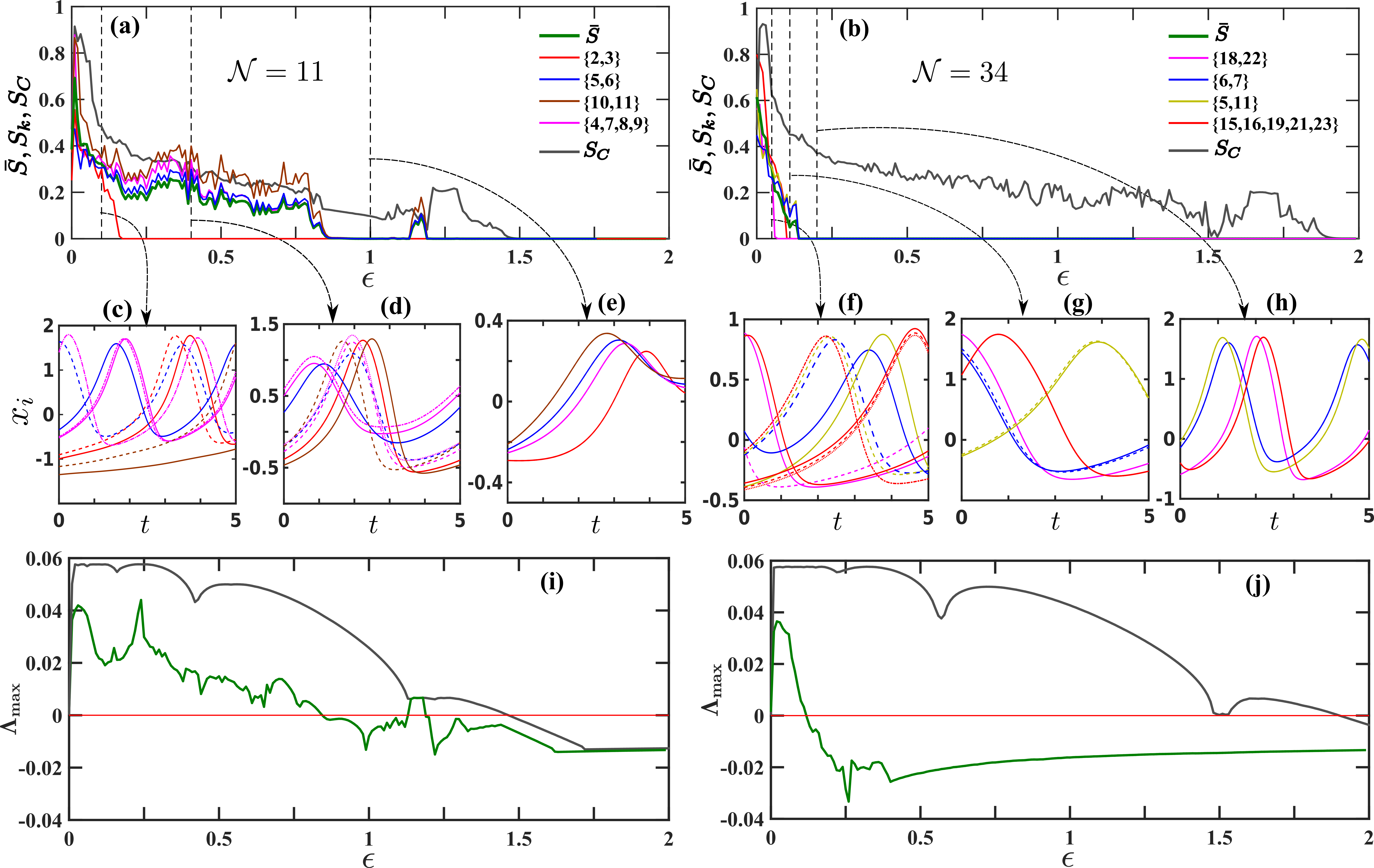
Figure 2: Synchronization errors and transverse Lyapunov exponents. (a,b): $\bar{S},S_{k},S_{C}$ (see text for definition) vs. $\epsilon$ for the two networks of Fig. (1). Color codes (reported in the legend of each panel) reflect the colors assigned to each cluster in Fig. (1). We have checked three coupling regimes (dashed vertical lines) for both networks. Panels (c-e) [(f-h)] report the time evolution of the nodes participating in each clusters of the first (the second) network, for the three values of $\epsilon$ marked with vertical dashed lines in panel (a) [(b)]. The full discussion on the different dynamical regimes observed is reported in the text. (i,j) The maximum Lyapunov exponents $\Lambda_{\rm max}$ transverse to the CCS (green) and the GS (black) manifolds vs. $\epsilon$.

Let $\mathbf{X}$ be the EVC, i.e. the eigen-vector of the adjacency matrix $\mathcal{A}$ corresponding its largest eigen-value $\lambda_{m}$. As $\mathcal{A}$ is symmetric, all its eigen-values are real, and the Perron-Frobenius theorem Perron (1907); Frobenius (1912) warrants that $\lambda_{m}$ is not degenerate, and that all the components of $\mathbf{X}$ are strictly positive. Then, one has $\mathcal{A}\mathbf{X}=\lambda_{m}\mathbf{X}$, and multiplying from left both sides by an element $\mathcal{P}$ of a symmetry group of $\mathcal{G}$ one gets $\mathcal{PA}\mathbf{X}=\lambda_{m}\mathcal{P}\mathbf{X}$, which implies $\mathcal{AP}\mathbf{X}=\lambda_{m}\mathcal{P}\mathbf{X}$ (because $\mathcal{AP=PA}$).

Assuming $\mathcal{P}\mathbf{X}=\mathbf{Y}$, one gets $\Rightarrow$ $\mathcal{A}\mathbf{Y}=\lambda_{m}\mathbf{Y}$. Hence, along with $\mathbf{X}$, also $\mathbf{Y}$ is an eigenvector of $\mathcal{A}$ corresponding to the same eigenvalue $\lambda_{m}$. Thus, the set $\{\mathbf{X},\mathbf{Y}\}$ must be linearly dependent, which implies the existence of a real number $c$ such that $\mathbf{Y}=c\mathbf{X}$, or $\mathcal{P}\mathbf{X}=c\mathbf{X}$. But now, since $\mathbf{Y}$ is nothing but a rearrangement of the elements of $\mathbf{X}$, the value of $c$ must be $1$. Therefore, one has

$$\mathcal{P}\mathbf{X}=\mathbf{X}.$$ (1)

Note that the relation (1) is true for all matrices $\mathcal{P}$ belonging to the symmetry group of $\mathcal{G}$, and it says that the EVC remains invariant under the action of such $\mathcal{P}$. Now since each cluster of $\mathcal{G}$ is mapped to itself by the action of all such $\mathcal{P}$, Eq. (1) can hold if and only if the components of $\mathbf{X}$ corresponding to the nodes of a cluster are equal. Moreover, the components of $\mathbf{X}$ corresponding to nodes of different clusters must be different. And this is because if they were equal then, apart from the symmetry group elements of the graph $\mathcal{G}$, there would be some other permutation matrices $\mathcal{P}^{\prime}$ for which $\mathcal{P}^{\prime}\mathbf{X}=\mathbf{X}$, and the action of those matrices on $\mathcal{A}$ would not satisfy $\mathcal{P^{\prime}A}=\mathcal{AP^{\prime}}$, with the immediate consequence that $\mathcal{P}^{\prime}\mathbf{X}(=\mathbf{X})$ would not be an eigen-vector of $\mathcal{A}$.

The simple and direct inspection of the EVC components allows, therefore, to identify the clusters of a network.

In what follows, we show that the clusters identified as the collections of those nodes displaying the same EVC value are exactly the ones where CS takes place, independently on the specific dynamical system implemented in the networks’ node. To do so, we consider a network of identical units, such that the uncoupled nodal dynamics is captured by $\dot{{\mathcal{X}}}=\mathbf{F}({\mathcal{X}})$, where dot denotes temporal derivative, ${\mathcal{X}}$ is a $p-$dimensional state vector, and ${\mathbf{F}}:{\mathbb{R}}^{p}\to{\mathbb{R}}^{p}$ is the flow function. The evolution equation for the $i^{th}$ unit ($i=1,...,N$) is therefore

$$\dot{\mathcal{X}}_{i} = \mathbf{F}({\mathcal{X}}_{i})+\mathbf{E}\sum_{j=1}^{\mathcal{N}}\mathcal{A}_{ij}\mathbf{Q}(\mathcal{X}_{j},\mathcal{X}_{i}),$$ (2)

where $\mathbf{E}=\rm{diag}(\epsilon_{1},\epsilon_{2},\dots,\epsilon_{p})$ is a $p\times p$ diagonal coupling matrix, and $\mathbf{Q}:{\mathbb{R}}^{2p}\to{\mathbb{R}}^{p}$ is a coupling function, which is here taken to be diffusive, i.e., $\mathbf{Q}(\mathcal{X}_{j},\mathcal{X}_{i})=(\mathcal{X}_{j}-\mathcal{X}_{i})$. The connectivity among the units is mapped into the $\mathcal{N}\times\mathcal{N}$ adjacency matrix $\mathcal{A}$. Under a suitable choice of $\mathbf{F}$ and $\mathbf{E}$, the system may exhibit CS, e.g. the nodes within each orbit will synchronize their evolution.

Let us first discuss the properties of CS in a network of neurons, the dynamic of whose action potential is given by the Hindmarsh-Rose (HR) model Hindmarsh and Rose (1982, 1984); Mishra et al. (2018); González-Miranda (2007). In the HR model, $p=3,\mathbf{E}=\rm{diag}(\epsilon,0,0),{\mathcal{X}}=(x,y,z)$, so that the evolution equation are ${\dot{x}}_{i}=y_{i}+bx_{i}^{2}-ex_{i}^{3}-z_{i}+I+\epsilon\sum_{i=1}^{\mathcal{N}}\mathcal{A}_{ij}(x_{j}-x_{i});\ {\dot{y}}_{i}=c-d{x}_{i}^{2}-y_{i};\ {\dot{z}}_{i}=rs(x_{i}-x_{R})-rz_{i}.$ Here, $x$ is the membrane potential in the axon, $y$ accounts for the fast ionic movement through membrane, and in the variable $z$ Hindmarsh and Rose (1984) a slow exchange of $Ca^{++}$ ions occurs due to the controlling parameter $r$. By properly setting the system’s parameters (the external currents $I$ and $r$), several complex spiking and bursting pattern arise. Here, we consider $e=c=1$, $b=2.6$, $d=5$, $s=4$, $r=0.01$, and $x_{R}=-1.6$. Furthermore, all units are kept in their oscillatory state ($I=4$), and an electrical diffusive coupling is introduced in the variable $x$. To monitor the onset of CS, we refer to the quantity $\bar{S}$ defined by $\bar{S}=\left\langle S_{k}\right\rangle$, where $\langle.\rangle$ denotes the average over the total number of non-trivial clusters, and $S_{k}$ is the time averaged root mean square deviation of the $k$th cluster defined as $S_{k}=\left\langle\left(\frac{1}{\mathcal{N}_{k}}\sum_{i\in v_{k}}(x_{i}-\bar{x}_{k})^{2}\right)^{1/2}\right\rangle_{t}$ (with $\mathcal{N}_{k}$ and $v_{k}$ being, respectively, the number and the set of nodes involved in the cluster $k$, and $\bar{x}_{k}$ denoting the average of the membrane potential of all axons within that cluster).

Figure 3: The Mackey-Glass system. (a): $\bar{S},S_{k},S_{C}$ (see text for definition) vs. $\epsilon$ for the network of Fig. 1(a). Color codes (reported in the legend) reflect the colors assigned to each cluster in Fig. 1. The black and green lines refer to $S_{c}$ and $\bar{S}$, respectively. (b-d): time series of each node forming clusters at three different values of $\epsilon$ (dashed vertical lines in panel (a)). Namely, $\epsilon=0.0121$ (b), $\epsilon=0.0394$ (c), and $\epsilon=0.0970$ (d).

Extracting the identical elements of the EVC from the adjacency matrix of the graph sketched in Fig. 1(a), it is fully confirmed that the network has four clusters. Namely, four nodes (marked by the magenta color in the Figure) participate in the largest orbital cluster, and the other three clusters are formed by two nodes each (marked by two blue nodes, two red nodes, and two brown nodes in the Figure). Fig. 2(a) reports the overall synchronization scenario, as the coupling strength $\epsilon$ is increased. Four distinct regimes can be identified. For $\epsilon<0.12$ the system stays in its fully incoherent state, which will be called from here on “no synchronization” (NS). A typical behavior of the system is shown at $\epsilon=0.1$ [first dashed vertical line from left of Fig. 2(a)] in Fig. 2(c). At $\epsilon\sim 0.12$, a first transition toward CS is seen, and a first cluster of nodes (nodes 2 and 3) synchronize. In Fig. 2(d), we report the time signals at $\epsilon=0.4$ [second dashed vertical line from left in Fig. 2(a)], and it is apparent that the thick red lines are indistinguishable, as the evolution of node 2 and 3 is synchronous. A second transition occurs at $\epsilon\sim 0.8$ towards Complete Cluster Synchronization (CCS). There, the other three clusters synchronize almost together. CCS then corresponds to $\bar{S}=0$, where all clusters are separately synchronized, i.e. each of them evolves within a separated (non synchronized) dynamical state, as shown in Fig. 2(e) for $\epsilon=1$ [third vertical line in Fig. 2(a)]. Eventually, the onset of GS, where $\left(S_{C}=\left\langle\sqrt{\left\langle(x_{i}-\bar{x})^{2}\right\rangle_{\mathcal{N}}}\,\right\rangle_{t}\right)=0$, occurs at $\epsilon\sim 1.5$, and the entire network synchronize. A similar scenario characterizes the dynamics of the Zachary karate club network, which has $\mathcal{N}=34$ nodes and $78$ links, and for which the EVC reveals again the presence of four nontrivial clusters [colored with magenta, blue, green, and red in Fig. 1(b)]. Precisely, in the NS regime ($\epsilon=0.05$, Fig. 2(b), left dashed vertical line) all nodes are unsynchronized (see Fig. 2(f) where all lines do not overlap). Increasing $\epsilon$ leads to CS. At the value of $\epsilon$ marked by the second dashed vertical line of Fig. 2(b), two clusters (magenta and red nodes) fire in unison, although with separated dynamics (Fig. 2(g)). Eventually, all the orbits are synchronized ($\bar{S}=0$), i.e., CCS appears at $\epsilon_{c}=0.14$. The time signals at $\epsilon=0.2$ are shown in Fig. 2(h). GS ($S_{c}=0$) appears here at a much higher coupling strength, as it can be seen in Fig. 2(b).

While assessment of stability of GS can be obtained from the Master Stability Function approach Pecora and Carroll (1998, 1990); Boccaletti et al. (2006), and of that of CS by a parallel analysis of synchronization in each cluster Pecora et al. (2014), the conditions for stability of CCS are reported in details in our SM. The maximum Lyapunov exponents $\Lambda_{\rm max}$ transverse to the CCS [green curves, from Eq. (3) of the SM] and to the GS [black curves, from Eq. (9) of the SM] manifolds are reported vs. $\epsilon$ in panels (i,j) of Fig. 2 for the two networks of Fig. 1. When compared with panels (a) and (b) of Fig. 2, there is a perfect correspondence between the vanishing of these two exponents and the transition points to CCS and GS, respectively. Notice that the stability of GS occurs always later than that of CCS.

Remarkably, all qualitative features of the synchronization scenario are independent on the specific dynamical system implemented in each of the network nodes. For instance, we considered a network of infinite-dimensional systems, the delayed Mackey-Glass systems Mackey and Glass (1977), which obeys $\dot{x}_{i}(t)=-0.1x_{i}(t)+0.2\frac{x_{i}(t-\tau)}{1+x_{i}(t-\tau)^{10}}+\epsilon\sum_{j=1}^{N}\mathcal{A}_{ij}\left[x_{j}(t)-x_{i}(t)\right]$, where $\tau=25$ is a delay time. Depending on the value of $\tau$ ($\tau>16.8$), each node evolves in a hyper-chaotic attractor, and the dimensionality of the phase space scales linearly with $\tau$ Doyne Farmer (1982). Results are reported in Figure 3 for the network of Fig. 1(a). In Fig. 3(a) it is clearly seen that the order at which each cluster synchronizes is exactly the same as the one shown in Fig. 2(a), i.e., the cluster marked in red 2,3 synchronizes first and the other three synchronize together at a higher value of the coupling strength. The overall scenario of synchronization is qualitatively the same as the one obtained for HR systems: a first transition from NS [Fig. 3(b)] to CS [Fig. 3(c)] is observed, but here the transition to CCS coincide with that to GS, and therefore the point at which all clusters synchronize is almost indistinguishable from that where network synchronization takes place [Fig. 3(d)].

In summary, we introduced a new framework for cluster analysis in undirected positive semi-definite networks, based on the proof of a direct relation between the components of the EVC and the membership of each clusters or orbits of the network. This substantially simplifies cluster analysis of networks of any size, and drastically reduces its computational cost. We further demonstrated that our analysis actually predicts the scenario of cluster synchronization supported by the network’s connectivity, independently on the specific dynamical system implemented in the network nodes. Thus, it is easy to expect that our approach will empower the study of symmetry related problems in all cases and circumstances in which it was prevented so far by the computational costs associated to the classical methods, such as, for instance, in epileptic seizures, power-grid failures, or emerging clustered behavior in social networks and/or brain dynamics.

C.H. is supported by INSPIRE-Faculty grant (Code: IFA17-PH193).

References

- Strogatz (2004) S. Strogatz, Sync: The emerging science of spontaneous order (Penguin UK, 2004).
- Boccaletti et al. (2006) S. Boccaletti, V. Latora, Y. Moreno, M. Chavez, and D.-U. Hwang, Physics Reports 424, 175 (2006).
- Dorfler and Bullo (2012) F. Dorfler and F. Bullo, SIAM Journal on Control and Optimization 50, 1616 (2012).
- Motter et al. (2013) A. E. Motter, S. A. Myers, M. Anghel, and T. Nishikawa, Nature Physics 9, 191 (2013).
- Ashwin et al. (2016) P. Ashwin, S. Coombes, and R. Nicks, The Journal of Mathematical Neuroscience 6, 2 (2016).
- Boccaletti et al. (2018) S. Boccaletti, A. N. Pisarchik, C. I. del Genio, and A. Amann, Synchronization: From Coupled Systems to Complex Networks (Cambridge University Press, 2018).
- Dahms et al. (2012) T. Dahms, J. Lehnert, and E. Schöll, Physical Review E 86, 016202 (2012).
- Skardal et al. (2011) P. S. Skardal, E. Ott, and J. G. Restrepo, Physical Review E 84, 036208 (2011).
- Nicosia et al. (2013) V. Nicosia, M. Valencia, M. Chavez, A. Díaz-Guilera, and V. Latora, Physical Review Letters 110, 174102 (2013).
- Sorrentino and Ott (2007) F. Sorrentino and E. Ott, Physical Review E 76, 056114 (2007).
- Williams et al. (2013) C. R. Williams, T. E. Murphy, R. Roy, F. Sorrentino, T. Dahms, and E. Schöll, Physical Review Letters 110, 064104 (2013).
- Pecora et al. (2014) L. M. Pecora, F. Sorrentino, A. M. Hagerstrom, T. E. Murphy, and R. Roy, Nature Communications 5, 4079 (2014).
- Sorrentino et al. (2016) F. Sorrentino, L. M. Pecora, A. M. Hagerstrom, T. E. Murphy, and R. Roy, Science Advances 2, e1501737 (2016).
- Lodi et al. (2020) M. Lodi, F. Della Rossa, F. Sorrentino, and M. Storace, Scientific Reports 10, 1 (2020).
- Bergner et al. (2012) A. Bergner, M. Frasca, G. Sciuto, A. Buscarino, E. J. Ngamga, L. Fortuna, and J. Kurths, Physical Review E 85, 026208 (2012).
- Sorrentino and Pecora (2016) F. Sorrentino and L. Pecora, Chaos: An Interdisciplinary Journal of Nonlinear Science 26, 094823 (2016).
- Gambuzza and Frasca (2019) L. V. Gambuzza and M. Frasca, Automatica 100, 212 (2019).
- Siddique et al. (2018) A. B. Siddique, L. Pecora, J. D. Hart, and F. Sorrentino, Physical Review E 97, 042217 (2018).
- Wang et al. (2019) Y. Wang, L. Wang, H. Fan, and X. Wang, Chaos: An Interdisciplinary Journal of Nonlinear Science 29, 093118 (2019).
- Karakaya et al. (2019) B. Karakaya, L. Minati, L. V. Gambuzza, and M. Frasca, Physical Review E 99, 052301 (2019).
- Zhang et al. (2017) L. Zhang, A. E. Motter, and T. Nishikawa, Physical Review Letters 118, 174102 (2017).
- Cho et al. (2017) Y. S. Cho, T. Nishikawa, and A. E. Motter, Physical Review Letters 119, 084101 (2017).
- Della Rossa et al. (2020) F. Della Rossa, L. Pecora, K. Blaha, A. Shirin, I. Klickstein, and F. Sorrentino, Nature Communications 11, 1 (2020).
- Sorrentino et al. (2020) F. Sorrentino, L. M. Pecora, and L. Trajkovic, IEEE Transactions on Network Science and Engineering (2020).
- Pradhan et al. (2020) P. Pradhan, C. Angeliya, and S. Jalan, Physica A: Statistical Mechanics and its Applications , 124169 (2020).
- Newman (2010) M. Newman, Networks: an introduction (Oxford University Press, 2010).
- Zachary (1977) W. W. Zachary, Journal of Anthropological Research 33, 452 (1977).
- Perron (1907) O. Perron, Mathematische Annalen 64, 248 (1907).
- Frobenius (1912) F. Frobenius, Sitzungsberichte Akad. Wiss. Berlin 26, 456 (1912).
- Hindmarsh and Rose (1982) J. Hindmarsh and R. Rose, Nature 296, 162 (1982).
- Hindmarsh and Rose (1984) J. Hindmarsh and R. Rose, Proceedings of the Royal Society of London. Series B. Biological Sciences 221, 87 (1984).
- Mishra et al. (2018) A. Mishra, S. Saha, M. Vigneshwaran, P. Pal, T. Kapitaniak, and S. K. Dana, Physical Review E 97, 062311 (2018).
- González-Miranda (2007) J. González-Miranda, International Journal of Bifurcation and Chaos 17, 3071 (2007).
- Pecora and Carroll (1998) L. M. Pecora and T. L. Carroll, Physical Review Letters 80, 2109 (1998).
- Pecora and Carroll (1990) L. M. Pecora and T. L. Carroll, Physical Review Letters 64, 821 (1990).
- Mackey and Glass (1977) M. Mackey and L. Glass, Science 197, 287 (1977).
- Doyne Farmer (1982) J. Doyne Farmer, Physica D: Nonlinear Phenomena 4, 366 (1982).