Tight factorizations of girth--regular graphs
Italo J. Dejter
University of Puerto Rico
Rio Piedras, PR 00936-8377
italo.dejter@gmail.com
Abstract
Girth-regular graphs with equal girth, regular degree and chromatic index are studied for the determination of 1-factorizations with each 1-factor intersecting every girth cycle. Applications to hamiltonian decomposability and to 3-dimensional geometry are given. Applications are suggested for priority assignment and optimization problems.
1 Introduction
Let . Given a finite graph with girth , we inquire whether assigning colors to the edges of properly (i.e., no two adjacent edges of equal color in ) can be performed so that each -cycle of has a bijection from the edges of to the colors. Such an inquiry is applicable to managerial situations in which a number of agents must participate in committees around round tables, with stools about each table. A roster of tasks is handed to each agent at each round table, and such an agent is assigned each of the tasks but at pairwise different tables. This can be interpreted as a 2-way (vertex incidence versus girth-cycle membership) problem of sorting the colors according to some prioritization hierarchy. This way, an assignment problem is conceived, with potential applications in optimization and decision making. We pass to formalize such ideas.
Let be a finite connected -regular simple graph with chromatic index . Let be the girth of . We say that is a -tight graph if . In each -tight graph , it makes sense to look for a proper edge-coloring via colors, each girth cycle colored via a bijection between the cycle edges and the colors they are assigned, precisely colors. We will say that such a coloring is an edge-girth coloring of and, in such a case, that is edge-girth chromatic, or egc for short.
We focus on -tight -regular graphs that are girth-regular, a concept whose definition in [17] we adapt as follow. Let one such graph. Let be the set of edges incident in to a vertex . Let be the number of -cycles containing an edge , for . Assume . Let the signature of be the -tuple . The graph is said to be girth-regular if all its vertices have a common signature. In such a case, the signature of any vertex of is said to be the signature of .
In this work, girth-regular graphs that are -tight will be said to be girth--regular graphs as well as -graphs, or -graphs, if no confusion arises, where . In this notation, a prefix
with iff may be abbreviated as , where superscripts equal to 1 may be omitted (e.g., abbreviates to ). So, the prefixes will include and further be denoted as follows:
- (i)
- (ii)
- (iii)
- (iv)
- (v)
Extending this context, girth-regular graphs of regular degree and girth larger than will be said to be -graphs, or improper -graphs.
Edge-girth colorings of -graphs are equivalent to 1-factorizations [22] such that the cardinality of the intersection of each 1-factor with each girth cycle is 1. These factorizations are said to be tight, and the resulting colored girth cycles, are said to be tightly colored. Note a with a tight factorization is egc. Unions of pairs of 1-factors of such graphs are treated in Section 7 for their hamiltonian decomposability, (Corollary 36). Applications to Möbius-strip compounds and hollow-triangle polylinks are found in Section 8.
2 Egc girth-3-regular graphs
Theorem 1.
[17] There is only one -graph with , namely . Moreover, is egc. All other proper -graphs are -graphs, but not necessarily egc.
Proof.
Remark 2.
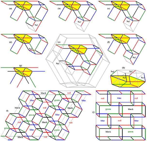
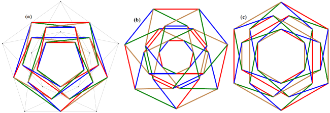
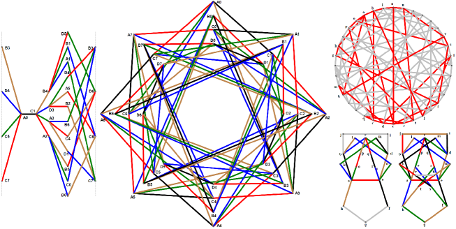
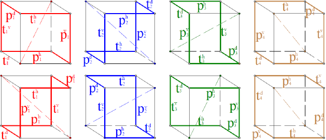
In order to determine which -graphs are egc, let be a finite undirected loopless cubic multigraph. Let with and . Then, determines two arcs (that is, ordered pairs of end-vertices of ) denoted and (if the girth of is larger than 2, then is a simple graph, a particular case of multigraph). The following definition is an adaptation of a case of the definition of generalized truncation in [10]. Let denote the set of arcs of . A vertex-neighborhood labeling of is a function such that for each the restriction of to the set of arcs leaving is a bijection. For our purposes, we require , with , so that each is assigned a well-defined color from the color set . This yields a 1-factorization of with three 1-factors that we can call for respective color 1, 2, 3, with being the disjoint union . For the sake of examples in Fig. 1, to be presented below, let colors 1, 2 and 3 be taken as red, blue and green, respectively.
Let be the triangle graph with vertex set . The triangle-replaced graph of with respect to has vertex set and edge set
Note that is a -graph. We will refer to the edges of the form ( as -edges or triangle edges, and to the edges , , as -edges or non-triangle edges. Observe that a -edge is incident only to -edges and that each vertex of is incident to precisely one -edge. This yields the following.
Observation 3.
[10] Let be a finite undirected cubic multigraph of girth . Then, for any vertex-neighborhood labeling of , the shortest cycle in the triangle-replaced graph containing a -edge is of length at least .
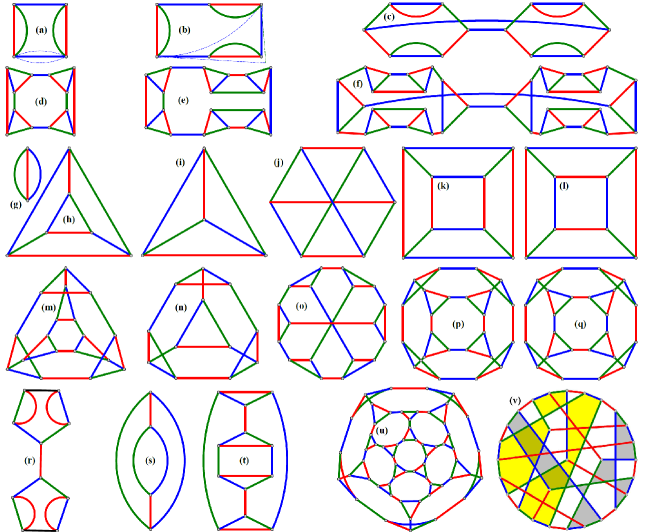
We say that is a generalized snark if its chromatic index is larger than 3. Two examples of generalized snark are: (i) the Petersen graph and (ii) the multigraph obtained by joining two -cycles () via an extra-edge (a bridge between the two -cycles) and adding parallel edges to each of the two -cycles so that the resulting multigraph is cubic, see Fig. 1(r) for . The triangle-replaced graph of a generalized snark will also be said to be a generalized snark. This denomination will also be used for the triangle-replaced graphs of , for , etc. In addition, we will say that is snarkless if it is not a generalized snark. Clearly, is snarkless.
Vertex-neighborhood labelings for the examples of below, represented in Fig. 1, have the elements 1, 2 and 3 of interpreted respectively as edge colors red, blue and green. Now, the smallest snarkless multigraphs are:
- (A)
- (B)
Given a snarkless , a new snarkless multigraph is obtained from by replacing any edge with end-vertices say , by the submultigraph resulting as the union of a path and an extra edge with end-vertices . For example, in Fig. 1(g) as in Fig. 1(s) and in Fig. 1(t). Using this replacement of an edge by the said submultigraph, one can transform the submultigraph with the enclosed blue edge in item (B), above, into a as in Fig. 1(b), with in Fig. 1(e); or with the four red and green edges into a as in Fig. 1(c), with in Fig. 1(f).
The triangle-replaced graph of any snarkless -graph , either proper or improper, with , yields an egc -graph, illustrated via the four graphs in Fig. 1(h–k), namely and (the 3-cube graph), onto the four -graphs in Fig. 1(m–p). This raises the observation that non-equivalent 1-factorizations of an -graph , like in Fig. 1(k–l) for , result in non-equivalent 1-factorizations of , represented in this case on in Fig. 1(p–q). This leads to the final assertion in Theorem 4, below.
Fig. 1(u) is the egc -graph given by for the dodecahedral graph , in which the union of any two edge-disjoint 1-factors of a 1-factorization of yields a Hamilton cycle. In contrast, the Coxeter graph in Fig. 1(v) is non-hamiltonian, but the union of any two of its (edge-disjoint) 1-factors is the disjoint union of two 14-cycles, whose apparent interiors are shaded yellow and light gray in the figure. Thus, is an egc -graph.
Theorem 4.
A -graph is egc if and only if is the triangle-replaced graph of a snarkless . Moreover, non-equivalent 1-factorizations of such result in corresponding non-equivalent 1-factorizations of .
Proof.
There are two types of edges in a -graph , namely the triangle edges (those belonging to some triangle of ) and the remaining non-triangle edges. Each vertex of is incident to a unique non-triangle edge and is nonadjacent to a unique edge (opposite to ) in the sole triangle of to which belongs. In any 1-factorization of , both and belong to the same factor (). Moreover, each edge of (where ) belongs solely to corresponding triangles and with opposite edges and . Clearly, with equality given precisely when is the triangular prism in Fig. 1(h).
We will define an inverse operator of that applies to each egc -graph . Given one such , contracting simultaneously all the triangles of consists in removing the edges of those and then identifying the vertices of each into a corresponding single vertex , where , for , has its unique incident non-triangle edge of with color . This is done so that whenever two triangles and have respective vertices and adjacent in (), then and the edge of is removed and replaced by a new edge . The result of these simultaneous triangle contractions is a multigraph with each incident to three edges of , one per each color in . The ensuing edge coloring in corresponds to a vertex-neighborhood labeling of , from which it follows that is the triangle-replaced graph of with respect to , that is: . This establishes an identification of and so that the triangle-edges of are the -edges of , and the non-triangle edges are the -edges of . This implies the main assertion of the statement of the theorem. ∎
3 Egc girth-4-regular graphs
Remark 5.
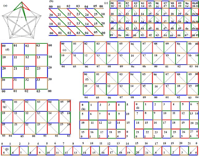
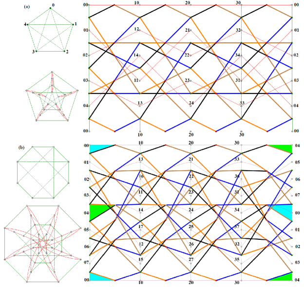
In this section and in Section 4, we consider -graphs with . Many such graphs are toroidal and obtained from the square tessellation denoted by its Schläfli symbol . Let be the group of translations of the plane that preserve such tessellation . Then, is isomorphic to and acts transitively on the vertices of . If is a subgroup of finite index in , then is a finite map of type on the torus, and every such map arises this way ([24], Section 6). A symmetry of acts as a symmetry of if and only if normalizes . Every such has symmetry group transitive on vertices, horizontal edges and vertical edges. Moreover, for each edge of , there is a symmetry that reverses . The tessellation may be considered as a lattice, so it has a fundamental region [4, 5]. Such region will be called a cutout and be given by a rectangle squares wide and squares high, with the left and right edges identified by parallel translation in order to get a toroidal embedding of , and the bottom edges identified with the top edges after a shift of squares to the right, as in Fig. 6 of [24]. A toroidal graph with such a cutout will be denoted . While the aim of [18, 19, 24] is the study of edge-transitive graphs, we find 1-factorizations of -tight graphs in graphs of a more ample nature. Our notation for the vertices of those cutouts will be , or if no confusion arises, where and , as in the examples of tight factorizations in Fig. 2(d–j). For as in Fig. 2(d-g), the notation arises from the fact that can be considered as the undirected Cayley graph of the direct-sum group with generator set formed by for horizontal left-to-right arcs and for vertical up-to-down arcs. In case (Fig. 2(c, h–j)), we simplify notation by writing , instead of or . In Fig. 2, edge colors are encoded by numbers as follows: 1 for red, 2 for blue, 3 for green and 4 for hazel. (Thin and dashed diagonals of squares are to used in the proof of Theorem 10).
Remark 6.
If a fundamental region of as in Remark 5 is identified in reverse on a pair of opposite sides, and directly on the other pair, we get a Klein bottle [23]. There are egc-graphs that are skeletons of a -tessellation of , for example in Fig. 2(b), whose embedding into has corresponding cutout that can be obtained from the one of above (with ) first by replacing the vertical edges by corresponding square-face diagonals, while keeping the horizontal edges (so the new faces are lozenge rhombi), and second by identifying the horizontal top and bottom borders of the original cutouts, as well as the left and right borders, these with reverse orientations, with the resulting -embedding that we will denote . Then, the example of Fig. 2(b) is in . If is identified in reverse on both pairs of opposite sides, a projective-planar graph is obtained. This can be ruled out because -tessellations only exist on surfaces with Euler characteristic 0.
Remark 7.
Let . The -cube graph has as vertices the -tuples with entries in and edges only between vertices at unit Hamming distance. In Subsection 3.1, we consider the 4-cube graph . Other -graphs with and that are not prisms of -graphs are:
-
(i)
the bipartite complement of the Heawood graph, in Subsection 3.3;
-
(ii)
the subdivided double [18, 24] of a -regular graph is the bipartite graph with vertex set and an edge between vertices and whenever is incident to in ; [18, Lemma 4.2] asserts that if is 4-regular and arc-transitive, then is 4-regular and semisymmetric; for example, the Folkman graph (Fig. 2(a)) is the subdivided double of the complete graph ;
-
(iii)
the circulant graphs, i.e. the Cayley graphs of the cyclic group () with generating sets , where , and ; most of these are -graphs (assuming even, otherwise chromatic index is not 4), with additional cycles appearing whenever a congruence holds, (e.g., is a -graph, is a -graph, is a -graph and is a -graph); however, such graphs can always be seen as toroidal graphs;
-
(iv)
the wreath graphs (), i.e. lexicographic products of an -cycle and the complement of ; these are -graphs; ( is a -graph).
Remark 8.
If an -graph as in Remark 7 contains a subgraph guaranteeing that is not an egc-graph, then is said to be an egc-obstruction. A subgraph is an egc-obstruction for a girth-4-regular graph , since each of the proper edge-colorings of contains a quadrangle of with only two colors. In Fig. 2(a), one such graph , namely the Folkman graph is presented with a subgraph formed by a green quadrangle and a red 2-path. and also have obstruction isomorphic to .
Lemma 9.
A sufficient condition for an -graph with () to be egc is existence of 2-factorization of such that each 2-factor ():
-
1.
is the disjoint union of even-length cycles; and
-
2.
has an even-length cycle as in item 1, for each 4-cycle of , sharing with exactly two consecutive edges.
Proof.
A 1-factorization of via colors 1 and 2 and a 1-factorization of via colors 3 and 4 exist and form a tight 1-factorization of . ∎
Theorem 10.
The following -, - and -graphs exist, and are egc or not, as indicated:
-
1.
-graphs comprising the:
-
(a)
bipartite complement of the Heawood graph, which is not egc, (Subsection 3.3);
-
(b)
4-regular subdivided doubles of -regular graphs , which are not egc;
- (c)
-
(a)
- 2.
- 3.
A cycle of a graph as in Remarks 5-6 is said to be 1-zigzagging if it is formed by alternate horizontal and non-horizontal (i.e., all vertical or all -tilted) edges. A 2-factor of is said to be 1-zigzagging if its composing cycles are 1-zigzagging. A 2-factorization of is said to be 1-zigzagging if its composing 2-factors are 1-zigzagging.
Proof.
We pass to analyze the different items composing the statement of Theorem 10.
Items 1 and 2: Item 1() is proved in Subsection 3.3. The graphs of item 1() have egc-obstructions (see Remark 8) formed by three edge-disjoint paths of length 2 between two nonadjacent vertices, e.g., in Fig. 2(a), with egc-obstruction formed by four green edges and two red edges. Items 1() and 2() are proved in Subsection 3.2, Remark 11; (see also Fig. 2(d)). Item 2() is proved by concatenating copies of , as in Fig. 2(d).
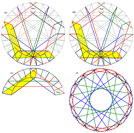
Item 3: Lemma 9 applies to each as in Remarks 5-6 via the 1-zigzagging 2-factorization , which contains its 2-factors having exactly two consecutive edges in common with each 4-cycle, as shown in Fig. 2(e,f,g,j,b,c). In items 3(–), the non-egc cases indicated via “” include those not satisfying the sufficient condition of Lemma 9, because such condition becomes also necessary for each arising from a toroidal or Klein-bottle cutout as in Remarks 5– 6. Moreover, all the 1-zigzagging cycles in have even length and share two consecutive edges with each 4-cycle precisely where indicated via “” in items 3(–). Furthermore, in Fig. 2(e,f,g,j), the thin diagonals separate those pairs of consecutive edges (for the 2-factorization ), while the dashed ones do the same for the 2-factorization . In addition, note the exclusion in item 3() of the cases and those for which , and in item 3() the case . In item 3(), note the lower bound for , due to being a -graph but not egc. For item 3(), the case is covered in item 2().
For the cases of Klein-bottle graphs in item 3(), there are two different color patterns, the first one, exemplified in Fig. 2(b), valid for and the second one further restricted to having , with more than two colors on each horizontal line. Note the exclusion of the cases (), for they are not girth-regular. ∎
The egc-cases of Theorem 10 item 3 are exemplified respectively in Fig. 2(e,f,g,j,b,c), characterized by having cycles with blue-hazel horizontal edges and cycles with red-green non-horizontal edges. However, transposing the two colors in 1-zigzagging cycles of 2-factors in 2-factorizations , or yield tight factorizations with horizontal cycles colored with more than 2 colors.
3.1 The 4-cube as a twice-egc girth-4-regular graph
Consider the three mutually orthogonal Latin squares of order 4, or MOLS(4) [3] contained as the second, third and fourth rows in the following compound matrix:
| (6) |
where for us row and column headings will stand for the following 4-tuples:
| (9) |
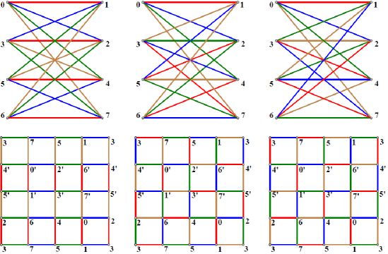
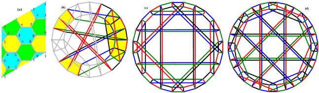
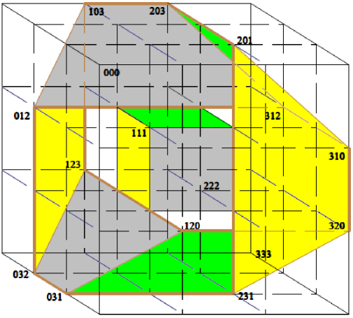
Based on display (6), the top of Fig. 3 contains three copies of properly colored in a mutually-orthogonal way, where colors are numbered as established in Remark 5. Letting be the canonical projection map of seen as a double covering of obtained by identifying the pairs of antipodal vertices of , these vertices denoted as in display (9), note that in the bottom of Fig. 3 corresponding copies of the colored inverse images of the three mentioned copies of are depicted. The leftmost copy of in Fig. 3 has color attributed precisely to those edges parallel to the coordinate direction, for . This constitutes a 1-factorization of . On the other hand, the center and rightmost copies of in the figure determine 1-factorizations and of for which each girth cycle of intersects every composing 1-factor of , where and 1 (red), 2 (blue), 3 (green), 4 (hazel).
For each edge of , we say that has -color if . Then, each 4-cycle of has opposite edges with a common 0-color in , with a total of two (nonadjacent) 0-colors in per 4-cycle, say 0-colors , with , so one such 4-cycle can be expressed as . On the other hand, the 4-cycles of use all four -colors 1,2,3,4, once each, for .
There are twenty-four 4-cycles in , six of each of the 0-color 4-cycles expressed in the first two columns of the following array, with two complementary 0-color 4-cycles per row. On the other hand, the third and fourth columns here contain respectively the 1-color and 2-color 4-cycles corresponding to the 0-color 4-cycles in the first two columns:
| (13) |
3.2 Toroidal representation tables
Remark 11.
The triple array in Table 1 presents () in schematic representations of , where stands for a vertex of and stands for an -color 4-cycle. This table guarantees Theorem 10 item 3() via the last two columns of color quadruples in display (13), because the four colors are employed on the edges of each 4-cycle:
-
(a)
either as horizontal or vertical color quadruples (as in display 13) alternated with the symbols that represent the vertices of ;
-
(b)
or as quadruples around the symbols representing the other 4-cycles.
By associating the oriented quadruple (1,3,2,4) (resp. (3,4,1,2)) of successive edge colors on the left-to-right and the downward (resp. the right-to-left and the downward) straight paths in (resp. ), situations that we indicate by “” (resp. “”), a complete invariant for (resp. ) is obtained that we denote by combining between square brackets the just presented notations:
This invariant distinguishes and from each other and is generalized for the toroidal graphs in Theorem 10, as we will see below in this subsection.
Table 1 is also presented to establish similar patterns, like in Table 2, allowing in a likewise manner to guarantee Theorem 10 item 2(). We say that
-
1.
has -zigzags if any 1-zigzagging path obtained by walking left, down, left, down and so on, alternates either colors 1 and 2, or colors 3 and 4;
-
2.
has -zigzags if any 2-zigzagging path obtained by walking right, right, down, down and so on, alternates either colors 1 and 3, or colors 2 and 4;
-
3.
has -zigzags if any 2-zigzagging path obtained by walking left, left, down, down and so on, either alternates colors 1 and 2, or colors 3 and 4;
-
4.
has -zigzags if any 1-zigzagging path obtained by walking right, down, right, down and so on, either alternates colors 1 and 3, or colors 2 and 4.
A representation as in Table 1 may be used for the graphs in items 1() and 2 of Theorem 10. For example, the cases and in Fig. 2(h–i) are representable as in Table 2, where, instead of standing for each vertex, we set the vertex notation of Fig. 2(h–i). Here the four colors are indicated as in Fig. 2(d–j) and Subsection 3.1. To distinguish the two cases in Table 2, note that the 4-cycles of (resp. ) have the 2-factors by color pairs and descending in zigzag from right to left (resp. left to right), by alternate vector displacements (resp. ) for colors 1 and 3, and for colors 2 and 4. Generalizing and using the invariant notation of Remark 11, we can say that the egc graphs in item 2(b) of Theorem 10 are as follows:
-
1.
for has invariant ;
-
2.
for has invariant .
3.3 The bipartite complement of the Heawood graph
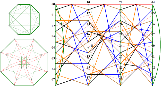
The bipartite complement of the Heawood-graph, with vertex set , , is depicted on the upper left of Fig. 4; its edges , , and , for , will be denoted , , and , respectively, where addition is taken. This yields the twenty-eight edges of as arcs from to vertices. They form twenty-one 4-cycles () expressed, by omitting the signs , as in Table 3.
This way, , , and , . We show there is no proper edge coloring of that is tight on every 4-cycle. To prove this, we recur to the bipartite graph whose parts and are respectively the twenty-eight edges of and the twenty-one 4-cycles of , with adjacency between an edge of and a 4-cycle of whenever passes through ; is represented in Fig. 4(b) with written as (). A tight factorization of would be equivalent to a 4-coloring of that is monochromatic on each vertex of but covering the four colors at the edges incident to each vertex of . We begin by coloring the edges incident to vertices respectively with colors black, red, blue and green. This forces the coloring of the subgraph of in the lower left of Fig. 4. By transferring this coloring to the representation of on the right of Fig. 4, as shown, it is verified that vertex 15 on the bottom of the representation does not admit properly any of the four used colors.
4 Prisms of types 4443, 3221 and 3221
Given a graph , the prism graph of is the graph cartesian product . The cases of -graphs with , apart from those treated in Section 3, are the prisms of -graphs . It is easy to see that there is no egc graph if is odd.
Conjecture 12.
Graphs with signatures and are not egc.
Example 13.
Conjecture 12 is sustained by the exhaustive partial colorings of the prisms of the 24-vertex truncated octahedral graph [8, pp. 79–86] in Fig. 5(a–g) and of the 6-vertex Thomsen graph [7] in Fig. 5(h), which are respectively a -graph and a -graph, with the incidental obstructions indicated by a notification ”No!” in each case. Such exhaustive partial colorings can be found similarly for example in the 120-vertex truncated-icosidodecahedral graph [8, pp. 97–99].
Remark 14.
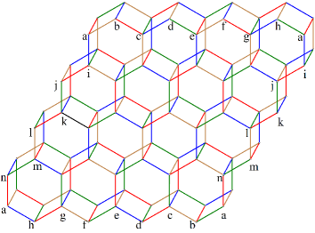
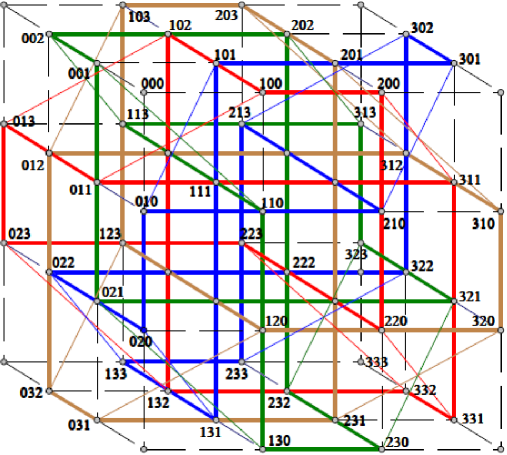
A -graph , where is a toroidal quotient graph of the hexagonal tessellation [4, 5] (i.e. the tiling of the plane with Schläfli symbol ), may be an egc -graph. This is exemplified in Fig. 5(i–j), namely for the prisms of the 24-vertex star graph (with twelve girth 6-cycles) [9] and a 16-vertex graph (with just eight girth 6-cycles). But cannot be the Pappus graph. Let us see why. A cutout in this case, as in Fig. 6(a) (with octodecimal vertex notation and proper face coloring) contains nine hexagonal tiles. In order to use the specified coloring to guarantee the existence of an egc-graph, the “period” employed when moving from any particular vertex of a cutout in any of the three directions perpendicular to the edges of the tessellation – i.e., the number of tiles met until a similar vertex in a cutout adjacent to is reached – must be even, but 9 is odd, leading to a contradiction.
Remark 15.
In the setting of Remark 14, by considering the junction of three hexagonal prisms , it is seen that in any such (), two edges not belonging to a hexagon can only be of the same color if their endpoints are antipodal in the two hexagons of . Up to automorphism and permutation of colors, this allows for two distinct colorings of the hexagonal prisms:
-
1.
the one as in both instances of Fig. 5(i–j) (with one color appearing on six edges and the remaining four colors appearing each on four edges), and
-
2.
one with two colors appearing each on five edges and the other two colors appearing each on four edges.
See Fig. 7, depicting a cutout of an egc-graph on the Klein bottle, namely an edge-girth coloring of the prism of [23] on the Klein bottle. In Fig. 7, the colorings of the hexagonal prisms in which one color appears six times only occur in the first row, and no edge-girth coloring of this graph is possible if only such colorings are used. Computational evidence has been obtained that gives support to the following conjectures.
Conjecture 16.
The condition of even periods in Remark 14 is sufficient for the case of prisms of hexagonal tessellations of the torus.
Conjecture 17.
Example 18.
Conjecture 17 is sustained by the prism cutout in Fig. 7, showing an edge-girth coloring of the prism of [23] on the Klein bottle. Note that the colorings of the hexagonal prisms in which one color appears six times only occur in the first row, and no edge-girth coloring of this graph is possible if only such colorings are used.
Example 19.
In Fig. 6(b), the prism of the Desargues graph on twenty vertices is shown non-egc via obstructions by pairs of forced “long” parallel red edges. However, in Fig. 6(c–d) the Nauru and Dyck graphs on twenty-four and thirty-two vertices, respectively, are shown to have their prisms as egc graphs by means of corresponding tight factorizations.
Example 20.
For the case , let us consider to be the Tutte 8-cage on 30 vertices. Fig. 8(a–c) shows why its -graph prism is not egc, with five 8-cycle prisms in (presented cyclically mod 5), each of whose vertices should have its four incident edges colored differently. In fact, Fig. 8(a–c) presents exhaustively without loss of generality partial edge-colorings in , with copies of edge-colored accordingly and notification “No!” if an obstruction to edge-coloring continuation appears.
On the other hand, Table 4 uses the notation of Table 1 in representing a coloring of the union of almost four (namely ) contiguous 8-cycle prisms () and the resulting forced colors for the departing edges away from . In Table 4, the middle row sequence, call it , (obtained by disregarding the symbols “”, or replacing them by commas) represents the subsequences of colors of the edges in the prisms , namely the subsequences , , and . Here, the last two terms of each coincide (i.e. are shared) with the first two terms of its subsequent , where the last 6-term subsequence is completed to by adding the first two terms of , so may be considered as the next after the last (and explaining the fraction mentioned above). This suggest that can be concatenated with itself a number of times to close a -cycle of colors for the edges of a Hamilton-cycle (of ) prism which may be completed to an egc graph by means of the following considerations. (An adequately colored graph is obtained from Fig. 8(d) by adding a suitable colored outer cycle, missing in the figure).
On the top and bottom rows of Table 4, the colors 1, 2, 3 and 4 with a bar on top are those of the “long” edges in the four prisms that close the two 8-cycles in each . The remaining (non-barred) colors suggest that the corresponding edges form external 4-cycles that may be joined with to form a as desired. The “even longer” edges of these external 4-cycles must be set to form (with two edges of the form ) new 4-cycles and can be selected to form the desired by taking the number of concatenated copies of to be , so that . The two columns in Table 4 whose transpose rows are “” and “”, namely the third leftmost and seventh rightmost -free columns, integrate one such 4-cycle. The leftmost third, fourth, fifth and sixth columns are paired this way with the rightmost seventh, eighth, ninth and tenth columns, but the last three pairs must be paired with similar columns in the second, third and fourth version of Table 4 (for indices of copies of , if we agree that the leftmost third and rightmost seventh columns above are both for and ). The same treatment can be set from the leftmost ninth, tenth, eleventh and twelveth respectively to the rightmost first, second, third and fourth columns, which also correspond in pairs that form again “long” 4-cycles.
Theorem 21.
For each , there is an egc -graph with edges as a prism of a hamiltonian cubic graph on vertices based on contiguous copies of the edge-colored subgraph in Table 4. However, the Tutte 8-cage is a non-egc -graph.
Proof.
The argument above the statement can be completed for the case . By concatenating the graph from Table 4 any multiple of times, one extends the construction. ∎
Remark 22.
The cubic vertex-transitive graphs on less than one hundred vertices with girth 10 and that have egc prisms are in the notation of [16]:
CubicVT[80,30], CubicVT[96,34], CubicVT[96,49], CubicVT[96,50] and CubicVT[96,62].
5 Egc 1111-graphs
A construction [24] of -graphs, also called girth-tight [18], proceeds as follows. Let be 4-regular and let be a partition of into cycles. The pair is a cycle decomposition of . Two edges of are opposite at vertex if both are incident to and belong to the same element of . The partial line graph of is the graph with the edges of as vertices, and any two such vertices adjacent if they share, as edges, a vertex of and are not opposite at that vertex. A cycle in is -alternating if no two consecutive edges of belong to the same element of . Lemma 4.10 [18] says that is girth-tight if and only if contains neither -alternating cycles nor triangles, except those contained in .
Example 23.
As initial example of a partial line graph, consider the wreath graph (), where is a cycle . Consider the partition of into the 4-cycles (). These form a decomposition , which yields the partial line graph . We prove now that for all values of , is egc, as in Fig. 9(a–c), where , and are represented, showing tight factorizations via edge colors 1, 2, 3, 4.
Theorem 24.
Let . Then, is egc.
Proof.
Each vertex of representing the edge between the vertices and of , where and , will be denoted . We use modifications of Lemma 9 separately for the cases of odd and even . If is odd, then we have a 2-factorization of , one of whose two 2-factors is composed by three disjoint even-length cycles not sharing more than two edges with any 4-cycle, namely one of length 8 and two of length , specifically
which for and can be visualized respectively in Fig. 9(a) and Fig. 9(b) as three alternate-red-blue cycles, one of length 8 and two of length . The other 2-factor also is formed by even cycles not sharing more than two edges with any 4-cycle, viewable as alternate-green-hazel cycles for in Fig. 9(a) and for in Fig. 9(b). This 2-factor has reflective symmetry on a vertical axis. As for the mentioned modifications of Lemma 9, note that the two cycles of length differ, either for odd or for even differ: If is odd, the two cycles of length contain opposite edges in the 4-cycles, while if is even, the two cycles of length share just one edge with each 4-cycle. Both cases refine into corresponding tight 1-factorizations. In particular, if is even, then a 2-factorization of is formed by cycles of length 8 forming a class of cycles, namely
where is odd, . The other 2-factor also is formed by 8-cycles, see Fig. 9(c). ∎
In order to obtain additional girth-tight graphs with tight factorizations, we recur to a particular case of a cycle decomposition known as linking-ring structure [24], that works for two colors, say red and green. This structure applies in the following paragraphs only for even; (if is odd, then more than two colors would be needed in order to distinguish adjacent cycles of the decomposition ). A linking-ring structure is defined in items (i)–(iii) below, as follows. An isomorphism between two cycle decompositions and is an isomorphism such that . An isomorphism from a cycle decomposition to itself is an automorphism, written . A cycle decomposition is flexible if for every vertex and each edge incident to there is such that:
-
(I)
fixes each vertex of the cycle in containing and
-
(II)
interchanges the two other neighbors of ; the edges joining to those neighbors are in some other cycle of .
A cycle decomposition is bipartite if can be partitioned into two subsets (green) and (red) so that each vertex of is in one cycle of and one cycle of .
The largest subgroup of preserving each of the sets , ( for “green”), and , ( for “red”), is denoted . In a bipartite cycle decomposition, an element of either interchanges and or preserves each of and set-wise, so it is contained in . This shows that the index of in is at most 2. If this index is 2, then we say that is self-dual; this happens if and only if there is such that and . In [18], a cycle decomposition is said to be a linking-ring (LR) structure if it is
-
(i)
bipartite,
-
(ii)
flexible and
-
(iii)
acts transitively on .
However, there are tight factorizations of girth-tight graphs obtained by relaxing condition (iii) in that definition. So we will say that a cycle decomposition is a relaxed LR structure if it satisfies just conditions (i) and (ii).
Remark 25.
With the aim of yielding semisymmetric graphs from LR structures, [24] defines:
-
(a)
the barrel , where , , , and , as the graph with vertex set and red-adjacent to and green-adjacent to ;
-
(b)
the mutant barrel , where , , and , as the graph with vertex set and red-adjacent to for , red-adjacent to , and green-adjacent to .
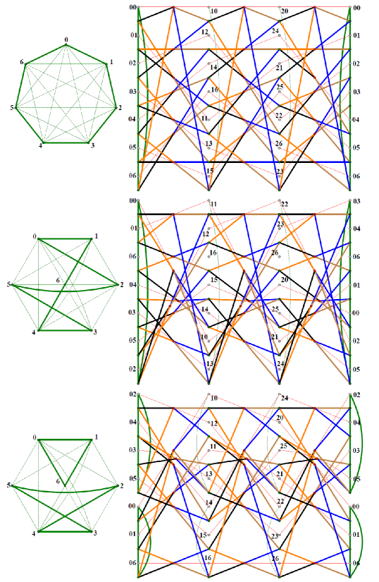
The right side of Fig. 10(a) (resp. 10(b)) represents (resp. ), where: (i) each vertex is denoted , (ii) vertices appear twice (on top and bottom, to be identified for each ), (iii) red edges are shown in thin trace, (iv) green edges arising from the cycles and of (resp. and of ) are shown in thin and dashed trace, respectively, and (v) the edges of the corresponding partial line graphs are shown in thick trace on the colors orange = , black = , hazel = and blue = , setting a tight factorization.
Vertices of green and red cycles are said to be green and red, respectively. To the left of these two graphs in Fig. 10, the corresponding green and red-green subgraphs are shown.
Note that thick edges of colors orange and black form cycles zigzagging between:
-
(A)
the vertices of each vertical green cycle (excluding the rightmost green cycle) and
-
(B)
their adjacent red vertices to their immediate right.
Also, note that thick blue and hazel edges form cycles zigzagging between:
-
(C)
the red vertices and
-
(D)
the vertices of the next vertical green cycle to their right.
The girth is realized by 4-cycles with the four colors, with a pair of edges (blue and hazel) to the left of each vertical green cycle and another pair of edges (black and orange) to the corresponding right. This is always attainable, because similar bicolored cycles can always we obtained, generating the desired tight factorizations. For instance, assigning colors to the edges , , and , respectively, yields a tight factorization of .
A code representation of the tight factorization in Fig. 10(a) is given in Table 5, where each green edge in yields a green vertex in , each red edge in yields a red vertex in , and the color of an edge between a green vertex and a red vertex is indicated between brackets: for orange, for black, for hazel and for blue.
Remark 26.
Generalizing Remark 25 to get other egc girth-tight graphs, we consider a 2-factorization of the complete graph , for odd and use it to define the barrel , with
-
(i)
as vertex set and
-
(ii)
edges forming precisely red cycles , where , and green subgraphs , where .
Fig. 11 contains representations of for three distinct 2-factorizations of , with tight factorizations represented as in Fig. 10, with green cycles so that each vertex appears just once (not twice, as in Fig. 10(a–b)). In the three cases, , and , green edges are traced thick, thin and dashed, respectively. To the left of these representations, the corresponding green subgraphs are shown. Code representations of these three tight factorizations can be found in Table 6, following the conventions of Table 5. (A different 1-factorization of that may be used with the same purpose is for example ).
In the same way, by considering the 2-factorization given in seen as the Cayley graph with formed by the 2-factors generated by the respective colors 1, 2, 3, 4, namely Hamilton cycles but , we get a tight factorization of . This is encoded in Table 7 in a similar fashion to that of Tables 4–5.
If is even, a similar generalization takes a 2-factorization of and uses the 1-factor to get a generalized mutant barrel in a likewise fashion to that of item (b) in Remark 25 but modified now via , namely with
-
(i’)
as vertex set and
-
(ii’)
edges forming precisely red cycles , where , and green subgraphs , where .
Fig. 12 represents a tight factorization of , where , represented on the upper left of the figure, is such a 2-factorization, with and as in Fig. 10, and , via corresponding thick, thin and dashed, green edge tracing. On the lower left, a representation of the red-green graph is found.
We can further extend these notions of barrel and mutant barrel by taking a cycle of copies of the 2-factors of , where but with no two contiguous and being the same element of . Here, . This defines a barrel or mutant barrel ( even in this case) and establishes the following.
Theorem 27.
The barrels and mutant barrels obtained in Remark 26 produce corresponding egc graphs and .
6 Egc girth-g-regular graphs, g larger than 4
Theorem 28.
Proof.
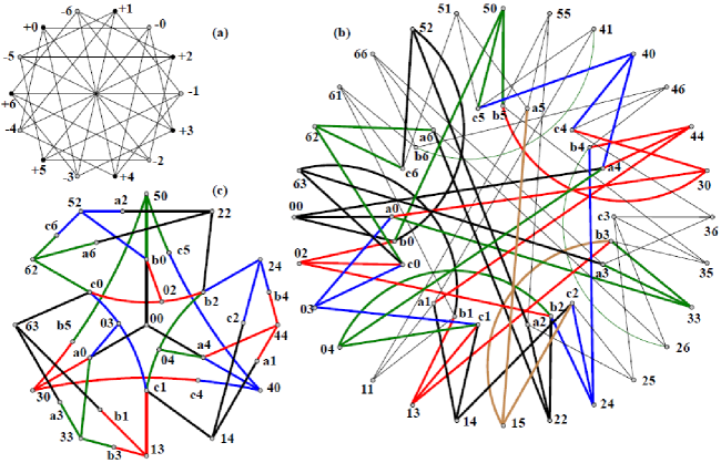
(a) The center of Fig. 13 represents colored as claimed. The vertices of are denoted (; ). An edge-color assignment for is generated mod 4 or, where is a subgroup and an ideal of , as follows:
| (19) |
where indices are taken, so colored-edge orbits are either of the form
with , and addition taken. The left of Fig. 13 contains the subgraph of spanned by the twelve 5-cycles through the black edge (where the two dashed lines must be identified), showing the disposition of twelve 5-cycles around an edge of . Moreover, the four black edges in the second line of (19) represent forty-eight tightly colored 5-cycles, (twelve passing through each black edge, corresponding to the existing color cycles
and each such cycle yields an orbit of four such 5-cycles.
Since each edge of passes through twelve 5-cycles of and , we count 5-cycles in with repetitions. Each 5-cycle in this count is repeated five times, so the number of 5-cycles in is . Thus, the number of orbits of tightly-colored 5-cycles is 48 and we obtain a tight coloring of .
(b) The upper right of Fig. 13 represents with the following 5-cycles:
The union of yields the red subgraph. Coloring tightly
with color()=color() and color()=color() makes impossible continuing coloring tightly , see as shown in the upper right of Fig. 13. Otherwise, in the lower right of Fig. 13 a forced tight coloring of , and is shown in two representations of the subgraph of induced by these 5-cycles. That leaves obstructing a tight-coloring. Thus, is not egc. ∎
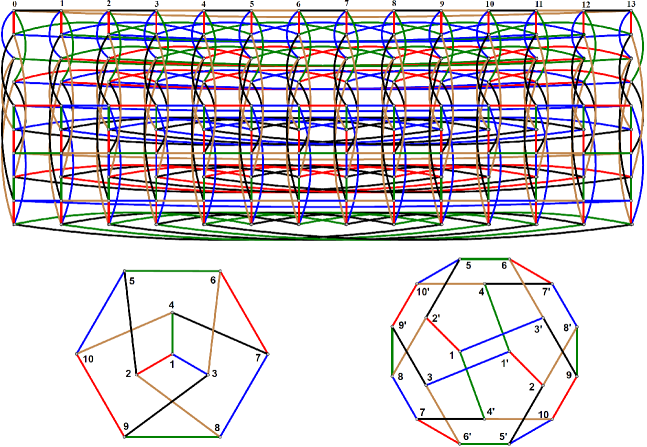
Subsequently, an egc -graph is presented by means of a construction that generalizes the barrel constructions used in Section 5, as follows. See the top of Fig. 14, where fourteen vertical copies of the Petersen graph are presented in parallel at equal distances from left to right and numbered from 0 to 13 in . The vertices of the -th copy of are denoted from top to bottom and are joined horizontally by cycles of the Cayley graph of with generator set , namely the cycles
| (23) |
Theorem 29.
There exists an egc -graph of order , for every , representing all color-cycle permutations, times each.
Proof.
We assert that an egc -graph as in the statement contains disjoint copies of . We consider the case represented in the top of Fig. 14 for and leave the details of the general case to the reader. Notice the 6-cycle in , with its three pairs of opposite vertices , , joined respectively to the neighbors of the top vertex , for . A representation of the common proper coloring of the graphs is in the lower-left part of Fig. 14, where the vertices , for and , are simply denoted . This figure shows the twelve 5-cycles of as color cycles, with red, black, blue, hazel and green taken respectively as 1, 2, 3, 4 and 5. This gives the one-to-one correspondence, call it , from the 5-cycles of onto their color 5-cycles in the top part of Table 8.
There are exactly twelve color 5-cycles; they are the targets . They are obtained from the 5!=120 permutations on five objects as the twelve orbits of the dihedral group generated both by translations and by reflections of the 5-tuples on . The edges of not in occur between different copies of ; these are colored as shown in the bottom part of Table 8. This insures the statement for , since the twelve vertical copies of are the only source of the color cycles. The extension of this for any is immediate. ∎
The dodecahedral graph with vertex set and edge set formed by an edge pair for each and an edge pair for each , is represented in the lower-right of Fig. 14, where and (that we will refer to as antipodal vertices) are respectively indicated by and , for . is a 2-covering graph of via the graph map such that .
Theorem 30.
There exists an egc -graph of order , for every .
Proof.
We consider the case and leave the details of the general case to the reader. We take seven vertical copies of presented in parallel at equal distances from left to right and numbered from 0 to 6 in . The vertices of the -th copy of are denoted and , for and are joined by the additional cycles
| (27) |
so that each such additional cycle passes through two antipodal vertices of each copy . Notice the change of the order of the indices in the assignment of the additional cycles in display (27) with respect to the one in display (23). This is done to avoid the formation of 5-cycles not entirely contained in the copies (). Since has girth 5 and signature , the graph given by the union of the seven copies and the just presented additional cycles is a -graph. By coloring the edges of the additional cycles of via the same color pattern as in Theorem 29, it is seen that is egc. ∎
The truncated-icosahedral graph is the graph of the truncated icosahedron. This is obtained from the icosahedral graph, i.e. the line graph of , by replacing each vertex of by a copy of its open neighborhood , considering all such copies pairwise disjoint, and replacing each edge of by an edge from the vertex corresponding to in to the vertex corresponding to in . Note has sixty vertices, ninety edges, twelve 5-cycles, twenty 6-cycles and signature .
Theorem 31.
There exists an egc -graph on vertices, for each integer .
Proof.
By means of a barrel-type construction as in Fig. 14, one can combine copies of and the Cayley graph of with generator set to get an egc graph as claimed. ∎
Remark 32.
The point graph of the generalized hexagon [2, p. 204], the point graph of the Van Lint–Schrijver partial geometry [2, p. 307] and the odd graph [2, p. 259] on eleven points are distance-regular with intersection arrays , and , respectively. If their chromatic number were 6, they would be -, - and -graphs, respectively, but it is known that none of them is egc.
7 Hamilton cycles and hamiltonian decomposability
Some feasible applications of egc graphs occur when the unions of pairs of composing 1-factors are Hamilton cycles, possibly attaining hamiltonian decomposability in the even-degree case. This offers a potential benefit to the applications drawn in Section 1, if an optimization/decision-making problem requires alternate inspections covering all nodes of the involved system, when the alternacy of two colors is required.
In Fig. 1, the cases (h–j) and their triangle-replaced graphs (m-o) as well as the case (u), and the 3-colored dodecahedral graph that has the case (u) as its triangle replaced graph, have the unions of any two of their 1-factors forming a Hamilton cycle, while the cases (k), (p) and (v) have those unions as disjoint pairs of two cycles of equal length. In particular, the 3-cube graph that admits just two tight factorizations, has one of them creating Hamilton cycle (case (l) via green and either red or blue edges, but not red and blue edges). The triangle-replaced graph, , has corresponding tight factorizations in cases (p–q) with similar differing properties as those of cases (k–l). Preceding Theorem 4, similar comments are made for , where is or the Coxeter graph . Recall the union of two 1-factors of is hamiltonian while the union of two 1-factors of is not.
In Fig. 2(d), the three color partitions of , namely (12)(34), (13)(24) and (14)(23), yield 2-factorizations with 2-factors formed each by two cycles of equal length . We denote this facts by writing . In a likewise fashion, we can denote toroidal items in Fig. 2 as follows: (e) , formed by 2-factorizations with 2-factors of one, three and four cycles of equal lengths 24, 6 and 8, respectively. Similarly: (f) ; (g) ; (h) ; (i) ; and (j) .
Table 9 lists various cases of Theorem 10 item 3(), indicating without parentheses or commas the triples corresponding to the numbers , and of cycles (of equal length in each case) of the respective 2-factors , and .
Remark 33.
For the toroidal cases in Theorem 10 item 3 depicted as in Fig. 2(f,g,h,j), assume that the 2-factors and complete 2-factorizations composed by 1-zigzagging cycles of equal length (i.e., composed by alternating horizontal and vertical edges) and that the 2-factors and are composed by vertical and horizontal edges, respectively. This way, while vertical edges form cycles of equal length, horizontal edges form cycles of not necessarily the same length, so the notation in the previous paragraph cannot be carried out for example for item 3() because . So we modify that notation for such cases by simply writing , that we call the star notation [9].
Theorem 34.
Proof.
We prove the statement for the toroidal cases of Theorem 10 with two colors on horizontal cycles and the other two on vertical cycles, for the factorization , and leave the rest to the reader. Consider the straight upper-right-to-lower-left line from the upper-right vertex in the cutout (Remark 5) of passing through in the lower border of and formed by the diagonals of squares representing 4-cycles of . determines two 1-zigzagging cycles through in , respectively, touching on alternate vertices of . In the end, we get parallel lines , where such that each () determines two 1-zigzagging cycles in , respectively, touching at alternate vertices of . An example is shown in Fig. 2(c) for with , where is given in black thin trace and is given in gray thin trace, (not considering here the intermittent diagonals). ∎
Corollary 35.
If , then the 2-factors , , , and are composed by a Hamilton cycle each (a total of six Hamilton cycles), comprising the 2-factorizations and .
Proof.
This is due to Remark 33 and to the quadruple equality in the statement. ∎
Additional examples are provided in display (32) for fixed , as in Theorem 10 item 3(). The reader is invited to do similarly for Theorem 10, items 3() and 3().
| (32) |
Corollary 36.
In all cases of Theorem 10 item 2(b), there are exactly two hamiltonian 2-factorizations. Moreover, the toroidal graphs in Theorem 10 are
-
1.
, for items 1(c)–2(a);
-
2.
, for item 2(b) just for ;
-
3.
, for item 2(b) just for .
Proof.
The toroidal graphs in Theorem 10 items 1() and 2() behave differently from those in Theorem 34 in that the 2-factors in question are 1-zigzagging in only one of the three 2-factorizations, while the other two 1-factorizations are 2-zigzagging, namely:
-
(a)
in Theorem 10 items 1() and 2(), just for , the 1-factorization (12)(34) is 1-zigzagging and the 1-factorizations (13)(24) and (14)(23) are 2-zigzagging;
-
(b)
in Theorem 10 item 2() just for , the 2-factorizations (12)(34)–(13)(24) are 2-zigzagging and the 2-factorization (14)(23) is 1-zigzagging.
∎
8 Applications to 3-dimensional geometry
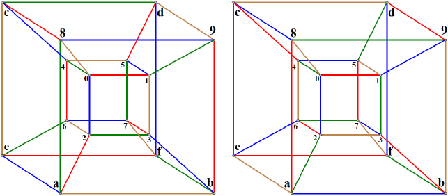
Fig. 15 redraws the two toroidal copies of in the lower center–right of Fig. 3, (which arise respectively in Subsection 3.1 from the central–right latin squares in display (6)), as edge-colored tesseracts, in order to extract piecewise linear (PL) [20] realizations of two enantiomorphic compounds of four Möbius strips each [11, 12]. In the sequel, this results to be equivalent to corresponding enantiomorphic Holden-Odom-Coxeter polylinks of four locked hollow equilateral triangles each [6, 13, 14], from a group-theoretical point of view .
8.1 Usage of the two nontrivial Latin squares in MOLS(4)
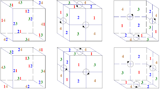
Fig. 17 contains two horizontal sets of four copies of each. A 6-cycle is distinguished in each such copy of with a respective color ( for red, for blue, for green and for hazel). Each has its with the edges marked , where for a trapezoid and for a parallelogram (quadrangles that are the faces of PL Möbius strips as in Fig. 19), for associated color and for edge direction ( for horizontal, for vertical and for in-depth). The top (resp. bottom) set has each with a one-to-one correspondence from its edges () to the edges with color and direction in the inner (outer) copy of in the left (resp. right) copy of in Fig. 15. This way, each in Fig. 17 is formed by two antipodal vertices that are joined by a color- dashed axis, allowing to visualize angle rotations representing color-and-(-or-)-preserving automorphisms that will reappear in relation to Fig. 18-19.
The two leftmost 3-cubes in Fig. 16 have each of their edges assigned a pair of colors in . The first (resp. second) color is obtained from the corresponding row of 3-cubes in Fig. 17 as the color of the only edge (resp. ) in that edge position among the four cases in the row. This allows an assignment of a color to each face quadrant of the cube, as shown on the center and right in Fig. 16, and figuring the twenty-four such quadrants in each of the two cases. Note that the faces in these cubes are given an orientation each. The color pairs in Fig. 17 can be recovered from the quadrant colors in Fig. 16 by reading them along an edge according to the corresponding face orientation.
8.2 Compound of four PL Möbius strips
Fig. 18 depicts the union of twenty-seven unit 3-cubes. In it, information carried by the top rows in Fig. 17 determines four PL trefoil knots, one per each color . These trefoil knots are indicated in thick trace along edges of the said unit cubes. These -colored thick-traced edges determine two parallel sides of either a trapezoid or a parallelogram, as illustrated in Fig. 19, for hazel color. In the case of a trapezoid (resp. parallelogram), the lengths of those sides are 3 internally and 1 externally (resp. 2 internally and 2 externally). The other two sides of each trapezoid or parallelogram are presented in thin trace in the color to distinguish them from the thick trace of the trefoil knot sides. Note that the constructed trapezoids and parallelograms determine four PL Möbius strips that give place to the following results. (Similar results for the bottom half of Fig. 17 are omitted and left for the interested reader to figure out).
Theorem 37.
There exists a maximum-area PL Möbius strip embedded in whose boundary is a PL closed curve formed by a minimum of segments parallel to the coordinate directions and whose end-vertices are points in .
Proof.
A strip as in the statement is represented in Fig. 19 (whose PL boundary is also present in Fig. 18 as the hazel trefoil knot), with the mentioned segments as in the following display (where, starting clockwise at the left upper corner of Fig. 19, colors of quadrilaterals are cited and, between parentheses, whether they are shown full or in part):
| (36) |
Here, a segment denoted stands for , with , (). In (1), each of the twelve segments are appended with its length as a subindex and an element of as a superindex, where and stand for horizontal, vertical and in-depth directions, respectively. The PL curve , a PL trefoil knot, is depicted in thick hazel trace in Fig. 18 (via unbroken unit-segment edges). ∎
Theorem 38.
The maximum number of Möbius strips in as in Theorem 37 and whose boundaries have pairwise intersections of dimension 0 (i.e., isolated points) is 4.
Proof.
To prove the statement, consider Fig. 18, where is again drawn, as well as the blue PL trefoil , defined by the segments:
| (39) |
and the green PL trefoil , defined by the segments:
| (42) |
and the brown PL trefoil , defined by the segments:
| (45) |
Observe that the six (maximum) planar faces of intersect in six pairs of segments, shown in display (36) vertically: first above and below, which form an isosceles trapezoid together with the segments and ; then, above, and below, which form a parallelogram together with the segments and , etc. Similar observations can be made with respect to displays (39)–(45). We denote such planar faces in (3-6) by , (), as on the rightmost (color 4 =) hazel 3-cube in the schematic Fig. 17.
Let us denote the maximum PL Möbius strips expanded by the PL trefoil knots , and respectively as , and . Let us look at the segmental intersections of trapezoids and parallelograms in from displays (6)–(39) above . Recall: color 1 is red, color 2 is blue, color 3 is green and color 4 is brown.
The top-front set in is trapezoid for and parallelogram for . In the upper leftmost cube in Fig. 16, let us call it , we indicate this segmental intersection by the edge-labelling pair 23, with 2 in blue and 3 in green, which are the colors used to represent and , respectively. This pair 23 labels the top-front horizontal edge in , corresponding to the position of in Fig. 18.
In all edge-labelling pairs in (Fig. 16), the first number is associated to a trapezoid and the second one to a parallelogram, each number printed in its associated color.
We subdivide the six faces of into four quarters each and label them 1 to 4, setting external counterclockwise (or internal clockwise) orientations to the faces, so that the two quarter numbers corresponding to an edge of any given face yield, via the defined orientation, the labelling pair as defined in the previous paragraph. This is represented in the center and rightmost cubes in Fig. 16.
We can identify the cube with the union of the pairwise distinct intersections , (). This way, becomes formed by the segments:
| (49) |
where each segment is suffixed with its trapezoid color number as a subindex and its parallelogram color number as a superindex. The first to third lines in (42) display those segments of parallel to the first to third coordinates, respectively. Fig. 17 represents the Möbius strips in , for , with the -colored edges corresponding to the trapezoids and parallelograms of each labeled via , ( for trapezoid; for parallelogram; for horizontal, vertical and in-depth edges of , respectively). ∎
Theorem 39.
The automorphism group of is isomorphic to . Moreover, there are only two 4-PL-Möbius-strip compounds, one of which () is the one with PL Möbius strip boundaries depicted as the PL trefoils in Fig. 18. Furthermore, these two compounds are enantiomorphic.
Proof.
By way of the reflection of about the central vertex of , each is transformed bijectively and homeomorphically into , for . The angle rotations of about the in-depth axis , the vertical axis and the horizontal axis , respectively, form the following respective transpositions on the vertices of :
| (53) |
and determine the following permutations of Möbius strips , ():
| (54) |
On the other hand, neither the reflections on the coordinate planes at nor the angle rotations preserve the union but yield a 4-PL-Möbius-strip compound that is enantiomorphic to . Moreover, is generated by , , and . ∎
8.3 Polylink of four hollow triangles
A sculpture by G. P. Odom Jr., see Fig. 20, was analyzed by H. S. M. Coxeter [6], for its geometric and symmetric properties. According to [21, p. 270], Odom and Coxeter were unaware of the earlier discovery [13] of this by A. Holden, who called it a regular polylink of four locked hollow triangles [14].
We relate the top Möbius-strip compound above to this structure, noting that the centers of the maximum linear parts of the PL trefoil knots () are the vertices of four corresponding equilateral triangles, namely (in the order of the triangle colors):
| (57) |
Each of these triangles (), gives place to a hollow triangle (i.e., a planar region bounded by two homothetic and concentric equilateral triangles [6]) by removing from the equilateral triangle whose vertices are the midpoints of the segments between the vertices of (display (57)) and . Characterized by colors, these midpoints are
| (62) |
The centers in display (57) are the vertices of an Archimedean cuboctahedron. Consider the midpoints of the sides of the triangles , namely:
| (67) |
By expressing the 3-tuples in (62) via a -matrix , we have the following correspondence from (62) to (67), in terms of the notation in Fig. 20:
| (68) |
meaning each midpoint of a between and equals a vertex of some , and vice-versa, as in Fig. 20. Take each as the 6-cycle of its vertices and side midpoints:
| (73) |
Corollary 40.
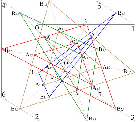
The automorphism group of the union is . In addition, , for each , is isomorphic to the dihedral group of six elements. Moreover, there are only two polylinks of four hollow triangles in , including , and these two polylinks are enantiomorphic.
Proof.
By expressing, as in Fig. 20, the vertices of by:
| (75) |
we notice that the angle rotations of around the axis line determined by the two points of color in , as indicated in Fig. 17, correspond respectively to the permutations:
| (80) |
where color 1 is red, color 2 is blue, color 3 is green and color 4 is hazel; notice also that the axes in corresponding to these colors are:
The rest of the statement arises from Theorem 39. The fact that there are two polylinks of four hollow triangles in that are enantiomorphic is inherited from Theorem 39. ∎
References
- [1] C. Armanios, A new 5–valent distance transitive graph, Ars Combin. 19A (1985), 77–85.
- [2] A. Brouwer, A, Neumaier, A. Cohen, Distance-Regular Graphs, Springer-Verlag, 1998.
- [3] C. J. Colbourn, J. H. Dinitz, Handbook of Combinatorial Designs (2nd ed.), Boca Raton: Chapman & Hall/ CRC, (2007).
- [4] J. H. Conway, N. J. A. Sloane, Sphere Packings, Lattices and Groups, (3rd ed.), Berlin, New York: Springer-Verlag, (1999).
- [5] S. L. R. Costa, R. Muniz, E. Agustini, R. Palazzo, Graphs, Tessellations and Perfect Codes in Flat Tori, IEEE Transactions on Information Theory, 50-10(2004), 2363-2377.
- [6] H. S. M. Coxeter, Symmetrical Combinations of Three or Four Hollow Triangles, The Mathematical Intelligencer, 16(3) (1994), 25–30.
- [7] H. S. M. Coxeter, Self-Dual Configurations and Regular Graphs, Bull. Amer. Math. Soc. 56 (1950), 413–455.
- [8] P. R. Cromwell, Polyhedra, Cambridge Univ. Press, Cambridge UK (1997).
- [9] I. J. Dejter, O. Serra, Efficient dominating sets in Cayley graphs, Discrete Applied Mathematics 129(2–3) (2002), 319–328.
- [10] E. Eiben, R. Jajcay, P. ’Šparl, Symmetry properties of generalized graph truncations, J. Combin. Theory, Ser. B 137 (2019) 29–131.
- [11] D. Fuchs, S. Tabachnikov, Mathematical Omnibus: Thirty Lectures on Classic Mathematics, 2007, 199–206, at http://www.math.psu.edu/tabachni/Books/taba.pdf
- [12] D. Hilbert, S. Cohn-Vossen, Geometry and the Imagination (2nd ed.), Chelsea, 1952.
- [13] A. Holden, Shapes, Spaces and Symmetry, Columbia Univ. Press, 1971.
- [14] A. Holden, Regular Polylinks, Structural Topology, 4 (1980), 41–45.
- [15] W. Imrich, S. Klavžar, D. F. Rall, Graphs and their cartesian products, A. K. Peters, (2008).
- [16] P. Potočnik, P. Spiga, G. Verret, A census of cubic vertex-transitive graphs https://staff.matapp.unimib.it/~spiga/census.html.
- [17] P. Potočnik, J. Vidali, Girth-regular graphs, Ars Mathematica Contemporanea, 17 (2019), 349–368.
- [18] P. Potočnik, S. Wilson, Tetravalent edge-transitive graphs of girth at most 4, Jour. Combin. Theory, ser. B, 97 (2007), 217–236.
- [19] P. Potočnik, S. Wilson, Linking-ring structures and tetravalent semisymmetric graphs, Ars. Math. Contemporanea, 7 (2014), 341–352.
- [20] C. P Rourke, B. J. Sanderson, Introduction to Piecewise-Linear Topology, Springer, New York, NY, 1972.
- [21] D. Schattschneider Coxeter and the Artists: 2-Way Inspiration, in The Coxeter Legacy, Reflections and Projections, (ed. C. Davis et al.), Amer. Math. Soc., 2006.
- [22] W. D. Wallis, One-Factorizations (Math. and its Appl.), Springer, NY, 1997.
- [23] S. Wilson, Uniform maps on the Klein bottle, Jour. for Geom. and Graphics, 10(2) (2006), 161–171.
- [24] S. Wilson, P. Potočnik, Recipes for edge-transitive tetravalent graphs, The Art of Discrete and Applied Mathematics, 3(1) (2020), 1–33.