PerSim: Data-efficient Offline Reinforcement
Learning with Heterogeneous Agents
via Personalized Simulators

Abstract

We consider offline reinforcement learning (RL) with heterogeneous agents under severe data scarcity, i.e., we only observe a single historical trajectory for every agent under an unknown, potentially sub-optimal policy. We find that the performance of state-of-the-art offline and model-based RL methods degrade significantly given such limited data availability, even for commonly perceived “solved” benchmark settings such as “MountainCar” and “CartPole”. To address this challenge, we propose PerSim, a model-based offline RL approach which first learns a personalized simulator for each agent by collectively using the historical trajectories across all agents, prior to learning a policy. We do so by positing that the transition dynamics across agents can be represented as a latent function of latent factors associated with agents, states, and actions; subsequently, we theoretically establish that this function is well-approximated by a “low-rank” decomposition of separable agent, state, and action latent functions. This representation suggests a simple, regularized neural network architecture to effectively learn the transition dynamics per agent, even with scarce, offline data. We perform extensive experiments across several benchmark environments and RL methods. The consistent improvement of our approach, measured in terms of both state dynamics prediction and eventual reward, confirms the efficacy of our framework in leveraging limited historical data to simultaneously learn personalized policies across agents.

1 Introduction

Reinforcement learning (RL) coupled with expressive deep neural networks has now become a generic yet powerful solution for learning complex decision-making policies for an agent of interest; it provides the key algorithmic foundation underpinning recent successes such as game solving [34, 45, 44] and robotics [30, 22]. However, many state-of-the-art RL methods are data hungry and require the ability to query samples at will, which is infeasible for numerous settings such as healthcare, autonomous driving, and socio-economic systems. As a result, there has been a rapidly growing literature on “offline RL” [31, 24, 32, 15], which focuses on leveraging existing datasets to learn decision-making policies.

Within offline RL, we consider a regime of severe data scarcity: there are multiple agents and for each agent, we only observe a single historical trajectory generated under an unknown, potentially sub-optimal policy; further, the agents are heterogeneous, i.e., each agent has unique state transition dynamics. Importantly, the characteristics of the agents that make their transition dynamics heterogeneous are latent. Using such limited offline data to simultaneously learn a good “personalized” policy for each agent is a challenging setting that has received limited attention. Below, we use a prevalent example from healthcare to motivate and argue that tackling such a challenge is an important and necessary step towards building personalized decision-making engines via RL in a variety of important applications.

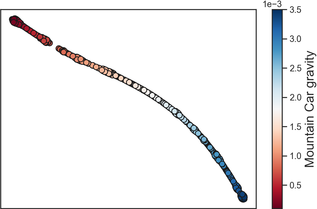
(a) MountainCar

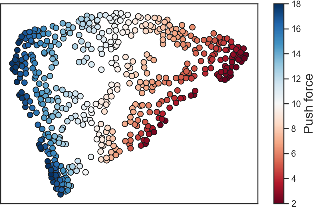
(b) CartPole

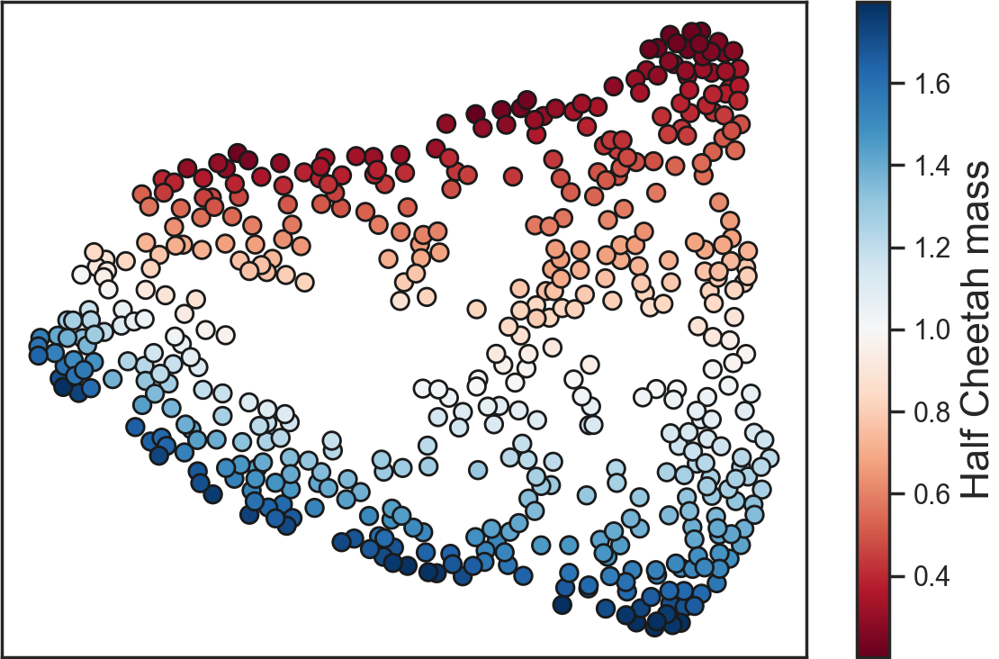
(c) HalfCheetah

Figure 1: t-SNE visualization of the learned latent factors for the 500 heterogeneous agents. Colors indicate the value of the modified parameters in each environment (e.g., gravity in MountainCar). There is an informative low-dimensional manifold induced by the agent-specific latent factors, and there is a natural direction on the manifold along which the parameters that characterize the heterogeneity vary continuously and smoothly.

A Motivating Example. Consider a pre-existing clinical dataset of patients (agents). Our goal is to design a personalized treatment plan (policy) for each patient moving forward. Notable challenges include the following: First, each patient only provides a single trajectory of their medical history. Second, each patient is heterogeneous in that they may have a varied response for a given treatment under similar medical conditions; further, the underlying reason for this heterogeneous response across patients is likely unknown and thus not recorded in the dataset. Third, in the absence of an accurate personalized “forecasting” model for a patient’s medical outcome given a treatment plan, the treatment assigned is likely to be sub-optimal. This is particularly true for complicated medical conditions like T-Cell Lymphoma. We aim to address the challenges laid out above (offline scarce data, heterogeneity, and sub-optimal policies) so as to develop a personalized “forecasting” model for each patient under any given treatment plan. Doing so will then naturally enable ideal personalized treatment policies for each patient.

Key question. Tackling a scenario like the one described above in a principled manner is the focus of this work. In particular, we seek to answer the following question:

“Can we leverage scarce, offline data collected across heterogeneous agents under unknown, sub-optimal policies to learn a personalized policy for each agent?”

Our Contributions. As our main contribution, we answer this question in the affirmative by developing a structured framework to tackle this challenging yet meaningful setting. Next, we summarize the main methodological, theoretical, algorithmic, and experimental contributions in our proposed framework.

Methodological—personalized simulators. We propose a novel methodological framework, PerSim, to learn a policy given the data availability described above. Taking inspiration from the model-based RL literature, our approach is to first build a personalized simulator for each agent. Specifically, we use the offline data collectively available across heterogeneous agents to learn the unique transition dynamics for each agent. We do this without requiring access to the covariates or features that drive the heterogeneity amongst the agents. Having constructed a personalized simulator, we then learn a personalized decision-making policy separately for each agent by simply using online model predictive control (MPC) [16, 9].

Theoretical—learning across agents. As alluded to earlier, the challenge in building a personalized simulator for each agent is that we only have access to a single offline trajectory for any given agent. Hence, each agent likely explores a very small subset of the entire state-action space. However, by viewing the trajectories across the multitude of agents collectively, we potentially have access to a relatively larger and more diverse offline dataset that covers a much richer subset of the state-action space. Still, any approach that augments the data of an agent in this manner must address the possibly large heterogeneity amongst the agents, which is challenging as we do not observe the characteristics that make agents heterogeneous. Inspired by the literature on collaborative filtering for recommendation systems, we posit that the transition dynamics across agents can be represented as a latent function of latent factors associated with agents, states, and actions. In doing so, we establish that this function is well-approximated by a “low-rank” decomposition of separable agent, state, and action latent functions (Theorem 1). Hence, for any finite sampling of the state and action spaces, accurate model learning for each agent with offline data—generated from any policy—can be reduced to estimating a low-rank tensor corresponding to agents, states, and actions. As such, low-rank tensors can provide a useful algorithmic lens to enable model learning with offline data in RL and we hope this work leads to further research studying the relationship between these seemingly disparate fields.

Algorithmic—regularizing via a latent factor model. As a consequence of our low-rank representation result, we propose a natural neural network architecture that respects the constraints induced by the factorization across agents, states, and actions (Section 4). It is this principled structure, which accounts for agent heterogeneity and regularizes the model learning, that ensures the success of our approach despite access to only scarce and heterogeneous data. Further, we propose a natural extension of our framework which generalizes to unseen agents, i.e., agents that are not observed in the offline data.

Experimental—extensive benchmarking. Using standard environments from OpenAI Gym, we extensively benchmark PerSim against four state-of-the-art methods: a model-based online RL method (CaDM) [29], two model-free offline RL method (BCQ and CQL) [15, 25], and a model-based offline RL method (MOReL) [23]. Below, we highlight six conclusions we reach from our experiments. (i) Despite access to only a single trajectory from each agent (and no access to the covariates that drive agent heterogeneity), PerSim produces accurate personalized simulators for each agent. (ii) All benchmarking algorithms perform sub-optimally for the data availability we consider, even on simple baseline environments such as MountainCar and Cartpole, which are traditionally considered to be “solved”. (iii) PerSim is able to robustly extrapolate outside the policy used to generate the offline dataset, even if the policy is highly sub-optimal (e.g., actions are sampled uniformly at random). (iv) To corroborate our latent factor representation, we find that across all environments, the learned agent-specific latent factors correspond very closely with the latent source of heterogeneity amongst agents; we re-emphasize this is despite PerSim not getting access to the agent covariates. (v) We find that augmenting the training data of an offline model-free method (e.g., BCQ) with PerSim-generated synthetic trajectories results in a significantly better average reward. (vi) As an ablation study, if we decrease the number of observed trajectories, PerSim consistently achieves a higher reward than the other baselines across most agents, indicating its robustness to data scarcity. For a visual depiction of the conclusions, see Figure 1 for the learned latent agent factors and Figure 2 for the relative prediction accuracy of the learned model using PerSim versus  [29].

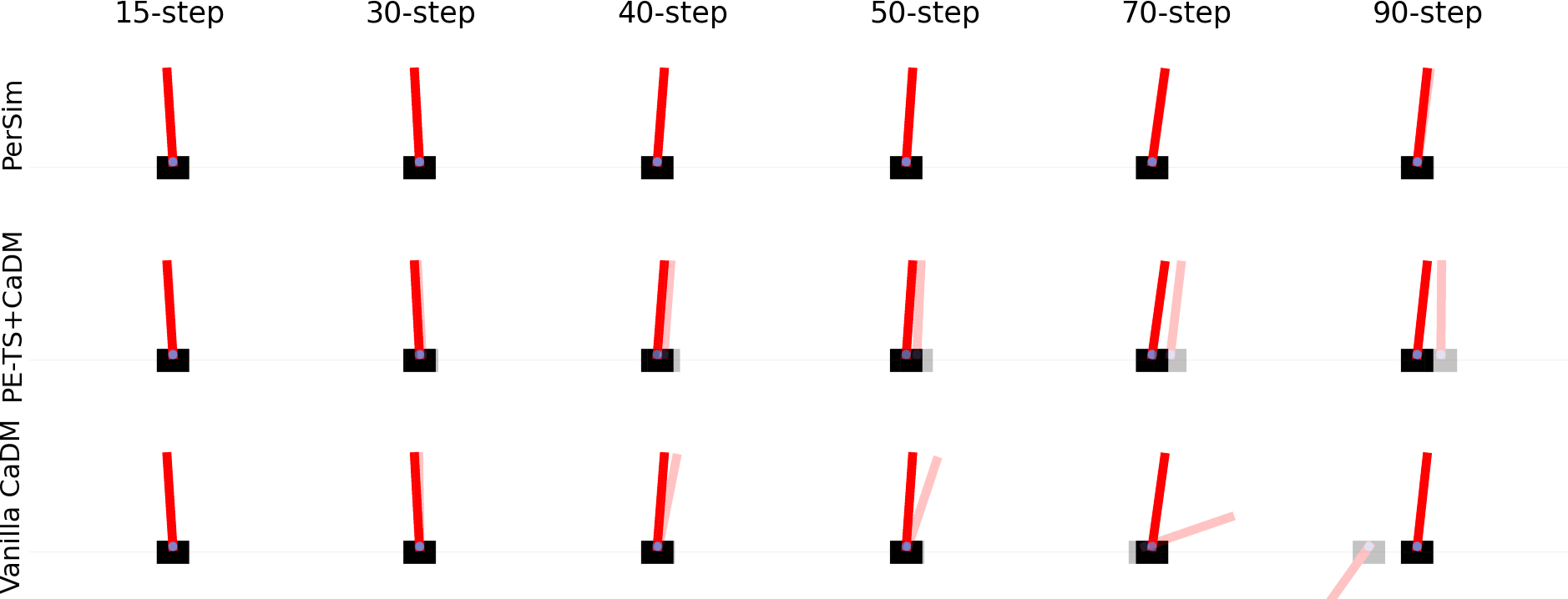
Figure 2: Visualization of prediction accuracy of the various learned models for CartPole. Actual and predicted states are denoted by the opaque and translucent objects, respectively.

Related Work. Due to space constraints, we present a short overview of the related literature. A more detailed review is provided in Appendix B.

There are two sub-fields within RL that are of particular relevance: (i) model-based online RL and (ii) model-free offline RL. (i) In the model-based RL literature, the transition dynamics (simulator) is learnt and subsequently utilized for policy learning. These methods have been found to have far better data efficiency compared to their model-free counterparts [50, 10, 11, 26, 21, 17]. However, the current model-based literature mostly focuses on the setting where one can adaptively sample trajectories in an online manner during model-learning. A few recent works [29, 36] have considered agent heterogeneity. We compare with [29] given its strong performance in handling heterogeneous agents. (ii) In the model-free offline RL literature, one uses a pre-recorded dataset to directly learn a policy, i.e., without first learning a model. Thus far, the vast majority of offline RL methods are model-free and designed for settings that allow access to numerous trajectories from a single agent, i.e., no agent heterogeneity [15, 24, 28, 32, 51, 4, 25]. To study how much offline methods suffer if agent heterogeneity is introduced, we compare with both [15] and [25] given their strong performance with offline data. We choose these baselines as they come from a well-established literature but their abilities to simultaneously handle agent heterogeneity and sparse offline data has yet to be studied.

Model-based offline RL is still a relatively nascent field. Two recent works [23, 53] have shown that, in certain settings, model-based offline methods can outperform their model-free counterparts on benchmark environments. In [53], authors exhibit this using existing online model-based methods with minimal changes. However, both works restrict attention to the setting where there is only one agent (or environment) and a large number of observations from that agent are available. Hence, we study how these methods perform when given only sparse data from heterogeneous agents, and we find their performance does suffer. Extending these model-based offline RL methods to work with sparse data from heterogeneous agents, possibly by building upon the latent low-rank functional representation we propose, remains an interesting future work.

2 Problem Statement

We consider the standard RL framework with $N$ heterogeneous agents. We index agents with $n\in[N]$. Formally, we describe our problem as a Markov Decision Process (MDP) defined by the tuple $(\mathcal{S},\mathcal{A},P_{n},R_{n},\gamma_{n},\mu_{n})$. Here, $\mathcal{S}$ and $\mathcal{A}$ denote the state and action spaces, respectively, which are common across agents. For every agent $n$, $P_{n}(s^{\prime}|s,a)$ is the unknown transition kernel, $R_{n}(s,a)$ is the immediate reward received, $\gamma_{n}\in(0,1)$ is the discounting factor, and $\mu_{n}$ is the initial state distribution.

Observations. We consider an offline RL setting where we observe a single trajectory of length $T$ for each of the $N$ heterogeneous agents. Formally, for each agent $n$ and time step $t$, let $s_{n}(t)\in\mathcal{S}$, $a_{n}(t)\in\mathcal{A}$, and $r_{n}(t)\in\mathbb{R}$ denote the observed state, action, and reward. We denote our observations as $\mathcal{D}=\{(s_{n}(t),a_{n}(t),r_{n}(t)):n\in[N],t\in[T]\}$.

Goals. We state our two primary goals below.

“Personalized” trajectory prediction. For a given agent $n$ and state-action pair $(s,a)\in\mathcal{S}\times\mathcal{A}$, we would like to estimate $\mathbb{E}[s^{\prime}_{n}|(s_{n},a_{n})=(s,a)],$ i.e., given the observations $\mathcal{D}$, we would like to build a “personalized” simulator (i.e., a model of the transition dynamic) for each agent $n$.

“Personalized” model-based policy learning. To test the efficacy of the personalized simulator, we would like to subsequently use it to learn a good decision-making policy for agent $n$, denoted as $\pi_{n}:\mathcal{S}\to\mathcal{A}$, which takes as input a given state and produces a corresponding action.

A causal inference lens. We note that this problem can be thought of as a counterfactual prediction problem. Our goal is to build a personalized simulator that answers the following question: “what would have happened had the agent took a sequence of actions other than the one we observe in the dataset?”. Broadly speaking, our aim in PerSim is to answer such questions by observing how other agents behave under varied sequences of actions. More generally, we hope PerSim serves to further link causal inference with offline RL, which is fundamentally regarded as a counterfactual inference problem  [31].

3 Latent Low-rank Factor Representation

To address the goals, we introduce a latent factor model for the transition dynamics. Leveraging latent factors have been successful in recommendation systems for overcoming heterogeneity of users. Such models have also been shown to provide a “universal” representation for multi-dimensional exchangeable arrays [5, 18]. Indeed, our latent model holds for known environments such as MountainCar.

Assume $\mathcal{S}\subseteq\mathbb{R}^{D}$, i.e., the state is $D$-dimensional. Let $s_{nd}$ refer to the $d$-th coordinate of $s_{n}$. We posit the transition dynamics (in expectation) obey the following model: for every agent $n$ and state-action pair $(s,a)$,

$$\mathbb{E}[s_{nd}^{\prime}|(s_{n},a_{n})=(s,a)]=f_{d}(\theta_{n},\rho_{s},\omega_{a}),$$ (1)

where $s_{nd}^{\prime}$ denotes the $d$-th state coordinate after taking action $a$. Here, $\theta_{n}\in\mathbb{R}^{d_{1}}$, $\rho_{s}\in\mathbb{R}^{d_{2}}$, $\omega_{a}\in\mathbb{R}^{d_{3}}$ for some $d_{1},d_{2},d_{3}\geq 1$ are latent feature vectors capturing relevant information specific to the agent, state, and action; $f_{d}:\mathbb{R}^{d_{1}}\times\mathbb{R}^{d_{2}}\times\mathbb{R}^{d_{3}}\rightarrow\mathbb{R}$ is a latent function capturing the model relationship between these latent feature vectors. We assume $f_{d}$ is $L$-Lipschitz and the latent features are bounded.

Assumption 1.

Suppose $\theta_{n}\in[0,1]^{d_{1}},\rho_{s}\in[0,1]^{d_{2}},\omega_{a}\in[0,1]^{d_{3}}$, and $f_{d}$ is $L$-Lipschitz with respect to its arguments, i.e., $|f_{d}(\theta_{n^{\prime}},\rho_{s^{\prime}},\omega_{a^{\prime}})-f_{d}(\theta_{n},\rho_{s},\omega_{a})|\leq L(\|\theta_{n^{\prime}}-\theta_{n}\|_{2}+\|\rho_{s^{\prime}}-\rho_{s}\|_{2}+\|\omega_{a^{\prime}}-\omega_{a}\|_{2}$).

For notational convenience, let $\tilde{f}_{d}:[N]\times\mathcal{S}\times\mathcal{A}\rightarrow\mathbb{R}$ be such that $\tilde{f}_{d}(n,s,a)=\mathbb{E}[s^{\prime}_{nd}|(s_{n},a_{n})=(s,a)]$.

Theorem 1.

Suppose Assumption 1 holds and without loss of generality, let $d_{1},d_{3}\leq d_{2}$. Then for all $d\in[D]$ and any $\delta>0$, there exists $h_{d}:[N]\times\mathcal{S}\times\mathcal{A}\rightarrow\mathbb{R}$, such that $h_{d}(n,s,a)=\sum^{r}_{\ell=1}u_{\ell}(n)v_{\ell}(s,d)w_{\ell}(a)$ with $r\leq C\delta^{-(d_{1}+d_{3})}$ and $\|h_{d}-\tilde{f}_{d}\|_{\infty}\leq 2L\delta$, where $C$ is an absolute constant.

Theorem 1 suggests that under the model in (1), the transition dynamics are well approximated by a low-rank order-three functional tensor representation. In fact, as we show below, for a classical non-linear dynamical system, it is exact.

An example. We show that the MountainCar transition dynamics [8] exactly satisfies this low-rank tensor representation. In MountainCar, the state $s_{n}=[s_{n1},s_{n2}]$ consists of car (agent) $n$’s position and velocity, i.e., $\mathcal{S}\subseteq\mathbb{R}^{2}$; the action $a_{n}$ is a scalar that represents the applied acceleration, i.e., $\mathcal{A}\subseteq\mathbb{R}$. For car $n$, parameterized by gravity $g_{n}$, the (deterministic) transition dynamics given action $a_{n}$ are

$$s^{\prime}_{n1}=\ s_{n1}+s_{n2}-\frac{g_{n}\cos(3s_{n1})}{2}+\frac{a_{n}}{2},\quad s^{\prime}_{n2}=s_{n2}-g_{n}\cos(3s_{n1})+a_{n}.$$

Proposition 1.

In MountainCar, $r=3$.

Model Learning & Tensor Estimation. Consider any finite sampling of the states $\tilde{\mathcal{S}}\subset\mathcal{S}$ and actions $\tilde{\mathcal{A}}\subset\mathcal{A}$. Let $\mathcal{X}=[X_{nsad}]\in\mathbb{R}^{N\times|\tilde{\mathcal{S}}|\times|\tilde{\mathcal{A}}|\times D}$ be the order-four tensor, where $X_{nsad}=f_{d}(\theta_{n},\rho_{s},\omega_{a})$. Hence, to learn the model of transition dynamics for all the agents over $\tilde{\mathcal{S}}$, $\tilde{\mathcal{A}}$, it is sufficient to estimate the tensor, $\mathcal{X}$, from observed data. The offline data collected for a given policy induces a corresponding observation pattern of this tensor. Whether the complete tensor is recoverable, is determined by this induced sparsity pattern and the rank of $\mathcal{X}$. Notably, Theorem 1 suggests that $\mathcal{X}$ is low-rank under mild regularity conditions. Therefore, the question of model identification, i.e., completing the tensor $\mathcal{X}$, boils down to conditions on the offline data in terms of the observation pattern that it induces in the tensor. In the existing tensor estimation literature, there are few sparsity patterns for which the underlying tensor can be provably recovered, provided $\mathcal{X}$ has a low-rank structure. They include: (i) each entry of the tensor is observed independently at random with sufficiently high-probability [6, 35, 43]; (ii) the entries that are observed are block-structured [2, 42]. However, the most general set of conditions on the sparsity pattern under which the underlying tensor can be faithfully estimated, i.e., the model is identified for our setup, remains an important and active area of research.

4 PerSim Algorithm

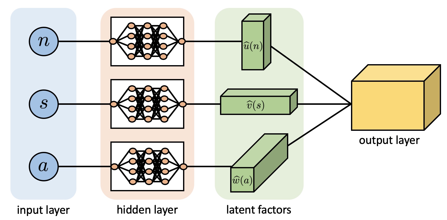
Figure 3: Neural Network Architecture

We now detail our proposed algorithm which is composed of two steps: (i) build a personalized simulator for each agent $n$ given offline observations $\mathcal{D}$, which is comprised of a single trajectory per agent; (ii) learn a personalized decision-making policy using MPC.

Step 1. Learning Personalized Simulators. Theorem 1 suggests that the transition dynamics can be represented as a low-rank tensor function with latent functions associated with the agents, states, and actions. This guides the design of a simple, regularized neural network architecture: we use three separate neural networks to learn the agent, state, and action latent functions, i.e., we remove any edges between these three neural networks. See Figure 1 for a visual depiction of our proposed architecture. Specifically, to estimate the next state for a given agent $n$ and state-action pair $(s,a)\in\mathcal{S}\times\mathcal{A}$, we learn the following functions:

1. An agent encoder $g_{u}:[N]\to\mathbb{R}^{r}$, parameterized by $\psi$, which estimates the latent function associated with an agent, i.e., $\widehat{u}(n)=g_{u}(n;\psi)$.

2. A state encoder $g_{v}:\mathcal{S}\rightarrow\mathbb{R}^{D\times r}$ parameterized by $\phi$, which estimates $D$ latent functions, where each vector is associated with the corresponding state coordinate, i.e., $\widehat{v}(s):=(\widehat{v}(s,1),\ \dots,\ \widehat{v}(s,D))^{T}=g_{v}(s;\phi).$

3. An action encoder $g_{w}:\mathcal{A}\rightarrow\mathbb{R}^{r}$ parameterized by $\theta$, which estimates the latent function associated with the action, i.e., $\widehat{w}(a)=g_{w}(a;\theta)$.

Then, our estimate of the expected $d$-th coordinate of the next state is given by $\widehat{\mathbb{E}}[s_{nd}^{\prime}|(s_{n},a_{n})=(s,a)]=\sum_{\ell=1}^{r}\widehat{u}_{\ell}(n)\widehat{v}_{\ell}(s,d)\widehat{w}_{\ell}(a).$ We optimize our agent, state, and action encoders by minimizing the squared loss: $\mathcal{L}(s,a,n,s^{\prime};\psi,\phi,\theta)=\sum_{d=1}^{D}\Big{(}s_{nd}^{\prime}-\sum_{\ell=1}^{r}\widehat{u}_{\ell}(n)\widehat{v}_{\ell}(s,d)\widehat{w}_{\ell}(a)\Big{)}^{2}.$

Step 2. Learning a Decision-making Policy. We use MPC to select the next action, as common practice in the literature [29]. Since the offline data may not span the entire state-action space, planning using a learned simulator without any regularization may result in “model exploitation” [31]. Thus, when choosing the action via MPC, we choose the first action from the sequence of actions with the best average reward across an ensemble of $M$ simulators. In our experiments, we find that the simple technique of using the state difference instead of the raw state improves performance. For a detailed description of the algorithm, including the pseudo-code, please refer to Appendix D.

5 Experiments

In this section, through a systematic collection of experiments on a variety of benchmark environments, we demonstrate that PerSim consistently outperforms state-of-the-art model-based and offline model-free RL algorithms, in terms of prediction error and reward, for the data regime we consider.

5.1 Setup and Benchmarks

We evaluate PerSim on three benchmark environments from OpenAI Gym [8]: MountainCar, CartPole, and HalfCheetah. A detailed description of each environment can be found in Appendix E.

Heterogeneous Agents. We introduce agent heterogeneity across the various environments by modifying the covariates that characterize the transition dynamics of an agent. This is in line with what has been done in the literature [29] to study algorithmic robustness to agent heterogeneity. The range of parameters we consider for each of the three environments is given in Table 4 of Appendix E; for example, we create heterogeneous agents in MountainCar by varying the gravity parameter of a car (agent) within the interval $[0.01,0.035]$.

For each environment, we uniformly sample 500 covariates (i.e., heterogeneous agents) from the parameter ranges displayed in Table 4 of Appendix E. We then select five of the 500 agents to be our “test” agents, i.e., these are the agents for which we report the prediction error and eventual reward for the various RL algorithms. Our rationale for selecting these five agents is as follows: one of the five is the default covariate parameter in an environment; the other four are selected so as to cover the “extremes” of the parameter range. Due to space constraints, we show results for three test agents in this section; the results for the remaining two agents can be found in Appendix F. We note that the conclusions we draw from our experiments continue to hold over all test agents we evaluate on.

Offline Data from Sub-optimal Policies. To study how robust the various RL algorithms are to the “optimality” of the sampling policy used to generate the historical trajectories, we create four offline datasets of 500 trajectories (one per agent) for each environment as follows:

(i) Pure policy. For each agent, actions are sampled according to a fixed policy that has been trained to achieve “good” performance. Specifically, for each environment, we first train a policy in an online fashion for a few training agents (see Table 4 for details). We pick the training agents to be uniformly spread throughout the training range to ensure reasonable performance for all agents. See Appendix E for details about the average reward achieved across all agents using this procedure. For MountainCar and CartPole, we use DQN [34] to train the sampling policy; for HalfCheetah, we use TD3 [14]. The policies are trained to achieve rewards of approximately -200, 120, and 3000 for MountainCar, CartPole, and HalfCheetah, respectively. Then for each of the 500 agents, we sample one trajectory using the policy trained on the training agent with the closest parameter value. (ii) Random. Actions are selected uniformly at random. (iii/iv) Pure-$\varepsilon$-20/Pure-$\varepsilon$-40. For Pure-$\varepsilon$-20/40, actions are selected uniformly at random with probability 0.2/0.4, respectively, and selected via the pure policy otherwise.

The “pure policy” dataset has relatively optimal transition dynamics for each agent compared to the other three policies. This is likely the ideal scenario when we only have access to limited offline data. However, such an ideal sampling procedure is hardly met in practice. Real-world data often contains at least some amount of “trial and error” in terms of how actions are chosen; we model this by sampling a fraction of the trajectory at random.

Benchmarking Algorithms. We compare with four state-of-the-art RL algorithms; (i) one from the online model-based literature; (ii) two from the offline model-free literature; (iii) and one offline model-based approach. In Appendix D, we give implementation details.

Vanilla CaDM + PE-TS CaDM [29]. As aforementioned, we choose CaDM as a baseline given its superior performance against other popular model-based (and meta-learning) methods in handling heterogeneous agents. CaDM tackles heterogeneity by learning a context vector using the recent trajectory of a given agent, with a common context encoder across all agents. In our evaluation, we compare against two CaDM variants discussed in [29] with respect to both model prediction error and eventual reward.

BCQ-P + BCQ-A [15]. BCQ is an offline model-free RL method that has been shown to exhibit excellent performance in the standard offline setting. In light of this, we consider two BCQ baselines: (i) BCQ-Population (or BCQ-P), where a single policy is trained using data from all available (heterogeneous) agents, i.e., all 500 observed trajectories; (ii) BCQ-Agent (or BCQ-A), where a separate policy is learned for each of the test agents using just the single observed trajectory associated with that test agent. We compare PerSim against both BCQ variants with respect to the eventual reward in order to study the effect that data scarcity and agent heterogeneity can have on standard offline RL methods.

CQL-P + CQL-A [25]. CQL is considered one of the state-of-the-art offline model-free RL methods. Similar to BCQ, we consider two CQL baselines: CQL-P and CQL-A, which are defined analogously to BCQ-P and BCQ-A.

MOReL-P + MOReL-A [23]. MOReL is a recent work that proposes a model-based approach for offline RL. MOReL does not consider a setting where data is collected from heterogeneous agents, unlike CaDM and PerSim. However, we include MOReL as a baseline to provide a more comprehensive evaluation. Similar to BCQ and CQL, we consider two MOReL baselines: MOReL-P and MOReL-A, which are defined analogously to BCQ-P and BCQ-A.

5.2 Model Learning: Prediction Error

The core of PerSim is to build a personalized simulator for each agent. This is also the case for two of the methods we compare against, Vanilla CaDM and PE-TS CaDM. Thus, for each of these algorithms, we first evaluate the accuracy of the learned transition dynamics for each agent, focusing on long-horizon model prediction. Specifically, given an initial state and an unseen sequence of 50 actions, the task is to predict the next 50-step state trajectory for the test agents. The sequence of 50 actions are chosen according to an unseen test policy that is different than the policies used to sample the training dataset. Precisely , the test policies are fitted via DQN for MountainCar and CartPole and via TD3 for HalfCheetah for the agent with the default covariate parameters. The test policies were such that they achieved rewards of -150, 150, and 4000 for MountainCar, CartPole and HalfCheetah, respectively.

For each environment and for PerSim, Vanilla CaDM, and PE-TS CaDM, we train four separate models using each of the four offline datasets described earlier. We repeat the process 200 times (totaling 200 trajectories for each test agent) and report the mean root-mean-squared error (RMSE) over all 50-steps and over all 200 trajectories. In addition to RMSE, we provide the median $R^{2}$ (in parentheses within the tables) to facilitate a better comparison in terms of relative error. The results are summarized in Table 1 for MountainCar, CartPole, and HalfCheetah. Further experimental results regarding prediction error can be found in Appendix F.1.

Table 1: Prediction error.

		MountainCar			CartPole			HalfCheetah
Data	Method	0.01	0.025	0.035	(2/0.5)	(10/0.85)	(10/0.15)	(0.3/1.7)	(1.7/0.3)	(0.3/0.3)
Pure	PerSim	0.025 (0.97)	0.014 (0.94)	0.039 (0.80)	0.01 (1.00)	0.01 (1.00)	0.035 (1.00)	1.194 (0.92)	4.064 (0.67)	4.070 (0.81)
	Vanilla CaDM	0.149 (0.74)	0.177 (-18.4)	0.238 (-30.1)	0.403 (0.71)	0.039 (0.98)	2.531 (-0.53)	3.902 (0.47)	3.851(0.49)	6.308 (0.38)
	PE-TS CaDM	0.326 (-1.91)	0.154 (-1.11)	0.148 (-0.18)	0.031 (0.99)	0.06 (1.00)	0.319 (0.65)	3.147 (0.61)	3.080 (0.68)	5.270 (0.57)
Random	PerSim	0.04 (1.00)	0.01 (1.00)	0.01 (1.00)	0.014 (0.98)	0.06 (1.00)	0.152 (0.88)	1.194 (0.92)	4.064 (0.67)	4.070 (0.81)
	Vanilla CaDM	0.256 (0.43)	0.134 (0.71)	0.217 (-1.77)	0.172 (0.10)	0.098 (0.64)	3.307 (-0.73)	4.030 (0.44)	4.121 (0.43)	4.446 (0.67)
	PE-TS CaDM	0.242 (0.31)	0.101 (0.87)	0.075 (0.97)	0.564 (-1.36)	0.216 (0.45)	3.764 (-1.10)	2.735 (0.73)	2.756 (0.69)	4.141 (0.77)
Pure-$\varepsilon$-20	PerSim	0.04 (1.00)	0.02 (1.00)	0.04 (1.00)	0.0 (1.00)	0.01 (1.00)	0.048 (0.98)	1.172 (0.92)	4.283 (0.66)	3.832 (0.84)
	Vanilla CaDM	0.227 (0.31)	0.101 (-0.37)	0.157 (-2.25)	0.270 (-0.98)	0.058 (0.94)	2.193 (-0.43)	3.613 (0.53)	3.455 (0.54)	6.046 (0.48)
	PE-TS CaDM	0.350 (-2.57)	0.139 (0.75)	0.130 (0.89)	0.639 (-1.21)	0.148 (0.38)	2.680 (-0.56)	2.913 (0.70)	2.959 (0.65)	4.818 (0.65)
Pure-$\varepsilon$-40	PerSim	0.06 (1.00)	0.06 (0.99)	0.03 (1.00)	0.0 (1.00)	0.0 (1.00)	0.018 (1.00)	1.016 (0.94)	4.021 (0.66)	3.742 (0.85)
	Vanilla CaDM	0.199 (0.54)	0.119 (0.38)	0.187 (-9.00)	0.233 (-0.88)	0.035 (0.99)	3.286 (-0.62)	3.685 (0.49)	3.612 (0.48)	6.000 (0.39)
	PE-TS CaDM	0.639 (-2.27)	0.192 (-6.06)	0.157 (0.55)	0.051 (0.98)	0.010 (1.00)	0.411 (0.55)	3.021 (0.67)	3.025 (0.61)	5.075 (0.62)

PerSim Accurately Learns Personalized Simulators. Consistently across environments, PerSim outperforms both Vanilla CaDM and PE-TS CaDM for most test agents. RMSE for PerSim is notably lower by orders of magnitude in MountainCar and CartPole. Indeed, in these two environments, $R^{2}$ for PerSim is nearly one (i.e., the maximum achievable) across most agents, while for the two CaDM variants it is notably lower. In a number of experiments, the two CaDM variants have negative $R^{2}$ values, i.e., their predictions are worse than simply predicting the average true state across the test trajectory. For HalfCheetah, which has a relatively high-dimensional state space (it is 18-dimensional), PerSim continues to deliver reasonably good predictions for each agent despite the challenging data availability. Though PerSim still outperforms CaDM in HalfCheetah, we note CaDM’s performance is more comparable in this environment.

For a more visual representation of PerSim’s prediction accuracy, refer back to Figure 2 in Section 1, which shows the predicted and actual state for different horizon lengths in CartPole; there, we see that PerSim consistently produces state predictions that closely match the actual state observed from the true environment. Additional visualizations across environments are provided in Appendix F.1

Rethinking Model-based RL for Our Setting. Altogether, these results indicate that existing model-based RL methods cannot effectively learn a model of the transition dynamics simultaneously across all heterogeneous agents (e.g., CaDM sometimes has negative $R^{2}$ values) if only given access to sparse offline data. It has been exhibited [19, 53, 31] that certain model-based methods that were originally targeted for the online setting can potentially still deliver reasonable performance with offline data and minimal algorithmic change. Our experiments offer evidence that model-based RL methods, even those which are optimized to work with heterogeneous agents, do not provide a uniformly good “plug-in” solution for the particular data availability we consider. In contrast, our latent factor approach consistently learns a reasonably good model of the dynamics across all agents.

Latent Factors Capture Agent Heterogeneity. The poor performance of standard model-based RL methods for the data availability setting we consider emphasizes the need for new principled approaches. Ours is one such approach, where we posit a low-rank latent factor representation of the agents, states, and actions. To further validate our approach, we visualize the learned latent agent factors associated with the 500 heterogeneous agents in each environment in Figure 1 of Section 1. Pleasingly, across environments, the latent factors correspond closely with the heterogeneity across agents.

5.3 Policy Performance: Average Reward

In this section, we evaluate the average reward achieved by PerSim compared to several state-of-the-art model-based and model-free offline RL methods. For the PerSim and the two CaDM variants, we follow [29] in utilizing MPC to make policy decisions on top of the learned model. We include an additional baseline, “True env + MPC”, where we apply MPC on top of the actual ground-truth environment; this allows us to quantify the difference in reward when using MPC with the actual environment versus the learned simulators. For the model-free methods (e.g., BCQ and CQL variants), we can directly apply the policy resulted from the learned $Q$-value. Likewise, we directly apply the policy trained by MOReL. We use the trained policy for this model-based method instead of utilizing MPC to faithfully follow the method described in [23].

We evaluate the performance of each method using the average reward over 20 episodes for model-based methods and the average over 100 episodes for model-free methods. We repeat each experiment five times and report the mean and standard deviation. Table 2 presents the results for MountainCar, CartPole, and HalfCheetah. Further experimental results regarding reward are given in Appendix F.2.

Table 2: Average reward.

		MountainCar			CartPole			HalfCheetah
Data	Method	0.01	0.025	0.035	(2/0.5)	(10/0.85)	(10/0.15)	(0.3/1.7)	(1.7/0.3)	(0.3/0.3)
Pure	PerSim	-56.80$\pm$1.83	-189.4$\pm$6.44	-210.6$\pm$4.27	199.7$\pm$0.58	193.8$\pm$4.28	192.0$\pm$2.28	1984 $\pm$763	997.0$\pm$403	714.7$\pm$314
	Vanilla CaDM	-106.3$\pm$44.1	-432.3$\pm$117	-471.8$\pm$43.0	168.0$\pm$19.7	190.8$\pm$6.80	58.10$\pm$10.7	50.31$\pm$71.7	-134.0$\pm$81.1	11.39$\pm$171
	PE-TS CaDM	-74.23$\pm$16.5	-492.3$\pm$13.3	-500.0$\pm$0.0	92.30$\pm$44.8	193.6$\pm$8.30	127.5$\pm$9.50	481.1$\pm$252	503.7$\pm$181	553.0$\pm$127
	BCQ-P	-67.60$\pm$22.3	-267.8$\pm$202	-295.1$\pm$180	166.2$\pm$39.3	181.2$\pm$13.5	182.8$\pm$15.0	549.8$\pm$322	2006 $\pm$153	-65.18$\pm$92.8
	BCQ-A	-44.79$\pm$0.08	-380.7$\pm$170	-500.0$\pm$0.0	65.40$\pm$67.5	79.20$\pm$69.5	132.1$\pm$85.0	-262.7$\pm$96.6	-139.0$\pm$236	165.6$\pm$83.1
	CQL-P	-176.1$\pm$45.2	-316.4$\pm$26.4	-362.9$\pm$17.9	154.4$\pm$17.7	190.9$\pm$0.7	170.2$\pm$0.6	-353.5$\pm$78.4	-453.6$\pm$71.9	-476.7$\pm$129
	CQL-A	-44.60$\pm$0.0	-500.0$\pm$0.0	-499.3$\pm$0.7	122.8$\pm$63.4	179.4$\pm$20.6	193.6$\pm$5.4	-65.00$\pm$105	-257.9$\pm$35.9	-279.6$\pm$34.4
	MOReL-P	-46.00$\pm$1.1	-500.0$\pm$0.0	-500.0$\pm$0.0	35.80$\pm$1.4	96.60$\pm$24.1	66.40$\pm$24.5	-1297 $\pm$519	-1256 $\pm$627	-1470 $\pm$727
	MOReL-A	-373.0$\pm$33.5	-500.0$\pm$0.0	-500.0$\pm$0.0	33.70$\pm$3.8	27.50$\pm$0.1	10.10$\pm$0.7	-726.2$\pm$4.9	-666.1$\pm$42.6	-841.7$\pm$39.5
Random	PerSim	-57.70$\pm$5.63	-186.6$\pm$4.25	-210.1$\pm$4.48	197.7$\pm$7.82	193.0$\pm$6.60	185.7$\pm$ 3.49	2124 $\pm$518	2060 $\pm$900	472.0$\pm$56.9
	Vanilla CaDM	-62.57$\pm$5.11	-479.3$\pm$21.7	-497.5$\pm$4.39	150.5$\pm$15.7	175.6$\pm$5.80	65.10$\pm$16.3	288.4$\pm$32.4	362.9$\pm$55.4	351.8$\pm$34.9
	PE-TS CaDM	-82.00$\pm$3.47	-500.0$\pm$0.0	-500.0$\pm$0.0	88.60$\pm$18.5	196.1$\pm$3.00	171.0$\pm$21.7	754.6$\pm$242	744.5$\pm$281	767.4$\pm$214
	BCQ-P	-500.0$\pm$0.0	-500.0$\pm$0.0	-500.0$\pm$0.0	44.80$\pm$34.0	57.91$\pm$53.0	36.40$\pm$36.0	-1.460$\pm$0.16	-1.750$\pm$0.22	-1.690$\pm$0.19
	BCQ-A	-500.0$\pm$0.0	-500.0$\pm$0.0	-500.0$\pm$0.0	43.90$\pm$16.4	21.10$\pm$5.81	39.50$\pm$12.1	-498.9$\pm$108	-113.3$\pm$13.0	-159.5$\pm$51.7
	CQL-P	-500.0$\pm$0.0	-500.0$\pm$0.0	-500.0$\pm$0.0	39.90$\pm$29.9	77.90$\pm$26.2	148.7$\pm$17.1	-481.5$\pm$25.9	-442.2$\pm$56.4	-672.4$\pm$17.6
	CQL-A	-500.0$\pm$0.0	-500.0$\pm$0.0	-500.0$\pm$0.0	67.40$\pm$49.1	30.60$\pm$26.4	7.000$\pm$1.9	-0.700$\pm$0.4	-2.800$\pm$0.8	-0.600$\pm$0.3
	MOReL-P	-45.00$\pm$0.3	-500.0$\pm$0.0	-500.0$\pm$0.0	50.20$\pm$7.9	68.90$\pm$17.4	40.40$\pm$12.4	-102.3$\pm$45.7	-188.7$\pm$37.1	-181.0$\pm$67.7
	MOReL-A	-495.0$\pm$3.9	-500.0$\pm$0.0	-500.0$\pm$0.0	35.80$\pm$0.4	27.50$\pm$0.7	10.60$\pm$0.2	-430.8$\pm$195	-673.7$\pm$39.3	-365.5$\pm$97.4
Pure-$\varepsilon$-20	PerSim	-54.20$\pm$0.56	-191.2$\pm$6.70	-199.7$\pm$3.99	199.8$\pm$0.24	199.1$\pm$1.30	197.8$\pm$1.68	3186 $\pm$604	1032$\pm$232	1121$\pm$243
	Vanilla CaDM	-56.73$\pm$4.20	-463.2$\pm$57.5	-478.9$\pm$35.8	171.1$\pm$38.1	193.4$\pm$2.10	64.20$\pm$10.0	412.0$\pm$152	31.92$\pm$109	460.2$\pm$159
	PE-TS CaDM	-107.6$\pm$36.3	-500.0$\pm$0.0	-500.0$\pm$0.0	98.30$\pm$42.9	198.6$\pm$0.40	141.1$\pm$12.0	1082 $\pm$126	1125 $\pm$132	1067 $\pm$64.3
	BCQ-P	-71.21$\pm$24.4	-286.6$\pm$196	-328.3$\pm$158	98.90$\pm$30.2	162.1$\pm$15.5	86.10$\pm$72.1	254.6$\pm$352	406.7$\pm$71.1	385.9$\pm$57.1
	BCQ-A	-364.5$\pm$180	-260.6$\pm$51.4	-204.5$\pm$68.9	67.30$\pm$62.2	65.60$\pm$51.8	140.0$\pm$80.6	376.8$\pm$102	84.66$\pm$53.3	230.1$\pm$10.0
	CQL-P	-79.40$\pm$16.1	-357.9$\pm$12.5	-407.6$\pm$15.3	163.7$\pm$13.6	198.1$\pm$2.6	190.4$\pm$6.6	838.7$\pm$24.5	3155 $\pm$125	539.9$\pm$313
	CQL-A	-44.70$\pm$0.1	-500.0$\pm$0.0	-500.0$\pm$0.0	42.40$\pm$11.9	199.0$\pm$1.9	199.8$\pm$0.2	-15.50$\pm$9.0	-73.00$\pm$26.3	-108.0$\pm$64.6
	MOReL-P	-83.50$\pm$15.6	-357.0$\pm$13.8	-407.4$\pm$17.1	166.7$\pm$13.6	197.7$\pm$2.7	189.4$\pm$7.1	0.600$\pm$209	-171.2$\pm$125	-219.9$\pm$76.7
	MOReL-A	-44.60$\pm$0.1	-500.0$\pm$0.0	-500.0$\pm$0.0	41.40$\pm$13.1	198.8$\pm$2.1	199.9$\pm$0.2	-781.0$\pm$37.9	-613.1$\pm$49.9	-847.1$\pm$64.7
Pure-$\varepsilon$-40	PerSim	-54.60$\pm$0.55	-189.7$\pm$7.14	-200.3$\pm$2.26	199.9$\pm$0.18	198.0$\pm$1.21	197.4$\pm$1.72	2590 $\pm$813	1016 $\pm$283	1365 $\pm$582
	Vanilla CaDM	-55.23$\pm$0.76	-481.7$\pm$25.3	-496.2$\pm$4.31	160.6$\pm$46.6	191.9$\pm$6.40	79.60$\pm$31.6	465.6$\pm$49.2	452.7$\pm$130	720.0$\pm$74.9
	PE-TS CaDM	-102.3$\pm$20.3	-500.0$\pm$0.0	-500.0$\pm$0.0	91.90$\pm$67.6	197.0$\pm$1.40	143.5$\pm$17.5	1500 $\pm$246	1218 $\pm$221	1339 $\pm$54.8
	BCQ-P	-50.01$\pm$7.50	-373.6$\pm$180	-352.0$\pm$211	28.90$\pm$6.80	31.80$\pm$25.9	18.50$\pm$11.1	78.25$\pm$200	173.8$\pm$189	417.1$\pm$155
	BCQ-A	-94.87$\pm$0.88	-358.7$\pm$201	-486.5$\pm$20.6	34.60$\pm$1.55	47.71$\pm$48.7	23.20$\pm$9.44	269.2$\pm$60.7	-181.5$\pm$57.4	193.0$\pm$31.8
	CQL-P	-61.40$\pm$2.1	-366.9$\pm$21.3	-429.1$\pm$18.8	182.2$\pm$18.0	198.3$\pm$2.9	191.9$\pm$8.7	808.5$\pm$240	1662 $\pm$221	-156.3$\pm$119
	CQL-A	-44.70$\pm$0.0	-500.0$\pm$0.0	-490.1$\pm$9.6	20.70$\pm$0.7	134.2$\pm$10.2	9.700$\pm$8.1	-6.200$\pm$2.9	-386.0$\pm$42.4	37.10$\pm$154
	MOReL-P	-61.30$\pm$2.3	-373.2$\pm$19.3	-428.5$\pm$21.0	178.9$\pm$18.7	197.9$\pm$3.1	190.6$\pm$9.3	8.500$\pm$61.6	-114.2$\pm$72.2	-195.9$\pm$77.3
	MOReL-A	-44.70$\pm$0.0	-500.0$\pm$0.0	-492.1$\pm$9.3	20.70$\pm$0.8	135.4$\pm$11.2	10.80$\pm$8.8	-325.9$\pm$17.1	-644.5$\pm$18.8	-798.8$\pm$130
	True env+MPC	-53.95$\pm$4.10	-182.9$\pm$22.9	-197.5$\pm$20.7	200.0$\pm$0.0	198.4$\pm$7.20	200.0$\pm$0.0	7459 $\pm$171	42893$\pm$6959	66675$\pm$9364

As a high-level summary, in most experiments, PerSim either achieves the best reward or close to it. This not only reaffirms our prediction results in Section 5.2, but also is particularly encouraging for PerSim since the policy utilized is simply MPC and not optimized as done in model-free approaches and in MOReL. Furthermore, these results corroborate the appropriateness of our low-rank latent factor representation and our overall methodological framework as a principled solution to this challenging yet meaningful setting within offline RL. In what follows, we highlight additional interesting conclusions.

“Solved” Environments are Not Actually Solved. MountainCar and CartPole are commonly perceived as simple, “solved” environments within the RL literature. Yet, results in Table 2 demonstrate that the offline setting with scarce and heterogeneous data impose unique challenges, and undoubtedly warrants a new methodology. We find state-of-the-art model-based and model-free methods perform poorly on some of the test agents in MountainCar and CartPole. In comparison, PerSim’s performance in these environments is close to that of MPC planning using the ground-truth environment across all test agents, thereby confirming the success of learning the personalized simulators in Step 1 of our algorithm. In certain rare cases (e.g., MountainCar test agent 0.01) where other baselines have a comparable performance to PerSim, we see that these baselines even outperforms True env + MPC. This indicates that the bottleneck in these experiments is using MPC for policy planning rather than the learned simulator in PerSim.

PerSim Robustly Extrapolates with Sub-optimal Data. Crucially, across all environments and offline data generating processes, PerSim remains the most consistent and robust winner. This is a much desired property for offline RL. In real-world applications, the policy used to generate the offline dataset is likely unknown. Thus, for broad applicability of a RL methodological framework, it is vital that it is robust to sub-optimality in how the dataset was generated, e.g., the dataset may contain a significant amount of “trial and error” (i.e, randomized actions). Indeed, this is one of the primary motivations to use RL in such settings in the first place.

As mentioned earlier, the four offline datasets correspond to varying degrees of “optimality” of the policy used to sample agent trajectories. We highlight that PerSim achieves uniformly good reward, even with random data, i.e., the offline trajectories are produced using totally random actions. This showcases that by first learning a personalized simulator for each agent, PerSim is able to robustly extrapolate outside the policy used to generate the data, however sub-optimal that policy might be. In contrast, BCQ and CQL are not robust to such sub-optimality in the offline data generation. For example, for HalfCheetah, BCQ achieves reasonable performance primarily when trained on “optimal” offline data (i.e., pure policy). This is because BCQ, by design, is conservative and is regularized to only pick actions that are close to what is seen in the offline data. In summary, PerSim’s ability to successfully extrapolate, even with sub-optimal offline data, makes it a suitable candidate for real-world applications.

5.4 Combination with Model-Free Methods: PerSim+BCQ/CQL

We explore whether simulated trajectories produced from PerSim can be used to improve the performance of model-free RL methods such as BCQ and CQL. In particular, instead of using a single observed trajectory to learn an agent-specific policy, as is done in BCQ-A and CQL-A, we use PerSim to generate $5$ “synthetic” trajectories for that agent. We then use both the synthetic and the observed trajectories to train both BCQ and CQL (denoted by PerSim-BCQ-5 and PerSim-CQL-5, respectively). Note that using model-based methods to augment the data used by a model-free method has been explored in the literature [46, 38, 19].

If the learned model is accurate, improvements for BCQ and CQL are naturally anticipated. Table 3 confirms that this is indeed the case for PerSim. Across all environments, augmenting the training data with PerSim results in a significantly better average reward for most test agents. Specifically, the performance of PerSim-BCQ-5 and PerSim-CQL-5 indicates that a personalized BCQ/CQL policy trained on few PerSim-generated trajectories is superior to: (i) a single BCQ/CQL policy trained using all 500 trajectories (e.g., BCQ-P); and (ii) a personalized BCQ/CQL policy trained using a single observed trajectory (e.g., BCQ-A). Refer to Appendix F.4 for more details about the experiment.

Table 3: BCQ+PerSim

Environment	Method	0.01	0.05	0.01	0.025	0.035
MountainCar	BCQ-P	-500.0$\pm$0.0	-500.0$\pm$0.0	-500.0$\pm$0.0	-500.0$\pm$0.0	-500.0$\pm$0.0
	BCQ-A	-500.0$\pm$0.0	-500.0$\pm$0.0	-500.0$\pm$0.0	-500.0$\pm$0.0	-500.0$\pm$0.0
	PerSim-BCQ-5	-68.84$\pm$15.2	-82.60$\pm$7.00	-209.4$\pm$206	-498.7$\pm$1.89	-500.0$\pm$0.0
	CQL-P	-500.0$\pm$0.0	-500.0$\pm$0.0	-500.0$\pm$0.0	-500.0$\pm$0.0	-500.0$\pm$0.0
	CQL-A	-500.0$\pm$0.0	-500.0$\pm$0.0	-500.0$\pm$0.0	-500.0$\pm$0.0	-500.0$\pm$0.0
	PerSim-CQL-5	-44.70$\pm$0.1	-49.80$\pm$0.0	-63.20$\pm$0.1	-500.0$\pm$0.0	-500.0$\pm$0.0
Environment	Method	(2/0.5)	(10.0/0.5)	(18.0/0.5)	(10/0.85)	(10/0.15)
CartPole	BCQ-P	44.80$\pm$34.0	58.21$\pm$58.0	56.92$\pm$56.0	57.91$\pm$53.0	36.40$\pm$36.0
	BCQ-A	43.90$\pm$16.4	18.70$\pm$13.1	7.200$\pm$0.84	21.10$\pm$5.81	39.50$\pm$12.1
	PerSim-BCQ-5	80.04$\pm$5.68	95.29$\pm$29.5	63.86$\pm$17.6	92.47$\pm$19.9	57.82$\pm$19.8
	CQL-P	39.90$\pm$29.9	72.30$\pm$41.7	67.80$\pm$44.4	77.90$\pm$26.2	148.7$\pm$17.1
	CQL-A	67.40$\pm$49.1	9.300$\pm$0.1	16.30$\pm$9.9	30.60$\pm$26.4	7.000$\pm$1.9
	PerSim-CQL-5	81.80$\pm$3.4	198.3$\pm$1.3	200.0$\pm$0.0	135.5$\pm$11.1	190.0$\pm$14.2
Environment	Method	(0.3/1.7)	(1.7/0.3)	(0.3/0.3)	(1.7/1.7)	(1.0/1.0)
HalfCheetah	BCQ-P	-1.460$\pm$0.16	-1.750$\pm$0.22	-1.690$\pm$0.19	-1.790$\pm$0.21	-1.720$\pm$0.20
	BCQ-A	-498.9$\pm$108	-113.3$\pm$13.0	-159.5$\pm$51.7	-35.73$\pm$7.22	-171.9$\pm$41.5
	PerSim-BCQ-5	571.8$\pm$40.3	22.19$\pm$16.2	-10.91$\pm$47.4	64.30$\pm$2.60	157.0$\pm$31.6
	CQL-P	-481.5$\pm$25.9	-442.2$\pm$56.4	-672.4$\pm$17.6	-254.5$\pm$39.6	-418.2$\pm$23.4
	CQL-A	-0.700$\pm$0.4	-2.800$\pm$0.8	-0.600$\pm$0.3	-2.000$\pm$0.6	-5.500$\pm$2.0
	PerSim-CQL-5	1674 $\pm$135.2	-38.50$\pm$35.9	-402.2$\pm$113.0	76.70$\pm$23.9	94.20$\pm$102.8

5.5 Additional Experiments

Generalizing to Unseen Agents (Appendix F.5). We show how to extend our method to unseen test agents, i.e., agents for which we have no training trajectory. Our extension crucially relies on having learned a good agent specific latent factor representation. Through a case-study for the MountainCar environment, we verify that using this extension, PerSim can successfully simulate unseen agents.

Robustness to Data Scarcity (Appendix F.6). We investigate how the number of training agents affects PerSim’s performance. We find that as we decrease training agents from $N=250$ to $N=25$, PerSim consistently achieves a higher reward than the other baselines across most agents. This ablation study directly addresses the robustness of PerSim to data scarcity, demonstrating that our principled framework is particularly suitable for the extreme data scarcity considered.

6 Conclusion

In this work, we investigate RL in an offline setting, where we observe a single trajectory across heterogeneous agents under an unknown, potentially sub-optimal policy. This is particularly challenging for existing approaches even in “solved” environments such as MountainCar and CartPole. PerSim offers a successful first attempt in simultaneously learning personalized policies across all agents under this data regime; we do so by first positing a principled low-rank latent factor representation, and then using it to build personalized simulators in a data-efficient manner.

Limitations. Effectively leveraging offline datasets from heterogeneous sources (i.e., agents) for sequential decision-making problems will likely accelerate the adoption of RL. However, there is much to be improved in PerSim. For example, in environments like HalfCheetah where the transition dynamics of each agent are harder to learn, the performance of PerSim is not comparable with the online setting, where one gets to arbitrarily sample trajectories for each agent. Of course, our considered data regime is fundamentally harder. Therefore, understanding the extent to which we can improve performance, using our low-rank latent factor approach or a different methodology altogether, remains to be established. Additionally, a rigorous statistical analysis for this setting, which studies the effect of the degree of agent heterogeneity, the diversity of the samples collected, etc. remains important future work. We believe there are many fruitful inquiries under this challenging yet meaningful data regime for RL. Further, while PerSim is motivated by real-world problems, our empirical evaluation is limited to standard RL benchmarks where data collection and environment manipulation are feasible. Though PerSim’s performance on standard RL benchmarks is encouraging, one cannot yet use PerSim as a out-of-the-box solution for critical real-world problems, without first designing a rigorous validation framework.

Supplementary Materials

Appendix A Organization of Supplementary Materials

The supplementary materials consist of five main sections.

Related Work. In Appendix B, we give a detailed overview of the related literature.

Proofs for Section 3. In Appendix C, we give the proofs of Theorem 1 and Proposition 1.

Algorithm and Implementation Details. In Appendix D, we provide further details about the implementation and training procedure for PerSim and the RL methods we benchmark against.

Detailed Experimental Setup. In Appendix E, we detail the setup used to run our experiments. In Appendix E.1, we describe the OpenAI environments used. In Appendix E.2, we describe how we generate the offline training datasets for each environment.

Additional Experimental Results. In Appendix F, we provide more details for the experiments we run. Specifically, in Appendix F.1, we provide comprehensive results for the long-horizon prediction accuracy of model-based methods across all five test agents. In Appendix F.2, we provide comprehensive results for the achieved reward in the various environments for both the model-based and model-free methods across all five test agents. In Appendix F.3, we present additional visualizations of the latent agent factors. In Appendix F.4, we provide more details about the PerSim+BCQ/CQL experiments described in Section 5.4. In Appendix F.5, we describe and evaluate our proposed extension of PerSim to unseen test agents. In Appendix F.6, we evaluate PerSim’s robustness to further data scarcity as we reduce the number of training agents.

Appendix B Related Work

Model-based Online RL. In model-based RL methods [50, 40, 19, 49, 21, 33, 12], the transition dynamics or simulator is learnt and subsequently utilized for policy learning. Compared to their model-free counterparts, model-based approaches, when successful, have proven to be far more data-efficient in terms of the number of samples required to learn a good policy and have shown to generalize better to unseen (state, action) tuples [10, 11, 26, 21, 17]. Recently, such methods have also been shown to effectively deal with agent heterogeneity, e.g., [29] learns a context vector using the recent trajectory of a given agent, with a common context encoder across all agents. Several recent works also utilize the meta-learning framework [13] to quickly adapt the model for model-based RL [39, 37, 36]. Thus far, the vast majority of the model-based RL literature has focused on the online setting, where transition dynamics are learned by adaptively sampling trajectories. Such online sampling helps these methods efficiently quantify and reduce uncertainty for unseen (state, action)-pairs. Further, there has been some work showing the success of online model-based RL approaches with offline data, with minimal change in the algorithm [19, 53]. This serves as additional motivation to compare with a state-of-the-art model-based RL method such as [29], which is designed to address agent heterogeneity.

Model-free Offline RL. As stated earlier, the offline RL paradigm [27, 31] is meant to allow one to leverage large pre-recorded (static) datasets to learn policies. Such methods are particularly pertinent for situations in which interacting with the environment can be costly and/or unethical, e.g., healthcare, autonomous driving, social/economic systems. The vast majority of offline RL methods are model-free [15, 24, 28, 32, 51, 4, 25]. Despite their rapidly increasing popularity, traditional offline RL methods suffer from “distribution shift”, i.e., the policy learnt using such methods perform poorly on (state, action)-pairs that are unseen in the offline dataset [24, 15, 3, 31]. To overcome this challenge, offline RL methods design policies that are “close”, in an appropriate sense, to the observed behavioural policy in the offline dataset [24, 51, 15]. They normally do so by directly regularizing the learnt policy (e.g. parameterized via the Q-function) based on the quantified level of uncertainty for a given (state, action)-pair. Most offline RL methods tend to be designed for the case where there is no agent heterogeneity. To study how much offline methods suffer if agent heterogeneity is introduced, we compare with one state-of-the-art offline RL method [15].

Model-based Offline RL. Model-based offline RL is a relatively nascent field. Two recent excellent works [23, 53] have shown that in certain settings, first building a model from offline data and then learning a policy outperforms state-of-the-art model-free offline RL methods on benchmark environments. By learning a model of the transition dynamics first, it allows such methods to trade-off the risk of leaving the behavioral distribution with the gains of exploring diverse states. However, the current inventory of model-based offline RL methods still require a large and diverse dataset for each agent of interest—in fact, these methods restrict attention to the setting where there is just one agent of interest and one gets observations just from that one agent. Our approach effectively resolves the challenge via developing a principled and generic model representation. It is worth mentioning that several recent theoretical works have shown that structured MDPs (e.g., low-rank or linear transition model or value functions) can lead to provably efficient RL algorithms [52, 1, 20, 42], albeit in different settings. Extending the current model-based offline RL methods to work with sparse data from heterogeneous agents, possibly by building upon the latent low-rank tensor representation we propose, remains interesting future work.

Appendix C Theoretical Results

C.1 Proof of Theorem 1

Proof.

We will construct the function $h_{d}$ by partitioning the latent parameter spaces associated with agents, states, and actions. We then complete the proof by showing that $h_{d}$ is entry-wise close to $\tilde{f}_{d}$.

Partitioning the latent spaces to construct $h_{d}$. Fix some $\delta_{1},\delta_{3}>0$. Since the latent row parameters $\theta_{n}$ come from a compact space $[0,1]^{d_{1}}$, we can construct a finite covering or partitioning $P_{1}(\delta_{1})\subset[0,1]^{d_{1}}$ such that for any $\theta_{n}\in[0,1]^{d_{1}}$, there exists a $\theta_{n^{\prime}}\in P_{1}(\delta_{1})$ satisfying $\|\theta_{n}-\theta_{n^{\prime}}\|_{2}\leq\delta_{1}$. By the same argument, we can construct a partitioning $P_{3}(\delta_{3})\subset[0,1]^{d_{3}}$ such that $\|\omega_{a}-\omega_{a^{\prime}}\|_{2}\leq\delta_{3}$ for any $\omega_{a}\in[0,1]^{d_{3}}$ and some $\omega_{a^{\prime}}\in P_{3}(\delta_{3})$.

For each $\theta_{n}$, let $p_{1}(\theta_{n})$ denote the unique element in $P_{1}(\delta_{1})$ that is closest to $\theta_{n}$. Similarly, define $p_{3}(\omega_{a})$ as the corresponding element in $P_{3}(\delta_{3})$ that is closest to $\omega_{a}$. We enumerate the elements of $P_{1}(\delta_{1})$ as $\{\tilde{\theta}_{1},\dots,\tilde{\theta}_{|P_{1}(\delta_{1})|}\}$. Analogously, we enumerate the elements of $P_{3}(\delta_{3})$ as $\{\tilde{\omega}_{1},\dots,\tilde{\omega}_{|P_{3}(\delta_{3})|}\}$. We now define $h_{d}$ as follows:

$$h_{d}(n,s,a) =\sum^{|P_{1}(\delta_{1})|}_{i=1}\sum^{|P_{3}(\delta_{3})|}_{j=1}\mathbbm{1}(p_{1}(\theta_{n})=\tilde{\theta}_{i})\mathbbm{1}(p_{3}(\omega_{a})=\tilde{\omega}_{j})f_{d}(\tilde{\theta}_{i},\rho_{s},\tilde{\omega}_{j}).$$ (2)

$\tilde{f}_{d}$ is well approximated by $h_{d}$. Here, we bound the maximum difference of any entry in $\tilde{f}_{d}$ from $h_{d}$. Using the Lipschitz property of $f_{d}$ (Assumption 1), we obtain for any $(n,s,a)$,

$$|\tilde{f}_{d}(n,s,a)-h_{d}(n,s,a)|$$ (3)

$$=\Big{|}f_{d}(\theta_{n},\rho_{s},\omega_{a})-\sum^{|P_{1}(\delta_{1})|}_{i=1}\sum^{|P_{1}(\delta_{3})|}_{j=1}\mathbbm{1}(p_{1}(\theta_{n})=\tilde{\theta}_{i})\mathbbm{1}(p_{3}(\omega_{a})=\tilde{\omega}_{j})f_{d}(\tilde{\theta}_{i},\rho_{s},\tilde{\omega}_{j})\Big{|}$$ (4)

$$=\left|f_{d}(\theta_{n},\rho_{s},\omega_{a})-f_{d}(p_{1}(\theta_{n}),\rho_{s},p_{3}(\omega_{a}))\right|$$ (5)

$$\leq L\left(\|\theta_{n}-p_{1}(\theta_{n})\|_{2}+\|\omega_{a}-p_{3}(\omega_{a})\|_{2}\right)$$ (6)

$$\leq L(\delta_{1}+\delta_{3}).$$ (7)

This proves that $\tilde{f}_{d}$ is entry-wise arbitrarily close to $h_{d}$.

Concluding the proof. It remains to write $h_{d}(n,s,a)$ as $\sum^{r}_{\ell=1}u_{\ell}(n)v_{\ell}(s,d)w_{\ell}(a)$ and bound the induced $r$. To that end, for $\ell=(i,j)\in[|P_{1}(\delta_{1})|]\times[|P_{3}(\delta_{3})|]$, we define

$$u_{\ell}(n) :=\mathbbm{1}(p_{1}(\theta_{n})=\tilde{\theta}_{i}),\quad v_{\ell}(s,d):=f_{d}(\tilde{\theta}_{i},\rho_{s},\tilde{\omega}_{j}),\quad w_{\ell}(a):=\mathbbm{1}(p_{3}(\omega_{a})=\tilde{\omega}_{j}).$$ (8)

This allows us to write $r=|P_{1}(\delta_{1})|\cdot|P_{3}(\delta_{3})|$. Since each of the latent spaces is a unit cube of different dimensions, i.e., $[0,1]^{x}$ with $x\in\{d_{1},d_{3}\}$, we can simply create partitions $P_{1}(\delta_{1}),P_{3}(\delta_{3})$ by creating grid of cubes of size $\delta_{1}$ and $\delta_{3}$ respectively. In doing so, the number of such cubes will scale as $|P_{1}(\delta_{1})|\leq C\delta_{1}^{-d_{1}},|P_{3}(\delta_{3})|\leq C\delta_{3}^{-d_{3}}$, where $C$ is an absolute constant. As such, $r\leq C\delta_{1}^{-d_{1}}\delta_{3}^{-d_{3}}$. Setting $\delta=\delta_{1}=\delta_{3}$ completes the proof. ∎

C.2 Proof of Proposition 1

Proof.

To show that $r=3$, it suffices to find $u(n),v(s_{n},1),v(s_{n},2),w(a_{n})\in\mathbb{R}^{3}$ such that $h_{d}(n,s_{n},a_{n})=\sum_{\ell=1}^{r}u_{\ell}(n)v_{\ell}(s_{n},d)w_{\ell}(a_{n})$ for any $n\in[N]$, $s_{n}=[s_{n1},s_{n2}]\in\mathcal{S}$, $a_{n}\in\mathcal{A}$, and $d\in\{1,2\}$. In particular, we require that $u(n)$ can only depend on agent $n$, i.e., not on the action or state. Analogously, $v(s_{n},1)$ and $v(s_{n},2)$ can only depend on the state, and $w(a_{n})$ can only depend on the action. Towards this, consider the following factors:

$$u(n)=\begin{bmatrix}{1}&{g_{n}}&{1}\end{bmatrix},\qquad w(a_{n})=\begin{bmatrix}{1}&{1}&{a_{n}}\end{bmatrix},$$

$$v(s_{n},1)=\begin{bmatrix}{s_{n1}+s_{n2}}&{-\frac{\cos(3s_{n1})}{2}}&{\frac{1}{2}}\\ \end{bmatrix},\qquad v(s_{n},2)=\begin{bmatrix}{s_{n2}}&{-\cos(3s_{n1})}&{1}\end{bmatrix}.$$

Recalling $h_{1}(n,s_{n},a_{n})={\ s_{n1}+s_{n2}}{-\frac{g_{n}\cos(3s_{n1})}{2}}{+\frac{a_{n}}{2}}$ and $h_{2}(n,s_{n},a_{n})=s_{n2}{-g_{n}\cos(3s_{n1})}+{a_{n}}$ completes the proof. ∎

Appendix D Algorithm and Implementation Details

D.1 PerSim

Step 1 Details: Learning Personalized Simulators. As explained in Section 4, the personalized simulators are effectively trained by learning $g_{u}$, $g_{v}$, and $g_{w}$, which correspond to the agent, state, and action encoders, respectively. Below, we detail the architecture used for each function.

1. Agent encoder: $g_{u}$. We use a single layer that takes in a one-hot encoder of the agent and returns an $r$-dimensional latent factor.

2. State encoder: $g_{v}$. We use a multilayer perceptron (MLP) with 1 hidden layer of 256 ReLU activated nodes for both MountainCar and CartPole, and an MLP with 4 hidden layers each with 256 ReLU activated nodes for HalfCheetah.

3. Action encoder: $g_{w}$. In environments with discrete action spaces, i.e., MountainCar and CartPole, we use a single layer that takes in a one-hot encoder of the action and produce an $r$-dimensional latent factor. For HalfCheetah, we use an MLP with 2 hidden layers of 256 ReLU activated nodes.

We choose the tensor rank $r$ to be $3$, $5$, and $15$ for the MountainCar, CartPole, and HalfCheetah environments, respectively. The choice is made via cross validation from the set $\{3,5,10,15,20,30\}$. Specifically, $20\%$ of the data points (selected randomly from different trajectories) are set aside for validation in the hyper-parameter selection process. We train our simulators with a learning rate of $0.001$, $300$ epochs, and a batch size of $512$ for HalfCheetah and MountainCar and $64$ for CartPole. Please refer to the pseudo-code in Algorithm 1 for a detailed description of the training procedure.

Algorithm 1 Training Personalized Dynamic Models

1:Input: Dataset $\mathcal{D}$, Rank $r$, Learning rate $\eta$, Batch size $B$, Number of epochs $K$

2:Output: $g_{u}(\cdot;\psi)$, $g_{v}(\cdot;\phi)$, $g_{w}(\cdot;\theta)$

3:Initialize $\psi$, $\phi$, and $\theta$

4:for each epoch do :

5:     for each batch do :

6:         for $i=1$ to B do :

7:              Sample $\{s_{i},a_{i},s^{\prime}_{i},n_{i}\}\sim\mathcal{D}$

8:              Compute $\Delta s_{i}\leftarrow s^{\prime}_{i}-s_{i}$

9:              Get agent latent factor $\widehat{u}(n_{i})\leftarrow g_{u}(n_{i};\psi)$

10:              Get state latent factor $\widehat{v}(s_{i})\coloneqq[\widehat{v}(s_{i},d)]_{d\in[D]}\leftarrow g_{v}(s_{i};\phi)$

11:              Get action latent factor $\widehat{w}(a_{i})\leftarrow g_{w}(a_{i};\theta)$

12:              Get the error estimate $\mathcal{L}_{i}\leftarrow\left\lVert\Delta s_{i}-\sum_{\ell=1}^{r}\widehat{u}_{\ell}(n_{i})v_{\ell}(s_{i})\widehat{w}_{\ell}(a_{i})\right\rVert_{2}^{2}$

13:         end for

14:         Update $\psi\leftarrow\psi-\eta\nabla_{\psi}\frac{1}{B}\sum_{i=1}^{B}\mathcal{L}_{i}$

15:         Update $\phi\leftarrow\phi-\eta\nabla_{\phi}\frac{1}{B}\sum_{i=1}^{B}\mathcal{L}_{i}$

16:         Update $\theta\leftarrow\theta-\eta\nabla_{\theta}\frac{1}{B}\sum_{i=1}^{B}\mathcal{L}_{i}$

17:     end for

18:end for

Step 2 Details: Learning a Decision-making Policy. As outlined in Section 4, we use MPC to select the best action. Specifically, we sample $C$ candidate action sequences of length $h$, which we denote as $\{a^{(i)}_{1},\dots,a^{(i)}_{h}\}_{i=1}^{C}$. The actions are sampled using cross entropy in environments with continuous action spaces and random shooting in environments with discrete action space [9, 7].

Since the offline data may not span the entire state-action space, planning using a learned simulator without any regularization may result in “model exploitation” [31]. To overcome this issue, we gauge the model uncertainty, as is common in the literature, as follows. We train an ensemble of $M$ simulators $\{g_{u}^{(m)},g_{s}^{(m)},g_{a}^{(m)}\}_{m=1}^{M}$. Then, for $i\in[C]$, we evaluate the average reward of performing the $i$-th action sequence, which we denote by $r^{(i)}$, using the estimates across the $M$ simulators. Specifically,

$$r^{(i)}=\frac{1}{M}\sum_{m=1}^{M}\sum_{t=1}^{h}R\Big{(}\widehat{s}^{(m,i)}_{t},a_{t}^{(i)}\Big{)},$$

where $\widehat{s}^{(m,i)}_{t}$ is the predicted trajectory according to the $m$-th simulator and the sequence of actions $\{a^{(i)}_{1},\dots,a^{(i)}_{h}\}$, and $R$ is the reward function (which we assume is known, as is done in prior works [29, 23]). Finally, we choose the first element from the sequence of actions with the best average reward, i.e., the sequence $\{a^{(i^{*})}_{1},\dots,a^{(i^{*})}_{h}\}$, where $i^{*}=\arg\max_{i\in[C]}~{}r^{(i)}.$

For MountainCar and CartPole, we use random shooting to sample 1000 candidate actions with a planning horizon of 50. For HalfCheetah, we use the cross entropy method to sample 200 candidate actions with a planning horizon of 30. For all environments, we train $M=5$ simulators.

D.2 Benchmarking Algorithms

Vanilla CaDM + PE-TS CaDM. We use the implementation provided by the authors in [29]. To train on offline data, we modify the sampling procedure in the implementation. Specifically, we change it to sample from a replay buffer containing the recorded trajectories. Similar to our method, we use MPC with a planning horizon of 30 for HalfCheetah, and 50 for MountainCar and CartPole. We train the forward dynamic model, the backward dynamic model, and the context encoder for 20 iterations each with a maximum of 200 epochs and a learning rate of 0.001. For PE-TS, as is done in [29], we use an ensemble of five dynamics models, and use twenty particles for trajectory sampling.

BCQ-P +BCQ-A. We use the implementation provided by the authors in [15]. Specifically, we use discrete BCQ for MountainCar and CartPole, and continuous BCQ for HalfCheetah. For both BCQ-P and BCQ-A, we train the policy for $5.5\times 10^{5}$ iterations.

CQL-P +CQL-A. We use the CQL implementation provided by the d3rlpy library [41]. Specifically, we use discrete CQL for MountainCar and CartPole, and continuous CQL for HalfCheetah. For discrete CQL, we set the number of critics to 3, the parameter $\alpha$ to 1, and we use a batch size of 512 and a learning rate of $10^{-4}$. For continuous CQL, we set the Lagrange threshold to $5$, the policy learning rate to $3e-5$, and the critic learning rate to $3e-4$. We choose these parameters according to the guidelines the authors provide in [25].

MOReL-P +MOReL-A. We use the available open source implementation of MOReL [15]. We further extend the implementation to accommodate for environments with discrete actions. We use uncertainty penalty of -50 in MountainCar and CartPole and a penalty of -200 in HalfCheetah. For the dynamic model, we use an MLP with two hidden layers. Each layer has 128 neurons in MountainCar and CartPole, and 1024 neurons in HalfCheetah as done in the original paper.

Appendix E Detailed Setup

E.1 Environments

Table 4: Environment parameters used for experiments.

Environment	Parameter range	Test agents	Policy training agents
MountainCar	gravity $\in$ [0.0001, 0.0035]	{0.0001, 0.0005, 0.0010, 0.0025, 0.0035}	{0.0003, 0.00075, 0.00175, 0.0025, 0.0030}
CartPole	length $\in$[0.15, 0.85] force $\in$ [2.0, 18]	{(2.0,0.5), (10.0,0.5), (18.0, 0.5), (10.0,0.85), (10.0,0.15)}	{(6.0,0.5), (14.0,0.5), (10.0,0.5), (10.0,0.675), (10.0, 0.325)}
HalfCheetah	relative mass $\in$ [0.2,1.8] relative damping $\in$ [0.2,1.8]	{(0.3,1.7), (1.7,0.3), (0.3, 0.3), (1.7,1.7), (1.0,1.0)}	{(0.6,1.4), (1.4,0.6), (0.6, 0.6), (1.4,1.4)}

We perform experiments on three environments from the OpenAI Gym: two classical non-linear control environments, MountainCar and CartPole, and one Mujoco environment, HalfCheetah [47]. Next, we describe these three environments in detail.

MountainCar. In MountainCar, the goal is to drive a under-powered car to the top of a hill by taking the least number of steps.

• Observation. We observe $x(t)$, $\dot{x}(t)$: the position and velocity of the car, respectively.

• Actions. There are three possible actions $\{0,1,2\}$: (0) accelerate to the left; (1) do nothing; (2) accelerate to the right.

• Reward. The reward is defined as

  $$R(t)=\begin{cases}1,&x(t)\geq 0.5\\ -1,&\text{otherwise}.\end{cases}$$

• Environment modification. We vary the gravity within the range $[0.0001,0.0035]$. Note that with a weaker gravity, the environment is trivially solved by directly moving to the right. On the other hand, with a stronger gravity, the car must drive left and right to build up enough momentum. See Table 4 for details about the parameter ranges and the test agents.

CartPole. In CartPole, a pole is attached to a cart moving on a frictionless track. The goal is to prevent the pole from falling over by moving the cart to the left or to the right, and to do so for as long as possible (maximum of 200 steps).

• Observation. We observe $x(t),\dot{x}(t),\theta(t),\dot{\theta}(t)$: the cart’s position, its velocity, the pole’s angle, and its angular velocity, respectively.

• Actions. There are two possible actions $\{0,1\}$: (0) push to the right; (1) push to the left.

• Reward. The reward is 1 for every step taken without termination. The environment terminates when the pole angle exceeds 12 degrees or when the cart position exceeds 2.4.

• Environment modification. As in [29], we vary the length of the pole and push force within the ranges $[0.15,0.85]$ and $[2.0,18.0]$, respectively. See Table 4 for details about the parameter ranges and the test agents.

HalfCheetah. In HalfCheetah, the goal is to move the cheetah as fast as possible. The cheetah’s body consists of 7 links connected via 6 joints.

• Observation. We observe an 18-dimensional vector that includes the angle and angular velocity of all six joints, as well as the 3-D position and orientation of the torso. Additionally, as is done in previous studies [29, 23], we append the center of mass velocity to our state vector to enable computing the reward from observations.

• Actions. The action $a(t)\in[-1,1]^{6}$ represents the torque applied at the six joints.

• Reward. The reward is defined as

  $$R(t)=v(t)-0.05\left\lVert a(t)\right\rVert^{2},$$

  where $v(t)$ is the center of mass velocity at time $t$.

• Environment modification. As in [29], we scale the mass of every link and the damping of every joint by factors $m$ and $d$, respectively. Specifically, we vary both $m$ and $d$ within the range $[0.2,1.8]$. See Table 4 for details about the parameter ranges and the test agents.

E.2 Offline Datasets

As stated in Section 5, we generate four offline datasets for each environment with varying “optimality” of the sampling policy. Specifically, we generate 500 trajectories (one per agent) for each environment as per the following sampling procedures:

(i) Pure. In the Pure procedure, actions are sampled according to a fixed policy (for each agent) that has been trained to achieve reasonably good performance. Specifically, for each environment, we first train a policy using online model-free algorithms for the training agents shown in Table 4. Specifically, we train these logging policies using DQN [34] for MountainCar and CartPole, and using TD3 for and HalfCheetah. We train these policies to achieve rewards of approximately -200, 120, 3000, for MountainCar, CartPole, and HalfCheetah respectively. Then, to sample a trajectory for each of the 500 agents, we use the policy trained on the training agent with the closest parameter value.

(ii) Random. Actions are selected uniformly at random.

(iii) Pure-$\varepsilon$-20. Actions are selected uniformly at random with probability of 0.2, and selected via the pure policy otherwise.

(iv) Pure-$\varepsilon$-40. Actions are selected uniformly at random with probability of 0.4, and selected via the pure policy otherwise.

See Table 5 for details about the reward observed for the five test agents using these four sampling procedures, and the average reward and trajectory length achieved across all 500 agents.

Table 5: Observed reward and trajectory length in the four sampled datasets in each environment. Agent 1 to Agent 5 refer to the five test agents. The average is taken across all 500 agents.

Environment	Data	Observed Reward						Average
		Agent 1	Agent 2	Agent 3	Agent 4	Agent 5	Average	Trajectory Length
MountainCar	Pure	-48.0	-50.0	-57.0	-171.0	-134.0	-112.926	113.914
	Random	-500.0	-500.0	-500.0	-500.0	-500.0	-496.324	496.344
	Pure-eps-2	-46.0	-54.0	-73.0	-165.0	-140.0	-155.252	156.214
	Pure-eps-4	-55.0	-64.0	-500.0	-264.0	-208.0	-227.278	228.18
CartPole	Pure	197	200	193	179	200	185.14	186.14
	Random	59	23	10	26	17	22.39	23.39
	Pure-eps-2	180	199	30	179	199	157.92	158.92
	Pure-eps-4	38	23	11	170	14	92.80	93.80
HalfCheetah	Pure	522.40	1246.32	251.25	2646.85	1011.99	1894.10	1000.00
	Random	-395.58	-65.77	-106.80	-150.01	-323.86	-251.75	1000.00
	Pure-eps-2	399.95	938.58	189.17	1742.85	1137.45	1121.52	1000.00
	Pure-eps-4	508.11	-115.94	128.64	1155.23	216.69	771.71	1000.00

Appendix F Additional Experimental Results

F.1 Detailed Prediction Error Results

In this section, we provide additional results for the prediction error experiments. As detailed in Section 5, we evaluate the accuracy of the learned transition dynamics for each of the five test agent, focusing on long-horizon model prediction. Specifically, we predict the next 50-step state trajectory given an initial state and an unseen sequence of 50 actions. The sequence of 50 actions are chosen according to an unseen test policy. Precisely , the test policies are fitted via DQN for MountainCar and CartPole, and via TD3 for and HalfCheetah, for the agent with the default covariate parameters. The test policies were trained to achieve an average rewards of -150, 150, 4000 for the MountainCar, CartPole, and HalfCheetah environments, respectively. As described in Section 5, we report the mean RMSE and the median $R^{2}$ across 200 trials. The results are summarized in Tables 6, 7, and 8 for MountainCar, CartPole, and HalfCheetah, respectively. Additionally, Figure 4 visualizes the prediction accuracy of PerSim up to 90-steps ahead predictions for two test agents in MountainCar and CartPole.

Table 6: Prediction error: MountainCar

Data	Method	Agent 1	Agent 2	Agent 3	Agent 4	Agent 5
		0.0001	0.0005	0.001	0.0025	0.0035
Pure	PerSim	0.025 (0.969)	0.090 (0.973)	0.031 (0.978)	0.014 (0.942)	0.039 (0.803)
	Vanilla CaDM	0.149 (0.741)	0.126 (0.767)	0.075 (0.913)	0.177 (-18.426)	0.238 (-30.148)
	PE-TS CaDM	0.326 (-1.912)	0.288 (-3.449)	0.194 (-2.61)	0.154 (-1.114)	0.148 (-0.179)
Random	PerSim	0.004 (0.999)	0.003 (1.000)	0.001 (1.000)	0.001 (1.000)	0.001 (1.000)
	Vanilla CaDM	0.256 (0.428)	0.203 (0.264)	0.162 (-1.041)	0.134 (0.710)	0.217 (-1.767)
	PE-TS CaDM	0.242 (0.310)	0.177 (0.725)	0.156 (-0.259)	0.101 (0.868)	0.075 (0.967)
Pure-$\varepsilon$-20	PerSim	0.004 (1.000)	0.003 (1.000)	0.001 (1.000)	0.002 (0.999)	0.004 (0.998)
	Vanilla CaDM	0.227 (0.309)	0.201 (0.271)	0.131 (0.405)	0.101 (-0.369)	0.157 (-2.252)
	PE-TS CaDM	0.35 (-2.571)	0.282 (-3.829)	0.216 (-1.706)	0.139 (0.746)	0.13 (0.892)
Pure-$\varepsilon$-40	PerSim	0.006 (0.999)	0.005 (1.000)	0.004 (1.000)	0.006 (0.992)	0.003 (0.999)
	Vanilla CaDM	0.199 (0.54)	0.176 (0.542)	0.106 (0.703)	0.119 (0.384)	0.187 (-9.005)
	PE-TS CaDM	0.639 (-2.273)	0.283 (-2.299)	0.174 (-0.631)	0.192 (-6.056)	0.157 (0.546)

Table 7: Prediction Error: CartPole

Data	Method	Agent 1	Agent 2	Agent 3	Agent 4	Agent 5
		(2/0.5)	(10.0/0.5)	(18.0/0.5)	(10/0.85)	(10/0.15)
Pure	PerSim	0.001 (1.000)	0.001 (1.000)	0.002 (1.000)	0.001 (1.000)	0.035 (0.995)
	Vanilla CaDM	0.403 (0.712)	0.152 (0.425)	0.148 (0.664)	0.039 (0.975)	2.531 (-0.532)
	PE-TS CaDM	0.031 (0.993)	0.011 (0.995)	0.016 (0.997)	0.006 (1.000)	0.319 (0.651)
Random	PerSim	0.014 (0.982)	0.022 (0.970)	0.030 (0.979)	0.006 (0.999)	0.152 (0.883)
	Vanilla CaDM	0.172 (0.095)	0.282 (-0.483)	0.514 (-0.381)	0.098 (0.639)	3.307 (-0.734)
	PE-TS CaDM	0.564 (-1.357)	0.493 (-0.200)	0.891 (-0.458)	0.216 (0.450)	3.764 (-1.104)
Pure-$\varepsilon$-20	PerSim	0.000 (1.000)	0.001 (1.000)	0.008 (0.999)	0.001 (1.000)	0.048 (0.984)
	Vanilla CaDM	0.270 (-0.982)	0.037 (0.973)	0.046 (0.991)	0.058 (0.943)	2.193 (-0.432)
	PE-TS CaDM	0.639 (-1.206)	0.252 (0.000)	0.434 (-0.170)	0.148 (0.384)	2.680 (-0.561)
Pure-$\varepsilon$-40	PerSim	0.000 (1.000)	0.002 (1.000)	0.011 (0.998)	0.000 (1.000)	0.018 (0.998)
	Vanilla CaDM	0.233 (-0.883)	0.055 (0.956)	0.032 (0.993)	0.035 (0.987)	3.286 (-0.618)
	PE-TS CaDM	0.051 (0.983)	0.017 (0.992)	0.013 (0.998)	0.010 (0.999)	0.411 (0.553)

Table 8: Prediction Error: HalfCheetah

Data	Method	Agent 1	Agent 2	Agent 3	Agent 4	Agent 5
		(0.3/1.7)	(1.7/0.3)	(0.3/0.3)	(1.7/1.7)	(1.0/1.0)
Pure	PerSim	1.401 (0.890)	4.766 (0.574)	4.385 (0.791)	1.409 (0.840)	2.505 (0.793)
	Vanilla CaDM	3.902 (0.472)	3.851(0.490)	6.308 (0.380)	2.881 (0.336)	1.804 (0.829)
	PE-TS CaDM	3.147 (0.614)	3.080 (0.682)	5.270 (0.572)	1.833 (0.647)	1.915 (0.784)
Random	PerSim	1.194 (0.916)	4.064 (0.670)	4.070 (0.812)	1.291 (0.855)	2.325 (0.812)
	Vanilla CaDM	4.030 (0.435)	4.121(0.430)	4.446 (0.672)	3.840 (-0.432)	4.270 (0.255)
	PE-TS CaDM	2.735 (0.731)	2.756 (0.688)	4.141 (0.767)	2.031 (0.601)	1.957 (0.773)
Pure-$\varepsilon$-20	PerSim	1.172 (0.922)	4.283 (0.660)	3.832 (0.844)	1.123 (0.880)	2.057 (0.840)
	Vanilla CaDM	3.613 (0.534)	3.455 (0.538)	6.046 (0.477)	2.256 (0.575)	2.070 (0.753)
	PE-TS CaDM	2.913 (0.699)	2.959 (0.652)	4.818 (0.647)	1.970 (0.633)	2.073 (0.744)
Pure-$\varepsilon$-40	PerSim	1.016 (0.940)	4.021 (0.664)	3.742 (0.853)	1.287 (0.868)	1.887 (0.836)
	Vanilla CaDM	3.685 (0.493)	3.612 (0.480)	6.000 (0.392)	2.561 (0.521)	2.136 (0.738)
	PE-TS CaDM	3.021 (0.672)	3.025 (0.614)	5.075 (0.615)	1.792 (0.668)	1.930 (0.779)

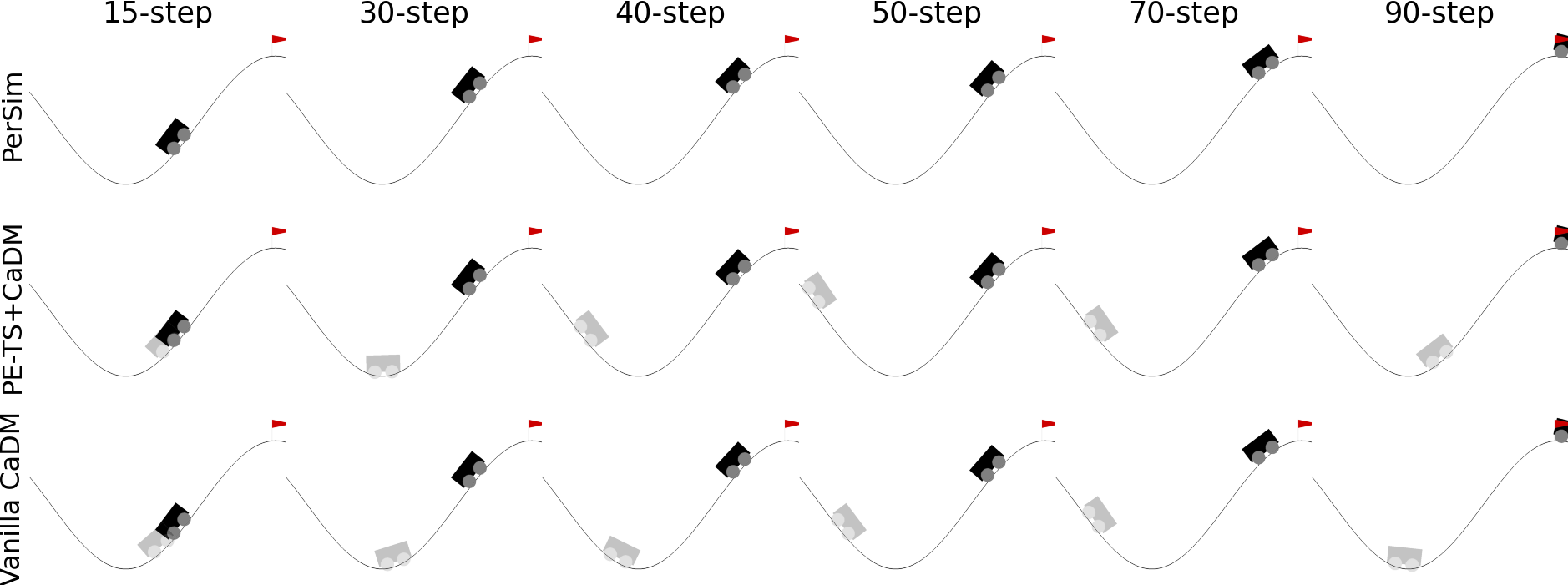
(a) MountainCar with gravity 0.0001

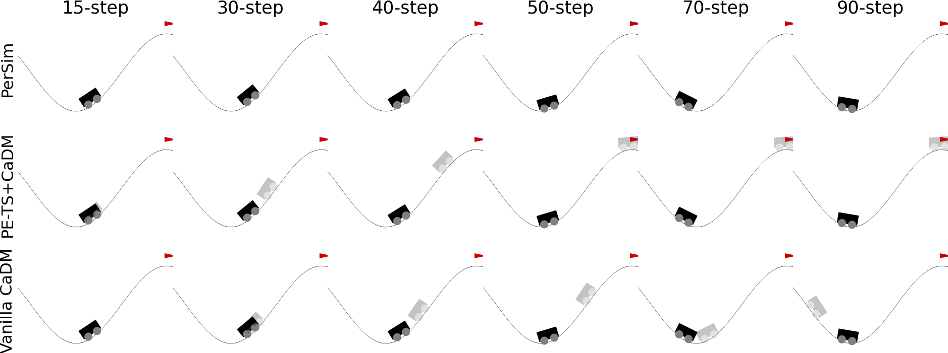
(b) MountainCar with gravity 0.0025

(c) CartPole with pole length 0.85

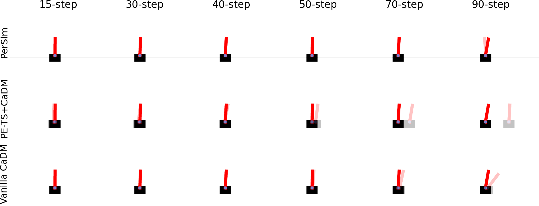
(d) CartPole with pole length 0.5

Figure 4: Visualization of the prediction accuracy of PerSim for two heterogeneous agents in MountainCar and CartPole, and how it compares with the two CaDM variants. Specifically, given an initial state and a sequence of actions, we predict future states for the next 90 steps. Ground-truth states and predicted states are denoted by the opaque and translucent objects, respectively.

F.2 Detailed Average Reward Results

In this section, we show the full results for the experiments for the reward achieved in each environment. Specifically, we report the average reward achieved by PerSim and several state-of-the-art model-based and model-free offline RL methods on the three benchmark environments across 5 trials. We evaluate the performance of each method using the average reward over 20 episodes for the model-based methods and the average reward over 100 episodes for the model-free methods. We repeat each experiment five times and report the mean and standard deviation.

The results are summarized in Tables 9, 10, and 11 for MountainCar, CartPole, and HalfCheetah, respectively.

Table 9: Average Reward: MountainCar

Data	Method	Agent 1	Agent 2	Agent 3	Agent 4	Agent 5
		0.0001	0.0005	0.001	0.0025	0.0035
Pure	PerSim	-56.80$\pm$1.83	-74.30$\pm$6.59	-114.1$\pm$16.1	-189.4$\pm$6.44	-210.6$\pm$4.27
	Vanilla CaDM	-106.3$\pm$44.1	-289.8$\pm$195	-332.8$\pm$193	-432.3$\pm$117	-471.8$\pm$43.0
	PE-TS CaDM	-74.23$\pm$16.5	-119.1$\pm$44.4	-361.3$\pm$240	-492.3$\pm$13.3	-500.0$\pm$0.0
	BCQ-P	-67.60$\pm$22.3	-68.60$\pm$19.6	-79.20$\pm$14.7	-267.8$\pm$202	-295.1$\pm$180
	BCQ-A	-44.79$\pm$0.08	-50.50$\pm$0.40	-63.52$\pm$0.19	-380.7$\pm$170	-500.0$\pm$0.0
	CQL-P	-176.1$\pm$45.2	-161.8$\pm$40.6	-166.1$\pm$33.9	-316.4$\pm$26.4	-362.9$\pm$17.9
	CQL-A	-44.60$\pm$0.0	-49.70$\pm$0.0	-63.30$\pm$0.3	-500.0$\pm$0.0	-499.3$\pm$0.7
	MOReL-P	-46.00$\pm$1.1	-53.20$\pm$3.3	-220.3$\pm$162.6	-500.0$\pm$0.0	-500.0$\pm$0.0
	MOReL-A	-373.0$\pm$33.5	-488.8$\pm$4.9	-499.4$\pm$0.2	-500.0$\pm$0.0	-500.0$\pm$0.0
Random	PerSim	-57.70$\pm$5.63	-74.30$\pm$6.39	-120.4$\pm$2.17	-186.6$\pm$4.25	-210.1$\pm$4.48
	Vanilla CaDM	-62.57$\pm$5.11	-75.27$\pm$4.59	-274.9$\pm$74.2	-479.3$\pm$21.7	-497.5$\pm$4.39
	PE-TS CaDM	-82.00$\pm$3.47	-115.7$\pm$7.63	-472.1$\pm$48.3	-500.0$\pm$0.0	-500.0$\pm$0.0
	BCQ-P	-500.0$\pm$0.0	-500.0$\pm$0.0	-500.0$\pm$0.0	-500.0$\pm$0.0	-500.0$\pm$0.0
	BCQ-A	-500.0$\pm$0.0	-500.0$\pm$0.0	-500.0$\pm$0.0	-500.0$\pm$0.0	-500.0$\pm$0.0
	CQL-P	-500.0$\pm$0.0	-500.0$\pm$0.0	-500.0$\pm$0.0	-500.0$\pm$0.0	-500.0$\pm$0.0
	CQL-A	-500.0$\pm$0.0	-500.0$\pm$0.0	-500.0$\pm$0.0	-500.0$\pm$0.0	-500.0$\pm$0.0
	MOReL-P	-45.00$\pm$0.3	-50.40$\pm$0.5	-68.20$\pm$5.4	-500.0$\pm$0.0	-500.0$\pm$0.0
	MOReL-A	-495.0$\pm$3.9	-480.6$\pm$3.1	-500.0$\pm$0.0	-500.0$\pm$0.0	-500.0$\pm$0.0
Pure-$\varepsilon$-20	PerSim	-54.20$\pm$0.56	-67.80$\pm$0.48	-111.7$\pm$6.20	-191.2$\pm$6.70	-199.7$\pm$3.99
	Vanilla CaDM	-56.73$\pm$4.20	-70.70$\pm$1.54	-148.7$\pm$11.6	-463.2$\pm$57.5	-478.9$\pm$35.8
	PE-TS CaDM	-107.6$\pm$36.3	-158.5$\pm$84.3	-464.6$\pm$37.3	-500.0$\pm$0.0	-500.0$\pm$0.0
	BCQ-P	-71.21$\pm$24.4	-72.10$\pm$20.5	-78.41$\pm$14.3	-286.6$\pm$196	-328.3$\pm$158
	BCQ-A	-364.5$\pm$180	-435.7$\pm$63.7	-282.7$\pm$308	-260.6$\pm$51.4	-204.5$\pm$68.9
	CQL-P	-79.40$\pm$16.1	-78.80$\pm$13.9	-86.50$\pm$10.8	-357.9$\pm$12.5	-407.6$\pm$15.3
	CQL-A	-44.70$\pm$0.1	-49.70$\pm$0.0	-63.30$\pm$0.2	-500.0$\pm$0.0	-500.0$\pm$0.0
	MOReL-P	-83.50$\pm$15.6	-81.70$\pm$14.2	-88.60$\pm$11.1	-357.0$\pm$13.8	-407.4$\pm$17.1
	MOReL-A	-44.60$\pm$0.1	-49.70$\pm$0.0	-63.30$\pm$0.2	-500.0$\pm$0.0	-500.0$\pm$0.0
Pure-$\varepsilon$-40	PerSim	-54.60$\pm$0.55	-71.10$\pm$1.89	-115.7$\pm$4.80	-189.7$\pm$7.14	-200.3$\pm$2.26
	Vanilla CaDM	-55.23$\pm$0.76	-67.90$\pm$7.30	-163.7$\pm$30.8	-481.7$\pm$25.3	-496.2$\pm$4.31
	PE-TS CaDM	-102.3$\pm$20.3	-120.7$\pm$18.8	-476.0$\pm$41.5	-500.0$\pm$0.0	-500.0$\pm$0.0
	BCQ-P	-50.01$\pm$7.50	-57.10$\pm$10.3	-66.11$\pm$3.91	-373.6$\pm$180	-352.0$\pm$211
	BCQ-A	-94.87$\pm$0.88	-80.03$\pm$38.5	-329.6$\pm$242	-358.7$\pm$201	-486.5$\pm$20.6
	CQL-P	-61.40$\pm$2.1	-64.90$\pm$2.1	-75.10$\pm$1.2	-366.9$\pm$21.3	-429.1$\pm$18.8
	CQL-A	-44.70$\pm$0.0	-49.70$\pm$0.0	-63.30$\pm$0.4	-500.0$\pm$0.0	-490.1$\pm$9.6
	MOReL-P	-61.30$\pm$2.3	-65.80$\pm$1.2	-75.00$\pm$1.4	-373.2$\pm$19.3	-428.5$\pm$21.0
	MOReL-A	-44.70$\pm$0.0	-49.70$\pm$0.0	-63.30$\pm$0.4	-500.0$\pm$0.0	-492.1$\pm$9.3
	True env+MPC	-53.95$\pm$4.10	-72.43$\pm$7.80	-110.8$\pm$23.8	-182.9$\pm$22.9	-197.5$\pm$20.7

Table 10: Average Reward: CartPole

Data	Method	Agent 1	Agent 2	Agent 3	Agent 4	Agent 5
		(2/0.5)	(10.0/0.5)	(18.0/0.5)	(10/0.85)	(10/0.15)
Pure	PerSim	199.7$\pm$0.58	198.7$\pm$0.86	198.5$\pm$1.16	193.8$\pm$4.28	192.0$\pm$2.28
	Vanilla CaDM	168.0$\pm$19.7	197.7$\pm$1.50	173.6$\pm$6.10	190.8$\pm$6.80	58.10$\pm$10.7
	PE-TS CaDM	92.30$\pm$44.8	200.0$\pm$0.0	200.0$\pm$0.0	193.6$\pm$8.30	127.5$\pm$9.50
	BCQ-P	166.2$\pm$39.3	187.4$\pm$14.7	187.2$\pm$15.0	181.2$\pm$13.5	182.8$\pm$15.0
	BCQ-A	65.40$\pm$67.5	138.0$\pm$80.3	79.20$\pm$79.9	79.20$\pm$69.5	132.1$\pm$85.0
	CQL-P	154.4$\pm$17.7	190.8$\pm$1.2	193.9$\pm$1.7	190.9$\pm$0.7	170.2$\pm$0.6
	CQL-A	122.8$\pm$63.4	189.4$\pm$6.6	199.3$\pm$0.7	179.4$\pm$20.6	193.6$\pm$5.4
	MOReL-P	35.80$\pm$1.4	90.40$\pm$26.2	94.20$\pm$25.1	96.60$\pm$24.1	66.40$\pm$24.5
	MOReL-A	33.70$\pm$3.8	16.00$\pm$6.5	16.20$\pm$0.6	27.50$\pm$0.1	10.10$\pm$0.7
Random	PerSim	197.7$\pm$7.82	189.5$\pm$4.28	190.3$\pm$4.74	193.0$\pm$6.60	185.7$\pm$3.49
	Vanilla CaDM	150.5$\pm$15.7	158.7$\pm$17.1	161.4$\pm$15.8	175.6$\pm$5.80	65.10$\pm$16.3
	PE-TS CaDM	88.60$\pm$18.5	194.0$\pm$2.00	197.6$\pm$2.20	196.1$\pm$3.00	171.0$\pm$21.7
	BCQ-P	44.80$\pm$34.0	58.21$\pm$58.0	56.92$\pm$56.0	57.91$\pm$53.0	36.40$\pm$36.0
	BCQ-A	43.90$\pm$16.4	18.70$\pm$13.1	7.200$\pm$0.84	21.10$\pm$5.81	39.50$\pm$12.1
	CQL-P	39.90$\pm$29.9	72.30$\pm$41.7	67.80$\pm$44.4	77.90$\pm$26.2	148.7$\pm$17.1
	CQL-A	67.40$\pm$49.1	9.300$\pm$0.1	16.30$\pm$9.9	30.60$\pm$26.4	7.000$\pm$1.9
	MOReL-P	50.20$\pm$7.9	59.10$\pm$17.8	57.80$\pm$17.8	68.90$\pm$17.4	40.40$\pm$12.4
	MOReL-A	35.80$\pm$0.4	20.70$\pm$1.0	14.30$\pm$1.4	27.50$\pm$0.7	10.60$\pm$0.2
Pure-$\varepsilon$-20	PerSim	199.8$\pm$0.24	200.0$\pm$0.0	200.0$\pm$0.0	199.1$\pm$1.3	197.8$\pm$1.68
	Vanilla CaDM	171.1$\pm$38.1	195.3$\pm$3.00	180.7$\pm$4.30	193.4$\pm$2.10	64.20$\pm$10.0
	PE-TS CaDM	98.30$\pm$42.9	199.6$\pm$0.50	199.0$\pm$1.40	198.6$\pm$0.40	141.1$\pm$12.0
	BCQ-P	98.90$\pm$30.2	170.9$\pm$19.0	163.0$\pm$36.5	162.1$\pm$15.5	86.10$\pm$72.1
	BCQ-A	67.30$\pm$62.2	130.0$\pm$76.1	33.40$\pm$0.62	65.60$\pm$51.8	140.0$\pm$80.6
	CQL-P	163.7$\pm$13.6	197.4$\pm$2.9	198.6$\pm$2.4	198.1$\pm$2.6	190.4$\pm$6.6
	CQL-A	42.40$\pm$11.9	189.8$\pm$10.2	22.20$\pm$20.0	199.0$\pm$1.9	199.8$\pm$0.2
	MOReL-P	166.7$\pm$13.6	197.0$\pm$3.1	198.3$\pm$2.6	197.7$\pm$2.7	189.4$\pm$7.1
	MOReL-A	41.40$\pm$13.1	188.3$\pm$11.0	20.00$\pm$21.9	198.8$\pm$2.1	199.9$\pm$0.2
Pure-$\varepsilon$-40	PerSim	199.9$\pm$0.18	199.8$\pm$0.20	199.3$\pm$1.34	198.0$\pm$1.21	197.4$\pm$1.72
	Vanilla CaDM	160.6$\pm$46.6	197.3$\pm$1.50	194.9$\pm$3.70	191.9$\pm$6.40	79.60$\pm$31.6
	PE-TS CaDM	91.90$\pm$67.6	199.8$\pm$0.20	200.0$\pm$0.0	197.0$\pm$1.40	143.5$\pm$17.5
	BCQ-P	28.90$\pm$6.80	24.97$\pm$12.8	27.90$\pm$25.9	31.80$\pm$25.9	18.50$\pm$11.1
	BCQ-A	34.60$\pm$1.55	23.20$\pm$17.8	7.180$\pm$0.76	47.71$\pm$48.7	23.20$\pm$9.44
	CQL-P	182.2$\pm$18.0	197.4$\pm$4.6	198.9$\pm$2.1	198.3$\pm$2.9	191.9$\pm$8.7
	CQL-A	20.70$\pm$0.7	25.70$\pm$14.3	15.30$\pm$7.3	134.2$\pm$10.2	9.700$\pm$8.1
	MOReL-P	178.9$\pm$18.7	196.8$\pm$5.0	198.7$\pm$2.3	197.9$\pm$3.1	190.6$\pm$9.3
	MOReL-A	20.70$\pm$0.8	23.90$\pm$15.5	16.60$\pm$7.6	135.4$\pm$11.2	10.80$\pm$8.8
	True env+MPC	200.0$\pm$0.0	200.0$\pm$0.0	200.0$\pm$0.0	198.4$\pm$7.20	200.0$\pm$0.0

Table 11: Average Reward: HalfCheetah

Data	Method	Agent 1	Agent 2	Agent 3	Agent 4	Agent 5
		(0.3/1.7)	(1.7/0.3)	(0.3/0.3)	(1.7/1.7)	(1.0/1.0)
Pure	PerSim	1984 $\pm$763	997.0$\pm$403	714.7$\pm$314	113.5$\pm$289	1459 $\pm$398
	Vanilla CaDM	50.31$\pm$71.7	-134.0$\pm$81.1	11.39$\pm$171	-169.8$\pm$67.5	331.3$\pm$201
	PE-TS CaDM	481.1$\pm$252	503.7$\pm$181	553.0$\pm$127	246.0$\pm$261	840.1$\pm$383
	BCQ-P	549.8$\pm$322	2006 $\pm$153	-65.18$\pm$92.8	2564 $\pm$70.2	2469 $\pm$67.2
	BCQ-A	-262.7$\pm$96.6	-139.0$\pm$236	165.6$\pm$83.1	1649 $\pm$622	937.2$\pm$221
	CQL-P	-353.5$\pm$78.4	-453.6$\pm$71.9	-476.7$\pm$129	2037 $\pm$294	-145.1$\pm$189
	CQL-A	-65.00$\pm$105	-257.9$\pm$35.9	-279.6$\pm$34.4	689.3$\pm$52.9	301.9$\pm$98.9
	MOReL-P	-1297$\pm$519	-1256 $\pm$627	-1470 $\pm$727	-1175 $\pm$592	-1256 $\pm$608
	MOReL-A	-726.2$\pm$4.9	-666.1$\pm$42.6	-841.7$\pm$39.5	-599.6$\pm$28.2	-688.6$\pm$12.4
Random	PerSim	2124 $\pm$518	2060 $\pm$900	472.0$\pm$56.9	565.2$\pm$377	474.8$\pm$344
	Vanilla CaDM	288.4$\pm$32.4	362.9$\pm$55.4	351.8$\pm$34.9	358.4$\pm$205	475.0$\pm$102
	PE-TS CaDM	754.6$\pm$242	744.5$\pm$281	767.4$\pm$214	555.4$\pm$73.1	2486 $\pm$1488
	BCQ-P	-1.460$\pm$0.16	-1.750$\pm$0.22	-1.690$\pm$0.19	-1.790$\pm$0.21	-1.720$\pm$0.20
	BCQ-A	-498.9$\pm$108	-113.3$\pm$13.0	-159.5$\pm$51.7	-35.73$\pm$7.22	-171.9$\pm$41.5
	CQL-P	-481.5$\pm$25.9	-442.2$\pm$56.4	-672.4$\pm$17.6	-254.5$\pm$39.6	-418.2$\pm$23.4
	CQL-A	-0.700$\pm$0.4	-2.800$\pm$0.8	-0.600$\pm$0.3	-2.000$\pm$0.6	-5.500$\pm$2.0
	MOReL-P	-102.3$\pm$45.7	-188.7$\pm$37.1	-181.0$\pm$67.7	-142.5$\pm$26.8	-141.4$\pm$7.3
	MOReL-A	-430.8$\pm$195	-673.7$\pm$39.3	-365.5$\pm$97.4	-645.5$\pm$53.0	-674.9$\pm$28.9
Pure-$\varepsilon$-20	PerSim	3186 $\pm$604	1032 $\pm$232	1120 $\pm$243	971.2$\pm$916	1666 $\pm$930
	Vanilla CaDM	412.0$\pm$152	31.92$\pm$109	460.2$\pm$159	60.33$\pm$139	166.6$\pm$71.8
	PE-TS CaDM	1082 $\pm$126	1125 $\pm$132	1067 $\pm$64.3	1098 $\pm$344	2843 $\pm$204
	BCQ-P	254.6$\pm$352	406.7$\pm$71.1	385.9$\pm$57.1	-95.34$\pm$65.8	738.0$\pm$512
	BCQ-A	376.8$\pm$102	84.66$\pm$53.3	230.1$\pm$10.0	1180 $\pm$87.3	617.5$\pm$32.6
	CQL-P	838.7$\pm$24.5	3155 $\pm$125	539.9$\pm$313	1479 $\pm$51.0	3561 $\pm$170
	CQL-A	-15.50$\pm$9.0	-73.00$\pm$26.3	-108.0$\pm$64.6	656.9$\pm$181.6	357.6$\pm$110
	MOReL-P	0.600$\pm$210	-171.2$\pm$125	-219.9$\pm$76.7	-106.3$\pm$18.6	-83.60$\pm$110
	MOReL-A	-781.0$\pm$37.9	-613.1$\pm$49.9	-847.1$\pm$64.7	-599.2$\pm$4.6	-702.9$\pm$26.8
Pure-$\varepsilon$-40	PerSim	2590 $\pm$813	1016 $\pm$283	1365 $\pm$582	803.9$\pm$912	724.9$\pm$236
	Vanilla CaDM	465.6$\pm$49.2	452.7$\pm$130	720.0$\pm$74.9	176.7$\pm$359	952.8$\pm$591
	PE-TS CaDM	1500 $\pm$246	1218 $\pm$221	1339 $\pm$54.8	1569 $\pm$306	3094 $\pm$825
	BCQ-P	78.25$\pm$200	173.8$\pm$189	417.1$\pm$155	-56.12$\pm$64.4	55.46$\pm$128
	BCQ-A	269.2$\pm$60.7	-181.5$\pm$57.4	193.0$\pm$31.8	636.4$\pm$137	207.0$\pm$106
	CQL-P	808.5$\pm$240	1662 $\pm$220	-156.3$\pm$119	1416 $\pm$71.8	1908 $\pm$461
	CQL-A	-6.200$\pm$2.9	-386.0$\pm$42.4	37.10$\pm$154	1121 $\pm$95.6	1184 $\pm$604
	MOReL-P	8.500$\pm$61.6	-114.2$\pm$72.2	-195.9$\pm$77.3	-66.60$\pm$7.5	22.60$\pm$28.7
	MOReL-A	-325.9$\pm$17.1	-644.5$\pm$18.8	-798.8$\pm$130	-609.0$\pm$16.8	-711.7$\pm$19.1
	True env+MPC	7459 $\pm$171	42893$\pm$6959	66675$\pm$9364	1746$\pm$624	36344$\pm$7924

F.3 Visualization of Agent Latent Factors

In this section, we visualize the learned agent latent factors associated with the 500 heterogeneous agents in each of the three benchmark environments. Specifically, we visualize the agent latent factors in MountainCar, as we vary the gravity (Figure 5(a)); CartPole, as we vary the pole’s length and the push force (Figures 5(c) and 5(b), respectively); HalfCheetah, as we vary the cheetah’s mass and the joints’ damping (Figures 5(e) and 5(d), respectively).

(a) MountainCar: gravity

(b) CartPole: push force

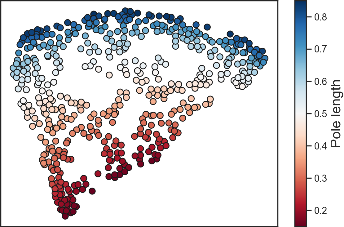
(c) CartPole: pole length

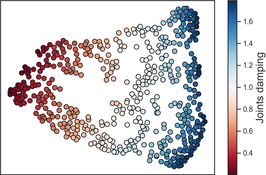
(d) HalfCheetah: joints’ damping

(e) HalfCheetah: links’ mass

Figure 5: t-SNE [48] visualization of the agent latent factors for the 500 heterogeneous agents in MountainCar, CartPole, and HalfCheetah. Colors indicate the value of the modified parameter in each environment (e.g., gravity in MountainCar). These figures demonstrate that the learned latent factors indeed capture the relevant information about the agents heterogeneity in all environments.

F.4 Persim+BCQ/CQL: Experimental details

We evaluate PerSim’s simulation efficacy by quantifying how much the simulated trajectories improve the performance of model-free RL methods such as BCQ and CQL. In particular, we use PerSim to generate synthetic trajectories for each agent of interest to augment the training data available for BCQ/CQL.

We carry out these experiments for the three environments: MountainCar, CartPole, and HalfCheetah. In all environments, as is done in previous experiments (see Section 5.1), we train PerSim using a single observed trajectory from each of the 500 training agents. For these trajectories, the actions are selected randomly, and the covariates of the training agents are selected as described in Section 5.1. Then, we use the trained simulators to produce $5$ synthetic trajectories for each test agent. See Table 4 for information about the test agents in each environment and the range of covariates used for the training agents.

When generating these synthetic trajectories, we use MPC to choose the sequence of actions that maximizes the reward estimated by the simulator, as described in Appendix D.1. We use a horizon $h$ of 50 for MountainCar and CartPole, and a horizon $h$ of 30 for HalfCheetah. The only difference is that instead of choosing the first element from the sequence of actions with the best average reward, we choose the full sequence of actions, and repeat the sampling process until we have a full trajectory.

F.5 Generalizing to Unseen Agents

Setup. In this experiment, we evaluate PerSim’s ability to generalize to unseen agents. An advantage of the factorized approach of PerSim is that the heterogeneity of an agent is captured by its latent agent factors (see Table 5). Hence, the problem of generalizing to unseen agents boils down to accurately estimating the latent agent factors. To estimate these latent agent factors, we assume access to the covariates of the unseen agents, as well as a fraction $1\geq p>0$ of the covariates of the training agents. With access to this information, we propose the following natural two-step procedure to estimate the latent agent factor: (1) Use a supervised learning method to learn a mapping between the (available) training agent covariates and the learned agent-specific latent factor in PerSim (see Figure 1); (2) Apply this mapping on the covariate data of an unseen test agent to estimate its latent agent factor, which is sufficient to build a personalized simulator for it.

We conduct this experiment for MountainCar, where we train PerSim using 500 agents, each with a gravity value selected uniformly at random from the range $[0.0001,0.0035]$. We then evaluate PerSim’s performance on 5 unseen agents selected as follow:

1. One unseen agent from the training range $[0.0001,0.0035]$. Specifically, the one with gravity $0.002$.

2. Two agents outside the lower end of the range with gravity of $0.00008$ and $0.00005$.

3. Two agents outside the upper end of the range with gravity of $0.0037$, and $0.004$.

We first train PerSim on trajectories generated from the aforementioned 500 training agents, and carry out the experiments for trajectories generated via the random and pure policies. Then, we learn a mapping between the learned agent factors and covariates through an MLP with 2 hidden-layers each with 64 units. We assume access to a fraction $p\in\{1.0,0.5,0.25,0.1\}$ of the covariates to train this function. We report PerSim’s efficacy through the same two metrics we used before: prediction error and average reward for the five unseen agents.

Results. As Table 12 shows, in terms of prediction error, PerSim outperforms both Vanilla CaDM and PE-TS CaDM in both the random and pure datasets for all unseen test agents. Further, Table 13 shows that PerSim achieves the best reward among the three baselines (BCQ-P, Vanilla CaDM and PE-TS CaDM) for most unseen test agents. Pleasingly, these results are consistent as we vary $p\in\{1.0,0.5,0.25,0.1\}$. That is, even with access to only $10\%$ of the covariates of the training agents (i.e., $p=0.1$), PerSim is able to simulate the unseen agents well. Note that PerSim is trained without access to any of the latent covariates (e.g., gravity in MountainCar), but to generalize to unseen agents, it requires access to some of the covariates to learn the mapping between these covariates and the latent agent factors. It is important to note that PerSim utilizes explicit knowledge of the covariates of the unseen test agents (and a subset of the training agents), which these other methods do not do in their current implementations. Indeed, it is our latent factor representation (in particular, the agent-specific latent factors) which seamlessly allows us to utilize these covariates to build simulators for the unseen agents.

Table 12: Prediction Error: MountainCar, Unseen Agents

Data	Method	Agent 1	Agent 2	Agent 3	Agent 4	Agent 5
		0.00005	0.00008	0.002	0.0037	0.004
Random	PerSim(p=1.0)	0.004 (1.00)	0.004 (1.00)	0.000 (1.00)	0.001 (1.00)	0.002 (1.00)
	PerSim(p=0.5)	0.007 (0.99)	0.006 (0.99)	0.000 (1.00)	0.001 (1.00)	0.001 (1.00)
	PerSim(p=0.25)	0.005 (0.99)	0.004 (1.00)	0.000 (1.00)	0.001 (1.00)	0.001 (1.00)
	PerSim(p=0.1)	0.005 (0.99)	0.005 (0.99)	0.000 (1.00)	0.000 (1.00)	0.000 (1.00)
	Vanilla CaDM	0.378 (0.13)	0.373 (0.12)	0.159 (0.13)	0.329 (0.16)	0.339 (0.15)
	PE-TS CaDM	0.399 (0.06)	0.351 (0.08)	0.176 (0.07)	0.193 (0.04)	0.214 (0.05)
Pure	PerSim(p=1.0)	0.192 (0.99)	0.183 (0.98)	0.029 (0.86)	0.029 (0.90)	0.034 (0.88)
	PerSim(p=0.5)	0.039 (0.98)	0.052 (0.99)	0.029 (0.84)	0.030 (0.89)	0.036 (0.86)
	PerSim(p=0.25)	0.061 (0.98)	0.479 (0.98)	0.029 (0.88)	0.034 (0.87)	0.039 (0.84)
	PerSim(p=0.1)	0.043 (0.98)	0.046 (0.98)	0.033 (0.83)	0.029 (0.90)	0.034 (0.88)
	Vanilla CaDM	0.213 (0.05)	0.204 (0.04)	0.199 (0.04)	0.357 (0.03)	0.362 (0.03)
	PE-TS CaDM	0.432 (0.07)	0.450 (0.09)	0.187 (0.04)	0.230 (0.06)	0.232 (0.07)

Table 13: Average Reward: MountainCar, Unseen Agents

Data	Method	Agent 1	Agent 2	Agent 3	Agent 4	Agent 5
		0.00005	0.00008	0.002	0.0037	0.004
Random	PerSim(p=1.0)	-53.82$\pm$0.41	-53.97$\pm$0.35	-188.7$\pm$6.46	-202.6$\pm$2.69	-200.2$\pm$0.74
	PerSim(p=0.5)	-53.98$\pm$0.93	-54.57$\pm$0.39	-192.3$\pm$3.61	-207.8$\pm$2.53	-204.0$\pm$1.15
	PerSim(p=0.25)	-53.77$\pm$0.33	-54.22$\pm$0.88	-196.4$\pm$4.48	-206.4$\pm$5.45	-209.9$\pm$5.33
	PerSim(p=0.1)	-53.25$\pm$0.56	-54.23$\pm$1.05	-198.2$\pm$1.38	-207.3$\pm$0.86	-208.6$\pm$3.40
	Vanilla CaDM	-102.4$\pm$15.6	-97.17$\pm$20.6	-500.0$\pm$0.0	-500.0$\pm$0.0	-500.0$\pm$0.0
	PE-TS CaDM	-82.60$\pm$20.2	-96.07$\pm$5.10	-500.0$\pm$0.0	-500.0$\pm$0.0	-500.0$\pm$0.0
	BCQ-P	-500.0$\pm$0.0	-500.0$\pm$0.0	-500.0$\pm$0.0	-500.0$\pm$0.0	-500.0$\pm$0.0
Pure	PerSim(p=1.0)	-75.17$\pm$12.8	-74.73$\pm$11.4	-179.3$\pm$4.74	-203.7$\pm$4.13	-201.4$\pm$5.72
	PerSim(p=0.5)	-79.83$\pm$14.9	-79.40$\pm$13.9	-181.9$\pm$2.02	-206.7$\pm$6.51	-201.6$\pm$4.67
	PerSim(p=0.25)	-77.28$\pm$13.4	-77.73$\pm$19.7	-178.4$\pm$2.77	-199.7$\pm$3.41	-209.1$\pm$4.83
	PerSim(p=0.1)	-85.08$\pm$22.7	-90.42$\pm$19.6	-183.0$\pm$1.40	-204.2$\pm$6.48	-203.0$\pm$5.12
	Vanilla CaDM	-52.63$\pm$1.05	-54.90$\pm$2.60	-446.8$\pm$51.2	-494.1$\pm$9.30	-494.1$\pm$10.3
	PE-TS CaDM	-60.17$\pm$2.66	-63.43$\pm$4.80	-374.4$\pm$77.3	-500.0$\pm$0.0	-500.0$\pm$0.0
	BCQ-P	-184.9$\pm$170	-183.1$\pm$170	-277.6$\pm$183	-322.7$\pm$146	-333.7$\pm$139

F.6 Robustness to Data Scarcity

Setup. In this experiment, we address the robustness of PerSim to data scarcity. In particular, we decrease the number of observed agents from $N=250$ to $N=25$ in all three benchmarking environments. As is done in previous experiments, we compare with the two variants of CaDM and BCQ, and evaluate the performance on five test agents. We use trajectories generated by a random policy in MountainCar and HalfCheetah, and pure policy for CartPole. We use a pure policy for CartPole to ensure that each trajectory is not too short (see Table 5 for the average length of a trajectory in each environment under different policies). We perform these experiments five times, where in each time, the agent covariates are re-sampled from the covariates range. We report the average reward across the five trials and the corresponding standard deviations.

Results. We report the average reward achieved by PerSim and baselines in Tables 14, 15 and 16 for MountainCar, CartPole, and HalfCheetah, respectively. As demonstrated in the tables, even when we vary the number of trajectories, PerSim consistently achieves a higher reward than the other baselines across all agents in MountainCar and CartPole. In HalfCheetah, PerSim and PE-TS CaDM perform the best among the baselines. One thing to note is the high variance in HalfCheetah experiments, across all baselines, indicating the fundamental challenge faced when dealing with environments with both high-dimensional state space and limited data. Addressing such a challenge remains an interesting direction for future work.

Table 14: Average Reward: MountainCar with different number of training agents.

Data	N	Method	Agent 1	Agent 2	Agent 3	Agent 4	Agent 5
			0.0001	0.0005	0.001	0.0025	0.0035
Random	250	PerSim	-53.70$\pm$0.41	-66.50 $\pm$1.21	-116.6$\pm$3.18	-192.3$\pm$1.23	-199.6$\pm$3.40
		Vanilla CaDM	-59.90$\pm$1.61	-78.13$\pm$7.11	-332.6$\pm$41.3	-467.8$\pm$16.2	-500.0$\pm$0.0
		PE-TS CaDM	-73.66$\pm$3.15	-106.8$\pm$7.15	-473.8$\pm$37.0	-500.0$\pm$0.0	-500.0$\pm$0.0
		BCQ-P	-500.0$\pm$0.0	-500.0$\pm$0.0	-500.0$\pm$0.0	-500.0$\pm$0.0	-500.0$\pm$0.0
Random	100	PerSim	-55.00$\pm$0.70	-67.02$\pm$1.76	-110.3$\pm$3.46	-193.1$\pm$5.21	-197.4$\pm$3.05
		Vanilla CaDM	-66.00$\pm$5.06	-83.10$\pm$8.64	-307.1$\pm$96.2	-486.3$\pm$23.7	-500.0$\pm$0.0
		PE-TS CaDM	-79.33$\pm$4.36	-106.5$\pm$19.3	-418.4$\pm$27.3	-492.7$\pm$10.3	-499.9$\pm$0.14
		BCQ-P	-500.0$\pm$0.0	-500.0$\pm$0.0	-500.0$\pm$0.0	-500.0$\pm$0.0	-500.0$\pm$0.0
Random	50	PerSim	-54.20$\pm$0.90	-66.40$\pm$0.17	-110.2$\pm$8.65	-188.7$\pm$5.25	-199.6$\pm$3.23
		Vanilla CaDM	-58.80$\pm$1.40	-66.37$\pm$0.35	-131.8$\pm$17.6	-497.2$\pm$4.85	-500.0$\pm$0.0
		PE-TS CaDM	-67.86$\pm$7.15	-79.73$\pm$6.37	-290.5$\pm$76.9	-458.4$\pm$26.8	-498.5$\pm$2.12
		BCQ-P	-214.3$\pm$202	-348.6$\pm$186	-428.1$\pm$103	-500.0$\pm$0.0	-500.0$\pm$0.0
Random	25	PerSim	-56.80$\pm$1.81	-67.50$\pm$2.81	-139.9$\pm$29.5	-246.8$\pm$39.1	-243.8$\pm$47.1
		Vanilla CaDM	-62.33$\pm$3.34	-76.80$\pm$10.9	-275.7$\pm$63.9	-473.0$\pm$24.1	-496.5$\pm$4.90
		PE-TS CaDM	-67.26$\pm$6.95	-86.96$\pm$10.9	-331.0$\pm$121	-497.9$\pm$2.92	-500.0$\pm$0.0
		BCQ-P	-500.0$\pm$0.0	-500.0$\pm$0.0	-500.0$\pm$0.0	-500.0$\pm$0.0	-500.0$\pm$0.0

Table 15: Average Reward: CartPole with different number of training agents.

Data	N	Method	Agent 1	Agent 2	Agent 3	Agent 4	Agent 5
			(2/0.5)	(10.0/0.5)	(18.0/0.5)	(10/0.85)	(10/0.15)
Pure	250	PerSim	200.0$\pm$0.0	198.6$\pm$1.96	197.3$\pm$3.82	198.3$\pm$1.45	196.4$\pm$5.11
		Vanilla	132.7$\pm$15.1	192.8$\pm$1.69	191.9$\pm$2.59	186.4$\pm$0.99	65.21$\pm$12.1
		PE-TS CaDM	65.65$\pm$17.0	200.0$\pm$0.0	199.4$\pm$0.90	185.8$\pm$11.8	167.5$\pm$15.7
		BCQ-P	130.2$\pm$1.31	169.6$\pm$21.6	173.3$\pm$7.94	167.3$\pm$8.81	179.6$\pm$2.71
Pure	100	PerSim	200.0$\pm$0.0	199.6$\pm$0.39	199.5$\pm$0.64	197.8$\pm$1.67	197.7$\pm$2.15
		Vanilla CaDM	150.1$\pm$29.3	187.8$\pm$2.67	180.4$\pm$8.08	182.1$\pm$13.5	80.10$\pm$12.8
		PE-TS CaDM	65.66$\pm$23.6	200.0$\pm$0.0	199.9$\pm$0.14	200.0$\pm$0.0	170.0$\pm$21.0
		BCQ-P	90.67$\pm$52.1	49.18$\pm$32.0	119.0$\pm$78.6	108.9$\pm$70.1	81.30$\pm$66.6
Pure	50	PerSim	200.0$\pm$0.0	199.4$\pm$0.87	199.0$\pm$1.34	191.2$\pm$2.87	182.7$\pm$15.1
		Vanilla CaDM	107.8$\pm$6.89	194.68$\pm$3.87	184.3$\pm$2.90	187.3$\pm$8.70	76.46$\pm$14.1
		PE-TS CaDM	96.47$\pm$61.2	200.00$\pm$0.0	196.0$\pm$4.02	192.6$\pm$7.40	152.9$\pm$20.2
		BCQ-P	121.0$\pm$30.0	70.96$\pm$15.8	122.4$\pm$18.6	145.6$\pm$29.0	100.1$\pm$44.2
Pure	25	PerSim	200.0$\pm$0.0	197.3$\pm$3.75	200.0$\pm$0.0	200.0$\pm$0.05	183.5$\pm$6.20
		Vanilla CaDM	108.6$\pm$16.1	190.3$\pm$3.65	187.1$\pm$1.22	185.9$\pm$6.89	56.76$\pm$11.0
		PE-TS CaDM	56.93$\pm$19.9	185.2$\pm$5.02	175.5$\pm$13.9	149.0$\pm$14.9	155.3$\pm$15.1
		BCQ-P	135.9$\pm$4.07	55.27$\pm$47.4	154.7$\pm$9.99	152.5$\pm$16.7	144.9$\pm$25.3

Table 16: Average Reward: HalfCheetah with different number of training agents.

Data	N	Method	Agent 1	Agent 2	Agent 3	Agent 4	Agent 5
			(0.3/1.7)	(1.7/0.3)	(0.3/0.3)	(1.7/1.7)	(1.0/1.0)
Random	250	PerSim	1688$\pm$1093	1415$\pm$1311	703.1$\pm$531	281.0$\pm$309	510.6$\pm$510
		Vanilla CaDM	277.6$\pm$62.6	335.0$\pm$278	240.4$\pm$530	278.9$\pm$98.0	362.2$\pm$124
		PE-TS CaDM	1006$\pm$556	1833$\pm$666	986.2$\pm$211	659.2$\pm$76.3	2303$\pm$571
		BCQ-P	-1.780$\pm$0.36	-1.410$\pm$0.19	-1.830$\pm$0.21	-1.880$\pm$0.25	-1.830$\pm$0.26
Random	100	PerSim	2072$\pm$284	1164$\pm$102	1115$\pm$493	903.3$\pm$398	1058$\pm$219
		Vanilla CaDM	168.9$\pm$154	131.1$\pm$110	93.20$\pm$182	176.5$\pm$131	415.9$\pm$151
		PE-TS CaDM	803.0$\pm$335	657.5$\pm$125	676.0$\pm$244	586.8$\pm$43.2	1484$\pm$934
		BCQ-P	-1.630$\pm$0.08	-1.430$\pm$0.08	-1.770$\pm$0.12	-1.830$\pm$0.10	-1.860$\pm$0.10
Random	50	PerSim	821.9$\pm$529	1984$\pm$58.2	103.0$\pm$122	66.49$\pm$194	701.2$\pm$112
		Vanilla CaDM	236.0$\pm$234	670.0$\pm$167	68.55$\pm$220	248.7$\pm$44.4	802.8$\pm$355
		PE-TS CaDM	496.4$\pm$166	1002$\pm$423	119.6$\pm$62.0	541.4$\pm$180	1895$\pm$989
		BCQ-P	-1.710$\pm$0.28	-1.510$\pm$0.22	-1.800$\pm$0.21	-1.770$\pm$0.26	-1.910$\pm$0.17
Random	25	PerSim	1110$\pm$328	1125$\pm$195	686.4$\pm$352	106.4$\pm$81.1	801.2$\pm$349
		Vanilla CaDM	229.8$\pm$370	187.5$\pm$215	-72.3$\pm$148	206.0$\pm$132	877.0$\pm$449
		PE-TS CaDM	619.9$\pm$271	878.6$\pm$470	84.30$\pm$221	291.3$\pm$258	1464$\pm$913
		BCQ-P	-134.8$\pm$8.40	-210.5$\pm$53.4	-170.0$\pm$14.9	-178.5$\pm$22.9	-87.75$\pm$19.0

References

- [1] A. Agarwal, S. Kakade, A. Krishnamurthy, and W. Sun. Flambe: Structural complexity and representation learning of low rank mdps. arXiv preprint arXiv:2006.10814, 2020.
- [2] A. Agarwal, D. Shah, and D. Shen. Synthetic interventions, 2020.
- [3] R. Agarwal, D. Schuurmans, and M. Norouzi. Striving for simplicity in off-policy deep reinforcement learning. 2019.
- [4] R. Agarwal, D. Schuurmans, and M. Norouzi. An optimistic perspective on offline reinforcement learning. In International Conference on Machine Learning, pages 104–114. PMLR, 2020.
- [5] D. J. Aldous. Representations for partially exchangeable arrays of random variables. Journal of Multivariate Analysis, 11(4):581–598, 1981.
- [6] B. Barak and A. Moitra. Noisy tensor completion via the sum-of-squares hierarchy. In Conference on Learning Theory, pages 417–445. PMLR, 2016.
- [7] Z. I. Botev, D. P. Kroese, R. Y. Rubinstein, and P. L’Ecuyer. The cross-entropy method for optimization. In Handbook of statistics, volume 31, pages 35–59. Elsevier, 2013.
- [8] G. Brockman, V. Cheung, L. Pettersson, J. Schneider, J. Schulman, J. Tang, and W. Zaremba. Openai gym. arXiv preprint arXiv:1606.01540, 2016.
- [9] E. F. Camacho and C. B. Alba. Model predictive control. Springer science & business media, 2013.
- [10] K. Chua, R. Calandra, R. McAllister, and S. Levine. Deep reinforcement learning in a handful of trials using probabilistic dynamics models. arXiv preprint arXiv:1805.12114, 2018.
- [11] I. Clavera, J. Rothfuss, J. Schulman, Y. Fujita, T. Asfour, and P. Abbeel. Model-based reinforcement learning via meta-policy optimization. In Conference on Robot Learning, pages 617–629. PMLR, 2018.
- [12] M. Deisenroth and C. E. Rasmussen. Pilco: A model-based and data-efficient approach to policy search. In Proceedings of the 28th International Conference on machine learning (ICML-11), pages 465–472. Citeseer, 2011.
- [13] C. Finn, P. Abbeel, and S. Levine. Model-agnostic meta-learning for fast adaptation of deep networks. In International Conference on Machine Learning, pages 1126–1135. PMLR, 2017.
- [14] S. Fujimoto, H. Hoof, and D. Meger. Addressing function approximation error in actor-critic methods. In International Conference on Machine Learning, pages 1587–1596. PMLR, 2018.
- [15] S. Fujimoto, D. Meger, and D. Precup. Off-policy deep reinforcement learning without exploration. In International Conference on Machine Learning, pages 2052–2062. PMLR, 2019.
- [16] C. E. Garcia, D. M. Prett, and M. Morari. Model predictive control: Theory and practice—a survey. Automatica, 25(3):335–348, 1989.
- [17] D. Hafner, T. Lillicrap, I. Fischer, R. Villegas, D. Ha, H. Lee, and J. Davidson. Learning latent dynamics for planning from pixels. In International Conference on Machine Learning, pages 2555–2565. PMLR, 2019.
- [18] D. N. Hoover. Relations on probability spaces and arrays of random variables. Preprint, Institute for Advanced Study, Princeton, NJ, 2, 1979.
- [19] M. Janner, J. Fu, M. Zhang, and S. Levine. When to trust your model: Model-based policy optimization. arXiv preprint arXiv:1906.08253, 2019.
- [20] C. Jin, Z. Yang, Z. Wang, and M. I. Jordan. Provably efficient reinforcement learning with linear function approximation. In Conference on Learning Theory, pages 2137–2143. PMLR, 2020.
- [21] L. Kaiser, M. Babaeizadeh, P. Milos, B. Osinski, R. H. Campbell, K. Czechowski, D. Erhan, C. Finn, P. Kozakowski, S. Levine, et al. Model-based reinforcement learning for atari. arXiv preprint arXiv:1903.00374, 2019.
- [22] D. Kalashnikov, A. Irpan, P. Pastor, J. Ibarz, A. Herzog, E. Jang, D. Quillen, E. Holly, M. Kalakrishnan, V. Vanhoucke, et al. Qt-opt: Scalable deep reinforcement learning for vision-based robotic manipulation. arXiv preprint arXiv:1806.10293, 2018.
- [23] R. Kidambi, A. Rajeswaran, P. Netrapalli, and T. Joachims. Morel: Model-based offline reinforcement learning. arXiv preprint arXiv:2005.05951, 2020.
- [24] A. Kumar, J. Fu, M. Soh, G. Tucker, and S. Levine. Stabilizing off-policy q-learning via bootstrapping error reduction. In Advances in Neural Information Processing Systems, pages 11784–11794, 2019.
- [25] A. Kumar, A. Zhou, G. Tucker, and S. Levine. Conservative q-learning for offline reinforcement learning. arXiv preprint arXiv:2006.04779, 2020.
- [26] T. Kurutach, I. Clavera, Y. Duan, A. Tamar, and P. Abbeel. Model-ensemble trust-region policy optimization. arXiv preprint arXiv:1802.10592, 2018.
- [27] S. Lange, T. Gabel, and M. Riedmiller. Batch reinforcement learning. In Reinforcement learning, pages 45–73. Springer, 2012.
- [28] R. Laroche, P. Trichelair, and R. T. Des Combes. Safe policy improvement with baseline bootstrapping. In International Conference on Machine Learning, pages 3652–3661. PMLR, 2019.
- [29] K. Lee, Y. Seo, S. Lee, H. Lee, and J. Shin. Context-aware dynamics model for generalization in model-based reinforcement learning. In International Conference on Machine Learning, pages 5757–5766. PMLR, 2020.
- [30] S. Levine, C. Finn, T. Darrell, and P. Abbeel. End-to-end training of deep visuomotor policies. The Journal of Machine Learning Research, 17(1):1334–1373, 2016.
- [31] S. Levine, A. Kumar, G. Tucker, and J. Fu. Offline reinforcement learning: Tutorial, review, and perspectives on open problems. arXiv preprint arXiv:2005.01643, 2020.
- [32] Y. Liu, A. Swaminathan, A. Agarwal, and E. Brunskill. Provably good batch reinforcement learning without great exploration. arXiv preprint arXiv:2007.08202, 2020.
- [33] Y. Luo, H. Xu, Y. Li, Y. Tian, T. Darrell, and T. Ma. Algorithmic framework for model-based deep reinforcement learning with theoretical guarantees. arXiv preprint arXiv:1807.03858, 2018.
- [34] V. Mnih, K. Kavukcuoglu, D. Silver, A. A. Rusu, J. Veness, M. G. Bellemare, A. Graves, M. Riedmiller, A. K. Fidjeland, G. Ostrovski, et al. Human-level control through deep reinforcement learning. Nature, 518(7540):529, 2015.
- [35] A. Montanari and N. Sun. Spectral algorithms for tensor completion. Communications on Pure and Applied Mathematics, 71(11):2381–2425, 2018.
- [36] A. Nagabandi, I. Clavera, S. Liu, R. S. Fearing, P. Abbeel, S. Levine, and C. Finn. Learning to adapt in dynamic, real-world environments through meta-reinforcement learning. arXiv preprint arXiv:1803.11347, 2018.
- [37] A. Nagabandi, C. Finn, and S. Levine. Deep online learning via meta-learning: Continual adaptation for model-based rl. arXiv preprint arXiv:1812.07671, 2018.
- [38] P. Parmas, C. E. Rasmussen, J. Peters, and K. Doya. Pipps: Flexible model-based policy search robust to the curse of chaos. In International Conference on Machine Learning, pages 4065–4074. PMLR, 2018.
- [39] S. Sæmundsson, K. Hofmann, and M. P. Deisenroth. Meta reinforcement learning with latent variable gaussian processes. arXiv preprint arXiv:1803.07551, 2018.
- [40] J. Schrittwieser, I. Antonoglou, T. Hubert, K. Simonyan, L. Sifre, S. Schmitt, A. Guez, E. Lockhart, D. Hassabis, T. Graepel, et al. Mastering atari, go, chess and shogi by planning with a learned model. Nature, 588(7839):604–609, 2020.
- [41] T. Seno. d3rlpy: An offline deep reinforcement library. https://github.com/takuseno/d3rlpy, 2020.
- [42] D. Shah, D. Song, Z. Xu, and Y. Yang. Sample efficient reinforcement learning via low-rank matrix estimation. arXiv preprint arXiv:2006.06135, 2020.
- [43] D. Shah and C. L. Yu. Iterative collaborative filtering for sparse noisy tensor estimation. In 2019 IEEE International Symposium on Information Theory (ISIT), pages 41–45. IEEE, 2019.
- [44] D. Silver, T. Hubert, J. Schrittwieser, I. Antonoglou, M. Lai, A. Guez, M. Lanctot, L. Sifre, D. Kumaran, T. Graepel, et al. Mastering chess and shogi by self-play with a general reinforcement learning algorithm. arXiv preprint arXiv:1712.01815, 2017.
- [45] D. Silver, J. Schrittwieser, K. Simonyan, I. Antonoglou, A. Huang, A. Guez, T. Hubert, L. Baker, M. Lai, A. Bolton, et al. Mastering the game of go without human knowledge. Nature, 550(7676):354–359, 2017.
- [46] R. S. Sutton. Dyna, an integrated architecture for learning, planning, and reacting. ACM Sigart Bulletin, 2(4):160–163, 1991.
- [47] E. Todorov, T. Erez, and Y. Tassa. Mujoco: A physics engine for model-based control. In 2012 IEEE/RSJ International Conference on Intelligent Robots and Systems, pages 5026–5033. IEEE, 2012.
- [48] L. Van der Maaten and G. Hinton. Visualizing data using t-sne. Journal of machine learning research, 9(11), 2008.
- [49] T. Wang and J. Ba. Exploring model-based planning with policy networks. arXiv preprint arXiv:1906.08649, 2019.
- [50] T. Wang, X. Bao, I. Clavera, J. Hoang, Y. Wen, E. Langlois, S. Zhang, G. Zhang, P. Abbeel, and J. Ba. Benchmarking model-based reinforcement learning. arXiv preprint arXiv:1907.02057, 2019.
- [51] Y. Wu, G. Tucker, and O. Nachum. Behavior regularized offline reinforcement learning. arXiv preprint arXiv:1911.11361, 2019.
- [52] L. Yang and M. Wang. Sample-optimal parametric q-learning using linearly additive features. In International Conference on Machine Learning, pages 6995–7004. PMLR, 2019.
- [53] T. Yu, G. Thomas, L. Yu, S. Ermon, J. Zou, S. Levine, C. Finn, and T. Ma. Mopo: Model-based offline policy optimization. arXiv preprint arXiv:2005.13239, 2020.