Two-flux tunable Aharonov-Bohm caging in a photonic lattice

Abstract

We study the Aharonov-Bohm caging effect in a one-dimensional lattice of theta-shaped units defining a chain of interconnected plaquettes, each one threaded by two synthetic flux lines. In the proposed system, light trapping results from the destructive interference of waves propagating along three arms, this implies that the caging effect is tunable and it can be controlled by changing the tunnel couplings $J$. These features reflect on the diffraction pattern allowing to establish a clear connection between the lattice topology and the resulting AB interference.

I Introduction

In the early 1980s the geometrical interpretation of some phenomenological observables has introduced a new paradigm for the explanation of different effectsVanderbilt (2018), modifying, for example, our view of non-relativistic quantum phenomena such as the quantum Hall effect Thouless et al. (1982) and prompting new developments and discoveries of paramount relevance ranging from modern polarization theoryResta (1993) to topological phasesHasan and Kane (2010).

Nowadays, the geometry of the Hilbert space, with its metric, defining the distance between two quantum states, and its connectionWilczek and Shapere (1989), fixing the phase accumulated along quantum trajectories, is a central object in condensed matter research, holding great promises for quantum information applications. In photonics and atomic physics the quest to engineer and control the geometric and topological properties of artificial lattices fostered remarkable efforts to implement effective electromagnetic fields for neutral particles.Aidelsburger, Nascimbene, and Goldman (2018) Just to mention a few examples, uniform magnetic fields were achieved in optical lattice-based experiments,Aidelsburger et al. (2011) in ring resonator arrays Hafezi et al. (2013), in optomechanical systems Schmidt et al. (2015). In photonic lattices, artificial gauge fields were generated using different techniques, i.e. introducing topological defects in two-dimensonal structures,Rechtsman et al. (2012); Lumer et al. (2019) applying time-dependent modulationFang, Yu, and Fan (2012a); Goldman and Dalibard (2014); Jörg et al. (2017), employing synthetic modal dimensionsLustig et al. (2019) and, very recently, controlling the orbital angular momentum of the input light beam.Jörg et al. (2020) What underlies most of the observations carried out in the above systems is the first discovered and most basic consequence of the existence of gauge-fields, the Aharonov-Bohm (AB) effect Aharonov and Bohm (1959). The paramount importance of this effect ranges from metrological applications to basic physicsBatelaan and Tonomura (2009). It is a non-local effect, arising from the interference of electron beams traveling along paths enclosing a magnetic flux. As first recognized by Wu and Yang Wu and Yang (1975), it naturally leads to the concept of path-dependent phase factor as a basis to describe electromagnetism and gauge theories in general. Furthermore, as it clearly emerges in path-integral derivations, AB interference reflects the multiply connected nature of the space and it may have impressive consequences on transport. An example is Aharonov-Bohm caging a single-particle localization effect arising from the interplay between the lattice structure and the magnetic flux, first predicted by J. Vidal et al. Vidal, Mosseri, and Douçot (1998) for two-dimensional electronic lattices and subsequently extended and experimentally verified in different contexts, Leykam, Andreanov, and Flach (2018); Abilio et al. (1999); Rizzi, Cataudella, and Fazio (2006) including photonic lattices, see e.g. Refs. Fang, Yu, and Fan, 2012a; Mukherjee et al., 2018; Kremer et al., 2020.

In the present work we study the propagation of light through a one-dimensional array of theta-shaped plaquettes threaded by two fluxes as shown in Fig. 1, that, for brevity, we call $\theta$-lattice. The presence of two fluxes allows us to investigate in a simple but non-trivial framework the signatures of Aharonov-Bohm interference on diffraction patterns highlighting its topological significance and showing how in this case the caging effect becomes fully tunable.

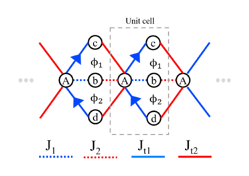
Figure 1: Sketch of the structure of the $\theta$-lattice composed of interconnected plaquettes, each one threaded by two synthetic flux lines, $\phi_{1}$ and $\phi_{2}$. An arrow means a phase $e^{i\phi}$.

II Model

We consider a one-dimensional lattice of theta-shaped units as shown in Fig.1. Its unit cell consists of four sites indicated respectively as $A$, $b$, $c$ and $d$. The three arms of each ring, defined by the sites $A_{n}$, $A_{n+1}$ and respectively $b_{n}$, $c_{n}$ and $d_{n}$, enclose two synthetic flux lines, indicated respectively as $\phi_{1}$ and $\phi_{2}$.
The Hamiltonian of the $\theta$-lattice can thus be written as:

$$H = \sum_{n}\left[J_{\rm t1}\left(a^{\dagger}_{n}c_{n}e^{-i\phi_{1}}+a^{\dagger}_{n}d_{n}e^{i\phi_{2}}\right)+J_{\rm t2}\left(a^{\dagger}_{n}d_{n-1}+a^{\dagger}_{n}c_{n-1}\right)+\right.$$ (1)

$$\left.+J_{1}a^{\dagger}_{n}b_{n}+J_{2}a^{\dagger}_{n}b_{n-1}+{\rm H.c.}\right]$$

where $m_{n}$, $m^{\dagger}_{n}$ with $m=a,\,b,\,c,\,d$ are bosonic annihilation and creation operators corresponding to the sites $A,\,b,\,c,\,d$ of the cell $n$. Switching to $k$-space we obtain:

$$\mathcal{H}(k,\phi_{1},\phi_{2}) = \sum_{k}\big{[}J_{b}(k)\,a^{\dagger}_{k}b_{k}+J_{c}(k,\phi_{1})\,a^{\dagger}_{k}c_{k}+$$ (2)

$$J_{d}(k,\phi_{2})\,a^{\dagger}_{k}d_{k}+{\rm H.c.}\big{]}$$

where $m_{k}=\frac{1}{\sqrt{N}}\sum_{n}m_{n}e^{ikn}$, with $N$ denoting the number of unit cells in the lattice, while $J_{b}(k)=J_{1}+J_{2}e^{-ik}$ and $J_{c}(k,\phi)=J_{d}(k,-\phi)=J_{t1}e^{-i\phi}+J_{t2}e^{-ik}$, where $J_{1}$ and $J_{t1}$ and $J_{2}$ and $J_{t2}$ denote the intra- and inter-cell hopping amplitudes. The $\phi_{1}$, $\phi_{2}$ dependence of $J_{c}$ and $J_{d}$ is due to the presence of the synthetic gauge fields. We note that setting $J_{t2}=J_{t1}=0$ the $\theta$-lattice reduces to the non-abelian Lieb lattice modelBrosco et al. (2020) while setting $J_{b}=0$ it reduces to the standard rhombi chain with a flux $\phi_{T}=\phi_{1}+\phi_{2}$.

The Hamiltonian $\mathcal{H}(k,\phi_{1},\phi_{2})$ is invariant, up to a gauge transformation, under permutations of the three arms b, c, and d, i.e. under elements of the non-Abelian group $S_{3}$. This implies that the state

$$|\phi_{s}(k)\rangle=J_{b}|b_{k}\rangle+J_{c}|c_{k}\rangle+J_{d}|d_{k}\rangle,$$ (3)

invariant under elements of $S_{3}$, yields two dispersive modes:

$$|\psi_{\pm}(k)\rangle=\frac{1}{\sqrt{2}}\left[|a_{k}\rangle\pm\frac{|\phi_{s}(k)\rangle}{\Delta(k,\phi_{1},\phi_{2})}\right]$$ (4)

with longitudinal momenta $\kappa_{\pm}(k,\phi_{1},\phi_{2})=\pm\Delta(k,\phi_{1},\phi_{2})$ and

$$\Delta(k,\phi_{1},\phi_{2})=\sqrt{|J_{b}(k)|^{2}+|J_{c}(k,\phi_{1})|^{2}+|J_{d}(k,\phi_{2})|^{2}}.$$ (5)

On the other hand, the states

$$|w_{1}\rangle=J_{b}^{*}|c_{k}\rangle-J_{c}^{*}|b_{k}\rangle$$ (6)

$$|w_{2}\rangle=J_{b}^{*}|d_{k}\rangle-J_{d}^{*}|b_{k}\rangle$$ (7)

spanning a two-dimensional non-invariant subspace of $S_{3}$ must be degenerate for all $J$’s. These states thus yields two non-dispersive modes for any $\phi_{1}$ and $\phi_{2}$ with longitudinal momentum $\kappa=0$. The presence of these modes underlies an SU(2) non-abelian gauge symmetry.

The overall structure of the spectrum for $\phi_{1}=\phi_{2}=\phi$ with $J_{i}=J$ for $i=(1,\,2,\,t1,\,t2)$ can be seen in Fig.2a) showing a band crossing at ($k,\phi$)=($\pi$,0) and gaps for $\phi\neq 0$. We notice that for certain values of the coupling $J$ and flux per plaquette all bands in the energy dispersion became flat as indicated by the red dashed lines. This condition, a result of a destructive interference induced by the synthetic magnetic field, gives rise to light trapping and corresponds to the AB caging effect.

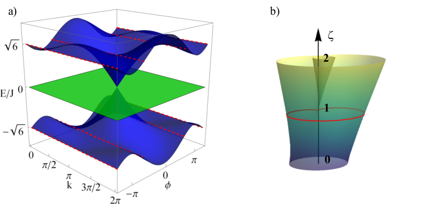
Figure 2: a) Spectrum of $\mathcal{H}(k,\phi_{1},\phi_{2})$ for $J_{i}=J$ with i $\in(1,2,t1,t2)$ and $\phi_{1}=\phi_{2}=\phi$. The red dashed lines show the $\phi$ values that give four flat bands. b) Cylindrical plot of the surface $\rho(\phi,\zeta)=1+\zeta\cos(\phi)$

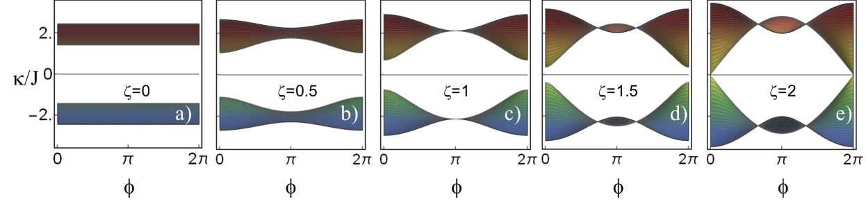
Figure 3: Spectrum support on the $(\kappa,\phi)$ plane for different values of $\zeta$.

III Aharonov-Bohm caging

A peculiarity of the two-flux model is that the caging arises due to the destructive interference of waves propagating along three arms. This implies that, at variance with the standard two-arm single-flux AB cagesLonghi (2014), the values of $\phi_{1}$ and $\phi_{2}$ where the caging effect appears can be controlled by changing the tunnel couplings J. We remark that when caging arises due to the destructive interference of waves propagating along two arms it has to be necessarily located at $\phi=\pi$, i.e. the total amplitude is given by the sum of two identical terms having opposite sign. On the contrary, as stated above, in the $\theta$-lattice we find different caging conditions depending on the tunnel couplings. In particular, when all J’s are equal, caging appears for $\phi_{1}=\phi_{2}=2\pi/3$ and $\phi_{1}=\phi_{2}=4\pi/3$ reflecting the trigonal symmetry of the unit cell. For arbitrary values of the $J$’s and $\phi_{1}=\phi_{2}=\phi$ the condition to have dispersionless bands can be written as follows

$$1+\zeta\cos(\phi)=0$$ (8)

where $\zeta=2J_{t2}J_{t1}/(J_{1}J_{2})$. In Fig.2b) we show a cylindrical plot of the surface $\rho(\phi,\zeta)=1+\zeta\cos(\phi)$, where we clearly distinguish three cases: for $\zeta>1$ we have two values of $\phi\in[0,2\pi\,[$ where Eq.(8) is satisfied, for $\zeta<1$ the caging condition is never fulfilled, while for $\zeta=1$ Eq.(8) admits only the solution $\phi=\pi$ as in the case of the standard two-arm AB caging.

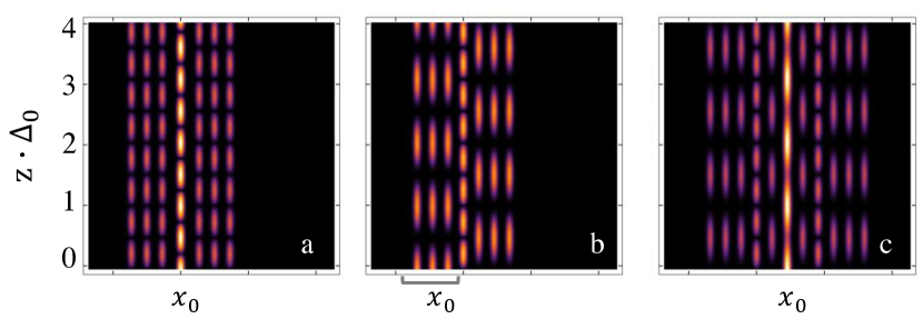
Figure 4: Light dynamics in the presence of AB caging for three different injection configurations: (a) $|\psi_{0}\rangle=|a_{n_{0}}\rangle$, (b) $|\psi_{0}\rangle=\frac{1}{\sqrt{3}}(|b_{n_{0}}\rangle+|c_{n_{0}}\rangle+|d_{n_{0}}\rangle)$ and (c) $|\psi_{0}\rangle=|c_{n_{0}}\rangle$. Lattice parameters: $J_{1}=J_{2}=J_{t1}=J_{t2}=J$, $\phi_{1}=\phi_{2}=\phi=2\pi/3$, $\Delta_{0}=\sqrt{6}J$, $N=40$, $n_{0}=20$.

To further analyze how caging arises when $\phi_{1}=\phi_{2}=\phi$, in Fig.3 (a-e) we show the evolution of the quasi-energy spectrum support as $\zeta$ increases from $\zeta=0$ to $\zeta=2$. At $\zeta=0$, corresponding to $J_{t1}J_{t2}=0$, the spectrum is clearly $\phi$-independent; as we increase $\zeta$ we find a pseudo-localization region around $\phi=\pi$ that evolves in a fully localized spectrum for $\zeta=1$; eventually for $\zeta>1$, the spectrum support shows two nodes, signaling the emergence of genus 2 AB caging.

Let us now consider the light dynamics in the different caging regimes. As discussed by several Authors, see e.g. Longhi (2014); Christodoulides, Lederer, and Silberberg (2003), assuming evanescent coupling of single-mode waveguides, it is described by the following coupled mode equations:

$$\left\{\begin{array}[]{rcl}i\partial_{z}a_{n}&=&J_{1}b_{n}+J_{2}b_{n-1}+J_{t1}(e^{i\phi_{1}}c_{n}+e^{-i\phi_{2}}d_{n})+\\ &&+J_{t2}(c_{n-1}+d_{n-1})\\[2.84544pt] i\partial_{z}b_{n}&=&J_{1}a_{n}+J_{2}a_{n+1}\\[2.84544pt] i\partial_{z}c_{n}&=&J_{t1}e^{-i\phi_{1}}a_{n}+J_{t2}a_{n+1}\\[2.84544pt] i\partial_{z}d_{n}&=&J_{t1}e^{i\phi_{2}}a_{n}+J_{t2}a_{n+1}\end{array}\right.$$ (9)

where $\partial_{z}$ indicate the partial derivative with respect to $z$. Solving numerically the above equations on a finite lattice with $N$ unit cells (4$N$ sites) and open boundary conditions yields the results shown in Figs. 4 and 5.

In Figure 4 we simulate the propagation of a light beam injected at $z=0$ in a $\theta$-lattice consisting of $N$ unit cells, $4N$ waveguides, with homogeneous tunnel couplings $J_{i}=J$ and fluxes $\phi_{1}=\phi_{2}=\phi=2\pi/3$. For these parameters the dispersive bands $\kappa_{\pm}$ become flat and, independently of the precise position and energy of the incoming beam, light gets trapped on a cluster of few waveguides. Only the structure of the caging cluster depends on the initial condition. This is due to the fact that, depending on the initial condition, different localized bands enter the dynamics. When the light is injected in a site $A$ only the upper and lower bands are dynamically occupied; caging then implies that only the waveguide $A_{n}$ and the six surrounding waveguides $b_{n},c_{n},d_{n}$ and $b_{n-1},c_{n-1},d_{n-1}$ are populated as shown in Fig.4a). The wavelength, $\lambda_{0}$, of the oscillations between the upper and lower bands is clearly given by the inverse of the spectral gap i.e. $\lambda_{0}=1/(2\Delta_{0})$ with $\Delta_{0}=\Delta(k,2\pi/3,2\pi/3)=\sqrt{6}J$. A somewhat similar situation arises when light is injected symmetrically in the waveguides $b_{n},c_{n},d_{n}$, i.e. creating the initial state $|\psi_{0}\rangle=\frac{1}{\sqrt{3}}(|b_{n_{0}}\rangle+|c_{n_{0}}\rangle+|d_{n_{0}}\rangle)$. The peculiar structure of the initial state implies that in this case, shown in Fig. 4(b), the light beam undergoes oscillations between the cell $n$ and $n+1$ along $z$ without modifying its shape. Eventually in Fig. 4(c) we show the propagation of a light beam injected from the site $c_{n}$. In this case the evolution involves also the degenerate bands and the signal spreads over three unit cells.

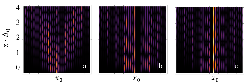
Figure 5: Dispersive light dynamics for $\phi_{1}=\phi_{2}=\phi=\pi$, i.e. away from the AB caging condition, for three different injection configurations: (a) $|\psi_{0}\rangle=|a_{n_{0}}\rangle$, (b) $|\psi_{0}\rangle=|b_{n_{0}}\rangle$ and (c) $|\psi_{0}\rangle=|c_{n_{0}}\rangle$. Other lattice parameters as in Fig. 4.

When the caging condition is not fulfilled, light spreads to the entire lattice. This situation is considered in Fig.5 where we set $\phi_{1}=\phi_{2}=\pi$ and the other parameters as in Fig. 4. These values of the fluxes are special under many respects: first, as discussed in the following section, they yield, Fig.5a), a weaker dispersion as compared e.g. to the case $\phi_{1}=\phi_{2}=0$, and second, they yield destructive Aharonov-Bohm interference on specific sites of the array. For example, as shown in Fig.5(b), for a "$b$" type injection waveguide, the propagation does not involve the sites "$c$" and "$d$" in the same plaquette, while, as shown in Fig.5(c), for a "$c$" type injection waveguide, the propagation does not involve the site "$b$" in the same plaquette. This is due to the fact that, at $\phi_{1}=\phi_{2}=\pi$ there are two tunneling paths from $b$ to $c$ and from $b$ to $d$ having opposite signs and equal amplitudes.

IV Signatures of Aharonov-Bohm interference in the diffraction patterns

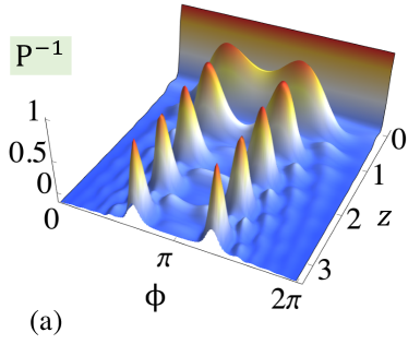
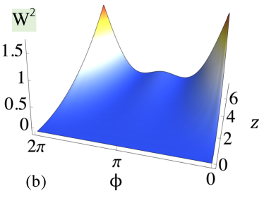
Figure 6: Inverse participation ratio (a) and average width (b) as functions of $z$ and $\phi$. Other lattice parameters as in Fig. 4

Beside inducing AB caging, synthetic gauge fields modulate light propagation in photonic lattices through AB interference, mimicking the action of their electromagnetic counterparts and yielding synthetic-flux dependent diffraction effects. Purpose of the present section is to highlight how these effects arise in the $\theta$-lattice. To characterize diffraction for different values of the synthetic fluxes we will focus on two quantities, namely, the inverse participation number, $P^{-1}$, defined as

$$P^{-1}=\sum_{x}|\Psi_{x}|^{4},$$ (10)

where $\Psi_{x}$ denotes the field’s amplitude at position $x=na$ along the lattice, with "a" the lattice period, and the average square width, $W^{2}$, defined as

$$W^{2}=\frac{\langle x^{2}\rangle-\langle x\rangle^{2}}{N^{2}}$$ (11)

with $\langle x^{\alpha}\rangle=\sum_{x}x^{\alpha}|\psi_{x}|^{2}$. The inverse participation number is always smaller or equal 1 and it gives a measure of the number of sites where photons are confined, specifically we have $P=1$ when light is confined to a single waveguide and $P\sim m$ when light is confined to a cluster of $m$ waveguides. The average width $W$ is useful to characterize how the signal disperse, it equals zero in the presence of caging and in standard photonic waveguide lattices it grows as $z^{2}$. In Figure 6(a) we plot the participation ratio as a function of $z$ and $\phi$ for a lattice with homogeneous tunnel couplings and fluxes, i.e. $\phi_{i}=\phi$ and $J_{i}=J_{ti}=J$ with $i=1,2$. We assume that the system is initially prepared in the fully localized state $|a_{n_{0}}\rangle$, at $z=0$ we thus have $P^{-1}=1$ independently of $\phi$. As $z$ increases, light start dispersing and we clearly see the emergence of two peaks at $\phi=2\pi/3$ and $\phi=4\pi/3$ due to AB caging. We also notice that $P^{-1}$ has a strongly oscillating behavior with $z$ that is associated with dynamic oscillations between different bands. The presence of these oscillations may hinder the characterization of the difference interference regimes by simply measuring the amplitude of the fields in a small cluster of sites for a given propagation length $z=\bar{z}$. For this purpose, the square width $W^{2}$ defined in Eq.(11) may be more appropriate as we show in Figure 6(b). There, we notice in particular the emergence of a smooth double-well structure associated with AB interference. Having a monotonic behavior as a function of $z$, $W$ can be used to characterize the different diffraction regimes for different values of the synthetic fluxes and $J$’s. This is what we do in Fig. 7 (a-b) to illustrate the tunability of the caging effect in the $\theta$-lattice. In Fig. 7 (a) we show a density plot of the width $W$ calculated at $zJ=10$ for the system initially prepared in the state $|a_{n_{0}}\rangle$, as a function of $\phi_{1}$ and $\phi_{2}$ for homogeneous tunnelings. We clearly see that the contour $W=0.5$ represented by the dashed black line essentially allows us to distinguish between a weakly dispersing region including the caging points $\phi_{1}=\phi_{2}=2\pi/3$ and $\phi_{1}=\phi_{2}=4\pi/3$ and a strongly dispersing region for $\phi\lesssim\pi/2$. In Fig. 7 (b) we plot $W_{z=10J}$ as a function of $\phi$ and $J_{t2}$ setting all other tunnel couplings to $J$. In this figure the black dashed line indicates the caging condition given by Eq. (8). We notice that when $J_{t2}$ becomes much larger than $J$ the tunability essentially disappears, this is due to the fact that increasing $J_{t2}$ corresponds to decrease the weight of interference paths going through the site $b$ bringing the lattice back to the single flux regime.

Figure 7: Density plot of the width $W$ as a function of $\phi_{1}$ and $\phi_{2}$ and as a function of $J_{t2}$ and $\phi=\phi_{1}=\phi_{2}$.

V Conclusions

We presented a theoretical study of transport of light in a strip of theta-shaped plaquettes subjected to synthetic magnetic fields. We showed how to realize Aharonov-Bohm cages that prevent the photon beam to escape from finite clusters. Suitably chosen fluxes with selected input configurations enables tuning the cage size. Our results have relevance for fundamental properties of topological lattice and various applications as in non-diffractive image transmission schemesVicencio et al. (2015); Xia et al. (2016), all-optical logic gatesReal et al. (2017) and optical data processing.

DATA AVAILABILITY

The data that support the findings of this study are available from the corresponding author upon reasonable request.