On the stickiness of CO₂ and H₂O ice particles

Abstract

Laboratory experiments revealed that CO₂ ice particles stick less efficiently than H₂O ice particles, and there is an order of magnitude difference in the threshold velocity for sticking. However, the surface energies and elastic moduli of CO₂ and H₂O ices are comparable, and the reason why CO₂ ice particles were poorly sticky compared to H₂O ice particles was unclear. Here we investigate the effects of viscoelastic dissipation on the threshold velocity for sticking of ice particles using the viscoelastic contact model derived by Krijt et al. We find that the threshold velocity for sticking of CO₂ ice particles reported in experimental studies is comparable to that predicted for perfectly elastic spheres. In contrast, the threshold velocity for sticking of H₂O ice particles is an order of magnitude higher than that predicted for perfectly elastic spheres. Therefore, we conclude that the large difference in stickiness between CO₂ and H₂O ice particles would mainly originate from the difference in the strength of viscoelastic dissipation, which is controlled by the viscoelastic relaxation time.

1 Introduction

Pairwise collisional growth of dust aggregates is the first step of planet formation (e.g., Johansen et al., 2014). The stickiness and collisional behavior of silicate dust particles/aggregates have been reported in a large number of studies (e.g., Poppe et al., 2000; Blum & Wurm, 2008; Seizinger et al., 2013; Kimura et al., 2015; Gunkelmann et al., 2016; Quadery et al., 2017; Planes et al., 2020). Particles/aggregates composed of H₂O ice are generally found to be stickier (e.g., Shimaki & Arakawa, 2012; Gundlach & Blum, 2015), although Kimura et al. (2020) claimed that H₂O ice particles might not be stickier than crystalline silicate particles. This difference in behavior plays an important role in models of dust evolution and planetesimal formation in the inner a few au of circumstellar disks (e.g., Drążkowska & Alibert, 2017).

In the cooler outer region of circumstellar disks, not only H₂O ice but also CO₂ and/or CO ices are important constituents of icy dust particles (e.g., Öberg & Bergin, 2020). The condensation temperatures of CO₂ and CO ices are approximately $70\ {\rm K}$ and $20\ {\rm K}$, respectively (see Okuzumi et al., 2016). Using the minimum mass solar nebula model (Hayashi, 1981), Musiolik et al. (2016a) found that the location of the CO₂ snow line is at $9.3\ {\rm au}$ from the Sun, which is close to the current orbit of Saturn. Ali-Dib et al. (2014) also suggests that Uranus and Neptune might be formed near the CO snow line based on the high atmospheric C/H and low N/H ratios. Therefore, CO₂ and CO ices may play a crucial role in the planet formation.

In addition, the stickiness of CO₂ ice particles is of great importance for understanding the dust growth and radial drift behavior in circumstellar disks (Pinilla et al., 2017). Recent (sub)millimeter polarimetric observations of circumstellar disks around young stars (e.g., Kataoka et al., 2017; Stephens et al., 2017) revealed the abundant presence of ${\sim}100\ \upmu{\rm m}$-sized dust particles beyond the H₂O snow line. In contrast, the classical theory for dust growth (e.g., Dominik & Tielens, 1997; Wada et al., 2009) suggests that H₂O ice particles can grow into significantly larger aggregates when turbulence in a circumstellar disk is moderate. To solve this discrepancy, Okuzumi & Tazaki (2019) proposed an idea that the low stickiness of CO₂ ice particles reported by Musiolik et al. (2016a, b) might be the key to explain the small size of dust particles observed in circumstellar disks.

Laboratory experiments by Musiolik et al. (2016a, b) revealed that CO₂ ice particles are less sticky compared to H₂O ice particles. Pinilla et al. (2017) and Okuzumi & Tazaki (2019) proposed that the large difference in stickiness between H₂O and CO₂ ice particles would originate from the difference in the dipole moment. In other words, the low threshold velocity for sticking of CO₂ ice particles is due to the small surface free energy of apolar CO₂ ice. However, we note that the literature value of the surface free energy of CO₂ ice ($80\ {\rm mJ}\ {\rm m}^{-2}$; Wood, 1999) is comparable to that of H₂O ice ($100\ {\rm mJ}\ {\rm m}^{-2}$; Israelachvili, 2011). In addition, the values of elastic properties (i.e., the Young’s modulus and Poisson ratio) are also similar between two materials (see Section 3). In the framework of Dominik & Tielens (1997), one would then expect the threshold velocity for sticking to be similar for H₂O and CO₂ ices.

In this study, we investigate another possibility to explain the low threshold velocity for sticking of CO₂ ice particles compared to that of H₂O ice particles. Krijt et al. (2013) constructed a viscoelastic contact model, which is the advanced version of the contact theory for perfectly elastic spheres (e.g., Johnson et al., 1971; Wada et al., 2007). The viscoelastic contact model of Krijt et al. (2013) takes into account a crack propagation at the edge of the contact and an energy dissipation arising from viscoelastic behavior beneath the contact. Applying this model to water ice particles, Gundlach & Blum (2015) found that the threshold velocity for sticking is up to an order of magnitude higher than that predicted from the theory for perfectly elastic spheres. Therefore, we can potentially explain the large difference in stickiness between H₂O and CO₂ ice particles reported by Musiolik et al. (2016a, b) if CO₂ ice particles follow more closely the contact theory for perfectly elastic adhesive spheres.

The structure of this paper is as follows. In Section 2, we review the viscoelastic contact model derived by Krijt et al. (2013). In Section 3, we summarize the material properties of CO₂ ice. In Section 4, we show the typical results for collisions between two viscoelastic spheres. In Section 5, we calculate the threshold velocity for sticking and compare our numerical results with experimental data reported by Musiolik et al. (2016a, b). In Section 6, we evaluate the critical velocity for collisional growth/fragmentation of dust aggregates. Implications of our results are discussed in Section 7, and we conclude in Section 8.

2 Contact Model

The contact model used in this study is identical to what Krijt et al. (2013) derived. In Section 2, we briefly summarize their viscoelastic contact model.

2.1 Elastic strain energy stored in a contact

When two elastic spheres are pressed together, they will deform locally and share a circular contact area with radius, $a$. The pressure distribution in the contact area, $p{\left(r\right)}$, is given as a function of the distance from the center of the contact, $r$, as follows (Muller et al., 1980):

$$p{\left(r\right)}=\frac{E^{*}}{\pi R}\frac{a^{2}-2r^{2}+R\delta}{\sqrt{a^{2}-r^{2}}},$$ (1)

where $\delta$ is the mutual approach, $R$ is the reduced particle radius, and $E^{*}$ is the elastic contact modulus. For a contact between two spheres with the same radius and material, $R$ and $E^{*}$ are given by $R=R_{1}/2$ and $E^{*}=E/{\left[2{\left(1-\nu^{2}\right)}\right]}$, where $R_{1}$ is the particle radius, $E$ is the (relaxed) Young’s modulus, and $\nu$ is the Poisson ratio. Then the elastic strain energy stored in the contact, $U_{\rm E}$, is given by (Muller et al., 1980)

$$U_{\rm E} = \frac{1}{2}\int_{0}^{a}{\rm d}r\ 2\pi r{p{\left(r\right)}}{w{\left(r\right)}}$$ (2)

$$= \frac{E^{*}a^{3}}{3R}{\left[\delta{\left(\frac{3\delta R}{a^{2}}-1\right)}-\frac{a^{2}}{5R}{\left(\frac{5\delta R}{a^{2}}-3\right)}\right]},$$

where $w{\left(r\right)}=\delta-{r^{2}}/{\left(2R\right)}$ is the deformation of the surface of spheres.

2.2 Johnson–Kendall–Roberts theory

Johnson et al. (1971) introduced a surface energy term, $U_{\rm S}$, to describe a contact between adhesive particles:

$$U_{\rm S}=-\pi a^{2}\gamma.$$ (3)

Assuming that the contact area changes quasistatically, ${\partial U_{\rm S}}/{\partial a}$ is given by

$$\frac{\partial U_{\rm S}}{\partial a}=-2\pi a\gamma.$$ (4)

It is known that an equilibrium exists in the framework of Johnson–Kendall–Roberts theory (hereinafter referred to as JKR theory; Johnson et al., 1971). If there are no external forces, the contact radius at the equilibrium is

$$a_{\rm eq}={\left(\frac{9\pi\gamma R^{2}}{2E^{*}}\right)}^{1/3},$$ (5)

and the mutual approach at the equilibrium is given by

$$\delta_{\rm eq} = \frac{{a_{\rm eq}}^{2}}{R}-\sqrt{\frac{2\pi\gamma a_{\rm eq}}{E^{*}}}$$ (6)

$$= {\left(\frac{3\pi^{2}R\gamma^{2}}{4{E^{*}}^{2}}\right)}^{1/3}.$$

Johnson et al. (1971) assumed that there are no forces acting outside the contact area for simplicity. This treatment works well when the Tabor parameter, $\mu$, is sufficiently large, i.e., $\mu\gg 1$ (Tabor, 1977). The Tabor parameter is defined as

$$\mu=\frac{1}{\epsilon}{\left(\frac{R\gamma^{2}}{{E^{*}}^{2}}\right)}^{1/3},$$ (7)

where $\epsilon$ is the range of action of the surface forces and $\gamma$ is the surface energy. We set $\epsilon=0.3\ {\rm nm}$ in this study (Krijt et al., 2013). Using material properties of CO₂ ice, we found that $\mu\simeq 9.5$ for $R_{1}=60\ \upmu{\rm m}$, and JKR theory could be appliable for (sub)micron-sized CO₂ ice particles.

2.3 Viscoelastic crack velocity

If spheres are made of perfectly elastic materials, we can use the surface energy term introduced by Johnson et al. (1971). However, when the material is viscoelastic, the propagating cracks have non-zero velocities and we can no longer use Equation (4) to calculate the surface energy term. In this case, the energy released/absorbed when the crack is closed/opened, ${\partial U_{\rm S}^{*}}/{\partial a}$, is

$$\frac{\partial U_{\rm S}^{*}}{\partial a}=-2\pi aG_{\rm eff},$$ (8)

where $G_{\rm eff}$ is the apparent surface energy for bonding/cracking. The apparent surface energy, $G_{\rm eff}$, depends on the crack velocity, $\dot{a}$. Here we introduce the normalized apparent surface energy, $\beta$, and the normalized crack velocity, $v$:

$$\beta \equiv \frac{G_{\rm eff}}{\gamma},$$ (9)

$$v \equiv \frac{{\sigma_{0}}^{2}T_{\rm vis}}{E^{*}\gamma}\dot{a},$$ (10)

where $\sigma_{0}=\gamma/\epsilon$ is the attractive force acting across the crack and $T_{\rm vis}$ is the viscoelastic relaxation time (Greenwood, 2004; Krijt et al., 2013). The normalized apparent surface energy, $\beta$, is a function of $k$ and $v$:

$$\beta=\beta{\left(k,v\right)},$$ (11)

where $k$ is the ratio of relaxed to instantaneous elastic moduli. In practice, $k\ll 1$ and we set $k=0.01$ as a fiducial value (Greenwood, 2004). We note that Krijt et al. (2013) set $k=0.02$ instead; however, this small difference in $k$ hardly changes our numerical results (see Figure 3). The normalized crack velocity is also a function of $k$ and $\beta$:

$$v=v{\left(k,\beta\right)}.$$ (12)

Figure 7 shows the dependence of $v$ on $\beta$ for different values of $k$ (see Greenwood, 2004). We describe how did we calculate $v{\left(k,\beta\right)}$ in Appendix A.

2.4 Apparent surface energy in equilibrium

Krijt et al. (2013) assumed that the crack velocity, $\dot{a}$, and the apparent surface energy, $G_{\rm eff}$, adjust themselves to satisfy the equilibrium contact condition:

$$\frac{\partial}{\partial a}{\left(U_{\rm E}+U_{\rm S}^{*}\right)}=0,$$ (13)

which can be solved to give

$$G_{\rm eff}=\frac{E^{*}}{2\pi aR^{2}}{\left(a^{2}-\delta R\right)}^{2}.$$ (14)

Then the apparent surface energy, $G_{\rm eff}=G_{\rm eff}{\left(a,\delta\right)}$, is given by Equation (14) and the crack velocity, $\dot{a}=\dot{a}{\left(a,\delta\right)}$, is given by Equation (12).

2.5 Elastic and dissipative forces

The pressure distribution in the contact area is given by Equation (1), and the integral over the contact area yields the elastic force between two particles, $F_{\rm E}$:

$$F_{\rm E} = \int_{0}^{a}{\rm d}r\ 2\pi r{p{\left(r\right)}}$$ (15)

$$= \frac{2E^{*}}{3R}{\left(3a\delta R-a^{3}\right)}.$$

When two viscoelastic particles collide and deform, a significant amount of energy could be dissipated. Following Krijt et al. (2013), we write the dissipative force as follows:

$$F_{\rm D} = \int_{0}^{a}{\rm d}r\ 2\pi rA\frac{\partial{p{\left(r\right)}}}{\partial\delta}\dot{\delta}$$ (16)

$$= 2AE^{*}a\dot{\delta},$$

where $A=T_{\rm vis}/\nu^{2}$ (Brilliantov et al., 1996, 2007). The dissipative force, $F_{\rm D}$, depends on $a$ and $\dot{\delta}$, and it acts as a drag term.

For a head-on collision of identical spheres, the time evolution of the mutual approach is given by

$$\ddot{\delta}=-\frac{1}{m^{*}}{\left(F_{\rm E}+F_{\rm D}\right)},$$ (17)

where $m^{*}$ is the reduced mass, which is $m^{*}=m_{1}/2$ for a contact between two spheres with the same radius and material. The mass of each particle is given by $m_{1}=4\pi\rho{R_{1}}^{3}/3$, where $\rho=1560\ {\rm kg}\ {\rm m}^{-3}$ is the material density of CO₂ ice (Mazzoldi et al., 2008).

Ignoring long-range forces, the moment of first contact is taken as $t=0$, and the initial condition for the mutual approach is $\delta=0$ and $\dot{\delta}=V_{\rm in}$, where $V_{\rm in}$ is the collision velocity. The normalized crack velocity, $v=v{\left(k,\beta\right)}$, is defined within the range of $k<\beta<1/k$ (see Appendix A) and the apparent surface energy satisfies $G_{\rm eff}=\beta\gamma>0$. Equation (14) is rewritten as $G_{\rm eff}=E^{*}a^{3}/{\left(2\pi R^{2}\right)}$ when $\delta=0$, and it does not allow $a=0$ as the initial condition. For our numerical integrations, we set $\beta={\left(1+\varepsilon\right)}k$ at $t=0$ as Krijt et al. (2013) assumed. We use the small value of $\varepsilon=0.01$. We end integrations when $\beta={\left(1-\varepsilon\right)}/k$, and two spheres will separate immediately. These assumptions are justified as the contact evolves rapidly near $a\simeq 0$ and $\delta$ hardly changes (see Appendix B of Krijt et al., 2013).

3 Material Properties of Carbon Dioxide Ice

In Section 3, we discuss the elastic and adhesive material properties of CO₂ and H₂O ices, needed for solving Equation (17). Following Gundlach & Blum (2015), we treat the main viscoelastic parameter $T_{\rm vis}$ as a free parameter that may depend on particle size.

3.1 Surface free energy

The surface free energies of crystals are proportional to their sublimation energies (e.g., Shuttleworth, 1949; Benson & Claxton, 1964). Using the crystal structure and the latent heat of sublimation of CO₂ ice, Wood (1999) theoretically estimated the surface free energy of CO₂ ice as $\gamma_{\rm SV}=80\ {\rm mJ}\ {\rm m}^{-2}$. This value is widely used in the studies of CO₂ clouds in the martian atmosphere (e.g., Määttänen et al., 2005; Nachbar et al., 2016; Mangan et al., 2017). Glandorf et al. (2002) also obtained an approximate value of $\gamma_{\rm SV}$ by using the Antonoff’s rule, and the surface free energy is estimated as $67\ {\rm mJ}\ {\rm m}^{-2}$, which is in reasonable agreement with that obtained by Wood (1999).

For a contact between two spheres made of same material, the surface energy, $\gamma$, is (approximately) twice the surface free energy (Johnson et al., 1971):

$$\gamma=2\gamma_{\rm SV}.$$ (18)

For H₂O ice, the canonical value of $\gamma_{\rm SV}$ is $\gamma_{\rm SV}=100\ {\rm mJ}\ {\rm m}^{-2}$ (Israelachvili, 2011). We note, however, that the surface free energy of H₂O ice is still under debate (see Section 5.2).

3.2 Young’s modulus and Poisson ratio

As the longitudinal and transversal velocities of sound, $v_{\rm lg}$ and $v_{\rm ts}$, are related to the elastic properties, we can calculate the Young’s modulus and Poisson ratio from the results of sound velocity measurements. These sound velocities, $v_{\rm lg}$ and $v_{\rm ts}$, are given by (e.g., Han & Batzle, 2004)

$$v_{\rm lg} = \sqrt{\frac{1}{\rho}{\left(\mathcal{K}+\frac{4}{3}\mathcal{G}\right)}},$$ (19)

$$v_{\rm ts} = \sqrt{\frac{\mathcal{G}}{\rho}},$$ (20)

where $\mathcal{K}$ is the bulk modulus and $\mathcal{G}$ is the shear modulus. Both $\mathcal{K}$ and $\mathcal{G}$ can be rewritten by using $E$ and $\nu$ as follows:

$$\mathcal{K} = \frac{E}{3{\left(1-2\nu\right)}},$$ (21)

$$\mathcal{G} = \frac{E}{2{\left(1+\nu\right)}}.$$ (22)

Yamashita & Kato (1997) measured the longitudinal and transversal velocities of sound in CO₂ ice and obtained $v_{\rm lg}=2900\ {\rm m}\ {\rm s}^{-1}$ and $v_{\rm ts}=1650\ {\rm m}\ {\rm s}^{-1}$ at the temperature of $80\ {\rm K}$ (see Musiolik et al., 2016a). Then the Young’s modulus and Poisson ratio are $E=10.7\ {\rm GPa}$ and $\nu=0.26$, respectively.

For H₂O ice, the literature values of $E=7\ {\rm GPa}$ and $\nu=0.25$ are widely used in previous studies (e.g., Dominik & Tielens, 1997; Wada et al., 2007; Gundlach & Blum, 2015).

4 Sticking, Bouncing, and Double Collisions

The contact model reviewed in Section 2 can be used to calculate the time evolution of the contact between two colliding spheres. In Section 4, we show the typical results for collisions between two equal-sized spheres of CO₂ ice.

We begin by setting $R_{1}=60\ \upmu{\rm m}$ and $T_{\rm vis}=10^{-9}\ {\rm s}$, and exploring a range of impact collision velocities $V_{\rm in}$. We found that there are three types of collision outcomes, namely, sticking collisions, bouncing collisions, and double collisions. Similar results are also reported in Sections 3.1 and 3.2 of Krijt et al. (2013).

4.1 Sticking collision

The grey lines of Figure 1 show the evolution of the contact radius, $a$, the mutual approach, $\delta$, and the approaching velocity, $\dot{\delta}$, for a head-on collision at $V_{\rm in}=3.5\ {\rm cm}\ {\rm s}^{-1}$. The green stars mark the equilibrium point in JKR theory ($a=a_{\rm eq}$, $\delta=\delta_{\rm eq}$, and $\dot{\delta}=0$). At the start of the collision, $t=0$, the mutual approach is $\delta=0$ and the contact radius is given by

$$a={\left[\frac{2\pi R^{2}}{E^{*}}{\left(1+\varepsilon\right)}k\gamma\right]}^{1/3}.$$ (23)

The contact radius initially grows very rapidly, as $a$ increases to $a\simeq 0.3\ \upmu{\rm m}$ with $\delta$ hardly changing. Krijt et al. (2013) described the details of the behavior of the viscoelastic contact, by comparing with that of JKR theory (e.g., Wada et al., 2007).

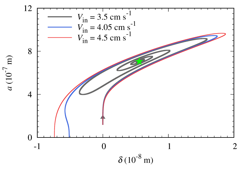
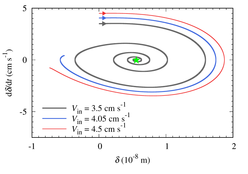
Figure 1: Time evolution of the contact radius, $a$, the mutual approach, $\delta$, and the approaching velocity, $\dot{\delta}$, for head-on collisions. The green stars mark the equilibrium point in JKR theory ($a=a_{\rm eq}$, $\delta=\delta_{\rm eq}$, and $\dot{\delta}=0$). The left panel shows the evolution in $\delta$–$a$ plane, and the right panel is the evolution in $\delta$–$\dot{\delta}$ plane, respectively. The grey lines represent the evolutionary track for the case of $V_{\rm in}=3.5\ {\rm cm}\ {\rm s}^{-1}$, resulting in sticking. The blue lines are for the case of $V_{\rm in}=4.05\ {\rm cm}\ {\rm s}^{-1}$, resulting in double collision in the collisional sequence. The red lines are for the case of $V_{\rm in}=4.5\ {\rm cm}\ {\rm s}^{-1}$, resulting in bouncing.

The most important difference between our viscoelastic contact model and JKR theory is whether the kinetic energy dissipates during contact or not. For the case of $V_{\rm in}=3.5\ {\rm cm}\ {\rm s}^{-1}$, the spheres cannot separate and instead oscillate back and forth. In $\delta$–$a$ and $\delta$–$\dot{\delta}$ planes, the contact spirals toward the equilibrium point of JKR theory due to the dissipative effects when we use the viscoelastic contact model. In the framework of JKR theory, in contrast, the oscillation would not be dampened. The dissipative effects increase the threshold velocity for sticking, $V_{\rm stick}$ (see Section 5).

4.2 Bouncing collision

Even if the dissipative effects work, collisions of two spheres will result in bouncing as the collision velocity is increased. The red lines of Figure 1 show the evolution of $a$, $\delta$, and $\dot{\delta}$, for a head-on collision at $V_{\rm in}=4.5\ {\rm cm}\ {\rm s}^{-1}$. In this case, the contact radius finally becomes $a\simeq 0$, and the mutual approach and the approaching velocity are $\delta>0$ and $\dot{\delta}<0$ at the end of the contact. At that point, the spheres separate and move away from each other at a velocity $V_{\mathrm{out}}$ (see Section 4.4).

4.3 Double collision

There exists a narrow range of impact velocities for which we observe a “double collision”. This double collision occurs as a result of energy dissipations and viscoelastic cracking. The blue lines of Figure 1 show the evolution of $a$, $\delta$, and $\dot{\delta}$, for a head-on collision at $V_{\rm in}=4.05\ {\rm cm}\ {\rm s}^{-1}$. In this case, the mutual approach and approaching velocity are $\delta>0$ and $\dot{\delta}>0$ at the end of the contact. As $\dot{\delta}>0$, two spheres are expected to recollide after their separation. We therefore named this outcome as the “double collision”. We note that the collision velocity of the second collision is much lower than that of the first collision because of dissipative effects, and the second collision should result in sticking.

4.4 Coefficient of restitution

We use the coefficient of restitution, $e$, to describe colllision outcomes. The definition of $e$ is

$$e\equiv-\frac{V_{\rm out}}{V_{\rm in}},$$ (24)

where $V_{\rm out}$ is the approaching velocity at the end of the contact. We set $e=0$ for sticking collisions. For double collisions, negative values of the coefficient of restitution will be obtained from numerical calculations. We note, however, that the second collision may occur immediately after the first collision and the final outcome of the collisional sequence is sticking. Then we can imagine that the “observed” value of the coefficient of restitution in laboratory experiments is $e=0$ for double collisions.

Figure 2 shows the variations of $e$ with $V_{\rm in}$ for $R_{1}=60\ \upmu{\rm m}$ and $T_{\rm vis}=10^{-9}\ {\rm s}$, a transition from sticking collisions to double collisions occurs at $V_{\rm in}=4.04\ {\rm cm}\ {\rm s}^{-1}$, and a transition from double collisions to bouncing collisions occurs at $V_{\rm in}=4.14\ {\rm cm}\ {\rm s}^{-1}$. In this case, we obtain the threshold velocity for sticking as $V_{\rm stick}=4.14\ {\rm cm}\ {\rm s}^{-1}$. As $V_{\rm stick}$ depends on the particle radius and material properties including $\gamma_{\rm SV}$ and $T_{\rm vis}$, we can estimate the relaxation time of viscoelastic particles from literature values of $V_{\rm stick}$ which are experimentally determined (e.g., Krijt et al., 2013; Gundlach & Blum, 2015).

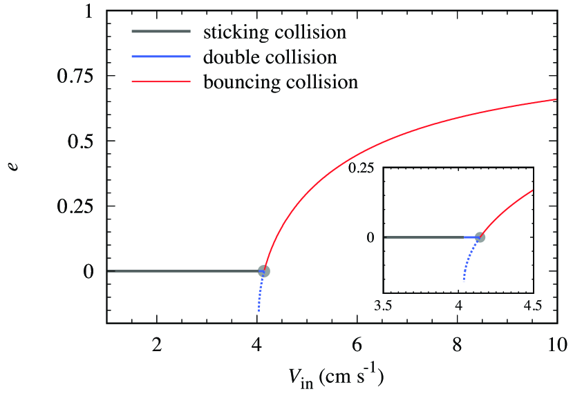
Figure 2: Variations of the coefficient of restitution, $e$, with the collision velocity, $V_{\rm in}$, for head-on collisions of CO₂ ice particles. Particle radius of $R_{1}=60\ \upmu{\rm m}$ and a relaxation time of $T_{\rm vis}=10^{-9}\ {\rm s}$ are assumed here. The grey, blue, and red solid lines represent the values of $e$ which are expected to be observed as final outcomes, and the blue dashed line is the value of $e$ obtained from numerical calculations (for double collisions). The grey point indicates the threshold velocity for sticking, $V_{\rm stick}=4.14\ {\rm cm}\ {\rm s}^{-1}$.

5 Threshold Velocity for Sticking

In section 5, we calculate the threshold velocity for sticking using the viscoelastic contact model, and we also compare our numerical results with experimental data reported by Musiolik et al. (2016a, b). We show that $V_{\rm stick}$ of both CO₂ and H₂O ice particles observed in experiments are consistent with the theoretical prediction from the viscoelastic contact model. Especially, $V_{\rm stick}$ of H₂O ice particles can be reproduced only when we consider the dissipative effects.

5.1 Carbon dioxide ice

Musiolik et al. (2016a) performed laboratory experiments of collisions of CO₂ ice particles within a vacuum chamber at a temperature of $80\ {\rm K}$. The collision velocities are below $2.5\ {\rm m}\ {\rm s}^{-1}$, and the typical radius of the particles is $R_{1}=60\ \upmu{\rm m}$ when we focus on the collisions of small particles whose radii are less than $150\ \upmu{\rm m}$. They found that the threshold velocity for sticking is $V_{\rm stick}={\left(0.04\pm 0.02\right)}\ {\rm m}\ {\rm s}^{-1}$, although the uncertainty is large.

Figure 3 shows the dependence of $V_{\rm stick}$ on $T_{\rm vis}$ for different values of $k$. As mentioned in Greenwood (2004) and Krijt et al. (2013), the evolution of contact radius is almost independent of $k$ except for the start and end of the contact. Then the collision outcomes hardly depend on the choice of $k$ as long as we set $k\ll 1$ (see Appendix A).

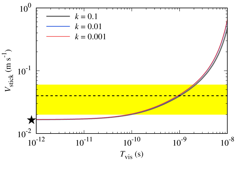
Figure 3: Dependence of the threshold velocity for sticking, $V_{\rm stick}$, on the relaxation time, $T_{\rm vis}$, for different values of $k$. The black dashed line represents the threshold velocity for sticking obtained from laboratory experiments and the yellow shaded region shows the uncertainty: $V_{\rm stick}={\left(0.04\pm 0.02\right)}\ {\rm m}\ {\rm s}^{-1}$ (see Musiolik et al., 2016a). The black star indicates the threshold velocity for sticking inferred from JKR theory, $V_{\rm stick,\,JKR}$ (e.g., Thornton & Ning, 1998; Wada et al., 2007). The typical radius of CO₂ ice particles used in Musiolik et al. (2016a) is $R_{1}=60\ \upmu{\rm m}$.

As shown in Figure 3, $V_{\rm stick}$ hardly changes when $T_{\rm vis}\lesssim 10^{-11}\ {\rm s}$. In this case, $V_{\rm stick}$ is almost identical to that of JKR theory. According to Thornton & Ning (1998), in the framework of JKR theory, the threshold velocity for sticking is given by

$$V_{\rm stick,\,JKR} = {\left(\frac{14.18}{m^{*}}\right)}^{1/2}{\left(\frac{\gamma^{5}R^{4}}{{E^{*}}^{2}}\right)}^{1/6}$$ (25)

$$= 1.66\times 10^{-2}\ {\left(\frac{R_{1}}{60\ \upmu{\rm m}}\right)}^{-5/6}\ {\rm m}\ {\rm s}^{-1}.$$

The black star plotted in Figure 3 indicates the value of $V_{\rm stick,\,JKR}$, and it is clear that $V_{\rm stick}\to V_{\rm stick,\,JKR}$ for the short-$T_{\rm vis}$ limit, $T_{\rm vis}\to 0$.

In contrast, when $T_{\rm vis}\gtrsim 10^{-9}\ {\rm s}$, the threshold velocity for sticking is several times higher than that predicted from JKR theory. The increase of $V_{\rm stick}$ with increasing of $T_{\rm vis}$ is also reported in previous studies (Krijt et al., 2013; Gundlach & Blum, 2015), and our results shown in Figure 3 are consistent with their results. Assuming that $k=0.01$, we can obtain the suitable range of $T_{\rm vis}$ to reproduce $V_{\rm stick}$ reported by Musiolik et al. (2016a) as follows:

$$8.5\times 10^{-11}\ {\rm s}\leq T_{\rm vis}\leq 1.97\times 10^{-9}\ {\rm s};$$ (26)

though we do not reject the possibility that $T_{\rm vis}\ll 10^{-10}\ {\rm s}$ and $V_{\rm stick}$ is nearly identical to $V_{\rm stick,\,JKR}$.

In numerical calculations, we assumed that CO₂ ice particles are spherical and the viscoelastic contact theory for spheres is appliable. We acknowledge, however, that CO₂ ice particles used in Musiolik et al. (2016a) are not spherical. Although Blum & Wurm (2000) suggested that irregular grains are slightly stickier than spherical grains, Musiolik et al. (2016a) mentioned that the effect of the irregular shape may be negligible.

Musiolik et al. (2016a, b) did not report the surface roughness of ice grains, however, it might alter the threshold velocity for sticking (e.g., Nagaashi et al., 2018). Although our results for both CO₂ and H₂O ice particles are consistent with the cases for smooth particles (see Sections 5.2 and 5.3), we need to assess the effect of the surface roughness in future.

It should also be noted that whether CO₂ ice particles were monolithic grains or aggregates is unknown. In this study, however, we assume that CO₂ ice particles whose radii are $R_{1}\simeq 60\ \upmu{\rm m}$ are monolithic. This is because the critical velocity for collisional growth/fragmentation, $V_{\rm frag}$, should be several times higher than $0.04\ {\rm m}\ {\rm s}^{-1}$ when CO₂ ice particles are aggregates, even if the monomer grains of these aggregates behaved as perfectly elastic spheres (see Section 7.1 for details).

5.2 Water ice

Musiolik et al. (2016b) also performed laboratory experiments of collisions of pure H₂O ice particles (and mixtured ice particles of H₂O–CO₂) within a vacuum chamber at a temperature of $80\ {\rm K}$. The typical radius of the particles is $R_{1}=90\ \upmu{\rm m}$, and their experimental results suggest that $V_{\rm stick}\sim 0.73\ {\rm m}\ {\rm s}^{-1}$ for pure H₂O ice particles.

Material properties of H₂O ice are reported in a large number of previous studies. We set $E=7\ {\rm GPa}$, $\nu=0.25$, and $\rho=930\ {\rm kg}\ {\rm m}^{-3}$ (Gundlach & Blum, 2015). The surface free energy of H₂O ice is still under debate. The canonical value of $\gamma_{\rm SV}$ used in numerical simulations (e.g., Wada et al., 2013; Sirono & Ueno, 2017; Tatsuuma et al., 2019) is $\gamma_{\rm SV}=100\ {\rm mJ}\ {\rm m}^{-2}$ (Israelachvili, 2011). Measurements of the critical rolling friction force of $\upmu{\rm m}$-sized H₂O ice particles suggest that $\gamma_{\rm SV}=190\ {\rm mJ}\ {\rm m}^{-2}$ (Gundlach et al., 2011), although the value of $\gamma_{\rm SV}$ depends on the assumed value of the critical rolling displacement (see Krijt et al., 2014). Moreover, tensile strength measurements in a low-temperature environment (Gundlach et al., 2018) suggest that $\gamma_{\rm SV}=20\ {\rm mJ}\ {\rm m}^{-2}$ at low temperatures below $150\ {\rm K}$. Musiolik & Wurm (2019) also reported that $\gamma_{\rm SV}$ at $175\ {\rm K}$ is one to two orders of magnitude lower than the canonical value based on their pull-off measurements of mm-sized water ice grains. Then we parameterize $\gamma_{\rm SV}$ in our calculations.

Figure 4 then shows the dependence of $V_{\rm stick}$ on $T_{\rm vis}$ for different values of $\gamma_{\rm SV}$. We found that we cannot explain the reported value of $V_{\rm stick}$ by using JKR theory, that is, the contact model for perfectly elastic adhesive spheres. Assuming that the range of the surface free energy is $20\ {\rm mJ}\ {\rm m}^{-2}\leq\gamma_{\rm SV}\leq 190\ {\rm mJ}\ {\rm m}^{-2}$, the required value of $T_{\rm vis}$ is

$$5.3\times 10^{-9}\ {\rm s}\leq T_{\rm vis}\leq 2.37\times 10^{-8}\ {\rm s},$$ (27)

and $T_{\rm vis}$ of H₂O ice particles with $R_{1}=90\ \upmu{\rm m}$ may be an order of magnitude larger than that of CO₂ ice particles with $R_{1}=60\ \upmu{\rm m}$.

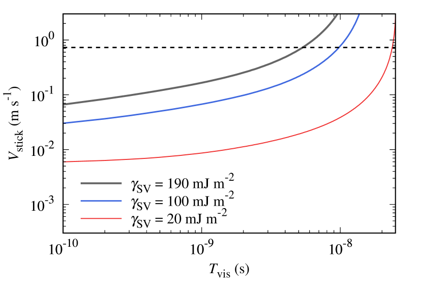
Figure 4: Dependence of the threshold velocity for sticking, $V_{\rm stick}$, on the relaxation time, $T_{\rm vis}$, for different values of $\gamma_{\rm SV}$. The black dashed line represents the threshold velocity for sticking obtained from laboratory experiments. The typical radius of H₂O ice particles used in Musiolik et al. (2016b) is $R_{1}=90\ \upmu{\rm m}$.

For H₂O ice particles with $R_{1}=1.5\ \upmu{\rm m}$, Gundlach & Blum (2015) revealed that $T_{\rm vis}=1\times 10^{-10}\ {\rm s}$ is plausible to reproduce the value of $V_{\rm stick}={\left(9.6\pm 0.3\right)}\ {\rm m}\ {\rm s}^{-1}$ obtained from their experiments. In Section 5.3, we discuss the dependence of $T_{\rm vis}$ on $R_{1}$.

5.3 Relaxation time

The relaxation time is a fitted parameter in this study because we do not know how $T_{\rm vis}$ relates to other fundamental material properties. We note, however, that there is an empirical relation between $T_{\rm vis}$ and $R_{1}$ (Krijt et al., 2013; Gundlach & Blum, 2015). Gundlach & Blum (2015) reported that the relaxation times obtained by Krijt et al. (2013) is consistent with a relation between $T_{\rm vis}$ and $R_{1}$, that is, $T_{\rm vis}\propto{R_{1}}^{1.11}$.

For H₂O ice particles with $R_{1}=1.5\ \upmu{\rm m}$, Gundlach & Blum (2015) revealed that $T_{\rm vis}=1\times 10^{-10}\ {\rm s}$. Therefore, the size-dependent relaxation time of H₂O ice particles may be given by (Gundlach & Blum, 2015)

$$T_{\rm vis,\,H_{2}O}=1\times 10^{-10}\ {\left(\frac{R_{1}}{1.5\ \upmu{\rm m}}\right)}^{1.11}\ {\rm s},$$ (28)

and this equation yields $T_{\rm vis,\,H_{2}O}=9.4\times 10^{-9}\ {\rm s}$ for H₂O ice particles with $R_{1}=90\ \upmu{\rm m}$. This relation shows excellent agreement with our numerical results (see Relation 27).

Then we also apply the empirical relation to the size-dependent relaxation time of CO₂ ice particles. From Relation (26), we found that the following relation,

$$T_{\rm vis,\,CO_{2}}=1\times 10^{-11}\ {\left(\frac{R_{1}}{1\ \upmu{\rm m}}\right)}^{1.11}\ {\rm s},$$ (29)

is consistent with the experimental results for CO₂ ice particles with $R_{1}=60\ \upmu{\rm m}$. Figure 5 shows the dependence of $T_{\rm vis}$ on $R_{1}$ for both CO₂ and H₂O ice particles.

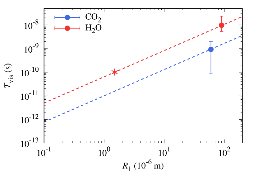
Figure 5: Dependence of the relaxation time, $T_{\rm vis}$, on the particle radius, $R_{1}$, for both CO₂ and H₂O ice particles. The blue and red points with error bars are the calculated values of $T_{\rm vis}$ for CO₂ and H₂O ice particles in this study, respectively. The red star shows a reported value of $T_{\rm vis,\,H_{2}O}$ from numerical calculations by Gundlach & Blum (2015). The dashed lines are the (empirical) fitting formulae of size-dependent $T_{\rm vis,\,CO_{2}}$ and $T_{\rm vis,\,H_{2}O}$.

5.4 Size dependence of threshold velocity for sticking

Here we calculate $V_{\rm stick}$ for (sub)$\upmu{\rm m}$-sized CO₂ ice particles by using the size-dependent relaxation time derived in Section 5.3. We set $\gamma_{\rm SV}=80\ {\rm mJ}\ {\rm m}^{-2}$, $E=10.7\ {\rm GPa}$, $\nu=0.26$, and $\rho=1650\ {\rm kg}\ {\rm m}^{-3}$ (see Section 3).

The left panel of Figure 6 shows $V_{\rm stick}$ as a functin of $R_{1}$. We also consider the dependence of $T_{\rm vis}$ on $V_{\rm stick}$. The grey line represents the case of perfectly elastic contact model, i.e., $V_{\rm stick}=V_{\rm stick,\,JKR}$. The blue line represents the standard model, i.e., $T_{\rm vis}=T_{\rm vis,\,CO_{2}}$ (Equation 29). We can find that the difference between these two models is within a factor of a few in $V_{\rm stick}$, and we can (roughly) evaluate $V_{\rm stick}$ by using JKR theory, which is widely used in previous studies (e.g., Dominik & Tielens, 1997; Wada et al., 2007).

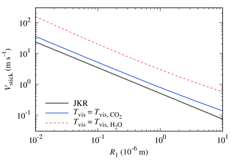
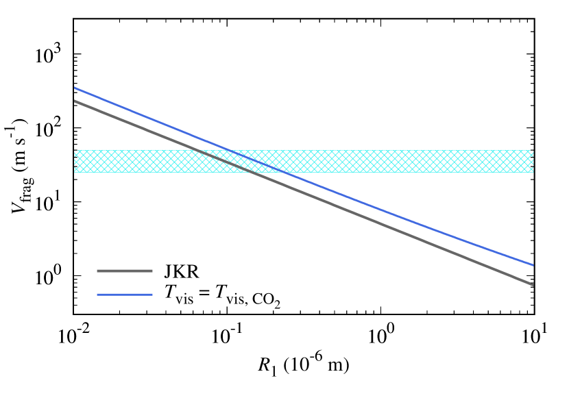
Figure 6: Dependence of the threshold velocity for sticking (for collisions between monomer grains), $V_{\rm stick}$, and the critical velocity for collisional growth/fragmentation (for inter-aggregate collisions), $V_{\rm frag}$, as functions of the particle radius of monomer grains, $R_{1}$. The left panel shows $V_{\rm stick}$ for different assumptions for the size-dependent relaxation time. The red dashed line is $V_{\rm stick}$ for $T_{\rm vis}=T_{\rm vis,\,H_{2}O}$. The blue solid line is $V_{\rm stick}$ for $T_{\rm vis}=T_{\rm vis,\,CO_{2}}$, and this is the standard model in this study. The grey solid line shows $V_{\rm stick,\,JKR}$ as a lower limit of $V_{\rm stick}$. The right panel shows $V_{\rm frag}$ for different assumptions for the size-dependent relaxation time. The blue solid line is $V_{\rm frag}$ for $T_{\rm vis}=T_{\rm vis,\,CO_{2}}$. The grey solid line also shows $V_{\rm frag,\,JKR}$ as a lower limit of $V_{\rm frag}$. In our estimates, $V_{\rm frag}$ is given by $V_{\rm frag}=10V_{\rm stick}$ (Equation 33).

In contrast, the viscoelastic dissipation effects play a great role when $T_{\rm vis}$ is several times higher than that we assumed for CO₂ ice particles. The red dashed line is the threshold velocity for sticking, $V_{\rm stick}$, for the case when $T_{\rm vis}=T_{\rm vis,\,H_{2}O}$ (Equation 28). As $V_{\rm stick}$ is an order of magnitude higher than $V_{\rm stick,\,JKR}$ when we use $T_{\rm vis}=T_{\rm vis,\,H_{2}O}$, we can imagine that the large difference of $V_{\rm stick}$ between CO₂ and H₂O ice particles (Musiolik et al., 2016a, b) mainly originate from the large difference of $T_{\rm vis}$ between two materials.

Pinilla et al. (2017) and Okuzumi & Tazaki (2019) mentioned that the low value of $V_{\rm stick}$ for CO₂ ice particles is due to the small surface free energy of apolar CO₂ ice. However, the literature value of $\gamma_{\rm SV}=80\ {\rm mJ}\ {\rm m}^{-2}$ (Wood, 1999) is comparable to that of H₂O ice, although future direct measurements of the surface free energy of CO₂ ice is essential. In addition, the values of elastic properties, $E$ and $\nu$, are also similar between two materials. Therefore, we proposed that the large difference in $V_{\rm stick}$ between CO₂ and H₂O ice particles is thought to originate from the large difference in $T_{\rm vis}$.

6 Critical Velocity for Collisional Fragmentation of Aggregates

Here we discuss the critical velocity for collisional growth/fragmentation, $V_{\rm frag}$, of dust aggregates composed of $\upmu{\rm m}$-sized monomer grains. The right panel of Figure 6 shows the dependence of $V_{\rm frag}$ on $R_{1}$. Here $R_{1}$ is the radius of monomer grains. The cyan hatched region indicates the maximum collision velocity of dust aggregates in circumstellar disks with weak turbulence, i.e., $25\ {\rm m}\ {\rm s}^{-1}\lesssim V_{\rm col,\,max}\lesssim 50\ {\rm m}\ {\rm s}^{-1}$ (e.g., Adachi et al., 1976; Blum & Wurm, 2008; Wada et al., 2013).

It is empirically known that $V_{\rm frag}$ is an order of magnitude larger than $V_{\rm stick}$ and is almost independent of the number of constituent monomer grains (Dominik & Tielens, 1997; Wada et al., 2009, 2013). Here we briefly explain the basic findings from numerical simulations of collisions of dust aggregates. Based on JKR theory, the amount of energy dissipated in a bouncing collision, $E_{\rm stick,\,JKR}$, is given by (Thornton & Ning, 1998; Wada et al., 2007)

$$E_{\rm stick,\,JKR} = \frac{m^{*}}{2}{V_{\rm stick,\,JKR}}^{2}$$ (30)

$$= 0.9355F_{\rm crit}\delta_{\rm crit},$$

where $F_{\rm crit}=3\pi\gamma R/2$ is the maximum force needed to separate two contact particles and $\delta_{\rm crit}={\left(9/16\right)}^{1/3}\delta_{\rm eq}$ is the critical pulling length between the particles in contact. The energy necessary to break completely a contact in the equilibrium position, $E_{\rm break,\,JKR}$, is slightly larger than $E_{\rm stick,\,JKR}$ (e.g., Wada et al., 2007):

$$E_{\rm break,\,JKR}=1.54F_{\rm crit}\delta_{\rm crit},$$ (31)

and we usually use $E_{\rm break,\,JKR}$ to interpret collision outcomes of dust aggregates.

According to Wada et al. (2013), the critical velocity for collisional growth/fragmentation of dust aggregate of perfectly elastic monomer grains, $V_{\rm frag,\,JKR}$, is empirically given by

$$V_{\rm frag,\,JKR} = C\sqrt{\frac{E_{\rm break,\,JKR}}{m_{1}}}$$ (32)

$$= 0.64C\cdot V_{\rm stick,\,JKR},$$

where $C$ is a dimensionless constant: $C\simeq 15$ for equal-sized collisions and $C\simeq 20$ for different-sized collisions (Wada et al., 2009, 2013). Therefore, the scaling relation between $V_{\rm frag,\,JKR}$ and $V_{\rm stick,\,JKR}$ is approximately given by $V_{\rm frag,\,JKR}=10V_{\rm stick,\,JKR}$. Although it is not clear that whether this relation between $V_{\rm frag}$ and $V_{\rm stick}$ is appliable for dust aggregates of viscoelastic monomer grains (e.g., Gunkelmann et al., 2016), we apply the following assumption to evaluate the value of $V_{\rm frag}$:

$$V_{\rm frag}=10V_{\rm stick}.$$ (33)

The right panel of Figure 6 suggests that $V_{\rm frag}>V_{\rm col,\,max}$ when the radius of monomer grains is $R_{1}\ll 0.1\ \upmu{\rm m}$, and $V_{\rm frag}<V_{\rm col,\,max}$ for the case of $R_{1}\gg 0.1\ \upmu{\rm m}$. In the context of dust growth in circumstellar disks, we usually assumed $R_{1}=0.1\ \upmu{\rm m}$ in numerical calculations (e.g., Okuzumi et al., 2012; Krijt et al., 2015; Homma & Nakamoto, 2018). This assumption is at least consistent with the grain size in the surrounding envelope of proto-stellar objects inferred from near-infrared polarimetry (e.g., Murakawa et al., 2008) and the size distribution of interstellar dust grains (e.g., Mathis et al., 1977; Weingartner & Draine, 2001). For $R_{1}=0.1\ \upmu{\rm m}$, dust aggregates of CO₂ ice monomer grains can stick together without catastrophic fragmentation when the strength of turbulence is weak. In this case, the maximum size of dust aggregates is controlled not by fragmentation but by radial drift (e.g., Okuzumi et al., 2012; Drążkowska & Alibert, 2017), although bouncing and/or erosive collisions between particles with a high mass ratio might prevent dust aggregates from growing into larger aggregates (e.g., Zsom et al., 2010; Krijt et al., 2015). In Section 7.2, we discuss the possible mechanisms for altering the size of monomer grains.

7 Discussion

7.1 Morphology of ice particles used in experiments

We consider that CO₂ ice particles used in Musiolik et al. (2016a) may be monolithic (see Section 5.1). This is because the critical velocity for collisional growth/fragmentation, $V_{\rm frag}$, is several times higher than $0.04\ {\rm m}\ {\rm s}^{-1}$ when we assume that $60\ \upmu{\rm m}$-sized CO₂ ice particles are dust aggregates. If the aggregate radius is $60\ \upmu{\rm m}$, then the radius of monomer grains should be smaller than the half of the aggregate radius, i.e., $R_{1}\lesssim 30\ \upmu{\rm m}$. In this case, $V_{\rm frag,\,JKR}$ of dust aggregates composed of CO₂ ice monomer grains with $R_{1}\lesssim 30\ \upmu{\rm m}$ is

$$V_{\rm frag,\,JKR} = 10V_{\rm stick,\,JKR}$$ (34)

$$= 2.96\times 10^{-1}\ {\left(\frac{R_{1}}{30\ \upmu{\rm m}}\right)}^{-5/6}\ {\rm m}\ {\rm s}^{-1}.$$

Moreover, this large value of $V_{\rm frag,\,JKR}$ gives the minimum estimate of $V_{\rm frag}$. Therefore, the estimated $V_{\rm frag}$ is an order of magnitude higher than the threshold velocity reported by Musiolik et al. (2016a).

We also note that the experimental setup of Musiolik et al. (2016b) is identical to that of Musiolik et al. (2016a). The particle radius of CO₂ and H₂O ices are very similar: $R_{1}=60\ \upmu{\rm m}$ and $90\ \upmu{\rm m}$, respectively. Therefore, we conclude that both CO₂ and H₂O ice particles used in Musiolik et al. (2016a, b) are not aggregates but monolithic grains.

7.2 Size of monomer grains

The size of monomer grains is often taken to $0.1\ \upmu{\rm m}$ (e.g., Okuzumi et al., 2012); however, it is unclear to what extent using a single and constant monomer size is appropriate. Here we discuss several possible scenarios that can alter the size of monomer grains in circumstellar disks.

Ros & Johansen (2013) proposed that condensation of H₂O vapor near the H₂O snow line might be a dominant particle growth mechanism when dust growth is prevented by bouncing and/or fragmentation. If condensation of H₂O vapor controls the size of monomer grains, the physics of heterogeneous nucleation may play a crucial role. Laboratory experiments on heterogeneous nucleation by Iraci et al. (2010) revealed that the formation of a H₂O ice layer on a bare silicate surface requires a substantially high H₂O vapor pressure. Then Ros et al. (2019) showed that H₂O vapor may be deposited predominantly on already ice-covered particles and these icy particles can grow into ${\rm cm}$-sized huge monomer grains near the H₂O snow line. In this scenario, ${\rm cm}$-sized huge monomer grains cannot agglomerate because $V_{\rm stick}$ for ${\rm cm}$-sized huge monomer grains is too low even if they are covered by a H₂O ice mantle. Then icy planetesimals might be formed through gravitational collapse of clumps of ${\rm cm}$-sized icy grains (e.g., Johansen et al., 2007; Bai & Stone, 2010).

This selective condensation process may be important not only near the H₂O snow line but also near the CO₂ snow line. We note, however, that the formation process of the first CO₂ ice layer may different from that of the H₂O ice layer. As CO₂ ice might be formed via chemical reaction of CO and OH on grain surfaces (e.g., Bosman et al., 2018; Krijt et al., 2020), the size of monomer grains covered by a CO₂ ice mantle would be similar to that covered by a H₂O ice mantle near the CO₂ snow line.

Another possible mechanism for changing the size of monomer grains is evaporation and following recondensation of dust particles via flash-heating events (e.g., Miura et al., 2010; Arakawa & Nakamoto, 2016). The flash-heating events in the early solar nebula are thought to be the plausible formation mechanisms of chondrules contained within chondrites (e.g., Arakawa & Nakamoto, 2019). Recently, Fujiya et al. (2019) revealed that at least some chondrite parent bodies were formed beyond the CO₂ snow line, based on C-isotope measurements on carbonate minerals in carbonaceous chondrites. Then the flash-heating events might occur not only in the inner region of the solar nebula but also outside the CO₂ snow line, and the following recondensation process would determine the size of monomer grains in the early solar nebula.

Based on the combination of dust evolution calculations and synthetic polarimetric observations of a circumstellar disk around a young star HL Tau, Okuzumi & Tazaki (2019) revealed that the plausible value of $V_{\rm frag}$ is lower than $1\ {\rm m}\ {\rm s}^{-1}$ both inside the H₂O snow line and outside the CO₂ snow line, to explain the small dust scale height (Pinte et al., 2016) and the observed aggregate radius of $\simeq 100\ \upmu{\rm m}$ (e.g., Kataoka et al., 2017; Stephens et al., 2017) simultaneously. This suggests that the size of monomer grains in the disk around HL Tau might be $R_{1}\gtrsim 10\ \upmu{\rm m}$ (see right panel of Figure 6), and some mechanisms for altering the size of monomer grains from that of interstellar dust grains are required.

7.3 Impact of dust growth on the gas-phase abundance of carbon monoxide in circumstellar disks

Understanding the astrochemistry of CO in circumstellar disks is of great importance in the context of star and planet formation. This is because emission from gas-phase CO and its isotopologues is widely used to study the structures of circumstellar disks, such as the disk radius (e.g., Ansdell et al., 2018), the disk mass (e.g., Ansdell et al., 2016), the temperature profile (e.g., Dullemond et al., 2020), and the presence of giant planets (e.g., Pinte et al., 2019).

It is known that the abundance of CO relative to hydrogen in circumstellar disks decreases by up to factors of 10–100 from its interstellar medium value (e.g., Bergner et al., 2020; Zhang et al., 2020b), and there are a large number of papers which studied chemical processing of CO as the origin of its depletion (e.g., Aikawa et al., 1996; Bergin et al., 2014; Furuya & Aikawa, 2014; Bosman et al., 2018). Physical sequestration of CO ice can also contribute the depletion of gas-phase CO (e.g., Kama et al., 2016; Xu et al., 2017; Krijt et al., 2018). As the vertical settling of large and icy dust aggregates called “pebbles” is the key mechanism of sequestration, dust growth and ensuing radial drift (e.g., Zhang et al., 2020a) are directly associated with the gas-phase abundance of CO. If icy monomer grains are indeed submicron-sized spheres, our results suggest that collisional growth is unlikely to be hindered by fragmentation in the cold outer region of circumstellar disks.

8 Summary

We have investigated the reason for the low threshold velocity for sticking of CO₂ ice particles compared to that of H₂O ice particles. Using the viscoelastic contact model (Krijt et al., 2013), we succeeded in reproducing the experimental results of collisions of CO₂ and H₂O ice particles (Musiolik et al., 2016a, b). Our findings are summarized as follows.

1. For collisons between two viscoelastic spheres, we found that there are three types of collision outcomes, namely, sticking collisions, bouncing collisions, and double collisions. We defined the threshold velocity for sticking, $V_{\rm stick}$, as the transition velocity from double collisions to bouncing collisions (see Figures 1 and 2).

2. In the viscoelastic contact model, the relaxation time, $T_{\rm vis}$, is the key parameter to describe the strength of viscoelastic effects (Krijt et al., 2013). We found that the relaxation time of CO₂ ice particles with the particle radius of $R_{1}=60\ \upmu{\rm m}$ is in the range of $8.5\times 10^{-11}\ {\rm s}\leq T_{\rm vis}\leq 1.97\times 10^{-9}\ {\rm s}$, and $V_{\rm stick}$ of CO₂ ice particles is not so different from that predicted from JKR theory for perfectly elastic spheres (see Figure 3).

3. In contrast, we found that $V_{\rm stick}$ of H₂O ice particles is an order of magnitude higher than that predicted from JKR theory (see Figure 4). The relaxation time of H₂O ice particles with the particle radius of $R_{1}=90\ \upmu{\rm m}$ should be in the range of $5.3\times 10^{-9}\ {\rm s}\leq T_{\rm vis}\leq 2.37\times 10^{-8}\ {\rm s}$, and this value of $T_{\rm vis}$ is an order of magnitude higher than that for CO₂ ice particles. This relaxation time for H₂O ice particles obtained from our numerical results is consistent with the result of Gundlach & Blum (2015) when we use the empirical relation between $T_{\rm vis}$ and $R_{1}$ (see Figure 5).

4. Therefore, we concluded that the large difference in stickiness between H₂O and CO₂ ice particles would mainly originate from the difference in the strength of viscoelastic effects.

5. We also evaluated the critical velocity for collisional growth/fragmentation, $V_{\rm frag}$, of dust aggregates composed of $\upmu{\rm m}$-sized CO₂ ice particles. Assuming that $V_{\rm frag}$ is approximately given by $V_{\rm frag}=10V_{\rm stick}$ and the radius of monomer grains is $R_{1}=0.1\ \upmu{\rm m}$, we found that the maximum size of dust aggregates would be controlled not by fragmentation but by radial drift even outside the CO₂ snow line (see Figure 6).

More broadly, our results highlight the importance of additional energy dissipation channels during collisions of dust particles. Thus future studies on the (viscoelastic) material properties of ices, including H₂O, CO₂, CO, CH₄, CH₃OH, and NH₃, are of great importance to understand the physics and chemistry in circumstellar disks. We also need to study the interplay between dust growth and chemical evolution in circumstellar disks.

Appendix A Dependence of apparent surface energy on crack speed

Greenwood (2004) derived the apparent surface energy which depends on the crack velocity using the Maugis–Dugdale model of the surface force law (Dugdale, 1960; Maugis, 1992). The normalized apparent surface energy and crack velocity, $\beta$ and $v$, are given as functions of $k$ and $\alpha$, where $\alpha$ is the non-dimensional transit time (Greenwood, 2004). For the opening crack, $\beta$ and $v$ are given by

$$\beta = \frac{1}{I_{1}{\left(k,\alpha\right)}},$$ (A1)

$$v = -\frac{\pi}{4}\frac{1}{\alpha{I_{1}{\left(k,\alpha\right)}}},$$ (A2)

and for the closing crack,

$$\beta = \frac{{\left[I_{3}{\left(k,\alpha\right)}\right]}^{2}}{I_{2}{\left(k,\alpha\right)}},$$ (A3)

$$v = \frac{\pi}{4}\frac{1}{\alpha{I_{2}{\left(k,\alpha\right)}}}.$$ (A4)

Here $I_{1}$, $I_{2}$, and $I_{3}$ are given by

$$I_{1}{\left(k,\alpha\right)} = k+{\left(1-k\right)}J_{1}{\left(\alpha\right)},$$ (A5)

$$I_{2}{\left(k,\alpha\right)} = k+{\left(1-k\right)}J_{2}{\left(\alpha\right)},$$ (A6)

$$I_{3}{\left(k,\alpha\right)} = 1-{\left(1-k\right)}J_{3}{\left(\alpha\right)},$$ (A7)

and $J_{1}$, $J_{2}$, and $J_{3}$ are functions of $\alpha$:

$$J_{1}{\left(\alpha\right)} = \frac{1}{2}\alpha\int_{0}^{1}{\rm d}\xi\ \exp{\left[-\alpha{\left(1-\xi\right)}\right]}{F{\left(\xi\right)}},$$ (A8)

$$J_{2}{\left(\alpha\right)} = \frac{1}{2}\alpha\int_{0}^{1}{\rm d}\xi\ \exp{\left[-\alpha{\left(1-\xi\right)}\right]}{A{\left(\xi\right)}},$$ (A9)

$$J_{3}{\left(\alpha\right)} = \frac{1}{2}\int_{0}^{1}{\rm d}\xi\ \exp{\left[-\alpha{\left(1-\xi\right)}\right]}\xi^{-1/2},$$ (A10)

$$F{\left(\xi\right)} = 2\sqrt{\xi}-{\left(1-\xi\right)}\log{\left|\frac{1+\sqrt{\xi}}{1-\sqrt{\xi}}\right|},$$ (A11)

$$A{\left(\xi\right)} = 2\sqrt{\xi}+{\left(1-\xi\right)}\log{\left|\frac{1+\sqrt{\xi}}{1-\sqrt{\xi}}\right|}.$$ (A12)

As both $\beta$ and $v$ are the functions of $\alpha$, we can regard $\alpha$ as an auxiliary variable. Then we obtained $v=v{\left(k,\beta\right)}$ as shown in Figure 7. We also note that Tables 1 and 2 of Greenwood (2004) show the values of $v$ and $\beta$ as functions of $\alpha$, for the case of $k=0.01$. It should be noted that $v$ is defined within the range of $k<\beta<1/k$. For the opening crack, $\beta\to 1/k$ and $v\to-\infty$ when $\alpha\to 0$, and for the closing crack, $\beta\to k$ and $v\to+\infty$ when $\alpha\to 0$.

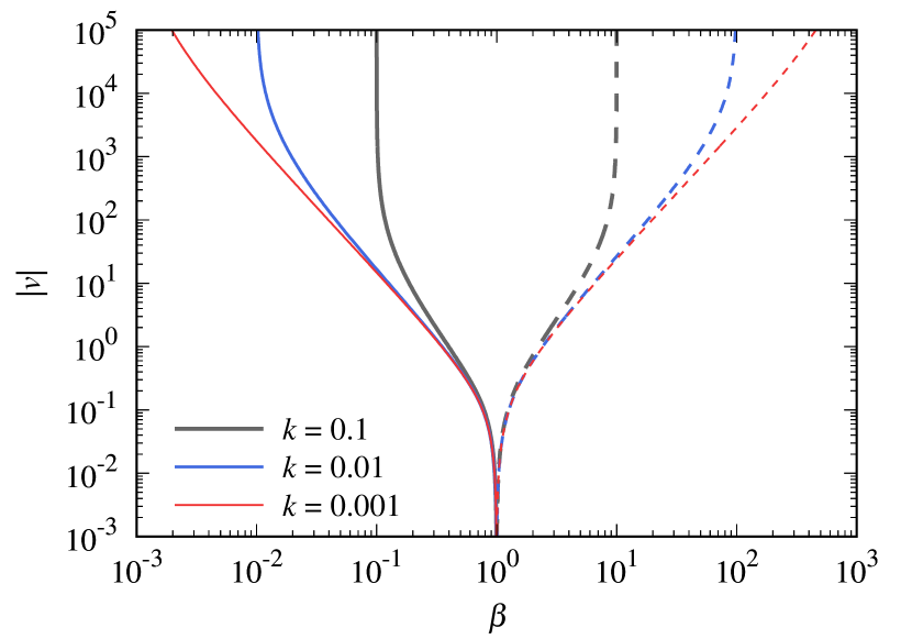
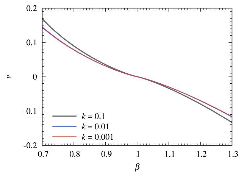
Figure 7: Dependence of the normalized crack velocity, $v$, on the normalized apparent surface energy, $\beta$. The left panel shows $v=v{\left(k,\beta\right)}$ within the range of $10^{-3}<\beta<10^{3}$, and the right panel shows $v=v{\left(k,\beta\right)}$ near $\beta=1$. We note that $v$ is positive (i.e., $\dot{a}>0$) when $\beta<1$ and $v$ is negative when $\beta>1$, and $v=0$ at $\beta=1$ (see Greenwood, 2004).

References

- Adachi et al. (1976) Adachi, I., Hayashi, C., & Nakazawa, K. 1976, Progress of Theoretical Physics, 56, 1756, doi: 10.1143/PTP.56.1756
- Aikawa et al. (1996) Aikawa, Y., Miyama, S. M., Nakano, T., & Umebayashi, T. 1996, ApJ, 467, 684, doi: 10.1086/177644
- Ali-Dib et al. (2014) Ali-Dib, M., Mousis, O., Petit, J.-M., & Lunine, J. I. 2014, ApJ, 793, 9, doi: 10.1088/0004-637X/793/1/9
- Ansdell et al. (2016) Ansdell, M., Williams, J. P., van der Marel, N., et al. 2016, ApJ, 828, 46, doi: 10.3847/0004-637X/828/1/46
- Ansdell et al. (2018) Ansdell, M., Williams, J. P., Trapman, L., et al. 2018, ApJ, 859, 21, doi: 10.3847/1538-4357/aab890
- Arakawa & Nakamoto (2016) Arakawa, S., & Nakamoto, T. 2016, ApJ, 832, L19, doi: 10.3847/2041-8205/832/2/L19
- Arakawa & Nakamoto (2019) —. 2019, ApJ, 877, 84, doi: 10.3847/1538-4357/ab1b3e
- Bai & Stone (2010) Bai, X.-N., & Stone, J. M. 2010, ApJ, 722, 1437, doi: 10.1088/0004-637X/722/2/1437
- Baney & Hui (1999) Baney, J. M., & Hui, C. Y. 1999, Journal of Applied Physics, 86, 4232, doi: 10.1063/1.371351
- Benson & Claxton (1964) Benson, G. C., & Claxton, T. A. 1964, Journal of Physics and Chemistry of Solids, 25, 367, doi: 10.1016/0022-3697(64)90002-2
- Bergin et al. (2014) Bergin, E. A., Cleeves, L. I., Crockett, N., & Blake, G. A. 2014, Faraday Discussions, 168, 61, doi: 10.1039/C4FD00003J
- Bergner et al. (2020) Bergner, J. B., Öberg, K. I., Bergin, E. A., et al. 2020, ApJ, 898, 97, doi: 10.3847/1538-4357/ab9e71
- Blum & Wurm (2000) Blum, J., & Wurm, G. 2000, Icarus, 143, 138, doi: 10.1006/icar.1999.6234
- Blum & Wurm (2008) —. 2008, ARA&A, 46, 21, doi: 10.1146/annurev.astro.46.060407.145152
- Bosman et al. (2018) Bosman, A. D., Walsh, C., & van Dishoeck, E. F. 2018, A&A, 618, A182, doi: 10.1051/0004-6361/201833497
- Brilliantov et al. (2007) Brilliantov, N. V., Albers, N., Spahn, F., & Pöschel, T. 2007, Phys. Rev. E, 76, 051302, doi: 10.1103/PhysRevE.76.051302
- Brilliantov et al. (1996) Brilliantov, N. V., Spahn, F., Hertzsch, J.-M., & Pöschel, T. 1996, Phys. Rev. E, 53, 5382, doi: 10.1103/PhysRevE.53.5382
- Dominik & Tielens (1997) Dominik, C., & Tielens, A. G. G. M. 1997, ApJ, 480, 647, doi: 10.1086/303996
- Drążkowska & Alibert (2017) Drążkowska, J., & Alibert, Y. 2017, A&A, 608, A92, doi: 10.1051/0004-6361/201731491
- Dugdale (1960) Dugdale, D. S. 1960, Journal of Mechanics Physics of Solids, 8, 100, doi: 10.1016/0022-5096(60)90013-2
- Dullemond et al. (2020) Dullemond, C. P., Isella, A., Andrews, S. M., Skobleva, I., & Dzyurkevich, N. 2020, A&A, 633, A137, doi: 10.1051/0004-6361/201936438
- Fujiya et al. (2019) Fujiya, W., Hoppe, P., Ushikubo, T., et al. 2019, Nature Astronomy, 3, 910, doi: 10.1038/s41550-019-0801-4
- Furuya & Aikawa (2014) Furuya, K., & Aikawa, Y. 2014, ApJ, 790, 97, doi: 10.1088/0004-637X/790/2/97
- Glandorf et al. (2002) Glandorf, D. L., Colaprete, A., Tolbert, M. A., & Toon, O. B. 2002, Icarus, 160, 66, doi: 10.1006/icar.2002.6953
- Greenwood (2004) Greenwood, J. A. 2004, Journal of Physics D Applied Physics, 37, 2557, doi: 10.1088/0022-3727/37/18/011
- Gundlach & Blum (2015) Gundlach, B., & Blum, J. 2015, ApJ, 798, 34, doi: 10.1088/0004-637X/798/1/34
- Gundlach et al. (2011) Gundlach, B., Kilias, S., Beitz, E., & Blum, J. 2011, Icarus, 214, 717, doi: 10.1016/j.icarus.2011.05.005
- Gundlach et al. (2018) Gundlach, B., Schmidt, K. P., Kreuzig, C., et al. 2018, MNRAS, 479, 1273, doi: 10.1093/mnras/sty1550
- Gunkelmann et al. (2016) Gunkelmann, N., Ringl, C., & Urbassek, H. M. 2016, A&A, 589, A30, doi: 10.1051/0004-6361/201628081
- Han & Batzle (2004) Han, D.-H., & Batzle, M. L. 2004, Geophysics, 69, 398, doi: 10.1190/1.1707059
- Hayashi (1981) Hayashi, C. 1981, Progress of Theoretical Physics Supplement, 70, 35, doi: 10.1143/PTPS.70.35
- Homma & Nakamoto (2018) Homma, K., & Nakamoto, T. 2018, ApJ, 868, 118, doi: 10.3847/1538-4357/aae0fb
- Iraci et al. (2010) Iraci, L. T., Phebus, B. D., Stone, B. M., & Colaprete, A. 2010, Icarus, 210, 985, doi: 10.1016/j.icarus.2010.07.020
- Israelachvili (2011) Israelachvili, J. N. 2011, Intermolecular and surface forces, 3rd edn. (London: Academic Press), doi: 10.1016/c2011-0-05119-0
- Johansen et al. (2014) Johansen, A., Blum, J., Tanaka, H., et al. 2014, in Protostars and Planets VI, ed. H. Beuther, R. S. Klessen, C. P. Dullemond, & T. Henning, 547, doi: 10.2458/azu_uapress_9780816531240-ch024
- Johansen et al. (2007) Johansen, A., Oishi, J. S., Mac Low, M.-M., et al. 2007, Nature, 448, 1022, doi: 10.1038/nature06086
- Johnson et al. (1971) Johnson, K. L., Kendall, K., & Roberts, A. D. 1971, Proceedings of the Royal Society of London Series A, 324, 301, doi: 10.1098/rspa.1971.0141
- Kama et al. (2016) Kama, M., Bruderer, S., van Dishoeck, E. F., et al. 2016, A&A, 592, A83, doi: 10.1051/0004-6361/201526991
- Kataoka et al. (2017) Kataoka, A., Tsukagoshi, T., Pohl, A., et al. 2017, ApJ, 844, L5, doi: 10.3847/2041-8213/aa7e33
- Kimura et al. (2015) Kimura, H., Wada, K., Senshu, H., & Kobayashi, H. 2015, ApJ, 812, 67, doi: 10.1088/0004-637X/812/1/67
- Kimura et al. (2020) Kimura, H., Wada, K., Kobayashi, H., et al. 2020, MNRAS, 498, 1801, doi: 10.1093/mnras/staa2467
- Krijt et al. (2020) Krijt, S., Bosman, A. D., Zhang, K., et al. 2020, ApJ, 899, 134, doi: 10.3847/1538-4357/aba75d
- Krijt et al. (2014) Krijt, S., Dominik, C., & Tielens, A. G. G. M. 2014, Journal of Physics D Applied Physics, 47, 175302, doi: 10.1088/0022-3727/47/17/175302
- Krijt et al. (2013) Krijt, S., Güttler, C., Heißelmann, D., Dominik, C., & Tielens, A. G. G. M. 2013, Journal of Physics D Applied Physics, 46, 435303, doi: 10.1088/0022-3727/46/43/435303
- Krijt et al. (2015) Krijt, S., Ormel, C. W., Dominik, C., & Tielens, A. G. G. M. 2015, A&A, 574, A83, doi: 10.1051/0004-6361/201425222
- Krijt et al. (2018) Krijt, S., Schwarz, K. R., Bergin, E. A., & Ciesla, F. J. 2018, ApJ, 864, 78, doi: 10.3847/1538-4357/aad69b
- Määttänen et al. (2005) Määttänen, A., Vehkamäki, H., Lauri, A., et al. 2005, Journal of Geophysical Research (Planets), 110, E02002, doi: 10.1029/2004JE002308
- Mangan et al. (2017) Mangan, T. P., Salzmann, C. G., Plane, J. M. C., & Murray, B. J. 2017, Icarus, 294, 201, doi: 10.1016/j.icarus.2017.03.012
- Mathis et al. (1977) Mathis, J. S., Rumpl, W., & Nordsieck, K. H. 1977, ApJ, 217, 425, doi: 10.1086/155591
- Maugis (1992) Maugis, D. 1992, Journal of Colloid and Interface Science, 150, 243, doi: 10.1016/0021-9797(92)90285-t
- Mazzoldi et al. (2008) Mazzoldi, A., Hill, T., & Colls, J. J. 2008, International Journal of Greenhouse Gas Control, 2, 210, doi: 10.1016/s1750-5836(07)00118-1
- Miura et al. (2010) Miura, H., Tanaka, K. K., Yamamoto, T., et al. 2010, ApJ, 719, 642, doi: 10.1088/0004-637X/719/1/642
- Muller et al. (1980) Muller, V. M., Yushchenko, V. S., & Derjaguin, B. V. 1980, Journal of Colloid and Interface Science, 77, 91, doi: 10.1016/0021-9797(80)90419-1
- Murakawa et al. (2008) Murakawa, K., Oya, S., Pyo, T. S., & Ishii, M. 2008, A&A, 492, 731, doi: 10.1051/0004-6361:200810723
- Musiolik et al. (2016a) Musiolik, G., Teiser, J., Jankowski, T., & Wurm, G. 2016a, ApJ, 818, 16, doi: 10.3847/0004-637X/818/1/16
- Musiolik et al. (2016b) —. 2016b, ApJ, 827, 63, doi: 10.3847/0004-637X/827/1/63
- Musiolik & Wurm (2019) Musiolik, G., & Wurm, G. 2019, ApJ, 873, 58, doi: 10.3847/1538-4357/ab0428
- Nachbar et al. (2016) Nachbar, M., Duft, D., Mangan, T. P., et al. 2016, Journal of Geophysical Research (Planets), 121, 753, doi: 10.1002/2015JE004978
- Nagaashi et al. (2018) Nagaashi, Y., Omura, T., Kiuchi, M., et al. 2018, Progress in Earth and Planetary Science, 5, 52, doi: 10.1186/s40645-018-0205-6
- Öberg & Bergin (2020) Öberg, K. I., & Bergin, E. A. 2020, arXiv e-prints, arXiv:2010.03529. https://arxiv.org/abs/2010.03529
- Okuzumi et al. (2016) Okuzumi, S., Momose, M., Sirono, S.-i., Kobayashi, H., & Tanaka, H. 2016, ApJ, 821, 82, doi: 10.3847/0004-637X/821/2/82
- Okuzumi et al. (2012) Okuzumi, S., Tanaka, H., Kobayashi, H., & Wada, K. 2012, ApJ, 752, 106, doi: 10.1088/0004-637X/752/2/106
- Okuzumi & Tazaki (2019) Okuzumi, S., & Tazaki, R. 2019, ApJ, 878, 132, doi: 10.3847/1538-4357/ab204d
- Pinilla et al. (2017) Pinilla, P., Pohl, A., Stammler, S. M., & Birnstiel, T. 2017, ApJ, 845, 68, doi: 10.3847/1538-4357/aa7edb
- Pinte et al. (2016) Pinte, C., Dent, W. R. F., Ménard, F., et al. 2016, ApJ, 816, 25, doi: 10.3847/0004-637X/816/1/25
- Pinte et al. (2019) Pinte, C., van der Plas, G., Ménard, F., et al. 2019, Nature Astronomy, 3, 1109, doi: 10.1038/s41550-019-0852-6
- Planes et al. (2020) Planes, M. B., Millán, E. N., Urbassek, H. M., & Bringa, E. M. 2020, MNRAS, 492, 1937, doi: 10.1093/mnras/stz3631
- Poppe et al. (2000) Poppe, T., Blum, J., & Henning, T. 2000, ApJ, 533, 454, doi: 10.1086/308626
- Quadery et al. (2017) Quadery, A. H., Doan, B. D., Tucker, W. C., Dove, A. R., & Schelling, P. K. 2017, ApJ, 844, 105, doi: 10.3847/1538-4357/aa7890
- Ros & Johansen (2013) Ros, K., & Johansen, A. 2013, A&A, 552, A137, doi: 10.1051/0004-6361/201220536
- Ros et al. (2019) Ros, K., Johansen, A., Riipinen, I., & Schlesinger, D. 2019, A&A, 629, A65, doi: 10.1051/0004-6361/201834331
- Seizinger et al. (2013) Seizinger, A., Krijt, S., & Kley, W. 2013, A&A, 560, A45, doi: 10.1051/0004-6361/201322773
- Shimaki & Arakawa (2012) Shimaki, Y., & Arakawa, M. 2012, Icarus, 221, 310, doi: 10.1016/j.icarus.2012.08.005
- Shuttleworth (1949) Shuttleworth, R. 1949, Proceedings of the Physical Society A, 62, 167, doi: 10.1088/0370-1298/62/3/303
- Sirono & Ueno (2017) Sirono, S.-i., & Ueno, H. 2017, ApJ, 841, 36, doi: 10.3847/1538-4357/aa6fad
- Stephens et al. (2017) Stephens, I. W., Yang, H., Li, Z.-Y., et al. 2017, ApJ, 851, 55, doi: 10.3847/1538-4357/aa998b
- Tabor (1977) Tabor, D. 1977, Journal of Colloid and Interface Science, 58, 2, doi: 10.1016/0021-9797(77)90366-6
- Tatsuuma et al. (2019) Tatsuuma, M., Kataoka, A., & Tanaka, H. 2019, ApJ, 874, 159, doi: 10.3847/1538-4357/ab09f7
- Thornton & Ning (1998) Thornton, C., & Ning, Z. 1998, Powder Technology, 99, 154, doi: 10.1016/s0032-5910(98)00099-0
- Wada et al. (2013) Wada, K., Tanaka, H., Okuzumi, S., et al. 2013, A&A, 559, A62, doi: 10.1051/0004-6361/201322259
- Wada et al. (2007) Wada, K., Tanaka, H., Suyama, T., Kimura, H., & Yamamoto, T. 2007, ApJ, 661, 320, doi: 10.1086/514332
- Wada et al. (2009) —. 2009, ApJ, 702, 1490, doi: 10.1088/0004-637X/702/2/1490
- Weingartner & Draine (2001) Weingartner, J. C., & Draine, B. T. 2001, ApJ, 548, 296, doi: 10.1086/318651
- Wood (1999) Wood, S. E. 1999, PhD thesis, University of California, Los Angeles
- Xu et al. (2017) Xu, R., Bai, X.-N., & Öberg, K. 2017, ApJ, 835, 162, doi: 10.3847/1538-4357/835/2/162
- Yamashita & Kato (1997) Yamashita, Y., & Kato, M. 1997, Geophys. Res. Lett., 24, 1327, doi: 10.1029/97GL01205
- Zhang et al. (2020a) Zhang, K., Bosman, A. D., & Bergin, E. A. 2020a, ApJ, 891, L16, doi: 10.3847/2041-8213/ab77ca
- Zhang et al. (2020b) Zhang, K., Schwarz, K. R., & Bergin, E. A. 2020b, ApJ, 891, L17, doi: 10.3847/2041-8213/ab7823
- Zsom et al. (2010) Zsom, A., Ormel, C. W., Güttler, C., Blum, J., & Dullemond, C. P. 2010, A&A, 513, A57, doi: 10.1051/0004-6361/200912976