Two Component Doublet-Triplet Scalar Dark Matter stabilising the Electroweak vacuum

Abstract

A two component scalar dark matter scenario comprising an additional scalar doublet and a $Y$ = 0 scalar triplet is proposed. Key features of the ensuing dark matter phenomenology are highlighted with emphasis on inter-conversion between the two dark matter components. For suitable choices of the model parameters, we show that such inter-conversion can explain the observed relic abundance when the doublet dark matter component has mass in the desert region while the triplet component has sub-TeV mass. This finding is important in the context of such mass regions known to predict under-abundant relic density for the standalone cases of the scalar doublet and triplet. In addition, we also show that the present scenario can stabilise the electroweak vacuum up to the Planck scale in the parameter space responsible for the requisite dark matter observables.

I Introduction

The discovery of a Higgs boson at the Large Hadron Collider (LHC) Chatrchyan:2012xdj ; Aad:2012tfa completes the particle spectrum of the Standard Model (SM). Moreover, the interactions of the discovered boson to fermions and gauge bosons are in good agreement with the SM predictions. Despite this success, certain shortcomings of the SM on both theoretical and experimental fronts keep the hope for additional dynamics alive and kicking. That the SM alone cannot predict a stable electroweak (EW) vacuum up to the Planck scale for a $t$-quark pole mass at the upper end of its allowed band counts as one such theoretical shortcoming. That is, the SM quartic coupling turns negative while evolving under renormalisation group (RG) thereby destabilising the vacuum and the energy scale where that happens is dictated by the $t$-quark mass chosen Buttazzo:2013uya ; Degrassi:2012ry ; Tang:2013bz ; Ellis:2009tp ; EliasMiro:2011aa . However, augmenting the SM by additional bosonic degrees of freedom (see EliasMiro:2012ay ; Haba:2013lga ; Khan:2014kba ; Khoze:2014xha ; Khan:2015ipa ; Gonderinger:2009jp ; Gonderinger:2012rd ; Chao:2012mx ; Gabrielli:2013hma ; Chakrabarty:2014aya ; Chakraborty:2014oma ; Chakrabarty:2015yia ; Ghosh:2017fmr ; Bhattacharya:2017fid ; Garg:2017iva ; DuttaBanik:2018emv ; Borah:2020nsz for a partial list) can help the Higgs quartic coupling overcome the destabilising effect coming dominantly from the $t$-quark. This motivates to look for extensions of the SM scalar sector. On the experimental front, the SM alone cannot postulate a dark matter (DM) candidate, something whose existence is collectively hinted at by observation of galactic rotation curves Rubin:1970zza , gravitational lensing Clowe:2006eq and anisotropies in the cosmic microwave background. Hitherto the only information known about DM is its relic abundance and is precisely determined by experiments studying anisotropies in cosmic microwave background radiation (CMBR) like Wilkinson Microwave Anisotropy Probe (WMAP) Bennett:2012zja and PLANCK Aghanim:2018eyx . Since these experiments do not shed light on DM spin, the possibility that DM can either be a scalar, a fermion or a vector boson, remains open.

Some attractive scalar DM scenarios are based on augmenting the SM scalar sector by additional scalar $SU(2)_{L}$ multiplets. The most minimal case which in fact transforms trivially under $SU(2)_{L}$ is that of a scalar singlet (an updated analysis is gambit ). However, this scenario interacts with the SM only through the Higgs portal and is tightly constrained. The only mass regions where the scalar singlet accounts for all the observed amount of DM are the Higgs resonance dip and the $\sim$ 1 TeV region, with the former being extremely fine-tuned. We therefore focus on the higher $SU(2)_{L}$ multiplets henceforth that feature gauge interactions.

The next minimal multiplet is an $SU(2)_{L}$ doublet. This is the popular inert doublet model (IDM) whose neutral CP-even/CP-odd component can serve as a DM candidate Deshpande:1977rw ; LopezHonorez:2006gr ; Honorez:2010re ; Belyaev:2016lok ; Choubey:2017hsq ; LopezHonorez:2010tb ; Ilnicka:2015jba ; Arhrib:2013ela ; Cao:2007rm ; Lundstrom:2008ai ; Gustafsson:2012aj ; Kalinowski:2018ylg ; Bhardwaj:2019mts . Despite the popularity, an aesthetically dissatisfying feature of the IDM is the existence of the $M_{\text{DM}}\in[M_{W},500~{}\text{GeV}]$ region, henceforth called desert region which otherwise would have been an interesting range to explore experimentally, wherein only an under-abundant thermal relic density is observed. This underabundance in the desert region is observed precisely because of the DM annihilating to the SM gauge bosons with a huge annihilation cross-section. However for $M_{\text{DM}}\geq 500$ GeV, small mass splittings between the inert scalars, and, an appropriate value for the DM-Higgs portal interaction, the IDM can indeed predict the observed relic abundance. This can be further traced back to cancellations that are triggerred between the s-channel, t-channel and contact interaction terms of the DM DM $\to VV$ amplitude for such near-degeneracy. And in this fashion, the DM DM $\to VV$ annihilation cross section attains the right value for $M_{\text{DM}}\geq 500$ GeV so as to predict a $\simeq$ 0.1 relic density. There have been efforts in the recent past to revive the IDM desert region by augmenting the IDM with additional fields. Some examples involving additional bosons are Bhattacharya:2019fgs (an additional scalar singlet) and Borah:2019aeq ; Keus:2014jha ; Keus:2015xya ; Cordero:2016krd ; Chakrabarty:2015kmt ; Aranda:2019vda ; Keus:2019szx (an additional scalar doublet); while examples involving additional fermions are Borah:2017dfn ; Bhattacharya:2019tqq (right handed neutrinos). With the scalar singlet and doublet extensions of the IDM already in place, an interesting exercise could be to try extending by a scalar $SU(2)_{L}$ triplet. And we choose to take one with $Y$ = 0 in this study, since it is the most minimal scalar triplet in terms of particle content.

A standalone $Y$ = 0 scalar triplet itself can also be a prospective dark multiplet in the inert limitAraki:2011hm ; Fischer:2011zz ; Fischer:2013hwa ; Khan:2016sxm ; Jangid:2020qgo ; Barman:2021ifu ; Bell:2020hnr ; Bandyopadhyay:2020otm ; Ait-Ouazghour:2020slc . A crucial difference between the inert triplet model (ITM) and the IDM is that the former features near-degenerate charged and neutral scalars (the mass splitting being 166 MeV only). In addition to cancellations in DM DM $\to VV$, there are also compulsory coannihilations as a fallout of this near-degeneracy. Therefore, for the model to generate the requisite thermal relic abundance and evade the latest direct detection bound, the DM scalar has to at least have $M_{\text{DM}}\simeq 1.8$ TeV. A wider desert region is thus observed in comparision to the IDM. Therefore, committing to the $Y$=0 scalar triplet scenario annuls the possibility of having of sub-TeV DM. Studies on the stability of the EW vacuum in an IDM and ITM are Khan:2015ipa ; Khan:2016sxm ; Jangid:2020qgo . We mention here that there is likewise the possibility of populating the triplet desert region by injecting additional fields into the theory DuttaBanik:2020jrj .

Since the quantum number(s) of DM cannot be inferred from fundamental principles or available experimental data, the possibility that DM consists of more than one type of particle remains alive. Such a notion was first proposed in Cao:2007fy and has in turn spurred many investigations thereafter, a representative list being Biswas:2013nn ; Fischer:2011zz ; Bhattacharya:2013hva ; Bian:2013wna ; Esch:2014jpa ; Karam:2015jta ; Karam:2016rsz ; Bhattacharya:2016ysw ; DuttaBanik:2016jzv ; Ahmed:2017dbb ; Herrero-Garcia:2017vrl ; Herrero-Garcia:2018qnz ; Poulin:2018kap ; Aoki:2018gjf ; Bhattacharya:2018cgx ; Aoki:2017eqn ; Barman:2018esi ; Chakraborti:2018aae ; Elahi:2019jeo ; Borah:2019aeq ; Bhattacharya:2019fgs ; Biswas:2019ygr ; Bhattacharya:2019tqq ; Nanda:2019nqy ; Maity:2019hre ; Khalil:2020syr ; Belanger:2020hyh ; Nam:2020twn ; DuttaBanik:2020jrj ; DuttaBanik:2020vfr . Such multiparticle DM frameworks open up enticing DM-DM conversion processes that contribute to the thermal relic abundance but not to DM-nucleon scattering as looked for at the direct detection (DD) experiments Akerib:2016vxi ; Aprile:2018dbl ; Tan:2016zwf ; Cui:2017nnn . A multipartite DM scenario therefore can evade the ever tightening bound on the DD rates while enlarging the parameter space compatible with the observed relic density. We propose one such multi-component DM framework in this work that combines the two single component scenarios discussed above, i.e, an inert scalar doublet and a $Y$ = 0 scalar triplet. The key takeaway from the discussion on the IDM and ITM is that certain mass regions in both cases predict underabundant relic densities precisely due to the gauge interaction-mediated co(annihilations). We aim to investigate here if DM-DM conversion can revive these mass regions in the proposed multi-component setup. In other words, the primary motive of this study is to revive the DM mass regions corresponding to the two $SU(2)_{L}$ multiplets that are forbidden in the respective standalone cases. Since these inert multiplets interact with the SM-like doublet via the scalar potential, they tend to aid to EW vacuum stability by generating positive contributions to the RG running of the SM-like quartic coupling. Therefore, we also wish to find out if the parameter space compatible with DM relic density and DD can stabilise the EW vacuum till the Planck scale.

This study is organised as follows. The model is detailed in section II and the relevant constraints are discussed in section III. Section IV throws light on the multi-component DM phenomenology with an emphasis on DM-DM conversion. Section V discusses EW vacuum (meta)stability and comments on the results obtained upon demanding the DM constraints and a (meta)stable vacuum up to the Planck scale together. We conclude in section VI. Important formulae are relegated to the Appendix.

II Model

In the present study, we extend the SM by an $SU(2)_{L}$ scalar doublet $\Phi$ with $Y=\frac{1}{2}$ and a hyperchargeless $SU(2)_{L}$ scalar triplet $\mathcal{T}$. A discrete symmetry $Z_{2}\times Z_{2}^{\prime}$ is introduced under which the SM fields are trivial while the additional scalar multiplets are charged. We provide in Table 1 the quantum numbers of all the scalars in the scenario under both gauge and discrete symmetries. The $Z_{2}\times Z_{2}^{\prime}$ ensures stability of the newly introduced scalar multiplets as a result of which the neutral scalars, if lightest within their respective multiplets, can be DM candidates. Therefore the present setup can accommodate a two component DM scenario. We add that $\Phi$ ($\mathcal{T}$) hereafter can be referred to as inert doublet (triplet) since it does not pick up a vacuum expectation value (VEV) by virtue of the discrete symmetry.

Particle	$SU(2)$	$U(1)_{Y}$	$Z_{2}$	$Z_{2}^{\prime}$
$H$	2	$\frac{1}{2}$	+	+
$\Phi$	2	$\frac{1}{2}$	+	-
$\mathcal{T}$	3	0	-	+

Table 1: Quantum numbers of the SM Higgs doublet $H$ and the inert multiplets $\Phi$ and $\mathcal{T}$.

The most general renormalisable scalar potential consistent with $SU(2)_{L}\times U(1)_{Y}\times Z_{2}\times Z_{2}^{\prime}$ for the given scalar content, $V(H,\Phi,\mathcal{T})$, consists of (i) $V_{H}$: terms involving $H$ alone, (ii) $V_{\Phi}$ : terms involving $\Phi$ alone, (iii) $V_{\mathcal{T}}$: terms involving $\mathcal{T}$ alone and (iv) $V_{\rm{int}}$: interactions involving all $H,~{}\Phi,~{}\mathcal{T}$. That is,

$$V(H,\Phi,\mathcal{T}) = V_{H}+V_{\Phi}+V_{\mathcal{T}}+V_{\text{int}}.$$ (1)

where

$$V_{H} = -\mu_{H}^{2}H^{\dagger}H+\lambda_{H}(H^{\dagger}H)^{2},$$ (2a)

$$V_{\Phi} = \mu_{\Phi}^{2}\Phi^{\dagger}\Phi+\lambda_{\Phi}(\Phi^{\dagger}\Phi)^{2},$$ (2b)

$$V_{\mathcal{T}} = \frac{M_{T}^{2}}{2}~{}{\rm{Tr}}[\mathcal{T}^{2}]+\frac{\lambda_{T}}{4!}(~{}{\rm{Tr}}[\mathcal{T}^{2}])^{2},$$ (2c)

and

$$V_{\rm{int}} = \lambda_{1}(H^{\dagger}H)(\Phi^{\dagger}\Phi)+\lambda_{2}(\Phi^{\dagger}H)(H^{\dagger}\Phi)+\frac{1}{2}\lambda_{3}[(\Phi^{\dagger}H)^{2}+(H^{\dagger}\Phi)^{2}]+\frac{\lambda_{HT}}{2}(H^{\dagger}H)~{}{\rm{Tr}}[\mathcal{T}^{2}]$$ (3)

$$+ \frac{\lambda_{\Phi\mathcal{T}}}{2}(\Phi^{\dagger}\Phi)~{}{\rm{Tr}}[\mathcal{T}^{2}].$$

Following electroweak symmetry breaking (EWSB), the CP-even neutral component of $H$ obtains a VEV $v=246$ GeV. On the other hand, the $Z_{2}$ and $Z_{2}^{\prime}$ ensures that the neutral components of $\Phi$ and $\mathcal{T}$ do not pick up VEVs, as stated before. The scalar fields can then be parameterised as

$$H=\left(\begin{array}[]{c}0\\ \frac{1}{\sqrt{2}}(v+h)\end{array}\right)\,,~{}~{}~{}~{}~{}\Phi=\left(\begin{array}[]{c}H^{+}\\ \frac{1}{\sqrt{2}}(H_{0}+iA_{0})\end{array}\right),\mathcal{T}=\left(\begin{array}[]{c}\ \frac{1}{\sqrt{2}}T_{0}~{}~{}~{}~{}-T^{+}\\ -T^{-}~{}~{}~{}~{}-\frac{1}{\sqrt{2}}T_{0}\end{array}\right),\$$ (10)

and after the EWSB, the masses of the physical scalars are given by

$$m_{h}^{2} = 2\lambda_{H}v^{2},$$

$$m^{2}_{H^{\pm}} = \mu_{\Phi}^{2}+\lambda_{1}\frac{v^{2}}{2},$$

$$m_{H_{0}}^{2} = \mu_{\Phi}^{2}+(\lambda_{1}+\lambda_{2}+\lambda_{3})\frac{v^{2}}{2},$$

$$m_{A_{0}}^{2} = \mu_{\Phi}^{2}+(\lambda_{1}+\lambda_{2}-\lambda_{3})\frac{v^{2}}{2},$$

$$m_{T_{0},T^{\pm}}^{2} = M_{T}^{2}+\frac{\lambda_{HT}}{2}v^{2}.$$ (11)

In Eq.(11), $m_{h}=125.09$ GeV deFlorian:2016spz , is the mass of SM Higgs. The fact that the scalars from the $\Phi$ multiplet have different masses at the tree level itself paves way for the possibility that $H_{0}$ is the lightest and is therefore a DM candidate. Unlike $\Phi$, the charged and neutral members of $\mathcal{T}$ have degenerate masses at the tree level. However, thanks to radiative effects, this degeneracy is lifted at the one-loop level leading to the following mass-splitting.

$$\Delta m = (m_{T^{\pm}}-m_{T_{0}})_{1-\text{loop}}=\frac{\alpha~{}m_{T_{0}}}{4\pi}\bigg{[}f\bigg{(}\frac{M_{W}}{m_{T_{0}}}\bigg{)}$$ (12)

$$- c_{W}^{2}f\bigg{(}\frac{M_{Z}}{m_{T_{0}}}\bigg{)}\bigg{]},$$

where $\alpha$ is the fine structure constant, $M_{W},~{}M_{Z}$ are the masses of the W and Z bosons, $c_{W}=\cos\theta_{W}=M_{W}/M_{Z}$ and $f(x)=-\frac{x}{4}\bigg{[}2x^{3}\rm{ln}(x)+(x^{2}-4)^{3/2}\rm{ln}\bigg{(}\frac{x^{2}-2-x\sqrt{x^{2}-4}}{2}\bigg{)}\bigg{]}$where $x=\frac{M_{W,Z}}{m_{T_{0}}}$. It turns out that in the limit $x\rightarrow 0$ $i.e.$ $m_{T_{0}}\gg$ $M_{W}$ or $M_{Z}$, $f(x)\rightarrow 2\pi x$ and $\Delta m$ can be expressed as Sher:1995tc ; Cirelli:2005uq

$$\Delta m = \frac{\alpha}{2}M_{W}\sin^{2}\frac{\theta_{W}}{2}=166~{}\rm{MeV}.$$ (13)

One now gathers that $T_{0}$ is also stable and can be a DM candidate.

We now turn to identify the independent parameters in this scenario. A counting of parameters in the Lagrangian yields $\{\mu_{H},\mu_{\Phi},M_{T},\lambda_{H},\lambda_{\Phi},\lambda_{T},\lambda_{1},\lambda_{2},\lambda_{3},\lambda_{HT},\lambda_{\Phi T}\}$: 11 parameters. Now, $\mu_{H}$ is eliminated demanding that the Higgs tadpole vanishes. At this level, we invoke $\lambda_{L}\equiv\frac{\lambda_{1}+\lambda_{2}+\lambda_{3}}{2}$ as an independent parameter that quantifies the $H_{0}-H_{0}-h$ portal interaction and hence is of profound importance in a Higgs portal DM scenario such as the IDM. Similarly, $\lambda_{HT}$ parameterises the strength of the $T_{0}-T_{0}-h$ portal coupling and is treated as an independent parameter henceforth. So is $\lambda_{\Phi T}$ since it parameterises the $T_{0}T_{0}\to H_{0}H_{0}$ conversion amplitude. Finally, $\mu_{\Phi},M_{T},\lambda_{1},\lambda_{2}$ and $\lambda_{3}$ can be traded off with the inert masses and $\lambda_{L}$ using

$$\mu^{2}_{\Phi} = m^{2}_{H_{0}}-\lambda_{L}v^{2},$$ (14a)

$$M^{2}_{T} = m^{2}_{T_{0}}-\frac{\lambda_{HT}}{2}v^{2},$$ (14b)

$$\lambda_{1} = 2\lambda_{L}+\frac{2(m^{2}_{H^{+}}-m^{2}_{H_{0}})}{v^{2}},$$ (14c)

$$\lambda_{2} = \frac{m^{2}_{H_{0}}+m^{2}_{A_{0}}-2m^{2}_{H^{+}}}{v^{2}},$$ (14d)

$$\lambda_{3} = \frac{m^{2}_{H_{0}}-m^{2}_{A_{0}}}{v^{2}}.$$ (14e)

The independent parameters in the scalar sector are therefore

$$\{m_{h},m_{H_{0}},m_{A_{0}},m_{H^{\pm}},m_{T_{0}},~{}\lambda_{L},~{}\lambda_{HT},\lambda_{\Phi T},\lambda_{H},\lambda_{\phi},\lambda_{T}\}.$$

In passing, we add that $\lambda_{\Phi}$ and $\lambda_{T}$ parameterise self-interaction within their respective inert sectors and hence are not phenomenologically that much relevant for the ensuing DM analysis. However, these couplings can indeed be constrained from the theoretical requirements of perturbativity, unitarity and positivity of the scalar potential. A detailed discussion can be seen in Section III.

III Constraints

The present scenario is subject to the following theoretical and experimental constraints.

III.1 Theoretical constraints: Perturbativity, positivity of the scalar potential and unitarity

The present model is deemed perturbative if the scalar quartic couplings obey $|\lambda_{i}|\leq 4\pi$. Further, the gauge and Yukawa couplings must also satisfy $|g_{i}|,~{}|y_{i}|\leq\sqrt{4\pi}$.

The introduction of additional scalars opens up additional directions in field space. The following conditions ensure that the potential remains bounded from below (BFB) along each such direction

$$\lambda_{H},~{}\lambda_{T},~{}\lambda_{\Phi}\geq 0,$$ (15a)

$$\lambda_{HT}~{}+~{}\sqrt{\frac{2}{3}\lambda_{H}\lambda_{T}}~{}\geq 0,$$ (15b)

$$\lambda_{1}~{}+~{}2\sqrt{\lambda_{H}\lambda_{\Phi}}~{}\geq 0,$$ (15c)

$$\lambda_{1}~{}+\lambda_{2}~{}-~{}|\lambda_{3}|~{}+2\sqrt{\lambda_{H}\lambda_{\Phi}}~{}\geq 0,$$ (15d)

$$\lambda_{\Phi T}~{}+~{}\sqrt{\frac{2}{3}\lambda_{\Phi}\lambda_{T}}~{}\geq 0.\,\,$$ (15e)

Additional restrictions on the scalar potential come from unitarity. For this model, a couple of $2\to 2$ scattering matrices can be constructed in the basis of neutral and singly charged two-particle states. Unitarity demands that the absolute value of each eigenvalue of these scattering matrices must be $\leq 8\pi$. An element of the scattering matrix is proportional to a quartic coupling in the high energy limit. Following this prescription, one derives for this model

$$|\lambda_{1}\pm\lambda_{2}|\leq 8\pi;~{}~{}~{}|\lambda_{1}\pm\lambda_{3}|\leq 8\pi;~{}~{}~{}|\lambda_{1}+2\lambda_{2}\pm\lambda_{3}|\leq 8\pi;~{}~{}~{}|\lambda_{T}|\leq 24\pi;$$

$$|\lambda_{\Phi T}|\leq 8\pi;~{}~{}|\lambda_{HT}|\leq 8\pi;~{}~{}~{}|\lambda_{H}+\lambda_{\Phi}\pm\sqrt{(\lambda_{H}-\lambda_{\Phi})^{2}+\lambda_{2}^{2}}|\leq 8\pi;$$

$$|\lambda_{H}+\lambda_{\Phi}\pm\sqrt{(\lambda_{H}-\lambda_{\Phi})^{2}+\lambda_{3}^{2}}|\leq 8\pi.$$ (16)

Further, since the present study discusses Higgs vacuum stability, the conditions of perturbativity, positivity of the scalar potential and unitarity have to be met at each intermediate scale while evolving from the EW scale to a higher scale under RG.

III.2 DM observables

For the present scenario to be a successful DM model, the thermal relic abundance it predicts must lie in the observed band. Adopting the latest result from the measurement of relic abundance by the Planck experiment, we demand from our model

$$0.119\lesssim\Omega h^{2}<0.121.$$ (17)

Non-observation of DM-nucleon scattering at the terrestrial experiments have put upper limits on the corresponding cross section as a function of DM mass. We abide by in our study the bound on the spin-independent direct detection (SI-DD) cross section from XENON-1T, the experiment predicting the most stringent bound.

III.3 LHC diphoton signal strength

The dominant amplitude for the $h\to\gamma\gamma$ in the SM reads

$$\mathcal{M}^{\text{SM}}_{h\to\gamma\gamma} = \frac{4}{3}A_{1/2}\Big{(}\frac{M^{2}_{h}}{4M^{2}_{t}}\Big{)}+A_{1}\Big{(}\frac{M^{2}_{h}}{4M^{2}_{W}}\Big{)}.$$ (18a)

We have neglected the small effect of fermions other than the $t$-quark in Eq.(18a). The presence of additional charged scalars in the present framework implies modification to the $h\to\gamma\gamma$ amplitude w.r.t. the SM. This additional scalar contribution reads

$$M^{S}_{h\to\gamma\gamma} = \frac{\lambda_{hH^{+}H^{-}}v}{2m^{2}_{H^{+}}}A_{0}\bigg{(}\frac{m^{2}_{h}}{4m^{2}_{H^{+}}}\bigg{)}+\frac{\lambda_{hT^{+}T^{-}}v}{2m^{2}_{T^{+}}}A_{0}\bigg{(}\frac{m^{2}_{h}}{4m^{2}_{T^{+}}}\bigg{)}$$ (19)

where

$$\lambda_{hH^{+}H^{-}} = \lambda_{1}v,$$ (20a)

$$\lambda_{hT^{+}T^{-}} = \lambda_{HT}v.$$ (20b)

The total amplitude and the decay width then become

$$\mathcal{M}_{h\to\gamma\gamma} = \mathcal{M}^{\text{SM}}_{h\to\gamma\gamma}+\mathcal{M}^{\text{S}}_{h\to\gamma\gamma},$$ (21)

$$\Gamma_{h\to\gamma\gamma} = \frac{G_{F}\alpha^{2}m_{h}^{3}}{128\sqrt{2}\pi^{3}}|\mathcal{M}_{h\to\gamma\gamma}|^{2}.$$ (22)

where $G_{F}$ is the Fermi constant. The various loop functions are listed below Djouadi:2005gj .

$$A_{1/2}(x) = \frac{2}{x^{2}}\big{(}(x+(x-1)f(x)\big{)},$$ (23a)

$$A_{1}(x) = -\frac{1}{x^{2}}\big{(}(2x^{2}+3x+3(2x-1)f(x)\big{)},$$ (23b)

$$A_{0}(x) = -\frac{1}{x^{2}}\big{(}x-f(x)\big{)},$$ (23c)

$$\text{with}~{}~{}f(x) = \text{arcsin}^{2}(\sqrt{x});~{}~{}~{}x\leq 1$$ (23d)

$$=-\frac{1}{4}\Bigg{[}\text{log}\frac{1+\sqrt{1-x^{-1}}}{1-\sqrt{1-x^{-1}}}-i\pi\Bigg{]}^{2};$$

$$x>1.$$

where $A_{1/2}(x),A_{1}(x)$ and $A_{0}(x)$ are loop functions corresponding to spin-$\frac{1}{2}$, spin-1 and spin-0 particles in the loop. The signal strength for the $\gamma\gamma$ channel is defined as

$$\mu_{\gamma\gamma} = \frac{\sigma(pp\to h)\text{BR}(h\to\gamma\gamma)}{\Big{[}\sigma(pp\to h)\text{BR}(h\to\gamma\gamma)\Big{]}_{\text{SM}}}.$$ (24)

Given the inert multiplets do not modify the $pp\to h$ production,

$$\mu_{\gamma\gamma} = \frac{\text{BR}(h\to\gamma\gamma)}{\Big{[}\text{BR}(h\to\gamma\gamma)\Big{]}_{\text{SM}}},$$ (25)

$$\simeq \frac{\Gamma^{\text{SM}}_{h\to\gamma\gamma}}{\Gamma_{h\to\gamma\gamma}}.$$ (26)

In order to ensure that $\mu_{\gamma\gamma}$ lies within the experimental uncertainties, the analysis should respect the latest signal strength from ATLAS Aaboud:2018xdt and CMS Sirunyan:2018koj . The measured value of $\mu_{\gamma\gamma}$ are given by $\mu_{\gamma\gamma}=0.99\pm 0.14$ from ATLAS and $\mu_{\gamma\gamma}=1.17\pm 0.10$ from CMS. The constraints have been imposed at 2$\sigma$.

III.4 Disappearing charged track

The smallness of the mass-splitting between $T^{+}$ and $T_{0}$ implies that the $T^{+}\to T_{0}\pi^{+}$ decay width is tiny. The parent particle $T^{+}$ will therefore travel a macroscopic distance ($\mathcal{O}$(1cm)) before decaying thereby leading to multiple hits in the LHC tracking devices. In addition, the $\pi^{+}$ would be too soft to be detected. As a result, a disappearing charged track (DCT) signal would be seen. The lighter is $T^{+}$, the higher is the $pp\to T^{+}T^{-}$ production cross section at the LHC and hence, the higher would be the number of DCT events. It then follows that non-observation of such events at the LHC would lead to lower bounds on the mass of $T^{+}$. It was shown recently Chiang:2020rcv that non-observation of DCT signals at the 13 TeV, integrated luminosity (L) = 36 fb^-1 excludes a real triplet scalar lighter than 275 GeV. The reach can extend to 590 GeV and 745 GeV with L = 300 fb^-1 and 3000 fb^-1 respectively. We have therefore maintained $m_{T^{+}}>$ 275 GeV throughout the analysis in light of the current constraint.

III.5 Oblique parameters

The additional scalars present in this setup can induce potentially important contributions to the oblique ($S,T,U$) parameters That is, for $X=S,T,U$, one can write

$$\Delta X = \Delta X_{\text{ID}}+\Delta X_{\text{IT}},$$ (27)

where the subscripts ID (IT) denotes the contribution from the inert doublet (triplet). We have for the inert doublet,

$$\Delta S_{\text{ID}} = \frac{1}{2\pi}\bigg{[}\frac{1}{6}\ln\bigg{(}\frac{m_{H_{0}}^{2}}{m_{H^{\pm}}^{2}}\bigg{)}-\frac{5}{36}+\frac{m_{H_{0}}^{2}m_{A_{0}}^{2}}{3(m_{A_{0}}^{2}-m_{H_{0}}^{2})^{2}}+\frac{m_{A_{0}}^{4}(m_{A_{0}}^{2}-3m_{H_{0}}^{2})}{6(m_{A_{0}}^{2}-m_{H_{0}}^{2})^{3}}\ln\bigg{(}\frac{m_{A_{0}}^{2}}{m_{H_{0}}^{2}}\bigg{)}\bigg{]},$$ (28a)

$$\Delta T_{\text{ID}} = \frac{1}{16\pi s^{2}_{W}M_{W}^{2}}\Big{[}F(m^{2}_{H^{+}},m^{2}_{H_{0}})+F(m^{2}_{H^{+}},m^{2}_{A_{0}})-F(m^{2}_{H_{0}},m^{2}_{A_{0}})\Big{]},$$ (28b)

$$\Delta U_{\text{ID}} = 0.$$ (28c)

In the above,

$$F(x,y) = \frac{x+y}{2}-\frac{xy}{x-y}~{}{\rm ln}\bigg{(}\frac{x}{y}\bigg{)}~{}~{}~{}{\rm for}~{}~{}~{}x\neq y\,,$$ (29)

$$= 0~{}~{}~{}{\rm for}~{}~{}~{}x=y.$$

While for the inert triplet,

$$\Delta S_{\text{IT}} = 0,$$ (30a)

$$\Delta T_{\text{IT}} = \frac{1}{16\pi s^{2}_{W}M_{W}^{2}}F(m^{2}_{T^{+}},m^{2}_{T_{0}}),$$ (30b)

$$\simeq \frac{(\Delta m)^{2}}{24\pi s^{2}_{W}M_{W}^{2}}~{}~{}~{}~{}~{}\text{since $\Delta m<<m_{T_{0}}$},$$ (30c)

$$\Delta U_{\text{IT}} = -\frac{1}{3\pi}\bigg{[}m_{T_{0}}^{4}\rm{ln}\bigg{(}\frac{m_{\it{T}_{\rm 0}}^{2}}{m_{\it{T^{\pm}}}^{2}}\bigg{)}\frac{(3m_{\it{T^{\pm}}}^{2}-m_{\it{T}_{\rm 0}}^{2})}{(m_{\it{T}_{\rm 0}}^{2}-m_{\it{T^{\pm}}}^{2})^{3}}+\frac{5(m_{\it{T}_{\rm 0}}^{4}+m_{\it{T^{\pm}}}^{4})-22m_{\it{T}_{\rm 0}}^{2}m_{\it{T^{\pm}}}^{2}}{6(m_{\it{T}_{\rm 0}}^{2}-m_{\it{T^{\pm}}}^{2})^{2}}\bigg{]}$$

$$\simeq \frac{\Delta m}{3\pi~{}m_{T^{\pm}}}$$

The most updated bounds read Zyla:2020zbs

$$\Delta S=0.02\pm 0.10,~{}~{}\Delta T=0.07\pm 0.12,~{}~{}\Delta U=0.00\pm 0.09.$$ (31)

The stated bounds have been imposed at 2$\sigma$ in our analysis. A few comments are in order. First, the contribution of an inert real scalar triplet to the oblique parameters is found to be at most $\mathcal{O}$ $\big{(}\frac{\Delta m}{m_{T_{0}}}\big{)}$ or further suppressed. The contributions are therefore negligible in comparison to the corresponding ones from the inert doublet. Secondly, a non-zero $T$-parameter indicates that the $\rho$-parameter deviates from unity at one-loop (since the doublets and the VEVless triplet present in this model predict $\rho$ = 1 at tree level.). However, ensuring that $T$ stays within the stipulated bound is tantamount to obeying the $\rho$-parameter constraint.

IV Dark Matter phenomenology

The present setup being a two component DM scenario, has the discrete symmetry $Z_{2}\times Z_{2}^{\prime}$ that remain unbroken throughout and guarantee the stability of the DM candidates. To find the individual contributions to the relic density, one requires to evaluate the yields of both the DM species by solving coupled Boltzmann equations. In order to do so, first we identify all the relevant annihilation and coannihilation channels of both, (we refer the reader Bhattacharya:2019tqq and DuttaBanik:2020jrj where all such channels for IDM and ITM are listed respectively). Apart from these, diagrams responsible for DM-DM conversion are shown in Fig.1 assuming $m_{T_{0}}>m_{H_{0}}$. This inter-conversion of the two DM particles plays a significant role in our analysis and in turn, makes the set of Boltzmann equations coupled. Next to calculate the DM relic abundance, we implement the model file in LanHEP Semenov:2014rea and then pass the files generated in the LanHEP to the micrOMEGAS Belanger:2014vza . For inspecting the current scenario, we consider the all constraints discussed in section III.

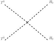
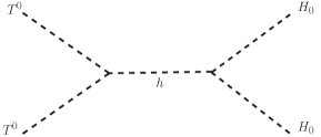
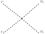
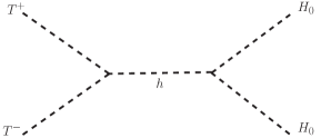
Figure 1: DM-DM conversion channels, assuming $m_{T_{0}}>m_{H_{0}}$.

IV.1 Relic Density

In order to obtain the comoving number densities of the both the DM particles, one needs to solve a set of coupled Boltzmann equation in the present setup as the conversion of one DM to another plays a non-trivial role. Due to the involvement of two DM particles, it is always better to redefine the usual $x$ parameter from $\frac{m_{\rm{DM}}}{\tilde{T}}$ to $\frac{\mu_{\text{DM}}}{\tilde{T}}$, where $\mu_{\text{DM}}$ is nothing but the reduced mass expressed as: $~{}\mu_{\text{DM}}=\frac{m_{H_{0}}m_{T_{0}}}{m_{H_{0}}+m_{T_{0}}}$ whereas $\tilde{T}$ represents the temperature of the Universe. Finally, we write the coupled Boltzmann equations in terms of parameter $x=\frac{\mu_{\text{DM}}}{\tilde{T}}$ and the co-moving number density $Y_{\rm DM}=n_{\rm DM}/s$ ($s$ being the entropy density) redefined as $y_{i}$ $i=H_{0},T_{0}$) via $y_{i}=0.264M_{Pl}\sqrt{g_{*}}\mu Y_{i}$, as below

$$\frac{dy_{H_{0}}}{dx} = \frac{-1}{x^{2}}\bigg{[}\langle\sigma v_{H_{0}H_{0}\rightarrow XX}\rangle\left(y_{H_{0}}^{2}-(y_{H_{0}}^{EQ})^{2}\right)~{}+~{}\langle\sigma v_{H_{0}H_{0}\rightarrow T_{0}T_{0}}\rangle\left(y_{H_{0}}^{2}-\frac{(y_{H_{0}}^{EQ})^{2}}{(y_{T_{0}}^{EQ})^{2}}y_{T_{0}}^{2}\right)\Theta(m_{H_{0}}-m_{T_{0}})$$ (32a)

$$-~{}\langle\sigma v_{T_{0}T_{0}\rightarrow H_{0}H_{0}}\rangle\left(y_{T_{0}}^{2}-\frac{(y_{T_{0}}^{EQ})^{2}}{(y_{H_{0}}^{EQ})^{2}}y_{H_{0}}^{2}\right)~{}\Theta(m_{T_{0}}-m_{H_{0}})\bigg{]},$$

$$\frac{dy_{T_{0}}}{dx} = \frac{-1}{x^{2}}\bigg{[}\langle\sigma v_{T_{0}T_{0}\rightarrow XX}\rangle\left(y_{T_{0}}^{2}-(y_{T_{0}}^{EQ})^{2}\right)~{}+~{}\langle\sigma v_{T_{0}T_{0}\rightarrow H_{0}H_{0}}\rangle\left(y_{T_{0}}^{2}-\frac{(y_{T_{0}}^{EQ})^{2}}{(y_{H_{0}}^{EQ})^{2}}y_{H_{0}}^{2}\right)\Theta(m_{T_{0}}-m_{H_{0}})$$ (32b)

$$-~{}\langle\sigma v_{H_{0}H_{0}\rightarrow T_{0}T_{0}}\rangle\left(y_{H_{0}}^{2}-\frac{(y_{H_{0}}^{EQ})^{2}}{(y_{T_{0}}^{EQ})^{2}}y_{T_{0}}^{2}\right)\Theta(m_{H_{0}}-m_{T_{0}})\bigg{]}.$$

One can relate $y_{i}^{EQ}$ in the same way as $y_{i}$ via $y_{i}^{EQ}=0.264M_{Pl}\sqrt{g_{*}}\mu_{\text{DM}}Y_{i}^{EQ}$, where $Y_{i}^{EQ}$ is the equilibrium density $Y_{i}^{EQ}$ defined in terms of $\mu_{\text{DM}}$ as

$$Y_{i}^{EQ}(x)=0.145\frac{g}{g_{*}}x^{3/2}\bigg{(}\frac{m_{i}}{\mu_{\text{DM}}}\bigg{)}^{3/2}e^{-x\big{(}\frac{m_{i}}{\mu_{\text{DM}}}\big{)}}.$$ (33)

Here $M_{\rm Pl}=1.22\times 10^{19}~{}{\rm GeV}$, $g_{*}=106.7$, $m_{i}=m_{H_{0}},m_{T_{0}}$, $X$ represents all the SM particles, $H^{\pm},A_{0}$ and $T^{\pm}$, and finally, the thermally averaged effective annihilation cross-section inclusive of both the annihilation and DM-DM conversion processes can be expressed as

$$\langle\sigma v\rangle=\frac{1}{8m^{4}_{i}\tilde{T}K_{2}^{2}(\frac{m_{i}}{T})}\int\limits^{\infty}_{4m_{i}^{2}}\sigma(s-4m_{i}^{2})\sqrt{s}K_{1}\bigg{(}\frac{\sqrt{s}}{\tilde{T}}\bigg{)}ds,$$ (34)

and is evaluated at $\tilde{T}_{f}$. The freeze-out temperature $\tilde{T}_{f}$ can be derived by equating the DM interaction rate $\Gamma=n_{\rm DM}\langle\sigma v\rangle$ with the expansion rate of the universe $H(\tilde{T})\simeq\sqrt{\frac{\pi^{2}g_{*}}{90}}\frac{T^{2}}{M_{\rm Pl}}$. In Eq.(34), $K_{1,2}(x)$ represents the modified Bessel functions. Finally, in Eq.(32), $\Theta$ function is used in order to explain the conversion process (corresponding to Fig.1) of one DM to another which strictly depends on the mass hierarchy of DM particles.

At this stage, it is perhaps pertinent to mention that $H^{\pm}$ (heavier than $H_{0}$) and $T^{\pm}$ (heavier than $T_{0}$) are expected to be in equilibrium with the thermal plasma by virtue of their electromagnetic interactions as well as their interactions with the Higgs. Apart from being in equilibrium, the $H^{+}$ can decay into $H_{0}l^{+}\bar{\nu}$ and $T^{+}$ can decay to $T_{0}\pi^{+}$ via off-shell $W$-bosons. Finally $A_{0}$ being heavier than $H_{0}$ can always decay to $H_{0}$ and the SM fermions via an off shell $Z$. The heavier scalars within the dark multiplets are thus not cosmologically stable. These coupled equations now have to be solved numerically to find the asymptotic abundance of the DM particles, $y_{i}\left(\frac{\mu_{\text{DM}}}{m_{i}}x_{\infty}\right)$, which can be further used to calculate the relic density:

$$\Omega_{i}h^{2} = \frac{854.45\times 10^{-13}}{\sqrt{g_{*}}}\frac{m_{i}}{\mu_{\text{DM}}}y_{i}\left(\frac{\mu_{\text{DM}}}{m_{i}}x_{\infty}\right),$$ (35)

where $x_{\infty}$ indicates a very large value of $x$ after decoupling. Total DM relic abundance is then given as

$$\Omega_{\rm Total}{h}^{2}=\Omega_{T_{0}}{h}^{2}+\Omega_{H_{0}}{h}^{2}\,\,.$$ (36)

It is to be noted that total relic abundance must satisfy the DM relic density obtained from Planck Aghanim:2018eyx

$$\Omega_{\rm Total}{h}^{2}=0.1199{\pm 0.0027}\,.$$ (37)

IV.2 Direct and Indirect detection

Experiments like LUX Akerib:2016vxi , PandaX-II Tan:2016zwf ; Cui:2017nnn and Xenon-1T Aprile:2017iyp ; Aprile:2018dbl look for signals of DM-nucleon scattering. And, non-observation of the same have led to upper bounds on the DM-nucleon scattering cross-section as a function of DM mass. It must be added that, in principle, inelastic direct detection scatterings can also get triggered in case the mass gap between the DM and the next heavier particle within the multiplet is below $\sim$ 150 keV Arina:2009um . Being a two component DM scenario, in the present model both the DM particles would appear in direct search experiments. However, one should take into account the fact that direct detection cross sections of both are to be rescaled by the corresponding relic density fractions. Hence, the effective direct detection cross-section of triplet scalar DM $T_{0}$ is given as Ayazi:2015mva

$$\sigma_{\rm{T_{0},eff}}=\frac{\Omega_{T_{0}}}{\Omega_{\rm Total}}\frac{\lambda_{HT}^{2}}{4\pi}\frac{1}{m_{h}^{4}}f^{2}\frac{m_{N}^{4}}{(m_{T_{0}}+m_{N})^{2}},$$ (38)

and similarly the effective direct detection cross-section of $H_{0}$ is expressed as Borah:2019aeq

$$\sigma_{\rm{H_{0},eff}}=\frac{\Omega_{H_{0}}}{\Omega_{\rm Total}}\frac{\lambda_{L}^{2}}{4\pi}\frac{1}{m_{h}^{4}}f^{2}\frac{m_{N}^{4}}{(m_{H_{0}}+m_{N})^{2}}\,,$$ (39)

where $m_{N}$ is the nucleon mass, $\lambda_{HT}$ and $\lambda_{L}$ are the quartic couplings involved in the DM-Higgs interaction. A recent estimate of the Higgs-nucleon coupling ($f$) gives $f=0.32$ Giedt:2009mr . We provide below the Feynman diagrams for the spin independent elastic scattering of DM with nucleon.

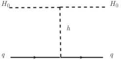
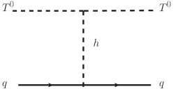
Figure 2: Spin independent elastic scattering of DM-nucleon.

On the other hand, indirect search experiments like Fermi-LAT MAGIC:2016xys also offer promising prospects of detecting WIMP DM candidates. Annihilation of DM to SM particles, especially to photons and neutrinos, plays a crucial role here. Since photons and neutrinos are electrically neutral, they have a higher chance of reaching the detector without getting deflected. The effective indirect detection cross section $\sigma^{\text{ID}}_{\text{i,eff}}$ in a multicomponent DM setup relates to the computed cross section $\sigma^{\text{ID}}_{\text{i}}$ as Bhattacharya:2019fgs ; Betancur:2020fdl

$$\sigma^{\text{ID}}_{\text{i,eff}} = \bigg{(}\frac{\Omega_{i}}{\Omega_{\text{Total}}}\bigg{)}^{2}\sigma^{\text{ID}}_{\text{i}}.$$ (40)

The exponent 2 in $\big{(}\frac{\Omega_{i}}{\Omega_{\text{Total}}}\big{)}^{2}$ in case of indirect detection can be explained using the fact that there are two annihilating DM particles in the initial state as opposed to one in case of direct detection. We demand that $\sigma^{\text{ID}}_{\text{i,eff}}$ obey the upper bound from Fermi-LAT for $i=H_{0},T_{0}$.

IV.3 Result

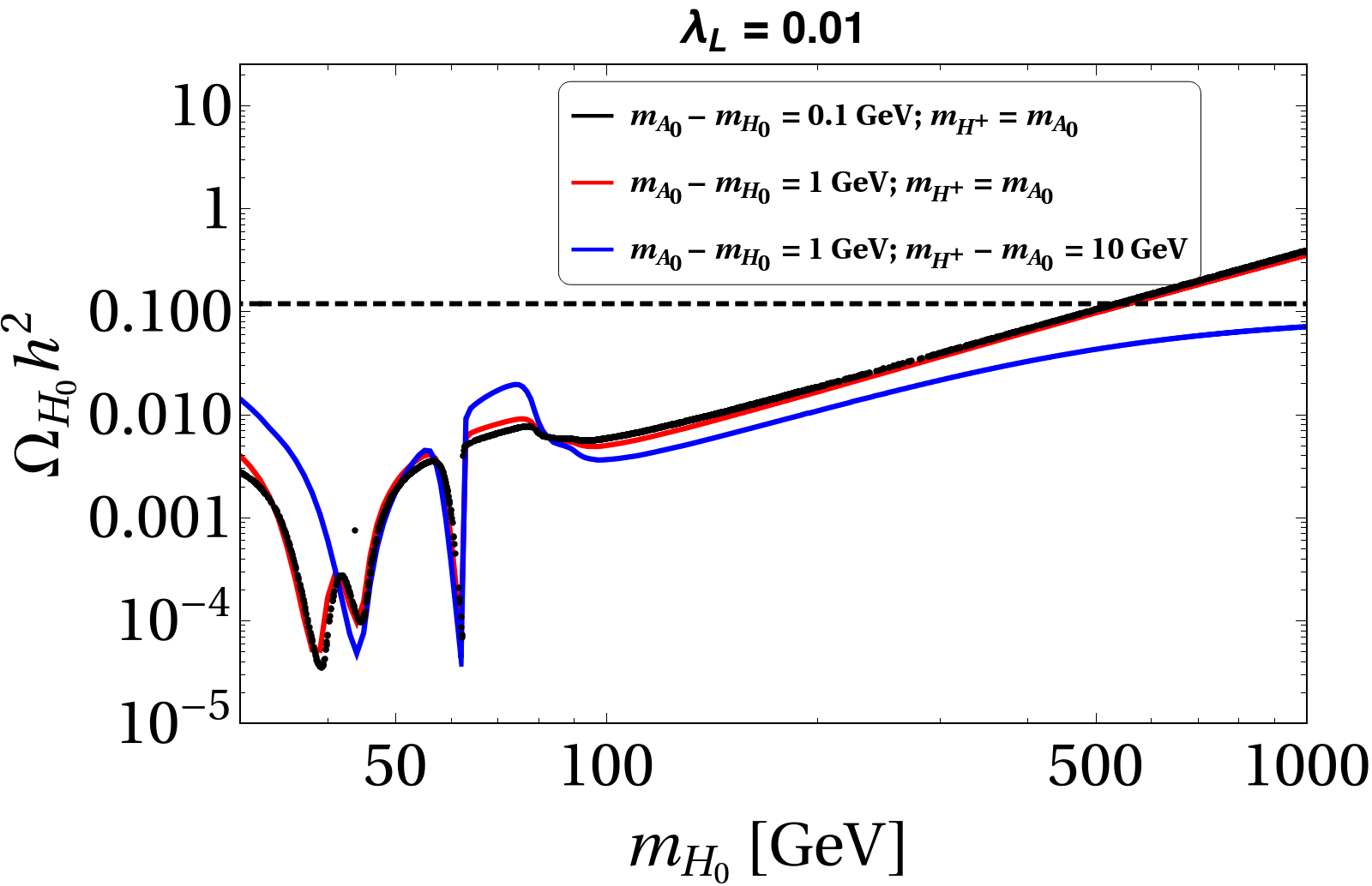
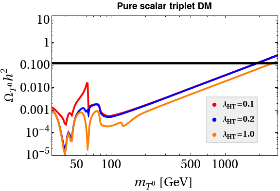
Figure 3: Left Panel: The relic density of the inert doublet for $m_{H^{+}}=m_{A_{0}}$ and $m_{H^{+}}=m_{A_{0}}+10$ GeV. Right Panel: Variation of $\Omega_{T_{0}}h^{2}$ versus $m_{T_{0}}$ for different values of $\lambda_{HT}$.

The phenomenologies of the single component IDM LopezHonorez:2006gr ; Honorez:2010re ; Belyaev:2016lok ; Choubey:2017hsq ; LopezHonorez:2010tb ; Ilnicka:2015jba ; Arhrib:2013ela ; Cao:2007rm ; Lundstrom:2008ai ; Gustafsson:2012aj ; Kalinowski:2018ylg ; Bhardwaj:2019mts as well as ITM Araki:2011hm ; Fischer:2011zz ; Fischer:2013hwa ; Khan:2016sxm ; Jangid:2020qgo ; Barman:2021ifu ; Bell:2020hnr are well known. Despite being allowed by the direct search experiments, both fail to predict the observed for a substantial range of the DM mass. While this under-abundant region extends from $M_{W}$ to 500 GeV for the IDM, the same is in fact larger for the ITM. In this case, the under-abundant region extends till 1.8 TeV of the DM mass (irrespective of the choices of their Higgs portal couplings as their impact on the relic density is sub-dominant) particularly because, apart from its usual annihilations to SM gauge bosons, it must co-annihilate to the gauge bosons with the help of its charged partners $T^{\pm}$ (mass splitting is very small $i.e.~{}\Delta m=166~{}\text{MeV}$). This in turn makes the effective annihilation cross-section of the triplet DM quite large and hence, leading to under-abundance of the relic density for a wider range of the DM mass as compared to the IDM. We comment on the role of the portal coupling $\lambda_{HT}$ here. The co(annihilations) are heavily gauge coupling-driven and the dependence on $\lambda_{HT}$ is subleading. To show this, we plot the triplet relic density for $\lambda_{HT}$ = 0.1, 0.2, 1 in the right panel of Fig. 3. It is seen that $\Omega_{T_{0}}$ for $\lambda_{HT}$ = 0.1, 0.2 differ only slightly away from the $h$-resonance (our region of interest in $m_{T_{0}}\gtrsim$ 750 GeV). For $\lambda_{HT}$ = 1, though there appears to be sizeable difference, we can still say that the role of the $h$-mediated annihilation is subleading compared to the gauge-driven annihilatons. This can be understood from the following example. Increasing $\lambda_{HT}$ from 0.2 to 1 increases the $h$-mediated annihilation cross section 25-fold. However, the relic density for $m_{T_{0}}$ = 1.8 TeV drops only by a factor $\sim$ 2. This shows that the contribution of the gauge-driven (co)annihilation is way higher. Despite this subleading impact of $\lambda_{HT}$, a large $\sim$ 1 value for the former can still deplete the relic density by $\simeq$ 50$\%$ (w.r.t. $\lambda_{HT}$ = 0.2). This depletion is something we do not aim for and therefore, restrict $\lambda_{HT}$ in the [0.1,0.2] interval henceforth. And for such a choice, the $T_{0}T_{0},~{}T^{+}T^{-}\to H_{0}H_{0}$ conversion is dominated by the $T^{+}-T^{-}-H_{0}-H_{0}$ and $T_{0}-T_{0}-H_{0}-H_{0}$ contact interactions and not by the s-channel $h$-exchange.

In order to maximise the relic density from the inert doublet, we choose $m_{H^{\pm}}=m_{A_{0}}$. With $m_{H^{\pm}}\neq m_{A_{0}}$, this contribution will be accordingly less. We have demonstrated this in the left panel of Fig.3 by comparing the relic densities corresponding to $m_{H^{+}}=m_{A_{0}}$ and $m_{H^{+}}=m_{A_{0}}$ + 10 GeV. The gap thereby made in the total relic density will then have to be compensated by the scalar triplet. Given a heavier $T_{0}$ tends to predict a higher $\Omega_{T_{0}}$, the parameter region for $\lambda_{2}\neq\lambda_{3}$ would prefer an accordingly heavier $T_{0}$. This is contrary to our objective of accomplishing a lighter $T_{0}$ (By ”lighter”, we imply lighter than what is seen in the single component triplet dark matter scenario.).

In the present study, we aim to find out if inter-conversion (which depends on their mass hierarchy though) of one DM species to another can possibly revive such mass regions of IDM and ITM that are known to yield under-abundant thermal relic abundance. As stated before, the relevant parameters that would control the study are $m_{H_{0}},m_{A_{0}},m_{H^{\pm}},\lambda_{L},\lambda_{HT}$ and $\lambda_{\Phi T}$. For the analysis purpose, we only stick to mass regime $100~{}{\rm{GeV}}\leq m_{H_{0}}\leq 500~{}{\rm{GeV}}$ and $100~{}{\rm{GeV}}\leq m_{T_{0}}\leq 2000~{}{\rm{GeV}}$ for the doublet and the triplet respectively. As the Higgs portal couplings of both the DM do not play much significant role the in obtaining the correct total relic density for the given choice of the parameter space, we fixed the portal couplings $\lambda_{L}=0.01$ and $\lambda_{HT}=0.15$. Even though the role of the portal couplings is subleading in the DM phenomenology, they play a non-trivial role in stabilizing the electroweak vacuum which will be discussed in detail in section V.

In Figs.4(a) and 4(b), we show the variation of the individual relic density contributions, $\Omega_{H_{0}}h^{2}$ and $\Omega_{T_{0}}h^{2}$, against their respective masses, $m_{H_{0}}$ and $m_{T_{0}}$, such that the the total relic density ($\Omega_{Total}h^{2}$) defined in Eq.(36) satisfies the Planck limit Aghanim:2018eyx . A combined plot is Fig.4(c). In the same plot we also show the effect of different choices of the coupling $\lambda_{\Phi T}$ (involved in DM-DM conversion as shown in Fig.1) on the parameter space. Here, we choose three different values of $\lambda_{\Phi T}$ for illustration, i.e., $\lambda_{\Phi T}=0,0.5$ and $1.0$.

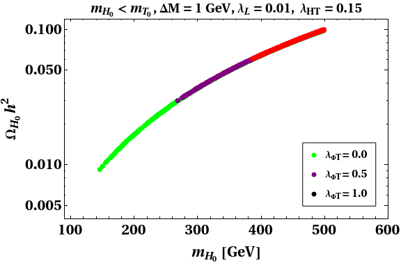
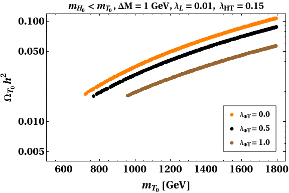
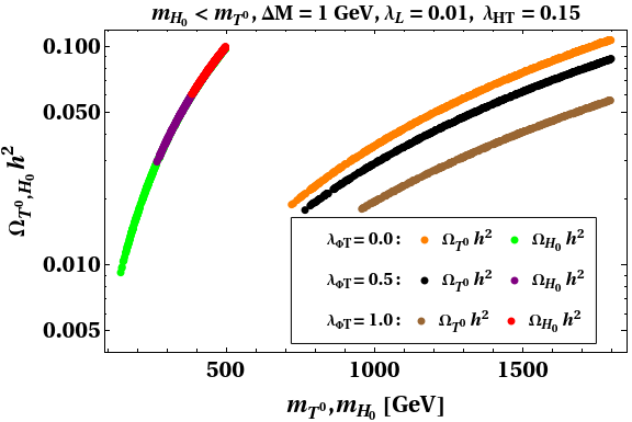
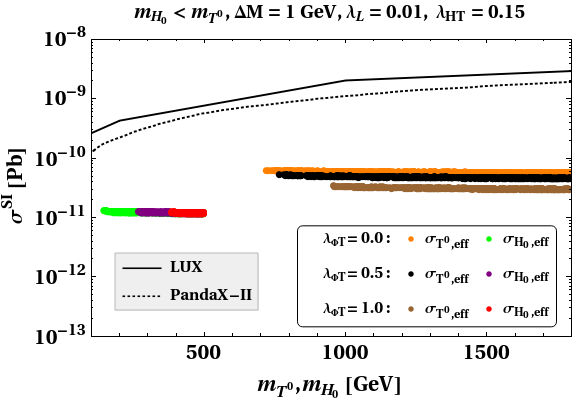
Figure 4: Points that satisfy the correct total DM relic abundance for $\lambda_{HT}=0.15$, $\lambda_{L}=0.01$, $\Delta M=1$ GeV and different values of $\lambda_{\Phi T}$ while maintaining $m_{T_{0}}>m_{H_{0}}$ in the (a) $m_{H_{0}}-\Omega_{H_{0}}h^{2}$ plane and (b) $m_{T_{0}}-\Omega_{T_{0}}h^{2}$ plane. Panel (c) combines the plots in panels (a) and (b). And panel (d) shows the corresponding Spin independent DM-nucleon scattering cross-sections corresponding to the points in (c). Limits from direct detection experiments are shown in black solid lines (LUX), dotted (PandaX-II) and dashed (XENONnT).

The respective variations of the relic densities versus the DM masses with different $\lambda_{\Phi T}$ are indicated by (i) orange (for $T_{0}$) and green (for $H_{0}$) patches for $\lambda_{\Phi T}=0$, (ii) black (for $T_{0}$) and purple (for $H_{0}$) patches for $\lambda_{\Phi T}=0.5$ and (iii) brown (for $T_{0}$) and red (for $H_{0}$) patches for $\lambda_{\Phi T}=1.0$. Here, for our analysis purpose we also define mass splitting among the inert doublet components as $\Delta M=m_{H^{\pm}}-m_{H_{0}}=m_{A_{0}}-m_{H_{0}}$ and fix its value at 1 GeV. Such a choice of the $\Delta M$ is motivated from the fact that the maximum contribution from the single component IDM to relic density can be obtained for such small mass splittings only LopezHonorez:2006gr ; Honorez:2010re ; Belyaev:2016lok ; Choubey:2017hsq ; LopezHonorez:2010tb ; Ilnicka:2015jba ; Arhrib:2013ela ; Cao:2007rm ; Lundstrom:2008ai ; Gustafsson:2012aj ; Kalinowski:2018ylg ; Bhardwaj:2019mts . It is to be noted that the inelastic direct detection processes are ruled out in the IDM for such a mass splitting. In case of the inert triplet also, the mass gap $m_{T^{+}}-m_{T_{0}}$ = 166 MeV is too large to trigger the $W$-mediated inelastic scattering $T_{0}T^{+}\to\bar{q}q^{\prime}$.

We would like to elucidate on Fig.4 a bit. One must note that $\Omega_{H_{0}}h^{2}$ and $\Omega_{T_{0}}h^{2}$ in the figure obey $\Omega_{H_{0}}h^{2}+\Omega_{T_{0}}h^{2}$ = Observed relic $\simeq$ 0.12 (the variation within the PLANCK band ignored here for the sake of understanding). For instance, for $\lambda_{\Phi T}$ = 0.5, $\Omega_{H_{0}}h^{2}$ for a particular $m_{H_{0}}$ can be read from the violet curve. The corresponding $\Omega_{T_{0}}h^{2}$ is then approximately equal to 0.12 - $\Omega_{H_{0}}h^{2}$ and one can then read the corresponding $m_{T_{0}}$ value on the X-axis. This implies that the relic densities of the rightmost point on the violet curve and the leftmost point on the black curve add up to $\simeq$ 0.12. This is how Fig.4 should be read.

To understand the non-triviality of the conversion coupling in the present set up, we begin with the case where $\lambda_{\Phi T}=0$. Note that with $\lambda_{\Phi T}=0$, although conversion via process shown in diagram Fig.1(a) does not contribute, however the processes $T^{+}T^{-},T_{0}T_{0}\rightarrow H_{0}H_{0}$ can still take place due to the non-zero values of $\lambda_{L}$ and $\lambda_{HT}$ via the one in Fig.1(b). Here, we observe that when $\Omega_{T_{0}}h^{2}$ is small (corresponding to lowest point of the orange patch), the dominant contribution towards the total relic density comes from $\Omega_{H_{0}}h^{2}$ (top most point of the green patch which lies below the red patch) so as to satisfy the total relic density with the Planck limit. Similarly a farthest point on the orange patch corresponds to the lowest point of the green one. As an example, for $m_{T_{0}}=785~{}\rm{GeV}$ we get $\Omega_{T_{0}}h^{2}=0.019$ (almost $15\%$ of the total relic density), rest of the $85\%$ of the total relic density comes from $\Omega_{H_{0}}h^{2}$ which corresponds to a single point on the green patch with $m_{H_{0}}=498$ GeV and $\Omega_{H_{0}}h^{2}=0.098$.

Upon turning on the conversion coupling (say $\lambda_{\Phi T}=0.5$), a shift in the relic densities of both the DM candidates is observed (see the black and the purple patches in Fig.4). The reason behind this is easy to understand. When the conversion coupling is switched on, the $T_{0}$ starts converting to $H_{0}$ and hence the relic density of the $T_{0}$ decreases whereas we observe an upward shift for the relic density $\Omega_{H_{0}}$ (the purple patch). A similar behavior is observed for $\lambda_{\Phi T}=1.0$ where the relic density of $T_{0}$ is further decreased and the relic density of $H_{0}$ is increased, we notice that the red patch has now became much smaller. This is because the maximum contribution towards the total relic density from $T_{0}$ can at most be $53\%$ (with $m_{T_{0}}=1790$ GeV, $\Omega_{T_{0}}h^{2}=0.060$) which in turn requires $\Omega_{H_{0}}h^{2}=0.056$ (rest of the $47\%$ contribution towards the total relic density) for $m_{H_{0}}=387$ GeV leading to a shrinking in the red patch. In Fig.4(d), we plot the effective direct detection cross-section of both the DM with respect to their respective masses and compare it with the experimental results obtained from LUX Akerib:2016vxi , PandaX-II Tan:2016zwf ; Cui:2017nnn and XENONnT XENON:2020kmp for different values of $\lambda_{\Phi T}$ (similar to Fig.4(a)). Here it is interesting to point out that, although the current setup is allowed from the constraints coming from present direct search experiments like LUX Akerib:2016vxi and PandaX-II Tan:2016zwf ; Cui:2017nnn , the parameter space of the setup can come in tension with the XENONnT projections. However, this is actually a positive finding since this renders the model testable and hence falsifiable in a future experiment. Considering the Fig.4(a) and the bounds from the present direct search results from Fig.4(d) together, we can conclude that the parameter space under consideration is allowed from both the relic density as well as the direct detection constraints. For better understanding, we also tabulate the result discussed above in Table 2 for three different choices of the conversion couplings $\lambda_{\Phi T}=0.0,0.5$ and 1.0.

$\lambda_{\Phi T}$	$m_{H_{0}}$ [GeV]	$m_{T_{0}}$ [GeV]	$~{}\Omega_{H_{0}}h^{2}$	$~{}\Omega_{T_{0}}h^{2}$
0.0	500	730	0.0981	0.0192
	147	1799	0.0092	0.1070
0.5	500	770	0.0988	0.0180
	280	1799	0.0320	0.0875
1.0	500	1000	0.0993	0.0194
	388	1799	0.0606	0.0568

Table 2: Table showing the relic densities for certain sample mass values for different $\lambda_{\Phi T}$. We have taken $\lambda_{L}=0.01$ and $\lambda_{HT}=0.15$.

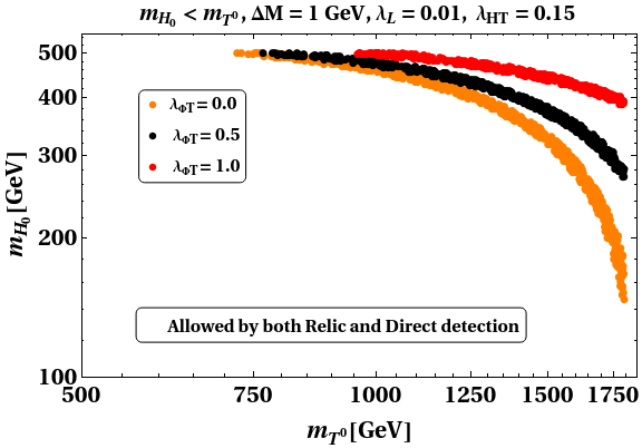
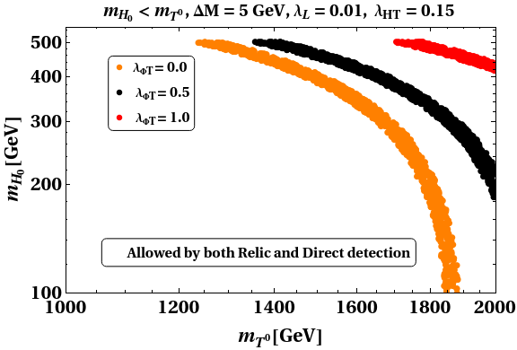
Figure 5: All the points which satisfy the correct total DM relic abundance and are also allowed by direct detection for different values of $\lambda_{\Phi T}$ while maintaining $m_{T_{0}}>m_{H_{0}}$ for $\lambda_{HT}=0.15$ and (a) $\Delta M=1$ GeV, (b) $\Delta M=5$ GeV in $m_{H_{0}}-m_{T_{0}}$ plane.

Finally, in Fig.5, we incorporate parameter region plots in the $m_{H_{0}}-m_{T_{0}}$ plane for $\Delta M$ = 1 GeV (left panel), 5 GeV (right panel). All the points in this case are allowed by the relic density and direct detection constraints. The effect of the conversion coupling discussed in Fig.4(a) becomes prominent in Fig.5. Looking at the left panel of Fig.5, one may notice that almost the entire desert mass regime of the single component IDM and $m_{T_{0}}$ in the range $700~{}{\rm{GeV}}\leq m_{T_{0}}\leq 2~{}{\rm{TeV}}$ (The relic density of a $Y$=0 triplet being underabundant for $m_{T_{0}}<$ 1.8 TeV) now becomes allowed in the two component set up, thanks to DM-DM conversion. However, for the higher value $\Delta M$ = 5 GeV we observe in the right panel that $m_{T_{0}}$ shifts towards the heavier side. This happens because with the increase in the mass splitting among the inert doublet components, the contribution of $\Phi$ to the total relic density decreases and hence in order for total relic density to satisfy the Planck limit, the triplet contribution has to increase which can only result from an accordingly larger mass of the triplet DM.

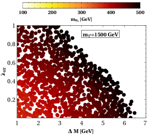
Figure 6: Variation of Triplet-Higgs portal coupling ($\lambda_{HT}$) with inert doublet mass splitting ($\Delta M$) for a fixed value of $m_{T_{0}}=1500$ GeV. Colour bar shows the variation with $m_{H_{0}}$.

Although the effect of the Higgs portal coupling $\lambda_{HT}$ is subleading in the present scenario, a small effect of its variation can be observed in the parameter space when we vary the mass splitting among the inert doublet components. We try to demonstrate this subleading behaviour via a heat plot in Fig.6. For a fixed $m_{T_{0}}$, the annihilation rate of the scalar triplet increases upon increasing $\lambda_{HT}$ thereby causing $\Omega_{T_{0}}h^{2}$ to drop, albeit mildly. Since the total relic density is demanded to lie in the Planck band, $\Omega_{H_{0}}h^{2}$ must accordingly increase to fill the gap. And that is possible only for a higher inert doublet DM mass. And since, the larger the $m_{H_{0}}$, the darker is the shade, one expects a darkening of the points as one moves up the $\lambda_{HT}$ axis. This is exactly what is observed in Fig.6 where a gradual darkening is seen as one moves up from the bottom left to the top left corner. On the other hand, as $\Delta M$ increases, $\Omega_{H_{0}}h^{2}$ tends to decrease for a given $m_{H_{0}}$. If $\lambda_{HT}$ is held fixed, one then has to then increase $m_{H_{0}}$ to maintain the original $\Omega_{H_{0}}h^{2}$. A darkening of the points is then expected as one moves towards the right of the $\Delta M$ axis. An inspection of the figure corroborates this when such a darkening is immediately seen.

Prior to ending this section, we comment on the consequences of an $m_{H_{0}}>m_{T_{0}}$ hierarchy. Here the processes responsible for DM conversion will now be reversed and the inert doublet is expected to be responsible for the production of the second dark matter $T_{0}$ i.e. $H_{0}H_{0}\to T_{0}T_{0}$. As mentioned before, a sub-TeV scalar triplet always leads to an under abundant relic due to high co(annihilation) rates to gauge boson final states. Given that we restrict $m_{H_{0}}<$ 500 GeV in this study, demanding $m_{H_{0}}>m_{T_{0}}$ at the same time implies that even the $H_{0}H_{0}\to T_{0}T_{0}$ conversion does not suffice to generate the observed relic. Therefore, the $m_{H_{0}}>m_{T_{0}}$ hierarchy is not appealing from the two component DM perspective and we shall not consider it any further.

V EW vacuum stability and combined analysis

This section discusses the role of the additional scalar multiplets in (meta)stabilising the EW vacuum. For high field values, i.e., $h>>v$, the RG improved effective potential for this scenario can be expressed as Degrassi:2012ry

$$V^{\rm{eff}}_{H} \simeq \frac{\lambda^{\rm{eff}}_{H}(h)}{4}h^{4},$$ (41)

where $\lambda^{\rm{eff}}_{H}(\mu)=\lambda_{H}(\mu)+\lambda^{\rm{SM,eff}}_{H}(\mu)+\lambda^{\Phi,\rm{eff}}_{H}(\mu)+\lambda^{\rm{T,eff}}_{H}(\mu)$. Here, $\lambda^{\rm{SM,eff}}_{H}(\mu)$ is the contribution coming from the SM fields to $\lambda_{H}$ whereas $\lambda^{\rm{\Phi,eff}}_{H}(\mu)$ and $\lambda^{\rm{T,eff}}_{H}(\mu)$ are the contributions from $\Phi$ and $T$ respectively. The EW boundary scale from which the couplings start evolving is chosen to be the $t$-quark pole mass $M_{t}$ = 173.34 GeV. All the running couplings are to be evaluated at a scale $\mu=h$ in Eq.(41). One derives the following.

$$\lambda^{\rm{\Phi,eff}}_{H}(\mu) = e^{4\Gamma(\mu)}\frac{1}{16\pi^{2}}\bigg{[}2\frac{\lambda_{1}^{2}}{4}\bigg{(}\rm{ln}\frac{\lambda_{1}}{2}-\frac{3}{2}\bigg{)}+\frac{(\lambda_{1}+\lambda_{2}+\lambda_{3})^{2}}{4}\bigg{(}\rm{ln}\frac{\lambda_{1}+\lambda_{2}+\lambda_{3}}{2}-\frac{3}{2}\bigg{)}$$ (42)

$$+\frac{(\lambda_{1}+\lambda_{2}-\lambda_{3})^{2}}{4}\bigg{(}\rm{ln}\frac{\lambda_{1}+\lambda_{2}-\lambda_{3}}{2}-\frac{3}{2}\bigg{)}\bigg{]},$$

$$\lambda^{\rm{T,eff}}_{H}(\mu) = e^{4\Gamma(\mu)}\frac{1}{16\pi^{2}}\bigg{[}\frac{3\lambda^{2}_{HT}}{4}\bigg{(}\text{ln}\frac{\lambda_{HT}}{2}-\frac{3}{2}\bigg{)}\bigg{]}.$$ (43)

Here, $\Gamma(\mu)=\int_{M_{t}}^{\mu}\gamma(\mu^{\prime})~{}\rm{d~{}ln(\mu^{\prime})}$ and $\gamma(\mu)$ denotes the anomalous dimension of the Higgs field Buttazzo:2013uya . By virtue of such quantum effects, a second minima can show up at high energy scales. The condition $\lambda^{\text{eff}}_{H}(\mu)>0$ ensures that the EW minimum is deeper than the second minimum, that is, a stable EW vacuum. On the other hand, $\lambda^{\text{eff}}_{H}(\mu)<0$ implies that the second minimum is deeper. The fate of the EW vacuum in this case is decided by computing the probability of tunnelling to the second vacuum. The expression for the tunnelling probability is given by

$$\mathcal{P}_{T} = (\mu_{B}T_{U})^{4}e^{-\frac{8\pi^{2}}{3\lambda_{H}(\mu_{B})}}.$$ (44)

In Eq.(44), $T_{U}$ is the age of the universe and $\mu_{B}$ denotes the scale at which the tunneling probability is maximized, determined from $\beta_{\lambda_{H}}(\mu_{B})$ = 0. The EW vacuum is metastable if the tunnelling lifetime is greater than the universe’s age. With this, one obtains the following criterion on $\lambda^{\text{eff}}_{H}(\mu)$:

$$\lambda^{\text{eff}}_{H}(\mu) > \frac{-0.065}{1-\text{ln}(v/\mu_{B})}.$$ (45)

The following boundary values are then taken for the SM Yukawa and gauge couplings Buttazzo:2013uya .

$$y_{t}(M_{t}) = 0.93690+0.00556\times(M_{t}-173.34)-0.00042\times(\alpha_{s}(M_{Z})-0.1184)/0.0007,$$

$$g_{1}(M_{t}) = 0.35830+0.00011\times(M_{t}-173.34)-0.00020\times(M_{W}-80.384)/0.014,$$ (46b)

$$g_{2}(M_{t}) = 0.64779+0.00004\times(M_{t}-173.34)+0.00011\times(M_{W}-80.384)/0.014,$$ (46c)

$$g_{3}(M_{t}) = 1.1666-0.00046\times(M_{t}-173.34)+0.00314\times(\alpha_{s}(M_{Z})-0.1184)/0.0004.$$ (46d)

We take $M_{W}$ = 80.384 GeV and $\alpha_{s}(M_{Z})$ = 0.1184. The input values of $\lambda_{1},\lambda_{2}$ and $\lambda_{3}$ are determined using Eqs. (14c)-(14e).

The expression for $\beta_{\lambda_{H}}$ in Eq.(47a) tells us that the quartic couplings the vacuum instability (or metastability) scale is sensitive to are $\lambda_{1-3}$ and $\lambda_{HT}$. The sample points (SPs) listed in Table 3 demonstrate this sensitivity.

SP	$m_{H_{0}}$	$m_{T_{0}}$	$\lambda_{HT}$	$\Delta M$	$\mu_{\gamma\gamma}$	$\Omega_{T_{0}}h^{2}$	$\Omega_{H_{0}}h^{2}$	$\sigma_{T_{0},eff}$ ($pb$)	$\sigma_{H_{0},eff}$($pb$)	$\sigma^{\text{ID}}_{T_{0},eff}$($cm^{3}/s$)	$\sigma^{\text{ID}}_{H_{0},eff}$($cm^{3}/s$)
SP1	$400$	$1426$	0.1	$1$	0.999	$0.056$	$0.064$	$2.01\times 10^{-11}$	$1.2\times 10^{-11}$	$7.1\times 10^{-28}$	$1.2\times 10^{-26}$
SP2	$400$	$1426$	0.15	$1$	0.999	$0.056$	$0.064$	$4.5\times 10^{-11}$	$1.2\times 10^{-11}$	$7.1\times 10^{-28}$	$1.2\times 10^{-26}$
SP3	$400$	$1426$	0.2	$1$	0.999	$0.056$	$0.064$	$8.1\times 10^{-11}$	$1.2\times 10^{-11}$	$7.0\times 10^{-28}$	$1.2\times 10^{-26}$
SP4	$400$	$1670$	0.15	$5$	0.997	$0.076$	$0.044$	$4.5\times 10^{-11}$	$8.0\times 10^{-12}$	$2.1\times 10^{-27}$	$5.3\times 10^{-27}$
SP5	$400$	$1856$	0.15	$10$	0.994	$0.093$	$0.025$	$4.5\times 10^{-11}$	$4.6\times 10^{-12}$	$5.9\times 10^{-27}$	$1.7\times 10^{-27}$

Table 3: Sample points predicting a total relic density within the Planck band that are also allowed by the theoretical, direct detection, indirect detection and diphoton signal strength constraints. All masses and mass-splittings are in GeV.

We choose $\lambda_{L}$ = 0.01, $\lambda_{\Phi T}=0.5$, $\lambda_{\phi}=0.001$ and $\lambda_{T}=0.001$ throughout the analysis using RG. It is noted that the SP1-3 differ only in their values of $\lambda_{HT}$. Since (co)annihilation in the triplet sector is heavily driven by gauge interactions, tuning $\lambda_{HT}$ in the interval [0.1,0.2] changes $\Omega_{T_{0}}$ only slightly. The corresponding RG trajectories of $\lambda_{H}^{\text{eff}}$ is shown in the left panel of Fig.7. It is seen that though $\lambda_{H}^{\text{eff}}$ turns negative in each case, it remains within the metastable band. In addition, the larger the input value of $\lambda_{HT}$, the higher is the scale at which $\lambda_{H}^{\text{eff}}$ turns negative. As mentioned before, this is solely due to the presence of the $\mathcal{O}(\lambda_{HT}^{2})$ term in $\beta_{\lambda_{H}}$. While SP4 and SP5 are primarily characterized by their values of $\Delta M$, the $m_{T_{0}}$ values are also different for each. This is because a decrease in $\Omega_{H_{0}}$ that inevitably occurs with an increasing $\Delta M$ in these sample points is counterbalanced by an increased contribution from the triplet, something in turn achieved by appropriately raising $m_{T_{0}}$. Now, with $\lambda_{L}$ fixed, increasing $\Delta M$ accordingly increases the magnitudes of $\lambda_{1-3}$ at the EW scale. This in turn generates an upward push to the RG trajectory of $\lambda_{H}^{\text{eff}}$ via the $\lambda_{1-3}$-dependent terms in $\beta_{\lambda_{H}}$. Since SP2, SP4 and SP5 feature different $\Delta M$ values for the same $\lambda_{HT}$, we show the corresponding RG evolution curves in the right panel of Fig.7 in order to confirm the impact of changing $\Delta M$. A metastable EW vacuum is identified for $\Delta M$ = 1 GeV. Increasing the same to $\Delta M$ = 5 GeV and 10 GeV stabilises the same up to the Planck scale.

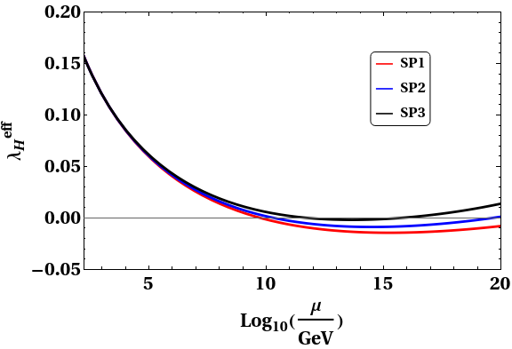
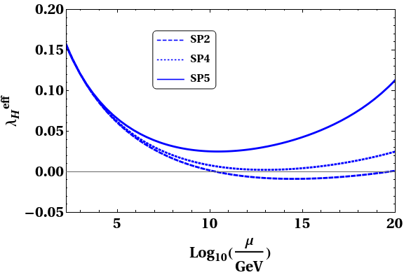
Figure 7: RG evolution of $\lambda_{H}^{\text{eff}}$ for the SPs. In the left panel for SP1, SP2 and SP3 the values for $\{\lambda_{1},~{}\lambda_{2},~{}\lambda_{3}\}=\{0.046,-0.013-0.013\}$ while in the right panel for SP4 $\{\lambda_{1},~{}\lambda_{2},~{}\lambda_{3}\}=\{0.153,~{}-0.066,~{}-0.066\}$ and for SP5 $\{\lambda_{1},~{}\lambda_{2},~{}\lambda_{3}\}=\{0.287,~{}-0.134,~{}-0.134\}$.

The bands corresponding to metastable and stable EW vacuum sketched in the $m_{T_{0}}-m_{H_{0}}$ plane are shown in Fig.8. Also, the parameter region predicting the requisite relic density and compatible with the direct detection constraints is overlaid on the same. Upon inspection, it is seen that the parameter plane mostly favours metastability over stability for $\lambda_{HT}$ = 0.1 and $\Delta M$ = 5 GeV. And this is attributed to the EW scale values of $\lambda_{1},\lambda_{2}$ $\lambda_{3}$ and $\lambda_{HT}$ that are not sizeable enough to stabilise the vacuum till $M_{\text{Pl}}$ for most part of the $m_{T_{0}}-m_{H_{0}}$ plane. In fact, a stable vacuum is ruled out for $m_{H_{0}}\lesssim$ 480 GeV. With increasing $\lambda_{HT}$ to 0.15, the band corresponding to stability expands to include $m_{H_{0}}\gtrsim 360$ GeV. This is expected for the following reason. For a higher $\lambda_{HT}$, accordingly smaller $|\lambda_{1}|,|\lambda_{2}|$ and $|\lambda_{3}|$ suffice to ensure a stable vacuum up to $M_{\text{Pl}}$. And with $\lambda_{L}$ and $\Delta M$ fixed, smaller $|\lambda_{1}|,|\lambda_{2}|$ and $|\lambda_{3}|$ imply a smaller $m_{H_{0}}$. We also remark that the parameter region compatible with the DM constraints changes only slightly with this change in $\lambda_{HT}$ since the (co)annihilations of the triplet scalars are mostly driven by the gauge interactions. Demanding the requisite relic abundance rules out $m_{T_{0}}\lesssim 1.35$ TeV for $\Delta M$ = 5 GeV.

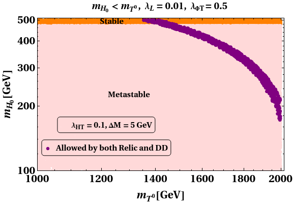
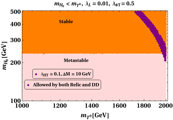
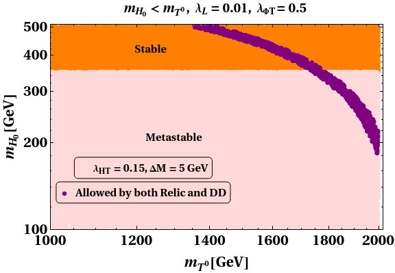
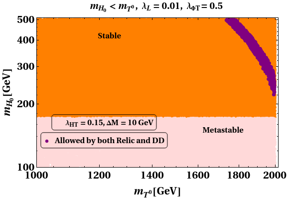
Figure 8: Parameter region compatible with (meta)stable vacuum and the DM observables in the $m_{T_{0}}-m_{H_{0}}$ plane. The orange (pink) bands correspond to stability (metastability). The blue region is allowed by the DM constraints.

As illustrated before in Fig.7, increasing $\Delta M$ while keeping $\lambda_{L}$ unchanged aids vacuum stability by increasing the magnitudes of $\lambda_{1},\lambda_{2}$ and $\lambda_{3}$. In other words, with a higher $\Delta M$, the requisite magnitudes of these quartic couplings at the input scale required to stabilise the EW vacuum up to the Planck scale can be achieved for an accordingly lower $m_{H_{0}}$. This is concurred by the plot with $\lambda_{HT}$ = 0.1 and $\Delta M$ = 10 GeV in which case the stability band includes $m_{H_{0}}\gtrsim 240$ GeV. In addition, the DM-compatible region also changes appreciably with respect to $\Delta M$ = 5 GeV. With now a higher mass-splitting in the inert doublet sector, $\Omega_{H_{0}}$ diminishes. Heavier triplet scalars are needed to fill up the deficit in relic density compared to what occurs for $\Delta M$ = 5 GeV. This is the reason why the DM-compatible region shifts towards right in the $m_{T_{0}}-m_{H_{0}}$ plane when switching from $\Delta M$ = 5 GeV to 10 GeV. The observed relic abundance in fact obviates $m_{T_{0}}\lesssim$ 1.7 TeV for $\Delta M$ = 10 GeV. Once again, we would like to contrast this finding with the standalone IDM. In the present IDM+ITM setup, a smaller $\Delta M$ is required to stabilise the vacuum till the Planck scale compared to what would be required in case of the standalone IDM. This is expected on grounds of additional bosonic contribution coming from the triplet in case of the IDM+ITM. To cite an example parameter point, for $M_{H}$ = 250 GeV, $\lambda_{L}$ = 0.01, a stable EW vacuum within the standalone IDM mandates the higher mass gap $\Delta M\gtrsim 14$ GeV. And we reiterate that the relic density also remains underabundant for the same. Therefore, the introduction of an additional inert triplet significantly modifies the analyses of both DM phenomenology and EW vacuum stability. While the IDM desert region now becomes compatible with the observed relic density, it also predicts a stable EW vacuum all the way up to the Planck scale for a lower $\Delta M$.

VI Conclusions

Despite its popularity, the standalone inert scalar doublet fails to account for the observed thermal relic abundance in the desert region, i.e., 100 GeV $<M_{DM}<$ 500 GeV. Similarly, a $Y$ = 0 inert triplet is seen to yield only under-abundant relic density for $M_{DM}<$ 1.8 TeV. In this work, we extend the scalar sector of the SM by both the aforementioned multiplets and impose a $Z_{2}\times Z_{2}^{\prime}$ symmetry so that the scalar doublet and triplet constitute two different dark sectors. A two component DM scenario is consequently realised with the neutral CP-even scalar from each multiplet as a DM candidate. The quartic coupling $\lambda_{\Phi T}$, that controls the rate of DM-DM conversion, emerges as a crucial parameter. Also important in the context of DM phenomenology is the mass-splitting between the inert scalars on which the corresponding relic density is sensitive to. For appropriate choice of the relevant model parameters, we demonstrate how DM-DM conversion is instrumental in generating the observed relic densities for the doublet scalar mass in the desert region, and, a sub-TeV triplet scalar. Moreover, this observation is found to be consistent with the latest DD bound.

We also compute the one-loop RG equations for the present framework and subsequently discuss (meta)stability of the EW vacuum. Demanding a stable vacuum up to the Planck scale in addition to the requisite relic density further restricts the mass regions of interest. For instance, a stable vacuum till the Planck scale disfavours sub-TeV triplet DM for the mass-splitting among the doublet scalars not exceeding 10 GeV. In all, we show that DM-DM conversion in the present multi-component DM model can lead to an explanation of the observed relic density in specific mass regions that are otherwise known to yield under-abundance in the corresponding single component cases. That the aforementioned observation is compatible with a stable vacuum up to the Planck scale, is a major upshot of this analysis. Lastly, we add that the present scenario also bears an interesting discovery potential at LHC. It is in fact more prospective to probe a lighter charged triplet scalar via the disappearing charge track at the detector. This direction warrants a separate investigation in the near future.

VII Acknowledgements

NC is financially supported by IISc (Indian Institute of Science, Bangalore, India) through the C.V. Raman postdoctoral fellowship. NC also acknowledges support from DST, India, under grant number IFA19- PH237 (INSPIRE Faculty Award).

Appendix A Beta Functions

The one-loop beta functions for the quartic couplings can be split as $\beta_{\lambda_{i}}=\beta^{S}_{\lambda_{i}}+\beta^{F}_{\lambda_{i}}+\beta^{G}_{\lambda_{i}}$. Then

$$16\pi^{2}\beta^{S}_{\lambda_{H}} = 24\lambda_{H}^{2}+2\lambda_{1}^{2}+2\lambda_{1}\lambda_{2}+\lambda_{2}^{2}+\lambda_{3}^{2}+\frac{3}{2}\lambda_{HT}^{2},$$ (47a)

$$16\pi^{2}\beta^{S}_{\lambda_{\phi}} = 24\lambda_{\phi}^{2}+2\lambda_{1}^{2}+2\lambda_{1}\lambda_{2}+\lambda_{2}^{2}+\lambda_{3}^{2}+\frac{3}{2}\lambda_{\Phi T}^{2},$$ (47b)

$$16\pi^{2}\beta^{S}_{\lambda_{T}} = \frac{11}{3}\lambda_{T}^{2}+12\lambda_{HT}^{2}+12\lambda_{\Phi T}^{2},$$ (47c)

$$16\pi^{2}\beta^{S}_{\lambda_{1}} = 4\lambda_{1}^{2}+2\lambda_{2}^{2}+2\lambda_{3}^{2}+12\lambda_{1}\lambda_{H}+4\lambda_{2}\lambda_{H}+12\lambda_{1}\lambda_{\phi}$$ (47d)

$$+ 4\lambda_{2}\lambda_{\phi}+3\lambda_{HT}\lambda_{\Phi T},$$

$$16\pi^{2}\beta^{S}_{\lambda_{2}} = 4\lambda_{2}^{2}+8\lambda_{3}^{2}+8\lambda_{1}\lambda_{2}+4\lambda_{2}\lambda_{H}+4\lambda_{2}\lambda_{\phi},$$ (47e)

$$16\pi^{2}\beta^{S}_{\lambda_{3}} = 8\lambda_{1}\lambda_{3}+12\lambda_{2}\lambda_{3}+4\lambda_{3}\lambda_{H}+4\lambda_{3}\lambda_{\phi},$$ (47f)

$$16\pi^{2}\beta^{S}_{\lambda_{HT}} = 4\lambda_{HT}^{2}+12\lambda_{H}\lambda_{HT}+4\lambda_{1}\lambda_{\Phi T}+2\lambda_{2}\lambda_{\Phi T}$$ (47g)

$$+ \frac{5}{3}\lambda_{HT}\lambda_{T},$$

$$16\pi^{2}\beta^{S}_{\lambda_{\Phi T}} = 4\lambda_{\Phi T}^{2}+12\lambda_{\phi}\lambda_{\Phi T}+4\lambda_{1}\lambda_{HT}+2\lambda_{2}\lambda_{HT}$$ (47h)

$$+ \frac{5}{3}\lambda_{\Phi T}\lambda_{T}.$$

$$16\pi^{2}\beta^{F}_{\lambda_{H}} = 12\lambda_{H}y_{t}^{2}-6y_{t}^{4},$$ (48a)

$$16\pi^{2}\beta^{F}_{\lambda_{\phi}} = 0,$$ (48b)

$$16\pi^{2}\beta^{F}_{\lambda_{T}} = 0,$$ (48c)

$$16\pi^{2}\beta^{F}_{\lambda_{1}} = 6\lambda_{1}y_{t}^{2},$$ (48d)

$$16\pi^{2}\beta^{F}_{\lambda_{2}} = 6\lambda_{2}y_{t}^{2},$$ (48e)

$$16\pi^{2}\beta^{F}_{\lambda_{3}} = 6\lambda_{3}y_{t}^{2},$$ (48f)

$$16\pi^{2}\beta^{F}_{\lambda_{HT}} = 6\lambda_{HT}y_{t}^{2},$$ (48g)

$$16\pi^{2}\beta^{F}_{\lambda_{\Phi T}} = 0.$$ (48h)

$$16\pi^{2}\beta^{G}_{\lambda_{H}} = -3\lambda_{H}(g_{1}^{2}+3g_{2}^{2})+\frac{3}{8}(g_{1}^{4}+3g_{2}^{4}$$ (49a)

$$+ 2g_{1}^{2}g_{2}^{2}),$$

$$16\pi^{2}\beta^{G}_{\lambda_{\phi}} = -3\lambda_{\phi}(g_{1}^{2}+3g_{2}^{2})+\frac{3}{8}(g_{1}^{4}+3g_{2}^{4}$$ (49b)

$$+ 2g_{1}^{2}g_{2}^{2}),$$

$$16\pi^{2}\beta^{G}_{\lambda_{T}} = -24\lambda_{T}g_{2}^{2}+72g_{2}^{4},$$ (49c)

$$16\pi^{2}\beta^{G}_{\lambda_{1}} = -3\lambda_{1}(g_{1}^{2}+3g_{2}^{2})+\frac{3}{4}(g_{1}^{4}+3g_{2}^{4}$$ (49d)

$$- 2g_{1}^{2}g_{2}^{2}),$$

$$16\pi^{2}\beta^{G}_{\lambda_{2}} = -3\lambda_{2}(g_{1}^{2}+3g_{2}^{2})+3g_{1}^{2}g_{2}^{2},$$ (49e)

$$16\pi^{2}\beta^{G}_{\lambda_{3}} = -3\lambda_{3}(g_{1}^{2}+3g_{2}^{2}),$$ (49f)

$$16\pi^{2}\beta^{G}_{\lambda_{HT}} = -\lambda_{HT}\Big{(}\frac{3}{2}g_{1}^{2}+\frac{33}{2}g_{2}^{2}\Big{)}+6g_{2}^{4},$$ (49g)

$$16\pi^{2}\beta^{G}_{\lambda_{\Phi T}} = -\lambda_{\Phi T}\Big{(}\frac{3}{2}g_{1}^{2}+\frac{33}{2}g_{2}^{2}\Big{)}+6g_{2}^{4}.$$ (49h)

The $t$-Yukawa evolves according to

$$16\pi^{2}\beta_{y_{t}} = \frac{9}{2}y_{t}^{3}-y_{t}\bigg{(}\frac{17}{12}g_{1}^{2}+\frac{9}{4}g_{2}^{2}+8g_{3}^{2}\bigg{)}.$$ (50)

Finally, the gauge couplings have the following beta functions.

$$16\pi^{2}\beta_{g_{1}} = 7g_{1}^{3},$$ (51a)

$$16\pi^{2}\beta_{g_{2}} = -\frac{8}{3}g_{2}^{3},$$ (51b)

$$16\pi^{2}\beta_{g_{3}} = 16\pi^{2}\beta^{\text{SM}}_{g_{3}}=-7g_{3}^{3}.$$ (51c)

References

- (1) CMS Collaboration, S. Chatrchyan et al., “Observation of a New Boson at a Mass of 125 GeV with the CMS Experiment at the LHC,” Phys. Lett. B716 (2012) 30–61, arXiv:1207.7235 [hep-ex].
- (2) ATLAS Collaboration, G. Aad et al., “Observation of a new particle in the search for the Standard Model Higgs boson with the ATLAS detector at the LHC,” Phys. Lett. B716 (2012) 1–29, arXiv:1207.7214 [hep-ex].
- (3) D. Buttazzo, G. Degrassi, P. P. Giardino, G. F. Giudice, F. Sala, A. Salvio, and A. Strumia, “Investigating the near-criticality of the Higgs boson,” JHEP 12 (2013) 089, arXiv:1307.3536 [hep-ph].
- (4) G. Degrassi, S. Di Vita, J. Elias-Miro, J. R. Espinosa, G. F. Giudice, G. Isidori, and A. Strumia, “Higgs mass and vacuum stability in the Standard Model at NNLO,” JHEP 08 (2012) 098, arXiv:1205.6497 [hep-ph].
- (5) Y. Tang, “Vacuum Stability in the Standard Model,” Mod. Phys. Lett. A28 (2013) 1330002, arXiv:1301.5812 [hep-ph].
- (6) J. Ellis, J. R. Espinosa, G. F. Giudice, A. Hoecker, and A. Riotto, “The Probable Fate of the Standard Model,” Phys. Lett. B679 (2009) 369–375, arXiv:0906.0954 [hep-ph].
- (7) J. Elias-Miro, J. R. Espinosa, G. F. Giudice, G. Isidori, A. Riotto, and A. Strumia, “Higgs mass implications on the stability of the electroweak vacuum,” Phys. Lett. B709 (2012) 222–228, arXiv:1112.3022 [hep-ph].
- (8) J. Elias-Miro, J. R. Espinosa, G. F. Giudice, H. M. Lee, and A. Strumia, “Stabilization of the Electroweak Vacuum by a Scalar Threshold Effect,” JHEP 06 (2012) 031, arXiv:1203.0237 [hep-ph].
- (9) N. Haba, K. Kaneta, and R. Takahashi, “Planck scale boundary conditions in the standard model with singlet scalar dark matter,” JHEP 04 (2014) 029, arXiv:1312.2089 [hep-ph].
- (10) N. Khan and S. Rakshit, “Study of electroweak vacuum metastability with a singlet scalar dark matter,” Phys. Rev. D90 no. 11, (2014) 113008, arXiv:1407.6015 [hep-ph].
- (11) V. V. Khoze, C. McCabe, and G. Ro, “Higgs vacuum stability from the dark matter portal,” JHEP 08 (2014) 026, arXiv:1403.4953 [hep-ph].
- (12) N. Khan and S. Rakshit, “Constraints on inert dark matter from the metastability of the electroweak vacuum,” Phys. Rev. D 92 (2015) 055006, arXiv:1503.03085 [hep-ph].
- (13) M. Gonderinger, Y. Li, H. Patel, and M. J. Ramsey-Musolf, “Vacuum Stability, Perturbativity, and Scalar Singlet Dark Matter,” JHEP 01 (2010) 053, arXiv:0910.3167 [hep-ph].
- (14) M. Gonderinger, H. Lim, and M. J. Ramsey-Musolf, “Complex Scalar Singlet Dark Matter: Vacuum Stability and Phenomenology,” Phys. Rev. D86 (2012) 043511, arXiv:1202.1316 [hep-ph].
- (15) W. Chao, M. Gonderinger, and M. J. Ramsey-Musolf, “Higgs Vacuum Stability, Neutrino Mass, and Dark Matter,” Phys. Rev. D86 (2012) 113017, arXiv:1210.0491 [hep-ph].
- (16) E. Gabrielli, M. Heikinheimo, K. Kannike, A. Racioppi, M. Raidal, and C. Spethmann, “Towards Completing the Standard Model: Vacuum Stability, EWSB and Dark Matter,” Phys. Rev. D89 no. 1, (2014) 015017, arXiv:1309.6632 [hep-ph].
- (17) N. Chakrabarty, U. K. Dey, and B. Mukhopadhyaya, “High-scale validity of a two-Higgs doublet scenario: a study including LHC data,” JHEP 12 (2014) 166, arXiv:1407.2145 [hep-ph].
- (18) I. Chakraborty and A. Kundu, “Two-Higgs doublet models confront the naturalness problem,” Phys. Rev. D 90 no. 11, (2014) 115017, arXiv:1404.3038 [hep-ph].
- (19) N. Chakrabarty, D. K. Ghosh, B. Mukhopadhyaya, and I. Saha, “Dark matter, neutrino masses and high scale validity of an inert Higgs doublet model,” Phys. Rev. D 92 no. 1, (2015) 015002, arXiv:1501.03700 [hep-ph].
- (20) P. Ghosh, A. K. Saha, and A. Sil, “Study of Electroweak Vacuum Stability from Extended Higgs Portal of Dark Matter and Neutrinos,” Phys. Rev. D97 no. 7, (2018) 075034, arXiv:1706.04931 [hep-ph].
- (21) S. Bhattacharya, P. Ghosh, T. N. Maity, and T. S. Ray, “Mitigating Direct Detection Bounds in Non-minimal Higgs Portal Scalar Dark Matter Models,” JHEP 10 (2017) 088, arXiv:1706.04699 [hep-ph].
- (22) I. Garg, S. Goswami, K. Vishnudath, and N. Khan, “Electroweak vacuum stability in presence of singlet scalar dark matter in TeV scale seesaw models,” Phys. Rev. D 96 no. 5, (2017) 055020, arXiv:1706.08851 [hep-ph].
- (23) A. Dutta Banik, A. K. Saha, and A. Sil, “Scalar assisted singlet doublet fermion dark matter model and electroweak vacuum stability,” Phys. Rev. D98 no. 7, (2018) 075013, arXiv:1806.08080 [hep-ph].
- (24) D. Borah, R. Roshan, and A. Sil, “Sub-TeV Singlet Scalar Dark Matter and Electroweak Vacuum Stability with Vector Like Fermions,” arXiv:2007.14904 [hep-ph].
- (25) V. C. Rubin and W. K. Ford, Jr., “Rotation of the Andromeda Nebula from a Spectroscopic Survey of Emission Regions,” Astrophys. J. 159 (1970) 379–403.
- (26) D. Clowe, M. Bradac, A. H. Gonzalez, M. Markevitch, S. W. Randall, C. Jones, and D. Zaritsky, “A direct empirical proof of the existence of dark matter,” Astrophys. J. Lett. 648 (2006) L109–L113, arXiv:astro-ph/0608407.
- (27) WMAP Collaboration, C. L. Bennett et al., “Nine-Year Wilkinson Microwave Anisotropy Probe (WMAP) Observations: Final Maps and Results,” Astrophys. J. Suppl. 208 (2013) 20, arXiv:1212.5225 [astro-ph.CO].
- (28) Planck Collaboration, N. Aghanim et al., “Planck 2018 results. VI. Cosmological parameters,” arXiv:1807.06209 [astro-ph.CO].
- (29) GAMBIT Collaboration, P. Athron et al., “Status of the scalar singlet dark matter model,” Eur. Phys. J. C 77 no. 8, (2017) 568, arXiv:1705.07931 [hep-ph].
- (30) N. G. Deshpande and E. Ma, “Pattern of Symmetry Breaking with Two Higgs Doublets,” Phys. Rev. D 18 (1978) 2574.
- (31) L. Lopez Honorez, E. Nezri, J. F. Oliver, and M. H. G. Tytgat, “The Inert Doublet Model: An Archetype for Dark Matter,” JCAP 0702 (2007) 028, arXiv:hep-ph/0612275 [hep-ph].
- (32) L. Lopez Honorez and C. E. Yaguna, “The inert doublet model of dark matter revisited,” JHEP 09 (2010) 046, arXiv:1003.3125 [hep-ph].
- (33) A. Belyaev, G. Cacciapaglia, I. P. Ivanov, F. Rojas-Abatte, and M. Thomas, “Anatomy of the Inert Two Higgs Doublet Model in the light of the LHC and non-LHC Dark Matter Searches,” Phys. Rev. D97 no. 3, (2018) 035011, arXiv:1612.00511 [hep-ph].
- (34) S. Choubey and A. Kumar, “Inflation and Dark Matter in the Inert Doublet Model,” JHEP 11 (2017) 080, arXiv:1707.06587 [hep-ph].
- (35) L. Lopez Honorez and C. E. Yaguna, “A new viable region of the inert doublet model,” JCAP 1101 (2011) 002, arXiv:1011.1411 [hep-ph].
- (36) A. Ilnicka, M. Krawczyk, and T. Robens, “Inert Doublet Model in light of LHC Run I and astrophysical data,” Phys. Rev. D93 no. 5, (2016) 055026, arXiv:1508.01671 [hep-ph].
- (37) A. Arhrib, Y.-L. S. Tsai, Q. Yuan, and T.-C. Yuan, “An Updated Analysis of Inert Higgs Doublet Model in light of the Recent Results from LUX, PLANCK, AMS-02 and LHC,” JCAP 1406 (2014) 030, arXiv:1310.0358 [hep-ph].
- (38) Q.-H. Cao, E. Ma, and G. Rajasekaran, “Observing the Dark Scalar Doublet and its Impact on the Standard-Model Higgs Boson at Colliders,” Phys. Rev. D76 (2007) 095011, arXiv:0708.2939 [hep-ph].
- (39) E. Lundstrom, M. Gustafsson, and J. Edsjo, “The Inert Doublet Model and LEP II Limits,” Phys. Rev. D79 (2009) 035013, arXiv:0810.3924 [hep-ph].
- (40) M. Gustafsson, S. Rydbeck, L. Lopez-Honorez, and E. Lundstrom, “Status of the Inert Doublet Model and the Role of multileptons at the LHC,” Phys. Rev. D86 (2012) 075019, arXiv:1206.6316 [hep-ph].
- (41) J. Kalinowski, W. Kotlarski, T. Robens, D. Sokolowska, and A. F. Zarnecki, “Benchmarking the Inert Doublet Model for colliders,” JHEP 12 (2018) 081, arXiv:1809.07712 [hep-ph].
- (42) A. Bhardwaj, P. Konar, T. Mandal, and S. Sadhukhan, “Probing Inert Doublet Model using jet substructure with multivariate analysis,” arXiv:1905.04195 [hep-ph].
- (43) S. Bhattacharya, P. Ghosh, A. K. Saha, and A. Sil, “Two component dark matter with inert Higgs doublet: neutrino mass, high scale validity and collider searches,” arXiv:1905.12583 [hep-ph].
- (44) D. Borah, R. Roshan, and A. Sil, “Minimal Two-component Scalar Doublet Dark Matter with Radiative Neutrino Mass,” arXiv:1904.04837 [hep-ph].
- (45) V. Keus, S. F. King, S. Moretti, and D. Sokolowska, “Dark Matter with Two Inert Doublets plus One Higgs Doublet,” JHEP 11 (2014) 016, arXiv:1407.7859 [hep-ph].
- (46) V. Keus, S. F. King, S. Moretti, and D. Sokolowska, “Observable Heavy Higgs Dark Matter,” JHEP 11 (2015) 003, arXiv:1507.08433 [hep-ph].
- (47) A. Cordero-Cid, J. Hernandez-Sanchez, V. Keus, S. F. King, S. Moretti, D. Rojas, and D. Sokolowska, “CP violating scalar Dark Matter,” JHEP 12 (2016) 014, arXiv:1608.01673 [hep-ph].
- (48) N. Chakrabarty, “High-scale validity of a model with Three-Higgs-doublets,” Phys. Rev. D 93 no. 7, (2016) 075025, arXiv:1511.08137 [hep-ph].
- (49) A. Aranda, D. Hernández-Otero, J. Hernández-Sanchez, V. Keus, S. Moretti, D. Rojas-Ciofalo, and T. Shindou, “Z3 symmetric inert ( 2+1 )-Higgs-doublet model,” Phys. Rev. D 103 no. 1, (2021) 015023, arXiv:1907.12470 [hep-ph].
- (50) V. Keus, “Dark CP-violation through the -portal,” Phys. Rev. D 101 no. 7, (2020) 073007, arXiv:1909.09234 [hep-ph].
- (51) D. Borah and A. Gupta, “New viable region of an inert Higgs doublet dark matter model with scotogenic extension,” Phys. Rev. D 96 no. 11, (2017) 115012, arXiv:1706.05034 [hep-ph].
- (52) S. Bhattacharya, N. Chakrabarty, R. Roshan, and A. Sil, “Multicomponent dark matter in extended : neutrino mass and high scale validity,” arXiv:1910.00612 [hep-ph].
- (53) T. Araki, C. Q. Geng, and K. I. Nagao, “Dark Matter in Inert Triplet Models,” Phys. Rev. D83 (2011) 075014, arXiv:1102.4906 [hep-ph].
- (54) O. Fischer and J. J. van der Bij, “Multi-singlet and singlet-triplet scalar dark matter,” Mod. Phys. Lett. A26 (2011) 2039–2049.
- (55) O. Fischer and J. J. van der Bij, “The scalar Singlet-Triplet Dark Matter Model,” JCAP 1401 (2014) 032, arXiv:1311.1077 [hep-ph].
- (56) N. Khan, “Exploring the hyperchargeless Higgs triplet model up to the Planck scale,” Eur. Phys. J. C78 no. 4, (2018) 341, arXiv:1610.03178 [hep-ph].
- (57) S. Jangid and P. Bandyopadhyay, “Distinguishing Inert Higgs Doublet and Inert Triplet Scenarios,” Eur. Phys. J. C 80 no. 8, (2020) 715, arXiv:2003.11821 [hep-ph].
- (58) B. Barman, P. Ghosh, F. S. Queiroz, and A. K. Saha, “Scalar Multiplet Dark Matter in a Fast Expanding Universe: resurrection of the {\it desert} region,” arXiv:2101.10175 [hep-ph].
- (59) N. F. Bell, M. J. Dolan, L. S. Friedrich, M. J. Ramsey-Musolf, and R. R. Volkas, “A Real Triplet-Singlet Extended Standard Model: Dark Matter and Collider Phenomenology,” arXiv:2010.13376 [hep-ph].
- (60) P. Bandyopadhyay and A. Costantini, “Obscure Higgs boson at Colliders,” Phys. Rev. D 103 no. 1, (2021) 015025, arXiv:2010.02597 [hep-ph].
- (61) B. Ait-Ouazghour and M. Chabab, “The Higgs Potential in 2HDM extended with a Real Triplet Scalar: A roadmap,” arXiv:2006.12233 [hep-ph].
- (62) A. Dutta Banik, R. Roshan, and A. Sil, “Two Component Singlet-Triplet Scalar Dark Matter and Electroweak Vacuum Stability,” arXiv:2009.01262 [hep-ph].
- (63) Q.-H. Cao, E. Ma, J. Wudka, and C. P. Yuan, “Multipartite dark matter,” arXiv:0711.3881 [hep-ph].
- (64) A. Biswas, D. Majumdar, A. Sil, and P. Bhattacharjee, “Two Component Dark Matter : A Possible Explanation of 130 GeV Ray Line from the Galactic Centre,” JCAP 1312 (2013) 049, arXiv:1301.3668 [hep-ph].
- (65) S. Bhattacharya, A. Drozd, B. Grzadkowski, and J. Wudka, “Two-Component Dark Matter,” JHEP 10 (2013) 158, arXiv:1309.2986 [hep-ph].
- (66) L. Bian, R. Ding, and B. Zhu, “Two Component Higgs-Portal Dark Matter,” Phys. Lett. B728 (2014) 105–113, arXiv:1308.3851 [hep-ph].
- (67) S. Esch, M. Klasen, and C. E. Yaguna, “A minimal model for two-component dark matter,” JHEP 09 (2014) 108, arXiv:1406.0617 [hep-ph].
- (68) A. Karam and K. Tamvakis, “Dark matter and neutrino masses from a scale-invariant multi-Higgs portal,” Phys. Rev. D 92 no. 7, (2015) 075010, arXiv:1508.03031 [hep-ph].
- (69) A. Karam and K. Tamvakis, “Dark Matter from a Classically Scale-Invariant ,” Phys. Rev. D 94 no. 5, (2016) 055004, arXiv:1607.01001 [hep-ph].
- (70) S. Bhattacharya, P. Poulose, and P. Ghosh, “Multipartite Interacting Scalar Dark Matter in the light of updated LUX data,” JCAP 1704 no. 04, (2017) 043, arXiv:1607.08461 [hep-ph].
- (71) A. Dutta Banik, M. Pandey, D. Majumdar, and A. Biswas, “Two component WIMP–FImP dark matter model with singlet fermion, scalar and pseudo scalar,” Eur. Phys. J. C 77 no. 10, (2017) 657, arXiv:1612.08621 [hep-ph].
- (72) A. Ahmed, M. Duch, B. Grzadkowski, and M. Iglicki, “Multi-Component Dark Matter: the vector and fermion case,” Eur. Phys. J. C78 no. 11, (2018) 905, arXiv:1710.01853 [hep-ph].
- (73) J. Herrero-Garcia, A. Scaffidi, M. White, and A. G. Williams, “On the direct detection of multi-component dark matter: sensitivity studies and parameter estimation,” JCAP 1711 no. 11, (2017) 021, arXiv:1709.01945 [hep-ph].
- (74) J. Herrero-Garcia, A. Scaffidi, M. White, and A. G. Williams, “On the direct detection of multi-component dark matter: implications of the relic abundance,” JCAP 1901 no. 01, (2019) 008, arXiv:1809.06881 [hep-ph].
- (75) A. Poulin and S. Godfrey, “Multicomponent dark matter from a hidden gauged SU(3),” Phys. Rev. D99 no. 7, (2019) 076008, arXiv:1808.04901 [hep-ph].
- (76) M. Aoki and T. Toma, “Boosted Self-interacting Dark Matter in a Multi-component Dark Matter Model,” JCAP 1810 no. 10, (2018) 020, arXiv:1806.09154 [hep-ph].
- (77) S. Bhattacharya, P. Ghosh, and N. Sahu, “Multipartite Dark Matter with Scalars, Fermions and signatures at LHC,” JHEP 02 (2019) 059, arXiv:1809.07474 [hep-ph].
- (78) M. Aoki, D. Kaneko, and J. Kubo, “Multicomponent Dark Matter in Radiative Seesaw Models,” Front.in Phys. 5 (2017) 53, arXiv:1711.03765 [hep-ph].
- (79) B. Barman, S. Bhattacharya, and M. Zakeri, “Multipartite Dark Matter in extension of Standard Model and signatures at the LHC,” JCAP 1809 no. 09, (2018) 023, arXiv:1806.01129 [hep-ph].
- (80) S. Chakraborti, A. Dutta Banik, and R. Islam, “Probing Multicomponent Extension of Inert Doublet Model with a Vector Dark Matter,” Eur. Phys. J. C 79 no. 8, (2019) 662, arXiv:1810.05595 [hep-ph].
- (81) F. Elahi and S. Khatibi, “Multi-Component Dark Matter in a Non-Abelian Dark Sector,” Phys. Rev. D100 no. 1, (2019) 015019, arXiv:1902.04384 [hep-ph].
- (82) A. Biswas, D. Borah, and D. Nanda, “Type III Seesaw for Neutrino Masses in Model with Multi-component Dark Matter,” arXiv:1908.04308 [hep-ph].
- (83) D. Nanda and D. Borah, “Connecting Light Dirac Neutrinos to a Multi-component Dark Matter Scenario in Gauged Model,” arXiv:1911.04703 [hep-ph].
- (84) T. N. Maity and T. S. Ray, “Exchange driven freeze out of dark matter,” Phys. Rev. D 101 no. 10, (2020) 103013, arXiv:1908.10343 [hep-ph].
- (85) S. Khalil, S. Moretti, D. Rojas-Ciofalo, and H. Waltari, “Multi-component Dark Matter in a Simplified E6SSM Model,” arXiv:2007.10966 [hep-ph].
- (86) G. Bélanger, A. Pukhov, C. E. Yaguna, and A. Zapata, “The model of two-component dark matter,” arXiv:2006.14922 [hep-ph].
- (87) C. H. Nam, D. Van Loi, L. X. Thuy, and P. Van Dong, “Multicomponent dark matter in noncommutative gauge theory,” arXiv:2006.00845 [hep-ph].
- (88) A. Dutta Banik, R. Roshan, and A. Sil, “Neutrino mass and asymmetric dark matter: study with inert Higgs doublet and high scale validity,” arXiv:2011.04371 [hep-ph].
- (89) LUX Collaboration, D. S. Akerib et al., “Results from a search for dark matter in the complete LUX exposure,” Phys. Rev. Lett. 118 no. 2, (2017) 021303, arXiv:1608.07648 [astro-ph.CO].
- (90) XENON Collaboration, E. Aprile et al., “Dark Matter Search Results from a One Ton-Year Exposure of XENON1T,” Phys. Rev. Lett. 121 no. 11, (2018) 111302, arXiv:1805.12562 [astro-ph.CO].
- (91) PandaX-II Collaboration, A. Tan et al., “Dark Matter Results from First 98.7 Days of Data from the PandaX-II Experiment,” Phys. Rev. Lett. 117 no. 12, (2016) 121303, arXiv:1607.07400 [hep-ex].
- (92) PandaX-II Collaboration, X. Cui et al., “Dark Matter Results From 54-Ton-Day Exposure of PandaX-II Experiment,” Phys. Rev. Lett. 119 no. 18, (2017) 181302, arXiv:1708.06917 [astro-ph.CO].
- (93) LHC Higgs Cross Section Working Group Collaboration, D. de Florian et al., “Handbook of LHC Higgs Cross Sections: 4. Deciphering the Nature of the Higgs Sector,” arXiv:1610.07922 [hep-ph].
- (94) M. Sher, “Charged leptons with nanosecond lifetimes,” Phys. Rev. D 52 (1995) 3136–3138, arXiv:hep-ph/9504257.
- (95) M. Cirelli, N. Fornengo, and A. Strumia, “Minimal dark matter,” Nucl. Phys. B753 (2006) 178–194, arXiv:hep-ph/0512090 [hep-ph].
- (96) A. Djouadi, “The Anatomy of electro-weak symmetry breaking. II. The Higgs bosons in the minimal supersymmetric model,” Phys. Rept. 459 (2008) 1–241, arXiv:hep-ph/0503173.
- (97) ATLAS Collaboration, M. Aaboud et al., “Measurements of Higgs boson properties in the diphoton decay channel with 36 fb-1 of collision data at TeV with the ATLAS detector,” Phys. Rev. D 98 (2018) 052005, arXiv:1802.04146 [hep-ex].
- (98) CMS Collaboration, A. M. Sirunyan et al., “Combined measurements of Higgs boson couplings in proton–proton collisions at ,” Eur. Phys. J. C79 no. 5, (2019) 421, arXiv:1809.10733 [hep-ex].
- (99) C.-W. Chiang, G. Cottin, Y. Du, K. Fuyuto, and M. J. Ramsey-Musolf, “Collider Probes of Real Triplet Scalar Dark Matter,” JHEP 01 (2021) 198, arXiv:2003.07867 [hep-ph].
- (100) Particle Data Group Collaboration, P. Zyla et al., “Review of Particle Physics,” PTEP 2020 no. 8, (2020) 083C01.
- (101) A. Semenov, “LanHEP — A package for automatic generation of Feynman rules from the Lagrangian. Version 3.2” Comput. Phys. Commun. 201 (2016) 167–170, arXiv:1412.5016 [physics.comp-ph].
- (102) G. Bélanger, F. Boudjema, A. Pukhov, and A. Semenov, “micrOMEGAs4.1: two dark matter candidates,” Comput. Phys. Commun. 192 (2015) 322–329, arXiv:1407.6129 [hep-ph].
- (103) XENON Collaboration, E. Aprile et al., “First Dark Matter Search Results from the XENON1T Experiment,” Phys. Rev. Lett. 119 no. 18, (2017) 181301, arXiv:1705.06655 [astro-ph.CO].
- (104) C. Arina, F.-S. Ling, and M. H. G. Tytgat, “IDM and iDM or The Inert Doublet Model and Inelastic Dark Matter,” JCAP 10 (2009) 018, arXiv:0907.0430 [hep-ph].
- (105) S. Yaser Ayazi and S. M. Firouzabadi, “Footprint of Triplet Scalar Dark Matter in Direct, Indirect Search and Invisible Higgs Decay,” Cogent Phys. 2 (2015) 1047559, arXiv:1501.06176 [hep-ph].
- (106) J. Giedt, A. W. Thomas, and R. D. Young, “Dark matter, the CMSSM and lattice QCD,” Phys. Rev. Lett. 103 (2009) 201802, arXiv:0907.4177 [hep-ph].
- (107) MAGIC, Fermi-LAT Collaboration, M. L. Ahnen et al., “Limits to Dark Matter Annihilation Cross-Section from a Combined Analysis of MAGIC and Fermi-LAT Observations of Dwarf Satellite Galaxies,” JCAP 02 (2016) 039, arXiv:1601.06590 [astro-ph.HE].
- (108) A. Betancur, G. Palacio, and A. Rivera, “Inert doublet as multicomponent dark matter,” Nucl. Phys. B 962 115276, arXiv:2002.02036 [hep-ph].
- (109) XENON Collaboration, E. Aprile et al., “Projected WIMP sensitivity of the XENONnT dark matter experiment,” JCAP 11 (2020) 031, arXiv:2007.08796 [physics.ins-det].