Speech enhancement with mixture of deep experts with clean clustering pre-training

Abstract

In this study we present a mixture of deep experts (MoDE) neural-network architecture for single microphone speech enhancement. Our architecture comprises a set of deep neural networks, each of which is an ‘expert’ in a different speech spectral pattern such as phoneme. A gating DNN is responsible for the latent variables which are the weights assigned to each expert’s output given a speech segment. The experts estimate a mask from the noisy input and the final mask is then obtained as a weighted average of the experts’ estimates, with the weights determined by the gating DNN. A soft spectral attenuation, based on the estimated mask, is then applied to enhance the noisy speech signal. As a byproduct, we gain reduction at the complexity in test time. We show that the experts specialization allows better robustness to unfamiliar noise types.

Index Terms—  Mixture of experts, clustering

1 Introduction

A plethora of approaches to solve the problem of speech enhancement using a single microphone can be found in the literature (see e.g. [1]). Although microphone array algorithms are nowadays widely used, there are still applications in which only a single microphone is available. However, the performance of current solutions is not always satisfactory. Classical model-based algorithms such as the optimally modified log spectral amplitude (OMLSA) estimator with the improved minima controlled recursive averaging (IMCRA) noise estimator were introduced to enhance speech signals contaminated by nonstationary noise signals [2, 3]. Nevertheless, when the noisy input exhibit rapid changes in noise statistics, the processed signal tends to yield musical noise artifacts at the output of the enhancement algorithm.

In recent years, DNN-based algorithms were derived to enhance noisy speech. A comprehensive summary of the common approaches can be found in [4, 5]. Recent contributions in the field can be found in [6, 7, 8]. These DNN-based approaches have to cope with the large variability of the speech signal. They are thus trained on huge databases with multiple noise types to cover the large variety of noisy conditions, especially in real-life scenarios [9].

To alleviate these obstacles, algorithms which take into account the variability of the speech were developed. In [10] and [11], the phoneme labels were used to enhance each phoneme separately. Yet, the capabilities of the DNN were only partly utilized. Phoneme-based architecture was introduced for automatic speech recognition (ASR) applications [12]. In this architecture, a set of DNNs was separately trained with an individual database, one for each phoneme, to find the ideal ratio mask (IRM). Given a new noisy input, the ASR system outputs the index of the phoneme associated with the current input, and that phoneme DNN is activated to estimate the IRM. This approach improved performance in terms of noise reduction and more accurate IRM estimation. However, when the ASR system is incorrect, a wrong DNN is activated. Additionally, the continuity of the speech is disrupted by mistakes in the ASR system. Finally, the ASR was not learned as part of the training phase.

In this work, we present a MoDE modeling for speech enhancement. The noisy speech signal comprises several different subspaces which have different relationships between the input and the output. Each expert is responsible for enhancing a single speech subspace and the gating network finds the suitable weights for each subspace in each time frame. Each expert estimates a mask and the local mask decisions are averaged, based on the gating network, to provide the final mask result. Since the gate is trained to assign an input to one of the experts in an unsupervised manner, random initialization of the MoDE parameters may be insufficient, as it tends to utilize only few of the experts. A pretraining stage, comprised of a clustering of clean speech utterances, is therefore applied in order to capture the speech variability and to alleviate this degeneration problem. The clustering labels of the clean dataset are utilized for pre-training all experts and the gate network as well.

The contribution of this work is twofold. First, we present a mixture of deep experts (MoDE)-based enhancement procedure that automatically decomposes the speech space into simpler subspaces and applies a suitable different enhancement procedure for each input subspace. Second, we propose an algorithm to train the MoDE model that does not require a phoneme-labeled database.

2 Problem formulation

Let $x(t)=s(t)+n(t)$ denote the observed noisy signal at discrete-time $t$, where $s(t)$ denotes the clean speech signal and $n(t)$ an additive noise signal. The short-time Fourier transform (STFT) of $x(t)$ with frame-length $L$ is denoted by $\bar{x}_{k}(n)$, where $n$ is the frame-index and $k=0,1,\ldots,L-1$ denotes the frequency index. Similarly, $\bar{s}_{k}(n)$ and $\bar{n}_{k}(n)$ denote the STFT of the speech and the noise-only signals, respectively.

Different speech activation masks were proposed [13, 4], and the most commonly used mask is the ideal ratio mask (IRM). The IRM of a single frame is defined as follows:

$$\text{IRM}_{k}=\left(\frac{|\bar{s}_{k}|^{2}}{|\bar{s}_{k}|^{2}+|\bar{n}_{k}|^{2}}\right)^{\gamma},$$ (1)

where $\gamma$ is commonly set to $\gamma=0.5$.

We can cast the speech enhancement problem as finding an estimate $\rho_{k}\in[0,1]$ of the IRM mask $\text{IRM}_{k}$ by only using noisy speech utterances. The DNN task, is therefore to find the mask $\rho_{k}$, given the noisy signal.

In the enhancement task, only the noisy signal $\bar{x}$ is observed, and the goal is to estimate $\hat{\bar{\mathbf{s}}}=\left[\hat{\bar{s}}_{0},\ldots,\hat{\bar{s}}_{L/2}\right]$ of the clean speech $\bar{\mathbf{s}}=\left[\bar{s}_{0},\ldots,\bar{s}_{L/2}\right]$. Once the estimated mask $\boldsymbol{\rho}=\left[{\rho_{0},\ldots,\rho_{L/2}}\right]$ is computed, the enhanced signal can be obtained by:

$$\hat{\bar{\mathbf{s}}}=\bar{\mathbf{x}}\odot\boldsymbol{\rho}$$ (2)

where $\odot$ is a element-wise product (a.k.a. Hadamard product). In this work, we use a softer version of (2) to enhance the speech signal:

$$\hat{\bar{\mathbf{s}}}=\bar{\mathbf{x}}\odot\exp\{-(1-\boldsymbol{\rho})\cdot\beta\}.$$ (3)

Note, that in frequency bins where $\rho_{k}=1$, namely where the clean speech is dominant, the estimated signal will be $\bar{s}_{k}=\bar{x}_{k}$. However, using $\rho_{k}=0$ in (2), namely in noise-dominant bins, may result in musical noise artifacts [14][15]. In contrast, using (3), the attenuation in noise-dominant bins is limited to $\exp\{-\beta\}$, potentially alleviating the musical noise phenomenon.

As input features to the IRM estimating network, we use the log-spectrum of the noisy signal at a single time frame, denoted by $\mathbf{x}=\log|\bar{\mathbf{x}}|$. The network goal is to estimate the mask $\boldsymbol{\rho}$.

3 Deep Mixture of Experts for Speech Enhancement

The mixture of experts (MoE) model, introduced by Jacobs et al. [16, 17], provides important paradigms for inferring a classifier from data.

Statistical model We can view the MoE model as a two step process that produces a decision $\boldsymbol{\rho}$ given an input feature set $\mathbf{x}$. We first use the gating function to select an expert and then apply the expert to determine the output label. The index of the selected expert can be viewed as an intermediate hidden random variable denoted by $z$. Formally, the MoE conditional distribution can be written as follows:

$$p(\boldsymbol{\rho}|\mathbf{x};\Theta)=\sum_{i=1}^{m}p(z=i|\mathbf{x};\boldsymbol{\theta}_{g})p(\boldsymbol{\rho}|z=i,\mathbf{x};\boldsymbol{\theta}_{i})$$ (4)

such that $\mathbf{x}$ is the log-spectrum vector of the noisy speech, $\boldsymbol{\rho}$ is the IRM vector and $z$ is a speech spectral state; e.g., the phoneme identity or any other indication of a specific spectral pattern of the speech frame. The model parameter-set ${\Theta}$ comprises the parameters of the gating function, $\boldsymbol{\theta}_{g}$, and the parameters $\boldsymbol{\theta}_{1},\dots,\boldsymbol{\theta}_{m}$ of all $m$ experts. We further assume that both the experts and the gating functions are implemented by DNNs, thus this model is dubbed mixture of deep experts (MoDE).

The input to each expert DNN is the noisy log-spectrum frame together with context frames. All $m$ experts in the proposed algorithm are implemented by DNNs with the same structure. The gating DNN is fed with the corresponding mel-frequency cepstral coefficients (MFCC) features denoted by $\mathbf{v}$. MFCC, which is based on frequency bands, is a more compact representation than a linearly spaced log-spectrum and is known for its better representation of sound classes [18]. We found that using the MFCC representation for the gating DNN both slightly improves performance and reduces the computational complexity. The output layer that provides the mask decisions is composed of $L/2+1$ sigmoid neurons, one for each frequency band. Let $\hat{\boldsymbol{\rho}}_{i}$ be the mask vector computed by the $i$-th expert. The mask decision of the $i$-th expert and the $k$-th frequency bin is defined as:

$$\hat{\rho}_{i,k}=p(\rho_{k}|\mathbf{x},z=i;\boldsymbol{\theta}_{i}).$$ (5)

Parameter inference We next address the problem of learning the MoDE parameters (i.e. the parameters of the experts and the gating function) given a training dataset $\{(\mathbf{x}(1),\boldsymbol{\rho}(1)),\dots,(\mathbf{x}(N),\boldsymbol{\rho}(N))\}$, where $N$ is the size of the database. Our loss function is following the training strategy proposed in [16], which prefers error function that encourages expert specialization instead of cooperation:

$$L(\Theta)=-\sum_{n=1}^{N}\log\left(\sum_{i=1}^{m}p_{i}(n)\exp(-d(\boldsymbol{\rho}(n),\hat{\boldsymbol{\rho}}_{i}(n)))\right)$$ (6)

such that

$$p_{i}(n)=p(z(n)=i|\mathbf{v};\boldsymbol{\theta}_{g})$$

is the gating soft decision and

$$\hat{\boldsymbol{\rho}}_{i}(n)=p(\boldsymbol{\rho}(n)|z(n)=i,\mathbf{x}(n);\boldsymbol{\theta}_{i})$$

is the $i$-th network prediction. We set $d(\boldsymbol{\rho}(n),\hat{\boldsymbol{\rho}}_{i}(n))$ to be the mean square error (MSE) function between $\boldsymbol{\rho}(n)$ and $\hat{\boldsymbol{\rho}}_{i}(n)$, i.e. $d(\boldsymbol{\rho}(n),\hat{\boldsymbol{\rho}}_{i}(n))=\frac{1}{2}\|\boldsymbol{\rho}(n)-\hat{\boldsymbol{\rho}}_{i}(n)\|^{2}$.

To train the network parameters we can apply the standard back-propagation techniques. The gradients of the MoDE parameters provide another intuitive perspective on the model. It can be easily verified that the back-propagation equations for the parameter set of the $i$-th expert are:

$$\frac{\partial L}{\partial{\boldsymbol{\theta}}_{i}}=\sum_{n=1}^{N}{w}_{i}(n)(\boldsymbol{\rho}(n)-\hat{\boldsymbol{\rho}}_{i}(n))\cdot\frac{\partial}{\partial\boldsymbol{\theta}_{i}}\hat{\boldsymbol{\rho}}_{i}(n)$$ (7)

such that ${w}_{i}(n)$ is the posterior probability of expert $i$:

$${w}_{i}(n)=p(z(n)=i|\mathbf{x}(n),\boldsymbol{\rho}(n);\Theta).$$ (8)

Note, that $p_{i}(n)$ is the posterior probability of expert $i$ given the MFCC, and ${w}_{i}(n)$ is the posterior given the true label and the input. Similarly, the back-propagation equation for the parameter set of the gating DNN is:

$$\frac{\partial L}{\partial{\boldsymbol{\theta}}_{g}}=\sum_{t=1}^{N}\sum_{i=1}^{m}{w}_{i}(n)\cdot\frac{\partial}{\partial\boldsymbol{\theta}_{g}}\log p_{i}(n).$$ (9)

During the training of the MoDE, the gating DNN is learned in an unsupervised manner. Namely, the input $\mathbf{x}$ propagates through all experts and the gate selects the output of one of the $m$ experts without any supervision. When dealing with a complex task such as clustering, parameter initialization is crucial. In fact, without a smart initialization, trivial solution might occur and only one or small number of experts will be activated by the gate. Therefore pretraining each expert as well as the gate DNNs is a must.

In [19] the phoneme labels were first used to train the gate as a phoneme classifier, and to train each expert with frames having the same phoneme. In our approach though, no labels are available.

In order to acquire labels in an unsupervised manner we propose to apply a clustering algorithm technique to the clean signals. The clustering is used to find $m$ different patterns of the speech in the log-spectrum domain. The idea is that each cluster consists of frames with a similar acoustic pattern and therefore their masks are also expected to be similar. The clustering is applied to clean speech frames to encourage the clusters to focus on different speech patterns and not on different noise types.

We used clustering based on training of an autoencoder followed by a $k$-means clustering in the embedded space [20]. The obtained clustering is used to initialize the MoDE parameters. The network components are then jointly trained using noisy speech data.

Network architecture All $m$ experts in the proposed algorithm are implemented by DNNs with the same structure. In addition to the current frame, the input features include four preceding frames and four subsequent frames to add context information; therefore, each input consists of nine frames. The network consists of 3 fully-connected hidden layers with 512 rectified linear unit (ReLU) neurons each. The output layer that provides the mask decisions is composed of $L/2+1$ sigmoid neurons, one for each frequency band.

The architecture of the gating DNN is also composed of 3 fully connected hidden layers with 512 ReLU neurons each. The output layer here is a softmax function that produces the gating distribution for the $m$ experts.

The log-spectrum of the noisy signal, $\mathbf{x}$, is only utilized as the input to the experts, and the gating DNN is fed with the corresponding MFCC features denoted by $\mathbf{v}$ (also with context frames).

Train phase	Database	Details
DSE, S-MoDE, MoDE	TIMIT (train set)	white Gaussian , Speech-like, F-16 cockpit, restaurant ,SNR=-5,5 dB
Test phase	Database	Details
Speech	TIMIT (test set)
Noise	NOISEX-92	Room, Car, Babble, Factory
SNR	-	-5, 0, 5, 10, 15 dB

Table 1: Experimental setup.

4 Experimental study

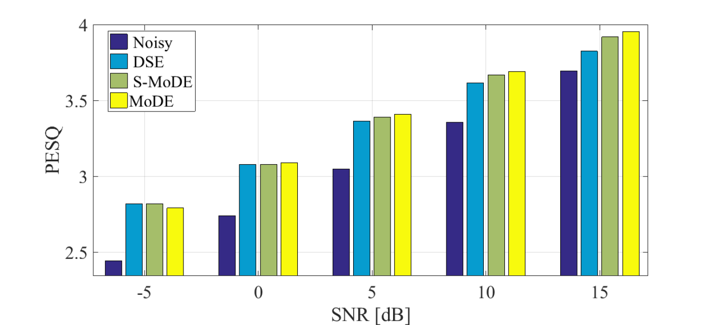
(a) Car noise

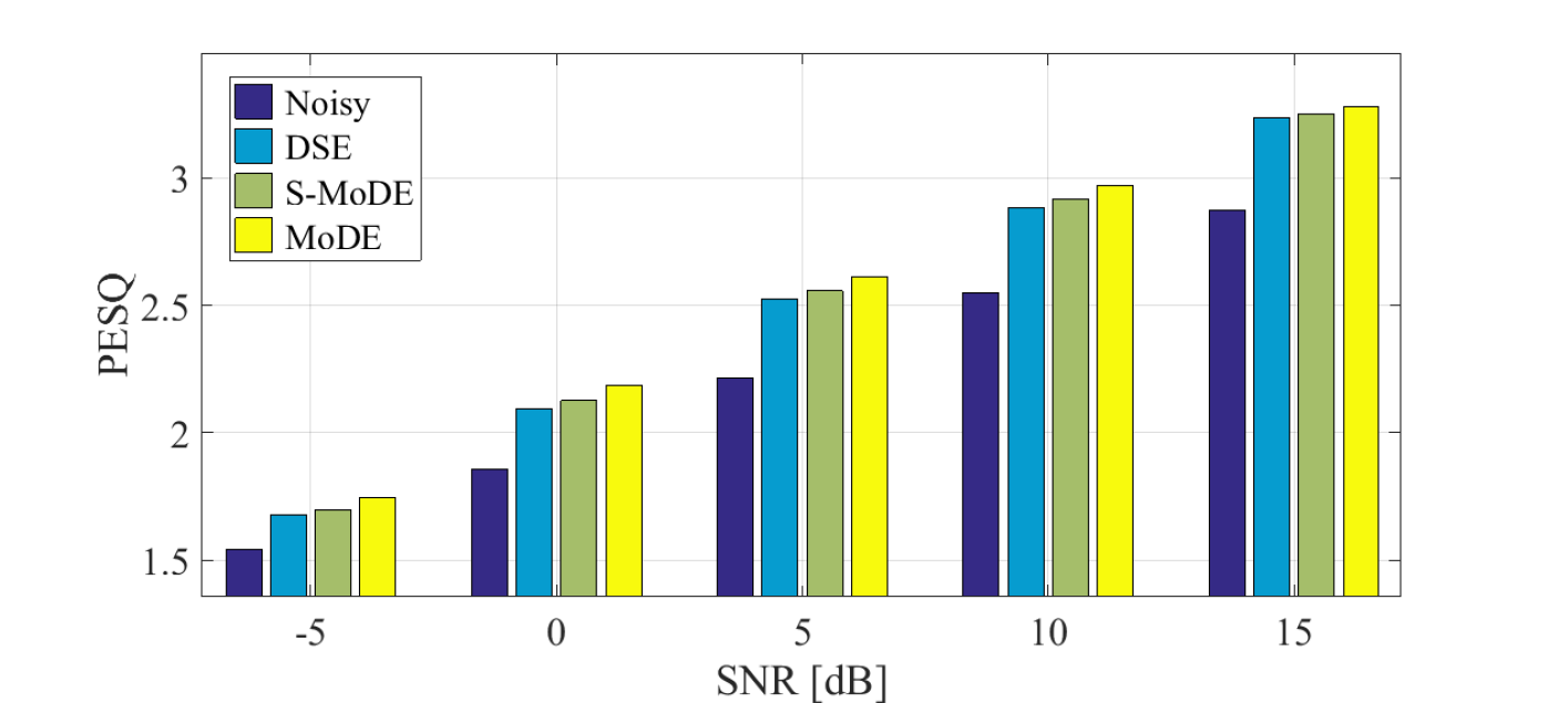
(b) Room noise

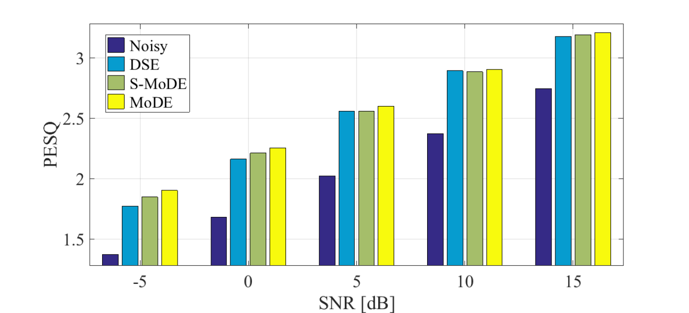
(c) Factory noise

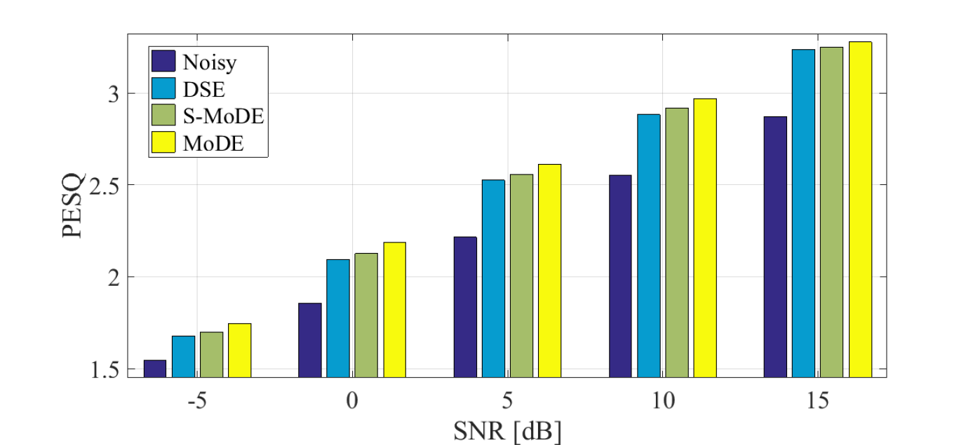
(d) Babble noise

Fig. 1: PESQ results on various noise types.

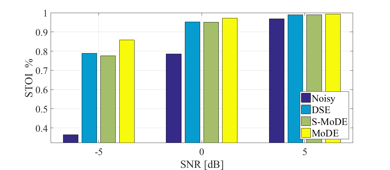
(a) Speech noise

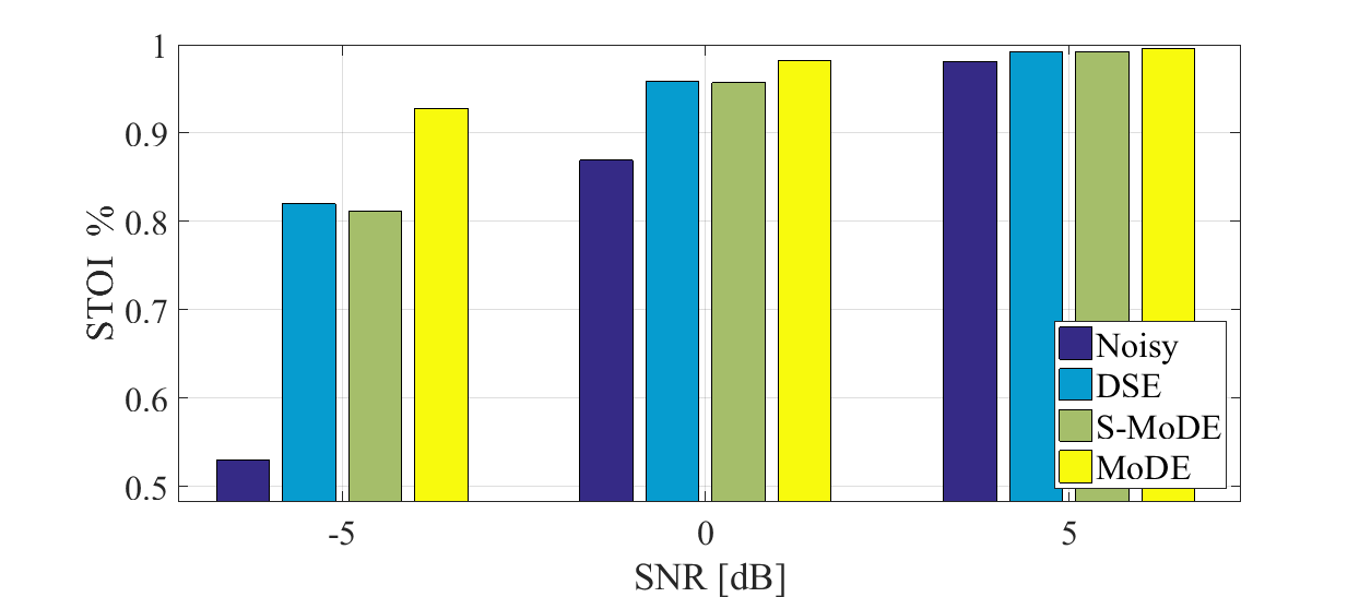
(b) Room noise

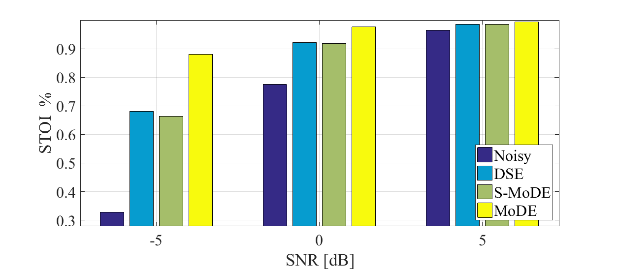
(c) Factory noise

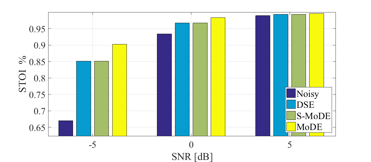
(d) White noise

Fig. 2: STOI results for several noise types.

Setup To test the proposed MoDE algorithm we contaminated the speech utterances with several types of noise from the NOISEX-92 database [21], namely Car, Room, Factory and Babble. The noise was added to the clean signal drawn from the test set of the TIMIT database (24-speaker core test set), with 5 levels of signal to noise ratio (SNR) at $-5$ dB, $0$ dB, $5$ dB, $10$ dB and $15$ dB chosen to represent various real-life scenarios.

Compared methods We compared the proposed MoDE algorithm with two DNN-based algorithms: 1) Deep single expert (DSE) is a fully-connected architecture that can be viewed as a single-expert network; and 2) S-MoDE is a supervised phoneme-based MoDE architecture [19]. The network has 39 experts where each expert is explicitly associated with a specific phoneme and training uses the phoneme labeling available in the TIMIT dataset.

When using the MoDE algorithm we need to set the number of experts. In most MoE studies, the number of experts was determined by an exhaustive search [22]. We found that increasing the number of experts from one to five significantly improves the performance and that additional experts had little effect. Hence, we chose the simpler model and set $m=5$. Each expert component in the S-MoDE network has the same network architecture as the expert block of the proposed MoDE model. The deep single expert (DSE) architecture is a single DNN chosen to have the same size (in terms of the total number of neurons in each hidden layer) of the MoDE with 5 experts, for fair comparison.

Training Procedure All the compared DNN-based algorithms were trained with the same database. We used the TIMIT database [23] train set (contains 462 speakers with 3.14 hours) for the training phase and the test set (containing 168 speakers with 0.81 hours) for the test phase. Note, that the train and test sets of TIMIT do not overlap. Clean utterances were contaminated by multiple noise types, stationary and non-stationary, with varying SNRs. The speech diversity modeling provided by the expert set was found to be rich enough to handle noise types that were not presented in the training phase.

The inputs to all DNN-based algorithms are the log-spectra vector and its corresponding MFCC vector. The log-spectra and the MFCC vectors were concatenated to form the input feature vector of the DSE network. In the case of MoDE, log-spectra were used as the input of the expert network and MFCC coefficients were the input of the gating network. Additionally, all methods apply the same enhancement scheme using (3), where we set $\beta$ to correspond to attenuation of $20$ dB, a value which yielded high noise suppression while maintaining low speech distortion.

The network was implemented in tensorflow [24] with ADAM optimizer [25] and batch-normalization was applied to each layer [26]. To overcome the mismatch between the training and the test conditions, each utterance was normalized prior to the training of the network, such that the sample-mean and sample-variance of the utterance were zero and one, respectively [27]. In order to circumvent over-fitting of the DNNs to the training database, we first applied the cepstral mean and variance normalization (CMVN) procedure to the input, prior to the training and test phases [27].

Objective quality measure results To evaluate the performance of the proposed speech enhancement algorithm, the standard perceptual evaluation of speech quality (PESQ) measure, which is known to have a high correlation with subjective score [28], was used. Intelligibility improvement was also evaluated using STOI [29]. We also carried out informal listening tests with approximately thirty listeners.

Figure 1 depicts the PESQ results of all algorithms for the Car, Room, Factory and Babble noise types as a function of the input SNR. Figure 2 depicts the STOI results for the same experiment setup. It is evident that both MoDE and S-MoDE, which split the noisy speech enhancement task into simpler problems, outperform the fully-connected network DSE. Moreover, the proposed method, MoDE, even outperforms the supervised method, S-MoDE, which exploits the phoneme information. This indicates that splitting the noisy data according to the phonemes is not an optimal strategy for enhancement and allowing the network to find by itself a suitable splitting of the data yields improved results.

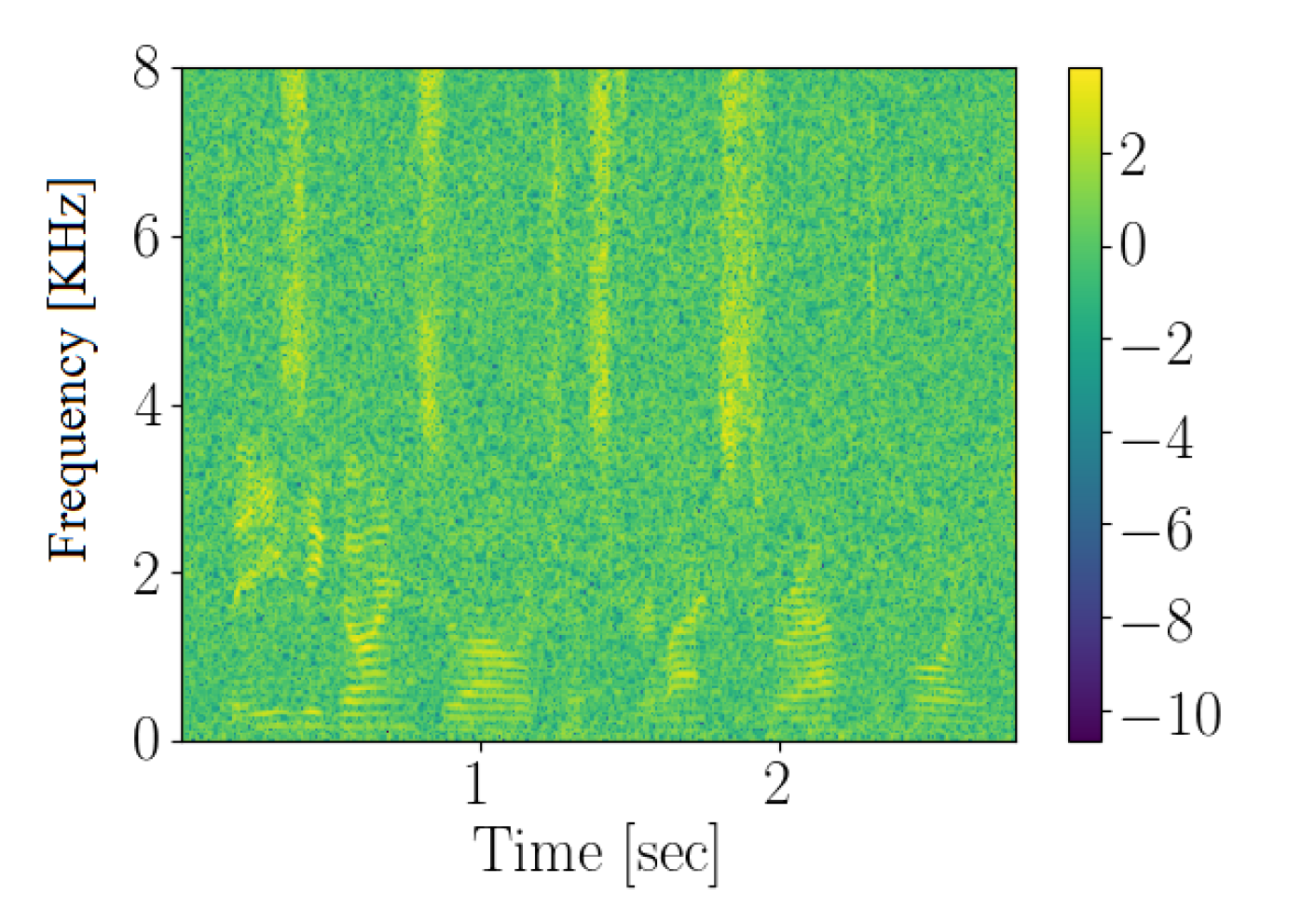
(a) Noisy input.

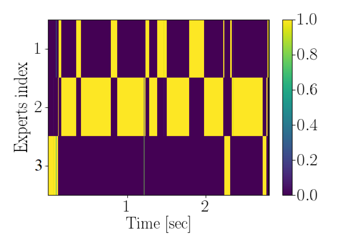
(b) Gate output, $\hat{\mathbf{p}}=[\hat{p}_{1},\hat{p}_{2},\hat{p}_{3}]$.

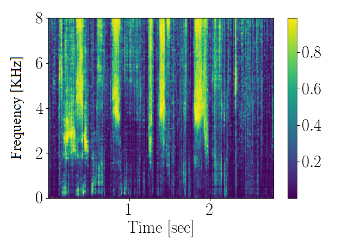
(c) Expert 1 mask estimation, $\hat{\boldsymbol{\rho}}_{1}$.

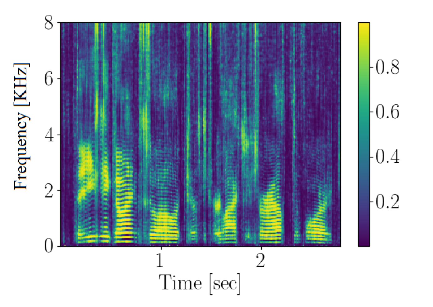
(d) Expert 2 mask estimation, $\hat{\boldsymbol{\rho}}_{2}$.

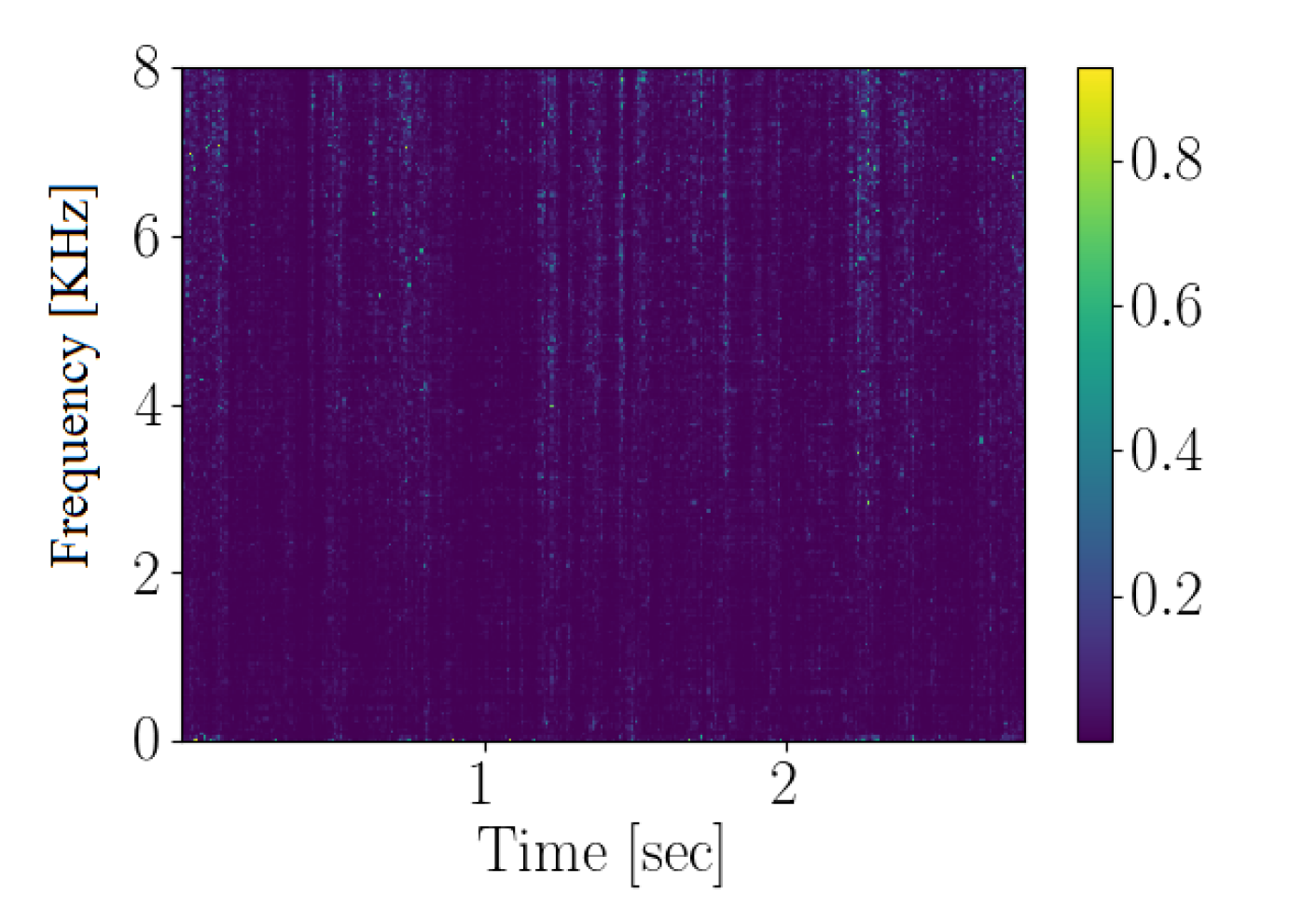
(e) Expert 3 mask estimation, $\hat{\boldsymbol{\rho}}_{3}$.

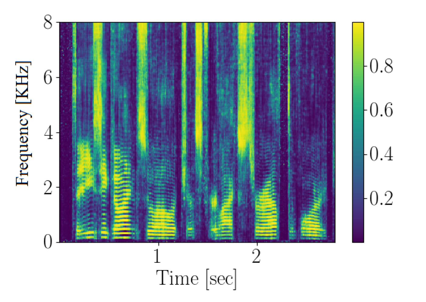
(f) Final estimation, $\hat{\boldsymbol{\rho}}=\sum_{i=1}^{3}\hat{p}_{i}\cdot\hat{\boldsymbol{\rho}}_{i}$.

Fig. 3: Experts and gate outputs of network with 3 experts.

Interpretation of the learned experts To gain a deeper understanding of the role of different experts, we next present for each expert $i$ the mask estimation $\hat{\rho}_{i}$ for an example of noisy speech utterance contaminated by white noise SNR=5 dB (Fig. 3(a)). Additionally, we show the distribution of the decisions of the gate DNN along the time.

In this case, the gate network classifies the noisy speech into three classes, voiced frames, unvoiced frames and speech inactive frames (Fig. 3(b)). We can see that the expertise of the first expert is to enhance the unvoiced parts of the speech (Fig. 3(c)), while the second expert is responsible for the voiced parts of the speech (Fig. 3(d)). Both experts do not perform well when the opposite speech pattern is introduced. The third expert expertise is to estimate the mask when only noise is present (Fig. 3(e)). The final weighted average masking decision is shown in Fig. 3(f).

We can also deduce from the gate decisions in Fig. 3(b) that for each time-frame the gate DNN tends to select only one expert. Consequently, each speech pattern is treated differently. Unlike the DSE DNN, in which a single network has to deal with the high variability of the speech patterns, our proposed method splits the speech enhancement task into $m$ simpler tasks, and therefore outperforms the competing DSE.

This experiment suggests that each expert is responsible for a specific pattern of the speech spectrum. Consequently, the experts preserve the speech structure and a more robust behavior is exhibited compared to other DSE-based algorithm. The S-MoDE do preserves the phoneme structures with supervised learning. Yet, is seems that the unsupervised classification of the speech patterns is more beneficial.

As a byproduct, we also gain complexity reduction at test time. For each time frame the gate first outputs a probabilities vector. The expert with the highest probability is therefore, $i^{\prime}=\operatornamewithlimits{argmax}_{i}\{\hat{p}_{i}\}$. Consequently, we can use only one expert for each time frame,

$$\hat{\boldsymbol{\rho}}=\sum_{i=1}^{m}\hat{p}_{i}\cdot\hat{\boldsymbol{\rho}}_{i}\approx\hat{\boldsymbol{\rho}}_{i^{\prime}}.$$ (10)

Therefore, even with larger number of experts, $m$, the same complexity of the gate and one of the expert is preserved.

5 Conclusion

This study introduced a MoDE model for speech enhancement. This approach splits the challenging task of speech enhancement into subspaces, where each DNN expert is responsible for a simpler task which corresponds to a different speech type. The gating DNN weights the outputs of the experts. This approach makes it possible to alleviate the well-known problem of DNN-based algorithms, namely, the mismatch between training phase and test phase. Additionally, the proposed MoDE architecture enables training with a small database of noises and as a by product also reduce the complexity at test time. The experiments verified that the proposed algorithm outperforms other DNN-based approaches in both objective and subjective measures.

References

- [1] P. C. Loizou, Speech enhancement: theory and practice, CRC press, 2013.
- [2] I. Cohen and B. Berdugo, “Speech enhancement for non-stationary noise environments,” Signal processing, vol. 81, no. 11, pp. 2403–2418, 2001.
- [3] I. Cohen and B. Berdugo, “Noise estimation by minima controlled recursive averaging for robust speech enhancement,” IEEE Signal Processing Letters, vol. 9, no. 1, pp. 12–15, 2002.
- [4] D. Wang and J. Chen, “Supervised speech separation based on deep learning: An overview,” IEEE/ACM Transactions on Audio, Speech, and Language Processing, vol. 26, no. 10, pp. 1702–1726, 2018.
- [5] A. Defossez, G. Synnaeve, and Y. Adi, “Real time speech enhancement in the waveform domain,” arXiv preprint arXiv:2006.12847, 2020.
- [6] J. Lee, Y. Jung, M. Jung, and H. Kim, “Dynamic noise embedding: Noise aware training and adaptation for speech enhancement,” arXiv preprint arXiv:2008.11920, 2020.
- [7] M. Kolbæk, Z.-H. Tan, S. H. Jensen, and J. Jensen, “On loss functions for supervised monaural time-domain speech enhancement,” IEEE/ACM Transactions on Audio, Speech, and Language Processing, vol. 28, pp. 825–838, 2020.
- [8] T. Lan, Y. Lyu, W. Ye, G. Hui, Z. Xu, and Q. Liu, “Combining multi-perspective attention mechanism with convolutional networks for monaural speech enhancement,” IEEE Access, vol. 8, pp. 78979–78991, 2020.
- [9] Y. Wang, J. Chen, and D. Wang, “Deep neural network based supervised speech segregation generalizes to novel noises through large-scale training,” Dept. of Comput. Sci. and Eng., The Ohio State Univ., Columbus, OH, USA, Tech. Rep. OSU-CISRC-3/15-TR02, 2015.
- [10] A. Das and J. H.L. Hansen, “Phoneme selective speech enhancement using parametric estimators and the mixture maximum model: A unifying approach,” IEEE Transactions on Audio, Speech, and Language Processing, vol. 20, no. 8, pp. 2265–2279, 2012.
- [11] S. E. Chazan, J. Goldberger, and S. Gannot, “A hybrid approach for speech enhancement using MoG model and neural network phoneme classifier,” IEEE/ACM Transactions on Audio, Speech, and Language Processing, vol. 24, no. 12, pp. 2516–2530, 2016.
- [12] Z. Q. Wang, Y. Zhao, and D. Wang, “Phoneme-specific speech separation,” in IEEE International Conference on Acoustics, Speech and Signal Processing (ICASSP), 2016.
- [13] Y. Wang, A. Narayanan, and D. Wang, “On training targets for supervised speech separation,” IEEE Transactions on Audio, Speech, and Language Processing, vol. 22, no. 12, pp. 1849–1858, 2014.
- [14] S. Boll, “Suppression of acoustic noise in speech using spectral subtraction,” IEEE Transactions on Acoustics, Speech and Signal Processing, vol. 27, no. 2, pp. 113–120, 1979.
- [15] O. Cappé, “Elimination of the musical noise phenomenon with the Ephraim and Malah noise suppressor,” IEEE Transactions on Speech and Audio Processing, vol. 2, no. 2, pp. 345–349, 1994.
- [16] R. A Jacobs, M. I. Jordan, S. J Nowlan, and G. E. Hinton, “Adaptive mixtures of local experts,” Neural computation, vol. 3, no. 1, pp. 79–87, 1991.
- [17] M. I. Jordan and R. A. Jacobs, “Hierarchical mixtures of experts and the EM algorithm,” Neural computation, vol. 6, no. 2, pp. 181–214, 1994.
- [18] H. Hermansky, J. R. Cohen, and R. M. Stern, “Perceptual properties of current speech recognition technology,” Proceedings of the IEEE, vol. 101, no. 9, pp. 1968–1985, 2013.
- [19] S. E. Chazan, S. Gannot, and J. Goldberger, “A phoneme-based pre-training approach for deep neural network with application to speech enhancement,” in International Workshop on Acoustic Signal Enhancement (IWAENC), 2016.
- [20] J. Xie, R. Girshick, and A. Farhad, “Unsupervised deep embedding for clustering analysis,” in International Conference on Machine Learning (ICML), 2016.
- [21] A. Varga and H. J.M. Steeneken, “Assessment for automatic speech recognition: NOISEX-92: A database and an experiment to study the effect of additive noise on speech recognition systems,” Speech communication, vol. 12, no. 3, pp. 247–251, 1993.
- [22] D. E. Yuksel, J. N. Wilson, and P. D. Gader, “Twenty years of mixture of experts,” IEEE Transactions on Neural Networks and Learning Systems, vol. 23, no. 8, pp. 1177–1193, 2012.
- [23] J. S. Garofalo, L. F. Lamel, W. M. Fisher, J. G. Fiscus, D. S. Pallett, and N. L. Dahlgren, “The DARPA TIMIT acoustic-phonetic continuous speech corpus CD-ROM,” Tech. Rep., Linguistic Data Consortium, 1993.
- [24] M. Abadi, P. Barham, J. Chen, Z. Chen, A. Davis, J. Dean, M. Devin, S. Ghemawat, G. Irving, M. Isard, et al., “Tensorflow: a system for large-scale machine learning.,” in OSDI, 2016, vol. 16, pp. 265–283.
- [25] D. Kingma and J. Ba, “ADAM: A method for stochastic optimization,” arXiv preprint arXiv:1412.6980, 2014.
- [26] S. Ioffe and C. Szegedy, “Batch normalization: Accelerating deep network training by reducing internal covariate shift,” in International Conference on Machine Learning (ICML), 2015.
- [27] J. Li, L. Deng, Y. Gong, and R. Haeb-Umbach, “An overview of noise-robust automatic speech recognition,” IEEE Transactions on Audio, Speech, and Language Processing, vol. 22, no. 4, Apr. 2014.
- [28] P Recommendation, “862: Perceptual evaluation of speech quality (PESQ): An objective method for end-to-end speech quality assessment of narrow-band telephone networks and speech codecs,” Feb., vol. 14, 2001.
- [29] C. H. Taal, R. C. Hendriks, R. Heusdens, and J. Jensen, “An algorithm for intelligibility prediction of time–frequency weighted noisy speech,” IEEE Transactions on Audio, Speech, and Language Processing, vol. 19, no. 7, pp. 2125–2136, 2011.