Dynamical orbital evolution scenarios of the wide-orbit eccentric planet HR 5183b

Abstract

The recently-discovered giant exoplanet HR5183b exists on a wide, highly-eccentric orbit ($a=18$ au, $e=0.84$). Its host star possesses a common proper-motion companion which is likely on a bound orbit. In this paper, we explore scenarios for the excitation of the eccentricity of the planet in binary systems such as this, considering planet–planet scattering, Lidov–Kozai cycles from the binary acting on a single-planet system, or Lidov–Kozai cycles acting on a two-planet system that also undergoes scattering. Planet–planet scattering, in the absence of a binary companion, has a $2.8-7.2\%$ probability of pumping eccentricities to the observed values in our simulations, depending on the relative masses of the two planets. Lidov–Kozai cycles from the binary acting on an initially circular orbit can excite eccentricities to the observed value, but require very specific orbital configurations for the binary and overall there is a low probability of catching the orbit at the high observed high eccentricity ($0.6\%$). The best case is provided by planet–planet scattering in the presence of a binary companion: here, the scattering provides the surviving planet with an initial eccentricity boost that is subsequently further increased by Kozai cycles from the binary. We find a success rate of $14.5\%$ for currently observing $e\geq 0.84$ in this set-up. The single-planet plus binary and two-planet plus binary cases are potentially distinguishable if the mutual inclination of the binary and the planet can be measured, as the latter permits a broader range of mutual inclinations. The combination of scattering and Lidov–Kozai forcing may also be at work in other wide-orbit eccentric giant planets, which have a high rate of stellar binary companions.

1 Introduction

The G0 star HR 5183 ($M_{\star}=1.07\pm 0.04\mathrm{\,M}_{\odot}$), has been found to host a super-Jovian planet ($M\sin I=3.23^{+0.58}_{-0.55}\mathrm{\,M_{J}}$) on a highly-eccentric orbit (Blunt et al., 2019). While the orbit of the planet is wide and its semimajor axis poorly constrained ($a=18^{+6}_{-4}$ au), good coverage of the planet’s periastron passage both permitted its discovery and provided a good determination of the orbital eccentricity ($e=0.84\pm 0.04$).

The high eccentricity of HR 5183b suggests that significant changes to the planet’s orbit have happened in the past, as planets form on near-circular orbits. Planet–planet scattering has been shown to be able to produce high eccentricities (Rasio & Ford, 1996; Weidenschilling & Marzari, 1996; Chatterjee et al., 2008; Jurić & Tremaine, 2008). The eccentricity distribution of giant planets implies that around 80% of them formed in unstable multi-planet systems (Jurić & Tremaine, 2008; Raymond et al., 2011). Planet–planet scattering can excite eccentricity even to near-unity values (Carrera et al., 2019); and the more massive the planet ejected, the larger the eccentricity of the survivor (e.g., Kokaia et al., 2020, figure 1). Thus, the high eccentricity of HR 5183b would suggest that it formed in a system with at least one other super-Jovian planet, of which it is the only survivor.

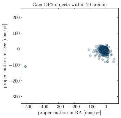
Figure 1: Proper motions of all objects in Gaia DR2 within 20 arcmin of HR 5183. HR 5183 and HIP 67291 are the two barely-distinguishable points at around $(-500,-100)$. Their remoteness from the main cloud of field objects means that the probablility that the pair is a chance alignment of unbound objects is vanishingly small.

However, HR 5183 possesses a common-proper motion companion (Allen et al., 2000). Figure 1 shows the proper motions of all objects within 20 arcmin of HR 5183 from Gaia DR2 (Gaia Collaboration et al., 2016, 2018), underlining the extremely low likelihood that this is a chance alignment. Furthermore, the parallax and radial velocity of the two stars are almost identical (Blunt et al., 2019). This star, of mass $M=0.67\pm 0.05\mathrm{\,M}_{\odot}$, has a projected separation of 15 000 au. The high-quality astrometric data from Gaia allowed Blunt et al. (2019) to constrain the orbital elements of the binary: the distribution of semi-major axis and eccentricity (for bound orbits) is shown in the left-hand panel of Figure 2. Details of the HR 5183 system are given in Table 1. While too distant to affect the protoplanetary disc where planet formation takes place (Harris et al., 2012), the presence of a binary companion would complicate the subsequent planet–planet scattering described above: it could trigger an instability in an otherwise stable system, and/or it could affect the orbit of a planet that survives the scattering process.

Table 1: Relevant parameters for the HR 5183 system from Blunt et al. (2019), together with values adopted for the simulations.

Parameter	Blunt et al. (2019) value	Adopted value
Primary mass $M_{\star}$	$1.07^{+0.04}_{-0.04}\mathrm{\,M}_{\odot}$	$1.07\mathrm{\,M}_{\odot}$
System age $t_{\mathrm{age}}$	$7.7^{+1.4}_{-1.2}$ Gyr	$8$ Gyr
Secondary mass $M_{\mathrm{B}}$	$0.67^{+0.05}_{-0.05}\mathrm{\,M}_{\odot}$	$0.67\mathrm{\,M}_{\odot}$
Binary semimajor axis1 $a_{\mathrm{B}}$	see Figure 2	drawn from
Binary eccentricity1 $e_{\mathrm{B}}$	see Figure 2	joint posterior
Planet minimum mass $M_{\mathrm{b}}\sin I$	$3.23^{+0.15}_{-0.14}\mathrm{\,M_{J}}$	$M_{\mathrm{b}}=3.23\mathrm{\,M_{J}}$
Planet semimajor axis $a_{\mathrm{b}}$	$18^{+6}_{-4}$ au	$18$ au
Planet eccentricity $e_{\mathrm{b}}$	$0.84\pm 0.04$	$0.84$
1 restricting to bound orbits $<200\,000$ au.

Wide binary companions can excite an exoplanet’s eccentricity from an initial low value through Lidov–Kozai cycles, if the binary’s orbital inclination is sufficiently high (Kozai, 1962; Lidov, 1962). However, the higher the eccentricity one wishes to attain, the higher the initial inclination required; furthermore, planets only spend a short time at the peak of the eccentricity cycle. As we show below, these factors mean that it is unlikely that we are observing the planet at its present high eccentricity if the dynamics responsible were purely Lidov–Kozai excitation from a near-circular initial orbit.

In this Paper, we therefore consider the two effects, of planet–planet scattering and Lidov–Kozai cycles from a binary companion, operating in concert. In otherwise stable multi-planet systems, planet–planet interactions can suppress the Lidov–Kozai cycles (Innanen et al., 1997; Malmberg et al., 2007; Kaib et al., 2011; Boué & Fabrycky, 2014; Mustill et al., 2017; Pu & Lai, 2018; Denham et al., 2019); alternatively, the binary companion can destabilise the planetary system by inducing a large eccentricity on the outermost planet (Malmberg et al., 2007; Mustill et al., 2017). The binary destabilises the system if the timescale for Lidov–Kozai cycles is shorter than that for secular planet–planet interactions. On the other hand, a multi-planet system may be closely spaced enough to undergo an internal instability, without external triggering (Gladman, 1993; Chambers et al., 1996; Quillen, 2011; Petit et al., 2020). In this case, the binary companion can subsequently further excite the eccentricity of a planet that survives the instability (Kaib et al., 2013). We show in this paper that this significantly increases the probability of observing a planet at a high eccentricity, above either planet–planet scattering alone or Lidov–Kozai cycles alone.

This paper is organised as follows: in Section 2 we describe the set-up of our three sets of $N$-body simulations; in Section 3 we present the outcomes of the simulations; and in Section 4 we discuss the results. We conclude in Section 5.

2 Simulation set-up

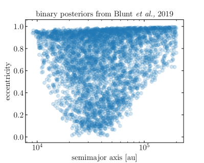
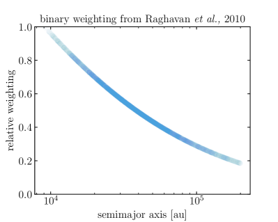
Figure 2: Left: Binary orbital parameters from Blunt et al. (2019). 3 936 draws from the posterior distribution are shown, restricted to bound orbits with semimajor axis less than 200 000 au. These orbits are then sampled to draw the binary companions for the $N$-body simulations. Right: Weighting applied when sampling from the binary orbits from Blunt et al. (2019) in the weighted runs; the weighting is from the observed lognormal binary period distribution of Raghavan et al. (2010).

We conduct several sets of $N$-body simulations to explore the origin of the high eccentricity of HR 5183b. The simulations were all run with Mercury (Chambers, 1999) using the accurate RADAU integrator (Everhart, 1985), with an error tolerance of $10^{-11}$. We adopted the values $M_{\star}=1.07\mathrm{\,M}_{\odot}$ and $R_{\star}=1.53\mathrm{\,R}_{\odot}$ from Blunt et al. (2019). Collisions between planets, or between a planet and a star, are treated as perfect inelastic mergers.

We run three sets of simulations: pure scattering, with the primary star and two planets; pure Kozai, with the primary star, one planet, and the binary companion; and combined scattering and Kozai, with the primary star, two planets and the binary companion:

1. Pure scattering: Here we consider the simplest case of planet–planet scattering, and set up systems each with two planets. One set of runs has equal planet masses $M_{1}=M_{2}=3.23\mathrm{\,M_{J}}$, and three sets have planet–planet mass ratios $\mu=1.2$, $1.5$ and $2.0$, where the smaller planet has mass $M_{1}=3.23\mathrm{\,M_{J}}$. The inner planet is placed at $a_{1}=36\mathrm{\,au}$; this means that its semimajor axis shrinks to roughly the observed $18$ au after ejection of the comparable-mass outer planet. The exact final semimajor axis is not significant, because at these separations with very rare physical collisions the dynamics is essentially scale-invariant. The outer planet itself is placed at $a_{2}\in a_{1}\times[1,1+3.6((M_{1}+M_{2})/M_{\star})^{1/3}]$, thus extending beyond the Hill stability boundary (Gladman, 1993) in order to include systems which are Hill stable but Lagrange unstable (Veras & Mustill, 2013). In the unequal-mass cases the more massive planet is exterior to encourage its ejection and help the surviving planet attain a higher eccentricity. Planets are started on circular orbits with a small mutual inclination of up to $1^{\circ}$. Systems are integrated for 1 Gyr (most instabilities occur early, and very few at such late times) or until the loss of a planet by collision or ejection from the system. Thus these systems extend to several 10s of au; while rare, direct imaging surveys show that systems of multiple giant planets at these orbital radii and beyond do indeed exist (e.g., Marois et al., 2008; Bohn et al., 2020).

2. Pure Kozai: Here we place one planet at 18 au and add a binary stellar companion drawn from the posterior orbit fits of Blunt et al. (2019, see below). The binary orbit is oriented isotropically with respect to that of the planet (while we have constraints on the present binary orbital inclination, we are at this stage agnostic as to the initial orbital inclination of the planet). The binary star’s mass is $0.67\mathrm{\,M}_{\odot}$. Systems are integrated for the system age of 8 Gyr.

3. Combined scattering and Kozai: here we place two near-coplanar equal-mass planets in each system, as in the pure scattering runs, and add a binary stellar companion as in the Kozai runs. Systems are again integrated for the system age of 8 Gyr. We note that in principle the addition of the binary companion could act to destabilise the planetary system as Lidov–Kozai cycles could be induced on the outermost planet, making scattering more likely (Innanen et al., 1997; Malmberg et al., 2007; Pu & Lai, 2018; Denham et al., 2019). However, the binary companions in our systems are too widely spaced: the timescale for Lidov–Kozai interactions is typically $\gtrsim 1$ Gyr, and these are therefore suppressed by planet–planet interactions which have timescales $\lesssim 1$ Myr. These combined systems therefore evolve first under planet–planet scattering, and then under Lidov–Kozai perturbations from the companion.

For the runs with binaries, we run both Unweighted and Weighted sets. In the Unweighted runs we draw the binary semimajor axis and eccentricity from the posterior distributions of Blunt et al. (2019), restricting ourselves to bound orbits with semimajor axes $<200\,000$ au ($\sim 1$ pc, taken as a crude upper limit of where a binary would avoid being broken up in the Galactic field); draws from this distribution are shown in the left-hand panel of Figure 2. These posteriors derive from the reported formal errors in Gaia DR2, not accounting for possible systematics. These posterior distributions also had a uniform prior on the binary semimajor axis distribution. However, the period distribution of the binary population for Solar-type stars appears to be lognormal with a mean of $\log(P/\mathrm{d})=5.03$ and a standard deviation of $\sigma_{\log P/\mathrm{d}}=2.28$ (Raghavan et al., 2010); Tokovinin & Lépine (2012) show that this distribution extends to the very wide binaries beyond $\sim 10\,000$ au that we consider here. We therefore construct Weighted sets of simulations where the posterior from Blunt et al. (2019) is weighted by the binary semimajor axis with the lognormal weighting function shown in the right-hand panel of Figure 2.

3 Results

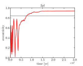
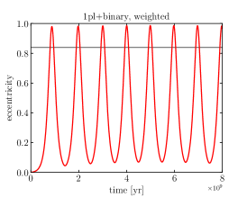
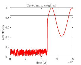
Figure 3: Examples of eccentricity evolution for the surviving planet in three runs where $e>0.84$ at the end of the simulation. Left: Two planets with no binary companion. After an initial phase of scattering the second planet is ejected at 25 Myr, freezing in the surviving planet’s eccentricity at a high value. Centre: Single planet with binary companion. The planet’s eccentricity cycles up and down under the influence of Lidov–Kozai perturbations. We are fortunate enough to catch the system in a high-eccentricity phase at the end of the simulation. Right: Two planets with a binary companion. After scattering ust before 5 Gyr, the surviving planet undergoes Lidov–Kozai oscillations imposed by the binary. While a favourable phase is still required to observe the planet at a high eccentricity at the epoch of observation, note that the ecentricity is greater than that observed over a much greater fraction of the cycle than in the case of the single planet plus companion. In each panel, we mark the target eccentricity of $0.84$ with a horizontal grey line.

First, we define for all simulations our success criterion: the existence of a planet at an eccentricity greater than or equal to that observed at the end of the simulation: $e_{\mathrm{final}}\geq 0.84$. When calculating fractions of successful runs in the simulations containing two planets, we only count systems which actually underwent an instability. This avoids our having to test different distributions of initial orbital spacing, by which we could make the fraction of unstable systems arbitrarily large or small. We choose not to impose a semi-major axis cut on the surviving planets for two reasons. Firstly, at these distances from the star, collisions between bodies are extremely unlikely, and so a system undergoing scattering can be rescaled to match a given semimajor axis. Second, we lack a predictive theory of planet formation, and observations are not as yet very constraining about the planet population at tens of au, so it is hard to know what initial conditions in semimajor axis should be. However, it is much more certain that planets form on low-eccentricity orbits, and hence the current eccentricity provides the strongest useful constraint on the system’s dynamical history.

3.1 Pure scattering

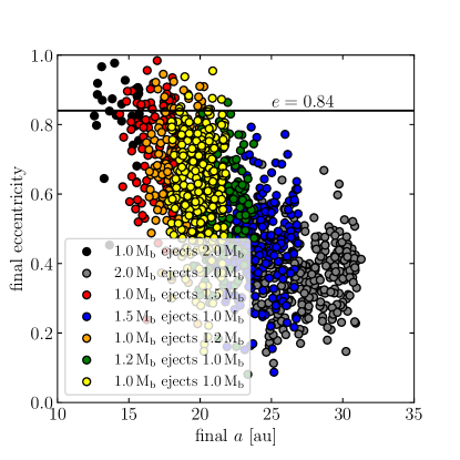
Figure 4: Orbital elements of the surviving planet after instability in unstable two-planet systems with no binary companion. Different colours indicate different ratios of ejected to retained planet mass. The black horizontal line marks the target eccentricity, $e=0.84$.

Table 2: Results of the two-planet runs, with no binary companion. We show the mass ratio of the two planets, the number of simulations $n_{\mathrm{runs}}$; the number that were unstable $n_{\mathrm{unstable}}$; the number where the surviving planet had an eccentricity above $0.84$ at the end of the simulation $n_{e\geq 0.84}$; and the success fraction $f_{\mathrm{success}}=n_{e\geq 0.84}/n_{\mathrm{unstable}}$.

Simulation set	$m_{\mathrm{out}}/m_{\mathrm{in}}$	$n_{\mathrm{runs}}$	$n_{\mathrm{unstable}}$	$n_{e\geq 0.84}$	$f_{\mathrm{success}}$
2pl-mu1.0	1.0	4991	324	9	2.8%
2pl-mu1.2	1.2	500	359	19	5.3%
2pl-mu1.5	1.5	500	376	27	7.2%
2pl-mu2.0	2.0	500	370	14	3.8%
1 One run with bad energy conservation was removed ($|\mathrm{d}E/E|>10^{-3}$). Other typical energy errors were $\sim 10^{-5}$ or less for this simulation set, and much lower for the other sets.

Our two-planet systems are initially tightly packed, resulting in most of them ($65-75\%$) being unstable (see Table 2). If a system is unstable, the most common outcome is the ejection of one planet, usually the least massive. Physical collisions between the planets are rare because of the small physical radius compared to the large orbital radius. These planet–planet collisions invariably result in moderately low eccentricities of below $0.2$.

We show an example of the eccentricity evolution of a planet that attains the target eccentricity in the left-hand panel of Figure 3. The system rapidly becomes unstable and the second planet is ejected at $~{}\sim 25$ Myr. At this point, the surviving planet’s eccentricity, which has been excited to above $0.9$ by the scattering, is frozen at this high value and remains unchanged for the rest of the system’s history, as the origin of the sole perturbing force has been removed.

The orbital elements of the surviving planets following an ejection are shown in Figure 4. A planet ejects a body of similar mass and initial orbital radius, so its semimajor axis roughly halves to conserve energy, ending at around 18 au. Eccentricities are moderate to high, but few are at the observed value or higher, with success rates for $e\geq 0.84$ between 3 and 7% (Table 2). The eccentricity distribution is higher the more massive is the ejected planet, but ejection of a more massive planet is decreasingly unlikely with increasing mass. These tendencies work against each other and the most successful mass ratio is $1.5$ (Table 2). A Sankey diagram showing how different outcomes are obtained for this mass ratio is shown in Figure 5 (top panel). We see that although loss of the less massive planet is the dominant outcome of instability, all but one of the highly-eccentric planets are actually from systems where the more massive planet was ejected. The exception comes from one case where the less massive planet collided with the star, leaving the more massive survivor on a very wide orbit of several hundred au.

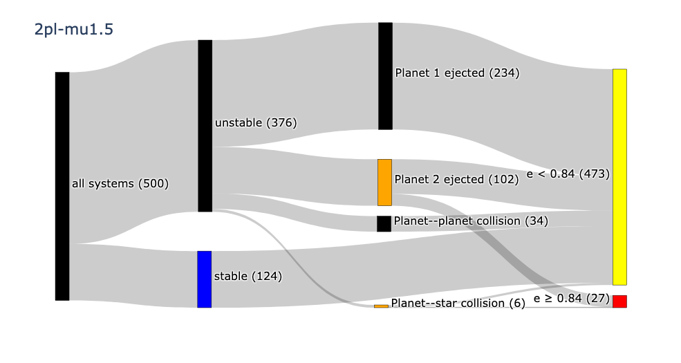
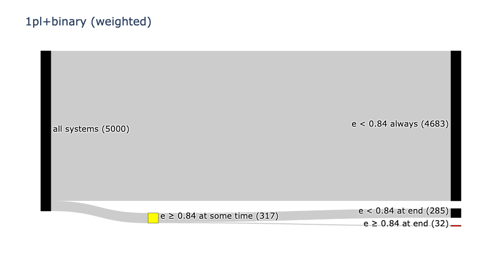
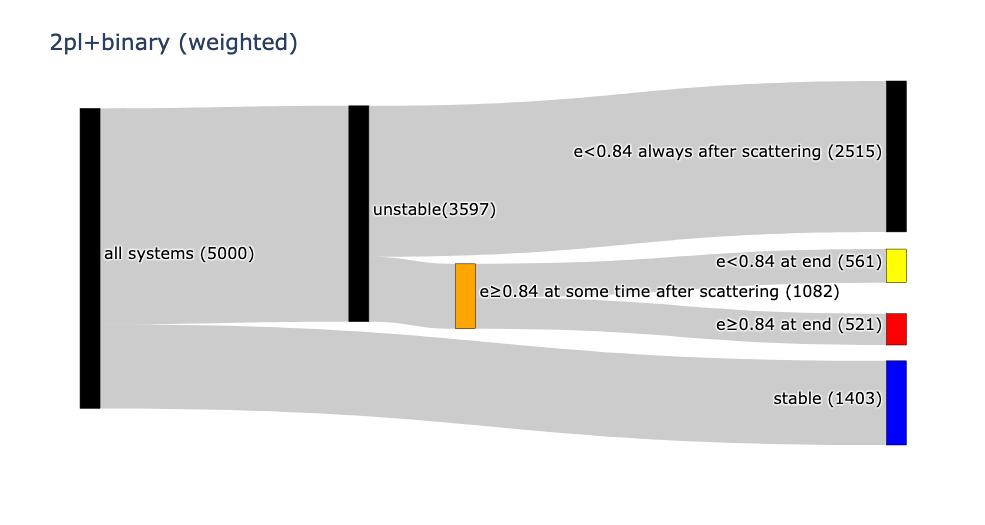
Figure 5: Simulation outcomes for our three scenarios. Top: Two-planet scattering simulations with no binary companion, for a planet–planet mass ratio of $\mu=m_{\mathrm{out}}/m_{\mathrm{in}}=1.5$ (the most favourable case for reaching the target eccentricity). Middle: Simulations with a single planet plus a binary companion drawn from the weighted posteriors of Blunt et al. (2019). Bottom: Simulations with a two equal-mass planets plus a binary companion drawn from the weighted posteriors of Blunt et al. (2019). Note the much larger fraction of systems with a planet at or above the target eccentricity in this case (red bar).

3.2 Pure Kozai

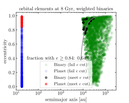
Figure 6: Orbital elements at 8 Gyr for the systems with a single planet, together with binary companions drawn from the weighted posteriors of Blunt et al. (2019). The grey line shows where the characteristic Kozai timescale (Equation 1) is $8$ Gyr. 5 000 simulations are run.

Table 3: Outcomes for the runs with one planet with a binary companion. For each simulation set we show the number of runs $n_{\mathrm{runs}}$; the number where the planet attained an eccentricity above $0.84$ at any point in the integration $n_{e\geq 0.84}$(ever); the number where the planet had an eccentricity greater than $0.84$ at the end of the simulation $n_{e\geq 0.84}$(8 Gyr); and the success fraction $f_{\mathrm{success}}=n_{e\geq 0.84}\textrm{(8\,Gyr)}/n_{\mathrm{runs}}$.

Simulation set	$n_{\mathrm{runs}}$	$n_{e\geq 0.84}$	$n_{e\geq 0.84}$	$f_{\mathrm{success}}$
		(ever)	(8 Gyr)
1pl+binary-unweighted	500	13	2	0.4%
1pl+binary-weighted	5000	317	32	0.6%

An example of one of our successful single-planet Kozai runs is shown in the centre panel of Figure 3. The highly-inclined ($81^{\circ}$) binary can excite eccentricities well above $0.9$ in the planetary orbit, and we are fortunate in this case to “observe” the system at 8 Gyr when it is at a high-eccentricity phase of the cycle. Note, however, that for most of the cycle the eccentricity is lower than the target value.

The presence of a sufficiently inclined binary companion induces oscillations in the planet’s eccentricity, with higher eccentricities being attained when the binary’s inclination is higher. In our simulations, $3-6\%$ of planets ever attain an eccentricity of $0.84$ or above (Table 3). As we have seen, however, and in contrast to the case of two-planet scattering (where orbital evolution ceases following the ejection of one planet), when the eccentricity excitation is due to a binary companion the planet’s orbit continues to evolve and the eccentricity can reduce from its peak. At the snapshot at 8 Gyr at the end of the simulations, only $0.4-0.6\%$ of planets have an eccentricity above $0.84$ (Table 3, Figure 6). That is, most planets which possess an eccentricity in the target range at some point do not do so at the end of the simulation: this is visualised in Figure 5 (middle panel). We see from the orbital elements presented in Figure 6 that it is only close and eccentric binary companions that can excite a high eccentricity within the system lifetime: the characteristic Kozai timescale is given by, e.g., Innanen et al. (1997)

$$t_{\mathrm{Koz}}=P_{\mathrm{b}}\left(\frac{a_{\mathrm{B}}}{a_{\mathrm{b}}}\right)^{3}\frac{M_{\mathrm{A}}}{M_{\mathrm{B}}}\left(1-e_{\mathrm{B}}^{2}\right)^{3/2},$$ (1)

where $P_{\mathrm{b}}$ is the planet’s orbital period. The locus where this estimated timescale is $8$ Gyr is shown in Figure 6.

The simulations we ran with the additional weighting on binary semimajor axis from Raghavan et al. (2010) were more successful than those without the additional weighting. This is because, with a higher fraction of closer binaries in these weighted runs, the distribution of Kozai timescales is shifted to shorter times.

3.3 Combined scattering and Kozai

Table 4: Outcomes for the runs with two planets with a binary companion. For each simulation set we show the number of runs $n_{\mathrm{runs}}$; the number where the planets underwent an orbital instability $n_{\mathrm{unstable}}$; the number where the planet attained an eccentricity above $0.84$ at any point in the integration $n_{e\geq 0.84}$(ever); the number where the planet had an eccentricity greater than $0.84$ at the end of the simulation $n_{e\geq 0.84}$(8 Gyr); and the success fraction $f_{\mathrm{success}}=n_{e\geq 0.84}\textrm{(ever)}/n_{\mathrm{runs}}$.

Simulation set	$n_{\mathrm{runs}}$	$n_{\mathrm{unstable}}$	$n_{e\geq 0.84}$	$n_{e\geq 0.84}$	$f_{\mathrm{success}}$
			(ever)	(8Gyr)
2pl+binary-unweighted	500	362	94	46	12.7%
2pl+binary-weighted	5000	3597	1082	521	14.5%

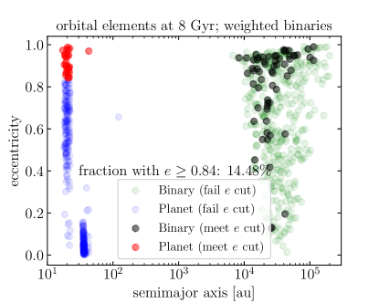
Figure 7: Orbital elements at 8 Gyr for the systems with two planets , together with a binary companions drawn from the weighted posteriors of Blunt et al. (2019). 500 out of 5 000 simulations run are shown.

We now study systems that initially comprise the primary star, two planets, and the binary companion. In these systems, Lidov–Kozai cycles can act to further modulate the surviving planet’s eccentricity after scattering; we see (Table 4) that this leads to significantly more planets having a high eccentricity at the end of the simulation than either scattering alone or binary perturbations alone.

An example of a successful system in this scenario is displayed in the right-hand panel of Figure 3. Here, the two planets undergo an instability, removing one planet and leaving the survivor with an eccentricity a little below the target value. This survivor then undergoes Lidov–Kozai perturbations imposed by the binary, periodically raising it eccentricity above the target value. While we still require a favourable epoch of observation to catch the planet at a high eccentricty, the eccentricity is above the target value for a much larger fraction of the cycle than in the case of the single planet excited from low eccentricity.

The semimajor axis and eccentricity of surviving planets and stars at 8 Gyr are shown in Figure 7. $10.4\%$ of all systems have a planet with $e\geq 0.84$, and $14.5\%$ of the unstable runs – an order of magnitude higher than the single-planet plus binary case, and also considerably higher than the equal-mass scattering with no binary companion. As in the case of the single planet plus binary, the binary companions in systems that reach $e\geq 0.84$ are preferentially on more eccentric orbits with smaller semimajor axes.

As seen in Figure 5 (bottom panel), now about half of the planets that ever have $e\geq 0.84$ (following scattering) still have $e\geq 0.84$ at 8 Gyr, a much higher fraction than in the single-planet Kozai case. We can understand both this and the higher fraction of planets that attain high eccentricities by referring to the phase portrait for Kozai cycles, as discussed in Section 4.

3.4 Relaxing the success criteria

We then repeated the calculations of success rates for a target eccentricity of $e=0.8$, $1\sigma$ below the observed value. This modestly increased the success rates of all runs: the single-planet weighted binaries had a success rate of $0.9\%$; the two-planet weighted binaries $19.5\%$; and the two-planet pure scattering rates of $6.8\%$, $8.9\%$, $11.2\%$ and $5.9\%$ for mass ratios $\mu=1$, $1.2$, $1.5$ and $2$ respectively. We also relaxed the eccentricity target to $0.672$ (20% below that observed), allowing us to account for the possibility of an underestimated formal error on the eccentricity measurement. Here, we found success rates of $1.8\%$ for single-planet weighted binaries, $41.7\%$ for two-planet weighted binaries, and $33.2\%$, $31.8\%$, $23.1\%$ and $9.2\%$ for two-planet scattering. On the whole, the combination of scattering and Lidov–Kozai perturbations remains the most effective.

Finally, we discuss relaxing the time constraint. While we consider the most useful definition of a success to be that the eccentricity is suitably high at a given epoch of observation, it is also worth exploring the fraction of systems that ever attain such a high eccentricity. For the single-planet weighted binary simulations, we find that 317 out of 5000 systems ever attain $e\geq 0.84$ (about 10 times the number at 8 Gyr), while for the two-planet weighted binary simulations, we find 1082 systems attain $e\geq 0.84$ (only about twice the number at 8 Gyr). The combination of scattering and Lidov–Kozai perturbations therefore increases the fraction of systems ataining high eccentricity at any time, but it also significantly increases the “duty cycle” at which these systems have high eccentricity, making them more likely to be observed in the high-eccentricity state.

4 Discussion

4.1 Why Kozai plus scattering works well

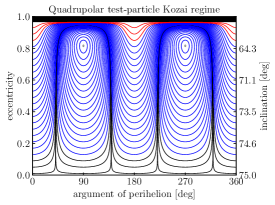
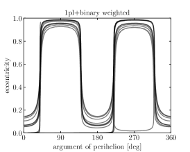
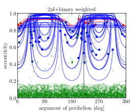
Figure 8: Left: phase portrait for the classical Lidov–Kozai resonance in the quadrupolar approximation with an interior test particle, with a constant $C_{\mathrm{Koz}}=\sqrt{1-e^{2}}\cos I=0.258806$. Eccentricity is plotted against the argument of pericentre ($\omega$, a measure of orbital orientation), and orbits evolve along the curves. The right-hand ordinate axis shows the value of inclination corresponding to the eccentricity on the left-hand axis. Black trajectories begin below $e=0.1$ and at some point attain $e\geq 0.84$; Blue trajectories begin between $e=0.1$ and $e=0.84$ and at some point attain $e\geq 0.84$; red trajectories are always above $e=0.84$; and grey trajectories (librating round the fixed points at $\omega=90^{\circ}$ and $270^{\circ}$) never attain $e\geq 0.84$. The black region at $e\approx 1$ is forbidden by this value of $C_{\mathrm{Koz}}$. Centre and right: Planetary orbital trajectories in the space of argument of pericentre $\omega$ and orbital eccentricity $e$. We show systems where the surviving planet had $e\geq 0.84$ at the end of the simulation, from the simulation sets 1pl+binary-weighted (centre) and 2pl+binary-weighted (right). In the right-hand panel, orbital elements are shown in green while two planets are still present in the system, and the orbital evolution is dominated by planet–planet secular or scattering interactions (Here the evolution is typically more rapid than our time sampling of the simulations, and we therefore mark the orbital elements as disconnected points). Orbital elements are shown in red, blue or black after the loss of a planet, with the same scheme as in the left panel; a star marks the first output time after a planet is lost and the orbit evolves solely under the influence of the binary companion. Note how in all but one case is the eccentricity at the start of this stage above $0.4$. In the centre and right-hand panels, 500 out of the 5 000 simulations run are sampled.

Here we discuss why the combination of scattering and Kozai works much better than Kozai alone starting from a single low-eccentricity planet. The peak planetary eccentricity attainable in a Kozai cycle depends on the binary inclination and the initial planetary eccentricity. A higher initial planetary eccentricity, or a higher binary inclination, usually means a higher peak eccentricity for the planet.

We illustrate this in Figure 8. In the left-hand panel we show the phase portrait for the classical quadrupolar Lidov–Kozai scenario of a massless interior particle and a massive outer binary. We choose a Kozai constant $C_{\mathrm{Koz}}=\sqrt{1-e^{2}}\cos I=0.258806$, corresponding to an orbital inclination of $75^{\circ}$ at $e=0$. The phase portrait shows the evolution of orbits in the phase space of argument of perihelion and eccentricity. Trajectories are colour-coded depending on their initial and peak eccentricities. Black trajectories are those that start at low eccentricity ($e<0.1$) and later reach $e=0.84$; this is the region of phase space where an inclined binary is effective at exciting a single planet to the required eccentricity. Scattering among comparable-mass planets excites higher $e$, and here there are three regimes. Blue trajectories spend part of their time at $e\geq 0.84$, and part at $e<0.84$; this shows a region of phase space where planet–planet scattering alone does not produce the required eccentricity, but later Kozai perturbations do. Red trajectories spend all of their time at $e\geq 0.84$: if planet–planet scattering lands a planet in this region of phase space, it will always be observed at the requisite eccentricity. Grey trajectories (seen enclosing the fixed points at $\omega=90^{\circ}$ and $\omega=270^{\circ}$) never attain $e\geq 0.84$; planet–planet scattering could land a planet in the regions close to these fixed points, but the region is comparatively small. Overall, we see that planet–planet scattering gives an initial eccentricity boost to the surviving planet, which makes it easier to attain a still higher eccentricity later on under the influence of Lidov–Kozai perturbations.

In the phase portrait of Figure 8, eccentricity and inclination are complementary, as shown by the secondary ordinate axis: a higher eccentricity means a lower inclination. Thus, to attain the requisite $e$ from a higher initial eccentricity requires a lower inclination with respect to the binary. This means that there is less restriction on the binary orbital inclination when the initial eccentricity is higher, increasing the likelihood that a planet after scattering will be forced up to the observed eccentricity.

In the center and right panels of Figure 8 we show the equivalent “phase space” from our $N$-body runs. We show the orbital trajectories for planets that have $e\geq 0.84$ at the end of the simulations, for simulation sets 1pl+binary-weighted (centre) and 2pl+binary-weighted (right). In the right-hand panel, the first data output following the loss of a planet (after which the remaining planet evolves purely under Lidov–Kozai forcing from the binary) is shown as a star. In the single-planet simulations, all planets start at low eccentricity, and only a small number have a suitable binary inclination that allows them to reach $e=0.84$. In the two-planet simulations, after one planet is lost and the scattering has ended, the surviving planet often already has a moderately large eccentricity. This allows a larger peak eccentricity to be attained. The colour-coding in the right-hand panel is as in the left-hand panel. Note in particular that only one planet (of the 500 systems sampled) is excited to high eccentricity from $e<0.1$: all of the others end the phase of scattering with an eccentricity of at least $0.4$.

4.2 Mutual inclination in the 1pl+binary and 2pl+binary cases

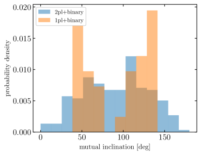
Figure 9: Mutual inclination between the orbit of the binary and of the planet, for systems where the latter has $e\geq 0.84$ at the end of the simulation.

One potential observational means of distinguishing between the pure Kozai, versus the scattering plus Kozai, dynamical histories, lies in the mutual inclination of the planet and the binary companion at the present time. The probability distributions of mutual inclination at the end of the simulation are shown in Figure 9, for the 1pl+binary-weighted and the 2pl+binary-weighted simulation sets where the surviving planet ends with an eccentricity $\geq 0.84$. We see that in the single-planet case, where the orbital evolution is heavily constrained by starting at low-eccentricity, the range of mutual inclinations in the high-eccentricity systems is rather limited, with both polar and low-inclination configurations being prohibited. In contrast, in the two-planet systems, the final mutual inclination between the surviving eccentric planet and the binary roughly follows an isotropic distribution. Thus, if the inclination of the planet’s orbit can be measured or constrained (by astrometric measurement of the star’s reflex motion with Gaia, or else by direct imaging), a polar or low-inclination configuration at the present day would be inconsistent with the single-planet origin, and support an earlier scattering history.

4.3 Effects of short-range forces

We have modelled the orbital dynamics with pure Newtonian point-mass dynamics. However, in highly-eccentric systems short-range forces can become significant. Two such forces are those that arise from general relativity, and from tidal deformation of the bodies.

Orbits in the relativistic two-body problem are subjected to a slow precession due to the leading-order effects of general relativity. In the three-body problem, this can suppress the excitation of eccentricity through Lidov–Kozai cycles (e.g., Holman et al., 1997). The precession rate of an eccentric orbit under GR precession is given by (e.g., Naoz, 2016):

$$\frac{\mathrm{d}\omega}{\mathrm{d}t}=\frac{3k^{3}M_{\star}^{3/2}}{a^{5/2}c^{2}\left(1-e^{2}\right)},$$ (2)

where $k$ is the Gaussian gravitational constant and $c$ the speed of light. This precession rate yields a timescale for one cycle of precession of 42 Gyr, for the planet at 18 au, if its eccentricity is zero, and 12 Gyr if its eccentricity is $0.84$. As the timescale for Lidov–Kozai cycles must be $\lesssim 8$ Gyr, the system age, to significantly change the planet’s eccentricity, the effects of GR should not significantly affect the Lidov–Kozai dynamics of those systems that are affected on astrophysically relevant timescales.

Tidal distortion of one or both bodies can also cause apsidal precession. The rate is given by

$$\frac{\mathrm{d}\omega}{\mathrm{d}t} = \frac{15\sqrt{\mathscr{G}\left(M_{\star}+M_{\mathrm{b}}\right)}}{8a^{13/2}}\frac{8+12e^{2}+e^{4}}{\left(1-e^{2}\right)^{5}}$$ (4)

$$\left(\frac{M_{\mathrm{b}}}{M_{\star}}k_{\star}R_{\star}^{5}+\frac{M_{\star}}{M_{\mathrm{b}}}k_{\mathrm{b}}R_{\mathrm{b}}^{5}\right),$$

where $k_{\star}$ and $k_{\mathrm{b}}$ are the Love numbers of the star and the planet, and $\mathscr{G}$ is the gravitational constant (Fabrycky & Tremaine, 2007). At $e=0.84$, we find for this system a precession time of $1.5\times 10^{17}$ yr for one cycle, when assuming a planetary radius of 1 Jupiter radius and unrealistically high values of $k_{\star}=k_{\mathrm{b}}=1$. Hence, for our purposes, tidal effects are negligible, although they would affect the small number of planets that end up colliding with the star, and the rate of formation of Hot Jupiters through the different dynamical channels.

4.4 Caveats on orbital evolution of the binary

In this paper, we have treated the orbit of the binary as unchanging. This has enabled us to isolate the effect Lidov–Kozai cycles from a binary perturber on a fixed orbit have on the planet after scattering, without worrying about changes to the binary orbit through the Galactic tide or stellar flybys, or indeed about the breakup of the binary by passing stars. Here, we note that the binary has clearly survived several Gyr without disruption. Binaries at $a=10^{4}$ au are disrupted at a rate of $\sim 50\%$ per $10\mathrm{\,Gyr}$ (Kaib et al., 2013; Correa-Otto & Gil-Hutton, 2017). While the binary has avoided this, it may have had its orbit changed, a process more likely if the stars were formed at smaller Galactocentric radii than their present orbit where field star densities are higher, before migrating outwards (Wielen et al., 1996; Sellwood & Binney, 2002; Nieva & Przybilla, 2012; Kubryk et al., 2015; Frankel et al., 2018). Formation closer to the Galactic centre may be likely based on the star’s slightly super-Solar metallicity, but the extent (and even necessity) of migration for the Sun at least is disputed (e.g., Minchev et al., 2018; Haywood et al., 2019; Frankel et al., 2020), depending on assumptions about the enrichment history of the ISM. Kaib et al. (2013) show that a doubling or quadrupling of field star densities, as would be expected if formation were several kpc closer to the Galactic centre, leads to a moderate increase in the fraction of planetary systems destabilised by wide binaries; however, Correa-Otto & Gil-Hutton (2017) show that, despite perturbations to their orbits, even highly eccentric binaries at $\sim 10^{4}$ au are unlikely to directly destabilise planets within 30 au. Hence, the binaries most effective at exciting high eccentricity through the Kozai mechanism (having lower $a$ and higher $e$), and which have avoided being broken up by flybys in the field, will also have avoided penetrating too deeply into the inner system to directly destabilise any planets. The most likely effect of considering changes to the binary orbit, then, would be some modulation of the Lidov–Kozai timescale as the binary orbital elements are perturbed.

4.5 Other systems

The mechanism of eccentricity excitation by scattering plus Lidov–Kozai interaction that we have described in this paper will not be limited to the HR 5183 system. While close (within a few tens of au) binary companions are expected to hinder the planet formation process (e.g., Jang-Condell, 2015; Marzari & Thebault, 2019), this is not expected for the wider binary systems. Indeed, observationally, the binary companions of exoplanet systems seem to have a wider semimajor axis distribution than the companions of field stars chosen without reference to their exoplanet systems. This is seen in studies of transiting planetary systems (Kraus et al., 2016; Ziegler et al., 2020; Howell et al., 2021), as well as of giant planets within a few au of their host star (Fontanive et al., 2019; Hirsch et al., 2020). Meanwhile, the masses and semimajor axes of planets in binaries wider than 1 000 au are the same as those of planets orbiting single stars (Fontanive & Bardalez Gagliuffi, 2021). Of particular relevance is the study of the binary companions to white dwarfs with photospheric metal lines by Zuckerman (2014): these “polluted” white dwarfs are thought to be displaying the traces of asteroids or planetary remnants scattered into the white dwarf’s atmosphere (e.g., Alcock et al., 1986; Debes & Sigurdsson, 2002; Jura & Young, 2014; Farihi, 2016). The source region for these bodies must be several to several tens of au in order to survive the host star’s asymptotic giant branch evolution (Mustill & Villaver, 2012; Mustill et al., 2018) – exactly the semimajor axis range of HR 5183b. For these systems, Zuckerman (2014) found that binary companions beyond 1000 au seem not to suppress the existance of planetary systems; a similar result was found by Wilson et al. (2019). This raises hopes that more systems similar to HR 5183, with a planet at  10 au and a wide binary beyond 1000 au, may be found.

Indeed, the NASA Exoplanet Archive lists 16 planets with an eccentricity $e\geq 0.8$. Of these, 8 are listed as being in multiple star systems (HD 28254 b, Naef et al. 2010; HR 5183 b, Blunt et al. 2019; HD 108341 b, Moutou et al. 2015; HD 156846 b, Stassun et al. 2017; HD 4113 b, Tamuz et al. 2008; HD 7449 b, Wittenmyer et al. 2019; HD 80606 b, Stassun et al. 2017; and HD 20782 b, Udry et al. 2019). While this is a small and possibly biased sample, this fraction of high-eccentricity planets with binary companions (50%) is much higher than the fraction of all planetary systems in multiple stellar systems (321 out of 3213, or 10%). This suggests a role of stellar binarity in generating these very large eccentricities, which we have shown is easier if the planetary system began with multiple planets and underwent scattering.

Finally, we note that Kane & Blunt (2019) showed that it is possible for a terrestrial planet to remain on a stable orbit in the Habitable Zone of the HR5183 system, under the perturbations from the known planet on its current orbit. However, Matsumura et al. (2013); Carrera et al. (2016); Kokaia et al. (2020) have shown that treating a known planet’s orbit as fixed gives an optimistic estimate of the survivability of Habitable Zone planets, in the case of planet–planet scattering. Future studies should re-evaluate the prospects for the existence of such planets in HR5183 and similar systems under the different possible dynamical evolution scenarios.

5 Conclusions

We have examined and compared the efficiencies of three mechanisms of exciting an exoplanet’s orbit to high eccentricity: scattering in an unstable two-planet system, Lidov–Kozai forcing from a wide stellar binary companion, and a combination of planet–planet scattering plus Lidov–Kozai cycles from a wide binary. We have reproduced the current orbital configuration of the HR 5183 system with these three mechanisms, with the following quantitive success rates (planetary eccentricity at the end of the simulation $\geq 0.84$, its current value):

• Two-planet scattering: $2.8-7.2\%$ of unstable systems end up with a planet with $e\geq 0.84$. The success rate depends on the mass ratio between the outer and inner planets, being lowest for equal-mass planets and peaking for a mass ratio $\sim 1.5$.

• Single-planet Lidov–Kozai: $0.6\%$ of systems end up with a planet with $e\geq 0.84$.

• Two-planet scattering plus Lidov–Kozai: $14.5\%$ of unstable systems with equal-mass planets end up with a planet with $e\geq 0.84$.

Given the existence of the comoving and probably bound companion star to HR5183, we consider that planet–planet scattering followed by Lidov–Kozai cycles driven by the binary is the best explanation of the planet’s high eccentricity. This can potentially be tested if the inclination of the planet’s orbit can be measured, since eccentricity excitation by Lidov–Kozai cycles from a circular orbit in a single-planet system leads to neither coplanar nor polar orbits, whereas Lidov–Kozai cycles acting after planet–planet scattering has occurred permit any mutual inclination between the surviving planet and the binary companion. Given that wide binaries such as the system we have studied are observed to happily coexist with planetary systems, this combination of planet–planet scattering and Lidov–Kozai cycles may affect the eccentricities of many wide-orbit giant planets. Indeed, the existing small sample of highly-eccentric planets suggests that these are more likely to be found in binary stellar systems.

Data availability statement

The data underlying this paper will be made available on reasonable request to the corresponding author.

Note added in proof

Following the acceptance of this paper, Venner et al. (2021) published an improved orbital fit for both the planet and the binary companion to HR5183, with tentative but not statistically significant evidence for orbital misalignment. Future astrometry should refine the orbital misalignment angle further.

References

- Alcock et al. (1986) Alcock C., Fristrom C. C., Siegelman R., 1986, ApJ, 302, 462
- Allen et al. (2000) Allen C., Poveda A., Herrera M. A., 2000, A&A, 356, 529
- Astropy Collaboration et al. (2013) Astropy Collaboration et al., 2013, A&A, 558, A33
- Astropy Collaboration et al. (2018) Astropy Collaboration et al., 2018, aj, 156, 123
- Blunt et al. (2019) Blunt S., et al., 2019, AJ, 158, 181
- Bohn et al. (2020) Bohn A. J., et al., 2020, ApJ, 898, L16
- Boué & Fabrycky (2014) Boué G., Fabrycky D. C., 2014, ApJ, 789, 111
- Carrera et al. (2016) Carrera D., Davies M. B., Johansen A., 2016, MNRAS, 463, 3226
- Carrera et al. (2019) Carrera D., Raymond S. N., Davies M. B., 2019, A&A, 629, L7
- Chambers (1999) Chambers J. E., 1999, MNRAS, 304, 793
- Chambers et al. (1996) Chambers J. E., Wetherill G. W., Boss A. P., 1996, Icarus, 119, 261
- Chatterjee et al. (2008) Chatterjee S., Ford E. B., Matsumura S., Rasio F. A., 2008, ApJ, 686, 580
- Correa-Otto & Gil-Hutton (2017) Correa-Otto J. A., Gil-Hutton R. A., 2017, A&A, 608, A116
- Debes & Sigurdsson (2002) Debes J. H., Sigurdsson S., 2002, ApJ, 572, 556
- Denham et al. (2019) Denham P., Naoz S., Hoang B.-M., Stephan A. P., Farr W. M., 2019, MNRAS, 482, 4146
- Everhart (1985) Everhart E., 1985, An efficient integrator that uses Gauss-Radau spacings. p. 185, doi:10.1007/978-94-009-5400-7_17
- Fabrycky & Tremaine (2007) Fabrycky D., Tremaine S., 2007, ApJ, 669, 1298
- Farihi (2016) Farihi J., 2016, New Astron. Rev., 71, 9
- Fontanive & Bardalez Gagliuffi (2021) Fontanive C., Bardalez Gagliuffi D., 2021, Frontiers in Astronomy and Space Sciences, 8, 16
- Fontanive et al. (2019) Fontanive C., Rice K., Bonavita M., Lopez E., Mužić K., Biller B., 2019, MNRAS, 485, 4967
- Forgan et al. (2018) Forgan D. H., Hall C., Meru F., Rice W. K. M., 2018, MNRAS, 474, 5036
- Frankel et al. (2018) Frankel N., Rix H.-W., Ting Y.-S., Ness M., Hogg D. W., 2018, ApJ, 865, 96
- Frankel et al. (2020) Frankel N., Sanders J., Ting Y.-S., Rix H.-W., 2020, ApJ, 896, 15
- Gaia Collaboration et al. (2016) Gaia Collaboration et al., 2016, A&A, 595, A1
- Gaia Collaboration et al. (2018) Gaia Collaboration et al., 2018, A&A, 616, A1
- Gaia Collaboration et al. (2021) Gaia Collaboration et al., 2021, A&A, 649, A1
- Gladman (1993) Gladman B., 1993, Icarus, 106, 247
- Hall et al. (2017) Hall C., Forgan D., Rice K., 2017, MNRAS, 470, 2517
- Harris et al. (2012) Harris R. J., Andrews S. M., Wilner D. J., Kraus A. L., 2012, ApJ, 751, 115
- Harris et al. (2020) Harris C. R., et al., 2020, Nature, 585, 357–362
- Haywood et al. (2019) Haywood M., Snaith O., Lehnert M. D., Di Matteo P., Khoperskov S., 2019, A&A, 625, A105
- Hirsch et al. (2020) Hirsch L. A., et al., 2020, arXiv e-prints, p. arXiv:2012.09190
- Holman et al. (1997) Holman M., Touma J., Tremaine S., 1997, Nature, 386, 254
- Howell et al. (2021) Howell S. B., Matson R. A., Ciardi D. R., Everett M. E., Livingston J. H., Scott N. J., Horch E. P., Winn J. N., 2021, arXiv e-prints, p. arXiv:2101.08671
- Hunter (2007) Hunter J. D., 2007, Computing in Science and Engineering, 9, 90
- Innanen et al. (1997) Innanen K. A., Zheng J. Q., Mikkola S., Valtonen M. J., 1997, AJ, 113, 1915
- Jang-Condell (2015) Jang-Condell H., 2015, ApJ, 799, 147
- Jura & Young (2014) Jura M., Young E. D., 2014, Annual Review of Earth and Planetary Sciences, 42, 45
- Jurić & Tremaine (2008) Jurić M., Tremaine S., 2008, ApJ, 686, 603
- Kaib et al. (2011) Kaib N. A., Raymond S. N., Duncan M. J., 2011, ApJ, 742, L24
- Kaib et al. (2013) Kaib N. A., Raymond S. N., Duncan M., 2013, Nature, 493, 381
- Kane & Blunt (2019) Kane S. R., Blunt S., 2019, AJ, 158, 209
- Kokaia et al. (2020) Kokaia G., Davies M. B., Mustill A. J., 2020, MNRAS, 492, 352
- Kozai (1962) Kozai Y., 1962, AJ, 67, 591
- Kraus et al. (2016) Kraus A. L., Ireland M. J., Huber D., Mann A. W., Dupuy T. J., 2016, AJ, 152, 8
- Kubryk et al. (2015) Kubryk M., Prantzos N., Athanassoula E., 2015, A&A, 580, A126
- Lidov (1962) Lidov M. L., 1962, Planet. Space Sci., 9, 719
- Malmberg et al. (2007) Malmberg D., Davies M. B., Chambers J. E., 2007, MNRAS, 377, L1
- Marois et al. (2008) Marois C., Macintosh B., Barman T., Zuckerman B., Song I., Patience J., Lafrenière D., Doyon R., 2008, Science, 322, 1348
- Marzari & Thebault (2019) Marzari F., Thebault P., 2019, Galaxies, 7, 84
- Matsumura et al. (2013) Matsumura S., Ida S., Nagasawa M., 2013, ApJ, 767, 129
- Minchev et al. (2018) Minchev I., et al., 2018, MNRAS, 481, 1645
- Moutou et al. (2015) Moutou C., et al., 2015, A&A, 576, A48
- Mustill & Villaver (2012) Mustill A. J., Villaver E., 2012, ApJ, 761, 121
- Mustill et al. (2017) Mustill A. J., Davies M. B., Johansen A., 2017, MNRAS, 468, 3000
- Mustill et al. (2018) Mustill A. J., Villaver E., Veras D., Gänsicke B. T., Bonsor A., 2018, MNRAS, 476, 3939
- Naef et al. (2010) Naef D., et al., 2010, A&A, 523, A15
- Naoz (2016) Naoz S., 2016, ARA&A, 54, 441
- Nieva & Przybilla (2012) Nieva M. F., Przybilla N., 2012, A&A, 539, A143
- Petit et al. (2020) Petit A. C., Pichierri G., Davies M. B., Johansen A., 2020, A&A, 641, A176
- Pu & Lai (2018) Pu B., Lai D., 2018, MNRAS, 478, 197
- Quillen (2011) Quillen A. C., 2011, MNRAS, 418, 1043
- Raghavan et al. (2010) Raghavan D., et al., 2010, ApJS, 190, 1
- Rasio & Ford (1996) Rasio F. A., Ford E. B., 1996, Science, 274, 954
- Raymond et al. (2011) Raymond S. N., et al., 2011, A&A, 530, A62
- Sellwood & Binney (2002) Sellwood J. A., Binney J. J., 2002, MNRAS, 336, 785
- Stassun et al. (2017) Stassun K. G., Collins K. A., Gaudi B. S., 2017, AJ, 153, 136
- Tamuz et al. (2008) Tamuz O., et al., 2008, A&A, 480, L33
- Tokovinin & Lépine (2012) Tokovinin A., Lépine S., 2012, AJ, 144, 102
- Udry et al. (2019) Udry S., et al., 2019, A&A, 622, A37
- Venner et al. (2021) Venner A., Pearce L. A., Vanderburg A., 2021, arXiv e-prints, p. arXiv:2111.03676
- Veras & Mustill (2013) Veras D., Mustill A. J., 2013, MNRAS, 434, L11
- Virtanen et al. (2020) Virtanen P., et al., 2020, Nature Methods, 17, 261
- Weidenschilling & Marzari (1996) Weidenschilling S. J., Marzari F., 1996, Nature, 384, 619
- Wielen et al. (1996) Wielen R., Fuchs B., Dettbarn C., 1996, A&A, 314, 438
- Wilson et al. (2019) Wilson T. G., Farihi J., Gänsicke B. T., Swan A., 2019, MNRAS, 487, 133
- Wittenmyer et al. (2019) Wittenmyer R. A., Clark J. T., Zhao J., Horner J., Wang S., Johns D., 2019, MNRAS, 484, 5859
- Ziegler et al. (2020) Ziegler C., Tokovinin A., Briceño C., Mang J., Law N., Mann A. W., 2020, AJ, 159, 19
- Zuckerman (2014) Zuckerman B., 2014, ApJ, 791, L27