General Law of iterated logarithm for Markov processes: Limsup law

Abstract.

In this paper, we discuss general criteria of limsup law of iterated logarithm (LIL) for continuous-time Markov processes. We consider minimal assumptions for LILs to hold at zero (at infinity, respectively) in general metric measure spaces. We establish LILs under local assumptions near zero (near infinity, respectively) on uniform bounds of the expectations of first exit times from balls in terms of a function $\phi$ and uniform bounds on the tails of the jumping kernel in terms of a function $\psi$. The main result is that a simple ratio test in terms of the functions $\phi$ and $\psi$ completely determines whether there exists a positive non-decreasing function $\Psi$ such that $\limsup|X_{t}|/\Psi(t)$ is positive and finite a.s., or not. Our results cover a large class of subordinate diffusions, jump processes with mixed polynomial local growths, jump processes with singular jumping kernels and random conductance models with long range jumps.

Keywords: limsup law; jump processes; law of the iterated logarithm; sample path;

MSC 2020: 60J25; 60J35; 60J76; 60F15; 60F20.

1. Introduction and general result

Law of the iterated logarithm (LIL) for a stochastic process describes the magnitude of the fluctuations of its sample path behaviors. In addition to the law of large numbers and the central limit theorem, the LIL is considered the fundamental limit theorem in Probability theory. See [27] and the references therein.

Let $Y:=(Y_{t})_{t\geq 0}$ be a non-trivial strictly $\beta$-stable process on ${\mathbb{R}}^{d}$ with $0<\beta\leq 2$ in the sense of [58, Definition 13.1]. Then $Y$ satisfies the following well known limsup LIL: If $\beta=2$, then there exist constants $c_{1},c_{2}\in(0,\infty)$ such that

$$\limsup_{t\to 0\;\;(\text{resp. }t\to\infty)}\frac{\sup_{0<s\leq t}|Y_{s}|}{(t\log|\log t|)^{1/\beta}}=c_{1},\quad\limsup_{t\to 0\;\;(\text{resp. }t\to\infty)}\frac{|Y_{t}|}{(t\log|\log t|)^{1/\beta}}=c_{2}\;\;\mbox{ a.s.}$$ (1.1)

Otherwise, i.e., $\beta<2$, then for every positive non-decreasing function $\Psi$,

$$\begin{split}&\int_{0}\Psi(t)^{-\beta}dt<\infty\;\;\text{ or }\;\;=\infty\quad\Big{(}{\rm resp.}\int^{\infty}\Psi(t)^{-\beta}dt<\infty\;\;\text{ or }\;\;=\infty\Big{)}\\ &\Leftrightarrow\;\;\limsup_{t\to 0\;\;(\text{resp. }t\to\infty)}\frac{\sup_{0<s\leq t}|Y_{s}|}{\Psi(t)}=\limsup_{t\to 0\;\;(\text{resp. }t\to\infty)}\frac{|Y_{t}|}{\Psi(t)}=0\;\;\text{ or }\;\;\infty,\;\;\mbox{ a.s.}\end{split}$$ (1.2)

See [58, Chapters 47, 48] and the references therein.

The limsup LIL of the second type (for $|Y_{t}|$) in (1.1) was obtained by Khintchine [43], Kolmogorov [49], Hartman and Wintner [39] and Lévy [51], for various random walks and Brownian motions in any dimension. The limsup LIL of the first type (for $\sup_{0<s\leq t}|Y_{s}|$) in (1.1) was obtained by Strassen [62] for some random walks and Brownian motion in ${\mathbb{R}}^{1}$. Later, Barlow and Perkins [9] and Barlow [4] showed that the limsup LIL of the second type holds with some $\beta\geq 2$ for Brownian motions on some fractals including Sierpinski gasket or carpet, and Bass and Kumagai [10] showed that the first type holds for Brownian motions on some fractals and Riemannian manifolds. (Although these results only consider either $t$ tends to zero or infinity, one can prove the results for the other direction by modifying their proofs.) For jump processes (Markov processes whose trajectories have discontinuities), the limsup LIL of the second type at infinity was done for Lévy processes in ${\mathbb{R}}$ with finite second moment by Gnedenko [32], symmetric stable processes in ${\mathbb{R}}$ without large jumps by Griffin [33], and non-Lévy processes in ${\mathbb{R}}^{d}$ with finite second moment by Shiozawa and Wang [61], and Bae, Kang, Kim and Lee [2]. Very recently, the work on limsup LIL at infinity in [2] is extended by same authors to metric measure space in [3].

The limsup LIL of type (1.2) was first obtained by Khintchine [44] in ${\mathbb{R}}$. Those results were extended to subordinators and some Lévy processes in ${\mathbb{R}}$ by Fristedt [29, 30]. Recently, the limsup LILs of type (1.2) at zero were discussed for more general Lévy processes in ${\mathbb{R}}$ by Savov [59] and some Lévy-type processes in ${\mathbb{R}}$ by Knopova and Schilling [48]. We refer to [45] for a multi-dimensional version.

In the study of the limsup laws, the following natural and important question has been raised and partially answered. Cf. questions in [26, 40, 56, 55] for random walks. We denote by ${\cal M}_{+}$ the set of all positive non-decreasing functions defined on $(0,c_{1}]\cup[c_{2},\infty)$ for some $c_{2}\geq c_{1}>0$.

$\mathbf{(Q)}$ How do we determine that a limsup law (either at zero or at infinity) of a given process $Y$ is of type (1.1), or else of type (1.2)? More precisely, what is a necessary and sufficient condition for the existence of $\Psi\in{\cal M}_{+}$ such that $\limsup$ of $|Y_{t}|/\Psi(t)$ converges to a positive, finite and deterministic value as $t$ tends to zero or infinity?

Feller [28] studied the above question for symmetric random walks which belong to the domain of attraction of the normal distribution, and established an integral test as an answer. He also found the exact form of $\Psi$ when it exists. We also refer to Kesten’s work [42]. For continuous time processes, Fristedt [30] partially answered the above question for one-dimensional symmetric Lévy processes. Then Wee and Kim [64] established a ratio test for entire one-dimensional Lévy processes which determine whether $\limsup|Y_{t}|/\Psi(t)\in(0,\infty)$.

The purpose of this paper is to understand asymptotic behaviors of a given Markov process by establishing limsup law of iterated logarithms for both near zero and near infinity under some minimal assumptions. The main contribution of this paper is that we answer the above question ${\bf(Q)}$ completely for a large class of Markov processes including random conductance models with stable-like jumps (see Theorems 1.9–1.10 and Section 3 below).

Formally, our answer is

$\mathbf{(A)}$ There is a dichotomous classification on continuous time Markov processes (satisfying a near diagonal lower bound estimate for the Dirichlet heat kernel): Based on whether the tails of the jumping kernel and the mean exit times (the expectation of first exit times) from balls are comparable or not, we can categorize Markov processes into two non-overlapping classes ${\cal A}^{\infty}_{1}$ and ${\cal A}^{\infty}_{2}$:

$${\cal A}^{\infty}_{1}=\Big{\{}\text{For all }\Psi\in{\cal M}_{+},\;\,\limsup_{t\to\infty}\frac{d(x,X_{t})}{\Psi(t)}\text{ is either $0$ for all $x$, or $\infty$ for all $x$.}\Big{\}},$$

$${\cal A}^{\infty}_{2}=\Big{\{}\text{There is $\Psi\in{\cal M}_{+}$ such that }\limsup_{t\to\infty}\frac{d(x,X_{t})}{\Psi(t)}\text{ is deterministic and in $(0,\infty)$ for all $x$.}\Big{\}}$$

If a given Markov process $X$ is in the class ${\cal A}^{\infty}_{1}$, then there is an integral test that determines whether the above $\limsup$ is zero or infinite. If a given Markov process $X$ is in the class ${\cal A}^{\infty}_{2}$, then there is a natural explicit function $\Psi$ and another integral test to determine when one can take such specific $\Psi$. An analogous result holds for $\limsup$ LIL at zero.

The reader will see that processes near the borderline of the above classes are so-called Brownian-like jump processes, i.e., jump processes with high intensity of small jumps and ones with low intensity of large jumps.

Assumptions in this paper are motivated by the second named author’s previous paper [45]. In [45], the authors established liminf and limsup LILs (of type (1.2)) for Feller processes on a general metric measure space enjoying mixed stable-like heat kernel estimates (see Assumption 2.1 therein). Recently, relationships among those heat kernel estimates, and certain conditions on the jumping kernel and the mean exit time from open balls are extensively studied. See, e.g. [3, 2, 17, 18, 19, 8, 34]. We adopt this framework and consider localized and relaxed conditions not only on the heat kernel but also on the jumping kernel and the mean exit time. We emphasize that, unlike the references mentioned above, we do not assume a weak lower scaling property of the scale function $\phi$ in several statements. (See Definition 1.8 for the notion of weak lower scaling property.) However, we still need the weak lower scaling property in some other statements, especially ones concerning long time behaviors.

Our assumptions are weak enough so that our results cover a lot of Markov processes including random conductance models with long range jumps, jump processes with diffusion part, jump processes with low intensity of small jumps, some non-symmetric processes and processes with singular jumping kernels. See the examples in Sections 2 and 3, and also see [23] for further examples. In particular, the class of Markov processes considered in this paper extends the corresponding results of [45] significantly. Moreover, metric measure spaces in this paper can be random, disconnected and highly space-inhomogeneous (see Definition 1.1).

Let us now describe the main result of this paper precisely and, at the same time, fix the setup and the notation of the paper.

Throughout this paper, we assume that $(M,d)$ is a locally compact separable metric space with a base point $o\in M$, and $\mu$ is a positive Radon measure on $M$ with full support. Denote by $B(x,r):=\{y\in M:d(x,y)<r\}$ and $V(x,r):=\mu(B(x,r))$ an open ball in $M$ and its volume, respectively. We add a cemetery point $\partial$ to $M$ and define $M_{\partial}:=M\cup\{\partial\}$. Any function $f$ on $M$ is extended to $M_{\partial}$ by setting $f(\partial)=0$.

For an open set $U\subset M$ and $x\in M$, we denote by $\updelta_{U}(x)$ the distance between $x$ and $M\setminus U$. We define a map ${\mathsf{d}}:M\to[1,\infty)$ by

$${\mathsf{d}}(x):=d(x,o)+1.$$

When $M={\mathbb{R}}^{d}$ and $o$ is the origin, ${\mathsf{d}}(x)$ equals to $|x|+1$. Note that the map ${\upsilon}\mapsto{\mathsf{d}}(x)^{\upsilon}$ is non-decreasing on ${\mathbb{R}}$ since ${\mathsf{d}}(x)\geq 1$.

We now introduce following versions of volume doubling property. We denote $a\land b$ for $\min\{a,b\}$ and $a\vee b$ for $\max\{a,b\}$.

Definition 1.1.

(i) For an open set $U\subset M$ and $R_{0}\in(0,\infty]$, we say that the interior volume doubling and reverse doubling property near zero ${\mathrm{VRD}}_{R_{0}}(U)$ holds (with $C_{V}$) if there exist constants $C_{V}\in(0,1)$, $d_{2}\geq d_{1}>0$ and $c>1$ such that for all $x\in U$ and $0<s\leq r<R_{0}\land(C_{V}\updelta_{U}(x))$,

$$c^{-1}\Big{(}\frac{r}{s}\Big{)}^{d_{1}}\leq\frac{V(x,r)}{V(x,s)}\leq c\Big{(}\frac{r}{s}\Big{)}^{d_{2}}.$$ (1.3)

(ii) For $R_{\infty}\geq 1$, we say that the weak volume doubling and reverse doubling property near infinity ${\mathrm{VRD}}^{R_{\infty}}$ holds if there exist constants ${\upsilon}\in(0,1)$, $d_{2}\geq d_{1}>0$ and $c>1$ such that (1.3) holds for all $x\in M$ and $r\geq s>R_{\infty}{\mathsf{d}}(x)^{\upsilon}$.

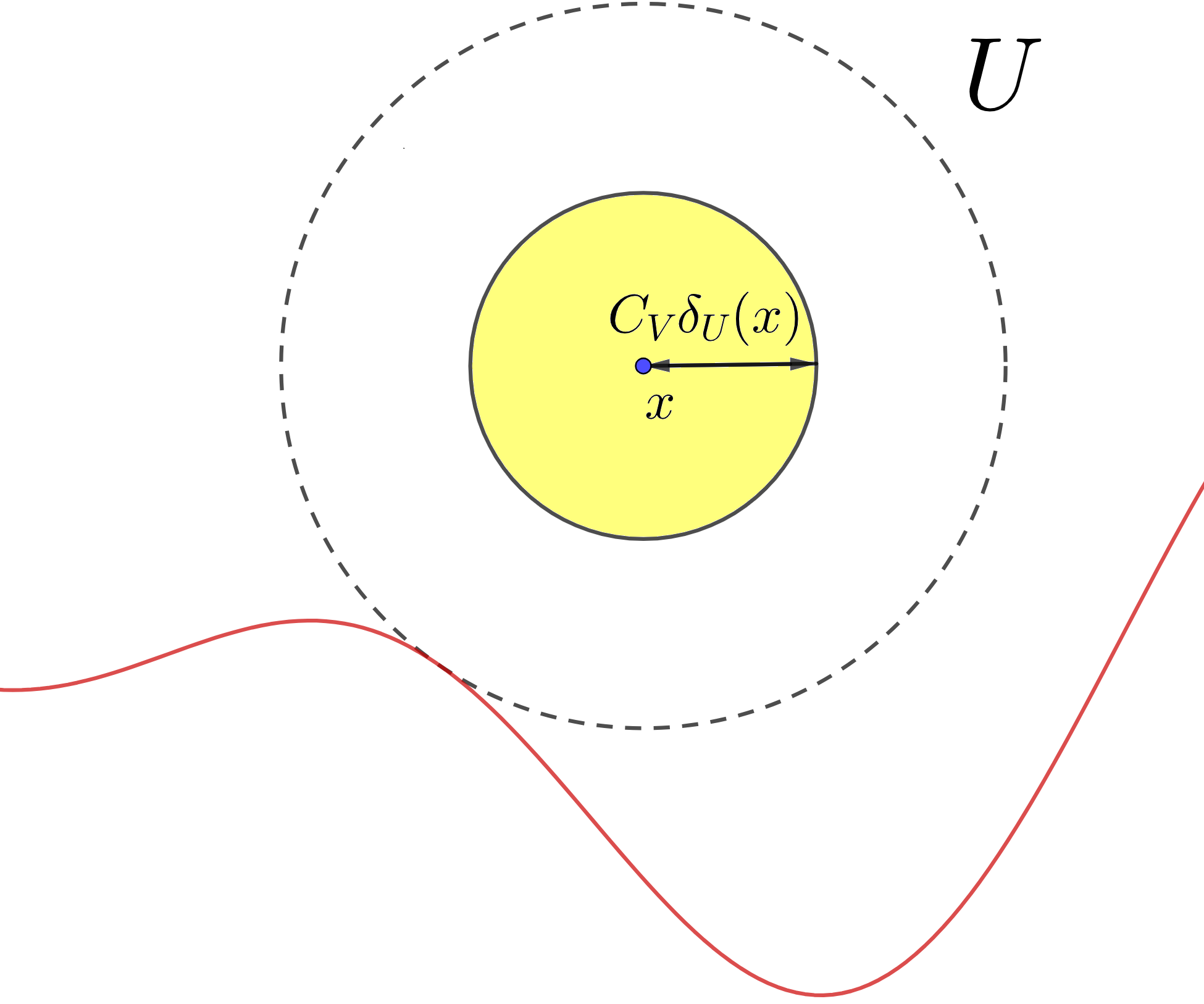
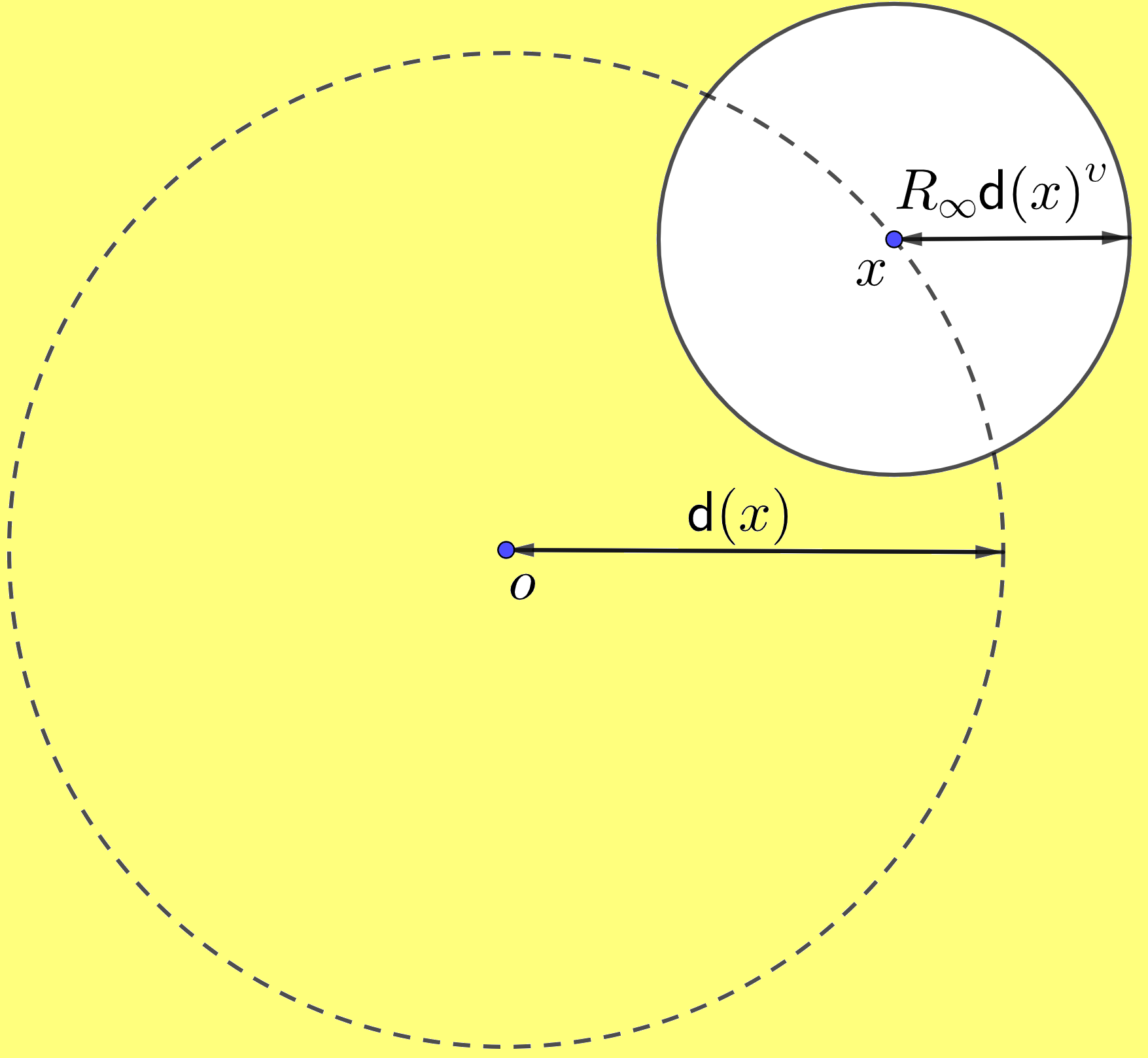
Figure 1. Range of $r$ in local conditions

Note that, under ${\mathrm{VRD}}_{R_{0}}(U)$ (resp. ${\mathrm{VRD}}^{R_{\infty}}$), it holds that with a constant $\ell:=(2/c_{\mu})^{1/d_{1}}$,

$$\frac{V(x,r)}{V(x,r/\ell)}\geq 2\;\;\mbox{ for all}\;x\in U\mbox{ and }0<r<R_{0}\land(C_{V}\updelta_{U}(x))\;\;\big{(}\text{resp. }x\in M\mbox{ and }r>\ell R_{\infty}{\mathsf{d}}(x)^{\upsilon}\big{)}.$$ (1.4)

Next, we define local versions of the so-called chain condition.

Definition 1.2.

(i) For an open set $U\subset M$ and $R_{0}\in(0,\infty]$, we say that the chain condition near zero $\mathrm{Ch}_{R_{0}}(U)$ holds if there exists a constant $A\geq 1$ such that for all $x,y\in U$ with $d(x,y)<R_{0}$ and $n\in{\mathbb{N}}$, there is a sequence $(z_{i})_{0\leq i\leq n}\subset M$ such that

$$z_{0}=x,\;\;z_{n}=y\;\;\text{and}\;\;d(z_{i-1},z_{i})\leq\frac{A}{n}d(x,y)\quad\text{for all}\;\;1\leq i\leq n.$$ (1.5)

(ii) For $R_{\infty}\geq 1$, we say that the weak chain condition near infinity $\mathrm{Ch}^{R_{\infty}}$ holds if there exist constants ${\upsilon}\in(0,1)$ and $A\geq 1$ such that for all $x,y\in M$ and $n\in{\mathbb{N}}$ with $d(x,y)/n>R_{\infty}({\mathsf{d}}(x)\vee{\mathsf{d}}(y))^{\upsilon}$, there is a sequence $(z_{i})_{0\leq i\leq n}\subset M$ satisfying (1.5).

Remark 1.3.

If $(M,d)$ is geodesic, then $\mathrm{Ch}_{\infty}(M)$ clearly holds.

Let $X=(\Omega,{\cal F}_{t},X_{t},\theta_{t},t\geq 0;{\mathbb{P}}^{x},x\in M_{\partial})$ be a Borel standard Markov process on $M_{\partial}$ with the lifetime $\zeta:=\inf\{t>0:X_{t}=\partial\}$. Here $(\theta_{t},t\geq 0)$ is the shift operator with respect to $X$, which is defined as $X_{s}(\theta_{t}\,\omega)=X_{s+t}(\omega)$ for $t,s>0$ and $\omega\in\Omega$. A family of $[0,\infty]$-valued random variables $\mathfrak{A}=(\mathfrak{A}_{t},t\geq 0)$ is called a positive continuous additive functional (PCAF) (in the strict sense) of $X$, if there exists $\Lambda\in{\cal F}_{\infty}$ with ${\mathbb{P}}^{x}(\Lambda)=1$ for all $x\in M$ such that the following conditions are satisfied: (i) For each $t\geq 0$, $\mathfrak{A}_{t}|_{\Lambda}$ is ${\cal F}_{t}|_{\Lambda}$-measurable and (ii) For any $\omega\in\Lambda$, $\mathfrak{A}_{0}(\omega)=0$, $|\mathfrak{A}_{t}(\omega)|<\infty$ for $t<\zeta(\omega)$, $\mathfrak{A}_{t}(\omega)=\mathfrak{A}_{\zeta(\omega)}(\omega)$ for $t\geq\zeta(\omega)$, $t\mapsto\mathfrak{A}_{t}(\omega)$ is a continuous function on $[0,\infty]$ and $\mathfrak{A}_{t+s}(\omega)=\mathfrak{A}_{t}(\omega)+\mathfrak{A}_{s}(\theta_{t}\,\omega)$ for all $s,t\geq 0$. See [31, Chapter 5].

According to [11], since $X$ is a Borel standard process on $M$, it has a Lévy system $(N,H)$. Here $N(x,dy)$ is a kernel on $(M_{\partial},{\cal B}(M_{\partial}))$ and $H$ is a PCAF of $X$ with bounded $1$-potential. We assume that $X$ has a Lévy system $(N,H)$ such that the Revuz measure of $H$ is given by $\nu_{H}(x)\mu(dx)$ for a measurable function $\nu_{H}(x)$. Let $J(x,dy)=N(x,dy)\nu_{H}(x)$. Then, by the Lévy system formula, for any non-negative Borel function $F$ on $M\times M_{\partial}$ vanishing on the diagonal, it holds that

$${\mathbb{E}}^{z}\bigg{[}\sum_{s\leq t}F(X_{s-},X_{s})\bigg{]}={\mathbb{E}}^{z}\left[\int_{0}^{t}\int_{M_{\partial}}F(X_{s},y)J(X_{s},dy)ds\right],\quad z\in M,\;t>0.$$ (1.6)

The measure $J(x,dy)$ on $M_{\partial}$ is called the Lévy measure of $X$. See [63]. Here, we note that the killing term $J(x,\partial)$ is included in the Lévy measure. Also, we emphasize that $J(x,dy)$ can be identically zero and $J(x,dy)$ may not be absolutely continuous with respect to $\mu$.

For an open set $D\subset M$, denote by $\tau_{D}:=\inf\{t>0:X_{t}\in M_{\partial}\setminus D\}$ the first exit time of $X$ from $D$. The subprocess $X^{D}$, defined by $X_{t}^{D}:=X_{t}\,{\bf 1}_{\{\tau_{D}>t\}}+\partial\,{\bf 1}_{\{\tau_{D}\leq t\}}$, is called the killed process of $X$ upon leaving $D$. We call a measurable function $p^{D}:(0,\infty)\times D\times D\to[0,\infty]$ the heat kernel (or the transition density) of $X^{D}$ if the followings hold:

(1) ${\mathbb{E}}^{x}[f(X^{D}_{t})]=\int_{D}p^{D}(t,x,y)f(y)\mu(dy)$ for all $t>0$, $x\in D$ and $f\in L^{\infty}(D;\mu)$;

(2) $p^{D}(t+s,x,y)=\int_{D}p^{D}(t,x,z)p^{D}(t,z,y)\mu(dz)$ for all $t,s>0$ and $x,y\in D$.

When the process $X=X^{M}$ has a heat kernel, we simply write $p(t,x,y)$ instead of $p^{M}(t,x,y)$.

Hereinafter, we say that a real-valued function $f$ on an interval is increasing (resp. decreasing) if $f(s)<f(r)$ ($f(s)>f(r)$) for all $s<r$ in the domain of $f$. If $f(s)\leq f(r)$ ($f(s)\geq f(r)$) for all $s<r$, we say that $f$ is non-decreasing (resp. non-increasing).

Throughout this paper, we consider increasing and continuous functions $\phi,\psi:(0,\infty)\to(0,\infty)$ such that $\lim_{r\to 0}\phi(r)=0$, $\lim_{r\to\infty}\phi(r)=\infty$ and

$$\phi(r)\leq\psi(r)\quad\text{for all $r>0$.}$$ (1.7)

Using $\phi$ and $\psi$, we now introduce three types of local conditions: Tail estimates on the Lévy measure $J(x,dy)$, estimates on the mean exit times from balls and near diagonal lower estimates of heat kernels. (See, e.g. [20] for their global versions.)

Definition 1.4.

Let $R_{0}\in(0,\infty]$ be a constant and $U\subset M$ be an open set.

(i) We say that ${\mathrm{TJ}}_{R_{0}}(\psi,U)$ holds (with $C_{1}$) if there exist constants $C_{1}\in(0,1)$ and $c>1$ such that for all $x\in U$ and $0<r<R_{0}\wedge(C_{1}\updelta_{U}(x))$,

$$\frac{c^{-1}}{\psi(r)}\leq J(x,M_{\partial}\setminus B(x,r))\leq\frac{c}{\psi(r)}.$$ (1.8)

We say that ${\mathrm{TJ}}_{R_{0}}(\psi,\leq,U)$ (resp. ${\mathrm{TJ}}_{R_{0}}(\psi,\geq,U)$) holds if the upper bound (resp. lower bound) in (1.8) holds for all $x\in U$ and $0<r<R_{0}\wedge(C_{1}\updelta_{U}(x))$.

(ii) We say that $\mathrm{E}_{R_{0}}(\phi,U)$ holds (with $C_{1}$) if there exist constants $C_{1}\in(0,1)$, $A_{0}>0$ and $c>1$ such that for all $x\in U$ and $0<r<R_{0}\land(C_{1}\updelta_{U}(x))$,

$$c^{-1}\phi(A_{0}r)\leq{\mathbb{E}}^{x}[\tau_{B(x,r)}]\leq c\phi(A_{0}r).$$ (1.9)

(iii) We say that ${\mathrm{NDL}}_{R_{0}}(\phi,U)$ holds (with $C_{2}$) if there exist constants $C_{2},\eta\in(0,1)$ and $c>0$ such that for all $x\in U$ and $0<r<R_{0}\land(C_{2}\updelta_{U}(x))$, the heat kernel $p^{B(x,r)}(t,y,z)$ of $X^{B(x,r)}$ exists and

$$p^{B(x,r)}(\phi(\eta r),y,z)\geq\frac{c}{V(x,r)}\quad\text{for all}\;\,y,z\in B(x,\eta^{2}r).$$ (1.10)

Definition 1.5.

Let $R_{\infty}\geq 1$ be a constant.

(i) We say that $\mathrm{TJ}^{R_{\infty}}(\psi)$ holds if there exist constants ${\upsilon}\in(0,1)$ and $c>1$ such that (1.8) holds for all $x\in M$ and $r>R_{\infty}{\mathsf{d}}(x)^{\upsilon}$. We say that $\mathrm{TJ}^{R_{\infty}}(\psi,\leq)$ (resp. $\mathrm{TJ}^{R_{\infty}}(\psi,\geq)$) holds if the upper bound (resp. lower bound) in (1.8) holds for all $x\in M$ and $r>R_{\infty}{\mathsf{d}}(x)^{\upsilon}$.

(ii) We say that $\mathrm{E}^{R_{\infty}}(\phi)$ holds if there exist constants ${\upsilon}\in(0,1)$, $A_{0}>0$ and $c>1$ such that (1.9) holds for all $x\in M$ and $r>R_{\infty}{\mathsf{d}}(x)^{\upsilon}$.

(iii) We say that ${\mathrm{NDL}}^{R_{\infty}}(\phi)$ holds if there exist constants ${\upsilon},\eta\in(0,1)$ and $c>0$ such that for all $x\in M$ and $r>R_{\infty}{\mathsf{d}}(x)^{\upsilon}$, the heat kernel $p^{B(x,r)}(t,y,z)$ of $X^{B(x,r)}$ exists and satisfies (1.10).

Remark 1.6.

$\mathrm{VRD}_{\infty}(M)$ implies ${\mathrm{VRD}}^{R_{\infty}}$ for any $R_{\infty}\geq 1$ since (1.3) holds for all $x\in M$ and $0<s\leq r$. Similar results hold concerning other conditions $\mathrm{Ch}$, $\mathrm{TJ}$, $\mathrm{E}$ and $\mathrm{NDL}$.

Remark 1.7.

(i) The inequality $\phi(r)\leq\psi(r)$ in (1.7) is quite natural under the assumptions ${\mathrm{VRD}}_{R_{0}}(U)$, ${\mathrm{TJ}}_{R_{0}}(\psi,\geq,U)$  and $\mathrm{E}_{R_{0}}(\phi,U)$. See [3, Remark 2.7] and the paragraphs below it.

(ii) By (1.7), ${\mathrm{TJ}}_{R_{0}}(\psi,\leq,U)$ implies $\mathrm{TJ}_{R_{0}}(\phi,\leq,U)$ and $\mathrm{TJ}^{R_{\infty}}(\psi,\leq)$ implies $\mathrm{TJ}^{R_{\infty}}(\phi,\leq)$.

(iii) If $X$ is a conservative diffusion process, then $\mathrm{TJ}_{\infty}(\phi,\leq,M)$ holds. Here, the conservativeness is required since the killing term $J(x,\partial)$ is included in (1.8).

(iv) For $\alpha\in(0,1)$ and any open set $D\subset{\mathbb{R}}^{d}$, a killed isotropic $2\alpha$-stable process in $D$ (whose infinitesimal generator is the Dirichlet fractional Laplacian $-(-\Delta)^{\alpha}|_{D}$) satisfies $\mathrm{TJ}_{\infty}(r^{2\alpha},D)$. Moreover, by [47, (2.22),(2.23) and (3.7)], for $\beta,\delta\in(0,1)$ and a bounded open set $D\subset{\mathbb{R}}^{d}$, a subordinate killed stable process in $D$ with the infinitesimal generator $-\big{(}(-\Delta)^{\delta}|_{D}\big{)}^{\beta}$ satisfies $\mathrm{TJ}_{\infty}(r^{2\beta\delta},D)$. We emphasize again that the killing term $J(x,\partial)$ is included in (1.8).

As you see from the above Definitions 1.1(ii), 1.2(ii) and 1.5, our conditions at infinity are weaker by adding the restriction $r>R_{\infty}{\mathsf{d}}(x)^{\upsilon}$ with ${\upsilon}\in(0,1)$. Thanks to such weak assumptions at infinity, we can cover LILs for random conductance models at infinity. See Section 3 below.

We now introduce (local) weak lower and upper scaling properties for positive functions.

Definition 1.8.

Let $g$ be a given positive function defined on an interval, and $\beta_{1},\beta_{2},c_{1},c_{2}$ be constants. For $a\in(0,\infty]$, we say that ${\mathrm{LS}}_{a}(g,\beta_{1},c_{1})$ (resp. ${\mathrm{LS}}^{a}(g,\beta_{1},c_{1})$) holds if

$$\frac{g(r)}{g(s)}\geq c_{1}\Big{(}\frac{r}{s}\Big{)}^{\beta_{1}}\quad\text{for all}\;\;s\leq r<a\;\;(\text{resp.}\,\;a<s\leq r),$$

and we say that ${\mathrm{US}}_{a}(g,\beta_{2},c_{2})$ (resp. ${\mathrm{US}}^{a}(g,\beta_{2},c_{2})$) holds if

$$\frac{g(r)}{g(s)}\leq c_{2}\Big{(}\frac{r}{s}\Big{)}^{\beta_{2}}\quad\text{for all}\quad s\leq r<a\;\;(\text{resp.}\;a<s\leq r).$$

We say that ${\mathrm{LS}}(g,\beta_{1},c_{1})$ holds if ${\mathrm{LS}}_{\infty}(g,\beta_{1},c_{1})$ holds, and that ${\mathrm{US}}(g,\beta_{2},c_{2})$ holds if ${\mathrm{US}}_{\infty}(g,\beta_{2},c_{2})$ holds.

Finally, we are ready to present our results in full generality which give precise answers for the question ${\bf(Q)}$. Recall that we have assumed (1.7) and that ${\cal M}_{+}$ is the set of all positive non-decreasing functions defined on $(0,c_{1}]\cup[c_{2},\infty)$ for some $c_{2}\geq c_{1}>0$.

Theorem 1.9.

Let $U\subset M$ be an open set. Suppose that ${\mathrm{US}}_{R_{0}}(\phi,\beta_{2},C_{U})$ and ${\mathrm{US}}_{R_{0}}(\psi,\beta_{3},C_{U}^{\prime})$ hold for some $R_{0}>0$. The following limsup laws at zero hold.

(i) Assume that $\mathrm{E}_{R_{0}}(\phi,U)$ and ${\mathrm{TJ}}_{R_{0}}(\psi,U)$  hold. If

$$\limsup_{r\to 0}\frac{\psi(r)}{\phi(r)}<\infty,$$ (1.11)

then for any $\Psi\in{\cal M}_{+}$,

$$\begin{split}&\int_{0}\frac{dt}{\phi(\Psi(t))}=\infty\,\,({\rm resp.}<\infty)\\ &\Leftrightarrow\;\;\limsup_{t\to 0}\frac{\sup_{0<s\leq t}d(x,X_{s})}{\Psi(t)}=\limsup_{t\to 0}\frac{d(x,X_{t})}{\Psi(t)}=\infty\,\,({\rm resp.}=0),\quad{\mathbb{P}}^{x}\text{-a.s.}\;\;\forall x\in U.\end{split}$$ (1.12)

(ii) Assume that ${\mathrm{VRD}}_{R_{0}}(U)$, $\mathrm{Ch}_{R_{0}}(U)$, ${\mathrm{NDL}}_{R_{0}}(\phi,U)$ and ${\mathrm{TJ}}_{R_{0}}(\psi,U)$  hold. If

$$\limsup_{r\to 0}\frac{\psi(r)}{\phi(r)}=\infty,$$

then there exist $\Psi\in{\cal M}_{+}$ and constants $0<a_{1}\leq a_{2}<\infty$ such that for all $x\in U$, there exist $a_{x,1},a_{x,2}\in[a_{1},a_{2}]$ satisfying

$$\limsup_{t\to 0}\frac{\sup_{0<s\leq t}d(x,X_{s})}{\Psi(t)}=a_{x,1}\quad\text{and}\quad\limsup_{t\to 0}\frac{d(x,X_{t})}{\Psi(t)}=a_{x,2},\qquad{\mathbb{P}}^{x}\mbox{-a.s.}$$ (1.13)

Theorem 1.10.

Suppose that ${\mathrm{LS}}^{R_{\infty}}(\phi,\beta_{1},C_{L})$, ${\mathrm{US}}^{R_{\infty}}(\phi,\beta_{2},C_{U})$ and ${\mathrm{US}}^{R_{\infty}}(\psi,\beta_{3},C_{U}^{\prime})$ hold for some $R_{\infty}\geq 1$. The following limsup laws at infinity hold.

(i) Assume that $\mathrm{E}^{R_{\infty}}(\phi)$ and $\mathrm{TJ}^{R_{\infty}}(\psi)$ hold. If

$$\limsup_{r\to\infty}\frac{\psi(r)}{\phi(r)}<\infty,$$ (1.14)

then for any $\Psi\in{\cal M}_{+}$,

$$\begin{split}&\int^{\infty}\frac{dt}{\phi(\Psi(t))}=\infty\,\,({\rm resp.}<\infty)\\ &\Leftrightarrow\quad\limsup_{t\to\infty}\frac{\sup_{0<s\leq t}d(x,X_{s})}{\Psi(t)}=\limsup_{t\to\infty}\frac{d(x,X_{t})}{\Psi(t)}=\infty\,\,({\rm resp.}=0),\quad{\mathbb{P}}^{y}\text{-a.s.}\;\;\forall x,y\in M.\end{split}$$ (1.15)

(ii) Assume that ${\mathrm{VRD}}^{R_{\infty}}$, $\mathrm{Ch}^{R_{\infty}}$, ${\mathrm{NDL}}^{R_{\infty}}(\phi)$ and $\mathrm{TJ}^{R_{\infty}}(\psi)$ hold. If

$$\limsup_{r\to\infty}\frac{\psi(r)}{\phi(r)}=\infty,$$

then there exist $\Psi\in{\cal M}_{+}$ and constants $b_{1},b_{2}\in(0,\infty)$ such that

$$\limsup_{t\to\infty}\frac{\sup_{0<s\leq t}d(x,X_{s})}{\Psi(t)}=b_{1}\quad\text{and}\quad\limsup_{t\to\infty}\frac{d(x,X_{t})}{\Psi(t)}=b_{2},\quad{\mathbb{P}}^{y}\mbox{-a.s.}\;\;\forall x,y\in M.$$ (1.16)

l It is natural to seek an explicit form of the rate function $\Psi$ in Theorems 1.9(ii) and 1.10(ii). When $X$ is a Brownian motion on certain Riemannian manifolds or fractals, it has been proven in [9, 4, 10] that (1.13) and (1.16) hold with $\Psi(t)=(t/\log|\log t|)^{1/d_{w}}\log|\log t|$ where $d_{w}\geq 2$ is the walk dimension of the underlying space. See also [3, Theorem 5.4] for Brownian-like jump processes in metric measure spaces. Given these cases, a natural choice for the function $\Psi$ in (1.13) and (1.16) is $\Psi_{1}(t):=\phi^{-1}(t/\log|\log t|)\log|\log t|$. In the following theorems, we provide integral tests that fully determine whether $\Psi=\Psi_{1}$ can be used in equations (1.13) and (1.16), respectively. If these integral tests fail, we observe that for any $\Psi\in{\cal M}_{+}$ satisfying (1.12) (or (1.15)), it holds that $\liminf\Psi(t)/\Psi_{1}(t)<\infty$ as $t$ tends to zero (or infinity), while $\limsup\Psi(t)/\Psi_{1}(t)=\infty$. See (1.19) and (1.23) below.

Note that when $\limsup_{r\to 0}\psi(r)/\phi(r)<\infty$, the integral (1.17) below is always infinite. In fact, in such cases, one can see that the integrand in (1.17) is greater than some constant multiple of $r^{-1}(\log|\log r|)^{-\beta_{2}}$. Similarly, if $\limsup_{r\to\infty}\psi(r)/\phi(r)<\infty$, then the integral (1.21) below is always infinite.

Theorem 1.11.

Let $U\subset M$ be an open set. Suppose that ${\mathrm{VRD}}_{R_{0}}(U)$, $\mathrm{Ch}_{R_{0}}(U)$, ${\mathrm{NDL}}_{R_{0}}(\phi,U)$, ${\mathrm{TJ}}_{R_{0}}(\psi,\leq,U)$, ${\mathrm{US}}_{R_{0}}(\phi,\beta_{2},C_{U})$ and ${\mathrm{US}}_{R_{0}}(\psi,\beta_{3},C_{U}^{\prime})$ hold for some $R_{0}>0$. Suppose also that ${\mathrm{LS}}_{R_{0}}(\phi,\beta_{1},C_{L})$ holds with $\beta_{1}\geq 1$. Then the following statements hold.

(i) If the integral

$$\int_{0}\frac{\phi(r)\log|\log r|}{r\psi(r\log|\log r|)}dr$$ (1.17)

is finite, then there exist constants $0<a_{1}\leq a_{2}<\infty$ such that for all $x\in U$, there exists $a_{x}\in[a_{1},a_{2}]$ satisfying

$$\limsup_{t\to 0}\frac{d(x,X_{t})}{\phi^{-1}(t/\log|\log t|)\log|\log t|}=a_{x},~{}\qquad\,{\mathbb{P}}^{x}\mbox{-a.s.}$$ (1.18)

(ii) Assume further that ${\mathrm{TJ}}_{R_{0}}(\psi,\geq,U)$ holds. If the integral (1.17) is infinite, then for all $x\in U$, the left hand side of (1.18) is infinite, ${\mathbb{P}}^{x}$-a.s. Moreover, if we also have $\limsup_{r\to 0}\psi(r)/\phi(r)=\infty$, then any $\Psi\in{\cal M}_{+}$ satisfying (1.13) is factorized as

$$\Psi(t)=f(t)\phi^{-1}(t/\log|\log t|)\log|\log t|,$$ (1.19)

$$\text{for a function $f$ such that }\liminf_{t\to 0}f(t)<\infty,\;\limsup_{t\to 0}f(t)=\infty.$$ (1.20)

Theorem 1.12.

Suppose that ${\mathrm{VRD}}^{R_{\infty}}$, $\mathrm{Ch}^{R_{\infty}}$, ${\mathrm{NDL}}^{R_{\infty}}(\phi)$, $\mathrm{TJ}^{R_{\infty}}(\psi,\leq)$, ${\mathrm{US}}^{R_{\infty}}(\phi,\beta_{2},C_{U})$ and ${\mathrm{US}}^{R_{\infty}}(\psi,\beta_{3},C_{U}^{\prime})$ hold for some $R_{\infty}\geq 1$. Suppose also that ${\mathrm{LS}}^{R_{\infty}}(\phi,\beta_{1},C_{L})$ holds with $\beta_{1}\geq 1$. Then the following statements hold.

(i) If the integral

$$\int^{\infty}\frac{\phi(r)\log\log r}{r\psi(r\log\log r)}dr$$ (1.21)

is finite, then there exists a constant $b_{\infty}\in(0,\infty)$ such that for all $x,y\in M$,

$$\limsup_{t\to\infty}\frac{d(x,X_{t})}{\phi^{-1}(t/\log\log t)\log\log t}=b_{\infty},~{}\qquad\,{\mathbb{P}}^{y}\mbox{-a.s.,}$$ (1.22)

(ii) Assume further that $\mathrm{TJ}^{R_{\infty}}(\psi,\geq)$ holds. If the integral (1.21) is infinite, then for all $x,y\in M$, the left hand side of (1.22) is infinite, ${\mathbb{P}}^{y}$-a.s. Moreover, if we also have $\limsup_{r\to\infty}\psi(r)/\phi(r)=\infty$, then any $\Psi\in{\cal M}_{+}$ satisfying (1.16) is factorized as

$$\Psi(t)=f(t)\phi^{-1}(t/\log\log t)\log\log t,$$ (1.23)

$$\text{for a function $f$ such that }\liminf_{t\to\infty}f(t)<\infty,\;\limsup_{t\to\infty}f(t)=\infty.$$ (1.24)

Remark 1.13.

(i) (1.18) and (1.22) are also valid (with possibly different constants $a_{x}$ and $b_{\infty}$) with the numerator $\sup_{0<s\leq t}d(x,X_{s})$ instead of $d(x,X_{t})$.

(ii) The function $\Psi_{1}(t)=\phi^{-1}(t/\log|\log t|)\log|\log t|$ may not be non-decreasing near zero so that it may not belong to ${\cal M}_{+}$. Nevertheless, under ${\mathrm{US}}_{R_{0}}(\phi,\beta_{2},C_{U})$, since $t/\log|\log t|\downarrow 0$ as $t\downarrow 0$, one can verify that $\Psi_{1}(t)\asymp\sup_{s\in(0,\,t\wedge(1/16)]}\Psi_{1}(s)=:\Psi_{2}(t)\in{\cal M}_{+}$ for $t\in(0,1/16]$. Hence, by the Blumenthal’s zero-one law, (1.18) is still valid even if we use the function $\Psi_{2}$ as the denominator instead of $\Psi_{1}$. However, for brevity, we simply used the function $\Psi_{1}$ in (1.18), instead of $\Psi_{2}$.

To prove Theorems 1.10(ii) and 1.12, we need a proper zero-one law. Note that there is no assumption near zero in these theorems. Hence, under the setting of Theorem 1.10(ii) or 1.12, it is not possible to prove the continuity for parabolic functions in $M$. However, under that setting, we can establish an oscillation result of parabolic functions for large distances in Proposition 4.14. Then using this result, we show that a zero-one law holds for shift-invariant events without assuming that $M$ is connected. Cf. [6, Theorem 8.4], [10, Proposition 2.3] and [45, Theorem 2.10].

The rest of the paper is organized as follows. In Section 2, we apply our main theorems to two classes of Markov processes: subordinate processes and symmetric Hunt processes. The proofs of assertions in Section 2 are given in Appendices A and B. In Section 3, we apply our results to random conductance models.

In Sections 4 and 5, we prove our limsup LILs: We first introduce auxiliary functions and use these to obtain precise bounds on tail probability on the first exit times from balls. After establishing the zero-one law in Section 4.3, we present the proofs of our main results in Section 5. Proofs of Propositions 4.9, 4.12, Theorems 1.9(ii) and 1.10(ii) are the most delicate part of this paper.

Notations: We use same fixed positive real constants $d_{1}$, $d_{2}$, $\beta_{1}$, $\beta_{2}$, $\beta_{3}$, $\eta$, $C_{L}$, $C_{U}$, $C_{U}^{\prime}$ and $C_{i}$, $i=1,2,...$ on conditions and statements both at zero and at infinity. On the other hand, lower case letters $\varepsilon$, $\delta$, $c$, $b_{\infty}$, $a_{x}$, $a_{x,i}$, $a_{i}$, $b_{i}$ and $c_{i}$, $i=0,1,2,...$ denote positive real constants and are fixed in each statement and proof, and the labeling of these constants starts anew in each proof.

We use the symbol “$:=$” to denote a definition, which is read as “is defined to be.” Recall that $a\wedge b:=\min\{a,b\}$ and $a\vee b:=\max\{a,b\}$. We set $\lceil a\rceil:=\min\{n\in{\mathbb{Z}}:n\geq a\}$ and $\text{diag}:=\{(x,x):x\in M\}$, and denote $\overline{A}$ for the closure of $A$. The notation $f(x)\asymp g(x)$ means that there exist constants $c_{2}\geq c_{1}>0$ such that $c_{1}g(x)\leq f(x)\leq c_{2}g(x)$ for a specified range of $x$. We denote by $C_{c}(D)$ the space of all continuous functions with compact support in $D$.

2. LILs for subordinate processes and symmetric jump processes

Recall that $(M,d)$ is a locally compact separable metric space, and $\mu$ is a positive Radon measure on $M$ with full support. Set $\bar{R}:=\sup_{y,z\in M}d(y,z)$. Let $F$ be an increasing continuous function on $(0,\infty)$ such that

$${\mathrm{LS}}(F,\gamma_{1},c_{L}) {\mathrm{US}}(F,\gamma_{2},c_{U}) \gamma_{2}\geq\gamma_{1}>1 c_{L},c_{U}>0$$ and hold for some constants and . (2.1)

We set $F(\infty):=\infty$.

Throughout this section and Appendices A and B, we assume that $\mathrm{VRD}_{\bar{R}}(M)$ and $\mathrm{Ch}_{\bar{R}}(M)$ hold. We also assume that there is a conservative Hunt process $Z=(\Omega,{\mathcal{F}},{\mathcal{F}}_{t},Z_{t},t\geq 0;\,{\mathbb{P}}^{x},x\in M)$ on $M$ which has a heat kernel $q(t,x,y)$ (with respect to $\mu$) enjoying the following estimates: There exist constants $R_{1}\in(0,\infty]$ and $c_{1},c_{2},c_{3}>0$ such that for all $t\in(0,F(R_{1}))$ and $x,y\in M$,

$$\frac{c_{1}}{V(x,F^{-1}(t))}{\bf 1}_{\{F(d(x,y))\leq t\}}\leq q(t,x,y)\leq\frac{c_{2}}{V(x,F^{-1}(t))}\exp\big{(}-c_{3}F_{1}(d(x,y),t)\big{)},$$ (2.2)

where the function $F_{1}$ is defined as

$$F_{1}(r,t):=\sup_{s>0}\bigg{(}\frac{r}{s}-\frac{t}{F(s)}\bigg{)}.$$ (2.3)

The above function $F_{1}$ is widely used in heat kernel estimates for diffusions on metric measure spaces including the Sierpinski gasket or carpet, nested fractals and affine nested fractals. See [9, 6, 37, 38]. Note that if $F(r)=r^{\gamma}$ for $\gamma>1$, then $F_{1}(r,t)=c\gamma(r^{\gamma}/t)^{1/(\gamma-1)}$ for some $c_{\gamma}>0$.

We mention that the process $Z$ may not be $\mu$-symmetric. For example, $Z$ can be a Brownian motion with drift on ${\mathbb{R}}^{d}$, which has $\Delta+\mathsf{p}\cdot\nabla$ as the infinitesimal generator where the function $\mathsf{p}$ belongs to some suitable Kato class (see, e.g. [65, 46]). In this case, $\mu$ is the Lebesgue measure so $V(x,r)=\omega_{d}r^{d}$ for a constant $\omega_{d}>0$ and $F(r)=r^{2}$.

2.1. General subordinate processes

A non-negative Lévy prcoess is called a subordinator. Let $S=(S_{t})_{t\geq 0}$ be a subordinator on the probability space $(\Omega,{\mathcal{F}},{\mathbb{P}})$ which is independent of $Z$. The Laplace transform of $S$ can be expressed as

$${\mathbb{E}}\big{[}e^{-\lambda S_{t}}\big{]}=e^{-t\phi_{1}(\lambda)},\quad t,\lambda\geq 0,$$

where the function $\phi_{1}$ is referred to as the Laplace exponent of $S$. It is known that there exist a unique non-negative constant $b$ and a unique measure $\nu$ on $(0,\infty)$ satisfying $\int_{(0,\infty)}(1\land u)\nu(du)<\infty$ such that

$$\phi_{1}(\lambda)=b\lambda+\int_{(0,\infty)}(1-e^{-\lambda u})\nu(du),\quad\lambda\geq 0.$$

The measure $\nu$ is called the Lévy measure of $S$. In this subsection and Appendix A, we always assume that $\lim_{\lambda\to\infty}\phi_{1}(\lambda)=\infty$, or equivalently,

$$\textit{either }\;\;b\neq 0\;\text{ or }\;\nu((0,\infty))=\infty.$$ (2.4)

Let $X_{t}:=Z_{S_{t}}$, which is called a subordinate process. The subordinate process $X$ is a Hunt process on $M$ and it has the heat kernel $p(t,x,y)$ and the jumping kernel $J(x,y)\mu(dy)$ given by (see [13, p. 67, 73–75])

$$p(t,x,y)=\int_{0}^{\infty}q(s,x,y){\mathbb{P}}(S_{t}\in ds)\quad\;\;\text{and}\quad\;\;J(x,y)=\int_{0}^{\infty}q(s,x,y)\nu(ds).$$ (2.5)

In order to analyze the limsup LILs for the process $X$, we introduce a set of auxiliary functions. (See [41]). Let $\phi_{0}$ be a pure jump part of $\phi_{1}$, namely,

$$\phi_{0}(\lambda):=\int_{(0,\infty)}(1-e^{-\lambda u})\nu(du),$$

and let $H_{0}(\lambda):=\phi_{0}(\lambda)-\lambda\phi_{0}^{\prime}(\lambda)$. Note that $H_{0}$ is non-negative and increasing. Denote by $w(r)=\nu((r,\infty))$ the tail of the Lévy measure of $S$, and define

$$\Phi(r):=\frac{1}{\phi_{1}(F(r)^{-1})},\quad\;\;\Theta(r):=\frac{1}{H_{0}(F(r)^{-1})}\quad\text{ and }\quad\Pi(r):=\frac{2e}{w(F(r))}\quad\text{for }\;r>0.$$ (2.6)

Note that $\Phi,\Theta$ and $\Pi$ are non-decreasing. Moreover, $\lim_{r\to 0}\Phi(r)=0$ by (2.4). For all $r>0$ and $\lambda\geq 1$, we have $\phi_{1}(\lambda r)\leq\lambda\phi_{1}(r)$ and $H_{0}(\lambda r)\leq\lambda^{2}H_{0}(r)$. See, e.g. [53, Lemma 2.1(a)]. Thus, by (2.1), we see that

$${\mathrm{US}}(\Phi,\gamma_{2},c_{U})\; \;{\mathrm{US}}(\Theta,2\gamma_{2},c_{U})\;$$ and hold. (2.7)

Further, by [53, Lemma 2.6], we also see that

$$\Phi(r)\leq\phi_{0}(F(r)^{-1})^{-1}\leq\Theta(r)\leq\Pi(r)\quad\;\;\text{for all}\;\;r>0.$$ (2.8)

Now, we are ready to state the limsup LILs for $X$. The proofs of the next two theorems are given in Appendix A.

Theorem 2.1.

(Limsup LILs at zero) (i) Suppose that

$$\limsup_{r\to\infty}\frac{\phi_{1}(r)}{H_{0}(r)}<\infty\quad(\text{or, equivalently, $\limsup_{r\to\infty}\frac{\phi_{1}(r)}{w(r^{-1})}<\infty$}).$$

Then for every $\Psi\in{\cal M}_{+}$ and $x\in M$, (1.12) holds with $\phi=\Phi$.

(ii) Suppose that

$$\limsup_{r\to\infty}\frac{\phi_{1}(r)}{H_{0}(r)}=\infty\quad(\text{or, equivalently, $\limsup_{r\to\infty}\frac{\phi_{1}(r)}{w(r^{-1})}=\infty$}).$$

Then the following two statements are true.

(a) Assume that ${\mathrm{LS}}^{1}(\phi_{1},\alpha_{1},c_{1})$ holds with $\alpha_{1}\geq 1/\gamma_{1}$. If the integral (1.17) is finite with $\phi=\Phi$ and $\psi=\Theta$, then there exist constants $a_{2}\geq a_{1}>0$ such that for all $x\in M$, there exists $a_{x}\in[a_{1},a_{2}]$ satisfying (1.18) with $\phi=\Phi$.

(b) Assume that ${\mathrm{LS}}^{1}(\phi_{1},\alpha_{1},c_{1})$ and ${\mathrm{US}}_{F(R_{2})}(w^{-1},\alpha_{2},c_{2})$ hold with some $R_{2}>0$. Then we can find a function $\Psi\in{\cal M}_{+}$ and constants $a_{2}\geq a_{1}>0$ such that (1.13) holds for all $x\in M$. Moreover, if $\alpha_{1}\geq 1/\gamma_{1}$, then Theorem 1.11 holds with $\phi=\Phi$ and $\psi=\Pi$.

Theorem 2.2.

(Limsup LILs at infinity) Assume that $M$ is unbounded and $R_{1}=\infty$.

(i) Suppose that

$$\limsup_{r\to 0}\frac{\phi_{1}(r)}{H_{0}(r)}<\infty\quad(\text{or, equivalently, $\limsup_{r\to 0}\frac{\phi_{1}(r)}{w(r^{-1})}<\infty$}).$$

Then for every $\Psi\in{\cal M}_{+}$, (1.15) holds with $\phi=\Phi$.

(ii) Suppose that

$$\limsup_{r\to 0}\frac{\phi_{1}(r)}{H_{0}(r)}=\infty\quad(\text{or, equivalently, $\limsup_{r\to 0}\frac{\phi_{1}(r)}{w(r^{-1})}=\infty$}).$$

Then the following two statements are true.

(a) Assume that ${\mathrm{LS}}_{1}(\phi_{1},\alpha_{3},c_{1})$ holds with $\alpha_{3}\geq 1/\gamma_{1}$. If the integral (1.21) is finite with $\phi=\Phi$ and $\psi=\Theta$, then there exists a constant $b_{\infty}\in(0,\infty)$ such that (1.22) holds with $\phi=\Phi$ for all $x,y\in M$.

(b) Assume that ${\mathrm{LS}}_{1}(\phi_{1},\alpha_{3},c_{1})$ and ${\mathrm{US}}^{F(R_{3})}(w^{-1},\alpha_{4},c_{2})$ hold with some $R_{3}>0$. Then we can find a function $\Psi\in{\cal M}_{+}$ and constants $b_{1},b_{2}\in(0,\infty)$ such that (1.16) holds for all $x,y\in M$. Moreover, if $\alpha_{3}\geq 1/\gamma_{1}$, then Theorem 1.12 holds with $\phi=\Phi$ and $\psi=\Pi$.

Remark 2.3.

(i) According to [21, Remark 1.3(1)], for all $\alpha>0$, we have

$${\mathrm{US}}_{F(R_{2})}(w^{-1},\alpha,c_{1}) {\mathrm{US}}^{F(R_{3})}(w^{-1},\alpha,c_{1}) \Rightarrow {\mathrm{US}}^{1}(\phi_{0},\alpha\land 1,c_{2}) {\mathrm{US}}_{1}(\phi_{0},\alpha\land 1,c_{2})$$ (resp. )   (resp. ). (2.9)

Moreover, if $\alpha<1$, then there exists $r>0$ such that

$${\mathrm{US}}^{1}(\phi_{0},\alpha,c_{4}) {\mathrm{US}}_{1}(\phi_{0},\alpha,c_{4}) \Rightarrow {\mathrm{US}}_{F(r)}(w^{-1},\alpha,c_{3}) {\mathrm{US}}^{F(r)}(w^{-1},\alpha,c_{3})$$ (resp. )   (resp. ).

We note that the constant $\alpha$ in (2.9) can be larger than $1$. By imposing a weak scaling property on $w$ instead of $\phi_{0}$, our results cover not only mixed $\alpha$-stable-like subordinators but also a large class of subordinators whose Laplace exponent is regularly varying at infinity of index $1$.

Below, we give some concrete examples for the subordinate process $X_{t}=Z_{S_{t}}$. In the remainder of this subsection, we assume that $F(r)=r^{\gamma}$ for some $\gamma>1$.

Example 2.4.

(Nonzero diffusion term) Assume that $\phi_{1}(\lambda)=b\lambda+\phi_{0}(\lambda)$ for $b>0$. Then $\phi_{1}(r^{-1})\asymp br^{-1}$ for $r\in(0,1)$ and $\limsup_{r\to 0}\phi_{1}(r^{-1})/w(r)\geq b(2e)^{-1}\lim_{r\to 0}r^{-1}/\phi_{0}(r^{-1})=\infty$. Moreover, by the change of the variables $u=r^{-\gamma}(\log|\log r|)^{-\gamma}$ and Tonelli’s theorem, we get

$$\int_{0}\frac{\Phi(r)\log|\log r|}{r\Theta(r\log|\log r|)}dr=\int_{0}\frac{H_{0}(r^{-\gamma}(\log|\log r|)^{-\gamma})\log|\log r|}{r\phi_{1}(r^{-\gamma})}dr$$ (2.10)

$$\leq c_{1}\int_{0}r^{\gamma-1}H_{0}(r^{-\gamma}(\log|\log r|)^{-\gamma})\log|\log r|dr\leq c_{2}\int^{\infty}u^{-2}H_{0}(u)(\log\log u)^{1-\gamma}du$$ (2.11)

$$=c_{2}\int_{0}^{\infty}\int^{\infty}u^{-2}(1-e^{-us}-use^{-us})(\log\log u)^{1-\gamma}du\,\nu(ds)$$ (2.12)

$$\leq c_{2}\int_{0}^{\infty}\int^{\infty}u^{-2}((us)^{2}\land 1)du\,\nu(ds)\leq c_{3}\int_{0}^{\infty}(s\wedge 1)\nu(ds)<\infty.$$ (2.13)

In the third inequality above, we used the fact that $1-e^{-\lambda}-\lambda e^{-\lambda}\leq\lambda^{2}\land 1$ for all $\lambda\geq 0$. Therefore, according to Theorem 2.1(ii-b), there exist constants $a_{2}\geq a_{1}>0$ such that for all $x\in M$, there is a constant $a_{x}\in[a_{1},a_{2}]$ satisfying

$$\limsup_{t\to 0}\frac{d(x,X_{t})}{b^{1/\gamma}t^{1/\gamma}(\log|\log t|)^{1-1/\gamma}}=a_{x},\quad{\mathbb{P}}^{x}\text{-a.s.}$$ (2.14)

In particular, by taking $b=1$ and $\phi_{0}\equiv 0$, we see that the process $Z_{t}$ satisfies (2.14). We remark here that limsup LIL of $d(x,Z_{t})$ at zero is studied in [9, Theorem 4.7] when $Z$ is $\mu$-symmetric. $\Box$

Example 2.5.

(Low intensity of small jumps) Let $\phi_{1}(\lambda)=(\log(1+\lambda^{\alpha}))^{\delta}$ for $\alpha,\delta\in(0,1]$, $\alpha\delta<1$. Here, $\phi_{1}$ is indeed the Laplace exponent of a subordinator by [60, Theorem 5.2, Proposition 7.13 and Example 16.4.26]. A prototype of such $X_{t}=Z_{S_{t}}$ is a geometric $2\alpha$-stable process on ${\mathbb{R}}^{d}$ ($0<\alpha<1$), that is, a Lévy process on ${\mathbb{R}}^{d}$ with the characteristic exponent $\log(1+|\xi|^{2\alpha})$.

In view of [21, Lemma 2.1(iii) and (iv)], we have

$$\big{(}\log(1+r^{-\alpha})\big{)}^{\delta}=\phi_{1}(r^{-1})\asymp w(r)\asymp\begin{cases}|\log r|^{\delta},\;&\mbox{for}\;\;r\in(0,e^{-1}),\\ r^{-\alpha\delta},\;&\mbox{for}\;\;r\in(e,\infty).\end{cases}$$

Thus, using Theorems 2.1(i) and 2.2(i), we get that for all $x\in M$, the limsup LIL at zero (1.12) holds with $\phi(r)=|\log r|^{-\delta}$ and the limsup LIL at infinity (1.15) holds with $\phi(r)=r^{\gamma\alpha\delta}$.

Let $T_{t}$ be a $\alpha\delta$-stable subordinator with the Laplace exponent $\lambda^{\alpha\delta}$. By Theorem 2.2(i), the subordinate process $Z_{T_{t}}$ also enjoys the limsup LIL at infinity (1.15) with $\phi(r)=r^{\gamma\alpha\delta}$. However, we show in the below that if $\delta<1$, then estimates on the heat kernel $p(t,x,y)$ of $X_{t}$ are different from estimates on the heat kernel $\widetilde{p}(t,x,y)$ of $Z_{T_{t}}$, even for large $t$. Precisely, we will see that $p(t,x,x)=\infty$ for all $t>0$ and $x\in M$, but $\widetilde{p}(t,x,y)\leq C/V(x,t^{1/(\gamma\alpha\delta)})$ for all $t>0$ and $x,y\in M$ for a constant $C>0$.

Indeed, we can find the above estimates on $\widetilde{p}(t,x,y)$ from [17, Example 6.1]. On the other hand, observe that $\phi_{1}^{\prime}(\lambda)\asymp\lambda^{-1}(\log\lambda)^{\delta-1}$ for all $\lambda>e^{2}$ so that $(\phi_{1}^{\prime})^{-1}(r)\asymp r^{-1}|\log r|^{\delta-1}$ and $(H_{0}\circ(\phi_{1}^{\prime})^{-1})(r)\asymp|\log r|^{\delta}$ for $r\in(0,e^{-3})$. Thus, by (A.1) in Appendix, the integration by parts and [41, Lemma 5.2(ii)], since $\mathrm{VRD}_{\bar{R}}(M)$ holds, we get that for all $t>0$ and $x\in M$,

$$\begin{split}p(t,x,x)&\geq\int_{0}^{\infty}q^{B(x,1)}(s,x,x){\mathbb{P}}(S_{t}\in ds)\geq c_{6}\limsup_{\varepsilon\to 0}\int_{0}^{\varepsilon}V(x,s^{1/\gamma})^{-1}{\mathbb{P}}(S_{t}\in ds)\\ &\geq c_{7}\limsup_{\varepsilon\to 0}\varepsilon^{-c_{8}}{\mathbb{P}}(S_{t}\leq\varepsilon)\geq c_{9}\limsup_{\varepsilon\to 0}\exp\big{(}c_{8}|\log\varepsilon|-c_{10}t|\log(\varepsilon/t)|^{\delta}\big{)}=\infty.\end{split}$$

The above example shows that the condition $\mathrm{NDL}^{R}(r^{\gamma\alpha\delta})$ for $X$ may not be sharp (which holds for some $R\geq 1$ according to Lemma A.4(ii) in Appendix). However, it is sufficient for applying our theorems to obtain the LIL for $X$.

We mention that our results also cover the cases when $\phi_{1}(\lambda)=\phi_{0}(\lambda)=({{Log}}\circ...\circ{Log})(\lambda)$, where $Log(\lambda):=\log(1+\lambda)$, for arbitrary finite number of compositions. (These functions are the Laplace exponent of a subordinator according to [60, Theorem 5.2, Corollary 7.9 and Example 16.4.26].) $\Box$

Example 2.6.

(Jump processes with mixed polynomial growths) In this example, we work with pure jump processes enjoying the limsup LIL of type (1.13) or (1.16). Assume $b=0$ so that $\phi_{1}=\phi_{0}$. Then by [21, Lemma 2.1], we have

$$\Phi(r)=\phi_{0}(r^{-\gamma})^{-1}\asymp\frac{2er^{\gamma}}{\int_{0}^{r^{\gamma}}w(s)ds}=\frac{r^{\gamma}}{\gamma\int_{0}^{r}s^{\gamma-1}\Pi(s)^{-1}ds}\quad\;\;\text{for}\;\;r>0,$$ (2.15)

where comparison constants are independent of the subordinator $S$.

(i) limsup LIL at zero. Here, we give examples of $w$ which make the integral (1.17) be finite or infinite with $\phi=\Phi$ and $\psi=\Pi$. Based on that, we study a small time limsup LIL for $X$.

(a) Let $p>1$ and assume that

$$w(r)\asymp r^{-1}|\log r|^{-p}\quad\text{for}\;\,r\in(0,e^{-1}).$$

Here, $p$ must be larger than $1$ because it should holds that $\int_{0}^{1}w(s)ds<\infty$. By (2.15), we have that for $r,t\in(0,e^{-4})$,

$$\Pi(r)\asymp r^{\gamma}|\log r|^{p}\quad\text{and}\quad\Phi(r)\asymp r^{\gamma}|\log r|^{p-1}$$ (2.16)

and

$$\Phi^{-1}(t/\log|\log t|)\log|\log t|\asymp t^{1/\gamma}|\log t|^{(1-p)/\gamma}(\log|\log t|)^{(\gamma-1)/\gamma}=:\Psi_{1}(t).$$ (2.17)

Since $\lim_{r\to 0}\Pi(r)/\Phi(r)=\infty$, by Theorem 2.1(ii-a) and (2.6), there exists $\Psi\in{\cal M}_{+}$ satisfying (1.13). Moreover, one can see from (2.16) that the integral (1.17) is finite if $\gamma>2$, and is infinite if $\gamma\leq 2$. Hence, by Theorem 2.1(ii-a) and (2.17), if $\gamma>2$, then there exist constants $a_{2}\geq a_{1}>0$ such that for all $x\in M$, there is $a_{x}\in[a_{1},a_{2}]$ satisfying

$$\limsup_{t\to 0}\frac{d(x,X_{t})}{t^{1/\gamma}|\log t|^{(1-p)/\gamma}(\log|\log t|)^{(\gamma-1)/\gamma}}=a_{x},\qquad{\mathbb{P}}^{x}\mbox{-a.s.},$$ (2.18)

and if $\gamma\leq 2$, then for all $x\in M$, ${\mathbb{P}}^{x}$-a.s., the left hand side of (2.18) is infinite. Thus, for example, if $M$ is a Sierpinski gasket or carpet, then the left hand side of (2.18) is a deterministic constant a.s. while it is infinite a.s. if $M$ is a Euclidean space ${\mathbb{R}}^{d}$, $d\geq 1$.

Now, we give an example of a proper rate function $\Psi$ satisfying (1.13) in case of $\gamma\leq 2$ (see (5.5) and (5.6) in Section 5): Choose any $\delta>0$ and define

$$\Psi(t):=\sum_{n=4}^{\infty}(\log n)\exp\big{(}-\gamma^{-1}n(\log n)^{2-\gamma+\delta}\big{)}\cdot{\bf 1}_{(t_{n+1},t_{n}]}(t)\;\asymp\;\sum_{n=4}^{\infty}\Psi_{1}(t_{n})\cdot{\bf 1}_{(t_{n+1},t_{n}]}(t)$$

$$\text{where}\quad t_{n}:=n^{p-1}(\log n)^{(2-\gamma+\delta)p+\gamma-\delta-1}\exp\big{(}-n(\log n)^{2-\gamma+\delta}\big{)}.$$

For the above $\Psi$ and $t_{n}$, one can see that since $2-\gamma+\delta>0$,

$$\lim_{n\to\infty}\Psi(2t_{n+1})/\Psi_{1}(2t_{n+1})\asymp\lim_{n\to\infty}\Psi_{1}(t_{n})/\Psi_{1}(t_{n+1})\geq c\lim_{n\to\infty}(t_{n}/t_{n+1})^{1/(2\gamma)}=\infty.$$

Thus, the above $\Psi$ can be factorized as (1.19) with $\phi=\Phi$.

(b) Let $p>1$ and assume that

$$w(r)\asymp r^{-1}|\log r|^{-1}(\log|\log r|)^{-p}\quad\text{for}\;\,r\in(0,e^{-4}).$$

(As in (a), $p$ must be larger than $1$ since $\int_{0}^{1}w(s)ds<\infty$.) In this case, by (2.15), we see that

$$\Pi(r)\asymp r^{\gamma}|\log r|(\log|\log r|)^{p}\quad\text{and}\quad\Phi(r)\asymp r^{\gamma}(\log|\log r|)^{p-1}\;\;\text{for}\;\;r\in(0,e^{-4}).$$ (2.19)

Since $\lim_{r\to 0}\Pi(r)/\Phi(r)$, as in (a), there exists $\Psi\in{\cal M}_{+}$ which satisfies (1.13). Moreover, we see from (2.19) that the integral (1.17) is always finite. According to Theorem 2.1(ii-a), it follows that there exist constants $a_{2}\geq a_{1}>0$ such that for all $x\in M$, there is $a_{x}\in[a_{1},a_{2}]$ satisfying

$$\limsup_{t\to 0}\frac{d(x,X_{t})}{t^{1/\gamma}(\log|\log t|)^{(\gamma-p)/\gamma}}=a_{x},\qquad{\mathbb{P}}^{x}\mbox{-a.s.}$$ (2.20)

(ii) limsup LIL at infinity. Let $R_{1}=\infty$, $k,q>0$ and assume that

$$w(r)\asymp r^{-1}(\log r)^{-1}\exp\big{(}k(\log\log r)^{q}\big{)}\quad\text{for}\;\,r\in(e^{4},\infty).$$

Then for $r,t$ large enough,

$$\Pi(r)\asymp r^{\gamma}(\log r)\exp\big{(}-k(\log\log r^{\gamma})^{q}\big{)}\;\;\text{and}\;\;\Phi(r)\asymp r^{\gamma}(\log\log r)^{q-1}\exp\big{(}-k(\log\log r^{\gamma})^{q}\big{)}$$ (2.21)

and

$$\Phi^{-1}(t/\log\log t)\log\log t\asymp t^{1/\gamma}(\log\log t)^{(\gamma-q)/\gamma}\exp\big{(}\gamma^{-1}k(\log\log t)^{q}\big{)}=:\Psi_{\infty}(t).$$ (2.22)

Since $\lim_{r\to\infty}\Pi(r)/\Phi(r)=\infty$, by Theorem 2.2(ii-a) and (2.6), there exists $\Psi\in{\cal M}_{+}$ satisfying (1.16). Besides, in view of (2.21), one can check that the integral (1.21) is finite if $q\in(0,\gamma-1)$, and is infinite if $q\geq\gamma-1$. By Theorem 2.2(ii-a) and (2.22), it follows that if $q\in(0,\gamma-1)$, then there exists a constant $b_{\infty}\in(0,\infty)$ such that

$$\limsup_{t\to\infty}\frac{d(x,X_{t})}{t^{1/\gamma}(\log\log t)^{(\gamma-q)/\gamma}\exp\big{(}\gamma^{-1}k(\log\log t)^{q}\big{)}}=b_{\infty}\quad\text{for all}\;x,y\in M,\;{\mathbb{P}}^{y}\mbox{-a.s.,}$$

and if $q\geq\gamma-1$, then the left hand side of the above equality is infinite for all $x,y\in M$, ${\mathbb{P}}^{y}$-a.s. Moreover, in case of $q\geq\gamma-1$, one can find an example of a proper rate function $\Psi$ satisfying (1.16): Choose any $\delta>0$ and define

$$\Psi(t):=\sum_{n=5}^{\infty}(\log n)\exp\big{(}\,\gamma^{-1}n(\log n)^{q-\gamma+1+\delta}\,\big{)}\cdot{\bf 1}_{(t_{n-1},t_{n}]}(t)\;\asymp\;\sum_{n=5}^{\infty}\Psi_{\infty}(t_{n})\cdot{\bf 1}_{(t_{n-1},t_{n}]}(t)\quad$$ (2.23)

$$\text{where}\quad t_{n}:=(\log n)^{q}\exp\big{(}\,n(\log n)^{q-\gamma+1+\delta}-k\big{(}\log n+(q-\gamma+1+\delta)\log\log n\big{)}^{q}\,\big{)}.$$ (2.24)

With the above $\Psi$ and $t_{n}$, one can see that $\lim_{n\to\infty}\Psi(2t_{n-1})/\Psi_{\infty}(2t_{n-1})=\infty$ so that $\Psi$ admits a factorization (1.23) with $\phi=\Phi$.

By putting $q=1$ and $k=1-p$, we obtain the following analogous result to (2.18): Let $p<1$ and suppose that $w(r)\asymp r^{-1}(\log r)^{-p}$ for $r\in(e^{4},\infty)$. If $\gamma>2$, then there exists a constant $b_{\infty}^{\prime}\in(0,\infty)$ such that

$$\limsup_{t\to\infty}\frac{d(x,X_{t})}{t^{1/\gamma}(\log t)^{(1-p)/\gamma}(\log\log t)^{(\gamma-1)/\gamma}}=b_{\infty}^{\prime}\quad\text{for all}\;x,y\in M,\;{\mathbb{P}}^{y}\mbox{-a.s.,}$$ (2.25)

and if $\gamma\leq 2$, then the left hand side in (2.25) is infinite for all $x,y\in M$, ${\mathbb{P}}^{y}$-a.s. and an example of $\Psi$ satisfying (1.16) is given as (2.23) (with $q=1$, $k=1-p$ and any $\delta>0$). $\Box$

2.2. Symmetric Hunt processes

Recall that we have assumed that the conditions $\mathrm{VRD}_{\bar{R}}(M)$ and $\mathrm{Ch}_{\bar{R}}(M)$ hold, and there exists a conservative Hunt process $Z$ in $(M,d,\mu)$ having a heat kernel $q(t,x,y)$ which satisfies (2.2). In this subsection, we also assume that $Z$ is $\mu$-symmetric and associated with a regular strongly local Dirichlet form $({\mathcal{E}}^{Z},{\mathcal{F}}^{Z})$ on $L^{2}(M;\mu)$. See [31] for the definitions of a regular Dirichlet form and the strongly local property. Then by [14, Section 3], for any bounded $f\in{\mathcal{F}}^{Z}$, there exists a unique positive Radon measure $\Gamma^{Z}(f,f)$ on $M$ such that $\int_{M}gd\Gamma^{Z}(f,f)={\mathcal{E}}^{Z}(f,fg)-\frac{1}{2}{\mathcal{E}}^{Z}(f^{2},g)$ for every $g\in{\mathcal{F}}^{Z}\cap C_{c}(M)$. One can see that the measure $\Gamma^{Z}(f,f)$ can be uniquely extended to any $f\in{\mathcal{F}}^{Z}$ as the non-decreasing limit of $\Gamma^{Z}(f_{n},f_{n})$, where $f_{n}:=((-n)\vee f)\wedge n$. The measure $\Gamma^{Z}(f,f)$ is called the energy measure (which is also called the carré du champ) of $f$ for ${\mathcal{E}}^{Z}$.

Let $({\mathcal{E}}^{X},{\mathcal{F}}^{X})$ be a regular Dirichlet form on $L^{2}(M;\mu)$ having the following expression: There exist a constant ${\Lambda}\geq 0$ and a symmetric Radon measure of the form $\bar{J}_{X}(dx,dy)=J_{X}(x,dy)\mu(dx)$ on $M\times M\setminus\text{diag}$ such that

$${\mathcal{E}}^{X}(f,g) ={\Lambda}{\mathcal{E}}^{X,(c)}(f,g)+\int_{M\times M\setminus\text{diag}}(f(x)-f(y))(g(x)-g(y))J_{X}(x,dy)\mu(dx),\;\;f,g\in{\mathcal{F}}^{X},$$

$${\mathcal{F}}^{X} =\overline{\big{\{}f\in C_{c}(M):{\mathcal{E}}^{X}(f,f)<\infty\big{\}}}^{{\mathcal{E}}^{X}_{1}},$$ (2.26)

where ${\mathcal{E}}^{X,(c)}(f,g)$ is the strongly local part of $({\mathcal{E}}^{X},{\mathcal{F}}^{X})$ (that is, ${\mathcal{E}}^{X,(c)}(f,g)=0$ for all $f,g\in{\mathcal{F}}^{X}$ such that $(f-c)g=0$ $\mu$-a.e. on $M$ for some $c\in{\mathbb{R}}$) and ${\mathcal{E}}^{X}_{1}(f,f):={\mathcal{E}}^{X}(f,f)+\lVert f\rVert_{L^{2}(M;\mu)}^{2}$. See [31, Theorem 3.2.1] for a general representation theorem on regular Dirichlet forms.

Since $({\mathcal{E}}^{X},{\mathcal{F}}^{X})$ is regular, there exists an associated $\mu$-symmetric Hunt process $X=(X_{t},t\geq 0;{\mathbb{P}}^{x},x\in M\setminus{\cal N})$ where ${\cal N}$ is a properly exceptional set in the sense that ${\cal N}$ is nearly Borel, $\mu({\cal N})=0$ and $M_{\partial}\setminus{\cal N}$ is $X$-invariant. This Hunt process is unique up to a properly exceptional set. See, e.g. [31, Chapter 7 and Theorem 4.2.8]. We fix $X$ and ${\cal N}$, and write $M_{0}:=M\setminus{\cal N}$.

Our assumption on $X$ is the following. We use a convention $B(x,\infty)=M$ and write $\Gamma^{X,(c)}(f,f)$ for the energy measure of $f\in{\mathcal{F}}^{X}$ with respect to ${\mathcal{E}}^{X,(c)}$.

Assumption L. There exist an open set ${\cal U}\subset M$, constants $R_{4}\in(0,\infty]$, $\kappa_{0}\in(0,1)$ and an increasing function $\psi_{0}$ on $(0,R_{4})$ such that the followings hold.

(L1) ${\mathrm{LS}}_{R_{4}}(\psi_{0},\beta_{1},c_{1})$ and ${\mathrm{US}}_{R_{4}}(\psi_{0},\beta_{2},c_{2})$ hold with $\beta_{2}\geq\beta_{1}>0$ and $\int_{0}\psi_{0}(s)^{-1}dF(s)<\infty$.

(L2) There exist a kernel $J_{X}(\cdot,\cdot)$ on ${\cal U}\times M$ and $c_{3}\geq 1$ such that for all $x\in{\cal U}$, $J_{X}(x,dy)=J_{X}(x,y)\mu(dy)$ in $B\big{(}x,R_{4}\land(\kappa_{0}\updelta_{\cal U}(x))\big{)}$ and

$$\frac{c_{3}^{-1}}{V(x,d(x,y))\psi_{0}(d(x,y))}\leq J_{X}(x,y)\leq\frac{c_{3}}{V(x,d(x,y))\psi_{0}(d(x,y))},\quad\;y\in B\big{(}x,R_{4}\land(\kappa_{0}\updelta_{\cal U}(x))\big{)}.$$

(L3) There exists $c_{4}>0$ such that for all $x\in{\cal U}$,

$$J_{X}\left(x,M_{\partial}\setminus B\big{(}x,R_{4}\land(\kappa_{0}\updelta_{\cal U}(x))\big{)}\right)\leq\frac{c_{4}}{\psi_{0}(R_{4}\land\updelta_{\cal U}(x))}.$$

(L4) If ${\Lambda}>0$, then ${\mathcal{F}}^{X}\cap C_{c}(\,{\cal U})={\mathcal{F}}^{Z}\cap C_{c}(\,{\cal U})$ and $d\Gamma^{X,(c)}(f,f)|_{\cal U}\asymp d\Gamma^{Z}(f,f)|_{\cal U}$ for $f\in{\mathcal{F}}^{X}$.

Under Assumption L, we define (cf. (2.15) and [3, (2.20)])

$$\Phi_{1}(r):=\frac{F(r)}{\int_{0}^{r}\psi_{0}(s)^{-1}dF(s)+{\Lambda}},\quad\;\;r\in(0,R_{4}),$$ (2.27)

which is well-defined due to (L1). Note that $\Phi_{1}(r)\leq\psi_{0}(r)F(r)/\int_{0}^{r}dF(s)=\psi_{0}(r)$ for $r\in(0,R_{4})$.

Now, we give the limsup LIL for $X$. The proof is given in Appendix B.

Theorem 2.7.

Suppose that Assumption L holds.

(i) For all $x\in{\cal U}\cap M_{0}$, the limsup LILs at zero given in Theorems 1.9 and 1.11 hold with $\phi=\Phi_{1}$ and $\psi=\psi_{0}$.

(ii) Assume that ${\cal U}=M$ and $R_{1}=R_{4}=\infty$. Then for all $x\in M_{0}$, the limsup LILs at infinity given in Theorems 1.10 and 1.12 hold with $\phi=\Phi_{1}$ and $\psi=\psi_{0}$.

We give two explicit examples, which are similar to Examples 2.4 and 2.6(i). In the following two examples, we assume that $F(r)=r^{\gamma}$ for some $\gamma>1$ (where $F$ is the function in (2.2)), $X$ is a symmetric Hunt process associated with the Dirichlet form (2.26), and Assumption L holds.

Example 2.8.

Suppose that $\Lambda>0$ so that the Dirichlet form $({\mathcal{E}}^{X},{\mathcal{F}}^{X})$ has non-zero strongly local part. Then $\Phi_{1}(r)\asymp\Lambda^{-1}r^{\gamma}$ for $r\in(0,1]$ so that by the change of the variables and (L1) (cf. (2.11)),

$$\int_{0}\frac{\Phi_{1}(r)\log|\log r|}{r\psi_{0}(r\log|\log r|)}dr\leq c\int_{0}\frac{s^{\gamma-1}(\log|\log s|)^{1-\gamma}}{\psi_{0}(s)}ds\leq c\gamma^{-1}\int_{0}\frac{dF(s)}{\psi_{0}(s)}<\infty.$$

Thus, by Theorem 2.7, the limsup LIL at zero (2.14) holds for all $x\in{\cal U}\cap M_{0}$ with $b=\Lambda$. $\Box$

Example 2.9.

Suppose that ${\Lambda}=0$ and $\psi_{0}(r)=r^{\gamma}|\log r|^{p}$ (resp. $\psi_{0}(r)=r^{\gamma}|\log r|(\log|\log r|)^{p}$) for some $p\in{\mathbb{R}}$. Then by Theorem 2.7(i), the limsup LIL at zero given in Example 2.6(i-a) (resp. (i-b)) holds for all $x\in{\cal U}\cap M_{0}$. $\Box$

Analogously, by Theorem 2.7(ii), one can construct concrete examples of the LILs at infinity for symmetric pure-jump process from Example 2.6(ii).

3. LILs for random conductance models

Let $G=({\mathbb{L}},E_{\mathbb{L}})$ be a locally finite connected infinite undirected graph, where ${\mathbb{L}}$ is the set of vertices, and $E_{\mathbb{L}}$ the set of edges. For $x,y\in{\mathbb{L}}$, we write $d(x,y)$ for the graph distance, namely, the length of the shortest path joining $x$ and $y$. Let $\mu_{c}$ be the counting measure on ${\mathbb{L}}$. Recall that $B(x,r):=\{y\in{\mathbb{L}}:d(x,y)<r\}$ denotes the open ball of radius $r$ centred at $x$. In this section, we always assume that there exists a constant $d>0$ such that

$$\mu_{c}(B(x,r))\asymp r^{d}\quad\text{for}\;\;x\in{\mathbb{L}},\;r>10.$$ (3.1)

Obviously, if $G$ is the lattice graph ${\mathbb{Z}}^{d_{1}}\times{\mathbb{Z}}_{+}^{d_{2}}$, then (3.1) holds with $d=d_{1}+d_{2}$. Also, infinite graphs based on fractals such as graphical generalized Sierpinski gaskets and carpets, and the Vicsek tree satisfy (3.1). For the precise definitions of these graphs, we refer to [7, 36].

Let $(\eta_{xy}:x,y\in{\mathbb{L}})$ be a family of non-negative random variables defined on a probability space $(\varOmega,\mathbf{F},\mathbf{P})$ such that $\eta_{xx}=0$ and $\eta_{xy}=\eta_{yx}$ for all $x,y\in{\mathbb{L}}$. The family $(\eta_{xy}:x,y\in{\mathbb{L}})$ is called a random conductance on ${\mathbb{L}}$. We write $\nu_{x}=\sum_{y\in{\mathbb{L}}}\eta_{xy}$ for $x\in{\mathbb{L}}$.

For each $\omega\in\varOmega$, let $X^{\omega}=(X^{\omega}_{t},t\geq 0;{\mathbb{P}}^{x}_{\omega},x\in{\mathbb{L}})$ be the variable speed random walk (VSRW) associated with the random conductance $(\eta_{xy}:x,y\in{\mathbb{L}})$, that is, $X^{\omega}$ is the process on ${\mathbb{L}}$ that waits at each vertex $x$ for an exponential time with mean $1/\nu_{x}(\omega)$ and jumps according to the transitions $\eta_{xy}(\omega)/\nu_{x}(\omega)$. Then $X^{\omega}$ is the symmetric Markov process with $L^{2}({\mathbb{L}};\mu_{c})$-generator

$${\cal L}^{\omega}_{V}f(x)=\sum_{y}\eta_{xy}(\omega)(f(y)-f(x)),\quad x\in{\mathbb{L}}.$$ (3.2)

There is another natural continuous time random walk $Y^{\omega}=(Y^{\omega}_{t},t\geq 0;{\mathbb{P}}^{x}_{\omega},x\in{\mathbb{L}})$, which is called the constant speed random walk (CSRW), associated with $(\eta_{xy}:x,y\in{\mathbb{L}})$. This process $Y^{\omega}$ also jumps according to the transitions $\eta_{xy}(\omega)/\nu_{x}(\omega)$, however, it waits at each vertex $x$ for an exponential time with mean $1$. Note that the CSRW $Y^{\omega}$ is the symmetric Markov process with $L^{2}({\mathbb{L}};\nu)$-generator

$${\cal L}^{\omega}_{C}f(x)=\nu_{x}^{-1}(\omega)\sum_{y}\eta_{xy}(\omega)(f(y)-f(x)),\quad x\in{\mathbb{L}}.$$

One of the most important examples of random conductance model is the bond percolation in ${\mathbb{Z}}^{d}$. We recall the definition of this model: Let $G$ be the lattice graph ${\mathbb{Z}}^{d}$, $d\geq 1$ and $p\in[0,1]$. For edges $e\in E_{{\mathbb{Z}}^{d}}$, let $\eta_{e}$ be i.i.d. Bernoulli random variables in $(\varOmega,\mathbf{F},\mathbf{P})$ with $\mathbf{P}(\eta_{e}=1)=p$. Then for $x,y\in{\mathbb{Z}}^{d}$, we assign $\eta_{xy}=\eta_{e}$ if $\{x,y\}=e\in E_{{\mathbb{Z}}^{d}}$ and $\eta_{xy}=0$ otherwise. In each configuration $\omega\in\varOmega$, edges $e\in E_{{\mathbb{Z}}^{d}}$ with $\eta_{e}(\omega)=1$ are called open and a subset ${\cal C}\subset{\mathbb{Z}}^{d}$ is called an open cluster if every $x,y\in{\cal C}$ are connected by an open path. It is known that there exists a critical probability $0<p_{c}<1$ depends on $d$ such that if $p>p_{c}$, then for $\mathbf{P}$-a.s. $\omega$, there exists a unique infinite open cluster, which we denote ${\cal C}_{\infty}={\cal C}_{\infty}(\omega)$.

In the bond percolation with parameter $p>p_{c}$, the following limsup LIL for CSRW is obtained in [25] using the weak Gaussian bounds derived in [5]: For $\mathbf{P}$-a.s. $\omega$ and all $x\in{\cal C}_{\infty}(\omega)$, the CSRW $Y^{\omega}$ satisfies that $\limsup_{t\to\infty}{|Y_{t}^{\omega}|}/{(t\log\log t)^{1/2}}=c(p,d)\in(0,\infty)$, ${\mathbb{P}}^{x}_{\omega}$-a.s. This result was extended in [50, 54] to cover more general models such that enjoys weak sub-Gaussian heat kernel estimates (see [54, Assumption 1.1]). In this section, we study limsup LIL for random conductance models with long jumps that do not enjoy weak sub-Gaussian heat kernel estimates.

Let $\alpha\in(0,2)$ and $(w_{xy}:x,y\in{\mathbb{L}})$ be a family of non-negative independent random variables such that $w_{xy}=w_{yx}$ for all $x\neq y\in{\mathbb{L}}$. Define

$$\eta_{xx}=0\quad\text{and}\quad\eta_{xy}(\omega)=\frac{w_{xy}(\omega)}{|x-y|^{d+\alpha}},\quad\,x\neq y,\;\;x,y\in{\mathbb{L}}.$$ (3.3)

As an application of [15, 16] and our Theorem 1.10, we have the following limsup LIL for random conductance models with long jumps.

Let $\mathbf{E}$ be the expectation with respect to $\mathbf{P}$.

Theorem 3.1.

Suppose $X^{\omega}$ (resp. $Y^{\omega}$) is the VSRW (resp. CSRW) associated with $(\eta_{xy}:x,y\in{\mathbb{L}})$ defined as (3.3). Suppose that $d>2(2-\alpha)$,

$$\sup_{x,y\in{\mathbb{L}},\,x\neq y}\mathbf{P}(w_{xy}=0)<1/2\qquad\mbox{and}\quad\sup_{x,y\in{\mathbb{L}},\,x\neq y}\big{(}\mathbf{E}[w_{xy}^{\,p}]+\mathbf{E}[w_{xy}^{-q}\,{\bf 1}_{\{w_{xy}>0\}}]\big{)}<\infty$$ (3.4)

for some constants

$$p>\frac{d+2}{d}\lor\frac{d+1}{2(2-\alpha)}\quad\mbox{and}\quad q>\frac{d+2}{d}.$$ (3.5)

When we consider the CSRW $Y^{\omega}$, we also assume that there are constants $m_{2}\geq m_{1}>0$ such that $\mathbf{P}$-a.s. $\omega$,

$$w_{xy}(\omega)>0\;\;\text{for all}\;\,x,y\in{\mathbb{L}},\,x\neq y\quad\;\text{and}\;\quad m_{1}\leq\sum_{y\in{\mathbb{L}},\,y\neq x}\frac{w_{xy}(\omega)}{|x-y|^{d+\alpha}}\leq m_{2}\;\;\text{for all}\;\,x\in{\mathbb{L}}.$$ (3.6)

Then $X^{\omega}$ and $Y^{\omega}$ enjoy the limsup law at infinity (1.15) with $\phi(r)=r^{\alpha}$. Moreover, when $\alpha\in(0,1)$, the coclusion is still valid if $d>2(1-\alpha)$ and (3.4) holds with

$$p>\frac{d+2}{d}\lor\frac{d+1}{2(1-\alpha)}\quad\mbox{and}\quad q>\frac{d+2}{d}.$$ (3.7)

Proof. $\mathrm{VRD}^{r_{1}(\omega)}$ with the reference measure $\mu=\mu_{c}$ holds by (3.1). By exactly same the Borel-Cantelli arguments in the proof of [15, Proposition 5.6], we can deduce from (3.4)-(3.5) that there is a constant ${\upsilon}_{0}\in(0,1)$ such that for $\mathbf{P}$-a.s. $\omega$, there is $r_{1}(\omega)\geq 1$ such that the assumption (Exi.$(\theta)$) in [15] holds with the reference measure $\mu=\mu_{c}$, and the associated constants $R_{0}\geq 1$ and $\theta\in(0,1)$ being replaced by $r_{1}(\omega)$ and ${\upsilon}_{0}$ respectively. Then by [15, Lemma 3.4], for $\mathbf{P}$-a.s. $\omega$, $\mathrm{TJ}^{r_{1}(\omega)}(r^{\alpha})$ for the VSRW $X^{\omega}$ holds.

In the following, we show that there exist constants ${\upsilon},\theta^{\prime}\in({\upsilon}_{0},1)$ and $c_{i}>0$, $i=1,2,3$ such that for $\mathbf{P}$-a.s. $\omega$, there is $r_{2}(\omega)\geq 1$ so that for all $x_{0}\in{\mathbb{L}}$, $R\geq r_{2}(\omega)(1+|x_{0}|)^{\upsilon}$ and $R^{\theta^{\prime}\alpha}\leq t\leq c_{1}R^{\alpha}$,

$$p^{B(x_{0},R)}(t,y,z)\geq c_{2}t^{-d/\alpha},\quad y,z\in B(x_{0},R/4)\;\;\text{with}\;\;|y-z|\leq 4c_{3}t^{1/\alpha},$$ (3.8)

Using [15, Theorem 3.3], we see that there exist constants $c_{4}>0$ and ${\upsilon}_{0}<\delta<\theta^{\prime}<1$ such that for $\mathbf{P}$-a.s. $\omega$, there is $r_{3}(\omega)\geq 1$ such that for all $s\geq r_{3}(\omega)$, $s^{\delta}\leq r\leq s$ and $t\geq r^{\theta^{\prime}\alpha}$,

$$\sup_{x\in B(0,2s)}{\mathbb{P}}^{x}_{\omega}(\tau_{B(x,r)}\leq t)\leq c_{4}\bigg{(}\frac{t}{r^{\alpha}}\bigg{)}^{1/3}.$$ (3.9)

Let ${\upsilon}:=\delta/\theta^{\prime}\in(\delta,1)$. Fix $x_{0}\in{\mathbb{L}}$. Then for $\mathbf{P}$-a.s. $\omega$ and all $R\geq 2r_{3}(\omega)(1+|x_{0}|)^{\upsilon}$, $x\in B(x_{0},R)$, $R^{\theta^{\prime}}\leq r\leq R/2$ and $t\geq 2R^{\theta^{\prime}\alpha}$, by letting $s=(R+|x_{0}|)/2$ in (3.9), we get that

$$\sum_{y\in B(x,r)^{c}}p^{B(x_{0},R)}(t/2,x,y)\leq{\mathbb{P}}_{\omega}^{x}(\tau_{B(x,r)}\leq t/2)\leq\sup_{y\in B(0,|x_{0}|+R)}{\mathbb{P}}_{\omega}^{y}(\tau_{B(y,r)}\leq t)\leq c_{4}\bigg{(}\frac{t}{r^{\alpha}}\bigg{)}^{1/3}.$$ (3.10)

Indeed, in the above situation, the constant $s=(R+|x_{0}|)/2$ satisfies that $s\geq R/2\geq r_{3}(\omega)$, $s\geq r$ and $s^{\delta}\leq(R\vee|x_{0}|)^{\delta}=R^{\theta^{\prime}{\upsilon}}\vee|x_{0}|^{\theta^{\prime}{\upsilon}}\leq R^{\theta^{\prime}}$. Since the result of [16, Theorem 2.10] holds with the constant $\delta\in({\upsilon}_{0},1)$ above by [15, Theorem 3.6], by following Step (1) in the proof of [16, Proposition 2.11], using (3.10) instead of [16, (2.30)], we can deduce that (3.8) holds.

In the end, since $\mathrm{NDL}^{r_{2}(\omega)}$ for $X^{\omega}$ holds by (3.8), we deduce from Proposition 4.3(ii) and Theorem 1.10(i) that the desired limsup law for the VSRW $X^{\omega}$ holds. Since $\nu_{x}$ is comparable with the counting measure $\mu_{c}$ under the assumption (3.6), one can also conclude that the desired limsup for the CSRW $Y^{\omega}$ holds by the same way.

Now we suppose that $\alpha\in(0,1)$ and (3.4) holds with some $p,q$ satisfying (3.7). Then using the Borel-Cantelli arguments again, we get from (3.4) and (3.7) that there is ${\upsilon}_{0}\in(0,1)$ such that for $\mathbf{P}$-a.s. $\omega$, there is $r_{1}(\omega)\geq 1$ such that the assumption (Exi.$(\theta)^{\prime}$) in [15] and [15, (3.10)] hold with $\mu=\mu_{c}$, $R_{0}=r_{1}(\omega)$ and $\theta={\upsilon}_{0}$. Hence, $\mathrm{TJ}^{r_{1}(\omega)}(r^{\alpha})$ still holds true by [15, Lemma 3.4]. Moreover, according to [15, Remark 3.10(2)], the results of [15, Theorems 3.3 and 3.6] are still valid under (Exi.$(\theta)^{\prime}$). Therefore, by following the argument above, we get the desired result from our Theorem 1.10(i). We have finished the proof. $\Box$

Remark 3.2.

(i) The assumption that $w_{xy}>0$ for all $x,y\in{\mathbb{L}},\,x\neq y$ in (3.6) can be weaken to that $\sup_{x,y\in{\mathbb{L}},\,x\neq y}\mathbf{P}(w_{xy}=0)<c_{1}$ for some $c_{1}\in(0,1)$ depends on the constants $m_{1},m_{2}$. See [16, Remrak 4.4(1)].

(ii) We emphasize that the assumption (3.5) is weaker than the assumptions of [16, Theorems 4.1 and 4.3]. Hence, under (3.5), even for ${\mathbb{L}}={\mathbb{Z}}^{d_{1}}\times{\mathbb{Z}}_{+}^{d_{2}}$, we do not know whether $X^{\omega}$ and $Y^{\omega}$ enjoy two-sided $\alpha$-stable like heat kernel estimates or not (see [16, (4.4)]). However, since our LIL works without any information on off-diagonal heat kernel estimates, we succeeded in obtaining LILs for $X^{\omega}$ and $Y^{\omega}$.

4. Estimates on the first exit times and zero one Law

4.1. Auxiliary functions ${\Upsilon}_{1},{\Upsilon}_{2},{\vartheta}_{1}$ and ${\vartheta}_{2}$

In this subsection, we introduce auxiliary functions which will be used in tail probability estimates on the first exit times from balls (see Propositions 4.9 and 4.12). Recall that we always assume (1.7). Thus, $\phi^{-1}(t)\geq\psi^{-1}(t)$ for all $t>0$. We define

$${\Upsilon}_{1}(t):=\min\left\{\frac{t\rho}{\phi(\rho)}:\psi^{-1}(t)\leq\rho\leq\phi^{-1}(t)\right\}\quad\text{and}\quad{\Upsilon}_{2}(t):=\max\left\{\frac{t\rho}{\phi(\rho)}:\psi^{-1}(t)\leq\rho\leq\phi^{-1}(t)\right\}.$$ (4.1)

By the definition, it holds that

$${\Upsilon}_{1}(t)\leq\frac{t\phi^{-1}(t)}{\phi(\phi^{-1}(t))}=\phi^{-1}(t)\leq{\Upsilon}_{2}(t)\quad\;\;\text{for all}\;\;t>0.$$ (4.2)

We also define functions ${\vartheta}_{1},{\vartheta}_{2}:(0,\infty)\times[0,\infty)\to(0,\infty)$ as (cf. [22, (1.13)])

$${\vartheta}_{1}(t,r):=\begin{cases}\phi^{-1}(t),&\mbox{if}\;\;r\in[0,{\Upsilon}_{1}(t)),\\ \displaystyle\min\Big{\{}\rho\in[\psi^{-1}(t),\;\phi^{-1}(t)]:\frac{t\rho}{\phi(\rho)}\leq r\Big{\}},\quad&\mbox{if}\;\;r\in[{\Upsilon}_{1}(t),{\Upsilon}_{2}(t)],\\ \psi^{-1}(t),&\mbox{if}\;\;r\in({\Upsilon}_{2}(t),\infty)\end{cases}$$ (4.3)

and

$${\vartheta}_{2}(t,r):=\begin{cases}\phi^{-1}(t),&\mbox{if}\;\;r\in[0,{\Upsilon}_{1}(t)),\\ \displaystyle\max\Big{\{}\rho\in[\psi^{-1}(t),\;\phi^{-1}(t)]:\frac{t\rho}{\phi(\rho)}\geq r\Big{\}},\quad&\mbox{if}\;\;r\in[{\Upsilon}_{1}(t),{\Upsilon}_{2}(t)],\\ \psi^{-1}(t),&\mbox{if}\;\;r\in({\Upsilon}_{2}(t),\infty).\end{cases}$$ (4.4)

See Figure 2. Since $\phi$ and $\psi$ are continuous, the above ${\vartheta}_{1}$ and ${\vartheta}_{2}$ are well-defined. For each fixed $t>0$, $r\mapsto{\vartheta}_{1}(t,r)$ and $r\mapsto{\vartheta}_{2}(t,r)$ are non-increasing. Intuitively, ${\Upsilon}_{2}(t)$ represents the maximal distance reachable by a standard chaining argument at time $t$, and ${\vartheta}_{1}(t,r)$ and ${\vartheta}_{2}(t,r)$ represent the number of minimal and maximal number of chains to reach the distance $r$, respectively.

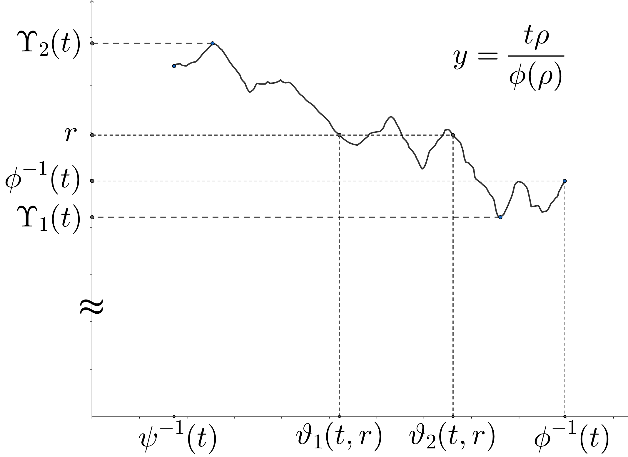
Figure 2. Auxiliary functions

Lemma 4.1.

For all $\varepsilon\in(0,1)$ and $t,r>0$ satisfying ${\Upsilon}_{1}(t)\leq\varepsilon r$, it holds that

$$\frac{\varepsilon r}{{\vartheta}_{1}(t,\varepsilon r)}\geq\frac{t}{\phi({\vartheta}_{1}(t,\varepsilon r))}.$$

Proof. If $\varepsilon r\leq{\Upsilon}_{2}(t)$, then $t{\vartheta}_{1}(t,\varepsilon r)/\phi({\vartheta}_{1}(t,\varepsilon r))\leq\varepsilon r$ and hence

$$\frac{r}{{\vartheta}_{1}(t,\varepsilon r)}-\frac{t}{\phi({\vartheta}_{1}(t,\varepsilon r))}=\frac{1}{{\vartheta}_{1}(t,\varepsilon r)}\Big{(}r-\frac{t{\vartheta}_{1}(t,\varepsilon r)}{\phi({\vartheta}_{1}(t,\varepsilon r))}\Big{)}\geq\frac{(1-\varepsilon)r}{{\vartheta}_{1}(t,\varepsilon r)}.$$

Otherwise, if $\varepsilon r>{\Upsilon}_{2}(t)$, then since $t{\vartheta}_{1}(t,\varepsilon r)/\phi({\vartheta}_{1}(t,\varepsilon r))\leq{\Upsilon}_{2}(t)$, we also obtain

$$\frac{r}{{\vartheta}_{1}(t,\varepsilon r)}-\frac{t}{\phi({\vartheta}_{1}(t,\varepsilon r))}=\frac{1}{{\vartheta}_{1}(t,\varepsilon r)}\Big{(}r-\frac{t{\vartheta}_{1}(t,\varepsilon r)}{\phi({\vartheta}_{1}(t,\varepsilon r))}\Big{)}\geq\frac{r-{\Upsilon}_{2}(t)}{{\vartheta}_{1}(t,\varepsilon r)}>\frac{(1-\varepsilon)r}{{\vartheta}_{1}(t,\varepsilon r)}.$$

$\Box$

The next lemma follows from the inequality $e^{-x}\leq\beta^{\beta}x^{-\beta}$, $x,\beta>0$.

Lemma 4.2.

(i) If ${\mathrm{US}}_{R_{0}}(\psi,\beta_{3},C_{U}^{\prime})$ holds, then for all $k>0$ and $0<\psi^{-1}(t)\leq r<R_{0}$,

$$\exp\left(-{kr}/{\psi^{-1}(t)}\right)\leq{C_{U}^{\prime}\beta_{3}^{\beta_{3}}k^{-\beta_{3}}t}/{\psi(r)}.$$ (4.5)

(ii) If ${\mathrm{US}}^{R_{\infty}}(\psi,\beta_{3},C_{U}^{\prime})$ holds, then (4.5) holds for all $k>0$ and $R_{\infty}<\psi^{-1}(t)\leq r$.

4.2. Estimates on the first exit times from open balls

In this subsection, we study the first exit time from open balls. The main results are Propositions 4.9 and 4.12. Note that a similar result appears in [3, (3.25)] (see also [19, (3.3)]). However, in this paper, we not only give local versions (in the variable $r$) of that result, but also remove an extra assumption that the local lower scaling index of $\phi$ is strictly larger than $1$ therein, by using auxiliary functions defined in subsection 4.1 and adopting the ideas from the first and second named authors’ paper [22, Theorem 3.10].

In the following proposition, we let $\ell>1$ be the constant in (1.4),

$$r_{0}:=\eta^{2}R_{0}/(6\ell)\;\;\text{with the constant $\eta\in(0,1)$ from ${\mathrm{NDL}}_{R_{0}}(\phi,U)$}$$ (4.6)

in the first statement, and

$$r_{\infty}:=(4\ell R_{\infty})^{1/(1-{\upsilon})}\vee(2R_{\infty}/\eta^{2})\;\;\text{with the constants ${\upsilon},\eta\in(0,1)$ from ${\mathrm{NDL}}^{R_{\infty}}(\phi)$}$$ (4.7)

in the latter statement. Note that $r_{0}=\infty$ if $R_{0}=\infty$.

Proposition 4.3.

(i) Suppose that ${\mathrm{VRD}}_{R_{0}}(U)$, ${\mathrm{NDL}}_{R_{0}}(\phi,U)$ and ${\mathrm{US}}_{R_{0}}(\phi,\beta_{2},C_{U})$ hold. Then there exist constants $C_{1}^{\prime},A_{0}^{\prime},a_{1},a_{2}>0$ such that for all $n\geq 1$, $x\in U$ and $0<r<r_{0}\land(C_{1}^{\prime}\updelta_{U}(x))$,

$$e^{-a_{1}n}\leq{\mathbb{P}}^{x}(\tau_{B(x,r)}\geq n\phi(A_{0}^{\prime}r))\leq e^{-a_{2}n}.$$ (4.8)

Moreover, $\mathrm{E}_{r_{0}}(\phi,U)$ holds.

(ii) Suppose that ${\mathrm{VRD}}^{R_{\infty}}$, ${\mathrm{NDL}}^{R_{\infty}}(\phi)$ and ${\mathrm{US}}^{R_{\infty}}(\phi,\beta_{2},C_{U})$ hold. Then there exist constants $A_{0}^{\prime},a_{1},a_{2}>0$ such that (4.8) holds for all $n\geq 1$, $x\in M$ and $r>r_{\infty}{\mathsf{d}}(x)^{\upsilon}$, and $\mathrm{E}^{r_{\infty}}(\phi)$ holds.

Proof. We adopt the idea from the proof for [20, Proposition 3.5(ii)].

(i) Let $C_{1}^{\prime}=\eta^{2}(C_{V}\land C_{2})/(5\ell)$ and $A_{0}^{\prime}=4\ell/\eta$, where $C_{V},C_{2},\eta\in(0,1)$ are the constants in ${\mathrm{VRD}}_{R_{0}}(U)$, ${\mathrm{NDL}}_{R_{0}}(\phi,U)$ and ${\mathrm{NDL}}_{R_{0}}(\phi,U)$, respetively, and $\ell>1$ is the constant in (1.4). Choose $x\in U$ and $0<r<r_{0}\land(C_{1}^{\prime}\updelta_{U}(x))$. Set $t_{r}:=\phi(3\ell\eta^{-1}r)$. Then $\phi^{-1}(t_{r})/\eta=3\ell r/\eta^{2}<R_{0}\land((C_{V}\land C_{2})\updelta_{U}(x))$. Thus, by ${\mathrm{NDL}}_{R_{0}}(\phi,U)$ and ${\mathrm{VRD}}_{R_{0}}(U)$, it hold that

$$p^{B(x,\phi^{-1}(t_{r})/\eta)}(t_{r},y,z)\geq\frac{c_{1}}{V(x,\phi^{-1}(t_{r})/\eta)}\geq\frac{c_{2}}{V(x,r)},\quad\;\;\forall\,y,z\in B(x,3\ell r).$$ (4.9)

Meanwhile, by (1.4), one can pick $w\in B(x,2\ell r)\setminus B(x,2r)$. Observe that $B(w,r)\cap B(x,r)=\emptyset$, $B(x,r)\subset B(w,3\ell r)$, $B(w,r)\subset B(x,3\ell r)$ and $\updelta_{U}(w)\geq\updelta_{U}(x)-2\ell r>(C_{1}^{\prime-1}-2\ell)r\geq 3C_{V}^{-1}\ell r$. By ${\mathrm{VRD}}_{R_{0}}(U)$, it follows that $V(w,r)\geq c_{3}V(w,3\ell r)\geq c_{3}V(x,r)$. Then by (4.9), it holds that

$${\mathbb{P}}^{y}\big{(}X_{t_{r}}\notin B(x,r)\big{)}\geq{\mathbb{P}}^{y}\big{(}X^{B(x,\phi^{-1}(t_{r})/\eta)}_{t_{r}}\in B(w,r)\big{)}\geq\frac{c_{2}V(w,r)}{V(x,r)}\geq c_{2}c_{3},\quad\forall\,y\in B(x,r).$$ (4.10)

Using the Markov property, we get from (4.10) that for all $n\geq 1$,

$${\mathbb{P}}^{x}\big{(}\tau_{B(x,r)}\geq n\phi(A_{0}^{\prime}r)\big{)} \leq{\mathbb{E}}^{x}\left[{\bf 1}_{\{\tau_{B(x,r)}\geq(n-1)\phi(A_{0}^{\prime}r)\}}{\mathbb{P}}^{X_{(n-1)\phi(A_{0}^{\prime}r)}}(\tau_{B(x,r)}\geq\phi(A_{0}^{\prime}r))\right]$$

$$\leq{\mathbb{P}}^{x}\big{(}\tau_{B(x,r)}\geq(n-1)\phi(A_{0}^{\prime}r)\big{)}\sup_{y\in B(x,r)}{\mathbb{P}}^{y}\big{(}\tau_{B(x,r)}\geq\phi(A_{0}^{\prime}r)\big{)}$$

$$\leq(1-c_{2}c_{3})\,{\mathbb{P}}^{x}\big{(}\tau_{B(x,r)}\geq(n-1)\phi(A_{0}^{\prime}r)\big{)}\leq\dots\leq(1-c_{2}c_{3})^{n}.$$ (4.11)

Next, we prove the lower bound in (4.8). Set $k:=\lceil C_{U}(A_{0}^{\prime}/\eta)^{\beta_{2}}\rceil$. Using ${\mathrm{US}}_{R_{0}}(\phi,\beta_{2},C_{U})$, the semigroup property and ${\mathrm{VRD}}_{R_{0}}(U)$, we get that for all $n\geq 1$,

$${\mathbb{P}}^{x}\big{(}\tau_{B(x,r)}\geq n\phi(A_{0}^{\prime}r)\big{)}\geq{\mathbb{P}}^{x}\big{(}\tau_{B(x,r)}\geq kn\phi(\eta r)\big{)}\geq\int_{B(x,\eta^{2}r)}p^{B(x,r)}(kn\phi(\eta r),x,z_{kn})\mu(dz_{kn})$$

$$\geq\int_{B(x,\eta^{2}r)}\dots\int_{B(x,\eta^{2}r)}p^{B(x,r)}(\phi(\eta r),x,z_{1})\dots p^{B(x,r)}(\phi(\eta r),z_{kn-1},z_{kn})\mu(dz_{1})\dots\mu(dz_{kn})$$

$$\geq\bigg{(}\frac{c_{4}}{V(x,r)}\bigg{)}^{kn}\int_{B(x,\eta^{2}r)}\dots\int_{B(x,\eta^{2}r)}\mu(dz_{1})\dots\mu(dz_{kn})=\bigg{(}\frac{c_{4}V(x,\eta^{2}r)}{V(x,r)}\bigg{)}^{kn}\geq e^{-c_{5}n}.$$ (4.12)

We have established (4.8). Now using Markov inequality, we get from (4.8) that

$${\mathbb{E}}^{x}[\tau_{B(x,r)}]\geq\phi(A_{0}^{\prime}r){\mathbb{P}}^{x}(\tau_{B(x,r)}\geq\phi(A_{0}^{\prime}r))\geq e^{-a_{1}}\phi(A_{0}^{\prime}r)$$ (4.13)

and

$${\mathbb{E}}^{x}[\tau_{B(x,r)}] \leq\sum_{n=1}^{\infty}n\phi(A_{0}^{\prime}r){\mathbb{P}}^{x}\big{(}\tau_{B(x,r)}\geq(n-1)\phi(A_{0}^{\prime}r)\big{)}$$

$$\leq\phi(A_{0}^{\prime}r)\sum_{n=1}^{\infty}ne^{-a_{2}(n-1)}=c_{6}\phi(A_{0}^{\prime}r).$$ (4.14)

Therefore, $\mathrm{E}_{r_{0}}(\phi,U)$ holds.

(ii) We follow the proof of (i). Choose any $x\in M$, $r>r_{\infty}{\mathsf{d}}(x)^{\upsilon}$ and let $t_{r}:=\phi(3\ell\eta^{-1}r)$. Since $\phi^{-1}(t_{r})/\eta=3\ell\eta^{-2}r>R_{\infty}{\mathsf{d}}(x)^{\upsilon}$, by ${\mathrm{NDL}}^{R_{\infty}}(\phi)$ and ${\mathrm{VRD}}^{R_{\infty}}$, (4.9) is still valid. Also, we can pick $w\in B(x,2\ell r)\setminus B(x,2r)$ by (1.4). Using the inequality $(a+b)^{\upsilon}\leq a^{\upsilon}+b^{\upsilon}$ for $a,b\geq 0$, we get

$$R_{\infty}{\mathsf{d}}(w)^{\upsilon}\leq R_{\infty}({\mathsf{d}}(x)+2\ell r)^{\upsilon}\leq R_{\infty}({\mathsf{d}}(x)^{\upsilon}+(2\ell r)^{\upsilon})<(2^{-1}+2\ell R_{\infty}r_{\infty}^{{\upsilon}-1})r\leq r.$$

Hence, we see from ${\mathrm{VRD}}^{R_{\infty}}$ that $V(w,r)\geq c_{1}V(w,3\ell r)\geq c_{1}V(x,r)$ and (4.10) is true. Using the Markov property again, we deduce that (4.2) holds. On the other hand, we can still get (4.2) from ${\mathrm{US}}^{R_{\infty}}(\phi,\beta_{2},C_{U})$ and ${\mathrm{NDL}}^{R_{\infty}}(\phi)$ since $\eta^{2}r_{\infty}>R_{\infty}$. Therefore, (4.8) is true. Now, we conclude that $\mathrm{E}^{r_{\infty}}(\phi)$ holds by (4.13) and (4.2). $\Box$

For sake of brevity, we give three families of conditions.

Assumption 4.4.

$\mathrm{E}_{R_{0}}(\phi,U)$, ${\mathrm{TJ}}_{R_{0}}(\phi,\leq,U)$ and ${\mathrm{US}}_{R_{0}}(\phi,\beta_{2},C_{U})$ hold (with $C_{1}$) for some $R_{0}\in(0,\infty]$ and an open set $U\subset M$.

Assumption 4.5.

$\mathrm{E}^{R_{\infty}}(\phi)$, ${\mathrm{TJ}}^{R_{\infty}}(\phi,\leq)$ and ${\mathrm{US}}^{R_{\infty}}(\phi,\beta_{2},C_{U})$ hold for some $R_{\infty}\geq 1$ and ${\upsilon}\in(0,1)$.

Assumption 4.6.

${\mathrm{VRD}}^{R_{\infty}}$, ${\mathrm{NDL}}^{R_{\infty}}(\phi)$, ${\mathrm{TJ}}^{R_{\infty}}(\phi,\leq)$, ${\mathrm{LS}}^{R_{\infty}}(\phi,\beta_{1},C_{L})$ and ${\mathrm{US}}^{R_{\infty}}(\phi,\beta_{2},C_{U})$ hold for some $R_{\infty}\geq 1$ and ${\upsilon}\in(0,1)$.

By Proposition 4.3(ii), Assumption 4.6 is stronger than Assumption 4.5. Assumption 4.6 will be used in the next subsection to establish estimates on oscillation of bounded parabolic functions and obtain a zero-one law.

For $\rho>0$, let $X^{(\rho)}$ be a Markov process on $M$ obtained by eliminating all jumps with absolute jump size bigger than $\rho$ from $X$. Then $X^{(\rho)}$ is a Borel standard Markov process on $M$ with the Lévy measure $J^{(\rho)}(x,dy):={\bf 1}_{B(x,\rho)}(y)J(x,dy)$. By the Meyer’s construction (see [52], and also [8, Section 3]), $X$ can be constructed from $X^{(\rho)}$ by attaching large jumps whose sizes are bigger than $\rho$. For an open set $D\subset M$, we denote $\tau^{(\rho)}_{D}:=\inf\{t>0:X^{(\rho)}_{t}\in M_{\partial}\setminus D\}$.

Our first goal is obtaining Proposition 4.9 below. For this, we prepare two lemmas. The main strategies of the proofs for the next two lemmas are similar to those for [17, Lemmas 4.20 and 4.21]. Under Assumption 4.5, for each ${\upsilon}_{1}\in({\upsilon},1)$, we define

$$R_{\infty}^{\prime}=R_{\infty}^{\prime}({\upsilon}_{1}):=(7R_{\infty})^{{\upsilon}_{1}/({\upsilon}-{\upsilon}{\upsilon}_{1})}.$$ (4.15)

Lemma 4.7.

(i) Suppose that Assumption 4.4 holds. Then, there exist constants $\delta\in(0,1)$ and $C_{3}\geq 1$ such that for all $x\in U$, $0<\rho\leq r<3^{-1}\big{(}R_{0}\land(C_{1}\updelta_{U}(x))\big{)}$ and $\lambda\geq C_{3}/\phi(\rho)$,

$${\mathbb{E}}^{x}\left[\exp\big{(}-\lambda\tau^{(\rho)}_{B(x,r)}\big{)}\right]\leq 1-\delta.$$ (4.16)

(ii) Suppose that Assumption 4.5 holds. Then, there exist constants $\delta\in(0,1)$ and $C_{3}\geq 1$ such that (4.16) holds for any ${\upsilon}_{1}\in({\upsilon},1)$, $x_{0}\in M$, $r>R_{\infty}^{\prime}{\mathsf{d}}(x_{0})^{{\upsilon}_{1}}$, $x\in B(x_{0},6r)$, $2r^{{\upsilon}/{\upsilon}_{1}}\leq\rho\leq r$ and $\lambda\geq C_{3}/\phi(\rho)$, where $R_{\infty}^{\prime}=R_{\infty}^{\prime}({\upsilon}_{1})$ is defined by (4.15).

Proof. (i) Choose any $x\in U$ and $0<r<3^{-1}\big{(}R_{0}\land(C_{1}\updelta_{U}(x))\big{)}$. Set $B:=B(x,r)$. Then we have

$$C_{1}\updelta_{U}(z)\geq C_{1}(\updelta_{U}(x)-r)>2r\quad\text{for all}\;\;z\in B.$$ (4.17)

Hence, since $\mathrm{E}_{R_{0}}(\phi,U)$ holds, by using the inequality $\tau_{B}\leq t+(\tau_{B}-t)1_{\{\tau_{B}>t\}}$ and the Markov property, we get that for all $t>0$,

$$c_{1}\phi(r) \leq{\mathbb{E}}^{x}\tau_{B}\leq t+{\mathbb{E}}^{x}\left[{\bf 1}_{\{\tau_{B}>t\}}{\mathbb{E}}^{X_{t}}\tau_{B}\right]\leq t+{\mathbb{P}}^{x}(\tau_{B}>t)\sup_{z\in B}{\mathbb{E}}^{z}\tau_{B}$$

$$\leq t+{\mathbb{P}}^{x}(\tau_{B}>t)\sup_{z\in B}{\mathbb{E}}^{z}\tau_{B(z,2r)}\leq t+c_{2}{\mathbb{P}}^{x}(\tau_{B}>t)\phi(2A_{0}r).$$

Since ${\mathrm{US}}_{R_{0}}(\phi,\beta_{2},C_{U})$ holds and $\phi$ is increasing, it follows that

$${\mathbb{P}}^{x}(\tau_{B}>t)\geq\frac{c_{1}\phi(r)}{c_{2}\phi(2A_{0}r)}-\frac{t}{c_{2}\phi(2A_{0}r)}\geq c_{3}-\frac{t}{c_{3}\phi(r)}\quad\text{for all}\;\;t>0,$$ (4.18)

for some constant $c_{3}\in(0,1)$. We claim that there exists a constant $c_{4}>0$ independent of $x$ and $r$ such that

$$\Big{|}{\mathbb{P}}^{x}\big{(}\tau_{B}>t\big{)}-{\mathbb{P}}^{x}\big{(}\tau_{B}^{(\rho)}>t\big{)}\Big{|}\leq\frac{c_{4}t}{\phi(\rho)}\quad\;\;\text{ for all}\;\;\rho\in(0,r],\;\;t>0.$$ (4.19)

To prove (4.19), we need some preparations. Choose any $\rho\in(0,r]$. Let $\xi$ be an exponential random variable with rate parameter $1$ independent of $X^{(\rho)}$. Define ${\cal J}_{t}:=\int_{0}^{t}J\big{(}X_{s}^{(\rho)},M_{\partial}\setminus B(X_{s}^{(\rho)},\rho)\big{)}ds$ and $T_{0}:=\inf\{t\geq 0:{\cal J}_{t}\geq\xi\}$. In view of the Meyer’s construction, we may identify $T_{0}$ with $T_{1}:=\inf\{t>0:X_{t}\neq X^{(\rho)}_{t}\}$, the first attached jump time for $X^{(\rho)}$ (see [8, Section 3.1]). Since $\mathrm{TJ}_{R_{0}}(\phi,\leq,U)$ holds and $X_{s}^{(\rho)}\in B$ for all $0\leq s<t\land\tau_{B}^{(\rho)}$, by (4.17), we have that

$${\mathbb{P}}^{x}\big{(}T_{1}\leq t\land\tau_{B}^{(\rho)}\big{)}={\mathbb{P}}^{x}\big{(}{\cal J}_{t\land\tau_{B}^{(\rho)}}\geq\xi\big{)}\leq{\mathbb{P}}^{x}\big{(}\frac{c_{5}t}{\phi(\rho)}\geq\xi\big{)}\leq\frac{c_{5}t}{\phi(\rho)}.$$ (4.20)

Besides, since $X_{s}=X^{(\rho)}_{s}$ for $s<T_{1}$, we have $\{t<T_{1}\land\tau_{B}\}=\{t<T_{1}\land\tau^{(\rho)}_{B}\}$ and $\{T_{1}\leq t<\tau_{B}\}\subset\{T_{1}\leq t\land\tau^{(\rho)}_{B}\}$ for all $t>0$. Thus, we can see from (4.20) that for all $t>0$,

$$\Big{|}{\mathbb{P}}^{x}\big{(}t<\tau_{B}\big{)}-{\mathbb{P}}^{x}\big{(}t<\tau_{B}^{(\rho)}\big{)}\Big{|}=\Big{|}{\mathbb{P}}^{x}\big{(}T_{1}\leq t<\tau_{B}\big{)}-{\mathbb{P}}^{x}\big{(}T_{1}\leq t<\tau_{B}^{(\rho)}\big{)}\Big{|}$$

$$\leq{\mathbb{P}}^{x}\big{(}T_{1}\leq t<\tau_{B}\big{)}+{\mathbb{P}}^{x}\big{(}T_{1}\leq t<\tau_{B}^{(\rho)}\big{)}\leq 2\,{\mathbb{P}}^{x}\big{(}T_{1}\leq t\land\tau_{B}^{(\rho)}\big{)}\leq\frac{2c_{5}t}{\phi(\rho)}.$$

This yields (4.19) with $c_{4}=2c_{5}$.

Now, set $\delta=c_{3}/3\in(0,1/3)$ and $C_{3}=(c_{3}^{-1}+c_{4})\delta^{-1}\log(\delta^{-1})$. In view of (4.18) and (4.19), by taking $t_{\rho}=\delta\phi(\rho)/(c_{3}^{-1}+c_{4})$, we conclude that for all $\rho\in(0,r]$ and $\lambda\geq C_{3}/\phi(\rho)$,

$${\mathbb{E}}^{x}\left[\exp\big{(}-\lambda\tau_{B}^{(\rho)}\big{)}\right] \leq{\mathbb{E}}^{x}\left[\exp\big{(}-\lambda\tau_{B}^{(\rho)}\big{)};\tau_{B}^{(\rho)}\leq t_{\rho}\right]+e^{-\lambda t_{\rho}}\leq{\mathbb{P}}^{x}(\tau_{B}^{(\rho)}\leq t_{\rho})+e^{-\lambda t_{\rho}}$$

$$\leq 1-c_{3}+\frac{(c_{3}^{-1}+c_{4})t_{\rho}}{\phi(\rho)}+\exp\Big{(}-\frac{C_{3}t_{\rho}}{\phi(\rho)}\Big{)}\leq 1-c_{3}+2\delta\leq 1-\delta.$$ (4.21)

Since $\delta$ and $C_{3}$ are independent of $x$ and $r$, this completes the proof.

(ii) Choose any $x_{0}\in M$, $r>R_{\infty}^{\prime}{\mathsf{d}}(x_{0})^{{\upsilon}_{1}}$, $x\in B(x_{0},6r)$ and $2r^{{\upsilon}/{\upsilon}_{1}}\leq\rho\leq r$. By (4.15), it holds that for any $z\in B(x,r)\subset B(x_{0},7r)$,

$$R_{\infty}{\mathsf{d}}(z)^{\upsilon}\leq R_{\infty}{\mathsf{d}}(x_{0})^{\upsilon}+(7r)^{\upsilon}R_{\infty}<(R_{\infty}R_{\infty}^{\prime-{\upsilon}/{\upsilon}_{1}}+7^{\upsilon}R_{\infty}R_{\infty}^{\prime\,{\upsilon}-{\upsilon}/{\upsilon}_{1}})r^{{\upsilon}/{\upsilon}_{1}}<2r^{{\upsilon}/{\upsilon}_{1}}\leq\rho.$$ (4.22)

Hence, since $\mathrm{E}^{R_{\infty}}(\phi)$, $\mathrm{TJ}^{R_{\infty}}(\phi,\leq)$ and ${\mathrm{US}}^{R_{\infty}}(\phi,\beta_{2},C_{U})$ hold, we see that (4.18) and (4.19) hold by following the proof for (i). By repeating the calculations (4.2), we obtain the result. $\Box$

Lemma 4.8.

(i) Suppose that Assumption 4.4 holds. Then there exist constants $C_{4}>0$, $C_{5}\in(0,1]$ such that for all $x\in U$ and $0<\rho\leq r<3^{-1}\big{(}R_{0}\land(C_{1}\updelta_{U}(x))\big{)}$,

$${\mathbb{E}}^{x}\bigg{[}\exp\Big{(}-\frac{C_{3}}{\phi(\rho)}\tau_{B(x,r)}^{(\rho)}\Big{)}\bigg{]}\leq C_{4}\exp\big{(}-C_{5}\frac{r}{\rho}\big{)},$$ (4.23)

where $C_{3}$ is the constant in Lemma 4.7(i).

(ii) Suppose that Assumption 4.5 holds. Then there exist constants $C_{4}>0$, $C_{5}\in(0,1]$ such that (4.23) holds for any ${\upsilon}_{1}\in({\upsilon},1)$, $x_{0}\in M$, $r>R_{\infty}^{\prime}{\mathsf{d}}(x_{0})^{{\upsilon}_{1}}$, $x\in B(x_{0},5r)$ and $2r^{{\upsilon}/{\upsilon}_{1}}\leq\rho\leq r$ where $C_{3}$ is the constant in Lemma 4.7(ii) and $R_{\infty}^{\prime}$ is defined by (4.15).

Proof. (i) Choose any $x\in U$ and $0<\rho\leq r<3^{-1}\big{(}R_{0}\land(C_{1}\updelta_{U}(x))\big{)}$. If $6\rho>r$, then by taking $C_{4}$ larger than $e^{6}$, we are done. Hence, we assume that $6\rho\leq r$.

Set $\lambda_{\rho}:=C_{3}/\phi(\rho)$, $n_{\rho}:=\lceil r/(6\rho)\rceil$, $\tau_{0}:=\tau^{(\rho)}_{B(x,r)}$, $u(y):={\mathbb{E}}^{y}[e^{-\lambda_{\rho}\tau_{0}}]$ and $m_{k}:=\|u\|_{L^{\infty}(\overline{B(x,k\rho)};\mu)}$. Let $\delta\in(0,1)$ be the constant in Lemma 4.7(i). Fix any $\delta^{\prime}\in(0,\delta)$. Then for each $1\leq k\leq 2n_{\rho}$, choose any $x_{k}\in\overline{B(x,k\rho)}$ such that $(1-\delta^{\prime})m_{k}\leq u(x_{k})\leq m_{k}$. Since $(2n_{\rho}+2)\rho<r/3+4\rho\leq r$, we see that $B(x_{k},2\rho)\subset B(x,(k+2)\rho)\subset B(x,r)$ for all $1\leq k\leq 2n_{\rho}$.

Set $\tau_{k}:=\tau^{(\rho)}_{B(x_{k},\rho)}$ and $v_{k}(y):={\mathbb{E}}^{y}[e^{-\lambda_{\rho}\tau_{k}}]$. Note that $3^{-1}C_{1}\updelta_{U}(y)>3^{-1}C_{1}(\updelta_{U}(x)-r)>3^{-1}r\geq\rho$ for all $y\in B(x,r)$. Hence, by Lemma 4.7(i), we obtain $v_{k}(x_{k})\leq 1-\delta$. Then by the strong Markov property, it holds that for all $1\leq k\leq 2n_{\rho}-2$,

$$(1-\delta^{\prime})m_{k}\leq u(x_{k}) ={\mathbb{E}}^{x_{k}}\big{[}e^{-\lambda_{\rho}\tau_{0}}\,;\,\tau_{k}\leq\tau_{0}<\infty\big{]}={\mathbb{E}}^{x_{k}}\big{[}e^{-\lambda_{\rho}\tau_{k}}e^{-\lambda_{\rho}(\tau_{0}-\tau_{k})}\,;\,\tau_{k}\leq\tau_{0}<\infty\big{]}$$

$$={\mathbb{E}}^{x_{k}}\big{[}e^{-\lambda_{\rho}\tau_{k}}{\mathbb{E}}^{X^{(\rho)}_{\tau_{k}}}(e^{-\lambda_{\rho}\tau_{0}})\big{]}={\mathbb{E}}^{x_{k}}\big{[}e^{-\lambda_{\rho}\tau_{k}}u(X_{\tau_{k}}^{(\rho)})\big{]}$$

$$\leq v_{k}(x_{k})\|u\|_{L^{\infty}(\overline{B(x_{k},2\rho)};\mu)}\leq v_{k}(x_{k})m_{k+2}\leq(1-\delta)m_{k+2}.$$ (4.24)

In the first inequality above, we used the fact that $X^{(\rho)}_{\tau_{k}}\in\overline{B(x_{k},2\rho)}$ since the jump size of $X^{(\rho)}$ can not be larger than $\rho$. The second inequality above holds since $B(x_{k},2\rho)\subset B(x,(k+2)\rho)$.

In the end, by (4.2), we conclude that

$${\mathbb{E}}^{x}\Big{[}\exp\Big{(}-\frac{C_{3}}{\phi(\rho)}\tau_{B(x,r)}^{(\rho)}\Big{)}\Big{]}=u(x)\leq m_{1}\leq\Big{(}\frac{1-\delta}{1-\delta^{\prime}}\Big{)}^{n_{\rho}-1}m_{2n_{\rho}-1}\leq\frac{1-\delta^{\prime}}{1-\delta}\exp\Big{(}-\frac{r}{6\rho}\log\frac{1-\delta^{\prime}}{1-\delta}\Big{)}.$$

In the last inequality above, we used the fact that $m_{2n_{\rho}-1}\leq\|u\|_{L^{\infty}(M;\mu)}\leq 1$. This proves (4.23).

(ii) By following the proof for (i), using Lemma 4.7(ii), one can obtain (4.23). Note that since $x\in B(x_{0},5r)$, the point $x_{k}$ in (4.2) satisfies $x_{k}\in B(x,k\rho)\subset B(x_{0},6r)$ so that we can apply Lemma 4.7(ii) in the counterpart of (4.2). $\Box$

Recall that ${\Upsilon}_{1},{\Upsilon}_{2},{\vartheta}_{1}$ and ${\vartheta}_{2}$ are auxiliary functions discussed in Subsection 4.1.

Proposition 4.9.

(i) Suppose that Assumption 4.4 holds. Then, there exists a constant $C_{6}\geq 1$ such that for all $x\in U$, $0<r<3^{-1}\big{(}R_{0}\land(C_{1}\updelta_{U}(x))\big{)}$ and $t>0$,

$${\mathbb{P}}^{x}(\tau_{B(x,r)}\leq t)\leq\frac{C_{6}t}{\phi(r)}.$$ (4.25)

If ${\mathrm{TJ}}_{R_{0}}(\psi,\leq,U)$ and ${\mathrm{US}}_{R_{0}}(\psi,\beta_{3},C_{U}^{\prime})$ also hold, then there exist constants $C_{7},C_{8},C_{9}>0$ such that for all $x\in U$, $0<r<3^{-1}(R_{0}\land(C_{1}\updelta_{U}(x)))$ and $t>0$,

$${\mathbb{P}}^{x}(\tau_{B(x,r)}\leq t)\leq C_{7}\bigg{(}\frac{t}{\psi(r)}+\exp\Big{(}-\frac{C_{8}r}{{\vartheta}_{1}(t,C_{9}r)}\Big{)}\bigg{)}$$ (4.26)

(ii) Suppose that Assumption 4.5 holds. Then, there exists a constant $C_{6}\geq 1$ such that (4.25) holds for any ${\upsilon}_{1}\in({\upsilon},1)$, $x\in M$, $r>R_{\infty}^{\prime}{\mathsf{d}}(x)^{{\upsilon}_{1}}$ and $t\geq\phi(2r^{{\upsilon}/{\upsilon}_{1}})$ where $R_{\infty}^{\prime}$ is defined by (4.15). If $\mathrm{TJ}^{R_{\infty}}(\psi,\leq)$ and ${\mathrm{US}}^{R_{\infty}}(\psi,\beta_{3},C_{U}^{\prime})$ also hold, then there exist constants $C_{7},C_{8},C_{9}>0$ such that (4.26) holds for all $x\in M$, $r>R_{\infty}^{\prime}{\mathsf{d}}(x)^{{\upsilon}_{1}}$ and $t\geq\psi(2r^{{\upsilon}/{\upsilon}_{1}})$.

Proof. (i) First, assuming that (4.26) holds under the further assumptions ${\mathrm{TJ}}_{R_{0}}(\psi,\leq,U)$ and ${\mathrm{US}}_{R_{0}}(\psi,\beta_{3},C_{U}^{\prime})$ for the moment. Then since $\mathrm{TJ}_{R_{0}}(\phi,\leq,U)$ and ${\mathrm{US}}_{R_{0}}(\phi,\beta_{2},C_{U})$ are contained in Assumption 4.4, we deduce that under Assumption 4.4 only, for all $x\in U$, $0<r<3^{-1}\big{(}R_{0}\land(C_{1}\updelta_{U}(x))\big{)}$ and $t\in(0,\phi(r)]$, since ${\vartheta}_{1}(t,C_{9}r)\leq\phi^{-1}(t)$ and ${\mathrm{US}}_{R_{0}}(\phi,\beta_{2},C_{U})$ holds, by (4.5),

$${\mathbb{P}}^{x}(\tau_{B}\leq t)\leq C_{7}\bigg{(}\frac{t}{\phi(r)}+\exp\Big{(}-\frac{C_{8}r}{\phi^{-1}(t)}\Big{)}\bigg{)}\leq\frac{(C_{7}+\beta_{2}^{\beta_{2}}C_{U}C_{8}^{-\beta_{2}})t}{\phi(r)}.$$

Hence, we obtain (4.25) (since it holds trivially in case $t>\phi(r)$). Therefore, it suffices to prove (4.26) under the further assumptions ${\mathrm{TJ}}_{R_{0}}(\psi,\leq,U)$ and ${\mathrm{US}}_{R_{0}}(\psi,\beta_{3},C_{U}^{\prime})$.

Now, we prove (4.26). Choose any $x\in U$, $0<r<3^{-1}\big{(}R_{0}\land(C_{1}\updelta_{U}(x))\big{)}$ and $t>0$. Set $B:=B(x,r)$ and let $C_{3},C_{4},C_{5}$ be the constants in Lemmas 4.7(i) and 4.8(i). Let $C_{9}=C_{5}/(8C_{3})$. If ${\vartheta}_{1}(t,C_{9}r)\geq r/4$, then by taking $C_{7}$ larger than $e^{4C_{8}}$, we obtain (4.26). Besides, if $C_{9}r<{\Upsilon}_{1}(t)$, then by (4.2) and (4.3), it holds $\exp\big{(}-C_{8}r/{\vartheta}_{1}(t,C_{9}r)\big{)}\geq\exp\big{(}-C_{8}C_{9}^{-1}\big{)}$. Thus, by taking $C_{7}$ larger than $e^{C_{8}/C_{9}}$, we get (4.26). Therefore, we suppose that ${\vartheta}_{1}(t,C_{9}r)<r/4$ and $C_{9}r\geq{\Upsilon}_{1}(t)$.

Let $\rho\in[\psi^{-1}(t),r/4)$ be a constant chosen later. Let $Y^{1}:=X^{(\rho)}$ be a $\rho$-truncated process. Recall that the Lévy measure of $Y^{1}$ is given by $J_{0}(x,dy):=J(x,dy){\bf 1}_{\{|x-y|<\rho\}}$. Set

$$J_{1}(x,dy):=J(x,dy){\bf 1}_{\{\rho\leq|x-y|<r/4\}}\quad\text{and}\quad J_{2}(x,dy){\bf 1}_{\{|x-y|\geq r/4\}}.$$

Let $(\xi^{1}_{n})_{n\geq 1}$ be i.i.d. exponential random variables with rate parameter $1$ independent of $Y^{1}$, and define an additive functional of $Y^{1}$ as

$$H_{1,u}:=\int_{0}^{u}J_{1}(Y^{1}_{s},M_{\partial})ds.$$ (4.27)

Set $S_{1,1}=\inf\{u>0:H_{1,u}\geq\xi_{1}^{1}\}$. Let $Y^{2}_{s}=Y^{1}_{s}$ for $0\leq s<S_{1,1}$, and then define $Y^{2}_{S_{1,1}}$ with law $J_{1}(Y^{2}_{S_{1,1}-},\cdot)/J_{1}(Y^{2}_{S_{1,1}-},M_{\partial})$. Repeat this procedure with the new starting point $(S_{1,1},Y^{2}_{S_{1,1}})$ to determine the next random time $S_{1,2}:=\inf\{u>0:H_{1,u}\circ\theta^{Y^{2}}_{S_{1,1}}\geq\xi_{2}^{1}\}$, where $\theta^{Y^{2}}$ denotes the shift operator with respect to $Y^{2}$, and behaviors of $Y^{2}_{u}$ for $u\in(S_{1,1},S_{1,1}+S_{1,2}]$. Let $T_{1,0}=0$ and $T_{1,n}:=\sum_{k=1}^{n}S_{1,k}$ for $n\geq 1$. By iterating this procedure, one can construct a process $Y^{2}_{u}$ for $u\in[0,\,\lim_{n\to\infty}T_{1,n}]\cap[0,\infty)$. Next, by setting $Y^{2}$ as the new underlying process, using the additive functional (of $Y^{2}$)

$$H_{2,u}:=\int_{0}^{u}J_{2}(Y^{2}_{s},M_{\partial})ds$$ (4.28)

and i.i.d. exponential random variables $(\xi^{2}_{n})_{n\geq 1}$ with rate parameter $1$ independent with all of $Y^{1},Y^{2}$ and $(\xi^{1}_{n})_{n\geq 1}$, one can construct a process $Y^{3}$, $S_{2,n}$ and $T_{2,n}$ by the same way. According to [52] (see also [8, Section 3.1]), the joint law of $\big{(}(Y^{2}_{u},Y^{3}_{u}):u\in[0,\,\lim_{n\to\infty}(T_{1,n}\wedge T_{2,n})\big{)}$ is the same as the one for $\big{(}(X^{(r/4)}_{u},X_{u}):u\in[0,\,\lim_{n\to\infty}(T_{1,n}\wedge T_{2,n})\big{)}$.

We note that $C_{1}\updelta_{U}(z)\geq C_{1}(\updelta_{U}(x)-r)\geq 2r$ for all $z\in B$. Thus, since ${\mathrm{TJ}}_{R_{0}}(\psi,\leq,U)$ and ${\mathrm{US}}_{R_{0}}(\psi,\beta_{3},C_{U}^{\prime})$ hold, we have that

$$\sup_{z\in B}J_{1}(z,M_{\partial})\leq\sup_{z\in B}J\big{(}z,M_{\partial}\setminus B(z,\rho)\big{)}\leq\frac{c_{1}}{\psi(\rho)},$$ (4.29)

$$\sup_{z\in B}J_{2}(z,M_{\partial})\leq\sup_{z\in U}J\big{(}z,M_{\partial}\setminus B(z,r/4)\big{)}\leq\frac{c_{1}}{\psi(r/4)}\leq\frac{4^{\beta_{3}}c_{1}C_{U}^{\prime}}{\psi(r)}=:\frac{c_{2}}{\psi(r)}.$$ (4.30)

Let $\widetilde{\tau}_{B}:=\inf\{u>0:Y^{3}_{u}\in M_{\partial}\setminus B\}$. In $[0,\widetilde{\tau}_{B})$, almost surely, there can be only finitely many extra jumps added in the construction of $Y^{3}$ from $Y^{1}$. Thus, for all $x\in U$, $\lim_{n\to\infty}(T_{1,n}\wedge T_{2,n})\geq\widetilde{\tau}_{B}$ (a.s.) under ${\mathbb{P}}^{x}$, and hence ${\mathbb{P}}^{x}(\tau_{B}\leq t)={\mathbb{P}}^{x}(\widetilde{\tau}_{B}\leq t)$. Therefore, we have

$${\mathbb{P}}^{x}(\tau_{B}\leq t) ={\mathbb{P}}^{x}(T_{2,1}\leq\widetilde{\tau}_{B}\leq t)+{\mathbb{P}}^{x}(T_{1,2}\leq\widetilde{\tau}_{B}\leq t,\,\widetilde{\tau}_{B}<T_{2,1})+{\mathbb{P}}^{x}(\widetilde{\tau}_{B}\leq t,\,\widetilde{\tau}_{B}<T_{1,2}\land T_{2,1})$$

$$=:P_{1}+P_{2}+P_{3}.$$ (4.31)

First, by (4.28) and (4.30), since $Y^{2}_{s}=Y^{3}_{s}\in B$ for all $s\in[0,T_{2,1}\wedge\widetilde{\tau}_{B})$, we have that

$$P_{1}={\mathbb{P}}^{x}\big{(}H_{2,S_{2,1}}\geq\xi^{2}_{1},\,S_{2,1}\leq\widetilde{\tau}_{B}\leq t\big{)}\leq{\mathbb{P}}^{x}\big{(}\frac{c_{2}S_{2,1}}{\psi(r)}\geq\xi^{2}_{1},\,S_{2,1}\leq t\big{)}\leq{\mathbb{P}}^{x}\big{(}\frac{c_{2}t}{\psi(r)}\geq\xi^{2}_{1}\big{)}\leq\frac{c_{2}t}{\psi(r)}.$$ (4.32)

Next, by a similar way, we get from (4.27) and (4.29) that

$$\begin{split}P_{2}&\leq{\mathbb{P}}^{x}\big{(}H_{1,S_{1,1}}+H_{1,S_{1,2}}\circ\theta^{Y^{2}}_{S_{1,1}}\geq\sum_{k=1}^{2}\xi_{k}^{1},\;\;S_{1,1}+S_{1,2}\leq\widetilde{\tau}_{B}\leq t,\,\widetilde{\tau}_{B}<S_{2,1}\big{)}\\ &\leq{\mathbb{P}}^{x}\big{(}\frac{c_{1}t}{\psi(\rho)}\geq\sum_{k=1}^{2}\xi_{k}^{1}\big{)}=\int_{0}^{c_{1}t/\psi(\rho)}le^{-l}dl\leq\Big{(}\frac{c_{1}t}{\psi(\rho)}\Big{)}^{2}.\end{split}$$ (4.33)

Lastly, we bound $P_{3}$. To do this, we set

$$g_{k}:=\sup\Big{\{}d(Y^{3}_{\widetilde{\tau}_{B}\land T_{1,k-1}},Y^{3}_{u-}):u\in(\widetilde{\tau}_{B}\land T_{1,k-1},\,\widetilde{\tau}_{B}\land T_{1,k}]\,\Big{\}},\quad k=1,2.$$

Note that on the event $\{\widetilde{\tau}_{B}\leq t,\,\widetilde{\tau}_{B}<T_{1,2}\wedge T_{2,1}\}$, by the triangle inequality, it holds that

$$r\leq d(x,Y^{3}_{\widetilde{\tau}_{B}}) \leq d(Y^{3}_{T_{1,0}},Y^{3}_{\widetilde{\tau}_{B}\land T_{1,1}-})+d(Y^{3}_{\widetilde{\tau}_{B}\land T_{1,1}-},Y^{3}_{\widetilde{\tau}_{B}\land T_{1,1}})+d(Y^{3}_{\widetilde{\tau}_{B}\land T_{1,1}},Y^{3}_{\widetilde{\tau}_{B}})\leq g_{1}+r/4+g_{2},$$

where in the third inequality above, we used the fact that the jump size at time $T_{1,1}-$ can not be larger than $r/4$ by the definition of $J_{1}$, and $\widetilde{\tau}_{B}=\widetilde{\tau}_{B}\land T_{1,2}$ on the event $\{\widetilde{\tau}_{B}\leq t,\,\widetilde{\tau}_{B}<T_{1,2}\land T_{2,1}\}$. Thus, we see that on the event $\{\widetilde{\tau}_{B}\leq t,\,\widetilde{\tau}_{B}<T_{1,2}\wedge T_{2,1}\}$,

$$\max\{g_{1},g_{2}\}>r/4,\quad\;\;{\mathbb{P}}^{x}\text{-a.s.}$$ (4.34)

Besides, since $3^{-1}C_{1}\updelta_{U}(z)\geq 3^{-1}C_{1}(\updelta_{U}(x)-5r/4)>r/4$ for all $z\in B(x,5r/4)$, according to Markov inequality and Lemma 4.8(i) we have that,

$$\sup_{z\in B(x,5r/4)}{\mathbb{P}}^{z}(\tau_{B(z,r/4)}^{(\rho)}\leq t)=\sup_{z\in B(x,5r/4)}{\mathbb{P}}^{z}\Big{(}\exp\big{(}-C_{3}\tau_{B(z,r/4)}^{(\rho)}/\phi(\rho)\big{)}\geq\exp\big{(}-C_{3}t/\phi(\rho)\big{)}\Big{)}$$

$$\leq\exp\big{(}C_{3}t/\phi(\rho)\big{)}\sup_{z\in B(x,5r/4)}{\mathbb{E}}^{z}\Big{[}\exp\big{(}-C_{3}\tau_{B(z,r/4)}^{(\rho)}/\phi(\rho)\big{)}\Big{]}\leq C_{4}\exp\big{(}-\frac{C_{5}r}{4\rho}+\frac{C_{3}t}{\phi(\rho)}\big{)}.$$ (4.35)

In view of the Meyer’s construction, on the event $\{\widetilde{\tau}_{B}\leq t,\,\widetilde{\tau}_{B}<T_{1,2}\land T_{2,1}\}$, for each $k=1,2$, the law of $\big{(}Y^{3}_{u}:u\in[\widetilde{\tau}_{B}\land T_{1,k-1},\widetilde{\tau}_{B}\land T_{1,k})\big{)}$ is the same as the one for $\big{(}Y^{1}_{u}:u\in[0,\widetilde{\tau}_{B}\land T_{1,k}-\widetilde{\tau}_{B}\land T_{1,k-1})\big{)}$ starting from $Y^{3}_{\widetilde{\tau}_{B}\land T_{1,k-1}}$. Therefore, by (4.34), (4.2) and the strong Markov property, we obtain

$$P_{3} ={\mathbb{P}}^{x}\big{(}\max\{g_{1},g_{2}\}>r/4,\;\widetilde{\tau}_{B}\leq t,\;\widetilde{\tau}_{B}<T_{1,2}\land T_{2,1}\big{)}$$

$$\leq{\mathbb{P}}^{x}\big{(}\min_{1\leq k\leq 2}\tau^{(\rho)}_{B(Y^{3}_{\widetilde{\tau}_{B}\land T_{1,k-1}},r/4)}\circ\theta^{Y^{3}}_{\widetilde{\tau}_{B}\land T_{1,k-1}}\leq t,\;\widetilde{\tau}_{B}\leq t,\;\widetilde{\tau}_{B}<T_{1,2}\land T_{2,1}\big{)}$$

$$\leq 2\sup_{z\in B(x,5r/4)}{\mathbb{P}}^{z}\big{(}\tau^{(\rho)}_{B(z,r/4)}\leq t\big{)}\leq 2C_{4}\exp\Big{(}-\frac{C_{5}r}{4\rho}+\frac{C_{3}t}{\phi(\rho)}\Big{)},$$ (4.36)

where $\theta^{Y^{3}}$ denotes the shift operator with respect to $Y^{3}$. In the second inequality above, we used the the fact that $Y^{3}_{\widetilde{\tau}_{B}\land T_{1,k-1}}\in B(x,r+r/4)$ for each $k=1,2$.

Eventually, by combining all of (4.2), (4.32), (4.33) and (4.2), we conclude that

$${\mathbb{P}}^{x}(\tau_{B}\leq t)\leq\frac{c_{2}t}{\psi(r)}+\Big{(}\frac{c_{1}t}{\psi(\rho)}\Big{)}^{2}+2C_{4}\exp\Big{(}-\frac{C_{5}r}{4\rho}+\frac{C_{3}t}{\phi(\rho)}\Big{)}.$$ (4.37)

For the last step of the proof, we first assume $t\psi(r/4)\leq\psi(\phi^{-1}(t))^{2}$. Then by Lemma 4.1, we see

$$\frac{C_{3}t}{\phi({\vartheta}_{1}(t,C_{9}r))}\leq\frac{C_{3}C_{9}r}{{\vartheta}_{1}(t,C_{9}r)}=\frac{C_{5}r}{8{\vartheta}_{1}(t,C_{9}r)}.$$

Further, since ${\mathrm{US}}_{R_{0}}(\psi,\beta_{3},C_{U}^{\prime})$ holds,

$$\Big{(}\frac{t}{\psi({\vartheta}_{1}(t,C_{9}r))}\Big{)}^{2}\leq\Big{(}\frac{t}{\psi(\phi^{-1}(t))}\Big{)}^{2}\leq\frac{t}{\psi(r/4)}\leq\frac{C_{U}^{\prime}4^{\beta_{3}}t}{\psi(r)}.$$

Thus, we get (4.26) by substituting $\rho={\vartheta}_{1}(t,C_{9}r)\in[\psi^{-1}(t),r/4)$ in (4.37).

Otherwise, if $t\psi(r/4)>\psi(\phi^{-1}(t))^{2}$, then we substitute $\rho=\psi^{-1}(t^{1/2}\psi(r/4)^{1/2})\in(\phi^{-1}(t),r/4)$ in (4.37). Since ${\mathrm{US}}_{R_{0}}(\psi,\beta_{3},C_{U}^{\prime})$ holds, we have $(t/\psi(\rho))^{2}=t/\psi(r/4)\leq C_{U}^{\prime}4^{\beta_{3}}t/\psi(r)$ and

$$\exp\big{(}-\frac{C_{5}r}{4\rho}+\frac{C_{3}t}{\phi(\rho)}\big{)}\leq e^{C_{3}}(2\beta_{3}/C_{5})^{2\beta_{3}}\Big{(}\frac{\rho}{r/4}\Big{)}^{2\beta_{3}}\leq c_{3}\Big{(}\frac{\psi(\rho)}{\psi(r/4)}\Big{)}^{2}=\frac{c_{3}t}{\psi(r/4)}\leq\frac{c_{4}t}{\psi(r)}.$$

In the first inequality above, we used the fact that $e^{-x}\leq(2\beta_{3})^{2\beta_{3}}x^{-2\beta_{3}}$ for all $x>0$. This completes the proof for (i).

(ii) We follow the proof of (i) using the same notations. It still suffices to prove (4.26) under the further assumptions. Choose any $x\in M$, $r>R_{\infty}^{\prime}{\mathsf{d}}(x)^{{\upsilon}_{1}}$ and $t>\psi(2r^{{\upsilon}/{\upsilon}_{1}})$. Let $C_{3},C_{4},C_{5}$ be the constants chosen by Lemmas 4.7(ii) and 4.8(ii). We can still assume that ${\vartheta}_{1}(t,C_{9}r)<r/4$ and $C_{9}r\geq{\Upsilon}_{1}(t)$ where $C_{9}=C_{5}/(8C_{3})$. For each $\rho\in[\psi^{-1}(t),r/4)\subset[2r^{{\upsilon}/{\upsilon}_{1}},r/4)$, one can construct two processes $Y^{2}$ and $Y^{3}$ from a $\rho$-truncated process $Y^{1}:=X^{(\rho)}$ so that the joint law $\big{(}(Y^{2}_{u},Y^{3}_{u}):u\in[0,\infty)\big{)}$ is the same as $\big{(}(X^{(r/4)}_{u},X_{u}):u\in[0,\lim_{n\to\infty}(T_{1,n}\land T_{2,n}))\big{)}$ by the similar way to the one given in (i). In view of (4.22), we obtain (4.29) and (4.30). Hence, (4.32) and (4.33) are still valid. Moreover, we get (4.2) from Lemma 4.8(ii). In the end, we obtain (4.26) by the same arguments. $\Box$

Recall that $\zeta$ denotes the lifetime of $X$.

Corollary 4.10.

Suppose that Assumption 4.5 and ${\mathrm{LS}}^{R_{\infty}}(\phi,\beta_{1},C_{L})$ hold. Then $X$ is conservative in the sense that ${\mathbb{P}}^{x}(\zeta=\infty)=1$ for all $x\in M$.

Proof. Fix ${\upsilon}_{1}\in({\upsilon},1)$. Choose any $x\in M$ and $T>0$. By Proposition 4.9(ii) and ${\mathrm{LS}}^{R_{\infty}}(\phi,\beta_{1},C_{L})$, we have that for all $\phi^{-1}(t)\geq 2R_{\infty}^{\prime\,{\upsilon}/{\upsilon}_{1}}{\mathsf{d}}(x)^{\upsilon}+\phi^{-1}(T)$,

$${\mathbb{P}}^{x}(\zeta\leq T)\leq{\mathbb{P}}^{x}(\tau_{B(x,\,(\phi^{-1}(t)/2)^{{\upsilon}_{1}/{\upsilon}})}\leq t)\leq c_{1}(\phi^{-1}(t))^{-\beta_{1}({\upsilon}_{1}-{\upsilon})/{\upsilon}}.$$

By taking $t\to\infty$, we get ${\mathbb{P}}^{x}(\zeta\leq T)=0$. Since this holds with arbitrary $x\in M$ and $T>0$, we get the result. $\Box$

We turn to establish lower estimates on ${\mathbb{P}}^{x}(\tau_{B(x,r)}\leq t)$.

Proposition 4.11.

(i) Suppose that ${\mathrm{US}}_{R_{0}}(\psi,\beta_{3},C_{U}^{\prime})$ and ${\mathrm{TJ}}_{R_{0}}(\psi,\geq,U)$  hold with $C_{1}$. Then, for every $a\geq 1$, there exists $c>0$ such that for all $x\in U$ and $0<r<3^{-1}\big{(}(a^{-1}R_{0})\land(C_{1}\updelta_{U}(x))\big{)}$,

$${\mathbb{P}}^{x}(\tau_{B(x,r)}\leq t)\geq\frac{ct}{\psi(r)},\quad\;\;0<t\leq\psi(ar).$$ (4.38)

(ii) Suppose that ${\mathrm{US}}^{R_{\infty}}(\psi,\beta_{3},C_{U}^{\prime})$ and $\mathrm{TJ}^{R_{\infty}}(\psi,\geq)$  hold. Then, for every $a\geq 1$, there exists $c>0$ such that (4.38) holds for all $x\in M$ and $r>(2R_{\infty})^{1/(1-{\upsilon})}{\mathsf{d}}(x)^{\upsilon}$.

Proof. (i) Choose any $x\in U$, $0<r<3^{-1}\big{(}(a^{-1}R_{0})\land(C_{1}\updelta_{U}(x))\big{)}$ and denote $B:=B(x,r)$. Set $T_{r}:=\inf\{s>0:d(X_{s-},X_{s})\geq 2r\}$. Then $T_{r}\geq\tau_{B}$, ${\mathbb{P}}^{x}$-a.s. Hence, by the Meyer’s construction and ${\mathrm{TJ}}_{R_{0}}(\psi,\geq,U)$, we have that, for all $t>0$ (cf. (4.28), (4.30) and (4.32)),

$${\mathbb{P}}^{x}(\tau_{B}>t)={\mathbb{P}}^{x}(T_{r}\land\tau_{B}>t)\leq{\mathbb{P}}^{x}(c_{1}t/\psi(2r)<\xi_{1})=e^{-c_{1}t/\psi(2r)},$$

where $\xi_{1}$ is an exponential random variable with rate parameter $1$ independent of $X$. Hence, since ${\mathrm{US}}_{R_{0}}(\psi,\beta_{3},C_{U}^{\prime})$ holds, we get that for all $0<t\leq\psi(ar)$,

$${\mathbb{P}}^{x}(\tau_{B}\leq t)\geq 1-e^{-c_{1}t/\psi(2r)}\geq\frac{c_{1}t}{\psi(2r)}e^{-c_{1}\psi(ar)/\psi(2r)}\geq\frac{c_{3}t}{\psi(r)}.$$

(ii) Using a similar calculation to (4.22), we get the result by the same way as the one for (i). We omit details here. $\Box$

Under the local chain condition (see Definition 1.2), we obtain lower estimates on ${\mathbb{P}}^{x}(\tau_{B(x,r)}\leq t)$ which are sharp in view of (4.26).

Proposition 4.12.

(i) Suppose that ${\mathrm{VRD}}_{R_{0}}(U)$, $\mathrm{Ch}_{R_{0}}(U)$, ${\mathrm{NDL}}_{R_{0}}(\phi,U)$ and ${\mathrm{US}}_{R_{0}}(\phi,\beta_{2},C_{U})$ hold with $C_{V}$ and $C_{2}$. Then, there exists a constant $c>0$ such that for each $a>0$, there are constants $C_{11},C_{12}>0$ such that for all $x\in U$, $0<r<c\big{(}(a^{-1}R_{0})\land((C_{V}\land C_{2})\updelta_{U}(x))\big{)}$ and $0<t\leq\phi(ar)$ satisfying $C_{12}r\leq{\Upsilon}_{2}(t)$,

$${\mathbb{P}}^{x}(\tau_{B(x,r)}\leq t)\geq\exp\Big{(}-\frac{C_{11}r}{{\vartheta}_{2}(t,C_{12}r)}\Big{)},$$ (4.39)

where $C_{V},C_{2}\in(0,1)$ are the constants in ${\mathrm{VRD}}_{R_{0}}(U)$ and ${\mathrm{NDL}}_{R_{0}}(\phi,U)$. If ${\mathrm{TJ}}_{R_{0}}(\psi,\geq,U)$ and ${\mathrm{US}}_{R_{0}}(\psi,\beta_{3},C_{U}^{\prime})$ also hold, then there exists a constant $C_{10}>0$ such that for all $x\in U$, $0<r<c\big{(}(a^{-1}R_{0})\land((C_{V}\land C_{1}\land C_{2})\updelta_{U}(x))\big{)}$ and $0<t\leq\phi(ar)$,

$${\mathbb{P}}^{x}(\tau_{B(x,r)}\leq t)\geq C_{10}\Big{(}\frac{t}{\psi(r)}+\exp\Big{(}-\frac{C_{11}r}{{\vartheta}_{2}(t,C_{12}r)}\Big{)}\Big{)}.$$ (4.40)

(ii) Suppose that ${\mathrm{VRD}}^{R_{\infty}}$, $\mathrm{Ch}^{R_{\infty}}$, ${\mathrm{NDL}}^{R_{\infty}}(\phi)$ and ${\mathrm{US}}^{R_{\infty}}(\phi,\beta_{2},C_{U})$ hold with ${\upsilon}\in(0,1)$. Let ${\upsilon}_{1}\in({\upsilon},1)$. Then for every $a>0$, there exist constants $R_{\infty}^{\prime\prime}\in[R_{\infty},\infty)$, $C_{11},C_{12}>0$ such that (4.39) holds for all $x\in M$, $r>R_{\infty}^{\prime\prime}{\mathsf{d}}(x)^{{\upsilon}_{1}}$ and $\psi(R_{\infty}^{\prime\prime}r^{{\upsilon}/{\upsilon}_{1}})<t\leq\phi(ar)$ satisfying $C_{12}r\leq{\Upsilon}_{2}(t)$. If $\mathrm{TJ}^{R_{\infty}}(\psi,\geq)$ and ${\mathrm{US}}^{R_{\infty}}(\psi,\beta_{3},C_{U}^{\prime})$ also hold, then there exists a constant $C_{10}>0$ such that (4.40) holds for all $x\in M$, $r>R_{\infty}^{\prime\prime}{\mathsf{d}}(x)^{{\upsilon}_{1}}$ and $\psi(R_{\infty}^{\prime\prime}r^{{\upsilon}/{\upsilon}_{1}})<t\leq\phi(ar)$.

Proof. (i) Let $\ell>1$, $A\geq 1$ and $\eta\in(0,1)$ be the constants in (1.4), $\mathrm{Ch}_{R_{0}}(U)$ and ${\mathrm{NDL}}_{R_{0}}(\phi,U)$, respectively. Then we set $c^{\prime}:=3^{-1}\ell^{-1}A^{-1}\eta\in(0,1/3)$ and $C_{12}:=8C_{U}(1+a)^{1+\beta_{2}}\ell A\eta^{-1}$. Choose any $x\in U$, $0<r<c^{\prime}\big{(}R_{0}\land((C_{V}\land C_{2})\updelta_{U}(x))\big{)}$ and $t\in(0,\phi(ar)]$. Write $B:=B(x,r)$.

We first prove (4.39). Set ${\vartheta}:={\vartheta}_{2}(t,C_{12}r)\in[\psi^{-1}(t),\phi^{-1}(t)]$ and $n_{0}:=\lceil C_{12}r/(2{\vartheta})\rceil$. Then we see that $n_{0}\geq\lceil C_{12}r/(2\phi^{-1}(t))\rceil\geq\lceil C_{12}/(2a)\rceil\geq 4$. Since ${\Upsilon}_{2}(t)\geq C_{12}r\geq ar\geq\phi^{-1}(t)\geq{\Upsilon}_{1}(t)$, by the definition of ${\vartheta}_{2}$, we have $t{\vartheta}/\phi({\vartheta})\geq C_{12}r$. Thus, since $C_{12}r/(2{\vartheta})\leq n_{0}\leq C_{12}r/{\vartheta}$, we get

$$\phi^{-1}(t/n_{0})\geq\phi^{-1}(t{\vartheta}/(C_{12}r))\geq{\vartheta}\geq 2^{-1}n_{0}^{-1}C_{12}r>4n_{0}^{-1}\ell A\eta^{-1}r.$$ (4.41)

On the other hand, since ${\mathrm{US}}_{R_{0}}(\phi,\beta_{2},C_{U})$ holds,

$$n_{0}\phi(r)\geq\frac{C_{12}r\phi(r)}{2\phi^{-1}(t)}\geq\frac{C_{12}\phi(r)}{2a}\geq C_{U}(1+a)^{\beta_{2}}\phi(r)\geq\phi(ar)\geq t\quad\text{so that}\;\;\phi^{-1}(t/n_{0})\leq r.$$

By (1.4), we can choose $y\in B(x,2\ell r)\setminus B(x,2r)$. By $\mathrm{Ch}_{R_{0}}(U)$, since $2\ell r<R_{0}$, there exists a sequence $(z_{i})_{0\leq i\leq n_{0}}\subset M$ such that $z_{0}=x$, $z_{n_{0}}=y$ and $d(z_{i-1},z_{i})\leq 2\ell Ar/n_{0}$ for all $1\leq i\leq n_{0}$. Note that for all $1\leq i\leq n_{0}$, we have $d(x,z_{i})\leq\sum_{j=1}^{i}d(z_{j-1},z_{j})\leq 2\ell Ar$ and hence

$$(C_{V}\land C_{2})\updelta_{U}(z_{i})\geq(C_{V}\land C_{2})(\updelta_{U}(x)-2\ell Ar)\geq\eta^{-1}\ell Ar>\eta^{-1}r\geq\eta^{-1}\phi^{-1}(t/n_{0}).$$

Eventually, by the semigroup property, since ${\mathrm{NDL}}_{R_{0}}(\phi,U)$ and ${\mathrm{VRD}}_{R_{0}}(U)$ hold, we obtain

$${\mathbb{P}}^{x}(\tau_{B}\leq t)\geq{\mathbb{P}}^{x}\big{(}X_{t}\in B(y,r)\big{)}\geq{\mathbb{P}}^{x}\big{(}X_{t}\in B(y,\phi^{-1}(t/n_{0}))\big{)}$$

$$\geq\int_{B(z_{1},2^{-1}\eta\phi^{-1}(t/n_{0}))}...\int_{B(z_{n_{0}},2^{-1}\eta\phi^{-1}(t/n_{0}))}p^{B(x,\eta^{-1}\phi^{-1}(t/n_{0}))}(t/n_{0},x,u_{1})$$

$$\hskip 51.21504pt\times p^{B(z_{1},\eta^{-1}\phi^{-1}(t/n_{0}))}(t/n_{0},u_{1},u_{2})\dots p^{B(z_{n_{0}-1},\eta^{-1}\phi^{-1}(t/n_{0}))}(t/n_{0},u_{n_{0}-1},u_{n_{0}})\,du_{n_{0}}...du_{1}$$

$$\geq\prod_{i=0}^{n_{0}-1}\left(\frac{c_{1}V(z_{i},2^{-1}\eta\phi^{-1}(t/n_{0}))}{V(z_{i},\eta^{-1}\phi^{-1}(t/n_{0}))}\right)\geq e^{-c_{2}n_{0}}\geq e^{-c_{2}C_{12}r/{\vartheta}}.$$ (4.42)

In the third inequality above, we used the fact that since (4.41) holds, for all $1\leq j\leq n_{0}$ and $u_{j}\in B(z_{j},{2^{-1}\eta\phi^{-1}(t/n_{0})})$, it holds that

$$d(u_{j},z_{j-1})\vee d(u_{j},z_{j})\leq d(u_{j},z_{j})+d(z_{j-1},z_{j})\leq 2^{-1}\eta\phi^{-1}(t/n_{0})+2\ell Ar/n_{0}<\eta\phi^{-1}(t/n_{0}).$$

The proof of (4.39) is complete.

Now, we also assume ${\mathrm{TJ}}_{R_{0}}(\psi,\geq,U)$ and ${\mathrm{US}}_{R_{0}}(\psi,\beta_{3},C_{U}^{\prime})$, and then prove (4.40). By Proposition 4.11 and (4.39), since $\psi\geq\phi$, (4.40) holds when $C_{12}r\leq{\Upsilon}_{2}(t)$. Let $C_{12}r>{\Upsilon}_{2}(t)$. Then ${\vartheta}_{2}(t,C_{12}r)=\psi^{-1}(t)$ by the definition (4.4). Thus, in view of Lemma 4.2(i) and Proposition 4.11, since $\psi^{-1}\leq\phi^{-1}$, we can deduce that (4.40) holds.

(ii) We follow the proof of (i). Set $C_{12}:=8C_{U}(1+a)^{1+\beta_{2}}\ell A\eta^{-1}$ and $R_{\infty}^{\prime\prime}:=(2\ell)^{\upsilon}C_{12}R_{\infty}$ with the constants $\ell,A,\eta$ in (1.4), $\mathrm{Ch}^{R_{\infty}}$ and ${\mathrm{NDL}}^{R_{\infty}}(\phi)$. Choose any $x\in M$, $r>R_{\infty}^{\prime\prime}{\mathsf{d}}(x)^{{\upsilon}_{1}}$ and $\psi(R_{\infty}^{\prime\prime}r^{{\upsilon}/{\upsilon}_{1}})<t\leq\phi(ar)$. Let ${\vartheta}:={\vartheta}_{2}(t,C_{12}r)$ and $n_{0}:=\lceil C_{12}r/(2{\vartheta})\rceil$. By (1.4), there exists $y\in B(x,2\ell r)\setminus B(x,2r)$. Since $\mathrm{Ch}^{R_{\infty}}$ holds and

$$n_{0}R_{\infty}({\mathsf{d}}(x)\vee{\mathsf{d}}(y))^{\upsilon}\leq\frac{C_{12}R_{\infty}r}{2\psi^{-1}(t)}({\mathsf{d}}(x)+2\ell r)^{\upsilon}\leq\frac{r^{1-{\upsilon}/{\upsilon}_{1}}}{2^{1+{\upsilon}}\ell^{\upsilon}}(r^{{\upsilon}/{\upsilon}_{1}}+(2\ell)^{\upsilon}r^{\upsilon})<2r,$$ (4.43)

there is a sequence $(z_{i})_{0\leq i\leq n_{0}}\subset M$ such that $z_{0}=x$, $z_{n_{0}}=y$ and $d(z_{i-1},z_{i})\leq 2\ell Ar/n_{0}$ for all $1\leq i\leq n_{0}$. Observe that (4.41) is still valid. Hence, we have that for all $0\leq i\leq n_{0}$,

$$2^{-1}\eta\phi^{-1}(t/n_{0}) >2n_{0}^{-1}\ell Ar\geq 4C_{12}^{-1}\ell A{\vartheta}\geq 4C_{12}^{-1}\ell A\psi^{-1}(t)>4\ell AR_{\infty}r^{{\upsilon}/{\upsilon}_{1}}$$

$$>R_{\infty}{\mathsf{d}}(x)^{\upsilon}+(2\ell A)^{\upsilon}R_{\infty}r^{\upsilon}>R_{\infty}({\mathsf{d}}(x)+2\ell Ar)^{\upsilon}\geq R_{\infty}{\mathsf{d}}(z_{i})^{\upsilon}.$$

Then using ${\mathrm{NDL}}^{R_{\infty}}(\phi)$ and ${\mathrm{VRD}}^{R_{\infty}}$, we get (4.39) by repeating the calculation (4.2).

When $\mathrm{TJ}^{R_{\infty}}(\psi,\geq)$ and ${\mathrm{US}}^{R_{\infty}}(\psi,\beta_{3},C_{U}^{\prime})$ also hold, using Lemma 4.2(ii) and Proposition 4.11, we get (4.40) as in (i). $\Box$

4.3. Estimates on oscillation of parabolic functions and zero-one law

In this subsection, we establish estimates on oscillation of bounded parabolic functions for large distances under Assumption 4.6 (Proposition 4.14). Then, as an application, we obtain a zero-one law for shift-invariant events in Proposition 4.15.

Throughout this subsection, we always assume that ${\mathrm{LS}}^{R_{\infty}}(\phi,\beta_{1},C_{L})$ and ${\mathrm{NDL}}^{R_{\infty}}(\phi)$  hold.

With the constants $\beta_{1}>0$ and $C_{L}\in(0,1]$ in ${\mathrm{LS}}^{R_{\infty}}(\phi,\beta_{1},C_{L})$, we set

$${\varkappa}:=(2/C_{L})^{\beta_{1}}\in[1,\infty).$$ (4.44)

Then by ${\mathrm{LS}}^{R_{\infty}}(\phi,\beta_{1},C_{L})$, we have

$$\phi({\varkappa}r)\geq 2\phi(r)\quad\text{for all}\;\;r\in(R_{\infty},\infty).$$ (4.45)

With the constant ${\varkappa}$ in (4.44), and $\eta\in(0,1)$ in ${\mathrm{NDL}}^{R_{\infty}}(\phi)$, we define open cylinders ${\cal Q}$, ${\cal Q}^{-}$, ${\cal Q}^{+}$ and ${\cal I}$ as follows: for $x\in M$, $r>0$ and $t\geq\phi(2{\varkappa}\eta r)$,

$${\cal Q}(t,x,r) :=(t-\phi(2{\varkappa}\eta r),\,t)\times B(x,2{\varkappa}r),\quad{\cal Q}^{-}(t,x,r):=(t-\phi(2{\varkappa}\eta r),\,t-\phi({\varkappa}\eta r))\times B(x,\eta^{2}r)$$

$${\cal I}(t,x,r) :=(t-\phi(2\eta r),\,t)\times B(x,{\varkappa}r),\qquad\,{\cal Q}^{+}(t,x,r):=(t-\phi(\eta r),\,t)\times B(x,\eta^{2}r).$$ (4.46)

Note that ${\cal Q}^{-}(t,x,r)\cup{\cal Q}^{+}(t,x,r)\cup{\cal I}(t,x,r)\subset{\cal Q}(t,x,r)$ and ${\cal Q}^{+}(t,x,r)\cap{\cal Q}^{-}(t,x,r)=\emptyset$.

Denote by $Z=(Z_{s})_{s\geq 0}=(V_{s},X_{s})_{s\geq 0}$ a time-space stochastic process corresponding to $X$ with $V_{s}:=V_{0}-s$. For $D\in{\cal B}([0,\infty)\times M)$, we write $\sigma^{Z}_{D}:=\inf\{t>0:Z_{t}\in D\}$ and $\tau^{Z}_{D}:=\inf\{t>0:Z_{t}\in[0,\infty)\times M_{\partial}\setminus D\}$.

Let $dt\otimes\mu$ be the product measure of the Lebesgue measure on $[0,\infty)$ and $\mu$ on $M$.

Lemma 4.13.

There exists a constant $c_{0}>0$ such that for all $x\in M$, $r>\eta^{-1}R_{\infty}{\mathsf{d}}(x)^{\upsilon}$, $t\geq\phi(2{\varkappa}\eta r)$ and any compact set $D\subset{\cal Q}^{-}(t,x,r)$,

$$\inf_{w\in{\cal Q}^{+}(t,x,r)}{\mathbb{P}}^{w}\big{(}\sigma^{Z}_{D}<\tau^{Z}_{{\cal Q}(t,x,r)}\big{)}\geq\frac{c_{0}(dt\otimes\mu)(D)}{\big{(}\phi(2{\varkappa}\eta r)-\phi({\varkappa}\eta r)\big{)}V(x,2{\varkappa}r)},$$

where the constant ${\varkappa}$ and cylinders ${\cal Q}^{-},{\cal Q}^{+}$ and ${\cal Q}$ are defined as (4.44) and (4.3).

Proof. For $u>0$, we set $D_{u}:=\{y\in M:(u,y)\in D\}$. Write $\tau_{r}:=\tau_{{\cal Q}(t,x,r)}^{Z}$. We first observe that, by the fact that $D\subset{\cal Q}^{-}(t,x,r)$, for any $w=(s,z)\in{\cal Q}^{+}(t,x,r)$,

$$\big{(}\phi(2{\varkappa}\eta r)-\phi({\varkappa}\eta r)\big{)}{\mathbb{P}}^{w}(\sigma^{Z}_{D}<\tau_{r})\geq\big{(}\phi(2{\varkappa}\eta r)-\phi({\varkappa}\eta r)\big{)}{\mathbb{P}}^{w}\bigg{(}\int_{0}^{\tau_{r}}{\bf 1}_{D}(s-u,X_{u})du>0\bigg{)}$$

$$\geq\int_{0}^{\phi(2{\varkappa}\eta r)-\phi({\varkappa}\eta r)}{\mathbb{P}}^{z}\bigg{(}\int_{0}^{\tau_{r}}{\bf 1}_{D}(s-u,X_{u})du>a\bigg{)}da={\mathbb{E}}^{z}\bigg{[}\int_{0}^{\tau_{r}}{\bf 1}_{D}(s-u,X_{u})du\bigg{]}$$

$$=\int_{\phi({\varkappa}\eta r)-(t-s)}^{\phi(2{\varkappa}\eta r)-(t-s)}{\mathbb{P}}^{z}\big{(}X_{u}^{B(x,2{\varkappa}r)}\in D_{s-u}\big{)}du=\int_{\phi({\varkappa}\eta r)}^{\phi(2{\varkappa}\eta r)}\int_{D_{t-u}}p^{B(x,2{\varkappa}r)}\big{(}u-(t-s),z,y\big{)}\mu(dy)du.$$ (4.47)

By the definition of ${\cal Q}^{+}$, $t-s\in(0,\phi(\eta r))$. Thus, by (4.45), we see that for all $u\in[\phi({\varkappa}\eta r),\phi(2{\varkappa}\eta r)]$, $2{\varkappa}\eta r\geq\phi^{-1}(u-t+s)\geq\phi^{-1}(\phi({\varkappa}\eta r)-\phi(\eta r))\geq\eta r$. Since ${\mathrm{NDL}}^{R_{\infty}}(\phi)$ holds and $z\in B(x,\eta^{2}r)$, it follows that for all $u\in[\phi({\varkappa}\eta r),\phi(2{\varkappa}\eta r)]$ and $y\in B(x,\eta^{2}r)$,

$$p^{B(x,2{\varkappa}r)}(u-(t-s),z,y)\geq p^{B(x,\eta^{-1}\phi^{-1}(u-t+s))}(u-t+s,z,y)\geq\frac{c_{1}}{V(x,2{\varkappa}r)}.$$

Thus, by combining this with (4.47), we get

$$\big{(}\phi(2{\varkappa}\eta r)-\phi({\varkappa}\eta r)\big{)}{\mathbb{P}}^{w}(\sigma^{Z}_{D}<\tau_{r})\geq\frac{c_{1}}{V(x,2{\varkappa}r)}\int_{\phi({\varkappa}\eta r)}^{\phi(2{\varkappa}\eta r)}\int_{D_{t-u}}\mu(dy)du=\frac{c_{1}(dt\otimes\mu)(D)}{V(x,2{\varkappa}r)}.$$

This yields the desired inequality. $\Box$

We say that a Borel measurable function $q(t,x)$ on $[0,\infty)\times M$ is parabolic on $D=(a,b)\times B(x,r)$ for the process $X$, if for every open set $U\subset D$ with $\overline{U}\subset D$, it holds $q(t,x)={\mathbb{E}}^{(t,x)}\big{[}q(Z_{\tau_{U}^{Z}})\big{]}$ for every $(t,x)\in U\cap([0,\infty)\times M)$.

In the following proposition, we let $r_{\infty}$ be the constant defined as (4.7).

Proposition 4.14.

Suppose that Assumption 4.6 holds. Let ${\upsilon}_{1}\in({\upsilon},1)$. Then, there exist constants $c_{0},b>0$ such that for all $x\in M$, $r>(8{\varkappa}^{2}\eta^{-2}r_{\infty})^{{\upsilon}_{1}/({\upsilon}_{1}-{\upsilon})}{\mathsf{d}}(x)^{{\upsilon}_{1}}$, $t\geq\phi(2{\varkappa}\eta r)$, and any function $q$ which is non-negative in $[t-\phi(2{\varkappa}\eta r),t]\times M$ and parabolic in ${\cal Q}(t,x,r)$, it holds for all $(s_{1},y_{1}),(s_{2},y_{2})\in{\cal I}(t,x,r)$ that

$$\big{|}q(s_{1},y_{1})-q(s_{2},y_{2})\big{|}\leq c_{0}\|q\|_{L^{\infty}([t-\phi(2{\varkappa}\eta r),\,t]\times M;\,dt\otimes\mu)}\Big{(}\frac{\phi^{-1}(|s_{1}-s_{2}|)+d(y_{1},y_{2})+r^{{\upsilon}/{\upsilon}_{1}}}{r}\Big{)}^{b},$$ (4.48)

where the constant ${\varkappa}$ and cylinders ${\cal Q}$ and ${\cal I}$ are defined as (4.44) and (4.3), respectively.

Proof. Before giving the main argument for (4.48), we first set up some constants and functions.

According to Lemma 4.13, since ${\mathrm{VRD}}^{R_{\infty}}$ holds, there exists $c_{1}\in(0,1)$ such that for all $z\in M$, $l>\eta^{-1}R_{\infty}{\mathsf{d}}(z)^{{\upsilon}}$, $u\geq\phi(2{\varkappa}\eta l)$ and any compact set $D\subset{\cal Q}^{-}(u,z,l)$ satisfying $(dt\otimes\mu)(D)\geq 3^{-1}(dt\otimes\mu)({\cal Q}^{-}(u,z,l))$,

$$\inf_{w\in{\cal Q}^{+}(u,z,l)}{\mathbb{P}}^{w}\big{(}\sigma_{D}<\tau^{Z}_{{\cal Q}(u,z,l)}\big{)}\geq c_{1}.$$ (4.49)

Besides, by the Lévy system (1.6) and Proposition 4.3(ii), since $\mathrm{TJ}^{R_{\infty}}(\phi,\leq,{\upsilon})$ and ${\mathrm{US}}^{R_{\infty}}(\phi,\beta_{2},C_{U})$ hold, we see that for all $z_{1},z\in M$ and $r_{\infty}({\mathsf{d}}(z)\vee{\mathsf{d}}(z_{1}))^{\upsilon}<l\leq\widetilde{l}/2$,

$${\mathbb{P}}^{z_{1}}\big{(}X_{\tau_{B(z,l)}}\in M_{\partial}\setminus B(z,\widetilde{l})\big{)} \leq{\mathbb{E}}^{z_{1}}\Big{[}\int_{0}^{\tau_{B(z,l)}}J\big{(}X_{s},M_{\partial}\setminus B(X_{s},\widetilde{l}/2)\big{)}ds\Big{]}$$

$$\leq\frac{c_{2}{\mathbb{E}}^{z_{1}}[\tau_{B(z_{1},\,l+d(z,z_{1}))}]}{\phi(\widetilde{l}/2)}\leq\frac{c_{3}\phi(l+d(z,z_{1}))}{\phi(\widetilde{l})},$$ (4.50)

for some $c_{3}>1$. The first inequality in (4.50) is valid since for all $y\in B(z,l)$, it holds that $R_{\infty}{\mathsf{d}}(y)^{\upsilon}\leq R_{\infty}{\mathsf{d}}(z)^{\upsilon}+R_{\infty}l^{\upsilon}<l/2+l/2\leq\widetilde{l}/2$ because $l\geq r_{\infty}>r_{\infty}^{1-{\upsilon}}>2R_{\infty}$. Using the constants $c_{1},c_{3}$ in (4.49) and (4.50), we define

$$\xi=\Big{(}1-\frac{c_{1}}{4}\Big{)}^{1/2},\qquad N_{1}:=\bigg{\lceil}\frac{\log(2^{\beta_{1}}/C_{L})+\log((c_{1}+4c_{3})/(c_{1}\xi))}{\beta_{1}\log(2{\varkappa}/\eta^{2})}\bigg{\rceil}.$$

Choose any $x\in M$, $r>(8{\varkappa}^{2}\eta^{-2}r_{\infty})^{{\upsilon}_{1}/({\upsilon}_{1}-{\upsilon})}{\mathsf{d}}(x)^{{\upsilon}_{1}}$ and $t\geq\phi(2{\varkappa}\eta r)$. Then we set $l_{0}:=r$ and

$$l_{i}:=2^{-1}{\varkappa}^{-1}\eta^{2}l_{i-1}\quad\text{ for }\;i\geq 1.$$ (4.51)

Note that $l_{1}>4{\varkappa}r_{\infty}r^{{\upsilon}/{\upsilon}_{1}}$. Let $N_{2}:=\max\{n\geq 1:l_{n}>4{\varkappa}r_{\infty}r^{{\upsilon}/{\upsilon}_{1}}\}$. Since ${\mathrm{LS}}^{R_{\infty}}(\phi,\beta_{1},C_{L})$ holds,

$$\phi(4{\varkappa}l_{i+N_{1}})\leq 2^{\beta_{1}}C_{L}^{-1}\Big{(}\frac{\eta^{2}}{2{\varkappa}}\Big{)}^{N_{1}\beta_{1}}\phi(2{\varkappa}l_{i})\leq\frac{c_{1}\xi}{c_{1}+4c_{3}}\phi(2{\varkappa}l_{i}),\quad\;\;1\leq i\leq N_{2}-N_{1}.$$ (4.52)

For a given $(u,z)\in{\cal I}(t,x,r)$, we set for $i\geq 1$,

$$Q_{i}=Q_{i}(u,z):={\cal Q}(u,z,l_{i}),\quad Q^{+}_{i}:={\cal Q}^{+}(u,z,l_{i})\quad\mbox{ and }\quad Q^{-}_{i}:={\cal Q}^{-}(u,z,l_{i}).$$

Since $\phi$ is increasing, by (4.51) and (4.45), we have $\phi(2{\varkappa}\eta l_{1})<\phi(2\eta r)\leq\phi(2{\varkappa}\eta r)-\phi(2\eta r)$ and $2{\varkappa}l_{1}<{\varkappa}r$. Thus, $\overline{Q_{1}(u,z)}\subset{\cal Q}(t,x,r)$ and $Q_{i+1}\subset Q_{i}^{+}$ for all $i\geq 1$.

Now, we are ready to begin the main step. Without loss of generality, by considering a constant multiple of $q$, we assume $\|q\|_{L^{\infty}([t-\phi(2{\varkappa}\eta r),t]\times M;\,dt\otimes\mu)}=1$. We claim that for all $(u,z)\in{\cal I}(t,x,r)$,

$$\sup_{Q_{1+jN_{1}}(u,z)}\,q-\inf_{Q_{1+jN_{1}}(u,z)}\,q\leq\xi^{j},\quad\;\;0\leq j<N_{2}/N_{1}.$$ (4.53)

In the followings, we prove (4.53) by induction. Let $a_{j}=\inf_{Q_{1+jN_{1}}(u,z)}q$ and $b_{j}=\sup_{Q_{1+jN_{1}}(u,z)}q$. First, we have $b_{0}-a_{0}\leq\|q\|_{L^{\infty}([t-\phi(2{\varkappa}\eta r),t]\times M;\,dt\otimes\mu)}=1$.

For the next step, we suppose that $b_{j}-a_{j}\leq\xi^{j}$ for all $0\leq j\leq k<\lceil N_{2}/N_{1}\rceil-1$. Set

$$D^{\prime}:=\big{\{}z\in Q_{1+kN_{1}}^{-}:q(z)\leq 2^{-1}(a_{k}+b_{k})\big{\}}.$$

We may assume $(dt\otimes\mu)(D^{\prime})\geq 2^{-1}(dt\otimes\mu)(Q_{1+kN_{1}}^{-})$, or else using $1-q$ instead of $q$. Let $D$ be a compact subset of $D^{\prime}$ such that $(dt\otimes\mu)(D)\geq 3^{-1}(dt\otimes\mu)(Q_{1+kN_{1}}^{-})$. Note that we have $l_{1+kN_{1}}\geq l_{N_{2}}>4{\varkappa}r_{\infty}r^{{\upsilon}/{\upsilon}_{1}}>4{\varkappa}\eta^{-1}R_{\infty}(r^{1/{\upsilon}_{1}}+r)^{\upsilon}\geq\eta^{-1}R_{\infty}({\mathsf{d}}(x)+{\varkappa}r)^{\upsilon}\geq\eta^{-1}R_{\infty}{\mathsf{d}}(z)^{\upsilon}$ since $r_{\infty}\geq 2\eta^{-2}R_{\infty}$. Write $\tau_{k}:=\tau^{Z}_{Q_{1+kN_{1}}}$. Then by (4.49), since $Q_{1+(k+1)N_{1}}\subset Q_{1+kN_{1}}^{+}$, we have

$$\inf_{w\in Q_{1+(k+1)N_{1}}}{\mathbb{P}}^{w}(\sigma_{D}<\tau_{k})\geq c_{1}.$$ (4.54)

For a given arbitrary $\varepsilon>0$, find $w_{1},w_{2}\in Q_{1+(k+1)N_{1}}$ such that $q(w_{1})\geq b_{k+1}-\varepsilon/2$ and $q(w_{2})\leq a_{k+1}+\varepsilon/2$. Since $q$ is parabolic in ${\cal Q}(t,x,r)$ and $\overline{Q_{1+kN_{1}}\setminus D}\subset{\cal Q}(t,x,r)$, we obtain

$$b_{k+1}-a_{k+1} -\varepsilon\leq q(w_{1})-q(w_{2})={\mathbb{E}}^{w_{1}}\big{[}q(Z_{\sigma_{D}\land\tau_{k}})-q(w_{2})\big{]}$$

$$={\mathbb{E}}^{w_{1}}\big{[}q(Z_{\sigma_{D}})-q(w_{2});\,\sigma_{D}<\tau_{k}\big{]}+{\mathbb{E}}^{w_{1}}\big{[}q(Z_{\tau_{k}})-q(w_{2});\,\sigma_{D}\geq\tau_{k},Z_{\tau_{k}}\in Q_{1+(k-1)N_{1}}\big{]}$$

$$\quad+\sum_{j=2}^{k+1}\,{\mathbb{E}}^{w_{1}}\big{[}q(Z_{\tau_{k}})-q(w_{2});\,\sigma_{D}\geq\tau_{k},Z_{\tau_{k}}\in Q_{1+(k-j)N_{1}}\setminus Q_{1+(k+1-j)N_{1}}\big{]}$$

$$=:K_{1}+K_{2}+K_{3},$$

where $Q_{1-N_{1}}:=(t-\phi(2{\varkappa}\eta r),t)\times M_{\partial}$.

First, by (4.54) and the induction hypothesis, since $D\subset D^{\prime}$ and $\xi\in(0,1)$, we have

$$K_{1}+K_{2} \leq(2^{-1}(a_{k}+b_{k})-a_{k}){\mathbb{P}}^{w_{1}}(\sigma_{D}<\tau_{k})+(b_{k-1}-a_{k-1}){\mathbb{P}}^{w_{1}}(\sigma_{D}\geq\tau_{k})$$

$$=2^{-1}(b_{k}-a_{k}){\mathbb{P}}^{w_{1}}(\sigma_{D}<\tau_{k})+(b_{k-1}-a_{k-1})\big{(}1-{\mathbb{P}}^{w_{1}}(\sigma_{D}<\tau_{k})\big{)}$$

$$\leq\xi^{k-1}\big{(}2^{-1}\xi{\mathbb{P}}^{w_{1}}(\sigma_{D}<\tau_{k})+1-{\mathbb{P}}^{w_{1}}(\sigma_{D}<\tau_{k})\big{)}\leq\xi^{k-1}(1-2^{-1}c_{1}).$$ (4.55)

On the other hand, observe that for each $j\geq 2$, the process $Z$ can enter the set $Q_{1+(k-j)N_{1}}\setminus Q_{1+(k+1-j)N_{1}}$ at time $\tau_{k}$ only through a jump. Write $w_{1}=(u_{1},z_{1})$ and observe that

$$r_{\infty}({\mathsf{d}}(z)\vee{\mathsf{d}}(z_{1}))^{\upsilon}\leq r_{\infty}({\mathsf{d}}(x)+2{\varkappa}r)^{\upsilon}<r_{\infty}r^{{\upsilon}/{\upsilon}_{1}}+2{\varkappa}r_{\infty}r^{\upsilon}<4{\varkappa}r_{\infty}r^{{\upsilon}/{\upsilon}_{1}}<l_{N_{2}}\leq l_{1+kN_{1}}.$$ (4.56)

By (4.50), (4.52) and (4.56), since $\|q\|_{L^{\infty}([t-\phi(2{\varkappa}\eta r),t]\times M;\,dt\otimes\mu)}=1$ and $d(z,z_{1})\leq 2{\varkappa}l_{1+kN_{1}}$, we get

$$K_{3} \leq\sum_{j=2}^{k-1}(b_{k-j}-a_{k-j}){\mathbb{P}}^{z_{1}}\big{(}X_{\tau_{B(z,2{\varkappa}l_{1+kN_{1}})}}\in M_{\partial}\setminus B(z,2{\varkappa}l_{1+(k+1-j)N_{1}})\big{)}$$

$$\quad+{\mathbb{P}}^{z_{1}}\big{(}X_{\tau_{B(z,2{\varkappa}l_{1+kN_{1}})}}\in M_{\partial}\setminus B(z,2{\varkappa}l_{1+N_{1}})\big{)}$$

$$\leq c_{3}\sum_{j=2}^{k}\xi^{k-j}\frac{\phi(4{\varkappa}l_{1+kN_{1}})}{\phi(2{\varkappa}l_{1+(k+1-j)N_{1}})}\leq c_{3}\xi^{k-1}\sum_{j=2}^{k}\Big{(}\frac{c_{1}}{c_{1}+4c_{3}}\Big{)}^{j-1}\leq c_{3}\xi^{k-1}\sum_{j=1}^{\infty}\Big{(}\frac{c_{1}}{c_{1}+4c_{3}}\Big{)}^{j}=\frac{c_{1}}{4}\xi^{k-1}.$$

Since we can choose $\varepsilon$ arbitrarily small, by combining the above with (4.3), we arrive at

$$b_{k+1}-a_{k+1}\leq(K_{1}+K_{2})+K_{3}\leq\xi^{k-1}\big{(}1-2^{-1}c_{1}+4^{-1}c_{1}\big{)}=\xi^{k+1}.$$

Therefore, the claim (4.53) holds by induction.

Let $(s_{1},y_{1}),(s_{2},y_{2})\in{\cal I}(t,x,r)$ be two different pairs such that $s_{1}\geq s_{2}$. Fix $s_{0}\in(s_{1},t)$ such that $\phi^{-1}(s_{0}-s_{2})\leq 2\phi^{-1}(s_{1}-s_{2})+d(y_{1},y_{2})$. We set

$$j_{0}:=\max\big{\{}j\in{\mathbb{Z}}\,:\,-1\leq j<N_{2}/N_{1},\;(s_{2},y_{2})\in Q_{1+jN_{1}}(s_{0},y_{1})\big{\}}.$$

Then, by (4.53), since $\|q\|_{L^{\infty}([t-\phi(2{\varkappa}\eta r),t]\times M;\,dt\otimes\mu)}=1$, we obtain

$$|q(s_{1},y_{1})-q(s_{2},y_{2})|\leq 2\xi^{j_{0}}=2\xi^{-1}(2{\varkappa}\eta^{-2})^{-(j_{0}+1)\log(\xi^{-1})/\log(2{\varkappa}\eta^{-2})}.$$ (4.57)

If $j_{0}\geq N_{2}/N_{1}-1$, then we see that $l_{1+(j_{0}+1)N_{1}}\leq l_{1+N_{2}}\leq 4{\varkappa}r_{\infty}r^{{\upsilon}/{\upsilon}_{1}}$. Otherwise, if $j_{0}<N_{2}/N_{1}-1$, then since $(s_{2},y_{2})\notin Q_{1+(j_{0}+1)N_{1}}(s_{0},y_{1})$, it must holds either $\phi^{-1}(s_{0}-s_{2})\geq 2{\varkappa}\eta l_{1+(j_{0}+1)N_{1}}$ or $\eta d(y_{1},y_{2})\geq 2{\varkappa}\eta l_{1+(j_{0}+1)N_{1}}$. Thus, by (4.51), whether $j_{0}\geq N_{2}/N_{1}-1$ or not, we obtain

$$\phi^{-1}(s_{1}-s_{2})+d(y_{1},y_{2})+4{\varkappa}^{2}\eta r_{\infty}r^{{\upsilon}/{\upsilon}_{1}} \geq 2^{-1}\big{(}\phi^{-1}(s_{0}-s_{2})+\eta d(y_{1},y_{2})\big{)}+4{\varkappa}^{2}\eta r_{\infty}r^{{\upsilon}/{\upsilon}_{1}}$$

$$\geq{\varkappa}\eta l_{1+(j_{0}+1)N_{1}}=2^{-1}\eta^{3}r(2{\varkappa}\eta^{-2})^{-(j_{0}+1)N_{1}}.$$

Therefore, by (4.57), we deduce that

$$\big{|}q(s_{1},y_{1})-q(s_{2},y_{2})\big{|}\leq 2\xi^{-1}\Big{(}\frac{\phi^{-1}(s_{1}-s_{2})+d(y_{1},y_{2})+4{\varkappa}^{2}\eta r_{\infty}r^{{\upsilon}/{\upsilon}_{1}}}{2^{-1}\eta^{3}r}\Big{)}^{\log(\xi^{-1})/(N_{1}\log(2{\varkappa}\eta^{-2}))}$$

The proof is complete. $\Box$

An event $G$ is called shift-invariant if $G$ is a tail event (i.e. $\cap_{t>0}^{\infty}\sigma(X_{s}:s>t)$-measurable), and ${\mathbb{P}}^{y}(G)={\mathbb{P}}^{y}(G\circ\theta_{t})$ for all $y\in M$ and $t>0$.

Proposition 4.15.

Suppose that Assumption 4.6 holds. Then, for every shift-invariant event $G$, it holds either ${\mathbb{P}}^{z}(G)=0$ for all $z\in M$ or else ${\mathbb{P}}^{z}(G)=1$ for all $z\in M$.

Proof. Fix ${\upsilon}_{1}\in({\upsilon},1)$, $x_{0}\in M$ and choose any $\varepsilon\in(0,1)$. By Propositions 4.3(ii) and 4.9(ii), there exist constants $T_{0},C_{6}>1$ such that for all $t_{0}>T_{0}$,

$${\mathbb{P}}^{x_{0}}\big{(}\sup_{s\leq t_{0}}d(x_{0},X_{s})>\phi^{-1}(\varepsilon^{-1}C_{6}t_{0})\big{)}={\mathbb{P}}^{x_{0}}\big{(}\tau_{B(x_{0},\phi^{-1}(\varepsilon^{-1}C_{6}t_{0}))}\leq t_{0}\big{)}\leq\varepsilon.$$ (4.58)

Note that the map $(t,x)\mapsto P_{t}f(x):={\mathbb{E}}^{x}f(X_{t})$ is parabolic in ${\cal Q}(t_{1}+1,x_{0},\phi^{-1}(t_{1}))$ for all $t_{1}>0$. Hence, by Proposition 4.14, for each $t_{0}>T_{0}$, by taking $t_{1}>t_{0}$ large enough, one can get that for all non-negative $f\in L^{\infty}(M;\mu)$ and $x\in M$ with $d(x,x_{0})\leq\phi^{-1}(\varepsilon^{-1}C_{6}t_{0})$, it holds

$$|P_{t_{1}}f(x)-P_{t_{1}}f(x_{0})|\leq c_{1}\sup_{t>0}\|P_{t}f\|_{L^{\infty}(M;\mu)}\Big{(}\frac{\phi^{-1}(\varepsilon^{-1}C_{6}t_{0})+\phi^{-1}(t_{1})^{{\upsilon}/{\upsilon}_{1}}}{\phi^{-1}(t_{1})}\Big{)}^{b}\leq\varepsilon\lVert f\|_{L^{\infty}(M;\mu)}.$$ (4.59)

Indeed, we see that $(t_{1},x),(t_{1},x_{0})\in{\cal I}(t_{1}+1,x_{0},\phi^{-1}(t_{1}))$ for all $t_{1}>0$ large enough. Observe that (4.58) and (4.59) can play the same roles as [6, (8.3) and (8.4)] (or [45, (A.6) and (A.7)]). Hence, by following the proof of [6, Theorem 8.4] (see also the proof of [45, Theorem 2.10]), we can deduce that ${\mathbb{P}}^{z}(G)\in\{0,1\}$ for all $z\in M$.

Now, let ${\cal O}=\{z\in M:{\mathbb{P}}^{z}(G)=1\}$ (which is Borel measurable) and suppose that both ${\cal O}$ and ${\cal O}^{c}$ are nonempty. Since at least one of $\mu({\cal O})$ and $\mu({\cal O}^{c})$ is positive, by considering the event $G^{c}$ instead of $G$, we assume that $\mu({\cal O})>0$ without loss of generality. Choose any $x_{0}\notin{\cal O}$. Since $\mu({\cal O})>0$, there exists $R>R_{\infty}{\mathsf{d}}(x_{0})^{\upsilon}$ such that $\mu(B(x_{0},\eta^{2}R)\cap{\cal O})>0$. Then since $G$ is shift-invariant, we get from ${\mathrm{NDL}}^{R_{\infty}}(\phi)$ and the Markov property that

$$0 ={\mathbb{P}}^{x_{0}}(G)={\mathbb{P}}^{x_{0}}(G\circ\theta_{\phi(\eta R)})\geq{\mathbb{P}}^{x_{0}}\big{(}{\mathbb{P}}^{X_{\phi(\eta R)}}(G);X_{\phi(\eta R)}\in B(x_{0},\eta^{2}R)\cap{\cal O}\big{)}$$

$$={\mathbb{P}}^{x_{0}}\big{(}X_{\phi(\eta R)}\in B(x_{0},\eta^{2}R)\cap{\cal O}\big{)}=\int_{B(x_{0},\eta^{2}R)\cap{\cal O}}p(\phi(\eta R),x_{0},y)\mu(dy)\geq\frac{c_{2}\mu(B(x_{0},\eta^{2}R)\cap{\cal O})}{V(x_{0},R)},$$

which is a contradiction. Thus, we get that either ${\cal O}=\emptyset$ or ${\cal O}^{c}=\emptyset$. This completes the proof. $\Box$

5. Proofs of Theorems 1.9, 1.10, 1.11 and 1.12

We give a version of conditional Borel-Cantelli lemma which will be used in the proofs of our limsup LILs.

Proposition 5.1.

Let $({\tilde{\Omega}},{\tilde{{\mathbb{P}}}},{\mathcal{G}},({\mathcal{G}}_{t})_{t\geq 0})$ be a filtered probability space.

(i) Suppose that there exist a decreasing sequence $(t_{n})_{n\geq 1}$ such that $\lim_{n\to\infty}t_{n}=0$ and a sequence of events $(A_{n})_{n\geq 1}$ satisfying the following conditions:

(Z1) $A_{n}\in{\mathcal{G}}_{t_{n}}$ for all $n\geq 1$.

(Z2) There exist a sequence of non-negative numbers $(a_{n})_{n\geq 1}$, a sequence of events $(G_{n})_{n\geq 1}$ and a constant $p_{1}\in(0,1)$ such that $\sum_{n=1}^{\infty}a_{n}=\infty$ and for all $n\geq 1$,

$${\tilde{{\mathbb{P}}}}(G_{n}^{c})\leq p_{1}\quad\text{and}\quad{\tilde{{\mathbb{P}}}}(A_{n}\,|\,{\mathcal{G}}_{t_{n+1}})\geq a_{n}{\bf 1}_{G_{n}},\quad{\tilde{{\mathbb{P}}}}\text{-a.s.}$$

Then, ${\tilde{{\mathbb{P}}}}(\limsup A_{n})\geq 1-p_{1}$. In particular, if $\lim_{n\to\infty}{\tilde{{\mathbb{P}}}}(G_{n}^{c})=0$, then ${\tilde{{\mathbb{P}}}}(\limsup A_{n})=1$.

(ii) Suppose that there exist an increasing sequence $(s_{n})_{n\geq 1}$ such that $\lim_{n\to\infty}s_{n}=\infty$ and a sequence of events $(B_{n})_{n\geq 1}$ satisfying the following conditions:

(I1) $B_{n}\in{\mathcal{G}}_{s_{n}}$ for all $n\geq 1$.

(I2) There exist a sequence of non-negative numbers $(b_{n})_{n\geq 1}$, a sequence of events $(H_{n})_{n\geq 1}$ and a constant $p_{2}\in(0,1)$ such that $\sum_{n=1}^{\infty}b_{n}=\infty$ and for all $n\geq 1$,

$${\tilde{{\mathbb{P}}}}(H_{n}^{c})\leq p_{2}\quad\text{and}\quad{\tilde{{\mathbb{P}}}}(B_{n+1}\,|\,{\mathcal{G}}_{s_{n}})\geq b_{n+1}{\bf 1}_{H_{n+1}},\quad{\tilde{{\mathbb{P}}}}\text{-a.s.}$$

Then, ${\tilde{{\mathbb{P}}}}(\limsup B_{n})\geq 1-p_{2}$. In particular, if $\lim_{n\to\infty}{\tilde{{\mathbb{P}}}}(H_{n}^{c})=0$, then ${\tilde{{\mathbb{P}}}}(\limsup B_{n})=1$.

Proof. Since the proofs are similar, we only give the proof for (i). Choose any $n$ and $\varepsilon\in(0,1-p_{1})$. It suffices to show that ${\tilde{{\mathbb{P}}}}(\cup_{k\geq 0}A_{n+k})\geq 1-p_{1}-\varepsilon$. To prove this, we fix any $N$ such that $\sum_{k=0}^{N}a_{n+k}>\varepsilon^{-1}$ and observe that

$${\tilde{{\mathbb{P}}}}(\cup_{k\geq 0}A_{n+k})\geq\sum_{k=0}^{N}{\tilde{{\mathbb{P}}}}\big{(}A_{n+k}\cap(\cup_{i=1}^{N-k}A_{n+k+i})^{c}\big{)}.$$ (5.1)

Let $L_{n,k}:=\cup_{i=1}^{N-k}A_{n+k+i}=\cup_{i=k+1}^{N}A_{n+i}$. By (Z1) and (Z2), it holds that for all $0\leq k\leq N$,

$${\tilde{{\mathbb{P}}}}(A_{n+k}\cap L_{n,k}^{c}) ={\tilde{{\mathbb{E}}}}\big{[}\,{\tilde{{\mathbb{E}}}}[{\bf 1}_{A_{n+k}}{\bf 1}_{L_{n,k}^{c}}\,|\,{\mathcal{G}}_{t_{n+k+1}}]\,\big{]}={\tilde{{\mathbb{E}}}}\big{[}\,{\bf 1}_{L_{n,k}^{c}}{\tilde{{\mathbb{E}}}}[{\bf 1}_{A_{n+k}}\,|\,{\mathcal{G}}_{t_{n+k+1}}]\,\big{]}$$

$$\geq a_{n+k}{\tilde{{\mathbb{E}}}}[{\bf 1}_{L_{n,k}^{c}}1_{G_{n+k}}]\geq a_{n+k}({\tilde{{\mathbb{P}}}}(L_{n,k}^{c})-p_{1}).$$ (5.2)

In the last inequality, we used the fact that ${\tilde{{\mathbb{P}}}}(A\cap B)\geq{\tilde{{\mathbb{P}}}}(A)-{\tilde{{\mathbb{P}}}}(B^{c})$.

Suppose that ${\tilde{{\mathbb{P}}}}(L_{n,0}^{c})>p_{1}+\varepsilon$. Then ${\tilde{{\mathbb{P}}}}(L_{n,k}^{c})\geq{\tilde{{\mathbb{P}}}}(L_{n,0}^{c})>p_{1}+\varepsilon$ for all $0\leq k\leq N$. Thus, by (5.1) and (5), ${\tilde{{\mathbb{P}}}}(\cup_{k\geq 0}A_{n+k})\geq\sum_{k=0}^{N}a_{n+k}({\tilde{{\mathbb{P}}}}(L_{n,k}^{c})-p_{1})\geq\varepsilon\sum_{k=0}^{N}a_{n+k}>1$, which is a contradiction. Therefore, we conclude that ${\tilde{{\mathbb{P}}}}(L_{n,0}^{c})\leq p_{1}+\varepsilon$ and hence ${\tilde{{\mathbb{P}}}}(\cup_{k\geq 0}A_{n+k})\geq{\tilde{{\mathbb{P}}}}(L_{n,0})\geq 1-p_{1}-\varepsilon$. $\Box$

We know that a mixed stable-like process and a Brownian-like jump process have totally different limsup LILs. Indeed, the former enjoys a limsup LIL of type (1.2), while the latter enjoys a one of type (1.1). (See [45, 2].) Under our setting, the process $X$ may behave like a mixed stable-like process in some time range, while it may behave like a Brownian-like jump process in some other time range. See [22, Section 4.2] for an explicit example of a subordinator which behaves like this. Hence, one must overcome significant technical difficulties to obtain limsup LILs for our $X$. The following proofs of Theorems 1.9(ii) and 1.10(ii), together with Propositions 4.9 and 4.12, are the most delicate part of this paper.

Proof of Theorem 1.9. Choose any $x\in U$ and let $\varepsilon_{x}:=2^{-1}(\updelta_{U}(x)\land 1)\in(0,1)$.

(i) By (1.7) and (1.11), we have $\phi(r)\asymp\psi(r)$ for $r\in(0,1]$. Then by (4.25) and (4.38), there exists $c_{1}\geq 1$ such that for all $z\in U$, $0<r<3^{-1}\big{(}R_{0}\land(C_{1}\updelta_{U}(z))\big{)}$ and $0<t\leq\phi(r)$,

$$\frac{c_{1}^{-1}t}{\phi(r)}\leq{\mathbb{P}}^{z}(\tau_{B(z,r)}\leq t)\leq\frac{c_{1}t}{\phi(r)}.$$ (5.3)

(i-a) First, assume that $\int_{0}\phi(\Psi(t))^{-1}dt=\infty$. Choose any $K\geq 1$ and define

$$A_{n}:=\Big{\{}\sup_{s\in[2^{-(n+1)},2^{-n}]}d(X_{0},X_{s})\geq K\big{(}\Psi(2^{-n})\vee\phi^{-1}(2^{-n})\big{)}\Big{\}}\quad\text{and}\quad G_{n}:=\big{\{}\tau_{B(X_{0},\varepsilon_{x})}\geq 2^{-n}\big{\}}.$$

Observe that by the Markov property and the triangle inequality, we have

$${\mathbb{P}}^{x}(A_{n}\,|\,{\mathcal{F}}_{2^{-(n+1)}}) \geq\inf_{y\in B(x,\varepsilon_{x})}{\mathbb{P}}^{y}\Big{(}\sup_{s\in[0,2^{-(n+1)}]}d(X_{0},X_{s})\geq 2K\big{(}\Psi(2^{-n})\vee\phi^{-1}(2^{-n})\big{)}\Big{)}{\bf 1}_{G_{n}}=:a_{n}{\bf 1}_{G_{n}}.$$

According to (5.3), since ${\mathrm{US}}_{R_{0}}(\phi,\beta_{2},C_{U})$ holds, we see that for all $n$ large enough,

$$a_{n}\geq\frac{c_{1}^{-1}2^{-(n+1)}}{\phi\big{(}2K(\Psi(2^{-n})\vee\phi^{-1}(2^{-n}))\big{)}}=\frac{(2c_{1})^{-1}2^{-n}}{\phi(2K\Psi(2^{-n}))\vee\phi(2K\phi^{-1}(2^{-n}))}\geq c_{2}K^{-\beta_{2}}\Big{(}1\land\frac{2^{-n}}{\phi(\Psi(2^{-n}))}\Big{)}.$$ (5.4)

Since $\int_{0}\phi(\Psi(t))^{-1}dt=\infty$, it follows $\sum_{n=1}^{\infty}a_{n}=\infty$. Moreover, we also get from (5.3) that

$$\lim_{n\to\infty}{\mathbb{P}}^{x}(G_{n}^{c})=\lim_{n\to\infty}{\mathbb{P}}^{x}(\tau_{B(x,\varepsilon_{x})}<2^{-n})\leq c_{1}\lim_{n\to\infty}2^{-n}=0.$$

Thus, by Proposition 5.1(i), we obtain that

$$\limsup_{t\to 0}d(x,X_{t})/\Psi(t)\geq\lim_{n\to\infty}\sup_{s\in[2^{-(n+1)},2^{-n}]}d(x,X_{s})/\Psi(2^{-n})\geq K,\quad{\mathbb{P}}^{x}\text{-a.s.}$$

Since the above holds with any $K\geq 1$, we conclude that $\limsup_{t\to 0}d(x,X_{t})/\Psi(t)=\infty$, ${\mathbb{P}}^{x}$-a.s.

(i-b) Next, assume that $\int_{0}\phi(\Psi(t))^{-1}dt<\infty$. Choose any $\lambda\in(0,1)$ and define

$$B_{n}:=\big{\{}\sup_{s\in[0,2^{-n+1}]}d(X_{0},X_{s})\geq\lambda\Psi(2^{-n})\big{\}}.$$

By (5.3), since ${\mathrm{US}}_{R_{0}}(\phi,\beta_{2},C_{U})$ holds, for all $n$ large enough, we have ${\mathbb{P}}^{x}(B_{n})\leq c_{1}2^{-n}/\phi(\lambda\Psi(2^{-n}))\leq c_{3}2^{-n}/\phi(\Psi(2^{-n}))$. Since $\int_{0}\phi(\Psi(t))^{-1}dt<\infty$, it follows $\sum_{n=1}^{\infty}{\mathbb{P}}^{x}(B_{n})<\infty$. Hence, by the Borel-Cantelli lemma, we get $\limsup_{t\to 0}\sup_{0<s\leq t}d(x,X_{s})/\Psi(t)\leq\lim_{n\to 0}\sup_{0<s\leq 2^{-n+1}}d(x,X_{s})/\Psi(2^{-n})\leq\lambda$, ${\mathbb{P}}^{x}$-a.s. Since we can choose $\lambda$ arbitrarily small, this finishes the proof for (i).

(ii) Fix any $\delta>0$ and choose a decreasing sequence $(s_{n})_{n\geq 4}\subset(0,1)$ such that

$$n\phi(s_{n})(\log n)^{2+\delta}\leq\psi(s_{n}\log n)\quad\text{ and }\quad 4\phi(s_{n+1})\leq\phi(s_{n})\quad\;\;\text{for all}\;n\geq 4.$$ (5.5)

Such sequence $(s_{n})_{n\geq 4}$ exists because $\limsup_{r\to 0}\psi(r)/\phi(r)=\infty$. Then we define $\Psi\in{\cal M}_{+}$ as

$$\Psi(t):=\sum_{n=4}^{\infty}(s_{n}\log n){\bf 1}_{(t_{n+1},t_{n}]}(t)+(s_{4}\log 4)\cdot{\bf 1}_{(t_{4},\infty)}(t)\quad\text{where}\;\;t_{n}:=\phi(s_{n})\log n.$$ (5.6)

We claim that there exist constants $0<q_{1}\leq q_{2}<\infty$ such that for all $x\in U$,

$$q_{1}\leq\limsup_{t\to 0}\frac{d(x,X_{t})}{\Psi(t)}\leq\limsup_{t\to 0}\frac{\sup_{0<s\leq t}d(x,X_{s})}{\Psi(t)}\leq q_{2},~{}\qquad\,{\mathbb{P}}^{x}\mbox{-a.s.}$$ (5.7)

The second inequality above is obvious. Recall that by Proposition 4.3(i), under the present setting, Assumption 4.4 hold with $R_{0}=r_{0}$ where the constant $r_{0}$ is defined as (4.6).

First, we prove the third inequality in (5.7). Set $q_{2}:=2C_{8}^{-1}+C_{9}^{-1}+1$ where $C_{8},C_{9}$ are constants in Proposition 4.9(i). According to Proposition 4.9(i), for all $n$ large enough,

$${\mathbb{P}}^{x}\big{(}d(x,X_{t})>q_{2}\Psi(t)\;\;\text{for some}\;\;t\in(t_{n+1},t_{n}]\big{)}$$

$$\leq{\mathbb{P}}^{x}\big{(}\tau_{B(x,q_{2}s_{n}\log n)}\leq t_{n}\big{)}\leq C_{7}\bigg{(}\frac{t_{n}}{\psi(q_{2}s_{n}\log n)}+\exp\Big{(}-\frac{q_{2}C_{8}s_{n}\log n}{{\vartheta}_{1}(t_{n},q_{2}C_{9}s_{n}\log n)}\Big{)}\bigg{)}.$$ (5.8)

Since $\psi$ is increasing, by (5.5), we have that $\sum_{n=4}^{\infty}t_{n}/\psi(q_{2}s_{n}\log n)\leq\sum_{n=4}^{\infty}n^{-1}(\log n)^{-1-\delta}<\infty$. Besides, since $\psi$ and $\phi$ are increasing, and ${\mathrm{US}}_{R_{0}}(\psi,\beta_{3},C_{U}^{\prime})$ holds, by (5.5), we also have that

$$\psi^{-1}(t_{n})\leq\psi^{-1}(n^{-1}\psi(s_{n}\log n))\leq s_{n}<\phi^{-1}(t_{n}/2)\quad\text{for all $n$ large enough.}$$ (5.9)

Hence, for all $n$ large enough, since $q_{2}C_{9}>1$ and $t_{n}s_{n}/\phi(s_{n})=s_{n}\log n\in[{\Upsilon}_{1}(t_{n}),{\Upsilon}_{2}(t_{n})]$, we have ${\vartheta}_{1}(t_{n},q_{2}C_{9}s_{n}\log n)\leq{\vartheta}_{1}(t_{n},s_{n}\log n)\leq s_{n}$. It follows that

$$\sum_{n=4}^{\infty}\exp\Big{(}-\frac{q_{2}C_{8}s_{n}\log n}{{\vartheta}_{1}(t_{n},q_{2}C_{9}s_{n}\log n)}\Big{)}\leq c_{1}+c_{2}\sum_{n=4}^{\infty}n^{-q_{2}C_{8}}\leq c_{1}+c_{2}\sum_{n=4}^{\infty}n^{-2}<\infty.$$

Therefore, by the Borel-Cantelli lemma, we can see that the upper bound in (5.7) holds.

Next, we prove the first inequality in (5.7). Choose $C_{11},C_{12}$ according to Proposition 4.12(i) with $a=C_{1}^{\prime}$ and set $q_{1}:=4^{-1}(C_{11}+C_{12})^{-1}$ where $C_{1}^{\prime}$ is the constant in Proposition 4.3. Define

$$E_{n}:=\Big{\{}\sup_{s\in[t_{n+1},t_{n}]}d(X_{0},X_{s})\geq q_{1}\Psi(t_{n})\Big{\}}\quad\text{and}\quad F_{n}:=\big{\{}\tau_{B(X_{0},\varepsilon_{x})}\geq t_{n}\big{\}}.$$

By the Markov property and the triangle inequality, since $t_{n}>2t_{n+1}$ for all $n\geq 4$ due to the second inequality in (5.5), we have that

$${\mathbb{P}}^{x}(E_{n}\,|\,{\mathcal{F}}_{t_{n+1}})\geq\inf_{y\in B(x,\varepsilon_{x})}{\mathbb{P}}^{y}\big{(}\tau_{B(y,2q_{1}\Psi(t_{n}))}\leq 2^{-1}t_{n}\big{)}\cdot{\bf 1}_{F_{n}}=:b_{n}{\bf 1}_{F_{n}}\quad\text{for all}\;\;n\geq 4.$$

Observe that for all $n$ large enough, $s_{n}\in[\psi^{-1}(2^{-1}t_{n}),\phi^{-1}(2^{-1}t_{n})]$ by (5.9). Besides, for all $n\geq 4$, since $2^{-1}t_{n}s_{n}/\phi(s_{n})=2^{-1}s_{n}\log n\geq 2q_{1}C_{12}s_{n}\log n$, we have

$${\vartheta}_{2}(2^{-1}t_{n},2q_{1}C_{12}s_{n}\log n)\geq{\vartheta}_{2}(2^{-1}t_{n},2^{-1}t_{n}s_{n}/\phi(s_{n}))\geq s_{n}.$$

Thus, using Proposition 4.3(i) and 4.12(i), we get that for all $n$ large enough, whether $2^{-1}t_{n}\leq\phi(2q_{1}C_{1}\Psi(t_{n}))$ or not,

$$b_{n} \geq(1-e^{-a_{2}})\wedge\big{(}C_{10}\exp(-2q_{1}C_{11}\Psi(t_{n})/s_{n})\big{)}\geq c_{3}n^{-2q_{1}C_{11}}\geq c_{3}n^{-1/2}.$$ (5.10)

for large $n$ satisfying $2q_{1}\Psi(t_{n})<2^{-1}c^{\prime}\big{(}C_{1}^{-1}R_{0}\land\big{(}(C_{V}\land C_{1}\land C_{2})\updelta_{U}(x)\big{)}\big{)}$. Thus, $\sum_{n=4}^{\infty}b_{n}=\infty$. Note that $\lim_{n\to\infty}{\mathbb{P}}^{x}(F_{n}^{c})=0$ by Proposition 4.9(i). Therefore, by Proposition 5.1(i) and the monotone property of $\Psi$, we conclude that the first inequality in (5.7) holds.

In the end, we deduce (1.13) from (5.7) and the Blumenthal’s zero-one law. $\Box$

Proof of Theorem 1.10. Choose any $x,y\in M$ and put ${\upsilon}_{1}:={\upsilon}^{2/3}\in({\upsilon},1)$.

(i) Since $\phi(r)\asymp\psi(r)$ for $r\geq 1$ by (1.7) and (1.14), according to (4.25) and (4.38), there exist $c_{1},c_{2}\geq 1$ such that for all $z\in M$ and $r>c_{1}{\mathsf{d}}(z)^{{\upsilon}_{1}}$,

$${\mathbb{P}}^{z}(\tau_{B(z,r)}\leq t)\geq\frac{c_{2}^{-1}t}{\phi(r)}\quad\text{for}\;\;0<t\leq\phi(r)$$ (5.11)

and

$${\mathbb{P}}^{z}(\tau_{B(z,r)}\leq t)\leq\frac{c_{2}t}{\phi(r)}\quad\text{for}\;\;t\geq\phi(2r^{{\upsilon}/{\upsilon}_{1}}).$$ (5.12)

(i-a) First, assume that $\int^{\infty}\phi(\Psi(t))^{-1}dt=\infty$. Choose any $K\geq 1$ and define

$$A_{n}^{\prime}:=\Big{\{}\sup_{s\in[2^{n-1},2^{n}]}d(X_{0},X_{s})\geq K\big{(}\Psi(2^{n})\vee\phi^{-1}(2^{n})\big{)}\Big{\}}\;\;\text{and}\;\;G_{n}^{\prime}:=\big{\{}\tau_{B(X_{0},\phi^{-1}(2^{n})^{{\upsilon}_{1}/{\upsilon}})}\geq C_{U}2^{\beta_{2}+n}\big{\}}.$$

Then by the Markov property and the triangle inequality, we get

$${\mathbb{P}}^{y}(A_{n}^{\prime}\,|\,{\mathcal{F}}_{2^{n-1}}) \geq\inf_{z\in B(y,\phi^{-1}(2^{n})^{{\upsilon}_{1}/{\upsilon}})}{\mathbb{P}}^{z}\Big{(}\sup_{s\in[0,2^{n-1}]}d(X_{0},X_{s})\geq 2K\big{(}\Psi(2^{n})\vee\phi^{-1}(2^{n})\big{)}\Big{)}{\bf 1}_{G_{n}^{\prime}}=:a_{n}^{\prime}{\bf 1}_{G_{n}^{\prime}}.$$

Observe that for all $n$ large enough and $z\in B(y,\phi^{-1}(2^{n})^{{\upsilon}_{1}/{\upsilon}})$, since ${\upsilon}_{1}^{2}/{\upsilon}={\upsilon}^{1/3}<1$, we have

$$c_{1}{\mathsf{d}}(z)^{{\upsilon}_{1}}\leq c_{1}({\mathsf{d}}(y)^{{\upsilon}_{1}}+\phi^{-1}(2^{n})^{{\upsilon}_{1}^{2}/{\upsilon}})<\phi^{-1}(2^{n})<2K\big{(}\Psi(2^{n})\vee\phi^{-1}(2^{n})\big{)}.$$

Hence, by (5.11) and ${\mathrm{US}}^{R_{\infty}}(\phi,\beta_{2},C_{U})$, we get that for all $n$ large enough (cf. (5.4)),

$$a_{n}^{\prime}\geq\frac{c_{2}^{-1}2^{n-1}}{\phi\big{(}2K(\Psi(2^{n})\vee\phi^{-1}(2^{n}))\big{)}}\geq c_{3}K^{-\beta_{2}}\Big{(}1\land\frac{2^{n}}{\phi(\Psi(2^{n}))}\Big{)}$$

so that $\sum_{n=1}^{\infty}a_{n}^{\prime}=\infty$ since $\int^{\infty}\phi(\Psi(t))^{-1}dt=\infty$. We also see from (5.11), ${\mathrm{US}}^{R_{\infty}}(\phi,\beta_{2},C_{U})$ and ${\mathrm{LS}}^{R_{\infty}}(\phi,\beta_{1},C_{L})$ that

$$\lim_{n\to\infty}{\mathbb{P}}^{y}(G_{n}^{\prime\,c})\leq\lim_{n\to\infty}\frac{c_{2}C_{U}2^{\beta_{2}}\phi\big{(}\phi^{-1}(2^{n})\big{)}}{\phi\big{(}\phi^{-1}(2^{n})^{{\upsilon}_{1}/{\upsilon}}\big{)}}\leq c_{2}C_{U}2^{\beta_{2}}C_{L}^{-1}\lim_{n\to\infty}\phi^{-1}(2^{n})^{-\beta_{1}({\upsilon}_{1}-{\upsilon})/{\upsilon}}=0.$$

Therefore, according to Proposition 5.1(ii), we obtain that

$$\limsup_{t\to\infty}\frac{d(x,X_{t})}{\Psi(t)}\geq\limsup_{n\to\infty}\frac{\sup_{s\in[2^{n-1},2^{n}]}d(y,X_{s})}{\Psi(2^{n})}-\limsup_{t\to\infty}\frac{d(x,y)}{\Psi(t)}\geq K-\limsup_{t\to\infty}\frac{d(x,y)}{\Psi(t)},\;\;{\mathbb{P}}^{y}\text{-a.s.}$$

Since we can choose $K$ arbitrarily large, this yields that $\limsup_{t\to\infty}d(x,X_{t})/\Psi(t)=\infty$, ${\mathbb{P}}^{y}$-a.s.

(i-b) Now, assume that $\int^{\infty}\phi(\Psi(t))^{-1}dt<\infty$. Define $\Psi_{\land}(t):=\Psi(t)\land\phi^{-1}(t)^{{\upsilon}_{1}/{\upsilon}}$. Then we have that, by ${\mathrm{LS}}^{R_{\infty}}(\phi,\beta_{1},C_{L})$ and ${\mathrm{US}}^{R_{\infty}}(\phi,\beta_{2},C_{U})$,

$$\int^{\infty}\frac{dt}{\phi(\Psi_{\land}(t))}\leq\int^{\infty}\frac{dt}{\phi(\Psi(t))}+\int^{\infty}\frac{t^{-1}\phi(\phi^{-1}(t))}{\phi(\phi^{-1}(t)^{{\upsilon}_{1}/{\upsilon}})}dt\leq c_{4}\bigg{(}1+\int^{\infty}\frac{dt}{t^{1+\beta_{1}\beta_{2}^{-1}({\upsilon}_{1}-{\upsilon})/{\upsilon}}}\bigg{)}<\infty.$$ (5.13)

For $\lambda\in(0,1/2)$, let $B_{n}^{\prime}:=\{\sup_{s\in[0,2^{n+1}]}d(X_{0},X_{s})\geq\lambda\Psi_{\land}(2^{n})\}$. Note that $\phi(2\lambda\Psi_{\land}(2^{n})^{{\upsilon}/{\upsilon}_{1}})\leq(\phi\circ\phi^{-1})(2^{n})<2^{n+1}$. Hence, by (5.12), ${\mathbb{P}}^{y}(B_{n}^{\prime})\leq c_{2}2^{n+1}/\phi(\lambda\Psi_{\land}(2^{n}))$ for all $n$ large enough so that $\sum_{n=1}^{\infty}{\mathbb{P}}^{y}(B_{n}^{\prime})<\infty$ by ${\mathrm{US}}^{R_{\infty}}(\phi,\beta_{2},C_{U})$ and (5.13). Therefore, by the Borel-Cantelli lemma, since $\lim_{t\to\infty}\Psi_{\land}(t)=\infty$ in view of (5.13), we conclude that

$$\limsup_{t\to\infty}\frac{\sup_{0<s\leq t}d(x,X_{s})}{\Psi(t)}\leq\limsup_{n\to\infty}\frac{d(x,y)+\sup_{0<s\leq 2^{n+1}}d(y,X_{s})}{\Psi_{\land}(2^{n})}\leq\lambda,\quad{\mathbb{P}}^{y}\text{-a.s.}$$

Since the above inequalities hold with any $\lambda\in(0,1/2)$, we finish the proof for (i).

(ii) Define $\psi_{\land}(r):=\psi(r)\land\phi(1+r^{\sqrt{{\upsilon}_{1}/{\upsilon}}})\in[\phi(r),\psi(r)]$. Then $\limsup_{r\to\infty}\psi_{\land}(r)/\phi(r)=\infty$ since $\limsup_{r\to\infty}\psi(r)/\phi(r)=\lim_{r\to\infty}\phi(r^{\sqrt{{\upsilon}_{1}/{\upsilon}}})/\phi(r)=\infty$ due to ${\mathrm{LS}}^{R_{\infty}}(\phi,\beta_{1},C_{L})$. Fix any $\delta>0$ and find an increasing sequence $(s_{n})_{n\geq 4}$ such that $s_{n}\geq e^{n}$, $n\phi(s_{n})(\log n)^{2+\delta}\leq\psi_{\land}(s_{n}\log n)$ and $\phi(s_{n+1})\geq 4\phi(s_{n})$ for all $n$. We put

$$\Psi(t):=\sum_{n=5}^{\infty}(s_{n}\log n){\bf 1}_{(t_{n-1},t_{n}]}(t)\quad\text{where}\;\;t_{n}:=\phi(s_{n})\log n.$$

Let $C_{8},C_{9}$ be the constants in Proposition 4.9(ii) and choose $C_{11},C_{12}$ according to Proposition 4.12(ii) with $a=C_{1}^{\prime}$ where $C_{1}^{\prime}$ is the constant in Proposition 4.3. Then we set $q_{2}:=2C_{8}^{-1}+C_{9}^{-1}+1$ and $q_{1}:=4^{-1}(C_{11}+C_{12})^{-1}$, and we fix $x,y\in M$.

By Proposition 4.9(ii), for all $n$ large enough, using $B(x,2q_{2}s_{n}\log n)\supset B(y,q_{2}s_{n}\log n)$, we get

$${\mathbb{P}}^{y}\big{(}d(x,X_{t})>2q_{2}\Psi(t)\;\;\text{for some}\;\;t\in(t_{n-1},t_{n}]\big{)}\leq{\mathbb{P}}^{y}\big{(}\tau_{B(x,2q_{2}s_{n}\log n)}\leq t_{n}\big{)}$$

$$\leq{\mathbb{P}}^{y}\big{(}\tau_{B(y,q_{2}s_{n}\log n)}\leq t_{n}\big{)}\leq C_{7}\bigg{(}\frac{t_{n}}{\psi_{\land}(q_{2}s_{n}\log n)}+\exp\Big{(}-\frac{q_{2}C_{8}s_{n}\log n}{{\vartheta}_{1}(t_{n},q_{2}C_{9}s_{n}\log n)}\Big{)}\bigg{)}.$$ (5.14)

Indeed, for all $n$ large enough, since ${\upsilon}<{\upsilon}_{1}$, $s_{n}\geq e^{n}$ and $\phi$ is increasing, we see that

$$\psi_{\land}\big{(}2(q_{2}s_{n}\log n)^{{\upsilon}/{\upsilon}_{1}}\big{)}\leq\phi\big{(}2^{1+\sqrt{{\upsilon}_{1}/{\upsilon}}}(q_{2}s_{n}\log n)^{\sqrt{{\upsilon}/{\upsilon}_{1}}}\big{)}\leq\phi(s_{n})<t_{n}.$$ (5.15)

Using (5), by following the proof of Theorem 1.9(ii), we obtain

$$\limsup_{t\to\infty}\frac{\sup_{0<s\leq t}d(x,X_{s})}{\Psi(t)}\leq 2q_{2},\quad{\mathbb{P}}^{y}\text{-a.s.}$$ (5.16)

On the other hand, define

$$E_{n}^{\prime}:=\Big{\{}\sup_{s\in[t_{n-1},t_{n}]}d(X_{0},X_{s})\geq q_{1}\Psi(t_{n})\Big{\}}\quad\text{and}\quad F_{n}^{\prime}:=\big{\{}\tau_{B(X_{0},s_{n}^{\,{\upsilon}_{1}/{\upsilon}})}\geq C_{U}2^{\beta_{2}}t_{n}\big{\}}.$$

Then by the Markov property and the triangle inequality, since $t_{n}>2t_{n-1}$ for all $n$, we have

$${\mathbb{P}}^{y}(E_{n}^{\prime}\,|\,{\mathcal{F}}_{t_{n-1}})\geq\inf_{z\in B(y,s_{n}^{\,{\upsilon}_{1}/{\upsilon}})}{\mathbb{P}}^{z}\big{(}\tau_{B(y,2q_{1}\Psi(t_{n}))}\leq 2^{-1}t_{n}\big{)}\cdot{\bf 1}_{F_{n}^{\prime}}=:b_{n}^{\prime}{\bf 1}_{F_{n}^{\prime}}\quad\text{for all}\;\;n\geq 5.$$

For any constant $R>0$, by ${\mathrm{LS}}^{R_{\infty}}(\phi,\beta_{1},C_{L})$, ${\mathrm{US}}^{R_{\infty}}(\phi,\beta_{2},C_{U})$ and similar calculations to (5.15), we have that, for all $n$ large enough and $z\in B(y,s_{n}^{\,{\upsilon}_{1}/{\upsilon}})$, since ${\upsilon}_{1}^{2}/{\upsilon}<1$,

$$R{\mathsf{d}}(z)^{{\upsilon}_{1}}<R{\mathsf{d}}(y)^{{\upsilon}_{1}}+Rs_{n}^{{\upsilon}_{1}^{2}/{\upsilon}}<2q_{1}s_{n}\log n=2q_{1}\Psi(t_{n})\quad\text{and}\quad\psi_{\land}\big{(}R(2q_{1}\Psi(t_{n}))^{{\upsilon}/{\upsilon}_{1}}\big{)}<2^{-1}t_{n}.$$

Hence, using (4.39), by following the proof of Theorem 1.9(ii), we get $\sum_{n=5}^{\infty}{\mathbb{P}}^{y}(E_{n}^{\prime})=\infty$. Moreover, we also get from (4.25) and ${\mathrm{LS}}^{R_{\infty}}(\phi,\beta_{1},C_{L})$ that

$$\lim_{n\to\infty}{\mathbb{P}}^{y}(F_{n}^{\prime})\leq c_{1}\lim_{n\to\infty}\phi(s_{n})\log s_{n}/\phi(s_{n}^{{\upsilon}_{1}/{\upsilon}})=0.$$

It follows from Proposition 5.1(ii) that ${\mathbb{P}}^{y}(\limsup E_{n}^{\prime})=1$ so that

$$\limsup_{t\to\infty}\frac{d(x,X_{t})}{\Psi(t)}\geq\limsup_{t\to\infty}\frac{d(y,X_{t})-d(x,y)}{\Psi(t)}=\limsup_{t\to\infty}\frac{d(y,X_{t})}{\Psi(t)}\geq q_{1},\quad{\mathbb{P}}^{y}\text{-a.s.}$$ (5.17)

Since $\lim_{t\to\infty}\Psi(t)=\infty$, one can verify that events $\{\limsup_{t\to\infty}\sup_{0<s\leq t}d(x,X_{s})/\Psi(t)\geq\lambda\}$ and $\{\limsup_{t\to\infty}d(x,X_{t})/\Psi(t)\geq\lambda\}$ are shift-invariant for any $\lambda>0$. Eventually, by (5.16), (5.17) and Proposition 4.15, we conclude the result. $\Box$

Proofs of Theorems 1.11 and 1.12. Since the proofs are similar, we only prove Theorem 1.11.

Set $p:=2(4/C_{L})^{1/\beta_{1}}$ and $q_{2}:=2C_{8}^{-1}+(C_{9}C_{L})^{-1}+1$. Since ${\mathrm{LS}}_{R_{0}}(\phi,\beta_{1},C_{L})$ holds, we see that $\phi(\lambda)\geq 4\phi(\lambda/p)$ for all $\lambda\in(0,R_{0})$. Define $s_{n}:=p^{-n}$, $t_{n}:=\phi(s_{n})\log n$ and

$$\Psi_{0}(t):=\sum_{n=4}^{\infty}(s_{n}\log n)\cdot 1_{(t_{n+1},t_{n}]}(t).$$

Then since ${\mathrm{LS}}_{R_{0}}(\phi,\beta_{1},C_{L})$ and ${\mathrm{US}}_{R_{0}}(\phi,\beta_{2},C_{U})$ hold, one can see that for all small enough $t$,

$$2^{-1}C_{U}^{-1}\phi^{-1}(t/\log|\log t|)\log|\log t|\leq\Psi_{0}(t)\leq 2C_{L}^{-1}p\phi^{-1}(t/\log|\log t|)\log|\log t|.$$ (5.18)

(i) We claim that there exist constants $0<q_{1}\leq q_{2}<\infty$ such that for all $x\in U$, (5.7) is valid with $\Psi_{0}$ instead of $\Psi$. Indeed, we can see that (5) still works (with redefined $s_{n}$ and $t_{n}$), and since $\phi$ and $\psi$ are increasing and ${\mathrm{US}}_{R_{0}}(\phi,\beta_{2},C_{U})$ holds, it still holds that

$$\sum_{n=4}^{\infty}\frac{t_{n}}{\psi(q_{2}s_{n}\log n)}\leq c_{1}\sum_{n=4}^{\infty}\frac{\phi(p^{-n})\log|\log p^{-n}|}{\psi(p^{-n}\log|\log p^{n}|)}\leq c_{2}\int_{0}^{p^{-4}}\frac{\phi(r)\log|\log r|}{r\psi(r\log|\log r|)}<\infty.$$ (5.19)

Note that $s_{n}\leq\phi^{-1}(t_{n})$ for all $n\geq 4$. Thus, for all $n$ large enough, if $s_{n}\geq\psi^{-1}(t_{n})$, then ${\vartheta}_{1}(t_{n},q_{2}C_{9}s_{n}\log n)\leq{\vartheta}_{1}(t_{n},s_{n}\log n)={\vartheta}_{1}(\phi(s_{n})\log n,s_{n}\log n)\leq s_{n}$. Otherwise, if $s_{n}<\psi^{-1}(t_{n})$, then since ${\mathrm{LS}}_{R_{0}}(\phi,\beta_{1},C_{L})$ holds with $\beta_{1}\geq 1$, we get

$$q_{2}C_{9}s_{n}\log n=q_{2}C_{9}t_{n}\frac{s_{n}}{\phi(s_{n})}\geq q_{2}C_{9}C_{L}t_{n}\frac{\psi^{-1}(t_{n})}{\phi(\psi^{-1}(t_{n}))}>t_{n}\frac{\psi^{-1}(t_{n})}{\phi(\psi^{-1}(t_{n}))}$$

and hence ${\vartheta}_{1}(t_{n},q_{2}C_{9}s_{n}\log n)\leq{\vartheta}_{1}(t_{n},t_{n}\psi^{-1}(t_{n})/\phi(\psi^{-1}(t_{n})))=\psi^{-1}(t_{n})$. Thus, for all $n$ large enough, whether $s_{n}\geq\psi^{-1}(t_{n})$ or not, we have that

$${\vartheta}_{1}(t_{n},q_{2}C_{9}s_{n}\log n)\leq s_{n}\vee\psi^{-1}(t_{n}).$$

Therefore, since ${\mathrm{US}}_{R_{0}}(\psi,\beta_{3},C_{U}^{\prime})$ holds, by (5.19), we get that

$$\sum_{n=4}^{\infty}\exp\Big{(}-\frac{q_{2}C_{8}s_{n}\log n}{{\vartheta}_{1}(t_{n},q_{2}C_{9}s_{n}\log n)}\Big{)}\leq c_{3}\sum_{n=4}^{\infty}\Big{(}n^{-q_{2}C_{8}}+\exp\Big{(}-\frac{q_{2}C_{8}s_{n}\log n}{\psi^{-1}(t_{n})}\Big{)}\Big{)}$$

$$\leq c_{4}+c_{5}\sum_{n=4}^{\infty}\Big{(}\frac{\psi^{-1}(t_{n})}{s_{n}\log n}\Big{)}^{\beta_{3}}\leq c_{4}+c_{6}\sum_{n=4}^{\infty}\frac{t_{n}}{\psi(s_{n}\log n)}<\infty.$$ (5.20)

Hence, by the Borel-Cantelli lemma, we can deduce that the third inequality in (5.7) still holds.

On the other hand, by using the fact that ${\vartheta}_{2}(2^{-1}t_{n},r)\geq\psi^{-1}(2^{-1}t_{n})$ for all $r$, we can follow the proof for the first inequality in (5.7) line by line, whether $s_{n}\geq\psi^{-1}(2^{-1}t_{n})$ or not. Here, we mention that the condition ${\mathrm{TJ}}_{R_{0}}(\psi,\geq,U)$ is unnecessary in that proof.

Finally, in view of (5.7) (with $\Psi_{0}$) and (5.18), by using the Blumenthal’s zero-one law again, we conclude the desired result.

(ii) Since ${\mathrm{US}}_{R_{0}}(\phi,\beta_{2},C_{U})$ and ${\mathrm{US}}_{R_{0}}(\psi,\beta_{3},C_{U}^{\prime})$ hold, for every $K\geq 1$, we have

$$\sum_{n=4}^{\infty}\frac{t_{n}}{\psi(Ks_{n}\log n)}\geq c_{1}\sum_{n=4}^{\infty}\frac{\phi(s_{n})\log|\log s_{n}|}{\psi(s_{n}\log|\log s_{n}|)}\geq c_{2}\int_{0}^{1/16}\frac{\phi(r)\log|\log r|}{r\psi(r\log|\log r|)}dr=\infty.$$

Then by a similar proof to the one for Theorem 1.9(i) (the case when $\int_{0}dt/\phi(\Psi(t))=\infty$), using (4.38), one can deduce that for all $x\in U$, it holds $\limsup_{t\to 0}d(x,X_{t})/\Psi_{0}(t)=\infty$, ${\mathbb{P}}^{x}$-a.s. In view of (5.18), this shows that for all $x\in U$, the limsup in (1.18) is infinte, ${\mathbb{P}}^{x}$-a.s.

Now, we prove (1.19). Let $\Psi\in{\cal M}_{+}$ be a function satisfying (1.13). (According to Theorem 1.9(ii), at least one such $\Psi$ exists.) Then we define $f_{0}(t):=\Psi(t)/(\phi^{-1}(t/\log|\log t|)\log|\log t|)$. From the definition, one can see that $\limsup_{t\to 0}f_{0}(t)=\infty$ since the limsup in (1.18) is infinite, ${\mathbb{P}}^{x}$-a.s for all $x\in U$. Thus, it remains to show that $\liminf_{t\to 0}f_{0}(t)<\infty$.

Suppose $\liminf_{t\to 0}f_{0}(t)=\infty$. Then by (5.18), we have $\liminf_{t\to 0}\Psi(t)/\Psi_{0}(t)=\infty$. Fix any $x\in U$ and let $E_{n}(\varepsilon):={\mathbb{P}}^{x}(d(x,X_{t})>\varepsilon\Psi(t)\;\text{for some}\;t\in(t_{n+1},t_{n}])$ for $\varepsilon>0$. According to Proposition 4.9(i), it holds that for all $n$ large enough,

$${\mathbb{P}}^{x}(E_{n}(\varepsilon))\leq c_{3}\Big{(}\frac{t_{n}}{\psi(\varepsilon\Psi(t_{n+1}))}+\exp\Big{(}-\frac{\varepsilon C_{8}\Psi(t_{n+1})}{{\vartheta}_{1}(t_{n},\varepsilon C_{9}\Psi(t_{n+1}))}\Big{)}\Big{)}=:c_{3}(I_{n,1}+I_{n,2}).$$

Observe that $\int_{0}dt/\psi(\Psi(t))<\infty$. Indeed, if this integral is infinite, then by repeating the proof for Theorem 1.9(i) again, one can see that for all $x\in U$, it holds $\limsup_{t\to 0}d(x,X_{t})/\Psi(t)=\infty$, ${\mathbb{P}}^{x}$-a.s., which is contradictory to (1.13). Since ${\mathrm{US}}_{R_{0}}(\psi,\beta_{3},C_{U}^{\prime})$ holds, it follows that $\int_{0}dt/\psi(\varepsilon\Psi(t))<\infty$ and hence $\sum_{n=1}^{\infty}I_{n,1}<\infty$.

On the other hand, note that since ${\mathrm{LS}}_{R_{0}}(\phi,\beta_{1},C_{L})$ holds, in view of (5.18), one can check that there exists $c_{4}>1$ such that $c_{4}\Psi_{0}(t_{n+1})\geq\Psi_{0}(t_{n})$ for all $n\geq 4$. Since ${\vartheta}_{1}(t,\cdot)$ is non-increasing and $\liminf_{t\to 0}\Psi(t)/\Psi_{0}(t)=\infty$, there exists $N(\varepsilon)$ depending on $\varepsilon$ such that

$$I_{n,2}\leq\exp\Big{(}-\frac{c_{4}q_{2}C_{8}\Psi_{0}(t_{n+1})}{{\vartheta}_{1}(t_{n},c_{4}q_{2}C_{9}\Psi_{0}(t_{n+1}))}\Big{)}\leq\exp\Big{(}-\frac{q_{2}C_{8}\Psi_{0}(t_{n})}{{\vartheta}_{1}(t_{n},q_{2}C_{9}\Psi_{0}(t_{n}))}\Big{)}\quad\text{for all}\;\;n\geq N(\varepsilon).$$

Therefore, by (5), we also obtain $\sum_{n=1}^{\infty}I_{n,2}<\infty$.

In the end, by the Borel-Cantelli lemma, we deduce that $\limsup_{t\to 0}d(x,X_{t})/\Psi(t)\leq\varepsilon$, ${\mathbb{P}}^{x}$-a.s. for every $\varepsilon>0$. This contradicts (1.13). Hence, we conclude that $\liminf_{t\to 0}f(t)<\infty$. $\Box$

Appendix A Proofs of Theorems 2.1 and 2.2

Recall that the function $F$ is increasing continuous on $(0,\infty)$ satisfying (2.1) and the function $F_{1}$ is defined in (2.3).

The next lemma follows from [37, (3.42) and Lemma 3.19] and the inequality $e^{-x}\leq\beta^{\beta}x^{-\beta}$, $x,\beta>0$.

Lemma A.1.

(i) For any constants $k_{1},k_{2}>0$, there exists a constant $c=c(k)\geq 1$ such that

$$\exp\big{(}-k_{1}F_{1}(r,s)\big{)}\leq c\big{(}s/F(r)\big{)}^{k_{2}}\quad\text{for all}\;\;r,s>0.$$

(ii) $F_{1}(ar,s)\geq aF_{1}(r,s)$ for all $a\geq 1$ and $r,s>0$.

By a standard argument, using Lemma A.1(i), one can see from (2.2) that there exist constants $\varepsilon_{1},\eta_{1}\in(0,1)$, $c_{1}>0$ such that for all $x\in M$ and $r\in(0,\varepsilon_{1}R_{1})$,

$$q^{B(x,r)}(t,y,z)\geq\frac{c_{1}}{V(x,F^{-1}(t))}\quad\text{for all}\;\;t\in(0,F(\eta_{1}r)],\;y,z\in B(x,\eta_{1}F^{-1}(t)).$$ (A.1)

Recall the definitions of $\Phi,\Theta$ and $\Pi$ from (2.6). We note that by $\mathrm{VRD}_{\bar{R}}(M)$, there exists a constant $\ell_{1}>1$ such that

$$V(x,r)\geq 2V(x,r/\ell_{1})\quad\text{for all}\;\;x\in M,\;r\in(0,\bar{R}).$$ (A.2)

Lemma A.2.

There exist constants $\varepsilon\in(0,1)$, $a_{1},a_{2}>0$ and $k_{1}\geq 1$ such that for all $x\in M$ and $0<r<\varepsilon R_{1}$,

$$e^{-a_{1}n}\leq{\mathbb{P}}^{x}(\tau_{B(x,r)}\geq n\phi(k_{1}r))\leq e^{-a_{2}n}\quad\text{for all}\;\;n\geq 1.$$ (A.3)

Therefore, $\mathrm{E}_{\varepsilon R_{1}}(\phi,M)$ holds.

Proof. Let $\varepsilon_{1},\eta_{1}$ be the constants in (A.1). By (A.1), (A.2) and ${\mathrm{LS}}(F,\gamma_{1},c_{L})$, similar calculations to (4.10) show that there exist constants $\delta_{1}\in(0,\varepsilon_{1}]$, $c_{1}\in(0,1)$ and $k_{1}\geq 1$ such that for every $x\in M$ and $r\in(0,\delta_{1}R_{1})$,

$${\mathbb{P}}^{y}\big{(}\sup_{0<s\leq 2^{-1}F(k_{1}r)}d(x,Z_{s})>r\big{)}\geq c_{1}\quad\text{for all}\;\;y\in B(x,r).$$

Besides, by [53, Proposition 2.4], it holds that ${\mathbb{P}}(S_{t}\geq 2^{-1}/\phi_{1}^{-1}(t^{-1}))\geq 1-e^{-1/2}$ for all $t>0$. Thus, for every $x\in M$ and $r\in(0,\delta_{1}R_{1})$,

$$\inf_{y\in B(x,r)}{\mathbb{P}}^{y}\big{(}\tau_{B(x,r)}\leq\Phi(k_{1}r)\big{)} \geq\inf_{y\in B(x,r)}{\mathbb{P}}^{y}\big{(}\sup_{0<s\leq\Phi(k_{1}r)}d(x,Z_{S_{s}})>r\big{)}$$

$$\geq c_{1}{\mathbb{P}}\big{(}S_{\Phi(k_{1}r)}\geq 2^{-1}F(k_{1}r)\big{)}\geq c_{1}(1-e^{-1/2}).$$ (A.4)

Then using Markov property, we deduce that the upper bound in (A.3) holds as in (4.2).

On the other hand, by (A.1) and $\mathrm{VRD}_{R_{0}}(M)$, we see that for all $x\in M$ and $r\in(0,\delta_{1}R_{1})$,

$${\mathbb{P}}^{y}\big{(}Z_{F(\eta_{1}r)}^{B(x,r)}\in B(x,\eta_{1}^{2}r)\big{)}\geq\frac{c_{2}V(x,\eta_{1}^{2}r)}{V(x,\eta_{1}r)}\geq c_{3}\quad\text{for all}\,\;y\in B(x,\eta_{1}^{2}r).$$

Moreover, by [21, Lemmas 2.11 and 2.4(ii)], there exists a universal constant $p_{0}\in(0,1)$ such that ${\mathbb{P}}(S_{t}\leq 1/\phi_{1}^{-1}(t^{-1}))\geq p_{0}$ for all $t>0$. Since $S$ is independent of $Z$ and $F(r)=1/\phi_{1}^{-1}(\Phi(r)^{-1})$, using the Markov property and ${\mathrm{US}}(F,\gamma_{2},c_{U})$, we get that for all $x\in M$, $r\in(0,\delta_{1}R_{1})$ and $n\geq 1$,

$${\mathbb{P}}^{x}\big{(}\tau_{B(x,r)}\geq n\Phi(k_{1}r)\big{)}\geq{\mathbb{P}}^{x}\big{(}Z^{B(x,r)}_{S_{n\Phi(k_{1}r)}}\in B(x,r)\big{)}\geq{\mathbb{P}}\big{(}S_{n\Phi(k_{1}r)}\leq nF(k_{1}r)\big{)}\,{\mathbb{P}}^{x}\big{(}Z^{B(x,r)}_{nF(k_{1}r)}\in B(x,r)\big{)}$$

$$\geq{\mathbb{P}}\big{(}S_{\Phi(k_{1}r)}\leq F(k_{1}r)\big{)}^{n}\Big{[}\inf_{y\in B(x,\eta_{1}^{2}r)}{\mathbb{P}}^{y}\big{(}Z^{B(x,r)}_{F(\eta_{1}r)}\in B(x,\eta_{1}^{2}r)\big{)}\Big{]}^{\lceil nF(k_{1}r)/F(\eta_{1}r)\rceil}\geq(p_{0}c_{3}^{c_{U}(k_{1}/\eta_{1})^{\gamma_{2}}})^{n}.$$

In the third inequality above, we used the fact that $S_{n\Phi(k_{1}r)}-S_{(n-1)\Phi(k_{1}r)}$ and $S_{\Phi(k_{1}r)}$ have the same law for all $n\geq 1$. This finishes the proof for (A.3). Then $\mathrm{E}_{\varepsilon R_{1}}(\phi,M)$ follows from (4.13) and (4.2) with $k_{1}$ instead of $C_{1}^{\prime}$. $\Box$

Lemma A.3.

(i) $\mathrm{TJ}_{R_{1}}(\Theta,\leq,M)$ holds. In particular, by (2.8), $\mathrm{TJ}_{R_{1}}(\Phi,\leq,M)$ also holds.

(ii) If ${\mathrm{US}}_{F(R_{2})}(w^{-1},\alpha_{2},c_{0})$ holds, then there exists $\varepsilon\in(0,1)$ such that $\mathrm{TJ}_{\varepsilon(R_{1}\land R_{2})}(\Pi,M)$ holds.

(iii) If $\bar{R}=R_{1}=\infty$ and ${\mathrm{US}}^{F(R_{3})}(w^{-1},\alpha_{4},c_{0})$ holds, then $\mathrm{TJ}^{R_{3}}(\Pi)$ holds.

Proof. Since $\mathrm{VRD}_{R_{0}}(M)$, ${\mathrm{US}}(F,\gamma_{2},c_{U})$ and ${\mathrm{LS}}(F,\gamma_{1},c_{L})$ hold with $\gamma_{1}>1$, by (2.2) and Lemma A.1, we see that for all $x\in M$, $r\in(0,R_{1})$ and $s\in(0,F(r))$ (cf. [4, Lemma 3.9]),

$$\begin{split}&\int_{M_{\partial}\setminus B(x,r)}q(s,x,y)\mu(dy)=\sum_{k=0}^{\infty}\int_{B(x,2^{k+1}r)\setminus B(x,2^{k}r)}q(s,x,y)\mu(dy)\\ &\leq\frac{c_{1}\exp\big{(}-2^{-1}c_{2}F_{1}(r,s)\big{)}}{V(x,F^{-1}(s))}\sum_{k=0}^{\infty}\mu\big{(}B(x,2^{k+1}r)\setminus B(x,2^{k}r)\big{)}\exp\big{(}-2^{-1}c_{2}F_{1}(2^{k}r,s)\big{)}\\ &\leq\frac{c_{3}V(x,r)\exp\big{(}-2^{-1}c_{2}F_{1}(r,s)\big{)}}{V(x,F^{-1}(s))}\sum_{k=0}^{\infty}2^{kd_{2}}\Big{(}\frac{s}{2^{k}F(r)}\Big{)}^{2d_{2}}\\ &\leq c_{4}\Big{(}\frac{F(r)}{s}\Big{)}^{d_{2}/\gamma_{1}}\Big{(}\frac{s}{F(r)}\Big{)}^{2d_{2}}\exp\big{(}-2^{-1}c_{2}F_{1}(r,s)\big{)}\leq c_{4}\exp\big{(}-2^{-1}c_{2}F_{1}(r,s)\big{)}.\end{split}$$

By [3, Lemma 3.9(ii)], there exists $c_{5}>0$ such that $F_{1}(r,s)\leq c_{5}$ for all $r\in(0,R_{1})$ and $s\geq F(r)$. Hence, by taking $c_{4}$ larger than $e^{c_{2}c_{5}/2}$, we get that $\int_{B(x,r)^{c}}q(s,x,y)\mu(dy)\leq c_{4}\exp(-2^{-1}c_{2}F_{1}(r,s))$ for all $x\in M$, $r\in(0,R_{1})$ and $s>0$. In view of (2.5) and Tonelli’s theorem, it follows that for all $x\in M$ and $r\in(0,R_{1})$,

$$J\big{(}x,M_{\partial}\setminus B(x,r)\big{)} =\int_{0}^{\infty}\int_{M_{\partial}\setminus B(x,r)}q(s,x,y)\mu(dy)\nu(ds)\leq c_{4}\int_{0}^{\infty}\exp\big{(}-2^{-1}c_{2}F_{1}(r,s)\big{)}\nu(ds)$$

$$\leq c_{4}\int_{(0,F(r)]}\exp\big{(}-2^{-1}c_{2}F_{1}(r,s)\big{)}\nu(ds)+c_{4}w(F(r))=:J_{1}+c_{4}w(F(r)).$$

(i) By (2.8) and Lemma A.1(i), using the inequality $1-e^{-\lambda}-\lambda e^{-\lambda}\geq(2e)^{-1}(\lambda^{2}\land 1)$ for $\lambda\geq 0$, we get that

$$J_{1}+c_{4}w(F(r)) \leq c_{5}\int_{(0,F(r)]}\Big{(}\frac{s}{F(r)}\Big{)}^{2}\nu(ds)+c_{4}w(F(r))\leq(c_{4}+c_{5})\int_{0}^{\infty}\Big{(}\Big{(}\frac{s}{F(r)}\Big{)}^{2}\land 1\Big{)}\nu(ds)$$

$$\leq 2e(c_{4}+c_{5})\int_{0}^{\infty}\big{(}1-e^{-s/F(r)}-sF(r)^{-1}e^{-s/F(r)}\big{)}\nu(ds)=\frac{2e(c_{4}+c_{5})}{\Theta(r)}.$$

(ii) By Lemma A.1(i), ${\mathrm{US}}_{F(R_{2})}(w^{-1},\alpha_{2},c_{0})$ and the integration by parts, for all $r\in(0,R_{2})$,

$$J_{1} \leq c_{6}\int_{(0,F(r)]}\Big{(}\frac{s}{F(r)}\Big{)}^{\alpha_{2}+1}\nu(ds)\leq c_{6}(\alpha_{2}+1)F(r)^{-\alpha_{2}-1}\int_{(0,F(r)]}s^{\alpha_{2}}w(s)ds$$

$$\leq c_{7}F(r)^{-\alpha_{2}-1}F(r)^{\alpha_{2}}w(F(r))\int_{(0,F(r)]}ds=c_{7}w(F(r)).$$ (A.5)

Next, let $c_{8}>0$ be such that $w\big{(}F(c_{8}\ell_{1}(R_{1}\land R_{2}))\big{)}\geq 2w\big{(}F(R_{1})\big{)}$ where $\ell_{1}$ is the constant in (A.2). By (2.5), (2.2), (A.2), ${\mathrm{US}}(F,\gamma_{2},c_{U})$ and ${\mathrm{US}}_{F(R_{2})}(w^{-1},\alpha_{2},c_{0})$, we get that for all $x\in M$ and $r\in(0,c_{8}(R_{1}\land R_{2}))$,

$$J\big{(}x,M_{\partial}\setminus B(x,r)\big{)} \geq c_{9}\int_{F(\ell_{1}r)}^{F(R_{1})}\int_{B(x,F^{-1}(s))\setminus B(x,r)}\frac{\mu(dy)}{V(x,F^{-1}(s))}\nu(ds)$$

$$\geq\frac{c_{9}}{2}\int_{F(\ell_{1}r)}^{F(R_{1})}\nu(ds)\geq\frac{c_{9}}{4}w\big{(}F(\ell_{1}r)\big{)}\geq c_{10}w\big{(}F(r)\big{)}.$$ (A.6)

(iii) By similar calculations to (A), since ${\mathrm{US}}^{F(R_{3})}(w^{-1},\alpha_{4},c_{0})$ holds, we see that for all $r>R_{3}$,

$$\begin{split}J_{1}&\leq c_{11}(\alpha_{4}+1)F(r)^{-\alpha_{4}-1}\Big{(}\int_{(0,F(R_{3})]}s^{\alpha_{4}}w(s)ds+\int_{(F(R_{3}),F(r)]}s^{\alpha_{4}}w(s)ds\Big{)}\\[2.0pt] &\leq c_{12}F(r)^{-\alpha_{4}-1}\big{(}1+F(r)^{\alpha_{4}+1}w(F(r))\big{)}\leq c_{13}w(F(r)).\end{split}$$

Moreover, by similar calculations to (A), we also have that for all $r>R_{3}$,

$$J\big{(}x,M_{\partial}\setminus B(x,r)\big{)}\geq c_{14}\int_{F(\ell_{1}r)}^{\infty}\frac{\mu\big{(}B(x,F^{-1}(s))\setminus B(x,r)\big{)}}{V(x,F^{-1}(s))}\nu(ds)\geq c_{15}w\big{(}F(\ell_{1}r)\big{)}\geq c_{16}w\big{(}F(r)\big{)}.$$

$\Box$

Lemma A.4.

(cf. [3, Lemma 4.5]) (i) If ${\mathrm{LS}}^{1}(\phi_{1},\alpha_{1},c_{0})$ holds, then $\mathrm{NDL}_{\varepsilon_{1}(R_{1}\wedge 1)}(\Phi,M)$ holds where $\varepsilon_{1}\in(0,1)$ is the constant in (A.1).

(ii) If $\bar{R}=R_{1}=\infty$ and ${\mathrm{LS}}_{1}(\phi_{1},\alpha_{3},c_{0})$ holds, then $\mathrm{NDL}^{R}(\Phi)$ holds for some $R\geq 1$.

Proof. (i) Since ${\mathrm{LS}}^{1}(\phi_{1},\alpha_{1},c_{0})$ holds and $\phi_{1}^{-1}$ is increasing, we see that, for any $a>0$, there exists $c_{1}>0$ such that ${\mathrm{US}}^{a}(\phi_{1}^{-1},1/\alpha_{1},c_{1})$ holds (see [2, Remark 2.1]). Thus, by [53, Proposition 2.4], there exist constants $c_{2}>1$, $c_{3}>0$ such that for all $t\in(0,\Phi(R_{1}\wedge 1))$,

$${\mathbb{P}}\big{(}S_{t}\in[2^{-1}\phi_{1}^{-1}(t^{-1})^{-1},c_{2}\phi_{1}^{-1}(t^{-1})^{-1}]\big{)}\geq c_{3}.$$ (A.7)

Let $\eta_{2}:=(2c_{2}/c_{L})^{1/\gamma_{1}}\eta_{1}$. Here, $c_{L},\gamma_{1}$ and $\eta_{1}$ are the constants in ${\mathrm{LS}}(F,\gamma_{1},c_{L})$ and (A.1). By (A.1) and (A.7), since $\mathrm{VRD}_{R_{0}}(M)$ holds, we get that for all $r\in(0,\varepsilon_{1}(R_{1}\land 1))$, $x\in M$ and $y,z\in B(x,\eta_{2}^{2}r)$,

$$p^{B(x,r)}(\Phi(\eta_{2}r),y,z) \geq\int_{0}^{\infty}q^{B(x,r)}(s,y,z){\mathbb{P}}(S_{\Phi(\eta_{2}r)}\in ds)$$

$$\geq c_{3}\inf\big{\{}q^{B(x,r)}(s,y,z):2^{-1}\phi_{1}^{-1}(\Phi(\eta_{2}r)^{-1})^{-1}\leq s\leq c_{2}\phi_{1}^{-1}(\Phi(\eta_{2}r)^{-1})^{-1}\big{\}}$$

$$\geq\frac{c_{4}}{V\big{(}x,F^{-1}(c_{2}F(\eta_{2}r))\big{)}}\geq\frac{c_{5}}{V(x,r)}.$$

Indeed, since $\phi_{1}^{-1}(\Phi(\eta_{2}r)^{-1})^{-1}=F(\eta_{2}r)$ and ${\mathrm{LS}}(F,\beta_{1},c_{L})$ holds, we have $c_{2}\phi_{1}^{-1}(\Phi(\eta_{2}r)^{-1})^{-1}\leq c_{2}c_{L}^{-1}(\eta_{2}/\eta_{1})^{\beta_{1}}F(\eta_{1}r)\leq F(\eta_{1}r)$ and $\eta_{1}F^{-1}(2^{-1}F(\eta_{2}r))\geq\eta_{1}\eta_{2}(c_{L}/2)^{1/\beta_{1}}r>\eta_{2}^{2}r$.

(ii) Similarly, since ${\mathrm{LS}}_{1}(\phi_{1},\alpha_{3},c_{0})$ holds, for all $a>0$, ${\mathrm{US}}_{a}(\phi_{1}^{-1},1/\alpha_{3},c_{6})$ holds with some $c_{6}>0$. Thus, by applying [53, Proposition 2.4] again, we get that (A.7) holds for all $t\in(\Phi(1),\infty)$. Define $\eta_{2}$ as in (i). Then by the same argument as that for (i), we conclude that $\mathrm{NDL}^{1/\eta_{2}}(\Phi)$ holds. $\Box$

Now, before giving proofs of Theorems 2.1 and 2.2, we mention that although $\Pi$ is not an increasing continuous function in general, under ${\mathrm{US}}_{F(R_{2})}(w^{-1},\alpha_{2},c_{0})$ (resp. ${\mathrm{US}}^{F(R_{3})}(w^{-1},\alpha_{4},c_{0})$), there exists an increasing continuous function $\Pi_{1}$ such that $\Pi(r)\asymp\Pi_{1}(r)$ for all $r\in(0,R_{2}/2)$ (resp. $r\in(R_{3},\infty)$). Since our tail condition is invariant even if we change the scale function $\psi$ to some other function comparable with $\psi$, this observation allows us to assume that $\Pi$ is increasing and continuous without loss of generality. Indeed, for example, define an function $\Pi_{1}$ on $(0,\infty)$ as

$$\Pi_{1}(r):=\begin{cases}\big{(}\int_{1}^{\infty}e^{1-u}w(F(ru))du+e^{-r}w(F(2^{-1}R_{2}))\big{)}^{-1},&\mbox{ if ${\mathrm{US}}_{F(R_{2})}(w^{-1},\alpha_{2},c_{0})$ holds},\\[5.0pt] \big{(}\int_{1}^{\infty}e^{1-u}w(F(ru))du\big{)}^{-1},\;&\mbox{ if ${\mathrm{US}}^{F(R_{3})}(w^{-1},\alpha_{4},c_{0})$ holds}.\end{cases}$$ (A.8)

By the monotone property of $w$, we have $\int_{1}^{\infty}e^{1-u}w(F(ru))du\leq w(F(r))$ and $\int_{1}^{\infty}e^{1-u}w(F(ru))du\geq w(F(2r))\int_{1}^{2}e^{1-u}du$ for all $r>0$. Note that under ${\mathrm{US}}_{F(R_{2})}(w^{-1},\alpha_{2},c_{0})$ (resp. ${\mathrm{US}}^{F(R_{3})}(w^{-1},\alpha_{4},c_{0})$), $w(F(r))\asymp w(F(2r))$ for all $r\in(0,R_{2}/2)$ (resp. $r\in(R_{3},\infty)$). Thus, $\Pi_{1}(r)\asymp\Pi(r)$ for $r\in(0,R_{2}/2)$ (resp. $r\in(R_{3},\infty)$) under ${\mathrm{US}}_{F(R_{2})}(w^{-1},\alpha_{2},c_{0})$ (resp. ${\mathrm{US}}^{F(R_{3})}(w^{-1},\alpha_{4},c_{0})$).

Proof of Theorem 2.1. (i) Suppose that $\limsup_{r\to\infty}\phi_{1}(r)/H_{0}(r)<\infty$. Then $\phi_{1}(\lambda)\asymp H_{0}(\lambda)$ for all $\lambda\geq 1$. Since $\lim_{r\to\infty}r/H_{0}(r)\geq\lim_{r\to\infty}r/\phi_{0}(r)=\infty$, we have that $b=0$ and hence $\phi_{1}(\lambda)=\phi_{0}(\lambda)$. Note that $(\lambda^{-1}\phi_{0}(\lambda))^{\prime}=-\lambda^{-2}H_{0}(\lambda)$. Thus, it holds that for $\lambda\geq 1$,

$$\lambda^{-1}H_{0}(\lambda)\asymp\lambda^{-1}\phi_{1}(\lambda)=\lambda^{-1}\phi_{0}(\lambda)=\int_{\lambda}^{\infty}u^{-2}H_{0}(u)du.$$ (A.9)

According to [12, Corollary 2.6.4], (A.9) implies ${\mathrm{US}}^{1}(H_{0},1-\varepsilon,c_{1})$ with some constants $\varepsilon,c_{1}>0$. Hence, by [53, Lemma 2.6], there exists $c_{2}>0$ such that $w(r)\asymp H_{0}(r^{-1})\asymp\phi_{0}(r^{-1})$ for $r\in(0,c_{2})$. In particular, $\limsup_{r\to\infty}\phi_{1}(r)/w(r^{-1})<\infty$, and ${\mathrm{US}}_{c_{2}}(w^{-1},1,c_{3})$ holds. Finally, by Lemmas A.2 and A.3(ii), we conclude the result from Theorem 1.9(i).

(ii) By (2.7) and Lemmas A.2, A.3(i,ii) and A.4(i), we obtain the result from Theorems 1.9(ii) and 1.11 (see the paragraph below Lemma A.4). $\Box$

Proof of Theorem 2.2. (i) Suppose that $\limsup_{r\to 0}\phi_{1}(r)/H_{0}(r)<\infty$. Since $\lim_{r\to 0}\phi_{0}(r)/r\in(0,\infty]$ and $\phi_{0}(\lambda)\geq H_{0}(\lambda)$ for all $\lambda$, (A.9) holds for $\lambda\in(0,1]$. Let $f(s):=sH_{0}(1/s)$. By the change of the variables, we have $\int_{0}^{s}u^{-1}f(u)du=s\phi_{0}(1/s)\asymp f(s)$ for $s\geq 1$. By [12, Corollary 2.6.2], it follows that ${\mathrm{LS}}^{1}(f,\varepsilon,c_{1})$ holds with some constants $\varepsilon,c_{1}>0$ so that ${\mathrm{US}}_{1}(H_{0},1-\varepsilon,c_{1}^{-1})$ holds. Thus, by [21, Lemma 2.1(iii) and (iv)], $w(r)\asymp H_{0}(r^{-1})\asymp\phi_{1}(r^{-1})$ for all $r\geq 1$. Therefore, $\limsup_{r\to 0}\phi_{1}(r)/w(r^{-1})<\infty$ and ${\mathrm{US}}^{1}(w^{-1},1,c_{2})$ holds. Now we get the result from Theorem 1.10(i) and Lemmas A.2 and A.3(iii).

(ii) By Lemmas A.2, A.3(i,iii) and A.4(ii), the result follows from Theorems 1.10(ii) and 1.12 (see the paragraph below Lemma A.4). $\Box$

Appendix B Proof of Theorem 2.7

Throughout this subsection, we assume that Assumption L holds, and that, without loss of generality, $\beta_{1}\leq\gamma_{2}$. Here, $\beta_{1}$ is the constant in (L1) and $\gamma_{2}$ is the one in (2.1). When $R_{4}<\infty$, we extend $\psi_{0}$ to all $r\in(0,\infty)$ by setting $\psi_{0}(r)=\psi_{0}(R_{4}-)R_{4}^{-2\gamma_{2}}r^{2\gamma_{2}}$ for $r\geq R_{4}$. Note that

$${\mathrm{LS}}(\psi_{0},\beta_{1},c_{1}) {\mathrm{US}}(\psi_{0},\beta_{2}+2\gamma_{2},c_{2})$$   and     hold. (B.1)

Lemma B.1.

$\mathrm{TJ}_{(\bar{R}\,\land R_{4})/\ell_{1}}(\psi_{0},\,{\cal U})$ holds where $\ell_{1}$ is the constant in (A.2).

Proof. Choose any $x\in{\cal U}$ and $0<\ell_{1}r<\bar{R}\land R_{4}\land(\kappa_{0}\updelta_{\cal U}(x))$. Then, by (L2), (L3), (B.1) and [17, Lemma 2.1], since $\mathrm{VRD}_{\bar{R}}(M)$ holds, we see that

$$J_{X}\big{(}x,M_{\partial}\setminus B(x,r)\big{)}\leq\int_{\{r\leq d(x,y)<R_{4}\land(\kappa_{0}\updelta_{\cal U}(x))\}}\frac{c_{1}\mu(dy)}{V(x,d(x,y))\psi_{0}(d(x,y))}+\frac{c_{2}}{\psi_{0}(r)}\leq\frac{c_{3}}{\psi_{0}(r)}$$

and by (L2), (A.2), $\mathrm{VRD}_{\bar{R}}(M)$ and (B.1),

$$J_{X}\big{(}x,M_{\partial}\setminus B(x,r)\big{)}\geq\int_{\{r\leq d(x,y)<\ell_{1}r\}}\frac{c_{4}\mu(dy)}{V(x,d(x,y))\psi_{0}(d(x,y))}\geq\frac{c_{4}V(x,r)}{V(x,\ell_{1}r)\psi_{0}(\ell_{1}r)}\geq\frac{c_{5}}{\psi_{0}(r)}.$$

$\Box$

In the followings, we establish local versions of stability results obtained in [35, 17, 18]. Then, by using those and comparing the process $X$ with a suitable subordinate process, we show that $\mathrm{NDL}_{R}(\Phi_{1},{\cal U})$ holds with some $R\in(0,\infty]$ (Proposition B.13).

Let $({\mathcal{E}},{\mathcal{F}})$ be a regular Dirichlet form on $L^{2}(M;\mu)$ without killing term and having the jumping kernel $J(dx,dy)$ (Cf, [18, (1.1)]), and $\bar{X}=\{\bar{X}_{t},t\geq 0;\bar{{\mathbb{P}}}^{x},x\in M\setminus\bar{\cal N}\}$ be a Hunt process associated with $({\mathcal{E}},{\mathcal{F}})$ where $\bar{\cal N}$ is the properly exceptional set for $\bar{X}$. Write the strongly part of $({\mathcal{E}},{\mathcal{F}})$ as ${\mathcal{E}}^{(c)}$, and let $\Gamma$ and $\Gamma^{(c)}$ be the energy measures for $({\mathcal{E}},{\mathcal{F}})$ and $({\mathcal{E}}^{(c)},{\mathcal{F}})$, respectively. Set ${\mathcal{F}}_{b}:={\mathcal{F}}\cap L^{\infty}(M;\mu)$. For an open set $D\subset M$, denote by ${\mathcal{F}}_{D}$ the ${\mathcal{E}}_{1}$-closure of ${\mathcal{F}}\cap C_{c}(D)$ in ${\mathcal{F}}$.

Here, we introduce local (and interior) versions of a cut-off Sobolev inequality, the Faber-Krahn inequality and the (weak) Poincaré inequality for $({\mathcal{E}},{\mathcal{F}})$. See [18] for global versions.

For open sets $D\subset U\subset M$ with $\overline{D}\subset U$, we say a measurable function $\varphi$ on $M$ is a cut-off function for $D\subset U$, if $\varphi=1$ on $D$, $\varphi=0$ on $M\setminus U$ and $0\leq\varphi\leq 1$ on $M$.

Definition B.2.

For an open set $U\subset M$ and $R_{0}\in(0,\infty]$, we say that a local cut-off Sobolev inequality $\mathrm{CS}_{R_{0}}(\phi,U)$ (for $({\mathcal{E}},{\mathcal{F}})$) holds (with $C$) if there exist constants $C\in(0,1)$, $a\in(0,1]$ and $c>0$ such that for almost all $x\in U$, all $0<r\leq R<R_{0}\land(C\updelta_{U}(x))$ and any $f\in{\mathcal{F}}$, there exists a cut-off function $\varphi\in{\mathcal{F}}_{b}$ for $B(x_{0},R)\subset B(x_{0},R+r)$ satisfying the following inequality:

$$\int_{B(x_{0},R+(1+a)r)}f^{2}d\Gamma(\varphi,\varphi) \leq\frac{c}{\phi(r)}\int_{B(x_{0},R+(1+a)r)}f^{2}d\mu+c\int_{B(x_{0},R+r)}\varphi^{2}d\Gamma^{(c)}(f,f)$$

$$\quad+c\int_{B(x_{0},R+r)\times B(x_{0},R+(1+a)r)}\varphi^{2}(x)(f(x)-f(y))^{2}J(dx,dy).$$

Definition B.3.

For an open set $U\subset M$ and $R_{0}\in(0,\infty]$, we say that a local Faber-Krahn inequality $\mathrm{FK}_{R_{0}}(\phi,U)$ (for $({\mathcal{E}},{\mathcal{F}})$) holds (with $C$ and $\nu$) if there exist constants $C,\nu\in(0,1)$ and $c>0$ such that for all $x\in U$, $0<r<R_{0}\land(C\updelta_{U}(x))$ and any open set $D\subset B(x,r)$,

$$\lambda_{1}(D)\geq\frac{c}{\phi(r)}\left(\frac{V(x,r)}{\mu(D)}\right)^{\nu},$$ (B.2)

where $\lambda_{1}(D):=\inf\{{\mathcal{E}}(f,f):f\in{\mathcal{F}}_{D}\mbox{ with }\|f\|_{2}=1\}$.

Definition B.4.

For an open set $U\subset M$ and $R_{0}\in(0,\infty]$, we say that a (weak) Poincaré inequality $\mathrm{PI}_{R_{0}}(\phi,U)$ (for $({\mathcal{E}},{\mathcal{F}})$) holds (with $C$) if there exist constants $C\in(0,1)$ and $c>0$ such that for all $x\in U$, $0<r<R_{0}\land(C\updelta_{U}(x))$ and any $f\in{\mathcal{F}}_{b}$,

$$\int_{B(x,r)}(f-\bar{f}_{B(x,r)})^{2}d\mu\leq c\phi(r)\Big{(}\int_{B(x,r/C)}d\Gamma^{(c)}(f,f)+\int_{B(x,r/C)\times B(x,r/C)}(f(y)-f(x))^{2}J(dx,dy)\Big{)},$$

where $\bar{f}_{B(x,r)}:=\frac{1}{V(x,r)}\int_{B(x,r)}fd\mu$ is the average value of $f$ on $B(x,r)$.

We observe that $\mathrm{FK}_{R_{0}}(\phi,U)$ is equivalent to an existence and upper bound (B.4) of Dirichlet heat kernel for small balls contained in $U$ (and a local Nash inequality). When $U=M$ and $R_{0}=\infty$, the following result was established in [35, Section 5] (when $\phi(r)=r^{\beta}$ for some $\beta>0$) and [17, Proposition 7.3]. Even though the proof is similar, we give the full proof for the reader’s convenience.

For an open set $D\subset M$, we write $\bar{\tau}_{D}$, and $\bar{p}^{D}(t,x,y)$ for the first exit time of $\bar{X}$ from $D$ and heat kernel of killed process $\bar{X}^{D}$, respectively.

Lemma B.5.

Let $U\subset M$ be an open set, and $R\in(0,\infty]$ and $\nu,\kappa\in(0,1)$ be constants. Then, the followings are equivalent.

(1) $\mathrm{FK}_{R}(\phi,U)$ holds with $\kappa$ and $\nu$.

(2) There exists a constant $K_{1}>0$ such that for all $x\in U$ and $0<r<R\land(\kappa\updelta_{U}(x))$,

$$\frac{V(x,r)^{\nu}}{\phi(r)}\|u\|_{2}^{2+2\nu}\|u\|_{1}^{-2\nu}\leq K_{1}{\mathcal{E}}(u,u),\quad\;\;\forall\,u\in{\mathcal{F}}_{B(x,r)}.$$ (B.3)

(3) There exists a constant $K_{2}>0$ such that for all $x\in U$ and $0<r<R\land(\kappa\updelta_{U}(x))$, the (Dirichlet) heat kernel $\bar{p}^{B(x,r)}(t,\cdot,\cdot)$ exists and satisfies that

$$\operatorname*{ess\,sup}_{y,z\in B(x,r)}\bar{p}^{B(x,r)}(t,y,z)\leq\frac{K_{2}}{V(x,r)}\Big{(}\frac{\phi(r)}{t}\Big{)}^{1/\nu},\quad\;\;\forall\,t>0.$$ (B.4)

Proof. Choose any $x\in U$ and $0<r<R\land(\kappa\updelta_{U}(x))$, and denote by $B=B(x,r)$.

(1) $\Rightarrow$ (2). We first assume that $0\leq u\in{\mathcal{F}}\cap C_{c}(B)$. Set $B^{s}:=\{y\in B:u(y)>s\}$ for $s>0$. Then $B^{s}\subset B$ is open because $u$ is continuous. By the Markovian property of ${\mathcal{E}}$, since $\mathrm{FK}_{R}(\phi,U)$ holds, we have that, for any $t>s>0$,

$${\mathcal{E}}(u,u) \geq{\mathcal{E}}\big{(}(u-t)_{+},(u-t)_{+}\big{)}\geq\lambda_{1}(B^{s})\int_{B^{s}}((u-t)_{+})^{2}d\mu$$

$$\geq\frac{c}{\phi(r)}\Big{(}\frac{V(x,r)}{\mu(B^{s})}\Big{)}^{\nu}\int_{B^{s}}((u-t)_{+})^{2}d\mu.$$ (B.5)

Observe that since $u\geq 0$, we have $((u-t)_{+})^{2}\geq u^{2}-2tu$. Thus, we get that $\int_{B^{s}}((u-t)_{+})^{2}d\mu=\int_{M}((u-t)_{+})^{2}d\mu\geq\int_{M}(u^{2}-2tu)d\mu=\|u\|_{2}^{2}-2t\|u\|_{1}$. Moreover, by the definition of $B^{s}$, it holds that $\mu(B^{s})\leq s^{-1}\int_{B^{s}}ud\mu\leq s^{-1}\|u\|_{1}$. Therefore, we get from (B) that for any $t>s>0$,

$${\mathcal{E}}(u,u)\geq\frac{cV(x,r)^{\nu}}{\phi(r)}\Big{(}\frac{s}{\|u\|_{1}}\Big{)}^{\nu}(\|u\|_{2}^{2}-2t\|u\|_{1}).$$

By letting $t\downarrow s$ and taking $s=\|u\|_{2}^{2}/(4\|u\|_{1})$ in the above inequality, we obtain that

$${\mathcal{E}}(u,u) \geq\frac{cV(x,r)^{\nu}}{\phi(r)}\Big{(}\frac{\|u\|_{2}}{4\|u\|_{1}}\Big{)}^{2\nu}\frac{\|u\|_{2}^{2}}{2}=\frac{c2^{-4\nu-1}V(x,r)^{\nu}}{\phi(r)}\|u\|_{2}^{2+2\nu}\|u\|_{1}^{-2\nu}.$$

Thus, (B.3) holds for any $0\leq u\in{\mathcal{F}}\cap C_{c}(B)$. Then since ${\mathcal{E}}(|u|,|u|)\leq{\mathcal{E}}(u,u)$ by the Markovian property, we can see that (B.3) holds for any signed $u\in{\mathcal{F}}\cap C_{c}(B)$.

Now, we consider a general $u\in{\mathcal{F}}_{B}$. By the definition of ${\mathcal{F}}_{B}$, there exists a sequence $(u_{n})_{n\geq 1}\subset{\mathcal{F}}\cap C_{c}(B)$ such that ${\mathcal{E}}(u_{n}-u,u_{n}-u)+\|u_{n}-u\|_{2}^{2}\rightarrow 0$. Since $\mu(B)<\infty$, by Cauchy inequality, it also holds $\|u_{n}-u\|_{1}\leq\sqrt{\mu(B)}\|u_{n}-u\|_{2}\to 0$. Thus, since (B.3) holds for each $u_{n}\in{\mathcal{F}}\cap C_{c}(B)$, by passing to the limit as $n\to\infty$, we conclude that (B.3) holds for any $u\in{\mathcal{F}}_{B}$.

(2) $\Rightarrow$ (3). Let $0\leq f\in L^{2}(B;\mu)$ with $\|f\|_{1}=1$. Set $u_{t}(\cdot)=\bar{P}_{t}^{B}f(\cdot):={\mathbb{E}}^{\cdot}f(\bar{X}^{B}_{t})$ and denote $m(t)=\|u_{t}\|_{2}^{2}$ for $t>0$. Then since $({\mathcal{E}},{\mathcal{F}})$ is regular, we have $u_{t}\in{\mathcal{F}}_{B}$ for every $t>0$. Hence, by (2), because $\bar{P}_{t}^{B}$ is a $L^{1}$-contraction, it holds that

$$-\frac{K_{1}}{2}\frac{dm}{dt}=K_{1}{\mathcal{E}}(u_{t},u_{t})\geq\frac{V(x,r)^{\nu}}{\phi(r)}m(t)^{1+\nu}\lVert u\rVert_{1}^{-2\nu}\geq\frac{V(x,r)^{\nu}}{\phi(r)}m(t)^{1+\nu}=:a(r)m(t)^{1+\nu}.$$

It follows $\frac{d}{dt}(m(t)^{-\nu})\geq 2\nu^{-1}K_{1}^{-1}a(r)$ so that $m(t)\leq 2^{-1/\nu}\nu^{1/\nu}K_{1}^{1/\nu}a(r)^{-1/\nu}t^{-1/\nu}$. Hence, we obtain $\lVert\bar{P}_{t}^{B}\rVert_{L^{1}\to L^{2}}\leq c_{1}a(r)^{-1/(2\nu)}t^{-1/(2\nu)}$. Thus, by [35, Lemma 3.7], we conclude that (3) holds.

(3) $\Rightarrow$ (1) Let $D\subset B$ be an open set. By (3), we see that for $\mu$-almost every $y\in D$,

$${\mathbb{P}}^{y}(\bar{\tau}_{D}>t)=\int_{D}\bar{p}^{D}(t,y,z)\mu(dz)\leq\int_{D}\bar{p}^{B}(t,y,z)\mu(dz)\leq\frac{K_{2}\mu(D)}{V(x,r)}\Big{(}\frac{\phi(r)}{t}\Big{)}^{1/\nu}.$$ (B.6)

Set $T:=\big{(}\mu(D)/V(x,r)\big{)}^{\nu}\phi(r)$. It follows from (B.6) that for $\mu$-almost every $y\in D$,

$$\bar{\mathbb{E}}^{y}\bar{\tau}_{D}\leq T+\int_{T}^{\infty}\bar{\mathbb{P}}^{y}(\bar{\tau}_{D}>t)dt\leq T+K_{2}T^{1/\nu}\int_{T}^{\infty}t^{-1/\nu}dt=\big{(}1+\nu(1-\nu)^{-1}K_{2}\big{)}T.$$ (B.7)

Thus, by [35, Lemma 6.2], we obtain that $\lambda_{1}(D)\geq(\operatorname*{ess\,sup}_{y\in D}\bar{\mathbb{E}}^{y}\bar{\tau}_{D})^{-1}\geq c_{2}T^{-1}$. $\Box$

Corollary B.6.

Suppose that one of the equivalent conditions of Lemma B.5 is satisfied. Then there exists a constant $c>0$ such that

$$\bar{\mathbb{E}}^{x}[\bar{\tau}_{B(x,r)}]\leq c\phi(r)\quad\text{for all}\;\;x\in U\setminus\bar{\cal N}\;\;\text{and}\;\;0<r<R\land(\kappa\updelta_{U}(x)).$$

Proof. Let $x\in U\setminus\bar{\cal N}$ and $0<r<R\land(\kappa\updelta_{U}(x))$. By taking $D=B(x,r)$ in (B.7), we see that $\operatorname*{ess\,sup}_{y\in B(x,r)}\bar{\mathbb{E}}^{y}\bar{\tau}_{B(x,r)}\leq c_{1}\phi(r)$ for $c_{1}>0$ independent of $x$ and $r$. Hence, by the strong Markov property, since the heat kernel $\bar{p}^{B(x,r)}(t,\cdot,\cdot)$ exists due to Lemma B.5, we obtain

$$\bar{\mathbb{E}}^{x}[\bar{\tau}_{B(x,r)}] \leq\phi(r)+\bar{\mathbb{E}}^{x}[\bar{\tau}_{B(x,r)}-\phi(r);\bar{\tau}_{B(x,r)}\leq\phi(r)]+\bar{\mathbb{E}}^{x}[\bar{\tau}_{B(x,r)}-\phi(r);\bar{\tau}_{B(x,r)}>\phi(r)]$$

$$\leq\phi(r)+\int_{B(x,r)}\bar{\mathbb{E}}^{z}[\bar{\tau}_{B(x,r)}]\bar{p}^{B(x,r)}(\phi(r),x,z)\mu(dz)\leq(1+c_{1})\phi(r).$$

$\Box$

A global version of the following lemma can be founded in [17, Proposition 7.6].

Lemma B.7.

Let $U\subset M$ be an open set, $R_{0}\in(0,\infty]$ a constant, and $\phi$ an increasing function satisfying ${\mathrm{US}}(\phi,\gamma,c)$ for some $\gamma,c>0$. If $\mathrm{PI}_{R_{0}}(\phi,U)$ holds, then $\mathrm{FK}_{\varepsilon(R_{0}\land\bar{R})}(\phi,U)$ holds for some $\varepsilon\in(0,1)$.

Proof. Without loss of generality, we may assume that $R_{0}\leq\bar{R}$. By Lemma B.5, it suffices to prove that $\mathrm{PI}_{R_{0}}(\phi,U)$ implies (2) therein with $R=\varepsilon R_{0}$ for some $\varepsilon\in(0,1)$. Let $C_{V}\in(0,1)$ be the constant that $\mathrm{VRD}_{\bar{R}}(M)$ holds with.

By following the proof of [57, Theorem 2.1] or [24, Proposition 2.3], since $\mathrm{PI}_{R_{0}}(\phi,U)$ holds, one can see that the following Sobolev-type inequality holds: There is constants $\nu\in(0,1)$, $\kappa_{1}\in(0,C_{V})$ and $c_{1}>0$ such that for all $x\in U$ and $0<r<R_{0}\land(\kappa_{1}\updelta_{U}(x))$,

$$\|u\|_{2}^{2+2\nu}\leq\frac{c_{1}}{V(x,r)^{\nu}}\|u\|_{1}^{2\nu}\big{(}\phi(r){\mathcal{E}}(u,u)+\|u\|_{2}^{2}\big{)},\quad\;\;\forall\,u\in{\mathcal{F}}_{B(x,r)}.$$ (B.8)

Indeed, even though they only proved (B.8) when $\phi(r)=r^{2}$, with simple modifications, one can easily follow their proof with general $\phi$ satisfying ${\mathrm{US}}(\phi,\gamma,c)$.

Now, we adopt a method in the proof of [24, Proposition 2.3]. Choose a constant $C>1$ such that

$$2c_{1}V(x,r)^{\nu}\leq V(x,Cr)^{\nu}\quad\text{for all}\;\;x\in U,\;0<r<R_{0}\land(\kappa_{1}\updelta_{U}(x)).$$

Since ${\rm VRD}_{\bar{R}}(M)$ holds, $R_{0}\leq\bar{R}$ and $\kappa_{1}<C_{V}$, such constant $C$ exists. By (B.8) and Cauchy inequality, we get that for all $x\in U$, $0<r<C^{-1}\big{(}R_{0}\land(\kappa_{1}\updelta_{U}(x))\big{)}$ and $u\in{\mathcal{F}}_{B(x,r)}\subset{\mathcal{F}}_{B(x,Cr)}$,

$$\|u\|_{2}^{2+2\nu} \leq\frac{c_{1}}{V(x,Cr)^{\nu}}\|u\|_{1}^{2\nu}\big{(}\phi(Cr){\mathcal{E}}(u,u)+\|u\|_{2}^{2}\big{)}$$

$$\leq\frac{\phi(Cr)}{2V(x,r)^{\nu}}\|u\|_{1}^{2\nu}{\mathcal{E}}(u,u)+\frac{\|u\|_{1}^{2\nu}}{2V(x,r)^{\nu}}\|u\|_{2}^{2}\leq\frac{\phi(Cr)}{2V(x,r)^{\nu}}\|u\|_{1}^{2\nu}{\mathcal{E}}(u,u)+\frac{1}{2}\|u\|_{2}^{2+2\nu}.$$

Thus, since ${\mathrm{US}}(\phi,\gamma,c)$ holds, we conclude that (2) in Lemma B.5 holds with $R=C^{-1}R_{0}$. $\Box$

Now, let us define a Lévy measure $\nu_{0}$ and a Bernstein function $\phi_{1}$ as (cf. [3, (4.6)])

$$\nu_{0}(ds):=\frac{ds}{s\psi_{0}(F^{-1}(s))},\;\;\quad\phi_{1}(\lambda):={\Lambda}\lambda+\int_{0}^{\infty}(1-e^{-\lambda s})\nu_{0}(ds).$$ (B.9)

Since (L1) and ${\mathrm{US}}(F,\gamma_{2},c_{U})$ hold, one can see $\nu_{0}((0,\infty))=\infty$ and $\int_{0}^{\infty}(1\land s)\nu_{0}(ds)<\infty$. Hence, the above $\phi_{1}$ is well-defined.

Let $S_{t}$ be a subordinator with the Laplace exponent $\phi_{1}$, and set $Y_{t}:=Z_{S_{t}}$. Define $J_{Y}(x,y)$ as the right hand side of the second equality in (2.5) with $\nu=\nu_{0}$. Then $Y_{t}$ is a symmetric Hunt process associated with the following regular Dirichlet form $({\mathcal{E}}^{Y},{\mathcal{F}}^{Y})$ on $L^{2}(M;\mu)$:

$${\mathcal{E}}^{Y}(f,f) ={\Lambda}{\mathcal{E}}^{Z}(f,f)+\int_{M\times M\setminus\text{diag}}(f(x)-f(y))^{2}J_{Y}(x,y)\mu(dx)\mu(dy),\;\;\;f\in{\mathcal{F}}^{Y},\;$$ (B.10)

$${\mathcal{F}}^{Y} =\overline{\big{\{}f\in C_{c}(M):{\mathcal{E}}^{Y}(f,f)<\infty\big{\}}}^{{\mathcal{E}}^{Y}_{1}}.$$ (B.11)

Moreover, according to [1], we have ${\mathcal{F}}^{Z}\subset{\mathcal{F}}^{Y}$, and ${\mathcal{F}}^{Z}={\mathcal{F}}^{Y}$ if ${\Lambda}>0$.

Recall the definition of $\Phi_{1}$ from (2.27).

Lemma B.8.

(i) It holds that $\nu_{0}((r,\infty))\asymp\psi_{0}(F^{-1}(r))^{-1}$ on $(0,\infty)$.

(ii) ${\mathrm{LS}}(\phi_{1},\alpha_{1},c)$ holds for some $\alpha_{1},c>0$.

(iii) It holds that $\Phi_{1}(r)\asymp\phi_{1}(F(r)^{-1})^{-1}$ on $(0,\infty)$.

Proof. (i) Observe that ${\mathrm{LS}}(\psi_{0}\circ F^{-1},\gamma_{2}^{-1}\beta_{1},c_{1})$ and ${\mathrm{US}}(\psi_{0}\circ F^{-1},\gamma_{1}^{-1}(\beta_{2}+2\gamma_{2}),c_{2})$ hold for some constants $c_{2}\geq 1\geq c_{1}>0$. Thus, by [22, Lemma 2.3(1)], we get the result.

(ii) Let $\phi_{0}(\lambda):=\phi_{1}(\lambda)-{\Lambda}\lambda$. Since ${\mathrm{LS}}(\psi_{0}\circ F^{-1},\gamma_{2}^{-1}\beta_{1},c_{1})$ holds, by a similar argument to the one for [22, Lemma 2.3(3)], we see that ${\mathrm{LS}}(\phi_{0},\alpha_{1},c_{3})$ holds for some $\alpha_{1}\in(0,1)$. Thus, if ${\Lambda}=0$, then the result follows. Now, assume that ${\Lambda}>0$. Then we see that $\phi_{1}(\lambda)\asymp\phi_{0}(\lambda)$ on $(0,1]$, and $\phi_{1}(\lambda)\asymp{\Lambda}\lambda$ on $[1,\infty)$ (see Example 2.4). Since $\Lambda\lambda$ is linear, we deduce the result from ${\mathrm{LS}}(\phi_{0},\alpha_{1},c_{3})$.

(iii) By [21, Lemma 2.1(i)], the above (i) and the change of the variables, we obtain

$$\phi_{1}\big{(}F(r)^{-1}\big{)}^{-1}\asymp F(r)\Big{(}\int_{0}^{F(r)}\nu_{0}((s,\infty))ds+{\Lambda}\Big{)}^{-1}\asymp\Phi_{1}(r)\quad\text{for}\;\,r>0.$$

$\Box$

As a consequence of the above Lemma B.8(ii, iii), since ${\mathrm{US}}(\phi_{1},1,1)$ holds,

$${\mathrm{LS}}(\Phi_{1},\alpha_{1}\gamma_{1},c_{L}^{\prime})\; \;{\mathrm{US}}(\Phi_{1},\gamma_{2},c_{U}^{\prime})\; c_{L}^{\prime},c_{U}^{\prime}>0$$ and hold with some constants . (B.12)

Lemma B.9.

(i) There exists $a_{1}\geq 1$ such that for all $x,y\in M$ with $d(x,y)<F^{-1}(2^{-1}(F(R_{1}))$,

$$\frac{a_{1}^{-1}}{V(x,d(x,y))\psi_{0}(d(x,y))}\leq J_{Y}(x,y)\leq\frac{a_{1}}{V(x,d(x,y))\psi_{0}(d(x,y))}.$$ (B.13)

(ii) There exists $a_{2}\geq 1$ such that for all $x,y\in{\cal U}$ with $d(x,y)<F^{-1}(2^{-1}F(R_{1}))\land R_{4}\land(\kappa_{0}\updelta_{\cal U}(x))$,

$$a_{2}^{-1}J_{X}(x,y)\leq J_{Y}(x,y)\leq a_{2}J_{X}(x,y).$$ (B.14)

Proof. (i) Fix any $x,y\in M$ with $d(x,y)<F^{-1}(2^{-1}(F(R_{1}))$ and let $l:=d(x,y)$.

First, we have that, by (2.1), (2.2), (B.1) and (B.9), since ${\rm VRD}_{\bar{R}}(M)$ holds,

$$J_{Y}(x,y)\geq\int_{F(l)}^{2F(l)}q(s,x,y)\nu_{0}(ds)\geq\frac{c_{1}}{V(x,l)F(l)\psi_{0}(l)}\int_{F(l)}^{2F(l)}ds=\frac{c_{1}}{V(x,l)\psi_{0}(l)}.$$

Next, to prove the upper bound in (B.13), we claim that there exists a constant $c_{2}>0$ independent of $x$ such that

$$\sup_{z\in M}q(t,x,z)\leq\frac{c_{2}}{V(x,F^{-1}(t)\land R_{1})}\quad\text{for all}\;\;t>0.$$ (B.15)

Indeed, in view of (2.2), the above (B.15) holds for $t\in(0,F(R_{1}))$. Hence, it suffices to consider the case $R_{1}<\infty$. In such case, by the semigroup property and ${\rm VRD}_{\bar{R}}(M)$, since $Z$ is $\mu$-symmetric, we see that for all $t\geq F(2^{-1}R_{1})$ and $z\in M$,

$$q(t,x,z)\leq\frac{c_{3}}{V(x,2^{-1}R_{1})}\int_{M}q(t-F(2^{-1}R_{1}),z,w)\mu(dw)\leq\frac{c_{4}}{V(x,R_{1})}.$$

Thus, (B.15) holds.

Now, by (2.1), (2.2), (B.1), (B.9), (B.15), ${\rm VRD}_{\bar{R}}(M)$ and Lemmas A.1(i) and B.8(i), we obtain

$$J_{Y}(x,y)=\Big{(}\int_{0}^{F(l)}+\int_{F(l)}^{F(R_{1})}+\int_{F(R_{1})}^{\infty}\Big{)}q(s,x,y)\nu_{0}(ds)$$

$$\leq\int_{0}^{F(l)}\frac{c_{5}\exp\big{(}-c_{6}F_{1}(l,s)\big{)}}{sV(x,F^{-1}(s))\psi_{0}(F^{-1}(s))}ds+\int_{F(l)}^{F(R_{1})}\frac{c_{7}ds}{sV(x,F^{-1}(s))\psi_{0}(F^{-1}(s))}+\frac{c_{8}}{V(x,R_{1})\psi_{0}(R_{1})}$$

$$\leq\int_{0}^{F(l)}\frac{c_{9}}{F(l)V(x,F^{-1}(s))\psi_{0}(l)}\Big{(}\frac{s}{F(l)}\Big{)}^{d_{2}/\gamma_{1}}ds+\frac{c_{10}}{V(x,l)\psi_{0}(l)}+\frac{c_{8}}{V(x,R_{1})\psi_{0}(R_{1})}\leq\frac{c_{11}}{V(x,l)\psi_{0}(l)}.$$

We used a convention that $V(x,\infty)=\psi_{0}(\infty)=\infty$ in the above.

(ii) The result follows from (B.13) and (L2). $\Box$

Proposition B.10.

There exists a constant $\varepsilon_{0}\in(0,1)$ such that $\mathrm{CS}_{\varepsilon_{0}R_{1}}(\Phi_{1},M)$, $\mathrm{FK}_{\varepsilon_{0}R_{1}}(\Phi_{1},M)$ and $\mathrm{PI}_{\varepsilon_{0}R_{1}}(\Phi_{1},M)$ for $({\mathcal{E}}^{Y},{\mathcal{F}}^{Y})$ hold.

Proof. By Lemmas A.3(i), A.4(i,ii) and B.8(ii,iii), we see that $\mathrm{TJ}_{R_{1}}(\Phi_{1},\leq,M)$ and $\mathrm{NDL}_{c_{1}R_{1}}(\Phi_{1},M)$ for $Y$ hold for some $c_{1}\in(0,1)$. Hence, by Proposition 4.3(i) and (B.12), $Y$ satisfies Assumption 4.4 with $U=M$. For an open set $D\subset M$, denote by $\tau^{Y}_{D}$ the first exit time of $Y$ from $D$, and $(P^{Y,D}_{t})_{t\geq 0}$ the semigroup of the subprocess $Y^{D}$ in $L^{2}(M;\mu)$. By Proposition 4.9(i) and (B.12), it follows that there exist $c_{2}\in(0,1]$ and $c_{3}>0$ such that for all $z\in M$ and $r\in(0,c_{2}R_{1})$,

$$\underset{y\in B(z,\frac{1}{4}r)}{\operatorname*{ess\,inf}}\,\,P_{t}^{Y,B(z,r)}{\bf 1}(y)\geq\underset{y\in B(z,\frac{1}{4}r)}{\operatorname*{ess\,inf}}\,\,{\mathbb{P}}^{y}(\tau^{Y}_{B(y,\frac{3}{4}r)}>t)\geq 1/2,\quad\;\;\forall\,0<t\leq c_{3}\Phi_{1}(r).$$ (B.16)

By (B.16), since $\mathrm{TJ}_{R_{1}}(\Phi_{1},\leq,M)$ for $Y$ holds, one can follow the proofs of [34, Lemma 2.8] and [18, Proposition 2.5] in turn to deduce that $\mathrm{CS}_{c_{4}R_{1}}(\Phi_{1},M)$ for $({\mathcal{E}}^{Y},{\mathcal{F}}^{Y})$ holds for some $c_{4}\in(0,c_{2})$.

Next, since $\mathrm{NDL}_{c_{1}R_{1}}(\Phi_{1},M)$ for $Y$ holds, by following the proof of [20, Proposition 3.5(i)], we can deduce that $\mathrm{PI}_{c_{5}R_{1}}(\Phi_{1},M)$ for $({\mathcal{E}}^{Y},{\mathcal{F}}^{Y})$ holds for some $c_{5}\in(0,1)$. Indeed, even though only pure-jump type Dirichlet forms are considered in [20], after redefining the form $\bar{\mathcal{E}}$ given in the fifth line of the proof of [20, Proposition 3.5(i)] by

$$\bar{\mathcal{E}}(u,v)={\Lambda}\int_{B(x_{0},r)}d\Gamma^{Z}(u,v)+\int_{B(x_{0},r)\times B(x_{0},r)}(u(x)-u(y))(v(x)-v(y))J_{Y}(x,y)\mu(dx)\mu(dy),$$

one can follow the rest of the proof.

Lastly, since $R_{1}\leq\bar{R}$, by Lemma B.7, $\mathrm{FK}_{c_{6}R_{1}}(\Phi_{1},M)$ for $({\mathcal{E}}^{Y},{\mathcal{F}}^{Y})$ holds with some $c_{6}\in(0,c_{5})$. In the end, we finish the proof by taking $\varepsilon_{0}=c_{4}\land c_{6}$. $\Box$

Lemma B.11.

It holds that ${\mathcal{F}}^{X}_{\cal U}={\mathcal{F}}^{Y}_{\cal U}$.

Proof. By (L3), (L4) and (B.14), since $\mathrm{TJ}_{R_{1}}(\Phi_{1},\leq,M)$ for $Y$ holds due to Lemmas A.3(i) and B.8(iii), one sees that for every $f\in C_{c}(\,{\cal U})$, ${\mathcal{E}}^{X}(f,f)<\infty$ if and only if ${\mathcal{E}}^{Y}(f,f)<\infty$. Therefore, we have ${\mathcal{F}}^{X}\cap C_{c}(\,{\cal U})={\mathcal{F}}^{Y}\cap C_{c}(\,{\cal U})$.

Let $f\in{\mathcal{F}}^{X}_{\cal U}$. Then there exists a sequence $(f_{n})_{n\geq 1}\subset{\mathcal{F}}^{X}\cap C_{c}(\,{\cal U})$ such that ${\mathcal{E}}^{X}_{1}(f-f_{n},f-f_{n})\to 0$. Fix a compact set $S\subset{\cal U}$ such that $\text{supp}(f),\text{supp}(f_{n})\subset S$ and let $\delta:=\inf_{y\in S,z\in M\setminus{\cal U}}d(y,z)>0$. Then by (B.10), (L4) and (B.14), since $\mathrm{TJ}_{R_{1}}(\Phi_{1},\leq,M)$ for $Y$ holds, we have that

$${\mathcal{E}}^{Y}(f-f_{n},f-f_{n})$$

$$\leq c_{1}{\mathcal{E}}^{X}(f-f_{n},f-f_{n})+\int_{{\cal U}}\int_{M\setminus B(x,c_{2}\delta)}\big{(}(f(x)-f_{n}(x))-(f(y)-f_{n}(y))\big{)}^{2}J_{Y}(x,y)\mu(dx)\mu(dy)$$

$$\quad+\int_{M\setminus{\cal U}}\int_{S}\big{(}(f(x)-f_{n}(x))-(f(y)-f_{n}(y))\big{)}^{2}J_{Y}(x,y)\mu(dx)\mu(dy)$$

$$\leq c_{1}{\mathcal{E}}^{X}(f-f_{n},f-f_{n})+\frac{c_{3}}{\Phi_{1}((c_{2}\land 1)\delta)}\lVert f-f_{n}\rVert_{L^{2}(M;\mu)}\to 0\quad\text{as}\;\;n\to\infty.$$

Hence, $f\in{\mathcal{F}}^{Y}_{\cal U}$. Conversely, by the same argument, one can see that ${\mathcal{F}}^{Y}_{\cal U}\subset{\mathcal{F}}^{X}_{\cal U}$. $\Box$

Proposition B.12.

There exists a constant $R_{0}\in(0,\infty]$ such that $\mathrm{CS}_{R_{0}}(\Phi_{1},{\cal U})$, $\mathrm{FK}_{R_{0}}(\Phi_{1},{\cal U})$ and $\mathrm{PI}_{R_{0}}(\Phi_{1},{\cal U})$ for $({\mathcal{E}}^{X},{\mathcal{F}}^{X}_{\cal U})$ hold. In particular, if ${\cal U}=M$ and $R_{1}=R_{4}=\infty$, then $\mathrm{CS}_{\infty}(\Phi_{1},M)$, $\mathrm{FK}_{\infty}(\Phi_{1},M)$ and $\mathrm{PI}_{\infty}(\Phi_{1},M)$ for $({\mathcal{E}}^{X},{\mathcal{F}}^{X})$ hold.

Proof. By Proposition B.10, ${\rm CS}_{\varepsilon_{0}R_{1}}(\Phi_{1},M)$, ${\rm FK}_{\varepsilon_{0}R_{1}}(\Phi_{1},M)$ and $\mathrm{PI}_{\varepsilon_{0}R_{1}}(\Phi_{1},M)$ for $({\mathcal{E}}^{Y},{\mathcal{F}}^{Y})$ hold with a constant $\kappa\in(0,1)$ for some $\varepsilon_{0}\in(0,1)$. Let $\kappa_{0}\in(0,1)$ be the constant in Assumption L. Let $C\geq 2$ be a constant chosen to be later. We set $\widetilde{\kappa}:=\kappa_{0}\kappa/(3C)$ and $R_{5}:=\varepsilon_{0}\,\widetilde{\kappa}\,(F^{-1}(2^{-1}F(R_{1}))\land R_{4})$. Choose any $x\in{\cal U}$ and $r\in(0,R_{5}\land(\widetilde{\kappa}\updelta_{\cal U}(x)))$.

For all $y,z\in B(x,Cr/\kappa)$, we have $d(y,z)<2Cr/\kappa<2CR_{5}/\kappa<F^{-1}(2^{-1}F(R_{1}))\land R_{4}$ and

$$\frac{d(y,z)}{\kappa_{0}}<\frac{2Cr}{\kappa_{0}\kappa}<\frac{2C\widetilde{\kappa}}{\kappa_{0}\kappa}\updelta_{\cal U}(x)=\frac{2}{3}\updelta_{\cal U}(x)\leq\updelta_{\cal U}(x)-\frac{C\widetilde{\kappa}}{\kappa}\updelta_{\cal U}(x)<\updelta_{\cal U}(x)-\frac{Cr}{\kappa}<\updelta_{\cal U}(y).$$

Hence, by (L4) and (B.14), there exists $c_{1}>1$ independent of $x$ and $r$ such that for any $f\in{\mathcal{F}}^{X}_{\cal U}$,

$${\Lambda}\int_{B(x,Cr/\kappa)}d\Gamma^{Z}(f,f)+\int_{B(x,Cr/\kappa)\times B(x,Cr/\kappa)}(f(y)-f(z))^{2}J_{Y}(y,z)\mu(dy)\mu(dz)$$

$$\leq c_{1}\bigg{(}{\Lambda}\int_{B(x,r/\widetilde{\kappa})}d\Gamma^{X,(c)}(f,f)+\int_{B(x,r/\widetilde{\kappa})\times B(x,r/\widetilde{\kappa})}(f(y)-f(z))^{2}J_{X}(y,z)\mu(dy)\mu(dz)\bigg{)}.$$ (B.17)

Thus, we deduce $\mathrm{PI}_{R_{5}}(\Phi_{1},{\cal U})$ for $({\mathcal{E}}^{X},{\mathcal{F}}^{X}_{\cal U})$ from $\mathrm{PI}_{\varepsilon_{0}R_{1}}(\Phi_{1},M)$ for $({\mathcal{E}}^{Y},{\mathcal{F}}^{Y})$ and Lemma B.11.

Next, by (B.10), (B), (L4), Lemmas A.3(i), B.8(iii) and B.11, (B.12) and $\mathrm{FK}_{\varepsilon_{0}R_{1}}(\Phi_{1},M)$ for $({\mathcal{E}}^{Y},{\mathcal{F}}^{Y})$, we have that, for any open set $D\subset B(x,r)$ and $f\in{\mathcal{F}}^{X}_{\cal U}$ with $\|f\|_{2}=1$,

$${\mathcal{E}}^{X}(f,f) \geq c_{1}^{-1}{\mathcal{E}}^{Y}(f,f)-4\|f\|_{2}^{2}\sup_{y\in B(x,r)}\int_{B(x,Cr/\kappa)^{c}}J_{Y}(y,z)\mu(dz)$$

$$\geq c_{1}^{-1}{\mathcal{E}}^{Y}(f,f)-\frac{c_{2}}{\Phi_{1}((C/\kappa-1)r)}\geq\frac{c_{1}^{-1}c_{3}}{\Phi_{1}(r)}\left(\frac{V(x,r)}{\mu(D)}\right)^{\nu}-\frac{c_{2}c_{L}^{-1}}{(C/\kappa-1)^{\alpha_{1}\gamma_{1}}\Phi_{1}(r)}$$

$$\geq\frac{c_{1}^{-1}c_{3}-c_{2}c_{L}^{\prime-1}(C/\kappa-1)^{-\alpha_{1}\gamma_{1}}}{\Phi_{1}(r)}\left(\frac{V(x,r)}{\mu(D)}\right)^{\nu}.$$ (B.18)

The last inequality above is valid since $V(x,r)/\mu(D)\geq 1$. Here, we point out that the constants $c_{1},c_{2}$ and $c_{3}$ are independent of $x$ and $r$. Now, we choose $C=1+(2c_{1}c_{2}/(c_{3}c_{L}^{\prime}))^{1/(\alpha_{1}\gamma_{1})}$. Then we get from (B) that $\mathrm{FK}_{R_{5}}(\Phi_{1},{\cal U})$ for $({\mathcal{E}}^{X},{\mathcal{F}}^{X}_{\cal U})$ holds.

Now, we show that $\mathrm{CS}_{R_{5}}(\Phi_{1},{\cal U})$ for $({\mathcal{E}}^{X},{\mathcal{F}}^{X}_{\cal U})$ holds. Observe that for all $x_{0}\in{\cal U}$, $f\in{\mathcal{F}}^{X}_{\cal U}$, $0<u\leq s<R_{5}\land(\widetilde{\kappa}\updelta_{\cal U}(x_{0}))$ and $a\in(0,1]$, and any cut-off function $\varphi$ for $B(x_{0},s)\subset B(x_{0},s+u)$, by (L3), (L4), (B.14) and Lemma B.1, it holds that

$$\int\limits_{B(x_{0},s+(1+a)u)}\hskip-7.22743ptf^{2}d\Gamma^{X}(\varphi,\varphi)$$

$$=\int\limits_{B(x_{0},s+(1+a)u)}\hskip-7.22743ptf^{2}d\Gamma^{X,(c)}(\varphi,\varphi)+\int\limits_{B(x_{0},s+(1+a)u)\times M}\hskip-7.22743ptf(y)^{2}(\varphi(y)-\varphi(z))^{2}J_{X}(y,z)\mu(dy)\mu(dz)$$

$$\leq c_{4}\int\limits_{B(x_{0},s+(1+a)u)}\hskip-7.22743ptf^{2}d\Gamma^{Y}(\varphi,\varphi)+\int\limits_{B(x_{0},s+(1+a)u)}\hskip-7.22743ptf(y)^{2}J_{X}\Big{(}y,M\setminus B\big{(}y,(\varepsilon_{0}^{-1}\widetilde{\kappa}^{-1}R_{5})\land(\kappa_{0}\updelta_{\cal U}(y))\big{)}\Big{)}\mu(dy)$$

$$\leq c_{4}\int\limits_{B(x_{0},s+(1+a)u)}\hskip-7.22743ptf^{2}d\Gamma^{Y}(\varphi,\varphi)+\frac{c_{5}}{\psi_{0}(u)}\int\limits_{B(x_{0},s+(1+a)u)}\hskip-7.22743ptf^{2}d\mu.$$ (B.19)

Therefore, since $\mathrm{CS}_{\varepsilon_{0}R_{1}}(\Phi_{1},M)$ for $({\mathcal{E}}^{Y},{\mathcal{F}}^{Y})$ hold and $\Phi_{1}(u)\leq\psi_{0}(u)$ for all $u\in(0,R_{4})$, we can deduce from Lemma B.11, (B), (L4) and (B.14) that $\mathrm{CS}_{R_{5}}(\Phi_{1},{\cal U})$ for $({\mathcal{E}}^{X},{\mathcal{F}}^{X}_{\cal U})$ holds.

Lastly, since $R_{5}=\infty$ if $R_{1}=R_{4}=\infty$, and ${\mathcal{F}}^{X}_{\cal U}={\mathcal{F}}^{X}$ if ${\cal U}=M$, the latter assertion holds. $\Box$

Proposition B.13.

There exists a constant $R\in(0,\infty]$ such that $\mathrm{NDL}_{R}(\Phi_{1},{\cal U}\cap M_{0})$ for $X$ holds. Moreover, if ${\cal U}=M$ and $R_{1}=R_{4}=\infty$, then $\mathrm{NDL}_{\infty}(\Phi_{1},M_{0})$ for $X$ holds.

Proof. According to Lemma B.1 and Proposition B.12, since $\Phi_{1}(r)\leq\psi_{0}(r)$ for $r\in(0,R_{4})$, we see that $\mathrm{TJ}_{R_{0}}(\Phi_{1},\leq,{\cal U})$, $\mathrm{FK}_{R_{0}}(\Phi_{1},{\cal U})$ and $\mathrm{CS}_{R_{0}}(\Phi_{1},{\cal U})$ hold with $\kappa$ for some $R_{0}\in(0,\infty]$ and $\kappa\in(0,1)$. Hence, by (B.12), one can follow the proofs of [17, Lemmas 4.15 and 4.17] to see that there are constants $R_{6}\in(0,R_{0}]$ and $c_{1},c_{2}\in(0,1)$ such that for any $x\in{\cal U}\cap M_{0}$ and $r\in(0,R_{6}\land(\kappa\updelta_{\cal U}(x)))$,

$${\mathbb{P}}^{x}(\tau_{B(x,r)}\geq\Phi_{1}(2c_{1}r))\geq c_{2}.$$ (B.20)

Fix any $x_{0}\in{\cal U}\cap M_{0}$, $0<r<R_{6}\land(\kappa\updelta_{\cal U}(x_{0}))$ and let $B=B(x_{0},r)$. By Lemma B.5, the heat kernel $p^{B}(t,x,y)$ of $X^{B}=(X^{\cal U})^{B}$ exists. Moreover, since $X^{B}$ is symmetric, by (B.20) and Cauchy inequality, we have that for all $x\in B(x_{0},r/2)\setminus{\cal N}$ and $t\leq\Phi_{1}(c_{1}r)$,

$$p^{B}(t,x,x) =\int_{B}p^{B}(t/2,x,y)^{2}\mu(dy)\geq\frac{1}{\mu(B)}\left(\int_{B}p^{B}(t/2,x,y)\mu(dy)\right)^{2}$$

$$\geq\frac{1}{V(x_{0},r)}{\mathbb{P}}^{x}\big{(}\tau_{B(x,r/2)}\geq\Phi_{1}(c_{1}r)\big{)}^{2}\geq\frac{c_{2}^{2}}{V(x_{0},r)}.$$ (B.21)

We claim that after assuming that $R_{6}$ and $\kappa$ are sufficiently small, there are constants $c_{3},\theta>0$ and $\eta_{0}\in(0,1)$ independent of $x_{0}$ and $r$ such that for all $t\leq\Phi_{1}(c_{1}r)$ and $x,y\in B(x_{0},\eta_{0}\Phi_{1}^{-1}(t))\setminus{\cal N}$,

$$\big{|}\,p^{B(x_{0},c_{1}^{-1}\Phi_{1}^{-1}(t))}(t,x,x)-p^{B(x_{0},c_{1}^{-1}\Phi_{1}^{-1}(t))}(t,x,y)\big{|}\leq\frac{c_{3}}{V(x_{0},\Phi_{1}^{-1}(t))}\left(\frac{d(x,y)}{\Phi_{1}^{-1}(t)}\right)^{\theta}.$$ (B.22)

To prove (B.22), we first obtain a local version of elliptic Hölder regularity (EHR) of harmonic functions. First, since $\mathrm{CS}_{R_{0}}(\Phi_{1},{\cal U})$ holds, we can follow the proofs of [18, Proposition 2.9] and [20, Proposition 4.12] to get local versions of those two proposition, by applying $\mathrm{TJ}_{R_{0}}(\Phi_{1},\leq,{\cal U})$ in the third inequality in the display of the proof for [18, Proposition 2.9], and the last inequality in [20, p.3787]. By using those two results, one can see that a local version of [18, Proposition 5.1] holds by following its proof line by line, after redefining the notation $\mathrm{Tail}_{\phi}(u;x_{0},r)$ therein by $\phi(r)\int_{M_{\partial}\setminus B(x_{0},r)}|u(z)|J_{X}(x_{0},dz)$. Besides, since $\mathrm{FK}_{R_{0}}(\Phi_{1},{\cal U})$ and $\mathrm{CS}_{R_{0}}(\Phi_{1},{\cal U})$ hold, by following the proofs of [17, Lemmas 4.6, 4.8 and 4.10] and using $\mathrm{TJ}_{R_{0}}(\Phi_{1},\leq,{\cal U})$ whenever $\mathrm{J}_{\phi,\leq}$ therein used, one can obtain their local versions hold (so-called Caccioppoli inequality, comparison inequality over balls and $L^{2}$-mean value inequality for subharmonic functions). In the end, by using local versions of [18, Proposition 5.1] and [17, Lemmas 4.8, 4.10], since $\mathrm{TJ}_{R_{0}}(\Phi_{1},\leq,{\cal U})$, $\mathrm{CS}_{R_{0}}(\Phi_{1},{\cal U})$ and $\mathrm{PI}_{R_{0}}(\Phi_{1},{\cal U})$ hold, one can follow the proofs of [20, Corollary 4.13 and Proposition 4.14] in turn to obtain a local EHR. Now, by using the local EHR, Corollary B.6, (B.4) and (B.12), since $\mathrm{VRD}_{\bar{R}}(M)$ holds, we can follow the proof of [20, Lemma 4.8] and deduce that (B.22) holds.

Eventually, by choosing $\widetilde{\eta}\in(0,c_{1}\eta_{0}/2)$ sufficiently small, since $\mathrm{VRD}_{\bar{R}}(M)$ holds, we get from (B) and (B.22) that for all $y,z\in B(x_{0},\widetilde{\eta}^{2}r)\setminus{\cal N}$,

$$p^{B}(\Phi_{1}(\widetilde{\eta}r),y,z) \geq p^{B(x_{0},c_{1}^{-1}\widetilde{\eta}r)}(\Phi_{1}(\widetilde{\eta}r),y,z)\geq p^{B(x_{0},c_{1}^{-1}\widetilde{\eta}r)}(\Phi_{1}(\widetilde{\eta}r),y,y)-\frac{c_{3}}{V(x_{0},\widetilde{\eta}r)}\left(\frac{2\widetilde{\eta}^{2}r}{\widetilde{\eta}r}\right)^{\theta}$$

$$\geq\frac{1}{V(x_{0},c_{1}^{-1}\widetilde{\eta}r)}\left(c_{2}^{2}-\frac{2^{\theta}\widetilde{\eta}^{\theta}c_{3}V(x_{0},c_{1}^{-1}\widetilde{\eta}r)}{V(x_{0},\widetilde{\eta}r)}\right)\geq\frac{2^{-1}c_{2}^{2}}{V(x_{0},r)}.$$

This shows that $\mathrm{NDL}_{R_{6}}(\Phi_{1},{\cal U}\cap M_{0})$ for $X$ holds. Then in view of the latter assertion in Proposition B.12, by the same proof, we can see that the second claim in the proposition also holds. $\Box$

Finally, the proof for Theorem 2.7 is straightforward.

Proof of Theorem 2.7. By (B.1), (B.12), Lemma B.1, Propositions B.13 and 4.3, the theorem follows from Theorems 1.9–1.12 in Section 1. $\Box$

References

- [1] S. Albeverio, B. Rüdiger. Subordination of symmetric quasi-regular Dirichlet forms. Random Oper. Stochastic Equations 13 (2005), no. 1, 17–38.
- [2] J. Bae, J. Kang, P. Kim, J. Lee. Heat kernel estimates for symmetric jump processes with mixed polynomial growths. Ann. Probab. 47 (2019), no. 5, 2830–2868.
- [3] J. Bae, J. Kang, P. Kim, J. Lee. Heat kernel estimates and their stabilities for symmetric jump processes with general mixed polynomial growths on metric measure spaces. available at arXiv:1904.10189v3.
- [4] M. T. Barlow. Diffusions on fractals. In Lectures on probability theory and statistics (Saint-Flour, 1995), volume 1690 of Lecture Notes in Math., pages 1–121. Springer, Berlin, 1998.
- [5] M. T. Barlow. Random walks on supercritical percolation clusters. Ann. Probab. 32 (2004), no. 4, 3024–3084.
- [6] M. T. Barlow, R. F. Bass. Brownian motion and harmonic analysis on Sierpinski carpets. Canad. J. Math. 51 (1999), no. 4, 673–744.
- [7] M. T. Barlow, R. F. Bass. Random walks on graphical Sierpinski carpets. Random walks and discrete potential theory (Cortona, 1997), 26–55, Sympos. Math., XXXIX, Cambridge Univ. Press, Cambridge, 1999.
- [8] M. T. Barlow, A. Grigor’yan, T. Kumagai. Heat kernel upper bounds for jump processes and the first exit time. J. Reine Angew. Math. 626 (2009), 135–157.
- [9] M. T. Barlow, E. A. Perkins. Brownian motion on the Sierpiński gasket. Probab. Theory Related Fields 79 (1988), no. 4, 543–623.
- [10] R. F. Bass, T. Kumagai. Laws of the iterated logarithm for some symmetric diffusion processes. Osaka J. Math. 37 (2000), no. 3, 625–650.
- [11] A. Benveniste, J. Jacod. Systèmes de Lévy des processus de Markov. Invent. Math. 21 (1973), 183–198.
- [12] N. H. Bingham, C. M. Goldie, J. L. Teugels. Regular variation. Cambridge University Press, Cambridge, 1987.
- [13] N. Bouleau. Quelques résultats probabilistes sur la subordination au sens de Bochner. Seminar on potential theory, Paris, No. 7, 54–81, Lecture Notes in Math., 1061, Springer, Berlin, 1984.
- [14] E. A. Carlen, S. Kusuoka, D. W. Stroock. Upper bounds for symmetric Markov transition functions. Ann. Inst. H. Poincaré Probab. Statist. 23 (1987), no. 2, 245–287.
- [15] X. Chen, T. Kumagai, J. Wang. Random conductance models with stable-like jumps: quenched invariance principle. Ann. Appl. Probab. 31 (2021), no. 3, 1180–1231.
- [16] X. Chen, T. Kumagai, J. Wang. Random conductance models with stable-like jumps: heat kernel estimates and Harnack inequalities. J. Funct. Anal. 279 (2020), no. 7, 108656, 51 pp.
- [17] Z.-Q. Chen, T. Kumagai, J. Wang. Stability of heat kernel estimates for symmetric non-local Dirichlet forms. Mem. Amer. Math. Soc. 271 (2021), no. 1330, v+89 pp.
- [18] Z.-Q. Chen, T. Kumagai, J. Wang. Heat kernel estimates and parabolic Harnack inequalities for symmetric Dirichlet forms. Adv. Math. 374 (2020), 107269, 71 pp.
- [19] Z.-Q. Chen, T. Kumagai, J. Wang. Heat kernel estimates for general symmetric pure jump Dirichlet forms. Ann. Sc. Norm. Super. Pisa Cl. Sci. (5) 23 (2022), 1091–1140
- [20] Z.-Q. Chen, T. Kumagai, J. Wang. Stability of parabolic Harnack inequalities for symmetric non-local Dirichlet forms. J. Eur. Math. Soc. 22 (2020), no. 11, 3747–3803.
- [21] S. Cho, P. Kim. Estimates on the tail probabilities of subordinators and applications to general time fractional equations. Stochastic Process. Appl. 130 (2020), no. 7, 4392–4443.
- [22] S. Cho, P. Kim. Estimates on transition densities of subordinators with jumping density decaying in mixed polynomial orders. Stochastic Process. Appl. 139 (2021), 229–279.
- [23] S. Cho, P. Kim, J. Lee. General Law of iterated logarithm for Markov processes: Liminf laws. To appear in Trans. Amer. Math. Soc. available at arXiv:2206.08850v2.
- [24] T. Coulhon, A. Grigoryan. Random walks on graphs with regular volume growth. Geom. Funct. Anal. 8 (1998), no. 4, 656–701.
- [25] H. Duminil-Copin. Law of the Iterated Logarithm for the random walk on the infinite percolation cluster. Master thesis, available at arXiv:0809.4380.
- [26] U. Einmahl, D. Li. Some results on two-sided LIL behavior. Ann. Probab. 33 (2005), no. 4, 1601–1624.
- [27] W. Feller. The fundamental limit theorems in probability. Bull. Amer. Math. Soc. 51 (1945), 800–832.
- [28] W. Feller. An extension of the law of the iterated logarithm to variables without variance. J. Math. Mech. 18 1968/1969 343–355.
- [29] B. Fristedt. Sample function behavior of increasing processes with stationary, independent increments. Pacific J. Math. 21 (1967), 21–33.
- [30] B. Fristedt. Upper functions for symmetric processes with stationary, independent increments. Indiana Univ. Math. J. 21 (1971/72), 177–185.
- [31] M. Fukushima, Y. Oshima, M. Takeda. Dirichlet forms and symmetric Markov processes, volume 19 of De Gruyter Studies in Mathematics. Walter de Gruyter & Co., Berlin, Second revised and extended edition, 2011.
- [32] B. Gnedenko. Sur la croissance des processus stochastiques homogènes à accroissements indépendants. Bull. Acad. Sci. URSS. Sér. Math. 7, (1943). 89–110.
- [33] P. S. Griffin. Laws of the iterated logarithm for symmetric stable processes. Z. Wahrsch. Verw. Gebiete 68 (1985), no. 3, 271–285.
- [34] A. Grigor’yan, E. Hu, J. Hu. Two-sided estimates of heat kernels of jump type Dirichlet forms. Adv. Math. 330 (2018), 433–515.
- [35] A. Grigor’yan, J. Hu. Upper bounds of heat kernels on doubling spaces. Mosc. Math. J. 14 (2014), no. 3, 505–563, 641–642.
- [36] A. Grigor’yan, A. Telcs. Harnack inequalities and sub-Gaussian estimates for random walks. Math. Ann. 324 (2002), no. 3, 521–556.
- [37] A. Grigor’yan, A. Telcs. Two-sided estimates of heat kernels on metric measure spaces. Ann. Probab. 40 (2012), no. 3, 1212–1284.
- [38] B. M. Hambly, T. Kumagai. Transition density estimates for diffusion processes on post critically finite self-similar fractals. Proc. London Math. Soc. (3) 78 (1999), no. 2, 431–458.
- [39] P. Hartman, A. Wintner. On the law of the iterated logarithm. Amer. J. Math. 63 (1941), 169–176.
- [40] C. C. Heyde. A note concerning behaviour of iterated logarithm type. Proc. Amer. Math. Soc. 23 (1969), 85–90.
- [41] N. C. Jain, W. E. Pruitt. Lower tail probability estimates for subordinators and nondecreasing random walks. Ann. Probab. 15 (1987), no. 1, 75–101.
- [42] H. Kesten. Sums of independent random variables without moment conditions. Ann. Math. Statist. 43 (1972), 701–732.
- [43] A. Khintchine. Asymptotische Gesetze der Wahrscheinlichkeitsrechnung. Springer, Berlin, 1933.
- [44] A. Khintchine. Zwei Sätze über stochastische Prozesse mit stabilen Verteilungen. Mat. Sb. 3 (1938), 577-584.
- [45] P. Kim, T. Kumagai, J. Wang. Laws of the iterated logarithm for symmetric jump processes. Bernoulli 23 (2017), no. 4A, 2330–2379.
- [46] P. Kim, R. Song. Two-sided estimates on the density of Brownian motion with singular drift. Illinois J. Math. 50 (2006), no. 1-4, 635–688.
- [47] P. Kim, R. Song, Z. Vondraček. On the boundary theory of subordinate killed Lévy processes. Potential Anal. 53 (2020), no. 1, 131–181.
- [48] V. Knopova, R. L. Schilling. On the small-time behaviour of Lévy-type processes. Stochastic Process. Appl. 124 (2014), no. 6, 2249–2265.
- [49] A. Kolmogoroff. Über das Gesetz des iterierten Logarithmus. Math. Ann. 101 (1929), no. 1, 126–135.
- [50] T. Kumagai, C. Nakamura. Laws of the iterated logarithm for random walks on random conductance models. Stochastic analysis on large scale interacting systems, RIMS Kôkyûroku Bessatsu, B59, Res. Inst. Math. Sci. (RIMS), Kyoto, 141–156, 2016.
- [51] P. Lévy. Propriétés asymptotiques de la courbe du mouvement brownien à dimensions. C. R. Acad. Sci. Paris 241 (1955), 689–690.
- [52] P. A. Meyer. Renaissance, recollements, mélanges, ralentissement de processus de Markov. Ann. Inst. Fourier (Grenoble) 25 (1975), no. 3-4, xxiii, 465–497.
- [53] A. Mimica. Heat kernel estimates for subordinate Brownian motions. Proc. Lond. Math. Soc. (3) 113 (2016), no. 5, 627–648.
- [54] C. Nakamura. Rate functions for random walks on random conductance models and related topics. Kodai Math. J. 40 (2017), no. 2, 289–321.
- [55] W. E. Pruitt. General one-sided laws of the iterated logarithm. Ann. Probab. 9 (1981), no. 1, 1–48.
- [56] B. A. Rogozin. On the question of the existence of exact upper sequences. Teor. Verojatnost. i Primenen. 13 (1968) 701–707.
- [57] L. Saloff-Coste. A note on Poincaré, Sobolev, and Harnack inequalities. Internat. Math. Res. Notices 1992, no. 2, 27–38.
- [58] K.-I. Sato. Lévy processes and infinitely divisible distributions, volume 68 of Cambridge Studies in Advanced Mathematics. Cambridge University Press, Cambridge, 2013.
- [59] M. Savov. Small time two-sided LIL behavior for Lévy processes at zero. Probab. Theory Related Fields 144 (2009), no. 1-2, 79–98.
- [60] R. L. Schilling, R. Song, Z. Vondraček. Bernstein functions, volume 37 of De Gruyter Studies in Mathematics. Walter de Gruyter & Co., Berlin, second edition, 2012. Theory and applications.
- [61] Y. Shiozawa, J. Wang. Long-time heat kernel estimates and upper rate functions of Brownian motion type for symmetric jump processes. Bernoulli 25 (2019), no. 4B, 3796–3831.
- [62] V. Strassen. An invariance principle for the law of the iterated logarithm. Z. Wahrsch, und Verw. Gebiete 3 (1964), 211–226.
- [63] S. Watanabe. On discontinuous additive functionals and Lévy measures of a Markov process. Jpn. J. Math. 34 (1964), 53–70.
- [64] I. S. Wee, Y. K. Kim. General laws of the iterated logarithm for Lévy processes. J. Korean Statist. Soc. 17 (1988), no. 1, 30–45.
- [65] Q. S. Zhang. Gaussian bounds for the fundamental solutions of . Manuscripta Math. 93 (1997), no. 3, 381–390.