Extending the application of the LCSR method to low momenta using QCD renormalization-group summation. Theory and phenomenology

Abstract

We show that using renormalization-group summation to generate the QCD radiative corrections to the $\pi-\gamma$ transition form factor, calculated with lightcone sum rules (LCSR), renders the strong coupling free of Landau singularities while preserving the QCD form-factor asymptotics. This enables a reliable applicability of the LCSR method to momenta well below 1 GeV². This way, one can use the new preliminary BESIII data with unprecedented accuracy below 1.5 GeV² to fine tune the prefactor of the twist-six contribution. Using a combined fit to all available data below 3.1 GeV², we are able to determine all nonperturbative scale parameters and a few Gegenbauer coefficients entering the calculation of the form factor. Employing these ingredients, we determine a pion distribution amplitude with conformal coefficients $(b_{2},b_{4})$ that agree at the $1\sigma$ level with the data for $Q^{2}\leqslant 3.1$ GeV² and fulfill at the same time the lattice constraints on $b_{2}$ at N³LO together with the constraints from QCD sum rules with nonlocal condensates. The form-factor prediction calculated herewith reproduces the data below 1 GeV² significantly better than analogous predictions based on a fixed-order power-series expansion in the strong coupling constant.

I Introduction

A useful scheme to consider quantitatively exclusive reactions of hadrons in QCD is provided by the method of lightcone sum rules (LCSRs) in terms of a dispersion relation Balitsky et al. (1989); Khodjamirian (1999). The core advantage of this calculational scheme is that it incorporates collinear factorization and the operator product expansion (OPE) on the lightcone. Especially the pion-photon transition form factor (TFF) measured in single-tag experiments has been analyzed extensively within this approach because one can include in the dispersion relation the physical photon using a vector-meson resonance in the spectral density. However, the applicability of LCSRs at $Q^{2}$ values below the typical hadronic scale of $\mathcal{O}(1~{}\text{GeV}^{2})$ is limited. This is related to the fact that one includes QCD radiative corrections in terms of a power series expansion order by order of the strong coupling using fixed-order perturbation theory (FOPT). But the successive inclusion of such terms suffers from a restricted accuracy, especially at low momenta, because particular terms of the expansion may give too strong contributions that would eventually be offset by neglected still higher-order terms. To make progress, it would be desirable, even necessary, to perform a summation of such terms using the renormalization group (RG). This work is devoted to this task and extends further the previous analysis in Ayala et al. (2018a) (see also Ayala et al. (2019)), both conceptually and computationally. The resulting phenomenological improvements are also worked out.

In essence, the present approach is based on the RG summation of QCD radiative corrections by combining the formal solution of the Efremov-Radyushkin-Brodsky-Lepage (ERBL) Efremov and Radyushkin (1980); Lepage and Brodsky (1980) evolution equation with a dispersion relation. This combination generates a new kind of strong couplings and exceeds the standard formulation of the LCSRs in the framework of FOPT. The emerging modified scheme of LCSRs amounts to a particular version of fractional analytic perturbation theory (FAPT) Bakulev et al. (2005, 2007)—FAPT/LCSR. FAPT extends the original APT, introduced by Shirkov and Solovtsov Shirkov and Solovtsov (1997, 2007) for integer powers of the strong coupling, to any real power in both the Euclidean and the Minkowski space, see Bakulev (2009); Stefanis (2013) for reviews and Karanikas and Stefanis (2001) for paving the way for this development. The crucial advantage of the FAPT/LCSR scheme is that it ensures the analyticity of the strong coupling by rearranging the power series expansion into a nonpower series of FAPT couplings that have no Landau singularities when $Q^{2}\simeq\Lambda^{2}_{\rm QCD}$ Bakulev et al. (2005, 2007). However, in order to include the RG summation, a further generalization of the FAPT procedure is necessary, as first discussed in Ayala et al. (2018a). To this end, a new analytic coupling ${\mathcal{I}}_{\nu}$ has to be introduced that generalizes the previous FAPT couplings ${\mathcal{A}}_{\nu}$, ${\mathfrak{A}}_{\nu}$, in the Euclidean and Minkowski region, respectively, in the sense that they now appear as limiting cases of the new coupling Ayala et al. (2018a, 2019). As a result, the domain of applicability of the QCD perturbative expansion within the FAPT/LCSR approach is significantly extended towards lower momentum transfers allowing a comparison with the data within a more reliable margin of error.

Phenomenologically, this is all the more important in the case of the preliminary BESIII data which bear below $Q^{2}<1.5$ GeV² an unprecedented accuracy Redmer (2018). As shown in Stefanis (2019, 2020), the LCSR predictions within FOPT tend to underestimate these low-$Q^{2}$ data points. In this work, we derive a TFF prediction within FAPT/LCSR that provides a significantly better agreement in this low-momentum regime. To achieve this goal, we perform a fine tuning of the nonperturbative scale factors $\delta^{2}_{\text{tw-4}}$ (twist four) and $\delta^{2}_{\text{tw-6}}$ (twist six) with the help of a confection of data from different experiments in the momentum interval $Q^{2}\leqslant 3.1$ GeV². We find that fitting only the twist-six parameter is actually enough to reach agreement with the experimental data. This procedure is augmented by a more realistic description of the hadronic content of the quasireal, i.e., the physical, photon in terms of a spectral density that uses a Breit-Wigner (BW) form to include the resonances of the $\rho$- and $\omega$-mesons. The results of the fit are combined with the latest lattice constraints from Bali et al. (2019) at the NNLO (two-loop) and N³LO (three-loop) level in conjunction with further constraints provided by QCD sum rules with nonlocal condensates Bakulev et al. (2001), the aim being to determine in this $Q^{2}$ regime appropriate values of the conformal coefficients $b_{2}$ and $b_{4}$ of the twist-two pion distribution amplitude (DA).

The rest of the paper is organized as follows. In Sec. II we present the new theoretical scheme to calculate the pion-photon transition form factor within QCD. This section encompasses the perturbative ingredients pertaining to factorization and focuses on the implementation of the RG summation in connection with a dispersion relation. Sec. III discusses the TFF within the LCSR approach in combination with ERBL summation, emphasizing the role of the hadronic photon content of the LCSR. The subsequent Sec. IV is devoted to the processing of the experimental data in the BESIII range, from 0.3 to 3.1 GeV², in order to extract best-fit values of the nonperturbative scale parameters $\delta^{2}_{\text{tw-4}}$, $\delta^{2}_{\text{tw-6}}$, and the Gegenbauer coefficients $b_{2}$ and $b_{4}$. A table with the BESIII data extracted from Fig. 3 in Redmer (2018) using the tool PlotDigitizer Rohatgi (2020) is included. The TFF predictions obtained with the new FAPT/LCSR scheme are shown in comparison with a collection of data in a wider momentum region up to $Q^{2}<5.5$ GeV² in Sec. V making it apparent that our approach works well even above the low-$Q^{2}$ range used in the fit. Our conclusions are given in Sec. VI. Some important calculational details are collected in four appendices.

II Theoretical basis of the $\pi-\gamma$ transition form factor

The pion-photon transition form factor $F^{\gamma^{*}\gamma^{*}\pi^{0}}$ for two highly virtual photons entering the reaction $\gamma^{*}(-Q^{2})\gamma^{*}(-q^{2})\to\pi^{0}$ with virtualities $Q^{2},q^{2}\gg m^{2}_{\rho}$ can be written by virtue of factorization as follows

$$F^{\gamma^{*}\gamma^{*}\pi^{0}}\!(Q^{2},q^{2},\mu^{2})\!\! \sim \!\!T^{(2)}\!(Q^{2},q^{2},\mu^{2};x)\!\underset{x}{\otimes}\!\varphi_{\pi}^{(2)}\!(x,\mu^{2})~{}~{}~{}~{}~{}~{}$$ (1b)

$$+T^{(4)}(Q^{2},q^{2},\mu^{2};x)\underset{x}{\otimes}\varphi_{\pi}^{(4)}(x,\mu^{2})+\text{h.t.}\,,$$

where h.t. abbreviates higher twist. Here $T^{(m)}$, related to the process $\gamma^{*}\gamma^{*}\to q(G_{\mu\nu})\bar{q}$, are perturbatively calculable hard-scattering parton amplitudes entering convolutions with pion DAs $\varphi_{\pi}^{(m)}$ of nonperturbative nature, where $\underset{x}{\otimes}\equiv\int_{0}^{1}dx$ and the superscript $(m)$ denotes the twist level of expansion. To avoid unnecessary complications, the factorization (label F) and renormalization (label R) scales have been set equal to each other $\mu_{\text{F}}=\mu_{\text{R}}=\mu$ (default scale setting). To perform the summation over the infinite series of the logarithmic corrections, related to the renormalization of the coupling $a_{s}=\alpha_{s}(\mu^{2})/4\pi$ and the renormalization of the pion DA of leading-twist two $\varphi_{\pi}^{(2)}(x,\mu^{2})$, we define a new running coupling $\bar{a}_{s}(q^{2}\bar{y}+Q^{2}y)\equiv\bar{a}_{s}(y)$ which also enters the ERBL exponent Ayala et al. (2018a). The ERBL exponent incorporates all evolution kernels $a^{k+1}_{s}V_{k}$, whereas the partonic subprocesses, encoded in the coefficient functions $a^{k}_{s}\mathcal{T}^{(k)}$, are taken into account in terms of the leading-twist amplitude $T^{(2)}$.

II.1 Main perturbative ingredients using RG summation

In order to carry out the RG summation, it is useful to expand $\varphi_{\pi}^{(2)}(x,\mu^{2})$, as well as the corresponding contribution to the TFF in (1b), over the conformal basis of the Gegenbauer harmonics $\{\psi_{n}(x)=6x\bar{x}C^{3/2}_{n}(x-\bar{x})\}$,

$$\varphi_{\pi}^{(2)}(x,\mu^{2}) = \psi_{0}(x)+\sum_{n=2,4,\ldots}^{\infty}b_{n}(\mu^{2})\psi_{n}(x),$$ (2a)

$$F^{\text{(tw=2)}}(Q^{2},q^{2}) = F_{0}^{\text{(tw=2)}}(Q^{2},q^{2})$$

$$+\sum_{n=2,4,\ldots}^{\infty}b_{n}(\mu^{2})F_{n}^{\text{(tw=2)}}(Q^{2},q^{2})\,.$$

The partial form-factor contributions $F_{n}^{\text{(tw=2)}}$ in the $\{\psi_{n}\}$ basis in terms of the evolution exponential are given by

$$F_{n}^{\text{(tw=2)}}(Q^{2},q^{2}) = N_{\text{T}}T_{0}(y)$$ (3)

$$\underset{y}{\otimes}\left\{\vphantom{\int_{a_{s}}^{\bar{a}_{s}(y)}}\!\left[\hbox{{1}\kern-2.5pt\hbox{l}}+\bar{a}_{s}(y)\mathcal{T}^{(1)}(y,x)+\bar{a}_{s}^{2}(y)\mathcal{T}^{(2)}(y,x)+\ldots\right]\right.~{}~{}~{}~{}$$

$$\left.\underset{x}{\otimes}\exp\left[-\int_{a_{s}}^{\bar{a}_{s}(y)}\!\!\frac{V(\alpha;x,z)}{\beta(\alpha)}d\alpha\right]\right\}\underset{z}{\otimes}\psi_{n}(z)\,.$$

Evaluating this expression at the one-loop level, its right hand side (RHS) reduces to

$$F_{n}^{\text{(tw=2)}}(Q^{2},q^{2})\stackrel{{\scriptstyle\text{1-loop}}}{{\longrightarrow}}F_{(1l)n}^{\text{(tw=2)}}=N_{\text{T}}T_{0}(y)$$

$$\hskip 14.22636pt\underset{y}{\otimes}\left[\hbox{{1}\kern-2.5pt\hbox{l}}+\bar{a}_{s}(y)\mathcal{T}^{(1)}(y,x)\right]\left(\frac{\bar{a}_{s}(y)}{a_{s}(\mu^{2})}\right)^{\nu_{n}}\underset{x}{\otimes}\psi_{n}(x)\,,~{}~{}~{}$$ (4)

where $\mathcal{T}^{(1)}$ is the next-to-leading-order (NLO) coefficient function and $T_{0}(y)$ is the Born term of the perturbative expansion of $T^{(2)}$. The other quantities entering (4) are the following

$$T_{0}(y)\equiv T_{0}(Q^{2},q^{2};y)=\frac{1}{q^{2}\bar{y}+Q^{2}y}\,,~{}$$ (5)

$$V(a_{s};y,z)\to a_{s}V_{0}(y,z)\,,~{}\beta(\alpha)\to a_{s}^{2}\beta_{0}\,,~{}\hskip 28.45274pt$$ (6)

$$\hbox{{1}\kern-2.5pt\hbox{l}}=\delta(x-y)\,,~{}N_{\text{T}}=\sqrt{2}f_{\pi}/3\,,~{}$$

$$V_{0}(y,z)\otimes\psi_{n}(z)=-\frac{1}{2}\gamma_{0}(n)\psi_{n}(y)\,,~{}~{}~{}~{}$$

where $V_{0}(y,z)$ is defined in Eq. (30a) and $a_{s}\gamma_{0}(n)$ denotes the one-loop anomalous dimension of the corresponding composite operator of leading twist with $\displaystyle\nu_{n}=\frac{1}{2}\frac{\gamma_{0}(n)}{\beta_{0}}$. The next-to-next-to-leading-order (NNLO) expression for $F_{(2)n}^{\text{(tw=2)}}$, analogous to Eq. (4), is worked out in Appendix C.

One notes that expression (4) does not contain the simple product of the coupling $\bar{a}_{s}^{\nu}(y)\equiv\bar{a}^{\nu}_{s}(q^{2}\bar{y}+Q^{2}y)$ and the coefficient function $\mathcal{T}(y,x)$, as usual, but their convolution. For small values of $q^{2}$, this convolution has for any $Q^{2}$ only a formal, not a physical meaning. This becomes obvious from $T_{0}(Q^{2},q^{2};y)$, whose scale argument $q^{2}\bar{y}+Q^{2}y$ approaches small values for $y\to 0$, even if $Q^{2}$ is large, so that the perturbative expansion becomes unprotected. This deficit is avoided, when a dispersion relation is involved. As we show next, in this case, an equation like Eq. (4) can still be safely used in the TFF calculation even for small $Q^{2}$ values.

II.2 RG technique in connection with a dispersion relation

As we now demonstrate, summing over all radiative corrections in Eq. (4), entails a new contribution to the imaginary part of $F_{n}^{\text{(tw=2)}}(Q^{2},-\sigma)$ and for the same reason also to the spectral density, where $-\sigma$ is dual to $q^{2}$ Ayala et al. (2018a). This marks an important difference to the standard version of the LCSRs Khodjamirian (1999); Mikhailov and Stefanis (2009); Agaev et al. (2011); Mikhailov et al. (2016). To be specific, the imaginary part of the Born contribution is induced by the singularity of $T_{0}(Q^{2},-\sigma;y)$ multiplied by a power of logarithms. By contrast, the RG resummed radiative corrections lead to a term in the spectral density that originates from the ${\textbf{Im}{}}\left(\bar{a}^{\nu}_{s}(-\sigma\bar{y}+Q^{2}y)/\pi\right)$ contribution. We consider bellow the implementation of the RG summation in two steps, starting with the same dispersion relation used in the LCSRs but temporarily ignoring the hadronic content of the quasireal photon. This will be taken into account in a subsequent step.

To start with, we go back to Eq. (4) and express $T_{0}(y)$ in the form of a dispersion relation with respect to the variable $q^{2}\rightarrow-\sigma$. However, in contrast to the analogous result in Ayala et al. (2018a), we start integrating at $m^{2}\geqslant 0$, considering it as the threshold of particle production. This way, we obtain

$$T_{0}(Q^{2},q^{2};y)\left(\bar{a}^{\nu_{n}}_{s}(y)\right)\otimes\psi_{n}(y)\stackrel{{\scriptstyle q^{2}\to-\sigma}}{{\longrightarrow}}\frac{1}{\pi}\int_{m^{2}}^{\infty}d\sigma\frac{{\textbf{Im}{}}\big{[}T_{0}(Q^{2},-\sigma;y)\bar{a}^{\nu_{n}}_{s}(-\sigma\bar{y}+Q^{2}y)\big{]}}{\sigma+q^{2}}\otimes\psi_{n}(y)=I_{n}(Q^{2},q^{2})$$ (7)

$$=\frac{1}{\pi}\int_{m^{2}}^{\infty}\!\frac{d\sigma}{\sigma+q^{2}}\left\{{\textbf{Re}{}}[T_{0}(Q^{2},-\sigma;y)]{\textbf{Im}{}}[\bar{a}^{\nu_{n}}_{s}(-\sigma\bar{y}+Q^{2}y)]+{\textbf{Im}{}}[T_{0}(Q^{2},-\sigma;y)]{\textbf{Re}{}}[\bar{a}^{\nu_{n}}_{s}(-\sigma\bar{y}+Q^{2}y)]\right\}\otimes\psi_{n}(y)$$

$$=\frac{1}{\pi}\int_{m^{2}}^{\infty}\!d\sigma\frac{{\textbf{Re}{}}[T_{0}(Q^{2},-\sigma;y)]{\textbf{Im}{}}[\bar{a}^{\nu_{n}}_{s}(-\sigma\bar{y}+Q^{2}y)]}{\sigma+q^{2}}\otimes\psi_{n}(y)+\bm{0}\otimes\psi_{n}(y)\,.$$ (8)

The finite low integration limit modifies the result of the LCSR even at the level of the Born term. From a phenomenological point of view, $m^{2}$ can be assumed to be $m^{2}=(2m_{\pi})^{2}\approx 0.078$ GeV², relating it to the pion pole, or it can be considered as a tunable parameter.

Decomposing in Eq. (8) the numerator $T_{0}(Q^{2},-\sigma;y)\sim 1/(-\sigma\bar{y}+Q^{2}y)$ and the denominator $\sigma+q^{2}$, while replacing the variables $\sigma\to s=-(-\sigma\bar{y}+Q^{2}y)\geq 0$, one derives the integral

$$I_{n}(Q^{2},q^{2})=-\int_{m(y)}^{\infty}ds\frac{\rho_{\nu_{n}}(s)}{s(s+Q(y))}\otimes\psi_{n}(y)\,,~{}~{}~{}$$ (9a)

where

$$\rho_{\nu}(s)={\textbf{Im}{}}[\bar{a}^{\nu}_{s}(-s-i\varepsilon)]/\pi\,,Q(y)\equiv q^{2}\bar{y}+Q^{2}y\,,~{}~{}~{}$$

$$m(y)=m^{2}\bar{y}-Q^{2}y.$$ (9b)

Keeping $m(y)>0$, we obtain

$$I_{n}(Q^{2},q^{2}) = -\left[\theta(m(y)>0)\!\int_{m(y)}^{\infty}ds\frac{\rho_{\nu_{n}}(s)}{s(s+Q(y))}+\theta(m(y)\leqslant 0)\!\int_{0}^{\infty}\!ds\frac{\rho_{\nu_{n}}(s)}{s(s+Q(y))}\right]\otimes\psi_{n}(y)$$ (10)

$$= -\Big{[}\theta(m(y)>0)J_{\nu_{n}}(m(y),Q(y))+\theta(m(y)\leqslant 0)J_{\nu_{n}}(0,Q(y))\Big{]}\otimes\psi_{n}(y)\,,$$

where the second term corresponds to $m(y)\leqslant 0$ and the integral starts at $s=0$. The new terms $J_{\nu_{n}}(m(y),Q(y))$ can be recast in the form

$$-J_{\nu}(y,x)\!\! = \!\!-\int_{y}^{\infty}ds\frac{\rho_{\nu}(s)}{s(s+x)}$$

$$= \frac{1}{x}\left[{\mathcal{I}}_{\nu}(y,x)-{\mathfrak{A}}_{\nu}(y)\right]\,,$$

$${\mathcal{I}}_{\nu}(y,x)\!\! \stackrel{{\scriptstyle\rm def}}{{=}} \!\!\int_{y}^{\infty}\frac{d\sigma}{\sigma+x}\rho_{\nu}^{(l)}(\sigma)\,,$$ (11b)

$${\mathcal{I}}_{\nu}(y\to 0,x)\!\! = \!\!{\mathcal{A}}_{\nu}(x),~{}{\mathcal{I}}_{\nu}(y,x\to 0)={\mathfrak{A}}_{\nu}(y),$$

$${\mathcal{I}}_{1}(y\to 0,x\to 0) = {\mathcal{A}}_{1}(0)={\mathfrak{A}}_{1}(0)\,,$$ (11c)

where ${\mathcal{I}}_{\nu}$ is a new coupling with $l$-loop content, introduced in Ayala et al. (2018a), and ${\mathcal{A}}_{\nu}$ Bakulev et al. (2005), ${\mathfrak{A}}_{\nu}$ Bakulev et al. (2007) are the standard FAPT couplings in the spacelike and timelike regions, respectively. Use of (11) in (10) enables us to derive the important expression

$$I_{n}(Q^{2},q^{2})=T_{0}(Q^{2},q^{2};y)$$

$$\times\Big{\{}\left[{\mathcal{I}}_{\nu}(m(y),Q(y))-{\mathfrak{A}}_{\nu}(m(y))\right]\theta\left(m(y)>0\right)$$

$$+\left[{\mathcal{A}}_{\nu}(Q(y))-{\mathfrak{A}}_{\nu}(0)\right]\theta\left(m(y)\leqslant 0\right)\Big{\}}\otimes\psi_{n}(y)\,,~{}$$ (12)

in which the former couplings appear as limiting cases of ${\mathcal{I}}_{\nu}$, cf. (11c), while

$${\mathcal{I}}_{\nu}(y,x) = \int_{y}^{\infty}\frac{ds}{s+x}\rho_{\nu}(s)={\mathcal{A}}_{\nu}(x)-\!\!\int_{0}^{y}\frac{ds}{s+x}\rho_{\nu}(s)$$ (13)

$$= {\mathfrak{A}}_{\nu}(y)-x\int_{y}^{\infty}\frac{ds}{s(s+x)}\rho_{\nu}(s)\,$$

represents a generalized two-parameter coupling within FAPT Ayala et al. (2018a).

Equipped with these results, we now consider the spectral density, starting with the expression

$$\rho_{\nu}^{(l)}(\sigma)=\frac{1}{\pi}\,\textbf{Im}\,\big{[}a^{\nu}_{(l)}(-\sigma)\big{]}=\frac{1}{\pi}\,\frac{\sin[\nu~{}\varphi_{(l)}(\sigma)]}{\left(R_{(l)}(\sigma)\right)^{\nu}}$$

$$\stackrel{{\scriptstyle\text{1-loop}}}{{\longrightarrow}}\frac{1}{\pi}\,\frac{\sin\left[\nu~{}\arccos\left(L_{\sigma}/\sqrt{L^{2}_{\sigma}+\pi^{2}}\right)\right]}{\beta_{0}^{\nu}~{}\left[\pi^{2}+L^{2}_{\sigma}\right]^{\nu/2}}$$ (14)

obtained in FAPT, where $L_{\sigma}\equiv\ln(\sigma/\Lambda^{2}_{\rm QCD})$ and both the radial part $R_{(l)}$ and the phase $\varphi_{(l)}$ have a $l$-loop content, see Bakulev et al. (2007). For our considerations below, it is useful to introduce a new effective coupling $\bm{\mathbb{A}_{\nu}}$ by means of the parameter $y_{m}=m^{2}/(m^{2}+Q^{2})$ to get

$$\mathbb{A}_{\nu}(m^{2},y)=\theta\left(y\geqslant y_{m}\right)\left[{\mathcal{A}}_{\nu}(Q(y))-{\mathfrak{A}}_{\nu}(0)\right]$$

$$\hskip 28.45274pt+~{}\theta\left(y<y_{m}\right)\left[{\mathcal{I}}_{\nu}(m(y),Q(y))-{\mathfrak{A}}_{\nu}(m(y))\right]\,.~{}~{}~{}~{}~{}~{}$$ (15)

The coupling $\mathbb{A}_{\nu}(m^{2},y)$ is a continuous function with respect to $y$ according to (11c). In the applications to follow, we use in (15) the zero-threshold approximation $m^{2}\rightarrow 0$ so that

$$\mathbb{A}_{\nu}(m^{2}\to 0,y)\to\mathbb{A}_{\nu}(0,y)={\mathcal{A}}_{\nu}(Q(y))-{\mathfrak{A}}_{\nu}(0)\,,$$ (16)

where the second term ${\mathfrak{A}}_{\nu}(0)={\mathcal{A}}_{\nu}(0)$ on the RHS demands some care Ayala et al. (2018a), see Sec. II.3.

II.3 Pion-photon TFF in FAPT

Using Eq. (15) in the limits $q^{2}\to 0$, $Q(y)\to yQ^{2}$, and $m^{2}\geqslant 0$, we derive for the TFF at one loop, cf. Eq. (4), the following expressions

$$\nu(n=0)=0;~{}Q^{2}F^{\text{(tw=2)}}_{\text{FAPT},0}(Q^{2})\equiv F_{0}(Q^{2};m^{2})=N_{\text{T}}\left\{\int^{1}_{y_{m}}\frac{\psi_{0}(x)}{x}~{}dx+\left(\frac{\mathbb{A}_{1}(m^{2},y)}{y}\right)\underset{y}{\otimes}\mathcal{T}^{(1)}(y,x)\underset{x}{\otimes}\psi_{0}(x)\right\}\,,~{}~{}~{}~{}~{}$$ (17a)

$$\nu(n\neq 0)\neq 0;~{}Q^{2}F^{\text{(tw=2)}}_{\text{FAPT},n\neq 0}(Q^{2})\equiv F_{n}(Q^{2};m^{2})=$$

$$\hskip 99.58464pt\frac{N_{\text{T}}}{a_{s}^{\nu_{n}}(\mu^{2})}\left\{\left(\frac{\mathbb{A}_{\nu_{n}}(m^{2},y)}{y}\right)\underset{y}{\otimes}\psi_{n}(y)+\left(\frac{\mathbb{A}_{1+{\nu_{n}}}(m^{2},y)}{y}\right)\underset{y}{\otimes}\mathcal{T}^{(1)}(y,x)\underset{x}{\otimes}\psi_{n}(x)\right\}.\hskip 34.1433pt$$ (17b)

These equations can be reexpressed in the initial form of Eq. (4) by performing a chain of substitutions that include the zero-threshold $m^{2}\to 0$ approximation and the replacements $\left(y_{m},\mathbb{A}_{\nu}(m^{2},y)\right)\stackrel{{\scriptstyle m=0}}{{\longrightarrow}}\left(0,\mathbb{A}_{\nu}(0,y)\right)$ $\rightarrow(0,\bar{a}_{s}^{\nu}(y))$. But, in contrast to Eq. (4), these expressions can be integrated over $y$, because $\bm{\mathbb{A}_{\nu}}$ has no Landau singularities. This notwithstanding, singularities still appear at the origin $Q^{2}=0$ for particular values of the index $\nu$, notably, for $0<\nu<1$. In addition, for $\nu=1$ at the upper bound of the interval $(0,1)$, ${\mathcal{A}}_{1}(0)={\mathfrak{A}}_{1}(0)=1/\beta_{0}$ Shirkov and Solovtsov (1997) violates the asymptotic value of the TFF $Q^{2}F(Q^{2}\rightarrow\infty)=\sqrt{2}f_{\pi}$, which is an exact result of perturbative QCD in the asymptotic limit, see Lepage and Brodsky (1980). To fulfill it, we have to impose “calibration conditions” on the analytic couplings and demand that Ayala et al. (2018a)

$${\cal A}_{\nu}(0)={\mathfrak{A}}_{\nu}(0)=0~{}~{}\text{for}~{}~{}~{}0<\nu\leqslant 1\,.$$ (18)

Let us mention that the models proposed in Ayala et al. (2017, 2018b) comply with these conditions.

II.4 About the role of NNLO corrections $O({\mathcal{A}}_{2})$ to the TFF

Here we consider the NNLO_β approximation of the partial form factors $F_{n}$ within FAPT pertaining to the standard RG expressions given in Appendix C in terms of Eqs. (43), (44). The truncated series (44) of the powers $\bar{a}^{n}_{s}(y)$ in the ERBL evolution factor can be easily mapped into the same series by means of the replacement $\bar{a}^{n}_{s}(y)\to\mathbb{A}_{n}(m^{2},y)$ due to the linearity of the dispersion relation. Applying the same calculational scheme as in Sec. II.3 in the limits $q^{2}\to 0$, $Q(y)\to yQ^{2}$, we obtain from Eq. (44) the expression

$$\!\!\!\!Q^{2}F_{\text{FAPT;n}}^{\text{(tw=2)}}(Q^{2}) \thickapprox \frac{N_{\text{T}}}{\underline{\left[a_{s}(\mu^{2})\right]^{\nu_{n}}}\left[1+c_{1}a_{s}(\mu^{2})\right]^{\omega_{n}}}\bigg{\{}\underline{\frac{\mathbb{A}_{\nu_{n}}(m^{2},x)}{x}+\left(\frac{\mathbb{A}_{1+\nu_{n}}(m^{2},y)}{y}\right)\underset{y}{\otimes}\mathcal{T}^{(1)}(y,x)}$$ (19)

$$+\omega_{n}c_{1}\left[\frac{\mathbb{A}_{1+\nu_{n}}(m^{2},x)}{x}+\frac{\mathbb{A}_{2+\nu_{n}}(m^{2},x)}{x}\frac{c_{1}(\omega_{n}-1)}{2}+\left(\frac{\mathbb{A}_{2+\nu_{n}}(m^{2},y)}{y}\right)\underset{y}{\otimes}\mathcal{T}^{(1)}(y,x)\right]$$

$$+\underline{\underline{\left(\frac{\mathbb{A}_{2+\nu_{n}}(m^{2},y)}{y}\right)\underset{y}{\otimes}\mathcal{T}^{(2)}(y,x)}}\bigg{\}}\underset{x}{\otimes}\psi_{n}(x)\,,$$

where the terms contributing in the leading logarithmic approximation (LLA), cf. Eqs. (17), are underlined. The couplings $a_{s}^{\nu}$ and $\mathbb{A}^{(l=2)}_{\nu}(m^{2},x)$ should be evaluated with a two-loop running, while $c_{1}=\beta_{1}/\beta_{0}$ and $\omega_{n}=[\gamma_{1}(n)\beta_{0}-\gamma_{0}(n)\beta_{1}]/[2\beta_{0}\beta_{1}]$. The calculation of the FAPT couplings $\mathbb{A}^{(l=2)}_{2+\nu_{n}}$ with a two-loop running in Eq. (19) is rather cumbersome. Moreover, the couplings with the next higher index $2+\nu_{n}$ are approximately an order of magnitude smaller than the couplings $\mathbb{A}_{1+\nu_{n}}$ with a lower index. We refrain from such a complicated and insignificant calculation here. To estimate the effect of the next-to-leading logarithmic approximation (NLLA), it is sufficient to take into account the contribution from the coefficient function $\mathcal{T}^{(2)}(y,x)$ of the hard process in Eq. (19), denoted by the doubly underlined term in the third line of Eq. (19). Only this term survives for the numerically important case of the zero-harmonic, i.e., for $\omega_{n=0}=0$, while the terms in the second line represent the effect of the two-loop ERBL-evolution. For this reason, we use as a first estimate $c_{1}=0$. To our knowledge, only the $\beta_{0}$ part of the two-loop ERBL evolution is known Melić et al. (2003). It is related to the contribution $\beta_{0}\mathcal{T}^{(2)}_{\beta_{0}}\to\mathcal{T}^{(2)}$ and enters the third line of Eq. (19), see Appendix A. We can estimate the size of this effect by taking into account the single contribution

$$\frac{N_{\text{T}}\beta_{0}}{\left[a_{s}(\mu^{2})\right]^{\nu_{n}}}\!\left[\!\left(\frac{\mathbb{A}_{2+\nu_{n}}(m^{2},y)}{y}\right)\!\underset{y}{\otimes}\!\mathcal{T}^{(2)}_{\beta_{0}}(y,x)\right]\!\underset{x}{\otimes}\!\psi_{n}(x)~{}~{}~{}$$ (20)

in addition to the LLA in Eq. (17), keeping the evaluation of $\mathbb{A}_{2+\nu_{n}}(m^{2},y)$ at the level of the one-loop running.

III Transition form factor within the LCSR employing ERBL summation

In the previous section we constructed a new perturbative expansion that uses RG summation to include all radiative corrections to the TFF while preserving its QCD asymptotics via calibration conditions. In this section, we are going to implement this scheme to the LCSR formulation of the TFF by means of the calibrated FAPT expansion. Taking into account in the LCSR the hadronic content of the quasireal, i.e., the physical, photon in terms of the transition form factor $f_{\rho}F^{\rho\pi}$ in the spectral density Khodjamirian (1999); Mikhailov and Stefanis (2009)

$$\rho^{\text{ph}}(s)=\delta(s-m^{2}_{\rho})\sqrt{2}f_{\rho}F^{\rho\pi}(Q^{2})+\theta(s>s_{0})N_{\text{T}}\rho(Q^{2},s)\,,$$ (21)

we get for $Q^{2}F^{\gamma\pi}_{\text{LCSR}}$ Khodjamirian (1999); Mikhailov and Stefanis (2009); Agaev et al. (2011), the well-known expression

$$Q^{2}F^{\gamma\pi}_{\text{LCSR}}\left(Q^{2}\right) = N_{\text{T}}\left[\int_{x_{s}}^{1}\bar{\rho}(Q^{2},\bar{x})\frac{dx}{x}\right.$$ (22a)

$$\left.+\frac{Q^{2}}{m_{\rho}^{2}}\int_{0}^{x_{s}}\exp\left(\frac{m_{\rho}^{2}-Q^{2}x/\bar{x}}{M^{2}}\right)\!\bar{\rho}(Q^{2},\bar{x})\frac{dx}{\bar{x}}\right]$$

$$= N_{\text{T}}\left[H(Q^{2})+\frac{Q^{2}}{m_{\rho}^{2}}V(Q^{2},M^{2})\right],\hskip 28.45274pt$$ (22c)

$$\bar{\rho}(Q^{2},x)=\varphi^{(2)}_{\pi}(x)+\bar{\rho}_{\text{tw-4}}(Q^{2}\!,x)+\bar{\rho}_{\text{tw-6}}(Q^{2}\!,x)\,,$$

where the integration variable in the spectral density has been replaced by $$s\to x=s/(Q^{2}+s) x_{s}=s_{0}/(Q^{2}+s_{0}) \delta \rho \omega$$ and . Note that we use the -resonance model (21) only in order to simplify the discussion, while the actual calculations are performed by employing spectral densities that include the resonances of the - and -mesons in the form of a Breit-Wigner distribution, see Appendix D and the discussion that follows.

The hard ($H$) and the soft ($V$) hadronic part of the TFF are given, respectively, by

$$H(Q^{2})\!\!\!\!\!\! =\!\!\int_{x_{s}}^{1}\bar{\rho}(Q^{2},\bar{x})\frac{dx}{x}\,,$$ (22d)

$$V(Q^{2},M^{2})\!\!\!\!\!\! =\!\!\int_{0}^{x_{s}}\!\!\!\exp\!\left(\frac{m_{\rho}^{2}-Q^{2}x/\bar{x}}{M^{2}}\right)\!\bar{\rho}(Q^{2},\bar{x})\frac{dx}{\bar{x}}\,.~{}~{}~{}~{}~{}$$ (22e)

We use below the conformal expansion of the leading twist-two part of $\bar{\rho}$, expressing it in terms of the Gegenbauer harmonics to read $\bar{\rho}(Q^{2},x)=\bar{\rho}_{0}(Q^{2},x)+\sum_{n=2,4,...}b_{n}(Q^{2})\,\bar{\rho}_{n}(Q^{2},x)$. Moreover, we combine the twist-four and twist-six contributions (see Appendix B) with the $\psi_{0}$ component of the twist-two spectral density into a single spectral density termed $\bar{\rho}_{0}$, i.e.,

$$\bar{\rho}_{0}(Q^{2},x) = \psi_{0}(x)+\bar{\rho}_{\text{tw-4}}(Q^{2},x)+\bar{\rho}_{\text{tw-6}}(Q^{2},x)\,,\hskip 19.91692pt$$ (23a)

$$\bar{\rho}_{n}(x) = \psi_{n}(x)\,.$$ (23b)

The radiative contribution to the partial hard part $H_{n}$ contains the coupling $\mathbb{A}_{\nu}(s_{0};y)$, cf. (15),

$$\mathbb{A}_{\nu}(s_{0};y)=\theta\left(y\geqslant y_{s}\right)\left[{\mathcal{A}}_{\nu}(Q(y))-{\mathfrak{A}}_{\nu}(0)\right]$$ (24)

$$\hskip 28.45274pt+\theta\left(y<y_{s}\right)\left[{\mathcal{I}}_{\nu}(s_{0}(y),Q(y))-{\mathfrak{A}}_{\nu}(s_{0}(y))\right]\,,\quad{}$$

and was derived in Sec. II.3.

On the other hand, the soft part $V_{n}$ contains the coupling

$$\mathbb{A}_{\nu}(m^{2};y)-\mathbb{A}_{\nu}(s_{0};y)=\theta(y_{s}>y)~{}\Delta_{\nu}(m^{2},s_{0};y)\,,~{}~{}~{}$$ (25a)

where

$$\Delta_{\nu}(m^{2},s_{0};y) = \theta(y_{s}>y>y_{m})\Big{[}{\mathcal{A}}_{\nu}\left(Q(y)\right)-{\mathcal{I}}_{\nu}\left(s_{0}(y),Q(y)\right)+{\mathfrak{A}}_{\nu}\left(s_{0}(y)\right)-{\mathfrak{A}}_{\nu}(0)\Big{]}$$

$$~{}~{}~{}+\! \!\theta(y_{m}>y)\Big{[}{\mathcal{I}}_{\nu}(m(y),Q(y))-{\mathcal{I}}_{\nu}(s_{0}(y),Q(y))+{\mathfrak{A}}_{\nu}(s_{0}(y))-{\mathfrak{A}}_{\nu}(m(y))\Big{]}.$$

Employing the zero-threshold approximation, expression (25a) reduces to

$$\mathbb{A}_{\nu}(0;y)-\mathbb{A}_{\nu}(s_{0};y) = \theta(y_{s}>y)~{}\Delta_{\nu}(s_{0};y)\,,$$

$$\Delta_{\nu}(s_{0};y) = {\mathcal{A}}_{\nu}(Q(y))-{\mathcal{I}}_{\nu}(s_{0}(y),Q(y))$$ (25b)

$$+ {\mathfrak{A}}_{\nu}(s_{0}(y))-{\mathfrak{A}}_{\nu}(0)\,\,.$$

Combining the H-part, Eq. (24), with the V-part, Eq. (25b), we obtain the total partial contribution to the TFF within the FAPT/LCSR scheme

$$Q^{2}F^{\gamma\pi}_{\text{LCSR/FAPT;n}}\left(Q^{2}\right)=N_{\text{T}}\left[\phantom{\frac{Q^{2}}{m^{2}}}H_{\text{FAPT;n}}(Q^{2})\right.$$

$$\hskip 56.9055pt\left.+\frac{Q^{2}}{m^{2}}k(M^{2})\,V_{\text{FAPT;n}}(Q^{2},M^{2})\right]\,.~{}~{}~{}$$ (26)

To include the vector resonances into the spectral density entering the $V$-part, we employ the more realistic Breit-Wigner formula Khodjamirian (1999); Mikhailov and Stefanis (2009) rather than the simple $\delta(\sigma-m^{2}_{V})$ model. This improved description of the soft part leads to the appearance of an additional coefficient $k(M^{2})$ in front of the term $V(Q^{2},M^{2})$ for the partial TFF $F^{\gamma\pi}_{\text{LCSR};n}\left(Q^{2}\right)$ in (26), see Appendix D and Mikhailov and Stefanis (2009). Going one step further, we take into account the $O(\mathbb{A}_{2})$ contribution given in Eq. (20) to derive the following analytic expressions, where the mentioned NLLA terms are shown boldfaced in red color:

$$\!\!\!\!\!\!\!\!\!\!\!\!\!\!\!\!\!\!\text{for~{}}n=0,~{}~{}~{}~{}~{}~{}~{}~{}~{}~{}~{}~{}H_{\text{FAPT;0}}(Q^{2}) = \int^{\bar{x}_{s}}_{0}\frac{dx}{\bar{x}}\bar{\rho}_{0}(Q^{2},x)$$ (27a)

$$+\left(\frac{\mathbb{A}_{1}(s_{0};x)}{x}\underset{x}{\otimes}\mathcal{T}^{(1)}(x,y)+{\color[rgb]{1,0,0}\mathbf{\frac{\mathbb{A}_{2}(s_{0};x)}{x}\underset{x}{\otimes}\beta_{0}\mathcal{T}^{(2)}_{\beta}(x,y)}}\right)\underset{y}{\otimes}\psi_{0}(y)\,,$$

$$\!\!\!\!\!\!V_{\text{FAPT;0}}(Q^{2},M^{2}) = \int^{1}_{\bar{x}_{s}}\frac{dx}{x}\exp\left(\frac{m_{\rho}^{2}}{M^{2}}-\frac{Q^{2}}{M^{2}}\frac{\bar{x}}{x}\right)\Bigg{[}\bar{\rho}_{0}(Q^{2},x)$$ (27b)

$$+\left(\Delta_{1}(s_{0},\bar{x})\mathcal{T}^{(1)}(\bar{x},y)+{\color[rgb]{1,0,0}\mathbf{\Delta_{2}(s_{0},\bar{x})\beta_{0}\mathcal{T}^{(2)}_{\beta}(\bar{x},y)}}\right)\underset{y}{\otimes}\psi_{0}(y)\Bigg{]},$$

$$\!\!\!\!\!\!\!\!\!\!\!\!\!\!\!\!\!\!\text{for~{}}n>0,~{}~{}~{}~{}~{}H_{\text{FAPT;n}}(Q^{2}) \!=\! \!\!\frac{1}{a_{s}^{\nu_{n}}(\mu^{2})}\left(\frac{\mathbb{A}_{\nu_{n}}(s_{0};y)}{y}\right.$$ (27c)

$$\!\!\left.+\frac{\mathbb{A}_{1+{\nu_{n}}}(s_{0};x)}{x}\underset{x}{\otimes}\mathcal{T}^{(1)}(x,y)+{\color[rgb]{1,0,0}\mathbf{\frac{\mathbb{A}_{2+{\nu_{n}}}(s_{0};x)}{x}\underset{x}{\otimes}\beta_{0}\mathcal{T}^{(2)}_{\beta}(x,y)}}\right)\underset{y}{\otimes}\psi_{n}(y),$$

$$\!\!\!\!\!\!\!\!\!\!V_{\text{FAPT;n}}(Q^{2},M^{2}) \!=\! \!\!\frac{1}{a_{s}^{\nu_{n}}(\mu^{2})}\int_{\bar{x}_{s}}^{1}\frac{dx}{x}\exp\left(\frac{m_{\rho}^{2}}{M^{2}}-\frac{Q^{2}}{M^{2}}\frac{\bar{x}}{x}\right)\bigg{[}\Delta_{\nu_{n}}(s_{0},\bar{x})\psi_{n}(x)$$ (27d)

$$+\left(\Delta_{1+\nu_{n}}(s_{0},\bar{x})\mathcal{T}^{(1)}(\bar{x},y)+{\color[rgb]{1,0,0}\mathbf{\Delta_{2+\nu_{n}}(s_{0},\bar{x})\beta_{0}\mathcal{T}^{(2)}_{\beta}(\bar{x},y)}}\right)\underset{y}{\otimes}\psi_{n}(y)\bigg{]}\,.$$

Here the functions $\Delta_{\nu_{n}}(s_{0},\bar{x})$ and $\Delta_{1+\nu_{n}}(s_{0},\bar{x})$, defined in (25b), represent effective couplings entering the soft part with $\bar{x}_{s}\equiv 1-x_{s}=Q^{2}/(Q^{2}+s_{0})$. The hard partial contributions $H_{\text{FAPT;n}}$ in Eqs. (27a), (27c) coincide with the FAPT results given by Eq. (17) after substituting $s_{0}$ by $m^{2}$ to get $s_{0}(y)\leftrightarrow m(y)$, $y_{s}\leftrightarrow y_{m}$. Hence, the hard part of the process receives radiative corrections driven by the same effective couplings, though these corrections contribute at different thresholds $m^{2}$ and $s_{0}$. On the other hand, the higher-twist contributions enter (27a), (27b) by means of the term $\bar{\rho}_{0}$ from Eq. (23b). Let us emphasize that the evaluation of the perturbative contributions in Eq. (27) at low momentum transfers is, in contrast to the FOPT case, unrestricted.

IV Extraction of nonperturbative parameters from a data fit at $Q^{2}\leqslant 3.1$ GeV²

 

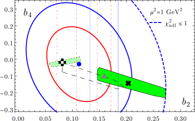
Figure 1: Results of the two-step fitting procedure described in the text. The following notations are used: BMS DA—black cross ✖ Bakulev et al. (2001); platykurtic DA—black/white cross ✜ Stefanis (2014); Stefanis and Pimikov (2016); DA shown as a grey triangle ▲ selected from the BMS set of DAs to be inside the $1\sigma$ error ellipse (innermost red line) while fulfilling the N³LO (vertical solid lines) lattice constraints on $b_{2}$ from lattice QCD Bali et al. (2019). Left: first step of this procedure in which we determine the admissible regions of the higher-twist parameters $\delta_{\text{tw-4}}^{2}$ and $\delta_{\text{tw-6}}^{2}$. The larger rectangle denotes the range of values with $\delta_{\text{tw-6}}^{2}=(1.84^{+0.84}_{-0.24})\,\times 10^{-4}\,\text{GeV}^{6}$, obtained in Cheng et al. (2020), while the smaller rectangle corresponds to the estimate $\delta_{\text{tw-6}}^{2}=(1.76\pm 0.13)\,\times 10^{-4}\,\text{GeV}^{6}$. This estimate and the red point $\delta_{\text{tw-6}}^{2}=(1.61\pm 0.26)\times 10^{-4}$ GeV⁶ were obtained in this work. Right: results of the fitting procedure for the twist-two conformal coefficients $b_{2},b_{4}$ with fixed higher-twist parameters. The two rectangles along the lower diagonal denote the range of $(b_{2},b_{4})$ determined within the BMS approach Bakulev et al. (2001) for two different values of $\lambda_{q}^{2}=0.4$ GeV² (larger shaded rectangle) and 0.45 GeV² (transparent rectangle), where the BMS DA Bakulev et al. (2001) is represented by ✖. The smaller shaded rectangle encloses the range of $(b_{2},b_{4})$ coefficients associated with DAs having a platykurtic profile Stefanis and Pimikov (2016), like the model ✜ proposed in Stefanis (2014). The dashed-dotted, dashed, and solid vertical lines show the lattice results for $b_{2}$ from Bali et al. (2019) for the NLO ($0.109(37)$), NNLO ($0.139(32)$), and N³LO ($0.159_{-0.027}^{+0.025}$), respectively.

According to the exposition above, the domain of small $Q^{2}$ values under single-tag conditions becomes now accessible to a trustworthy perturbative description within the FAPT/LCSR scheme using the TFF expression (26), which involves resummed radiative corrections. On the other hand, the higher-twist contributions can be safely included within FOPT, see Mikhailov et al. (2016); Stefanis (2020). This allows for the first time a detailed and reliable comparison with the recently released data with an unprecedented accuracy below $Q^{2}=1.5$ GeV² of the BESIII experiment Redmer (2018); Ablikim et al. (2020). Because of the competitive accuracy up to 3.1 GeV² of these data, it is possible to combine them with the measurements of previous single-tag experiments, notably, CELLO Behrend et al. (1991) and CLEO Gronberg et al. (1998) within the same range of momenta. This way, we can perform a simultaneous best-fit analysis of these data sets with the aim to determine the values of the involved nonperturbative parameters in the calculation of the TFF. These are the conformal coefficients $b_{2}$ and $b_{4}$ at twist-two in Eq. (2a), and the scale parameters for the twist-four, $\delta^{2}_{\text{tw4}}$, and the twist-six, $\delta^{2}_{\text{tw6}}$, terms, given in Appendix B. At the normalization scale $\mu^{2}_{0}=1$ GeV², the mentioned parameters assume values in the following ranges

$$\text{twist-two BMS DA domain~{}\cite[cite]{\@@bibref{Authors Phrase1YearPhrase2}{Bakulev:2001pa,Bakulev:2002uc,Bakulev:2004mc}{\@@citephrase{(}}{\@@citephrase{)}}}}: \Big{\{}b_{2}(\mu_{0}^{2})\!=\![0.146,0.272],\,\,b_{4}(\mu_{0}^{2})\!=\![-0.23,-0.049]\Big{\}}$$ (28a)

$$\text{twist-four~{}\cite[cite]{\@@bibref{Authors Phrase1YearPhrase2}{Bakulev:2002uc}{\@@citephrase{(}}{\@@citephrase{)}}}}: \delta_{\text{tw-4}}^{2}(\mu^{2}_{0})=0.19\pm 0.04~{}\text{GeV}^{2}$$ (28b)

$$\text{twist-six}\,: \delta_{\text{tw-6}}^{2}(\mu^{2}_{0})=\bigg{\{}\begin{array}[]{l}\langle\sqrt{\alpha_{s}}\bar{q}q\rangle^{2}=(1.76\pm 0.13)\,\times 10^{-4}\,\text{GeV}^{6}\text{(here)}\\ \langle\sqrt{\alpha_{s}}\bar{q}q\rangle^{2}=\left(~{}1.84^{+0.84}_{-0.24}~{}\right)\,\,\times 10^{-4}\,\text{GeV}^{6}\,\text{\cite[cite]{\@@bibref{Authors Phrase1YearPhrase2}{Cheng:2020vwr}{\@@citephrase{(}}{\@@citephrase{)}}}}\,.\end{array}$$ (28e)

Fitting procedure—step 1. We perform a data fit that proceeds in two steps: First, we use Eqs. (26), (27) to determine best-fit values of the higher-twist parameters $\delta_{\text{tw-4}}^{2},~{}\delta_{\text{tw-6}}^{2}$ keeping the twist-two nonperturbative coefficients $b_{2}$ and $b_{4}$ fixed, see left panel of Fig. 1. This gives rise to stretched out ellipses that degenerate into strips. These strips for different DA models taken from the BMS-like family, cf. (28a) overlap almost completely. Such strips with $\chi^{2}_{\text{ndf}}\leqslant 1$ are displayed in the figure. The uncertainties related to the higher-twist scales are shown graphically in terms of shaded rectangles with respect to the central values of the $\delta_{\text{tw-4}}^{2}$ and $\delta_{\text{tw-6}}^{2}$ scales in (28e). The fitting is done by employing particular DAs with $b_{2},b_{4}$ values at 1 GeV obtained within QCD sum rules with nonlocal condensates:

1. BMS model ($b_{2}=0.203$, $b_{4}=-0.143$) (✖)—the center of the BMS domain Bakulev et al. (2001),

2. platykurtic (pk) $(b_{2}=0.0812,b_{4}=-0.0191)$ (✜) Stefanis (2014); Stefanis and Pimikov (2016)—see Stefanis (2020) for further discussion,

3. $(b_{2}=0.159,b_{4}=-0.098)$ ▲—crossing point of the N³LO mean value from lattice Bali et al. (2019) with the long axis of the BMS domain, see the right panel of Fig. 1

These DAs can be used to fix the variations of the twist-two contributions and thus enable the determination of the best-fit centers of the confidence ellipses for the scale coefficients $\delta_{\text{tw-4}}^{2},~{}\delta_{\text{tw-6}}^{2}$. In fact, the main result of this fitting procedure is that all determined strips have a common long axis. This implies that these parameters are strongly correlated and are aligned with this regression line. On the other hand, this ascertained quasilinear dependence would entail an unpleasant overfitting of the best-fit positions of $\delta_{\text{tw-4}}^{2},~{}\delta_{\text{tw-6}}^{2}$ for the particular DAs. Therefore, we proceed differently. Using the mean value of $\delta_{\text{tw-4}}^{2}$ from Eq. (28b), this axis yields for the twist-six prefactor the value $\delta_{\text{tw-6}}^{2}=(1.61\pm 0.26)\times 10^{-4}$ GeV⁶, where the error margin can be determined by imposing the condition $\chi^{2}_{\text{ndf}}\leqslant 1$. This result bears no dependence on the choice of a particular model DA. This $\delta_{\text{tw-6}}^{2}$ value—the red dot at the bottom of the rectangles in the figure—is in good agreement with different independent estimates of $\delta_{\text{tw-6}}^{2}$ at its low limit. This is outlined in Eq. (28e) and is discussed in more detail in Appendix B. It corresponds to the dark violet rectangle in the left panel of Fig. 1.

Fitting procedure—step 2. We can now use the best-fit values of the twist-four and twist-six parameters ($\delta_{\text{tw-4}}^{2}=0.19$ GeV² and $\delta_{\text{tw-6}}^{2}=1.61\times 10^{-4}$ GeV⁶) to derive the confidence regions of the twist-two expansion parameters $b_{2}$ and $b_{4}$. The results of this step of the fitting procedure are displayed in the right panel of Fig. 1. The best-fit point with $\chi^{2}_{\text{ndf}}=0.38$ is marked by the thick blue dot ($b^{\text{b-f}}_{2}=0.112$, $b^{\text{b-f}}_{4}=-0.029$), whereas the $1\sigma$ error ellipse and the $2\sigma$ error ellipse are denoted by the innermost red solid line and the blue solid line, respectively. The outermost blue dashed ellipse corresponds to $\chi^{2}_{\text{ndf}}=1$. In close correspondence to the left panel, we also show the positions of the considered DA models at the normalization scale $\mu_{0}=1$ GeV. The other ingredients of Fig. 1 (right panel) are the following:

• Large shaded rectangle in green color—BMS domain with the coefficients $b_{2},b_{4}$ given above, for the average virtuality of vacuum quarks $\lambda_{q}^{2}=0.40$ GeV² Bakulev et al. (2001),

• Transparent rectangle bounded by a dashed line—domain of BMS DAs obtained for the larger virtuality $\lambda_{q}^{2}=0.45$ GeV².

• Small light-green rectangle—platykurtic range Stefanis and Pimikov (2016) for the pk DA ✜ Stefanis (2014).

• We also display for comparison, the most recent lattice constraints on $b_{2}$ from Bali et al. (2019) using vertical lines. These are obtained from left to right with NLO matching to $\overline{\rm MS}$ scheme (dashed-dotted red lines), NNLO matching (dashed red lines), and N³LO, i.e., three-loop matching (solid blue lines). This sequence of lines exhibits the progressive change of these constraints as the loop order increases and the width of the corresponding strip decreases. It is worth noting in this context that the various uncertainties of the lattice constraints have been added in quadrature which means that they are dominated by the largest systematic error originating from the nonperturbative renormalization using the regularization independent momentum subtraction (RI’/MOM) scheme Bali et al. (2019); Martinelli et al. (1995).

From this figure we can draw the following conclusions.

1. The different sources of data below $Q^{2}\leq 3.1$ GeV² give rise to a $2\sigma$ error ellipse (based on the NLLA) which has a significant overlap with a large part of the BMS domain and also the lattice constraints at the NNLO and N³LO level, restricting the values of $b_{2}$ to the range $[0.107,0.184]$.

2. A good portion of the BMS domain for $b_{2}^{\text{BMS}}<0.171$ lies within the $1\sigma$ confidence ellipse of the data and also inside the N³LO lattice strip. This compatibility provides support to the BMS nonperturbative scheme and its ingredients.

3. Imposing the most stringent combination of these constraints—$1\sigma$ ellipse and N³LO lattice range—one can determine a DA within the BMS domain defined by the crossing point of the N³LO lattice value $b_{2}=0.159$ (at $\mu^{2}_{0}=1$ GeV²) with the long axis of the BMS rectangle to obtain the value $b_{4}=-0.098$. This uniquely defined DA with the parameters ($b_{2}=0.159,b_{4}=-0.098$) provides a good compromise for the simultaneous fulfillment of three distinct types of constraints originating from different sources. It is denoted in Fig. 1 by ▲ and is used in the following section to obtain predictions for the TFF.

4. Note that an analogous crossing point of the NNLO middle point with the long BMS line would fulfill the same requirements but would be outside the BMS rectangle.

5. The platykurtic range lies entirely within the $1\sigma$ confidence ellipse and is close to the lattice NNLO strip.

V TFF predictions in the range $Q^{2}\leqslant 5.5$ GeV² vs data

In this section, we present our TFF predictions obtained within the FAPT/LCSR scheme developed in the previous sections. We have two main objectives: To compare with various data up to an intermediate momentum $Q^{2}=5.5$ GeV² and doing this to expose the improvements relative to the FOPT/LCSR results. Different approaches applicable to the calculation of the TFF in the low-$Q^{2}$ regime, are mentioned in Stefanis (2020). We include the full data sets of the BESIII Redmer (2018) and CELLO Behrend et al. (1991) Collaborations and also the measurements below 5.5 GeV² of the CLEO Gronberg et al. (1998), BaBar Aubert et al. (2009), and Belle Uehara et al. (2012) experiments. The BESIII data with their errors have been extracted from the graphics in Fig. 3 of Redmer (2018) using the tool PlotDigitizer Rohatgi (2020) and are tabulated in Table 1. This restricted data selection is justified because our primary goal is to show the utility of the summation technique in performing a LCSR calculation below/around 1 GeV². At high $Q^{2}$, one can rely upon the FOPT/LCSR method, see Stefanis (2020) for such predictions and a complete list of the other data. An alternative approach attempting to determine the higher moments of the twist-two pion DA more reliably, was recently proposed in Zhong et al. (2021). We note in similar context the Dyson-Schwinger-equations based approach recently reviewed in Roberts et al. (2021) which uses a basis of Gegenbauer polynomials whose degree is included in the optimization procedure to improve the convergence of the polynomial expansion.

The TFF calculation is performed at the NNLO${}_{\beta_{0}}$ for FOPT and in the NLLA for FAPT (see Eqs. (27)). Using the expansion in Eq. (2) and the partial TFF terms $F^{\gamma\pi}_{\text{LCSR/FAPT;n}}$ from Eqs. (26), (27), we obtain predictions for $Q^{2}F^{\gamma\pi}_{\text{FAPT}}(Q^{2})$ in terms of the conformal coefficients $\{1,b_{2},b_{4},\ldots\}$ that can be used for any pion DA (for a more detailed derivation at this level of accuracy, see Mikhailov et al. (2016); Stefanis (2020) and references cited therein). The results are shown graphically in Fig. 2.

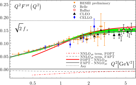
Figure 2: Theoretical predictions for the scaled $\gamma^{*}\gamma\pi^{0}$ transition form factor $Q^{2}F^{\gamma\pi}_{\text{FAPT}}(Q^{2})$ [GeV] using different DAs discussed in the text in comparison with various data up to $Q^{2}<5.5$ GeV² with labels as indicated in the figure. The grey and the red solid lines were obtained with the DA denoted by ▲ using the FAPT/LCSR and FOPT/LCSR scheme, respectively. The black dashed line represents the FAPT result obtained with the pk-DA Stefanis (2014), while the green strip shows the theoretical uncertainties of the BMS DAs calculated with QCD sum rules with nonlocal condensates Bakulev et al. (2001). The displayed FAPT/FOPT TFF results employ the best-fit nonperturbative higher-twist parameters $\delta_{\text{tw-4}}^{2}=0.19$ GeV² and $\delta_{\text{tw-6}}^{2}=1.61\times 10^{-4}$ GeV⁶.

$Q^{2}$ [GeV2]	0.351	0.45	0.551	0.652	0.751	0.851	0.951	1.075	1.226	1.374	1.526	1.701	1.901	2.101	2.3	2.5	2.7	2.95
$\Delta Q^{2}$	0.05	0.049	0.05	0.05	0.049	0.052	0.049	0.073	0.075	0.074	0.075	0.101	0.1	0.099	0.101	0.099	0.1	0.15
$Q^{2}F(Q^{2})$	0.057	0.068	0.073	0.081	0.087	0.091	0.099	0.107	0.116	0.113	0.113	0.121	0.117	0.14	0.131	0.123	0.164	0.135
$Q^{2}\Delta F(Q^{2})$	0.006	0.005	0.004	0.004	0.004	0.008	0.008	0.006	0.009	0.011	0.016	0.017	0.016	0.024	0.024	0.034	0.049	0.044

Table 1: Preliminary BESIII data on the scaled pion-photon TFF extracted from Fig. 3 in Redmer (2018).

With reference to Fig. 1, we display the TFF derived with the DAs from the BMS domain (large shaded rectangle) in the form of a green strip with a variable width quantifying the variation of these predictions entailed by the theoretical uncertainties of their key ingredients. These are resolved at the bottom of the figure in order to give quantitative estimates of their relevance (see the graphical explanations inside Fig. 2). Note that all displayed results are obtained by using in Eq. (26) the soft $V$-part given by Eqs. (27b), (27d) and including the vector resonances $\rho$ and $\omega$ in the form of a Breit-Wigner distribution, see Appendix D. This induces an additional factor that depends on the Borel parameter $M^{2}$, taken to vary in the interval (0.75–1.1) GeV² and depending on the momentum $Q^{2}$ as in Bakulev et al. (2011, 2012). The masses and widths of the vector resonances are $m_{\rho}=0.77$ GeV, $\Gamma_{\rho}=0.1502$ GeV, $m_{\omega}=0.7826$ GeV, $\Gamma_{\omega}=0.00844$ GeV. The other LCSR parameters have been fixed in previous investigations to the values Khodjamirian (1999); Bakulev and Mikhailov (2002) $f_{\pi}=0.132$ GeV, $s_{0}\approx 1.5~{}\text{GeV}^{2}$, $\delta_{\text{tw-4}}^{2}(\mu^{2}_{0})=0.95\,\lambda^{2}_{q}/2=0.19~{}\text{GeV}^{2}$ Bakulev et al. (2003) and are not varied here. The twist-six scale $\delta_{\text{tw-6}}^{2}(\mu^{2}_{0})=\langle\sqrt{\alpha_{s}}\bar{q}q\rangle^{2}(\mu^{2}_{0})=1.61\times 10^{-4}\text{GeV}^{6}$ was determined in Sec. IV by a fit to the experimental data under the condition $\delta_{\text{tw-4}}^{2}=0.19\,\text{GeV}^{2}$, (see the previous section) and is approximately equal to the lower bound of the estimates in (28b), (28e). Finally, the strong coupling $\alpha_{s}(\mu_{0}^{2})=0.48\pm 0.024$, as well as the evolution of the DAs, are both taken in the two-loop approximation, see Appendix A in Stefanis (2020).

The other displayed TFF predictions are the following. The FAPT/LCSR TFF for the DA denoted by the symbol ▲, is shown by the solid grey line, while the analogous result for the FOPT/LCSR TFF is represented by the solid red line. For both curves the same values of the twist-four and twist-six parameters are used. The displayed red curve serves only to demonstrate the tendency of the FOPT/LCSR result to underestimate the data. In fact, at 0.5 GeV² the calculated TFF is already outside the applicability domain of this scheme. In contrast, the FAPT/LCSR prediction, given by the light-grey line, reproduces the data for momenta below $Q^{2}=5.5$ GeV² and down to values as low as $0.3$ GeV² with an accuracy of $\chi^{2}_{\text{ndf}}=0.57$. It is remarkable that the TFF calculated with the platykurtic DA (✜) Stefanis (2014) (black dashed line) turns out to be close to this line with $\chi^{2}_{\text{ndf}}=0.77$. This agrees with the results obtained recently within FOPT/LCSR in Stefanis (2020). An important observation from the curves shown at the bottom of Fig. 2 is that above $Q^{2}>2$ GeV², the NNLO_β parts of both LCSR schemes (FOPT–dashed-dotted line and FAPT—dashed line) yield congruent results. Below $Q^{2}\lesssim 1$ GeV², the RG summation of the radiative corrections (dashed line at the bottom) in the FAPT/LCSR scheme avoids the overestimation of the NNLO correction in the FOPT/LCSR scheme (dashed red line at the bottom), clearly demonstrating its superiority.

VI Conclusions

In this work we developed and outlined a new theoretical scheme to calculate the pion-photon transition form factor with single-tag kinematics that involves RG summation of radiative corrections while avoiding Landau singularities of the running strong coupling. We showed that this scheme, termed FAPT/LCSR, is capable of providing trustworthy results well below the typical hadronic scale of 1 GeV, a regime not reliably accessible using FOPT/LCSR. This allows the comparison of theoretical predictions with the recently released preliminary data of the BESIII Collaboration Redmer (2018) which bear very small errors just in this momentum region.

To include the hadronic content of the quasireal photon, we used in the phenomenological part of the LCSR a Breit-Wigner distribution which provides a more realistic representation than a simple $\delta$-function ansatz. This admits the possibility of comparing more precisely the obtained TFF predictions with those in the state-of-the-art analysis within FOPT/LCSR in Stefanis (2020), which also employs the Breit-Wigner form. This way, the effect of including the QCD radiative corrections by means of RG summation has been properly determined. Doing so, we were able to substantially exceed our exploratory analysis in Ayala et al. (2018a, 2019) and promote our understanding of the TFF behavior at much lower momentum scales. In the following we collect and discuss further the key results of our analysis.

(i) We used the available experimental data in the low-momentum domain up to $Q^{2}\leq 3.1$ GeV² in order to determine best-fit values of the higher-twist parameters.

Especially the measurement of the BESIII experiment Redmer (2018) provided data with an unprecedented accuracy below $Q^{2}=1.5$ GeV². Using this data set in combination with previous data of the CELLO Behrend et al. (1991) and CLEO Gronberg et al. (1998) Collaborations, we obtained a reliable estimate for the twist-six contribution $\delta_{\text{tw-6}}^{2}=1.61\times 10^{-4}$ GeV⁶ using $\delta_{\text{tw-4}}^{2}=0.19$ GeV² from  Bakulev et al. (2003) and keeping the conformal coefficients $b_{2}$ and $b_{4}$ within the BMS domain.

(ii) In the second step, we used these parameters to extract the most trustworthy regimes of the conformal coefficients ($b_{2},b_{4}$) by applying additional constraints from the data and the most recent lattice calculations of $b_{2}$. To be precise, we determined the $1\sigma$ and $2\sigma$ error ellipses of the data and combined them with the lattice constraints of Bali et al. (2019) at the NNLO, and N³LO level. Combing these constraints in the most stringent way, we found that the crossing point of the middle value of the N³LO lattice range of $b_{2}$ with the long axis of the BMS domain Bakulev et al. (2001) of the ($b_{2},b_{4}$) values, defines a DA, marked by the symbol ▲, that agrees with the employed data at the $1\sigma$ level.

(iii) Employing this DA as nonperturbative input, we performed a twin-calculation of the TFF in FAPT/LCSR and in FOPT/LCSR in order to quantify the advantage of including the radiative corrections via RG summation. The corresponding TFF curves are shown in Fig. 2 in terms of a grey and a red curve, respectively. One appreciates that the FAPT result reproduces the data in a momentum range starting below $1$ GeV² and extending up to 5.5 GeV² at the level of an overall accuracy of $\chi^{2}_{\text{ndf}}=0.57$.

(iv) The FAPT/LCSR TFF result for the platykurtic pion DA Stefanis (2014), shown as a black dashed line in Fig. 2, follows closely the grey curve and the BMS strip (in green color) of predictions though this DA has a unimodal profile in contrast to the bimodal shapes of the BMS DAs. This can be traced to the values of their inverse moments that almost coincide. For the discussion of the properties of this DA, we refer to Stefanis (2020).

As a last remark, we mention that our exposed method may be useful in providing insight into the hadronic light-by-light contribution of the g-2 of the muon, see Masjuan (2012); Dorokhov et al. (2014) and Aoyama et al. (2020) for a recent review. Moreover, a pion DA very close to ▲ was used very recently in Leljak et al. (2021) (see Table 1) to calculate the $\bar{B}\rightarrow\pi$ form factors and determine $|V_{ub}|$ in agreement with inclusive estimates.

Appendix A QCD perturbative expansion beyond leading order

NLO. The coefficient function of the partonic subprocess $\mathcal{T}^{(1)}$ is

$$\frac{{\cal T}^{(1)}(x,y)}{C_{\rm F}} = \left[-3V^{b}+g\right]_{+}(x,y)-3\delta(x-y),$$ (29a)

$$g_{+}(x,y) = -2\left[\theta(y>x)\frac{\ln\left(1-x/y\right)}{y-x}\right.$$ (29b)

$$\hskip 19.91692pt\left.+\theta(y<x)\frac{\ln(1-\bar{x}/\bar{y})}{x-y}\right]_{+},~{}~{}~{}$$

while the elements of the one-loop evolution kernel $V_{0}$ are

$$\frac{V_{0}(x,y)}{C_{\rm F}} = V^{(0)}_{+}(x,y)=2\left[{\cal C}\theta(y>x)\frac{x}{y}\left(1+\frac{1}{y-x}\right)\right]_{+}$$ (30a)

$$\equiv 2\left[V^{a}(x,y)+V^{b}(x,y)\right]_{+}\,,$$

$$V^{a}(x,y) = {\cal C}\theta(y>x)\frac{x}{y},$$

$$V^{b}(x,y) = {\cal C}\theta(y>x)\frac{x}{y}\left(\frac{1}{y-x}\right)\,,$$ (30b)

where the symbol $\mathcal{C}$ means ${\cal C}=\hbox{{1}\kern-2.5pt\hbox{l}}+\left\{x\to\bar{x},y\to\bar{y}\right\}$. The key term of the convolution ${\cal T}^{(1)}(x,y)\otimes\psi_{n}(y)$ that enters the harmonic expansion can be significantly simplified to get

$$\frac{1}{C_{\rm F}}{\cal T}^{(1)}(x,y)\underset{y}{\otimes}\psi_{0}(y) = \left[-3+\frac{\pi^{2}}{3}-\ln^{2}\left(\frac{\bar{x}}{x}\right)\right]\psi_{0}(x)-2~{}\psi_{0}(x),$$ (31)

$$\frac{1}{C_{\rm F}}{\cal T}^{(1)}(x,y)\underset{y}{\otimes}\psi_{n}(y) = \left[-3\left(1+v^{b}(n)\right)+\frac{\pi^{2}}{3}-\ln^{2}\left(\frac{\bar{x}}{x}\right)\right]\psi_{n}(x)-2\sum^{n}_{l=0,2,\ldots}\!\!\!G_{nl}\psi_{l}(x)\,,$$ (32)

$$v^{b}(n) = 2\left(\psi(2)-\psi(2+n)\right);~{}v(n)=1/\left[(n+1)(n+2)\right]-1/2+2\left(\psi(2)-\psi(2+n)\right)\,,$$ (33)

see Appendix A in Mikhailov and Stefanis (2009). The quantities $v^{b}(n)$ and $v(n)=-\frac{1}{2C_{\rm F}}\frac{1}{2}\gamma_{0}(n)$ are the eigenvalues of the elements $V^{b}_{+}$ and $V^{a}_{+}+V^{b}_{+}$ of the one-loop kernel in Eq. (30a), respectively. $G_{nl}$ denotes the elements of a calculable triangular matrix (omitted here)—see for details Mikhailov and Stefanis (2009) and corrections in Agaev et al. (2011).

The explicit expressions for the first coefficients of the expansion of the QCD $\beta$ function are

$$\beta_{0}=\frac{11}{3}\,C_{\text{A}}-\frac{4}{3}\,T_{r}N_{f}\,,\qquad\beta_{1}=\frac{34}{3}\,C_{\text{A}}^{2}-\left(4C_{\text{F}}+\frac{20}{3}\,C_{\text{A}}\right)T_{r}N_{f}\,.$$ (34)

NNLO. The $\beta_{0}$ part of the coefficient function ${\cal T}^{(2)}$, the $\beta_{0}{\cal T}^{(2)}_{\beta}$ term, reads

$${\cal T}^{(2)}_{\beta}(x,y) = C_{\rm F}\Bigg{[}\frac{29}{12}2V^{a}+2\dot{V}^{a}-\frac{209}{36}V^{(0)}-\frac{7}{3}\dot{V}^{(0)}-\frac{1}{4}\ddot{V}^{(0)}+\frac{19}{6}g+\dot{g}\Bigg{]}_{+}\!\!(x,y)-6C_{\rm F}\delta(x-y)\,.$$ (35)

This expression was originally derived in Melić et al. (2003), but its elements are presented here using a different notation following Mikhailov and Stefanis (2009), where also the omitted explicit expressions for the elements $\dot{V}^{a},\dot{V}^{(0)},\ddot{V}^{(0)}$ and $\dot{g}$ can be found.

Appendix B Higher-twist contributions

The explicit expressions for the twist-four and twist-six Agaev et al. (2011) contributions are given by

$$\bar{\rho}_{\text{tw-4}}(Q^{2},x)=\frac{\delta_{\text{tw-4}}^{2}(Q^{2})}{Q^{2}}x\frac{d}{dx}\varphi^{(4)}(x);$$ (36)

$$\varphi^{(4)}(x)=\frac{80}{3}x^{2}(1-x)^{2}\,,$$

$$\delta_{\text{tw-4}}^{2}(Q^{2})=\left[\frac{a_{s}(Q^{2})}{a_{s}(\mu^{2}_{0})}\right]^{\frac{\gamma_{T4}}{\beta_{0}}}\delta_{\text{tw-4}}^{2}(\mu^{2}_{0})\,,$$ (37)

$$\delta_{\text{tw-4}}^{2}(\mu^{2}_{0})=0.95\,\lambda^{2}_{q}/2=0.19~{}\text{GeV}^{2}~{}\text{\cite[cite]{\@@bibref{Authors Phrase1YearPhrase2}{Bakulev:2002uc}{\@@citephrase{(}}{\@@citephrase{)}}}}\,,\gamma_{T4}=32/9\,,$$

$$\bar{\rho}_{\text{tw-6}}(Q^{2}\!,x)=8\pi\frac{C_{F}}{N_{c}}\frac{\alpha_{s}\langle\bar{q}q\rangle^{2}}{f_{\pi}^{2}}\frac{x}{Q^{4}}\left[\!-\!\left(\frac{1}{1-x}\right)_{+}\right.$$

$$\hskip 65.44133pt\left.\!+\!\left(2\delta(\bar{x})-4x\right)\!+\!x\left(3+2\ln(x\bar{x})\right)\phantom{\left(\frac{1}{x}\right)_{+}}\right]\,~{}~{}~{}~{}~{}$$ (38)

at $\mu^{2}_{0}=1$ GeV².

The NLO evolution of the quark condensate $$\langle\bar{q}q\rangle(\mu^{2})$$ reads

$$\langle\bar{q}q\rangle(\mu^{2}) = \langle\bar{q}q\rangle(4\,\text{GeV}^{2})\left[\frac{\bar{a}_{s}^{(2)}(4\,\text{GeV}^{2})}{\bar{a}^{(2)}_{s}(\mu^{2})}\right]^{\nu}\!$$ (39a)

$$\hskip 22.76219pt\times\left[\frac{1+c_{1}\bar{a}_{s}^{(2)}(4\,\text{GeV}^{2})}{1+c_{1}\bar{a}^{(2)}_{s}(\mu^{2})}\right]^{\omega}~{}~{}$$

for $$N_{f}=3 \Lambda^{(3)}_{\text{MS}}=392$$, MeV with a two-loop running, where

$$\nu=\gamma_{0}/\beta_{0}\,,~{}\gamma_{0}=4\,,~{}\beta_{0}=11-\frac{2}{3}N_{f}\,,$$ (39b)

$$\beta_{1}=102-\frac{38}{3}N_{f}\,,~{}\omega=[\gamma_{1}\beta_{0}-\gamma_{0}\beta_{1}]/[\beta_{0}\beta_{1}]\,,~{}~{}~{}~{}~{}~{}$$ (39c)

$$\gamma_{1}=\frac{202}{3}-\frac{20}{9}N_{f}\,,~{}c_{1}=\beta_{1}/\beta_{0}\,.$$ (39d)

The quark-condensate density is obtained from the Gell-Mann-Oakes-Renner relation

$$\langle\bar{q}q\rangle(\mu^{2}) = -\frac{f_{\pi}^{2}m^{2}_{\pi}}{2(m_{u}+m_{d})(\mu^{2})}\,.$$ (40)

Taking into account the estimate $(m_{u}+m_{d})(\mu^{2}_{L}=4\text{GeV}^{2})=7.28(82)~{}\text{MeV}$ from lattice computations Tanabashi et al. (2018) and performing a two-loop running according to (39a), we obtain for a “quasi” (one-loop) RG invariant quantity the new estimate

$$\langle\sqrt{\alpha_{s}}\bar{q}q\rangle^{2}(\mu^{2}_{0}) = (1.76\pm 0.13)\,\times 10^{-4}\,\text{GeV}^{6}\,,~{}~{}~{}~{}$$ (41a)

$$\alpha_{s}(\mu^{2}_{0}) = 0.48\pm 0.024\,,$$

by employing a NLO approximation. A result for this quantity close to that was found in Cheng et al. (2020) within a similar approach using the RunDec code, see Fig. 1 (left panel):

$$\langle\sqrt{\alpha_{s}}\bar{q}q\rangle^{2}(\mu^{2}_{0}) = (1.84^{+0.84}_{-0.24})\,\times 10^{-4}\,\text{GeV}^{6}\,,~{}~{}~{}~{}$$ (41b)

$$\alpha_{s}(\mu^{2}_{0}) = 0.486\pm 0.024\,.$$

Our best-fit estimate $\delta_{\text{tw-6}}^{2}=\langle\sqrt{\alpha_{s}}\bar{q}q\rangle^{2}(\mu^{2}_{0})=(1.61\pm 0.26)\times 10^{-4}$ GeV⁶ overlaps within errors with both values given above.

Appendix C ERBL summation at NNLO

The conformal symmetry of the ERBL equation at the two-loop level of evolution is broken. This entails within the basis of Gegenbauer harmonics the appearance of a nondiagonal part along with the dominating diagonal one Mikhailov and Radyushkin (1985, 1986). We consider here the most significant diagonal part at the two-loop level of the evolution exponential in Eq. (3), notably,

$$\exp\left[-\int\limits_{a_{s}(\mu^{2})}^{\bar{a}_{s}(y)}\!\!\frac{V(\alpha;x,z)}{\beta(\alpha)}d\alpha\right]\underset{z}{\otimes}\psi_{n}(z)$$

$$\stackrel{{\scriptstyle 2\,\text{loop}}}{{\longrightarrow}} \exp\left[\int\limits_{a_{s}(\mu^{2})}^{\bar{a}_{s}(y)}\frac{\gamma_{n}(a)}{\beta(a)}da\right]\psi_{n}(x)=$$ (42)

$$\left[\frac{\bar{a}_{s}(y)}{a_{s}(\mu^{2})}\right]^{\nu_{n}}\left[\frac{1+c_{1}\bar{a}_{s}(y)}{1+c_{1}a_{s}(\mu^{2})}\right]^{\omega_{n}}\psi_{n}(x)\,,$$

where $a_{s}$ has a two-loop running and $c_{1}=\beta_{1}/\beta_{0}$, with $\beta_{i}$ being the expansion coefficients of the QCD $\beta$-function. The evolution exponent of the coupling is defined by $\displaystyle\nu_{n}=\gamma_{0}(n)/2\beta_{0}$, $\omega_{n}=[\gamma_{1}(n)\beta_{0}-\gamma_{0}(n)\beta_{1}]/[2\beta_{0}\beta_{1}]$. The corresponding diagonal part of the partial form factors $F_{n}^{\text{(tw=2)}}$ (in the $\{\psi_{n}\}$ basis) has the form

$$\!\!\!\!F_{n}^{\text{(tw=2)}}(Q^{2},q^{2})=N_{\text{T}}T_{0}(y)\underset{y}{\otimes}\!\left[\hbox{{1}\kern-2.5pt\hbox{l}}+\bar{a}_{s}(y)\mathcal{T}^{(1)}(y,x)+\bar{a}_{s}^{2}(y)\mathcal{T}^{(2)}(y,x)\right]\left(\frac{\bar{a}_{s}(y)}{a_{s}(\mu^{2})}\right)^{\nu_{n}}\left[\frac{1+c_{1}\bar{a}_{s}(y)}{1+c_{1}a_{s}(\mu^{2})}\right]^{\omega_{n}}\underset{x}{\otimes}\psi_{n}(x)\,.$$ (43)

Every harmonic $\psi_{n}$ generates under the two-loop evolution the contribution of off-diagonal higher harmonics Mikhailov and Radyushkin (1986), but these are small compared to the diagonal ones. Therefore, they are not considered here. Moreover, we use the following approximation to (43)

$$\!\!\!\!F_{n}^{\text{(tw=2)}}(Q^{2},q^{2}) \thickapprox \frac{N_{\text{T}}}{\underline{\left[a_{s}(\mu^{2})\right]^{\nu_{n}}}\left[1+c_{1}a_{s}(\mu^{2})\right]^{\omega_{n}}}T_{0}(y)\underset{y}{\otimes}\!\bigg{\{}\underline{\left[\bar{a}_{s}(y)\right]^{\nu_{n}}+\left[\bar{a}_{s}(y)\right]^{1+\nu_{n}}\mathcal{T}^{(1)}(y,x)}$$ (44)

$$+~{}\omega_{n}c_{1}\left[\left[\bar{a}_{s}(y)\right]^{1+\nu_{n}}+\left[\bar{a}_{s}(y)\right]^{2+\nu_{n}}\frac{(\omega_{n}-1)}{2}c_{1}+\left[\bar{a}_{s}(y)\right]^{2+\nu_{n}}\mathcal{T}^{(1)}(y,x)\right]$$

$$+\left[\bar{a}_{s}(y)\right]^{2+\nu_{n}}\mathcal{T}^{(2)}(y,x)\bigg{\}}\underset{x}{\otimes}\psi_{n}(x)\,,$$

where the last factor $\left[1+c_{1}\bar{a}_{s}(y)\right]^{\omega_{n}}$ in (43) has been expanded. The additional new terms are presented in the second and the third line of Eq. (44), while the terms with a “NLO structure”, cf. Eq. (4), in the first line are underlined.

Appendix D Pion TFF in LCSR with a Breit-Wigner resonance model

We present the original expression Ayala et al. (2018a) as the sum of a hard term $H$ and a vector-resonance term $V$

$$F^{\gamma\pi}_{\text{LCSR};n}\!\left(Q^{2}\right)\!=\!\frac{N_{\text{T}}}{Q^{2}}\!\left[H_{n}(Q^{2})\!+\!\frac{Q^{2}}{m^{2}_{\rho}}k(M^{2})V_{n}(Q^{2},M^{2})\right],\!\!\!\!$$

(45)

where the coefficient $k$ has been introduced to modify the original expression Ayala et al. (2018a) by modeling the rho-meson resonance contribution in terms of a BW distribution instead of a delta-function ansatz used in Ayala et al. (2018a). For the BW case, the coefficient $k(M^{2})$ takes the form

$$k(M^{2})\!=\!\frac{\int\limits_{4m_{\pi}^{2}}^{s_{0}}\!ds\,\left(\Delta_{\rho}(s)+\Delta_{\omega}(s)\right)m^{2}_{\rho}/s}{\!\!\int\limits_{4m_{\pi}^{2}}^{s_{0}}\!\!ds\left(\Delta_{\rho}(s)+\Delta_{\omega}(s)\right)\exp\left(\frac{m^{2}_{\rho}}{M^{2}}-\frac{s}{M^{2}}\right)}\,,$$ (46)

where the BW spectral densities are described by means of the mass $m_{V}$ and the width $\Gamma_{V}$ of the included resonances of the rho and omega mesons ($V=\rho\,,\omega$), i.e.,

$$\Delta_{V}(s)\equiv\frac{1}{\pi}\frac{m_{V}\Gamma_{V}}{\left(m_{V}^{2}-s\right)^{2}+m_{V}^{2}\Gamma_{V}^{2}}\ .$$ (47)

Replacing the BW model by a delta-function form $\Delta_{V}(s)\to\delta(s-m^{2}_{V})$, one gets for the coefficient $k(M^{2})$

$$k(M^{2})\to k_{\delta}(M^{2})=1\,.$$ (48)

This reduces Eq. (45) to the form given in Ayala et al. (2018a).

References

• Balitsky et al. (1989) I. I. Balitsky, V. M. Braun, and A. V. Kolesnichenko, Nucl. Phys. B312, 509 (1989).
• Khodjamirian (1999) A. Khodjamirian, Eur. Phys. J. C6, 477 (1999), eprint hep-ph/9712451.
• Ayala et al. (2018a) C. Ayala, S. V. Mikhailov, and N. G. Stefanis, Phys. Rev. D 98, 096017 (2018a), [Erratum: Phys. Rev. D 101, 059901 (2020)], eprint 1806.07790.
• Ayala et al. (2019) C. Ayala, S. V. Mikhailov, A. V. Pimikov, and N. G. Stefanis, EPJ Web Conf. 222, 03017 (2019), eprint 1911.02845.
• Efremov and Radyushkin (1980) A. V. Efremov and A. V. Radyushkin, Theor. Math. Phys. 42, 97 (1980).
• Lepage and Brodsky (1980) G. P. Lepage and S. J. Brodsky, Phys. Rev. D22, 2157 (1980).
• Bakulev et al. (2005) A. P. Bakulev, S. V. Mikhailov, and N. G. Stefanis, Phys. Rev. D72, 074014 (2005), [Erratum: Phys. Rev. D72, 119908 (2005)], eprint hep-ph/0506311.
• Bakulev et al. (2007) A. P. Bakulev, S. V. Mikhailov, and N. G. Stefanis, Phys. Rev. D75, 056005 (2007), [Erratum: Phys. Rev. D77, 079901 (2008)], eprint hep-ph/0607040.
• Shirkov and Solovtsov (1997) D. V. Shirkov and I. L. Solovtsov, Phys. Rev. Lett. 79, 1209 (1997), eprint hep-ph/9704333.
• Shirkov and Solovtsov (2007) D. V. Shirkov and I. L. Solovtsov, Theor. Math. Phys. 150, 132 (2007), eprint hep-ph/0611229.
• Bakulev (2009) A. P. Bakulev, Phys. Part. Nucl. 40, 715 (2009), eprint 0805.0829.
• Stefanis (2013) N. G. Stefanis, Phys. Part. Nucl. 44, 494 (2013), eprint 0902.4805.
• Karanikas and Stefanis (2001) A. I. Karanikas and N. G. Stefanis, Phys. Lett. B504, 225 (2001), [Erratum: Phys. Lett. B636, no.6, 330 (2006)], eprint hep-ph/0101031.
• Redmer (2018) C. F. Redmer (BESIII), in 13th Conference on the Intersections of Particle and Nuclear Physics (CIPANP 2018) Palm Springs, California, USA, May 29-June 3, 2018 (2018), eprint 1810.00654.
• Stefanis (2019) N. G. Stefanis, Pion-photon transition form factor in QCD. Theoretical predictions and topology-based data analysis (2019), eprint 1904.02631.
• Stefanis (2020) N. G. Stefanis, Phys. Rev. D 102, 034022 (2020), eprint 2006.10576.
• Bali et al. (2019) G. S. Bali, V. M. Braun, S. Bürger, M. Göckeler, M. Gruber, F. Hutzler, P. Korcyl, A. Schäfer, A. Sternbeck, and P. Wein, JHEP 08, 065 (2019), [Addendum: JHEP 11, 037 (2020)], eprint 1903.08038.
• Bakulev et al. (2001) A. P. Bakulev, S. V. Mikhailov, and N. G. Stefanis, Phys. Lett. B508, 279 (2001), [Erratum: Phys. Lett. B590, 309 (2004)], eprint hep-ph/0103119.
• Rohatgi (2020) A. Rohatgi, Webplotdigitizer: Version 4.4 (2020), URL https://automeris.io/WebPlotDigitizer.
• Mikhailov and Stefanis (2009) S. V. Mikhailov and N. G. Stefanis, Nucl. Phys. B821, 291 (2009), eprint 0905.4004.
• Agaev et al. (2011) S. S. Agaev, V. M. Braun, N. Offen, and F. A. Porkert, Phys. Rev. D83, 054020 (2011), eprint 1012.4671.
• Mikhailov et al. (2016) S. V. Mikhailov, A. V. Pimikov, and N. G. Stefanis, Phys. Rev. D93, 114018 (2016), eprint 1604.06391.
• Ayala et al. (2017) C. Ayala, G. Cvetič, and R. Kögerler, J. Phys. G44, 075001 (2017), eprint 1608.08240.
• Ayala et al. (2018b) C. Ayala, G. Cvetič, R. Kögerler, and I. Kondrashuk, J. Phys. G45, 035001 (2018b), eprint 1703.01321.
• Melić et al. (2003) B. Melić, D. Müller, and K. Passek-Kumerički, Phys. Rev. D68, 014013 (2003), eprint hep-ph/0212346.
• Stefanis (2014) N. G. Stefanis, Phys. Lett. B738, 483 (2014), eprint 1405.0959.
• Stefanis and Pimikov (2016) N. G. Stefanis and A. V. Pimikov, Nucl. Phys. A945, 248 (2016), eprint 1506.01302.
• Cheng et al. (2020) S. Cheng, A. Khodjamirian, and A. V. Rusov, Phys. Rev. D 102, 074022 (2020), eprint 2007.05550.
• Ablikim et al. (2020) M. Ablikim et al., Chin. Phys. C 44, 040001 (2020), eprint 1912.05983.
• Behrend et al. (1991) H. J. Behrend et al. (CELLO), Z. Phys. C49, 401 (1991).
• Gronberg et al. (1998) J. Gronberg et al. (CLEO), Phys. Rev. D57, 33 (1998), eprint hep-ex/9707031.
• Bakulev et al. (2003) A. P. Bakulev, S. V. Mikhailov, and N. G. Stefanis, Phys. Rev. D67, 074012 (2003), eprint hep-ph/0212250.
• Bakulev et al. (2004) A. P. Bakulev, S. V. Mikhailov, and N. G. Stefanis, Annalen Phys. 13, 629 (2004), eprint hep-ph/0410138.
• Martinelli et al. (1995) G. Martinelli, C. Pittori, C. T. Sachrajda, M. Testa, and A. Vladikas, Nuclear Physics B 445, 81 (1995), ISSN 0550-3213, URL http://dx.doi.org/10.1016/0550-3213(95)00126-D.
• Aubert et al. (2009) B. Aubert et al. (BaBar), Phys. Rev. D80, 052002 (2009), eprint 0905.4778.
• Uehara et al. (2012) S. Uehara et al. (Belle), Phys. Rev. D86, 092007 (2012), eprint 1205.3249.
• Zhong et al. (2021) T. Zhong, Z.-H. Zhu, H.-B. Fu, X.-G. Wu, and T. Huang, An improved light-cone harmonic oscillator model for the pionic leading-twist distribution amplitude (2021), eprint 2102.03989.
• Roberts et al. (2021) C. D. Roberts, D. G. Richards, T. Horn, and L. Chang (2021), eprint 2102.01765.
• Bakulev et al. (2011) A. P. Bakulev, S. V. Mikhailov, A. V. Pimikov, and N. G. Stefanis, Phys. Rev. D84, 034014 (2011), eprint 1105.2753.
• Bakulev et al. (2012) A. P. Bakulev, S. V. Mikhailov, A. V. Pimikov, and N. G. Stefanis, Phys. Rev. D86, 031501(R) (2012), eprint 1205.3770.
• Bakulev and Mikhailov (2002) A. P. Bakulev and S. V. Mikhailov, Phys. Rev. D65, 114511 (2002), eprint hep-ph/0203046.
• Masjuan (2012) P. Masjuan, Phys. Rev. D86, 094021 (2012), eprint 1206.2549.
• Dorokhov et al. (2014) A. E. Dorokhov, A. E. Radzhabov, and A. S. Zhevlakov, JETP Lett. 100, 133 (2014), eprint 1406.1019.
• Aoyama et al. (2020) T. Aoyama et al., Phys. Rept. 887, 1 (2020), eprint 2006.04822.
• Leljak et al. (2021) D. Leljak, D. van Dyk, and B. Melić, The $\bar{B}\to\pi$ form factors from QCD and their impact on $|v_{ub}|$ (2021), eprint 2102.07233.
• Tanabashi et al. (2018) M. Tanabashi et al. (Particle Data Group), Phys. Rev. D 98, 030001 (2018).
• Mikhailov and Radyushkin (1985) S. V. Mikhailov and A. V. Radyushkin, Nucl. Phys. B254, 89 (1985).
• Mikhailov and Radyushkin (1986) S. V. Mikhailov and A. V. Radyushkin, Nucl. Phys. B273, 297 (1986).