Cosmology with LIGO/Virgo dark sirens: Hubble parameter and modified gravitational wave propagation

Abstract

We present a detailed study of the methodology for correlating ‘dark sirens’ (compact binaries coalescences without electromagnetic counterpart) with galaxy catalogs. We propose several improvements on the current state of the art, and we apply them to the GWTC-2 catalog of LIGO/Virgo gravitational wave (GW) detections, and the GLADE galaxy catalog, performing a detailed study of several sources of systematic errors that, with the expected increase in statistics, will eventually become the dominant limitation. We provide a measurement of $H_{0}$ from dark sirens alone, finding as the best result $H_{0}={67.3^{+27.6}_{-17.9}}\,\,{\rm km}\,{\rm s}^{-1}\,{\rm Mpc}^{-1}$ ($68\%$ c.l.) which is, currently, the most stringent constraint obtained using only dark sirens. Combining dark sirens with the counterpart for GW170817 we find $H_{0}={72.2^{+13.9}_{-7.5}}\,{\rm km}\,{\rm s}^{-1}\,{\rm Mpc}^{-1}$.

We also study modified GW propagation, which is a smoking gun of dark energy and modifications of gravity at cosmological scales, and we show that current observations of dark sirens already start to provide interesting limits. From dark sirens alone, our best result for the parameter $\Xi_{0}$ that measures deviations from GR (with $\Xi_{0}=1$ in GR) is $\Xi_{0}={2.1^{+3.2}_{-1.2}}$. We finally discuss limits on modified GW propagation under the tentative identification of the flare ZTF19abanrhr as the electromagnetic counterpart of the binary black hole coalescence GW190521, in which case our most stringent result is $\Xi_{0}={1.8^{+0.9}_{-0.6}}$.

We release the publicly available code $\tt{DarkSirensStat}$, which is available under open source license at https://github.com/CosmoStatGW/DarkSirensStat.

1 Introduction

In the last few years, gravitational wave (GW) astronomy and cosmology have become a reality. The detection of the first binary black hole (BBH) coalescence, GW150914 [1], was a historic moment; another milestone was the observation of the first binary neutron star (BNS) coalescence, GW170817, and of its electromagnetic counterpart [2, 3, 4, 5]. Since then, many additional detections have taken place, to the extent that, during the recent O3 LIGO/Virgo run, BBH coalescences have been detected at a rate of about $1.5$ per week. The recent release of the results from the first part of the O3 run (O3a) reports 39 candidate detections (of which, statistically, $\sim 3$ can be false alarms), including BBHs up to redshift $z\sim 0.8$ [6].

For applications to cosmology, the crucial feature of compact binary coalescences is that, from their GW signal, one can reconstruct the luminosity distance to the source [7], and for this reason they are referred to as ‘standard sirens’. Much work has been devoted to investigating the cosmological information that could be obtained from such measurements, either when the redshift of the source is provided by the observation of an electromagnetic counterpart, or using statistical methods, see e.g. [8, 9, 10, 11, 12, 13, 14, 15, 16, 17].

In a flat $\Lambda$CDM model, the expression for the luminosity distance as a function of redshift is given by

$$d_{L}(z)=\frac{c}{H_{0}}\,(1+z)\,\int_{0}^{z}\,\frac{d\tilde{z}}{\sqrt{\Omega_{M}(1+\tilde{z})^{3}+\Omega_{R}(1+\tilde{z})^{4}+\Omega_{\Lambda}}}\,,$$ (1.1)

where $\Omega_{M}$ and $\Omega_{R}$ are the present matter and radiation density fractions, respectively, and $\Omega_{\Lambda}$ is the energy density fraction associated to the cosmological constant, with $\Omega_{M}+\Omega_{R}+\Omega_{\Lambda}=1$ in the flat case. For completeness we have included the contribution from radiation; however, it is completely negligible at the redshifts relevant for standard sirens (we also neglect curvature, which can be trivially included). In the limit $z\ll 1$ we recover the Hubble law $d_{L}(z)\simeq(c/H_{0})z$, so from a measurement at such redshifts we can extract $H_{0}$.

The first measurement of $H_{0}$ from a standard siren has been possible thanks to the first observed BNS coalescence, GW170817. Using the information on the redshift coming from its electromagnetic counterpart gives $H_{0}=74^{+16}_{-8}\,{\rm km}\,{\rm s}^{-1}\,{\rm Mpc}^{-1}$ (median and symmetric $68.3\%$ credible interval), or $H_{0}=70^{+12}_{-8}\,\,{\rm km}\,{\rm s}^{-1}\,{\rm Mpc}^{-1}$ (maximum a posteriori $68.3\%$ interval) [18]. This was the first proof-of-principle that $H_{0}$ can be extracted from standard sirens. However, the error from this single detection is still too large to discriminate between the value of $H_{0}$ obtained from late-Universe probes [19, 20], and that inferred from early-Universe probes assuming $\Lambda$CDM [21, 22], which are currently in disagreement at $5.3\sigma$ level. One can estimate that ${\cal O}(50-100)$ standard sirens with counterpart are needed to reach the accuracy required to arbitrate this discrepancy [15, 16].

In the absence of a counterpart one can resort to statistical methods, in particular correlating the GW signal with galaxy catalogs, as already proposed in the pioneering work [7], and reformulated in a modern Bayesian framework in a number of more recent papers [13, 15, 16, 17] (see also [23, 24, 25, 26, 27, 28, 29] for recent related approaches exploiting galaxy clustering, and [30] for possible improvements from the detection of higher harmonics). In this context, compact binary coalescences without electromagnetic counterpart are often called ‘dark sirens’. The first application of the statistical method to actual data has been performed in [31], where a measurement of $H_{0}$ has been obtained from GW170817 without making use of the known electromagnetic counterpart, leading to a value $H_{0}=77^{+37}_{-18}\,\,{\rm km}\,{\rm s}^{-1}\,{\rm Mpc}^{-1}$. While the error is obviously larger than that obtained by making use of the counterpart, still this provides a proof-of-principle of the statistical method. A measurement of $H_{0}$ from a BBH dark siren was presented in [32], correlating the event GW170814 with the galaxy catalog from the Dark Energy Survey (DES), obtaining $H_{0}=75^{+40}_{-32}\,\,{\rm km}\,{\rm s}^{-1}\,{\rm Mpc}^{-1}$ (for a uniform prior in the range range $[20,140]\,\,{\rm km}\,{\rm s}^{-1}\,{\rm Mpc}^{-1}$). In [33] a similar analysis has been performed for the dark siren GW190814, which resulted from the coalescence of a $23M_{\odot}$ BH with a compact object with mass $2.6M_{\odot}$, leading to $H_{0}=66^{+55}_{-18}\,\,{\rm km}\,{\rm s}^{-1}\,{\rm Mpc}^{-1}$ when using the dark siren GW190814 only. In [34] the LIGO/Virgo collaboration (LVC) has obtained the value $H_{0}={69^{+16}_{-8}}\,\,{\rm km}\,{\rm s}^{-1}\,{\rm Mpc}^{-1}$ by combining the detections from the O1 and O2 runs, using GW170817 as a standard siren with counterpart, and the other events as dark sirens (with most of the improvement, with respect to using only GW170817, coming from GW170814, a well localized event that falls in the region of the sky covered by the DES catalog, which has a high level of completeness). While a significantly larger number of dark sirens will be needed in order to eventually obtain stringent constraints on $H_{0}$, these works provide the first concrete applications of the statistical method to the determination of $H_{0}$.

In the present paper we further develop the formalism of the statistical treatment of ‘dark sirens’, proposing improvements of various technical aspects. In particular, we include a direction-dependent notion of completeness of a galaxy catalog, we propose a novel method for dealing with incomplete catalogs, and we discuss in detail different approximations involved in the computation of the selection bias, including in its computation both the correct prior given by the galaxy catalog and additional selection effects related to the choice of the relevant GW events. We show that these improvements outperform state of the art methods. We will also extend our analysis to the determination of the parameters that characterize modified GW propagation, that, as we will discuss below, is the potentially most promising signal of deviations from General Relativity (GR) that can be accessed by standard sirens. We will finally apply the formalism to the most recent public data, including the O3a LIGO/Virgo run, both for the measurement of $H_{0}$ in the framework of $\Lambda$CDM, and for limits on modified GW propagation in the framework of modified gravity.

The paper is organized as follows. In sect. 2 we will review (following mostly [35, 36]) how, in modified gravity, the quantity measured from the coalescence of standard sirens is not the standard luminosity distance but a different quantity, that we called the ‘GW luminosity distance’, and which is sensitive to modifications of the propagation equation of tensor modes over a cosmological background. Such modifications are always present in modified gravity theories and can give a potentially very large effect (reaching even $80\%$ at large redshifts, in some models that are phenomenologically viable). This makes modified GW propagation a potentially very interesting observable for GW detectors, already in their current second-generation (2G) stage. In sect. 3 we present the formalism that we will use for dark sirens, based on a hierarchical Bayesian framework, and we will discuss in great detail a number of technical aspects (in particular related to methods for dealing with catalog incompleteness and with crucial normalization factors), proposing various improvements. We will then discuss our results in sect. 4, applying this formalism to the most recent LIGO/Virgo data. Sect. 5 contains our conclusions. Some further technical material is collected in various appendices.

2 GW luminosity distance in modified gravity

2.1 Modified GW propagation

Even if, to date, the study of the LIGO/Virgo standard sirens has been mostly focused on obtaining from them a measurement of $H_{0}$, eventually the most interesting result would be the observation of effects that can be directly traced to dark energy (DE) and modifications of GR on cosmological scales. As usual, on cosmological scales it is convenient to perform a separation between the homogeneous Friedmann-Robertson-Walker (FRW) background, and scalar, vector and tensor perturbations over it. In a generic modified gravity theory, both the background evolution and the perturbations differ from that in $\Lambda$CDM. At the background level, the effect of deviations from $\Lambda$CDM induced by a dynamical dark energy is encoded into the DE equation of state $w_{\rm DE}(z)$, defined by $p_{\rm DE}(z)=w_{\rm DE}(z)\rho_{\rm DE}(z)$, where $p_{\rm DE}(z)$ and $\rho_{\rm DE}(z)$ are the DE pressure and energy density, respectively. $\Lambda$CDM is recovered for $w_{\rm DE}(z)=-1$. In a theory with a generic DE equation of state $w_{\rm DE}(z)$, the DE density is given as a function of redshift by

$$\rho_{\rm DE}(z)=\rho_{0}\Omega_{\rm DE}\,e^{3\int_{0}^{z}\,\frac{d\tilde{z}}{1+\tilde{z}}\,[1+w_{\rm DE}(\tilde{z})]}\,,$$ (2.1)

where $\Omega_{\rm DE}=\rho_{\rm DE}(0)/\rho_{0}$ is the DE density fraction and $\rho_{0}=3H_{0}^{2}/(8\pi G)$ is the critical density. The corresponding expression for the luminosity distance is

$$d_{L}(z)=\frac{c}{H_{0}}\,(1+z)\,\int_{0}^{z}\,\frac{d\tilde{z}}{\sqrt{\Omega_{M}(1+\tilde{z})^{3}+\Omega_{R}(1+\tilde{z})^{4}+\rho_{\rm DE}(\tilde{z})/\rho_{0}}}\,.$$ (2.2)

Again, in the limit $z\ll 1$ this reduces to Hubble’s law $d_{L}(z)\simeq(c/H_{0})z$. However, at higher redshifts we get access to the possibility of measuring the DE equation of state. Any deviation from the $\Lambda$CDM value $w_{\rm DE}(z)=-1$ would provide evidence for a dynamical dark energy.

On top of this effect, related to the background evolution, in modified gravity also the perturbations will be different. Scalar perturbations determine the evolution of large-scale structures or the propagation of photons in a perturbed Universe, and the study of deviations from $\Lambda$CDM in the scalar sector is among the targets of the next generation of galaxy surveys. Vector perturbations only have decaying modes and are usually irrelevant, both in GR and in modified gravity theories. Tensor perturbations, for modes well inside the horizon, are just GWs traveling over the FRW background and, in particular, the equation for tensor perturbations determines how GWs propagate across cosmological distances. In GR, the free propagation of tensor perturbations over FRW is governed by the equation

$$\tilde{h}^{\prime\prime}_{A}+2{\cal H}\tilde{h}^{\prime}_{A}+c^{2}k^{2}\tilde{h}_{A}=0\,,$$ (2.3)

where $\tilde{h}_{A}(\eta,{\bf k})$ is the Fourier-tranformed GW amplitude. In modified gravity both the ‘friction term’ $2{\cal H}\tilde{h}^{\prime}_{A}$ and the term $k^{2}\tilde{h}_{A}$ in the above equation can in principle be modified. A change in the coefficient of the $k^{2}\tilde{h}_{A}$ term induces a speed of GWs, $c_{\rm gw}$, different from that of light. After the observation of GW170817, this is now excluded at a level $|c_{\rm gw}-c|/c<{\cal O}(10^{-15})$ [5] (unless one invokes scale-dependent modifications, as in [37]), and, in fact, this observation has ruled out a large class of modified gravity models [38, 39, 40, 41, 42]. However, the modified gravity models that pass this constraint still, in general, induce a change in the ‘friction term’, so the propagation equation for tensor modes becomes [43, 44, 45, 46, 35, 47, 36, 48],

$$\tilde{h}^{\prime\prime}_{A}+2{\cal H}[1-\delta(\eta)]\tilde{h}^{\prime}_{A}+c^{2}k^{2}\tilde{h}_{A}=0\,,$$ (2.4)

for some function of time $\delta(\eta)$ that encodes the modification from GR.^, In particular, the comprehensive study in [48] shows that the phenomenon of modified GW propagation, encoded in the function $\delta(\eta)$, is completely generic and, in fact, takes place in all modified gravity models that have been investigated.

In GR, using eq. (2.3), one finds that the GW amplitude decreases over cosmological distances as the inverse of the FRW scale factor. As a consequence, one can show that the amplitude of the GWs emitted by a compact binary, after propagation from the source to the observer, is proportional to the inverse of the luminosity distance to the source, with coefficients that depend on the inclination angle of the orbit (see e.g. Section 4.1.4 of [49] for derivation). This is at the basis of the fact that compact binaries are standard sirens, i.e. that the luminosity distance of the source can be extracted from their signal. However, when the GW propagation is rather governed by eq. (2.4), this result is modified. It can then be shown that the quantity extracted from GW observations is no longer the standard luminosity distance $d_{L}(z)$ of the source [that, in this context, we will denote by $d_{L}^{\,\rm em}(z)$, since this is the quantity that would be measured, for instance, using the electromagnetic signal from a counterpart]. Rather, the quantity extracted from GW observation is a ‘GW luminosity distance’ [35] $d_{L}^{\,\rm gw}(z)$, related to $d_{L}^{\,\rm em}(z)$ by [35, 36]

$$d_{L}^{\,\rm gw}(z)=d_{L}^{\,\rm em}(z)\exp\left\{-\int_{0}^{z}\,\frac{dz^{\prime}}{1+z^{\prime}}\,\delta(z^{\prime})\right\}\,,$$ (2.5)

where the function $\delta$ that appears in eq. (2.4) has now been written as a function of redshift.

In summary, when interpreted in the framework of modified gravity, the observation of GWs from compact binaries provides a measurement of $d_{L}^{\,\rm gw}(z)$, whose expression in terms of the cosmological parameters and of the functions $\delta(z)$ and $w_{\rm DE}(z)$ is obtained from eq. (2.5), with $d_{L}^{\,\rm em}(z)$ given by eqs. (2.2) and (2.1). Given a specific modified gravity model and the values of its cosmological parameters, this measurement can then be translated into a prediction for the redshift $z$ of the source. This prediction could then be compared with the value of $z$ obtained from an electromagnetic counterpart, if available, or can be used in a statistical approach, by comparing it with the redshift of the galaxies in a catalog (or, more precisely, using a galaxy catalog to define a prior on the redshift of the potential host, as we will discuss in details below). In modified gravity, the prediction for the redshift of the source will differ from the $\Lambda$CDM prediction obtained from eq. (1.1), for three distinct reasons:

1. First, the value of the cosmological parameters $H_{0}$, $\Omega_{M}$ in a modified gravity theory, obtained by comparing the theory to standard cosmological datasets such as the cosmic microwave background (CMB), supernovae (SNe), baryon acoustic oscillations (BAO), structure formation, etc., will in general differ from the corresponding predictions obtained in $\Lambda$CDM. This is due to the fact that both the background evolution and the scalar perturbations of the two theories are in general different.

2. The modification of the background evolution, encoded in the DE equation of state $w_{\rm DE}(z)$ or, equivalently, in a non-constant DE density $\rho_{\rm DE}(z)$, affects the (‘electromagnetic’) luminosity distance (2.2).

3. On top of it, the modification of the tensor perturbation sector leaves a further imprint in $d_{L}^{\,\rm gw}(z)$, expressed by the function $\delta(z)$ in eq. (2.5).

As we will discuss in sect. 2.3, in modified gravity theories the modification of the tensor perturbation sector, point (3) above, can give the dominant effect, both because the size of the effect can be much larger, and because the effects in points (1) and (2) tend to compensate each other. Before entering into this, it is useful to discuss a simple parametrization of modified GW propagation.

2.2 The $(\Xi_{0},n)$ parametrization

In general, it is difficult to extract from the data a full function of redshift, such as $w_{\rm DE}(z)$ or $\delta(z)$, and parametrizations in terms of a small number of parameters are necessary. For the DE equation of state a standard choice is the $(w_{0},w_{a})$ parametrization [50, 51], which in terms of the scale factor reads $w_{\rm DE}(a)=w_{0}+(1-a)w_{a}$, or, in terms of redshift,

$$w_{\rm DE}(z)=w_{0}+\frac{z}{1+z}w_{a}\,.$$ (2.6)

For modified GW propagation, a convenient parametrization, in terms of two parameters $(\Xi_{0},n)$, has been proposed in [36]. Rather than parametrizing $\delta(z)$, it is simpler to parametrize directly the ratio $d_{L}^{\,\rm gw}(z)/d_{L}^{\,\rm em}(z)$ (which is also the directly observed quantity), in the form

$$\frac{d_{L}^{\,\rm gw}(z)}{d_{L}^{\,\rm em}(z)}=\Xi_{0}+\frac{1-\Xi_{0}}{(1+z)^{n}}\,.$$ (2.7)

This parametrization reproduces the fact that, as $z\rightarrow 0$, $d_{L}^{\,\rm gw}/d_{L}^{\,\rm em}$ must go to one, since, as the distance to the source goes to zero, there can be no effect from modified propagation. In the opposite limit of large redshifts, in contrast, eq. (2.7) predicts that $d_{L}^{\,\rm gw}/d_{L}^{\,\rm em}$ approaches a constant value $\Xi_{0}$. This is motivated by the fact that, in typical DE models, the deviations from GR only appear in the recent cosmological epoch, so $\delta(z)$ goes to zero at large redshift, and therefore the integral in eq. (2.5) saturates to a constant. The parametrization (2.7), that in terms of scale factor reads, even more simply, $d_{L}^{\,\rm gw}(a)/d_{L}^{\,\rm em}(a)=\Xi_{0}+(1-\Xi_{0})a^{n}$, interpolates between these two limiting behaviors, with a power-law determined by $n$.

This simple parametrization turns out to work remarkably well for most modified gravity model. It was first proposed in [36], in the context of a non-local modification of gravity that we will further discuss in sect 2.4, where it perfectly reproduced the exact prediction of the model. As shown in ref. [48], the same happens for most of the other best-studied modified gravity models, including several examples of Horndeski and DHOST theories (with the only exception of bigravity, where $d_{L}^{\,\rm gw}(z)/d_{L}^{\,\rm em}(z)$ displays non-trivial oscillations due to the interaction between the two metrics). In fact, when used over a broad range of redshifts, it does a much better job at reproducing the behavior of $d_{L}^{\,\rm gw}(z)/d_{L}^{\,\rm em}(z)$, compared to how the parametrization (2.6) works for $w_{\rm DE}(z)$. This is due to the fact that eq. (2.6) is nothing but a Taylor expansion of $w_{\rm DE}(a)$ around $a=1$, truncated to linear order. Rather than expanding around $a=1$, it can be improved by expanding around a ‘pivot’ point $a_{*}$, or the corresponding pivot redshift $z_{*}$, where a given experiment is more sensitive. In any case, in the comparison with the actual prediction of a specific model, it will typically go astray far from the pivot point, as we can expect for a Taylor expansion truncated to linear order. In contrast, eq. (2.7) catches the correct limiting behaviors at both small and large $z$, and, if in between the ratio $d_{L}^{\,\rm gw}(z)/d_{L}^{\,\rm em}(z)$ is smooth, it typically works very well for all redshifts.

From eq. (2.7) we can obtain a corresponding parametrization for $\delta(z)$. Observing that eq. (2.5) can be inverted as

$$\delta(z)=-(1+z)\frac{d}{dz}\log\left[\frac{d_{L}^{\,\rm gw}(z)}{d_{L}^{\,\rm em}(z)}\right]\,,$$ (2.8)

and using eq. (2.7) on the right-hand side, we get [36]

$$\delta(z)=\frac{n(1-\Xi_{0})}{1-\Xi_{0}+\Xi_{0}(1+z)^{n}}\,.$$ (2.9)

In the literature, for phenomenological studies, the function $\delta(z)$ has sometimes been approximated by a constant (see e.g. [45]). This is probably not well justified physically, since in typical explicit modified gravity models, $\delta(z)$ rather goes to zero for large redshifts. In any case, a constant $\delta(z)=\delta_{0}$ is a special case of the parametrization (2.7), with $\Xi_{0}=0$ and $n=\delta_{0}$, as we see from eq. (2.9), and leads to $d_{L}^{\,\rm gw}(z)/d_{L}^{\,\rm em}(z)=1/(1+z)^{n}$.

Just as, for the DE equation of state, there is a hierarchy in the importance of the parameters, with $w_{0}$ being more significant than $w_{a}$, similarly for modified GW propagation the crucial parameter is $\Xi_{0}$, which fixes the asymptotic value of $d_{L}^{\,\rm gw}(z)/d_{L}^{\,\rm em}(z)$ at large redshift, while $n$ only determines the precise shape of the function that interpolates between $d_{L}^{\,\rm gw}(z)/d_{L}^{\,\rm em}(z)=1$ at $z=0$ and $d_{L}^{\,\rm gw}(z)/d_{L}^{\,\rm em}(z)\simeq\Xi_{0}$ at large $z$. In the following, we will therefore focus on $\Xi_{0}$, fixing $n$ to some typical value of some particularly interesting model, see below.

2.3 Perspectives for modified GW propagation at 2G detectors

As we have recalled above, at the level of background evolution the signature of a dynamical DE is given by a non-trivial DE equation of state. However, forecasts for the measurement of the DE equation of state at 2G detectors [52] indicate that, even for a LIGO/Virgo/KAGRA network at target sensitivity, and even combining the GW observations with other cosmological datasets, the accuracy on $w_{0}$ will not really improve significantly, compared to the $(4-5)\%$ accuracy that is already obtained from current CMB+BAO+SNe data. Another way to exploit BBHs as dark sirens is to make use of the mass scale imprinted on the mass distribution of BHs by the pulsational pair instability supernova (PISN) process [53]. For 2G detectors, after five years of operations, this could provide a measurement of $H_{0}$ at the $2.9\%$ level or, assuming an independent measurement of $H_{0}$ at the $1\%$ level, to a measurement of $w_{0}$ at the $12\%$ level [53]. To obtain more significant constraints on $(w_{0},w_{a})$ from standard sirens, one must wait for third-generation (3G) ground-based detectors such as the Einstein Telescope (ET) [54, 55] and Cosmic Explorer [56], but even in this case the improvement will be minor. The most recent forecasts for standard sirens with counterpart (subject, however, to significant uncertainties on the network of electromagnetic observatories that will operate at the time of ET, and to the telescope time that they will devote to the follow up of GW signals) indicate that, from ET data only, one could reach an accuracy of about $10\%$ on $w_{0}$, i.e. $\Delta w_{0}\simeq 0.1$, to be compared with the accuracy of about $(4-5)\%$ already obtained from CMB+BAO+SNe observation; combining ET data with (current) CMB+BAO+SNe data one could shrink the error to about $2\%$ [52] (see also [57, 58, 36] for earlier work). Even if useful, this does not look like a spectacular improvement on the current knowledge. For the LISA space interferometer [59], using as standard sirens the coalescence of supermassive BH binaries (which are expected to have an electromagnetic counterpart) and state-of-the-art models for the coalescence rate depending on the seed BHs, one finds again that the improvement on $w_{0}$ is marginal compared to current CMB+BAO+SNe observations [48].

The situation is quite different for modified GW propagation, to the extent that significant results on $\Xi_{0}$ could be obtained even at 2G detectors [36, 52, 60, 61]. There are three main reasons for this:

1. By itself, the accuracy that can be reached on $\Xi_{0}$ from standard sirens is in general better than the corresponding accuracy on $w_{0}$. This can be traced to the fact that the effect of $w_{0}$ on the electromagnetic luminosity distance (2.2) is masked by partial degeneracies with $H_{0}$ and $\Omega_{M}$ in the electromagnetic luminosity distance (see the discussion in [36]). As a result, a variation of $\Xi_{0}$ by, say, $5\%$ with respect to the GR values $\Xi_{0}=1$, has a more significant effect on the luminosity distance than a $5\%$ variation of $w_{0}$ with respect to the $\Lambda$CDM value $w_{0}=-1$. This has been confirmed by the explicit Markov Chain Monte Carlo (MCMC) analysis performed in [36] for ET and in [48] for LISA, that show that the accuracy that can be obtained on $\Xi_{0}$ is significantly better than the accuracy that can be obtained on $w_{0}$.

2. From electromagnetic cosmological observations, such as CMB, BAO, SNe and structure formation, we already know that deviations from $\Lambda$CDM cannot exceed a few percent, both in the background evolution and in the scalar perturbation sector (at least, in the regime of linear perturbations). Precise numbers depend on the details of the model considered but, for instance, in a simple $w$CDM model [i.e., in a phenomenological extension of $\Lambda$CDM where $w_{\rm DE}(z)$ is taken to be a constant $w_{0}$ which is allowed to be different from $-1$, and scalar perturbations are taken to be the same as in $\Lambda$CDM], combining CMB, BAO, SNe and DES data, one finds that $w_{0}$ cannot differ from $-1$ by more than $5\%$ [22]. Therefore, if with standard sirens we cannot improve on this accuracy, it is hard to expect surprises (even if a measurement with completely different systematics, such as that obtained with GWs, would anyhow be valuable). In contrast, the sector of tensor perturbations is an uncharted territory, that we are beginning to explore thanks to GW observations, and any information on it would be worthwhile, even without the need of reaching percent level accuracy.

3. One could have expected that, if a modified gravity model complies with existing observational bounds, and therefore does not differ from $\Lambda$CDM by more than a few percent in the background evolution and in the scalar perturbations, then even in the tensor perturbation sector it should display deviations of, at most, the same order. However, the study of explicit models shows that this is not necessarily the case, and the deviations in the tensor sector can be much larger. A particularly striking example is given by the so-called RT non-local gravity model, where $\Xi_{0}$ can be as large as $1.80$ [60, 61], corresponding to a $80\%$ deviation from the GR value $\Xi_{0}=1$, despite the fact that, in the background and in the scalar perturbations, the model is very close to $\Lambda$CDM, and indeed it fits CMB, BAO, SNe and structure formation data at a level statistically equivalent to $\Lambda$CDM.

The RT model will be briefly discussed in sect. 2.4, and its predictions will be our reference example in this paper, although most of our analysis will be completely general. First, let us give an orientative discussion of the effects of modified GW propagation that can be expected at the redshifts accessible to 2G detectors.

The first observational bound on modified GW propagation was obtained in [36] using GW170817 and its electromagnetic counterpart. Since GW170817 is at a very small redshift, $z\simeq 0.01$, we can expand eq. (2.5) as

$$\frac{d_{L}^{\,\rm gw}(z)}{d_{L}^{\,\rm em}(z)}=1-z\delta(0)+{\cal O}(z^{2})\,,$$ (2.10)

so at very low redshift we are actually sensitive to $\delta(0)\equiv\delta(z=0)$. In the $(\Xi_{0},n)$ parametrization $\delta(0)=n(1-\Xi_{0})$, but in fact the analysis for sources at such a low redshift can be carried out independently of any parametrization of the function $\delta(z)$ or of $d_{L}^{\,\rm gw}(z)/d_{L}^{\,\rm em}(z)$.

For GW170817, we can compare the GW luminosity distance obtained from the GW observation, $d^{\,\rm gw}_{L}=43.8^{+2.9}_{-6.9}\,\,{\rm Mpc}$ (at one sigma, i.e. 68.3% c.l.), to the electromagnetic luminosity distance of the galaxy hosting the counterpart. The latter has been obtained in [62] from surface brightness fluctuations, which gives $d^{\,\rm em}_{L}=40.7\pm 1.4\,{\rm(stat)}\pm 1.9\,{\rm(sys)}\,\,{\rm Mpc}$. Note that, using the value of $d_{L}^{\,\rm em}$ obtained directly from surface brightness fluctuations, we do not even need to assume a cosmological model and a value of $H_{0}$, contrary to what happens if we reconstruct the electromagnetic luminosity distance from the redshift of the source.

Interpreting the difference from one of the resulting ratio $d_{L}^{\,\rm gw}(z)/d_{L}^{\,\rm em}(z)$ as an effect of modified GW propagation, we get a measurement of $\delta(0)$ [36],

$$\delta(0)=-7.8^{+9.7}_{-18.4}\,,$$ (2.11)

which is of course consistent with the GR prediction $\delta(z)=0$. Setting for illustration $n=1.91$ (which is the value predicted by the RT model in the same limit in which $\Xi_{0}=1.80$, see sect. 2.4 below) and using $\delta(0)=n(1-\Xi_{0})$, this can be translated into $\Xi_{0}=5.1^{+9.1}_{-5.1}$, and therefore into an upper bound

$$\Xi_{0}<14.2\,,$$ (2.12)

at 68.3% c.l. This is not a stringent bound, as a consequence of the fact that GW170817 is at very small redshift, and the effect of modified GW propagation vanishes as $z\rightarrow 0$. Similar limits on modified GW propagation from GW170817 have also been later found in [63]. The authors use a parametrization of modified GW propagation of the form $\alpha_{M}(z)=c_{M}\Omega_{\rm DE}(z)/\Omega_{\rm DE}(0)$ (where $\alpha_{M}(z)=-2\delta(z)$ in our notation), which is often used in the context of Horndeski theories. The result found in ref. [63], combining the GW luminosity distance with the redshift of the galaxy and using a Planck prior on $H_{0}$, is $c_{M}=-9^{+21}_{-28}$, corresponding to a constraint somewhat broader, but comparable to eq. (2.11). Another application has been developed in [65], which studied the implication of GW170817 on a parametrization of modified GW propagation inspired by the idea that GWs could leak into extra dimensions.

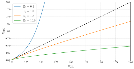
Figure 1: The redshift $z_{\rm MG}$ of a source inferred from a measurement of $d_{L}^{\,\rm gw}$ in a modified gravity model, for different values of $\Xi_{0}$, as a function of the value $z_{\rm GR}$ that would be inferred in GR (we set for definiteness $n=1.91$).

The very small redshift of GW170817, $z\simeq 0.01$, is the main limiting factor of these studies. The situation, however, can change significantly for standard sirens at higher redshifts, although still in the range accessible to 2G detectors. This can be appreciated from Fig. 1. In this plot $z_{\rm MG}$ is defined as the redshift of the source that would be inferred from a measurement of $d_{L}^{\,\rm gw}$ obtained by GW observations, using a modified gravity model with a given value of $\Xi_{0}$. We show it as a function of $z_{\rm GR}$, which is the redshift that would be inferred using GR (and $\Lambda$CDM). To produce this plot we have assumed that the corresponding electromagnetic luminosity distances are the same, in order to single out the effect of $\Xi_{0}$ [for definiteness, we set $n=1.91$, as above, but the results vary little with $n$, for $n={\cal O}(1)$]. In any case, as we discussed above, for viable models the electromagnetic luminosity distance cannot differ from that of $\Lambda$CDM by more than a few percent, which is very small with respect to the effect induced by the values of $\Xi_{0}$ shown in the plot. From Fig. 1 (that, for illustration, includes also very high and very low values of $\Xi_{0}$, such as $\Xi_{0}=0.1$ or $\Xi_{0}=10$, well beyond even those obtained in the RT model or in any other known viable model, but which can be considered at the level of a first phenomenological analysis) we see that, if the actual theory describing Nature is a modified gravity model with $\Xi_{0}>1$, the actual redshift of the source would be smaller than that inferred from the GW data using $\Lambda$CDM and, vice versa, for $\Xi_{0}<1$ it would be larger. Even without using extreme values such as $\Xi_{0}=10$ or $\Xi_{0}=0.1$, the effect can be quite significant, as long as the sources are at sufficiently large redshift.

As an example, consider the event GW190814, resulting from the coalescence of $23M_{\odot}$ BH with a compact object with a mass $2.6M_{\odot}$ [68]. Its measured (GW) luminosity distance is $d_{L}^{\,\rm gw}=241^{+41}_{-45}$ Mpc. In $\Lambda$CDM, using $H_{0}=67.9$ and $\Omega_{M}=0.30$, this gives

$$z=0.052^{+0.009}_{-0.010}\,.$$ (2.13)

Given that this redshift is still quite small, in this case the effect of modified GW propagation will not be large. Using again $H_{0}=67.9$ and $\Omega_{M}=0.30$, but setting now $\Xi_{0}=1.80$, we get

$$z=0.049^{+0.008}_{-0.008}\,,$$ (2.14)

which is not distinguishable from the GR prediction, within the error. Consider, however, a source at a larger distance, say $d_{L}^{\,\rm gw}=2920$ Mpc. In $\Lambda$CDM, with the above values of $H_{0}$ and $\Omega_{M}$, this corresponds to $z=0.50$. In contrast, in a model with the same values of $H_{0}$ and $\Omega_{M}$ but $\Xi_{0}=1.80$ (as the RT model with a large value of a parameter $\Delta N$, discussed in sect. 2.4 below), the prediction for the redshift of the source would rather be $z=0.38$, a rather significant difference; similarly, for a source at $d_{L}^{\,\rm gw}=6812$ Mpc, for which GR would predict $z=1.0$, the same modified gravity model would predict $z=0.71$. Of course, increasing the distance to the source, the average error on the measurement of the luminosity distance also increases, in a way that depends on the GW detector network under consideration, and this must be taken into account in the above considerations. In any case, in particular for the sources with the best distance reconstruction, looking for the electromagnetic counterpart by assuming a priori the validity of $\Lambda$CDM could lead to missing a possible electromagnetic counterpart. Given that the most important outcome of these observations would be a possible falsification of $\Lambda$CDM and of GR, it is important to extend the search for a counterpart to a range of redshifts not limited to that predicted by $\Lambda$CDM.

The predictions for the redshift of the source, which can discriminate between GR and modified gravity theories, can be tested either using standard sirens with counterpart, or using dark sirens. On the counterpart side, we have seen above that GW170817 is too close to give stringent results. For the BBH GW190521 a tentative electromagnetic counterpart, ZTF19abanrhr, has been reported in [70], although, using $\Lambda$CDM as the underlying cosmological model, the probability of a real association based on volume localization is not statistically sufficient for a confident identification of ZTF19abanrhr as the counterpart [71]. Furthermore, uncertainties exist about the physical mechanism providing a flare from the coalescence of the BBH, believed to have taken place in a AGN disk. However, this event is the furthest detection reported by LIGO/Virgo in the O3a run, at $d_{L}^{\,\rm gw}\sim(4-5)$ Gpc, and it is therefore very interesting from the point of view of modified GW propagation. We will examine it in sect. 4.3 (see also the related analysis in [72]), where we will also see that modified GW propagation could remove a significant objection to the interpretation of ZTF19abanrhr as a counterpart, namely the limited spatial localization overlap of the GW and electromagnetic signals. Most of our results, however, will be focused on the measurement that can be obtained with current dark sirens observations, both for $H_{0}$ and for $\Xi_{0}$.

2.4 An explicit example: the RT nonlocal model

Our analysis of modified GW propagation, in this paper, will be of purely phenomenological nature: we will assume a modified gravity model with a prediction for the ‘electromagnetic’ luminosity distance very close to that of $\Lambda$CDM (say, at a few percent or better, so that, at the level of the present analysis, we will neglect this difference) and, on top of it, a much larger effect due to modified GW propagation, parametrized in terms of $(\Xi_{0},n)$ with a value of $\Xi_{0}$ significantly different from 1. To support the potential interest of this phenomenological scenario, it is useful to have in mind an explicit model that realizes it, even if, in the end, our analysis will be more general.

An explicit realization of this scenario is provided by the ‘RT’ nonlocal gravity model. This model was originally proposed in [73], and has been much explored by our group in recent years. A complete and updated review of its conceptual and phenomenological aspects can be found in [61] (which updates the review [74]), whom we refer the reader for more details. In short, the underlying idea is that, because of infrared effects in spacetimes of cosmological interest, the conformal mode of the metric becomes massive, and this is described by the generation of a suitable non-local term in the quantum effective action. Various studies of this model and of variants of the same underlying physical idea [75, 76, 77, 78, 79, 80, 81, 82, 74, 83, 84, 85] have shown that the model passes all phenomenological constraints: it generates dynamically a dark energy density that drives accelerated expansion in the recent epoch; it has stable cosmological perturbations in the scalar and tensor sectors (a nontrivial condition that ruled out many modified gravity models even before reaching the stage of comparison with data); the model fits CMB, BAO, SNe and structure formation at a level statistically equivalent to $\Lambda$CDM; and it reproduces the successes of GR at solar system scale, including bounds on the time variation of Newton’s constant, and laboratory scales (without the need of a screening mechanism since, contrary to all other modifications of GR, it does not introduce extra degrees of freedom). Studies of possible variations of the idea have singled out the RT model as the only known nonlocal model that passes all these tests.

The fact that the RT model passes all phenomenological tests is partly related to the fact that it differs from $\Lambda$CDM by less that $0.5\%$ at the level of background evolution and by a few percent to below percent level, depending on the wavenumber of the Fourier modes, for the scalar perturbations (see e.g. Fig. 2 and Figs. 5-14 of [61]). In the tensor sector, one finds that GWs propagate at the speed of light, therefore complying with the bound from GW170817, and the model displays the phenomenon of modified GW propagation. Quite surprisingly, despite the fact that the model is so close to $\Lambda$CDM at the background level and in the scalar perturbations, the deviations from GR in the tensor sector, as parametrized by $\Xi_{0}$, can be very large [60, 61]. More precisely, the model has a free parameter $\Delta N$, related to the choice of initial conditions (defined by starting the evolution during a phase of primordial inflation, $\Delta N$ e-folds before the end of inflation) and, for large $\Delta N$, the prediction for $\Xi_{0}$ of the RT model saturates to a value $\Xi_{0}\simeq 1.80$, corresponding to a $80\%$ deviation from the GR value $\Xi_{0}=1$. In contrast, if the model is started with initial conditions of order one during radiation dominance, one rather finds $\Xi_{0}\simeq 0.93$, a $7\%$ deviation from GR.

Apart from its specific virtues as a viable dynamical dark energy model, the RT model therefore provides an explicit example of a phenomenologically viable modification of GR that produces very large deviations from GR in the sector of tensor perturbations. This shows how the study of GWs on cosmological scales is a genuinely new window, accessible only to GW detectors, that has the potential of providing significant surprises.

3 Methodology for correlation between dark sirens and galaxy catalogs

We now move to the study of standard sirens without electromagnetic counterpart (‘dark sirens’), using a statistical method based on the correlation with a galaxy catalog. In this section, we will give a detailed discussion of the methodology used, and we suggest various improvements with respect to the current state of the art.

3.1 Hierarchical Bayesian framework

We use a hierarchical Bayesian statistical framework, elaborating on the formalism discussed in refs. [87, 15]. This formalism has been recently used for extracting $H_{0}$ from various LIGO/Virgo detections discussed in the Introduction (in [31] for GW170817 without using the known electromagnetic counterpart, in [32] for GW170814 and in [33] for GW190814). A related formalism is discussed in [17] and has been used by the LIGO/Virgo collaboration for extracting a value of $H_{0}$ from the detections of the O1 and O2 observation runs [34], and in [68, 88] for GW190814. See also [89, 13, 90] for earlier work on applications of the hierarchical Bayesian method to astrophysics, and [91, 92] for reviews.

We consider an ensemble of binary coalescences, each characterized by a set of parameters $\theta$ that determine the GW signal. Among them, we separate the position of the source from the other parameters. The position can be described by its luminosity distance $d_{L}$ and by its direction, identified by a unit vector $\hat{\Omega}$, so we write

$$\theta=\{d_{L},\hat{\Omega},\theta^{\prime}\}\,.$$ (3.1)

Equivalently, given a cosmology, we can use the redshift $z$ instead of the luminosity distance $d_{L}$, so $\theta=\{z,\hat{\Omega},\theta^{\prime}\}$. Note also that, in the context of modified gravity, the quantity directly measured by the GW signal is the GW luminosity distance $d_{L}^{\,\rm gw}$, rather than the electromagnetic luminosity distance $d_{L}^{\,\rm em}\equiv d_{L}$. In any case, the actual position of the source is given by the electromagnetic luminosity distance $d_{L}$. The set $\theta^{\prime}$ contains all other source parameters that affect the GW signal. Among them, the most important are the chirp mass and the total mass of the system, and the inclination of the orbit, but at higher and higher level of accuracy other parameters will enter, such as the spins of the compact bodies, tidal deformability in the case of a NS, eccentricity of the orbit, etc.

We collectively denote by $\lambda$ the set of parameters on which we want to draw an inference from the set of measurements of binary coalescences. These could be properties of the underlying astrophysical population, such as their rate of coalescence or their mass distribution, as well as parameters of the underlying cosmological model, such as $H_{0}$ or, in the context of modified gravity, $\Xi_{0}$. As in ref. [87], we separate $\lambda$ into an overall normalization for the event rate $N$ (that will be treated separately, see sect. 3.4) and the remaining parameters, denoted by $\lambda^{\prime}$, so $\lambda=\{N,\lambda^{\prime}\}$. The distribution $dN/d\theta$ of the events (in our case, the GW events due to binary coalescences) is written as

$$\frac{dN}{d\theta}(\lambda)=Np_{0}(\theta|\lambda^{\prime})\,.$$ (3.2)

When we study the Hubble parameter in the context of $\Lambda$CDM we fix all parameters related to the underlying astrophysical population to typical values suggested by astrophysical models (we will then explore the effect of different choices) and we keep all other cosmological parameters fixed to the mean values obtained from CMB+BAO+SNe, so $\lambda^{\prime}=\{H_{0}\}$. This is the strategy that has been used also in [31, 32]. In principle, we should also allow $\Omega_{M}$, which is the other relevant cosmological parameter that enters in eq. (1.1), to vary within a prior fixed by CMB+BAO+SNe data. However, the latter fix $\Omega_{M}$ to an accuracy of order $2\%$, which, as we shall see, is much better than what we will obtain for $H_{0}$ using only standard sirens. Then, to the level of accuracy that can be currently reached, it is sensible to keep $\Omega_{M}$ fixed.^, More generally, one could perform a global fit inferring both the cosmology and the population properties. This is particularly useful when some feature of the population property, such as the narrowness of the neutron star mass distribution [93], or the mass scale that can be imprinted on the BH mass distribution by the pulsational pair-instability supernova mechanism [53], can break the degeneracy between source frame masses and redshifts, thereby providing independent statistical information of the redshift (see also [94] for a recent discussion of the interplay between population property and cosmological parameters inference). In this paper we will limit ourselves to inference of the cosmological parameters, for fixed choices of astrophysical population properties, and we will examine how the results depends on the assumed population properties.

Similarly, when we study modified GW propagation, we keep $\Xi_{0}$ as the only free parameter and we fix all other cosmological parameters, including $H_{0}$, to the mean values obtained from CMB+BAO+SNe, so $\lambda^{\prime}=\{\Xi_{0}\}$. Once again, rather than fixing them, in principle one should vary all other cosmological parameters within a prior fixed by CMB+BAO+SNe data. However, given that current CMB+BAO+SNe data fix $H_{0}$ to an accuracy of about $0.7\%$ [21], while the bounds that we will find on $\Xi_{0}$ from dark sirens will turn out to be about two orders of magnitude less constraining, with current GW data keeping $H_{0}$ fixed to the mean value obtained from CMB+BAO+SNe is again an adequate approximation. As the amount and quality of GW data will improve, this will no longer be appropriate. Actually, at the level of 3G detectors, when are expected millions of BBH detections per year [55], it would not even be appropriate to separate electromagnetic from GW data, using only the former to determine the prior on $H_{0}$ and the other cosmological parameters, and then using GW data to study $\Xi_{0}$, with the other parameters allowed to vary within these priors. Rather, the best approach will be to run full MCMCs on the whole electromagnetic+GW datasets, as done in [36] with simulated ET data and in [48] with simulated LISA data. Eventually, especially in view of the $H_{0}$ tension between early- and late-Universe probes, one would also like to have a joint measurement of $(H_{0},\Xi_{0})$ from standard sirens only, without using electromagnetic data at all. However, to achieve this with sufficient accuracy will be challenging even for a 3G detector such as ET, see Fig. 13 of [36]. At present, given the limited constraining power on the cosmological parameters of current GW data, the approach that we take in this work, of fixing all parameters except $H_{0}$ when we study $H_{0}$ within $\Lambda$CDM, and all parameters (including $H_{0}$) except $\Xi_{0}$ when we study modified GW propagation, is adequate.

The distribution (3.2) is sampled with a set $\{{\cal D}_{\rm GW}\}$ of $N_{\rm obs}$ observations of binary coalescences, each one providing GW data ${\cal D}_{\rm GW}^{i}$, $i=1,\ldots,N_{\rm obs}$, and we assume that there is no electromagnetic counterpart, i.e. no corresponding electromagnetic data. As in [87], we begin by focusing on the possibility of extracting information on the parameters $\lambda^{\prime}$ (we will later specify our notation to $\lambda^{\prime}=\{H_{0}\}$ or to $\lambda^{\prime}=\{\Xi_{0}\}$, depending on the context. In this section, however, we still use the more general notation $\lambda^{\prime}$). The posterior for $\lambda^{\prime}$, given the GW data, is obtained from

$$p(\lambda^{\prime}|\{{\cal D}_{\rm GW}\})=\frac{p(\{{\cal D}_{\rm GW}\}|\lambda^{\prime})\,\pi(\lambda^{\prime})}{p(\{{\cal D}_{\rm GW}\})}\,,$$ (3.3)

where $p(\{{\cal D}_{\rm GW}\}|\lambda^{\prime})$ is the likelihood of the data given $\lambda^{\prime}$, and $\pi(\lambda^{\prime})$ is the prior on $\lambda^{\prime}$. Both for $\lambda^{\prime}=\{H_{0}\}$ and for $\lambda^{\prime}=\{\Xi_{0}\}$ we will use a flat prior within broad limits, see below. The probability of the data $p(\{{\cal D}_{\rm GW}\})$ (the ‘evidence’) ensures the normalization $\int d\lambda^{\prime}\,p(\lambda^{\prime}|\{{\cal D}_{\rm GW}\})=1$, so

$$p(\{{\cal D}_{\rm GW}\})=\int d\lambda^{\prime}\,p(\{{\cal D}_{\rm GW}\}|\lambda^{\prime})\,\pi(\lambda^{\prime})\,,$$ (3.4)

and is therefore independent of $\lambda^{\prime}$. For a set $\{{\cal D}_{\rm GW}\}$ of $N_{\rm obs}$ independent detections (neglecting for the moment the information on the overall rate, see sect. 3.4), the total likelihood is given by

$$p(\{{\cal D}_{\rm GW}\}|\lambda^{\prime})=\prod_{i=1}^{N_{\rm obs}}p({\cal D}^{i}_{\rm GW}|\lambda^{\prime})\,.$$ (3.5)

The likelihood $p({\cal D}^{i}_{\rm GW}|\lambda^{\prime})$ of the $i$-th GW event can be written as [87]

$$p({\cal D}^{i}_{\rm GW}|\lambda^{\prime})=\frac{1}{\beta(\lambda^{\prime})}\int d\theta\,p({\cal D}^{i}_{\rm GW}|\theta,\lambda^{\prime})\,p_{0}(\theta|\lambda^{\prime})\,,$$ (3.6)

where $p({\cal D}^{i}_{\rm GW}|\theta,\lambda^{\prime})$ is the likelihood of the data ${\cal D}^{i}_{\rm GW}$ given the value $\theta$ of the parameters, and $p_{0}(\theta|\lambda^{\prime})$, defined by eq. (3.2), is the prior on the parameters $\theta$. Both are in principle conditioned on $\lambda^{\prime}$, although this depends on the choice of the variables $\theta$, as we will see below. The qualification ‘hierarchical’ Bayesian inference refers to the fact that, through the data, we do not have access directly to $\lambda^{\prime}$ but rather to the posterior of the parameters $\theta$ given the data, and therefore, through Bayes’ theorem, to the likelihood $p({\cal D}^{i}_{\rm GW}|\theta,\lambda^{\prime})$. The desired likelihood with respect to the parameters $\lambda^{\prime}$ is then obtained using eq. (3.6) [and the corresponding posterior from eq. (3.3)]. In this context the parameters $\lambda^{\prime}$ (or, more generally, $\lambda$, including the overall rate) are often called hyper-parameters, and $p(\{{\cal D}_{\rm GW}\}|\lambda)$ is called the hyper-likelihood.

In our problem, when $\theta=\{d_{L},\hat{\Omega}\}$, the prior $p_{0}(\theta|\lambda^{\prime})$ will be provided by the galaxy catalog, with the precise connection discussed in sect. 3.2. We will then discuss how to include the prior on the remaining parameters $\theta^{\prime}$.

The function $\beta(\lambda^{\prime})$ is a normalization factor, that ensures that the integral of $p({\cal D}^{i}_{\rm GW}|\lambda^{\prime})$ over all data above the detection threshold is equal to one, so [87]

$$\beta(\lambda^{\prime})=\int_{{\cal D}_{\rm GW}>{\rm threshold}}d{\cal D}_{\rm GW}\,\int d\theta\,p({\cal D}_{\rm GW}|\theta,\lambda^{\prime})\,p_{0}(\theta|\lambda^{\prime})\,.$$ (3.7)

We can rewrite this expression as

$$\beta(\lambda^{\prime})=\int d\theta\,P_{\rm det}(\theta,\lambda^{\prime})\,p_{0}(\theta|\lambda^{\prime})\,,$$ (3.8)

where

$$P_{\rm det}(\theta,\lambda^{\prime})\equiv\int_{{\cal D}_{\rm GW}>{\rm threshold}}d{\cal D}_{\rm GW}\,p({\cal D}_{\rm GW}|\theta,\lambda^{\prime})\,$$ (3.9)

is the detection probability for a source characterized by the parameters $\theta$, for the given $\lambda^{\prime}$. The normalization factor $\beta(\lambda^{\prime})$ represents the fraction of events that can be detected, in a population characterized by the distribution $p_{0}(\theta|\lambda^{\prime})$. As stressed in [87, 15, 31], since this normalization factor depends on $\lambda^{\prime}$, we must include its dependence in order to obtain the correct likelihood and indeed, as we will see, it is quite crucial to compute it accurately to obtain meaningful results.

Putting together eqs. (3.5) and (3.6), in the approximation in which we neglect the information on the total rate, we have

$$p(\{{\cal D}_{\rm GW}\}|\lambda^{\prime})=\,\frac{1}{[\beta(\lambda^{\prime})]^{N_{\rm obs}}}\,\prod_{i=1}^{N_{\rm obs}}\int d\theta\,p({\cal D}^{i}_{\rm GW}|\theta,\lambda^{\prime})\,p_{0}(\theta|\lambda^{\prime})\,,$$ (3.10)

with $\beta(\lambda^{\prime})$ given by eqs. (3.8) and (3.9).

The hierarchical Bayesian framework has been first developed to study the hyper-parameters $\lambda$ that characterize the underlying astrophysical population, see e.g. [90, 87, 91, 92]. In that case (with a natural choice for the parameters $\theta$, see below), the hyper-parameters $\lambda^{\prime}$ (or, more, generally, $\lambda$) only affect $p_{0}(\theta|\lambda^{\prime})$, which encodes the information on the population, and do not enter in $p({\cal D}^{i}_{\rm GW}|\theta,\lambda^{\prime})$, which can therefore be written simply as $p({\cal D}^{i}_{\rm GW}|\theta)$. As an example, the hyper-parameters could describe the shape of the mass function of the BH masses in a BH-BH binary. These parameters enter in the description of the population, i.e. in $p_{0}(\theta|\lambda^{\prime})$; however, the probability of detection is uniquely fixed in terms of the parameters $\theta$, e.g. the distance, masses, etc. of the specific event. The formalism, however, can be extended to the case where $\lambda^{\prime}$ include also cosmological parameters such as $H_{0}$. In this case, in general, $\lambda^{\prime}$ also enters in $p({\cal D}^{i}_{\rm GW}|\theta,\lambda^{\prime})$. More precisely, the conditioning on $\lambda^{\prime}$, in eq. (3.10), depends on the choice of the variables $\theta$. Indeed, suppose that we start from variables $\theta$ such that $p({\cal D}_{\rm GW}|\theta,\lambda^{\prime})$ is independent of $\lambda^{\prime}$, so

$$p({\cal D}^{i}_{\rm GW}|\lambda^{\prime})=\frac{1}{\beta(\lambda^{\prime})}\int d\theta\,p({\cal D}^{i}_{\rm GW}|\theta)\,p_{0}(\theta|\lambda^{\prime})\,.$$ (3.11)

One might then wish to make a transformation to new variables

$$\theta\rightarrow\tilde{\theta}(\theta,\lambda^{\prime})\,,$$ (3.12)

which involves the hyper-parameters $\lambda^{\prime}$. Such a transformation would be possible, in principle, even when $\lambda^{\prime}$ only describe the astrophysical population, but in that case it would be very unnatural. In contrast, we will see on some explicit examples below that it can be very natural when the hyper-parameters describe the cosmological model. Under this transformation

$$p_{0}(\theta|\lambda^{\prime}) \rightarrow \tilde{p}_{0}(\tilde{\theta}|\lambda^{\prime})=p_{0}(\theta(\tilde{\theta},\lambda^{\prime})|\lambda^{\prime})\frac{d\theta}{d\tilde{\theta}}\,,$$ (3.13)

$$p({\cal D}_{\rm GW}|\theta) \rightarrow \tilde{p}({\cal D}_{\rm GW}|\tilde{\theta},\lambda^{\prime})=p({\cal D}_{\rm GW}|\theta(\tilde{\theta},\lambda^{\prime}))\,.$$ (3.14)

These are the correct transformation laws for these quantities, since $p_{0}(\theta|\lambda^{\prime})$ is a probability distribution with respect to $\theta$, so $\tilde{p}_{0}(\tilde{\theta}|\lambda^{\prime})d\tilde{\theta}=p_{0}(\theta|\lambda^{\prime})d\theta$, while $p({\cal D}_{\rm GW}|\theta,\lambda^{\prime})$ is rather a probability distribution with respect to ${\cal D}_{\rm GW}$ and is a ‘scalar’ with respect to transformations of the $\theta$ variables. This transformation therefore induces a dependence on the hyper-parameters in $\tilde{p}({\cal D}_{\rm GW}|\tilde{\theta},\lambda^{\prime})$, even if it was absent in $p({\cal D}_{\rm GW}|\theta)$.

As an example, consider the case where we want to infer the value of $H_{0}$ within $\Lambda$CDM, so that $\lambda^{\prime}=\{H_{0}\}$, and we chose as variables $\theta=\{d_{L},\hat{\Omega},\theta^{\prime}\}$, where $d_{L}$ is the standard luminosity distance in GR. Then eq. (3.6) reads

$$p({\cal D}^{i}_{\rm GW}|H_{0})=\frac{1}{\beta(H_{0})}\int d(d_{L})d\Omega d\theta^{\prime}\,p({\cal D}^{i}_{\rm GW}|d_{L},\hat{\Omega},\theta^{\prime})\,p_{0}(d_{L},\hat{\Omega},\theta^{\prime}|H_{0})\,,$$ (3.15)

and

$$\beta(H_{0})=\int d(d_{L})d\Omega d\theta^{\prime}\,P_{\rm det}(d_{L},\hat{\Omega},\theta^{\prime})\,p_{0}(d_{L},\hat{\Omega},\theta^{\prime}|H_{0})\,.$$ (3.16)

Note that the GW measurement is sensitive directly to the luminosity distance $d_{L}$ and the direction $\hat{\Omega}$ of the source, so $p({\cal D}^{i}_{\rm GW}|d_{L},\hat{\Omega},\theta^{\prime})$ is independent of $H_{0}$. In contrast, the galaxy radial positions are first obtained by measuring their redshifts, which can then be translated into values for $d_{L}$ by making use of $H_{0}$. Therefore, the term $p_{0}(d_{L},\hat{\Omega},\theta^{\prime}|H_{0})$ depends on $H_{0}$. The choice $\theta=\{d_{L},\hat{\Omega},\theta^{\prime}\}$ is therefore an example of a choice of variables such that the dependence on the hyper-parameters is only in $p_{0}(\theta|\lambda^{\prime})$.

We could, however, equally well choose as variables $\theta=\{z,\hat{\Omega},\theta^{\prime}\}$, so that both the radial position of the GW event and of the galaxies are expressed in terms of the redshift $z$ (this is indeed the choice made in [15, 31, 32]). In this case, eq. (3.15) is replaced by

$$p({\cal D}^{i}_{\rm GW}|H_{0})=\frac{1}{\beta(H_{0})}\int dzd\Omega d\theta^{\prime}\,p({\cal D}^{i}_{\rm GW}|d_{L}(z,H_{0}),\hat{\Omega},\theta^{\prime})\,p_{0}(z,\hat{\Omega},\theta^{\prime})\,.$$ (3.17)

Note that now, in eq. (3.17), the dependence on $H_{0}$ has been entirely moved from the prior to the likelihood. In fact, the galaxy catalog is obtained directly in redshift space, so the probability density for finding a galaxy in the catalog at a given $z$, expressed by the prior $p_{0}(z,\hat{\Omega},\theta^{\prime})$, is independent of $H_{0}$. In contrast, the probability of the GW data ${\cal D}^{i}_{\rm GW}$ depends on the luminosity distance of the source, and can be expressed as a function of redshift through the function $d_{L}(z,H_{0})$, that carries the dependence on $H_{0}$.

Another option, for example, could be to use comoving coordinates ${\bf x}$, with $|{\bf x}|\equiv d_{\rm com}$. In that case, both $p({\cal D}^{i}_{\rm GW})$ and $p_{0}$ would depend on $H_{0}$, since $H_{0}$ (and, more generally, the cosmology) enters both in the transformation from $z$ to $d_{\rm com}$ and in the transformation from $d_{L}$ to $d_{\rm com}$ (although, for close sources, the latter dependence disappears and $d_{L}\simeq d_{\rm com}$).

In the following, to make easier the comparison with refs. [15, 31, 32], we will use $\{z,\hat{\Omega}\}$. Observe also that the normalization constant $\beta(\lambda^{\prime})$ is invariant under the transformation (3.12)–(3.14), as we see inserting eqs. (3.13) and (3.14) into eqs. (3.8) and (3.9).

From the above discussion, we see that there are three main ingredients in the formalism: the first is the probability of the GW data given the parameters of the source and the hyper-parameters $\lambda^{\prime}$, $p({\cal D}^{i}_{\rm GW}|\theta,\lambda^{\prime})$. For the study of $H_{0}$ or of $\Xi_{0}$ we are interested mostly in the distance and direction to the GW event. In this case a useful approximation is obtained assuming a gaussian likelihood with direction-dependent parameters [95, 96],

$${\cal L}_{i}(d_{L},\hat{\Omega})\equiv p({\cal D}^{i}_{\rm GW}|d_{L},\hat{\Omega})=\rho_{i}(\hat{\Omega})\,\frac{{\cal N}_{i}(\hat{\Omega})}{\sqrt{2\pi}\,\sigma_{i}(\hat{\Omega})}\,\exp\left\{-\frac{[d_{L}-\mu_{i}(\hat{\Omega})]^{2}}{2\sigma_{i}^{2}(\hat{\Omega})}\right\}\,.$$ (3.18)

The quantities $\rho_{i}(\hat{\Omega})$, ${\cal N}_{i}(\hat{\Omega})$, $\sigma_{i}(\hat{\Omega})$ and $\mu_{i}(\hat{\Omega})$ for the $i$-th GW event are provided by the LIGO/Virgo skymaps, for a discrete set of values of $\hat{\Omega}$ corresponding to the HEALPix pixelization [97]. The corresponding posterior distribution of $d_{L}$, conditional on the direction $\hat{\Omega}$, is given by

$$p(d_{L}|\hat{\Omega})d(d_{L})=\frac{{\cal N}_{i}(\hat{\Omega})}{\sqrt{2\pi}\,\sigma_{i}(\hat{\Omega})}\,\exp\left\{-\frac{[d_{L}-\mu_{i}(\hat{\Omega})]^{2}}{2\sigma_{i}^{2}(\hat{\Omega})}\right\}\,\pi(d_{L})d(d_{L})\,.$$ (3.19)

The term $\pi(d_{L})$ is the prior chosen by the LIGO/Virgo collaboration to obtain the posterior. For our purposes we only need the likelihood (3.18), which we obtain from the publicly available posteriors by removing the prior $\pi(d_{L})\propto d_{L}^{2}$ that has been used by the LIGO/Virgo collaboration. The factor ${\cal N}_{i}(\hat{\Omega})$ is a normalization constant, given for convenience, fixed by the condition

$$\int_{0}^{\infty}d(d_{L})\,p(d_{L}|\hat{\Omega})=1\,,$$ (3.20)

so that $p(d_{L}|\hat{\Omega})$ is a normalized pdf. The remaining overall factor $\rho_{i}(\hat{\Omega})$ in eq. (3.18) then gives the probability that the event is in the direction $\hat{\Omega}$. As discussed in [95, 96], eq. (3.19) provides a good approximation to the full posterior (conditional on $\hat{\Omega}$) obtained from the MCMC.

For the case of $H_{0}$, the likelihood can be written as a function of $z$ as

$${\cal L}_{i}(z,\hat{\Omega},H_{0})=\rho_{i}(\hat{\Omega})\,\frac{{\cal N}_{i}(\hat{\Omega})}{\sqrt{2\pi}\,\sigma_{i}(\hat{\Omega})}\,\exp\left\{-\frac{[d_{L}(z,H_{0})-\mu_{i}(\hat{\Omega})]^{2}}{2\sigma_{i}^{2}(\hat{\Omega})}\right\}\,.$$ (3.21)

Similarly, for modified gravity,

$${\cal L}_{i}(z,\hat{\Omega},\Xi_{0})\equiv p({\cal D}^{i}_{\rm GW}|d_{L}^{\,\rm gw}(z,\Xi_{0}),\hat{\Omega})=\rho_{i}(\hat{\Omega})\,\frac{{\cal N}_{i}(\hat{\Omega})}{\sqrt{2\pi}\,\sigma_{i}(\hat{\Omega})}\,\exp\left\{-\frac{[d_{L}^{\,\rm gw}(z,\Xi_{0})-\mu_{i}(\hat{\Omega})]^{2}}{2\sigma_{i}^{2}(\hat{\Omega})}\right\}\,.$$ (3.22)

In this work, we will always use the publicly available gaussian likelihoods (3.18).

The second ingredient is the prior $p_{0}(z,\hat{\Omega},\theta^{\prime})$. For $\{z,\hat{\Omega}\}$, this will be obtained from a galaxy catalog. This entails the physical assumption that the spatial location of BH-BH coalescences is correlated with the position of galaxies. This is a natural assumption for BHs of astrophysical origin, but might not be true if most of the BHs in the observed coalescences were of primordial, rather than astrophysical, origin. As stressed in [15, 31, 17], the issue of completeness of the catalog introduces some delicate aspects, that we will discuss in sect. 3.2.

Finally, the third ingredient is the computation of the normalization factor, $\beta(H_{0})$ or $\beta(\Xi_{0})$. When using $z$ as variable, the expression for $\beta(H_{0})$ is given by

$$\beta(H_{0})=\int dzd\Omega d\theta^{\prime}\,P_{\rm det}[d_{L}(z,H_{0}),\hat{\Omega},\theta^{\prime}]\,p_{0}(z,\hat{\Omega},\theta^{\prime})\,,$$ (3.23)

where, again, we used the fact that the, in $P_{\rm det}$, the dependence on $z$ and $H_{0}$ enters through $d_{L}(z,H_{0})$ (see, however, footnote 12). When we study modified GW propagation, we rather have

$$\beta(\Xi_{0})=\int dzd\Omega d\theta^{\prime}\,P_{\rm det}[d_{L}^{\,\rm gw}(z,\Xi_{0}),\hat{\Omega},\theta^{\prime}]\,p_{0}(z,\hat{\Omega},\theta^{\prime})\,.$$ (3.24)

The computation of these normalization factors therefore involves a model for the detection process, and will be discussed in sect. 3.3, where we will elaborate and improve on the computation in refs. [15, 31].

3.2 The $p_{0}(z,\hat{\Omega})$ prior: galaxy catalogs and completeness

We now assume that the prior $p_{0}(z,\hat{\Omega},\theta^{\prime})$ factorizes as

$$p_{0}(z,\hat{\Omega},\theta^{\prime})=p_{0}(z,\hat{\Omega})\tilde{p}_{0}(\theta^{\prime})\,,$$ (3.25)

and we separately normalize

$$\int dzd\Omega\,p_{0}(z,\hat{\Omega})=1\,,$$ (3.26)

and

$$\int d\theta^{\prime}\,\tilde{p}_{0}(\theta^{\prime})=1\,.$$ (3.27)

At some level of accuracy this factorization assumption will have to be improved since, for instance, the distribution of masses in a binary black hole (BBH) might be correlated with redshift (see [98] for a recent discussion in the context of the GWTC-2 catalog). However, this factorization is a sensible starting point. We will later improve this prior by including a parametrization of the redshift dependence of the BBH merger rate, see eq. (3.45) below.

To determine the prior $p_{0}(z,\hat{\Omega})$ we use the public GLADE galaxy catalog (v2.4) [99] (http://glade.elte.hu) because of its full sky coverage. When using a galaxy catalog, completeness is a crucial issue. In an ideal complete catalog, the prior would simply be given by $p_{0}(z,\hat{\Omega})=p_{\rm cat}(z,\hat{\Omega})$, where

$$p_{\rm cat}(z,\hat{\Omega})=\frac{\sum_{\alpha=1}^{N_{\rm cat}}w_{\alpha}\delta(z-z_{\alpha})\delta^{(2)}(\hat{\Omega}-\hat{\Omega}_{\alpha})}{\sum_{\alpha=1}^{N_{\rm cat}}w_{\alpha}}\,.$$ (3.28)

Here $N_{\rm cat}$ is the number of galaxies in the catalog, $z_{\alpha}$ are the cosmological redshifts of the galaxies (obtained correcting the measured redshift for peculiar velocities) and $\hat{\Omega}_{\alpha}$ their directions. Note that we use the index $i$ to label the GW events, and $\alpha$ to label the galaxies. Here we have assumed that the errors on $z_{\alpha},\hat{\Omega}_{\alpha}$ are negligible with respect to the corresponding errors of the GW events. This is an excellent approximation for $\hat{\Omega}_{\alpha}$, compared to the current and future angular resolution of GW detector networks. For the redshift this is not always a good approximation, particularly for galaxies with photometric redshift determination, and can be improved by replacing, for each galaxy, the Dirac delta by a gaussian approximation to the $z_{\alpha}$ posterior, as in [31], so that

$$p_{\rm cat}(z,\hat{\Omega})=\frac{\sum_{\alpha=1}^{N_{\rm cat}}w_{\alpha}{\cal N}(z;z_{\alpha},\sigma_{\alpha})\delta^{(2)}(\hat{\Omega}-\hat{\Omega}_{\alpha})}{\sum_{\alpha=1}^{N_{\rm cat}}w_{\alpha}}\,,$$ (3.29)

where ${\cal N}(z;z_{\alpha},\sigma_{\alpha})$ is a gaussian pdf in the variable $z$, with mean $z_{\alpha}$ and variance $\sigma_{\alpha}$. In particular, for the GLADE catalog, the likelihoods are taken to be gaussian with a width $\Delta z\simeq 1.5\times 10^{-4}$ for galaxies with spectroscopic redshift and $\Delta z\simeq 1.5\times 10^{-2}$ for galaxies with photometric redshift [99]. More generally, one could actually use the full posterior of the redshift distribution of each galaxy. This is obtained multiplying the likelihood (that need not be gaussian) by a prior, which is naturally chosen as a volume prior $dV_{c}/dz$, where $V_{c}$ is the comoving volume (followed by normalization). For narrow, gaussian likelihoods, such as in GLADE, these posteriors are well fitted by another gaussian, that, eventually, is the quantity that we denote by ${\cal N}(z;z_{\alpha},\sigma_{\alpha})$ in eq. (3.29). However, our code can treat the general case, see also footnote 31 on page 31. In the formulas below, for notational simplicity, we simply write $\delta(z-z_{\alpha})$, but all these formulas are trivially generalized replacing $\delta(z-z_{\alpha})$ by the full posterior for the redshifts.

In eq. (3.29) we have inserted the normalization factor $\sum_{\alpha=1}^{N_{\rm gal}}w_{\alpha}$ at the denominator, so that $p_{\rm cat}(z,\hat{\Omega})$ is a properly normalized pdf,

$$\int dzd\Omega\,p_{\rm cat}(z,\hat{\Omega})=1\,.$$ (3.30)

The factors $w_{\alpha}$ allow for the possibility of weighting differently the probability that a galaxy is the host of a given GW signal. As in [31], we will examine three different choices. The simplest option is to set all $w_{\alpha}=1$, corresponding to equal probability for each galaxy to host the source. Alternatively, we can weight the galaxies by their B-band luminosity $L_{B}$, which is a proxy for their star formation rate, or by their K-band luminosity $L_{K}$, which is a proxy for their total stellar mass. As we will discuss in app. A, for the GLADE catalog the most appropriate choice is to use luminosity weighting, either in the B or in the K band.

In general, however, galaxy catalogs are incomplete, especially all-sky catalogs that reach large distances. In app. A, expanding on the results presented in [99, 31], we will study the completeness of the GLADE catalog according to the measures of completeness that we develop in this section. The incompleteness of the catalog means that the simple prior $p_{0}(z,\hat{\Omega})=p_{\rm cat}(z,\hat{\Omega})$, with $p_{\rm cat}(z,\hat{\Omega})$ given by eq. (3.28), must be modified. To this purpose we consider a region ${\cal R}$, sufficiently large to include all the GW events potentially detectable by the GW detector network under consideration; typically this will be a spherical ball in redshift space, with a sufficiently large radius $z_{\cal R}$, but for the moment we keep the shape of ${\cal R}$ generic. We denote by $N_{\rm gal}({\cal R})$ the total number of galaxies in this region, by $N_{\rm cat}({\cal R})$ the number of galaxies in ${\cal R}$ that are actually present in the catalog, and by $N_{\rm miss}({\cal R})=N_{\rm gal}({\cal R})-N_{\rm cat}({\cal R})$ the number of galaxies that have been missed. The natural prior would be given by the sum over all galaxies in ${\cal R}$,

$$p_{0}(z,\hat{\Omega};{\cal R})=\frac{\sum_{\alpha=1}^{N_{\rm gal}({\cal R})}w_{\alpha}\delta(z-z_{\alpha})\delta^{(2)}(\hat{\Omega}-\hat{\Omega}_{\alpha})}{\sum_{\alpha=1}^{N_{\rm gal}({\cal R})}w_{\alpha}}\,.$$ (3.31)

(In this section we will use the notation $p_{0}(z,\hat{\Omega};{\cal R})$, where the region ${\cal R}$ is written explicitly). We can split the sum over the galaxies in ${\cal R}$ into a sum over those that are the catalog and over those that have been missed,

$$p_{0}(z,\hat{\Omega};{\cal R}) = \frac{1}{\sum_{\alpha=1}^{N_{\rm gal}({\cal R})}w_{\alpha}}\,$$

$$\times\left[\sum_{\alpha_{1}=1}^{N_{\rm cat}({\cal R})}w_{\alpha_{1}}\delta(z-z_{\alpha_{1}})\delta^{(2)}(\hat{\Omega}-\hat{\Omega}_{\alpha_{1}})+\sum_{\alpha_{2}=1}^{N_{\rm miss}({\cal R})}w_{\alpha_{2}}\delta(z-z_{\alpha_{2}})\delta^{(2)}(\hat{\Omega}-\hat{\Omega}_{\alpha_{2}})\right]\,,$$

where, for clarity, we have used the dummy index $\alpha$ for the sum over all galaxies, $\alpha_{1}$ for the sum over the galaxies in the catalog and $\alpha_{2}$ for the sum over missed galaxies. We define the normalized pdf’s

$$p_{\rm cat}(z,\hat{\Omega};{\cal R}) = \frac{\sum_{\alpha_{1}=1}^{N_{\rm cat}({\cal R})}w_{\alpha_{1}}\delta(z-z_{\alpha_{1}})\delta^{(2)}(\hat{\Omega}-\hat{\Omega}_{\alpha_{1}})}{\sum_{\alpha_{1}=1}^{N_{\rm cat}({\cal R})}w_{\alpha_{1}}}\,,$$ (3.33)

$$p_{\rm miss}(z,\hat{\Omega};{\cal R}) = \frac{\sum_{\alpha_{2}=1}^{N_{\rm miss}({\cal R})}w_{\alpha_{2}}\delta(z-z_{\alpha_{2}})\delta^{(2)}(\hat{\Omega}-\hat{\Omega}_{\alpha_{2}})}{\sum_{\alpha_{2}=1}^{N_{\rm miss}({\cal R})}w_{\alpha_{2}}}\,.$$ (3.34)

From these definitions it follows that

$$p_{0}(z,\hat{\Omega};{\cal R})=f_{\cal R}\,p_{\rm cat}(z,\hat{\Omega};{\cal R})+(1-f_{\cal R})p_{\rm miss}(z,\hat{\Omega};{\cal R})\,,$$ (3.35)

where

$$f_{\cal R}=\frac{\sum_{\alpha_{1}=1}^{N_{\rm cat}({\cal R})}w_{\alpha_{1}}}{\sum_{\alpha=1}^{N_{\rm gal}({\cal R})}w_{\alpha}}\,.$$ (3.36)

In the case of weights $w_{\alpha}=1$, $f_{\cal R}=N_{\rm cat}({\cal R})/N_{\rm gal}({\cal R})$ is just the fraction of galaxies that have been detected in the region under consideration, while, more generally, it is a weighted fraction of detected galaxies.

In order to define these quantities, it has been necessary to introduce a region ${\cal R}$, and it is important to understand the dependence on the choice of this region. Observe that $f_{\cal R}$ does depend on ${\cal R}$. Extending the region ${\cal R}$ toward very large distances, where the catalog will be highly incomplete, has the effect of decreasing $f_{\cal R}$, because, including highly incomplete regions, the denominator in eq. (3.36) increases much more than the numerator. As a limiting case, including a region that is beyond the reach of the galaxy surveys would not increase at all the numerator, while the denominator would still increase significantly. Thus, increasing ${\cal R}$ so to include very incomplete regions, the weight of $p_{\rm cat}(z,\hat{\Omega};{\cal R})$ in eq. (3.35) is diminished and the weight of the unknown component $p_{\rm miss}(z,\hat{\Omega};{\cal R})$ is increased. One might then fear that we are downplaying the importance of the information contained in $p_{\rm cat}(z,\hat{\Omega};{\cal R})$. This would not be meaningful because, after all, the only relevant aspect, for performing the GW/galaxy correlation for a given GW event, is how complete the catalog is in the localization region of the GW event. Further reflection, however, shows that this is not the case, as long as ${\cal R}$ is larger than the region where we can observe GW events; indeed, extending ${\cal R}$ further, not only $f_{\cal R}$ changes, but also $p_{\rm miss}(z,\hat{\Omega};{\cal R})$, and precisely in such a way that the effect on $p_{0}(z,\hat{\Omega};{\cal R})$ is just an overall multiplicative factor, that cancels between numerator and denominator in eq. (3.17). We prove this in app. B.

We next want to understand how to estimate $p_{\rm miss}(z,\hat{\Omega})$. To this purpose, in the case $w_{\alpha}=1$, we first need the relation between $p_{0}(z,\hat{\Omega})$, $p_{\rm cat}(z,\hat{\Omega})$, $p_{\rm miss}(z,\hat{\Omega})$ and the corresponding comoving number densities $n_{\rm gal}(z,\hat{\Omega})$, $n_{\rm cat}(z,\hat{\Omega})$ and $n_{\rm miss}(z,\hat{\Omega})$ (we will generalize in sect. 3.2.3 to the case of luminosity weighting). We write the comoving volume element $dV_{c}$ as $dV_{c}=d_{\rm com}^{2}d(d_{\rm com})d\Omega$, where $d_{\rm com}(z)$ is the comoving distance. Using $d(d_{\rm com})/dz=c/H(z)$, we have

$$dV_{c}=\frac{dV_{c}}{dzd\Omega}\,dzd\Omega\,,$$ (3.37)

where

$$\frac{dV_{c}}{dzd\Omega}=d_{\rm com}^{2}(z)\frac{c}{H(z)}\,.$$ (3.38)

As the region ${\cal R}$ that enters the definition of $p_{0}(z,\hat{\Omega};{\cal R})$, $p_{\rm cat}(z,\hat{\Omega};{\cal R})$ and $p_{\rm miss}(z,\hat{\Omega};{\cal R})$ we take a spherical ball extending up to a maximum redshift $z_{\cal R}$, sufficiently large to include the localization region of all GW events detectable by a given detector network, for the whole range of priors on $H_{0}$ or $\Xi_{0}$. We then observe that, in terms of $n_{\rm gal}(z,\hat{\Omega})$, the number of galaxies in an infinitesimal comoving volume $dV_{c}$ is $n_{\rm gal}(z,\hat{\Omega})dV_{c}$, while, in terms of $p_{0}(z,\hat{\Omega};{\cal R})$, which is a density with respect to $dz$ and $d\Omega$, it is given by $N_{\rm gal}({\cal R})p_{0}(z,\hat{\Omega};{\cal R})dzd\Omega$, where the factor $N_{\rm gal}({\cal R})$ compensates the denominator in the definition (3.31) (given that we are considering the case $w_{\alpha}=1$). Therefore

$$p_{0}(z,\hat{\Omega};{\cal R})=\frac{n_{\rm gal}(z,\hat{\Omega})}{N_{\rm gal}({\cal R})}\,\frac{dV_{c}}{dzd\Omega}\,.$$ (3.39)

Similarly,

$$p_{\rm cat}(z,\hat{\Omega};{\cal R})=\frac{n_{\rm cat}(z,\hat{\Omega})}{N_{\rm cat}({\cal R})}\,\frac{dV_{c}}{dzd\Omega}\,,$$ (3.40)

$$p_{\rm miss}(z,\hat{\Omega};{\cal R})=\frac{n_{\rm miss}(z,\hat{\Omega})}{N_{\rm miss}({\cal R})}\,\frac{dV_{c}}{dzd\Omega}\,.$$ (3.41)

To estimate $p_{\rm miss}(z,\hat{\Omega};{\cal R})$ (again, considering first the weighting $w_{\alpha}=1$) we observe that the number density of all galaxies per comoving volume can be inferred from the observed ones by extrapolating their distribution with a Schechter mass or luminosity function. The result is that, after averaging over a sufficiently large region to smooth out local inhomogeneities, the number density of all galaxies per comoving volume is approximately constant in redshift, at a value $\bar{n}_{\rm gal}$ of order $(0.1-0.2)\,{\rm Mpc}^{-3}$, up to $z\sim 1-2$ (see e.g. [100]). We will discuss in the next sections how to exploit this information (and its even more relevant generalization to luminosity weighting).

A further refinement in the choice of prior can be obtained observing that the prior should reflect the probability of a binary BH merger in a given galaxy. This depends not only on the ‘size’ of the galaxy (as measured for instance by its luminosity in different bands), but also on its redshift, since the rate of BBH mergers is redshift dependent. Following [101, 102], for redshifts well below the peak of the star formation rate, we describe this with a prior

$$p(z|\lambda)\propto\frac{dV_{c}}{dz}\,(1+z)^{\lambda-1}\,.$$ (3.42)

The case $\lambda=0$ corresponds to a merger rate density uniform in comoving volume and source-frame time (the remaining factor $(1+z)^{-1}$ transforms the rate from source-frame time to observer time). Equation (3.42) is motivated by the fact that, if the merger rate follows the star formation rate (SFR), then we should expect that

$$p(z|\lambda)\propto\frac{dV_{c}}{dz}(1+z)^{-1}\,\psi(z)\,,$$ (3.43)

where $\psi(z)$ is the SFR, for which a common parametrization is given by the Madau-Dickinson SFR [103, 104]

$$\psi(z)\propto\frac{(1+z)^{\alpha}}{1+\left(\frac{1+z}{1+z_{p}}\right)^{\alpha+\beta}}\,.$$ (3.44)

In this expression, $z_{p}$ is the peak of the star formation rate (which is in the range $z_{p}\sim 2-3$) and $\alpha$ and $\beta$ are constants. This functional form interpolates between a power-like behavior $\psi(z)\propto(1+z)^{\alpha}$ for redshifts well below $z_{p}$, and $\psi(z)\propto(1+z)^{-\beta}$ at $z\gg z_{p}$. For $z\ll 1$, eq. (3.43) reduces to eq. (3.42) with $\lambda=\alpha$, while, for intermediate values $0.1\,\raise 1.72218pt\hbox{$<$}\kern-8.00003pt\lower 2.6694pt\hbox{$\sim$}\,z\,\raise 1.72218pt\hbox{$<$}\kern-8.00003pt\lower 2.6694pt\hbox{$\sim$}\,1$, eqs. (3.43) and (3.44) are still well approximated by eq. (3.42), with a value of $\lambda$ close to $\alpha$ [101]. If the BBH merger rate indeed follows the star formation rate (SFR), one expects $\lambda\sim 3$. More realistically, one should convolve the SFR with a distribution of time delays between binary formation and merger, and this affect significantly the estimate of $\lambda$. Formation channels with short delays of order 50 Myr, typical of field formation, lower $\lambda$ from the value $\lambda\sim 3$ but still give $\lambda>0$, while formation channels with very long delays, of several Gyr, such as the chemical homogeneous formation channel, drive $\lambda$ toward negative values, $-6\,\raise 1.72218pt\hbox{$<$}\kern-8.00003pt\lower 2.6694pt\hbox{$\sim$}\,\lambda\,\raise 1.72218pt\hbox{$<$}\kern-8.00003pt\lower 2.6694pt\hbox{$\sim$}\,-4$. Even longer delays, $\sim 10$ Gyr, are expected for binaries that form dynamically inside clusters but are ejected prior to merger, resulting in $\lambda\sim-10$ (see [101] for discussion and references). The current observational limit on $\lambda$ from GW observation themselves, using the data from the GWTC-2 catalog, is $\lambda=1.8^{+2.1}_{-2.2}$ at $90\%$ c.l. [105] (for the broken power law model of the BBH mass distribution that we will use below, see sect. 3.3.3). Observe that this limit assumes the validity of GR since, as we will discuss in sect. 3.4, the effect of modified GW propagation is partially degenerate with the redshift dependence of the rate.

In the following, we will first use as reference value $\lambda=1$, which amounts to neglecting any redshift dependence in the prior induced by the BBH merger rate. We will then investigate the effect of $\lambda$, replacing the prior in eq. (3.25) by

$$p_{0}(z,\hat{\Omega},\theta^{\prime},\lambda)=p_{0}(z,\hat{\Omega})\tilde{p}_{0}(\theta^{\prime})c_{\lambda}(1+z)^{\lambda-1}\,,$$ (3.45)

where the normalization constant $c_{\lambda}$ ensures that

$$c_{\lambda}\int dzd\Omega\,p_{0}(z,\hat{\Omega})\,(1+z)^{\lambda-1}=1\,,$$ (3.46)

while $\tilde{p}_{0}(\theta^{\prime})$ is separately normalized as in eq. (3.27). We will then study how the results change fixing $\lambda$ to other values within a plausible range, that we will chose to be $\lambda\in[0,3]$. Eventually, in particular when sufficient statistics will be available, the best approach would be to perform a simultaneous inference on both the cosmological and astrophysical parameters, including therefore $\lambda$ (or, more generally, $\alpha,\beta$ and $z_{p}$) in the inference procedure, together with $H_{0}$ and $\Xi_{0}$, see also the discussion in sect. 3.4 below. This would be much more demanding computationally and, given the current limited statistics, we will limit ourselves to the simpler approach of inferring $\Xi_{0}$ or $H_{0}$ for different, fixed values of the parameters that describe the astrophysical population.

3.2.1 Cone completeness and mask completeness

Given an expected value of the galaxy number density, a natural measure of the completeness of a catalog is obtained by comparing the number of galaxies in the catalog within some volume, to the number that should be expected for a complete catalog. A crucial issue here is the choice of such a volume. In previous studies of galaxy completeness, for a catalog such as GLADE, the volume has been chosen as a $4\pi$ spherical ball, extending up to a redshift $z$, and completeness has been studied as a function of $z$ [99, 31]. The limitation of this approach is that it can mix up regions with very different completeness level. Indeed, even after cutting out the galactic plane, which is obscured by dust, in a $4\pi$ catalog such as GLADE that combines different surveys, different region on the sky can have wildly different completeness level, as it is apparent for instance from Fig. 19 in app. A (which is already on a logarithmic scale). Furthermore, also in the radial direction the completeness can vary quite strongly, especially beyond some redshift, and a measure of completeness which integrates over all redshifts from $z=0$ up to a given $z$ is not really representative of what happens in a shell around $z$. Given a GW event with its localization region, when we correlate it with a galaxy catalog what we need to know is the level of completeness of the catalog within this localization region. We do not want to weight the information provided by the catalog according to how good, or how bad, the catalog completeness is elsewhere. We therefore need a ‘quasi-local’ notion of completeness. In this section we develop this notion in two different variants, that we will denote as ‘cone completeness’ and ‘mask completeness’.

The qualification ‘quasi-local’ refers to the fact that completeness is necessarily a coarse-grained notion, defined over a region ${\cal S}$ sufficiently large to contain a statistically significant sample of galaxies, since it is only over such a region that we can use the expected number density of galaxies in a complete sample, $\bar{n}_{\rm gal}$ (or the expected luminosity density, see sect. 3.2.3), as a measure of completeness. If ${\cal S}$ is chosen too small, completing the catalog is equivalent to smoothing out true structures, and in this case we would loose valuable information for the correlation with GW events. For instance, if, for a range of values of $H_{0}$, the measured luminosity distance of a GW event would correspond to redshifts such that the GW event happens to fall in a cosmic void, such range of values of $H_{0}$ would be statistically disfavored by such an event. However, if we artificially deem that void region as incomplete, and ‘top it up’ with galaxies, we would just throw away the important information. On the other hand, taking ${\cal S}$ too large we loose the ‘quasi-local’ notion of completeness with the risk that, in the localization volume of a GW event, we would add ‘missing’ galaxies on the basis of how galaxy surveys covered very far away regions. A good compromise between these two effects must therefore be found: the region ${\cal S}$ must be sufficiently large that the notion of average number of galaxies in it makes sense, and can be compared with the expected number for a complete sample, but sufficiently small so that we can still consider the completeness as a function of ‘coarse-grained’ variables $z$ and $\hat{\Omega}$. In the following we will introduce two different quasi-local notions of completeness, that we will denote as cone completeness and mask completeness, respectively, and, in section 4 and in app. E, we will compare the results obtained with these two prescriptions.

Let us denote by $V_{c}({\cal S})$ the comoving volume of the region ${\cal S}$. The information that we have on the number of missing galaxies can be written as

$$\frac{1}{V_{c}({\cal S})}\,\int_{\cal S}dV^{\prime}_{c}\left[n_{\rm cat}(z^{\prime},\hat{\Omega}^{\prime})+n_{\rm miss}(z^{\prime},\hat{\Omega}^{\prime})\right]=\bar{n}_{\rm gal}\,,$$ (3.47)

where $dV^{\prime}_{c}$ can be expressed in terms of $dz^{\prime}d\Omega^{\prime}$ using eqs. (3.37) and (3.38). Note that we use a prime on the integration variables, to distinguish them from the values $z,\hat{\Omega}$ around which the region ${\cal S}$ is centered. The number of galaxies in the catalog in the region ${\cal S}$ is

$$N_{\rm cat}({\cal S})=\int_{\cal S}dV^{\prime}_{c}\,n_{\rm cat}(z^{\prime},\hat{\Omega}^{\prime})\,,$$ (3.48)

and we define the completeness fraction $P_{\rm compl}({\cal S})$ as

$$P_{\rm compl}({\cal S})\equiv\frac{N_{\rm cat}({\cal S})}{\bar{n}_{\rm gal}V_{c}({\cal S})}\,.$$ (3.49)

Cone completeness is defined by choosing, for the region ${\cal S}$, a section of a cone with axis $\hat{\Omega}$ and half-opening angle $\theta_{c}$ [so that it covers a solid angle $\Delta\Omega=2\pi(1-\cos\theta_{c})$] restricted, in the radial direction, to redshifts between $z-(\Delta z/2)$ and $z+(\Delta z/2)$. We will denote the corresponding region by ${\cal S}(z,\hat{\Omega};\Delta z,\Delta\Omega)$ and the corresponding completeness fraction by $P_{\rm compl}(z,\hat{\Omega};\Delta z,\Delta\Omega)$. For cone completeness, and the GLADE catalog, our default choice will be to use $\Delta z=0.05$, and $\theta_{c}=5^{\circ}$. These choices will be justified in app. A.

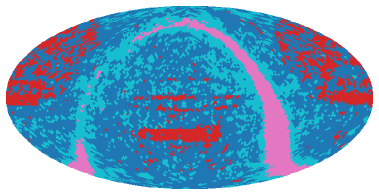
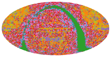
Figure 2: The masks that emerge when applying to GLADE the pattern recognition algorithm described in the text, with 4 masks (left) and 10 masks (right). The different colors, chosen as non-sequential for visual clarity, define the masks.

The choice $\Delta z=0.05$ provides relatively large bins in the radial directions. This allows us to have a sufficiently large volume ${\cal S}$, in the sense discussed above, even restricting to a rather narrow cone, as obtained with $\theta_{c}=5^{\circ}$. In this sense, cone completeness is a good quasi-local property from the angular point of view, but might imply too much coarse graining in the radial direction, especially considering that the completeness of GLADE drops relatively fast with redshift. A complementary option is to reduce the binning in the radial direction to about $\Delta z\lesssim 0.01$. This reduces the volume of the region ${\cal S}$, with the result that the true number of galaxies inside it might no longer be representative of the expected average value. To compensate, we attempt to include into one single region ${\cal S}$ all the areas in which the sky has been observed with similar telescope time and instrument characteristics, and in which the masking due to dust is also similar. Instead of increasing the cone opening angle, which would smooth out changes of these features with angle, that can be seen to be sharp transitions in Fig. 19 in app. A, we introduce a mask. It assigns each direction on the sky to one of a few regions, making the completeness at fixed redshift a piecewise constant function on the sphere. The mask is generated using a basic machine learning technique. We start by splitting the sky into a set of small cones, or rather HEALPix [97] pixels in practice, and then group similar pixels together by solving a clustering problem. The most relevant feature of the small cones for this purpose is the total number of galaxies within them. We found agglomerative clustering applied to this single feature to work sufficiently well. The number of clusters is chosen by hand, and we find that should not be less than about 4-5 for GLADE. The use of a single cluster reduces to the completeness defined over a $4\pi$ spherical shell with radial size between $z-\Delta z/2$ and $z+\Delta z/2$ (this is still more refined than the completeness used in [99, 31], which uses a $4\pi$ ball extending in redshift from zero to $z$), while two clusters can handle footprints of surveys like DES and GWENS, or exclude the galactic plane for GLADE. We find no evidence that more than 10 clusters are needed for the considered catalogs. An example of the masks that emerge by this procedure, when applied to the GLADE catalog, is shown in Fig. 2, with 4 masks (left panel) and 10 masks (right panel). Note that spatial proximity is not a feature we use for the clustering, but the masks are nevertheless mostly connected if there are only a few of them. This changes for larger mask number. Eventually, for increasing mask number, mask completeness converges toward cone completeness with small independent cones of the opening angle of a pixel of the HEALPix pixelization we choose. Using masks allows us to adapt the redshift bin size $\Delta z$ as follows. First, we define the depth of a mask as the redshift $z_{\rm depth}$ that contains $90\%$ of the galaxies in the mask. We expect the completeness to be a function decaying significantly on that scale. We then subdivide the mask into 30 bins from $z=0$ to $z=z_{\rm depth}$. Typically, in the densest cluster we get in this way bins of size $\Delta z=0.014$, while in the faintest regions (apart from the galactic plane), the bin size is about $\Delta z=0.008$. We then compute the completeness, according to eq. (3.49), for the regions ${\cal S}$ defined in this way. We finally apply a smoothing filter to the $30$ values of completeness obtained in each mask, to further restrict sensitivity to intrinsic fluctuations of the galaxy structure.

3.2.2 Homogeneous and multiplicative completion

In the previous section we have introduced two quasi-local notions of completeness. Once assessed the level of completeness of a region ${\cal S}$, i.e. ‘how many galaxies are missing’, we still have to specify how exactly to complete it, i.e. how to distribute these galaxies within ${\cal S}$. Indeed, whether we use cone completeness or mask completeness, eq. (3.47) is an integrated relation (with the choice of cone vs. mask completeness reflected in the choice of the integration region ${\cal S}$) and, to exploit the information contained in it, we must still make some assumption on how the missing galaxies are distributed within the region ${\cal S}$. Below, we examine two natural possibilities. In the following, for definiteness, we use the notation appropriate to cone completeness, with the region ${\cal S}$ denoted as ${\cal S}(z,\hat{\Omega};\Delta z,\Delta\Omega)$, but the considerations below are straightforwardly adapted to mask completeness, with an index $I$ labeling the region ${\cal S}_{I}$ corresponding to the $I$-th mask.

Homogeneous completion. The simplest hypothesis is to assume that, within the region ${\cal S}(z,\hat{\Omega};\Delta z,\Delta\Omega)$, $n_{\rm miss}(z^{\prime},\hat{\Omega}^{\prime})$ is distributed uniformly, i.e. has a value that depends only on the ‘central’ values of $z,\hat{\Omega}$ that enter in the definition of the region ${\cal S}(z,\hat{\Omega};\Delta z,\Delta\Omega)$, but not on the ‘microscopic’ variables $z^{\prime},\hat{\Omega}^{\prime}$ that are used to span that region. In that case, from eq. (3.47),

$$n_{\rm miss}(z,\hat{\Omega};\Delta z,\Delta\Omega) = \bar{n}_{\rm gal}-\frac{1}{V_{c}({\cal S})}\,\int_{\cal S}dV^{\prime}_{c}\,n_{\rm cat}(z^{\prime},\hat{\Omega}^{\prime})$$ (3.50)

$$= \bar{n}_{\rm gal}-\frac{N_{\rm cat}({\cal S})}{V_{c}({\cal S})}\,.$$

Note that the dependence of $n_{\rm miss}$ on $(z,\hat{\Omega};\Delta z,\Delta\Omega)$ enters through ${\cal S}$. In terms of $P_{\rm compl}({\cal S})$, defined in eq. (3.49),

$$n_{\rm miss}(z,\hat{\Omega};\Delta z,\Delta\Omega)=\bar{n}_{\rm gal}\,\left[1-P_{\rm compl}(z,\hat{\Omega};\Delta z,\Delta\Omega)\right]\,.$$ (3.51)

We will refer to this procedure as ‘homogeneous completion’. In the following, to make the notation lighter, we will not write explicitly the arguments $\Delta z,\Delta\Omega$. It is, however, always understood that quantities such as $n_{\rm miss}(z,\hat{\Omega})$ are coarse-grained quantities, whose definition requires the introduction of a binning defined by $\Delta z,\Delta\Omega$, in the simple case of the section of a cone, or, more generally, the introduction of a region ${\cal S}$.

For homogeneous completion, from eqs. (3.41) and (3.51) we find

$$p_{\rm miss}(z,\hat{\Omega};{\cal R}) = \frac{1}{N_{\rm miss}({\cal R})}\,\bar{n}_{\rm gal}\,\left[1-P_{\rm compl}(z,\hat{\Omega})\right]\frac{dV_{c}}{dzd\Omega}$$ (3.52)

$$= \frac{N_{\rm gal}({\cal R})}{N_{\rm miss}({\cal R})}\,\left[1-P_{\rm compl}(z,\hat{\Omega})\right]\frac{1}{V_{c}({\cal R})}\,\frac{dV_{c}}{dzd\Omega}\,,$$

where, in the second line, we used $\bar{n}_{\rm gal}=N_{\rm gal}({\cal R})/V_{c}({\cal R})$. From eq. (3.36) (with $w_{\alpha}=1$) we have $1-f_{\cal R}=N_{\rm miss}({\cal R})/N_{\rm gal}({\cal R})$, and therefore, from eq. (3.35), the prior $p_{0}(z,\hat{\Omega};{\cal R})$ in the case of homogeneous completion is given by

$$p^{\rm hom}_{0}(z,\hat{\Omega};{\cal R})=f_{\cal R}\,p_{\rm cat}(z,\hat{\Omega};{\cal R})+\left[1-P_{\rm compl}(z,\hat{\Omega})\right]\,\frac{1}{V_{c}({\cal R})}\,\frac{dV_{c}}{dzd\Omega}\,.$$ (3.53)

We next express $f_{\cal R}$ in terms of $P_{\rm compl}(z,\hat{\Omega})$, as follows. We first define

$$\bar{n}_{\rm cat}(z,\hat{\Omega})=\frac{N_{\rm cat}({\cal S})}{V_{c}({\cal S})}\,.$$ (3.54)

This is the average density of the galaxies present in the catalog, within the region ${\cal S}={\cal S}(z,\hat{\Omega};\Delta z,\Delta\Omega)$ (as before, we have not written explicitly the bin sizes $\Delta z,\Delta\Omega$ among the arguments of $\bar{n}_{\rm cat}$). Equation (3.49) can then be written as

$$P_{\rm compl}(z,\hat{\Omega})=\frac{\bar{n}_{\rm cat}(z,\hat{\Omega})}{\bar{n}_{\rm gal}}\,.$$ (3.55)

Integrating this equation over the whole region ${\cal R}$ used to define $f_{\cal R}$, and dividing by $V_{c}({\cal R})$, we get

$$\frac{1}{V_{c}({\cal R})}\,\int_{\cal R}dV^{\prime}_{c}\,P_{\rm compl}(z^{\prime},\hat{\Omega}^{\prime})=\frac{N_{\rm cat}({\cal R})}{N_{\rm gal}({\cal R})}\,.$$ (3.56)

The right-hand side is nothing but $f_{\cal R}$ (for the weights $w_{\alpha}=1$ that we are considering here), so

$$f_{\cal R}=\frac{1}{V_{c}({\cal R})}\,\int_{\cal R}dV^{\prime}_{c}\,P_{\rm compl}(z^{\prime},\hat{\Omega}^{\prime})\,.$$ (3.57)

Inserting this in eq. (3.53) we get the expression for the prior in the case of homogeneous completion, in the form

$$p^{\rm hom}_{0}(z,\hat{\Omega};{\cal R})=\frac{1}{V_{c}({\cal R})}\left\{\left[\int_{\cal R}dV^{\prime}_{c}\,P_{\rm compl}(z^{\prime},\hat{\Omega}^{\prime})\right]p_{\rm cat}(z,\hat{\Omega};{\cal R})+\left[1-P_{\rm compl}(z,\hat{\Omega})\right]\,\,\frac{dV_{c}}{dzd\Omega}\right\}\,.$$ (3.58)

For $P_{\rm compl}(z,\hat{\Omega})=1$ we recover $p_{0}(z,\hat{\Omega};{\cal R})=p_{\rm cat}(z,\hat{\Omega};{\cal R})$, as it should, while in the absence of a catalog, i.e. for $P_{\rm compl}(z,\hat{\Omega})=0$, we get back the prior uniform in comoving volume. The above equations agree with those given in [31], while providing, in our view, a more clear conceptual basis.

In eq. (3.58) it is convenient to extract the factors of $H_{0}$ that are implicit in $dV_{c}$ and $dV_{c}/dzd\Omega$. We write the Hubble parameter as

$$H(z)=H_{0}E(z)\,,$$ (3.59)

so, for instance, in a spatially flat cosmological model with matter density $\Omega_{M}$, radiation density $\Omega_{R}$ and dark energy density $\rho_{\rm DE}(z)$, we have $E(z)=[\Omega_{M}(1+z)^{3}+\Omega_{R}(1+z)^{4}+\rho_{\rm DE}(z)/\rho_{0}]^{1/2}$. Similarly, we write

$$d_{\rm com}(z)\equiv c\int_{0}^{z}\,\frac{d\tilde{z}}{H(\tilde{z})}=\frac{c}{H_{0}}\int_{0}^{z}\,\frac{d\tilde{z}}{E(\tilde{z})}\equiv\frac{c}{H_{0}}\,u(z)\,.$$ (3.60)

Then, from eq. (3.38),

$$\frac{dV_{c}}{dzd\Omega}=\left(\frac{c}{H_{0}}\right)^{3}\,\frac{u^{2}(z)}{E(z)}\equiv\left(\frac{c}{H_{0}}\right)^{3}\,j(z)\,.$$ (3.61)

We also define the dimensionless comoving volume ${\cal V}_{c}$ of the region ${\cal R}$ from

$$V_{c}({\cal R})=\left(\frac{c}{H_{0}}\right)^{3}\,{\cal V}_{c}({\cal R})\,.$$ (3.62)

Notice that $d{\cal V}_{c}=j(z)dzd\Omega$, i.e. $j(z)$ is the Jacobian of the transformation from the dimensionless volume element $d{\cal V}_{c}$ to $dzd\Omega$. We also introduce the angular average of the completeness,

$$P_{\rm compl}(z)\equiv\int\frac{d\Omega}{4\pi}\,P_{\rm compl}(z,\hat{\Omega})\,.$$ (3.63)

Then (assuming henceforth that the region ${\cal R}$ is a spherical region whose radius, in redshift space, is $z_{\cal R}$),

$$\int_{\cal R}dV^{\prime}_{c}\,P_{\rm compl}(z^{\prime},\hat{\Omega}^{\prime})=\left(\frac{c}{H_{0}}\right)^{3}\,4\pi\,\int_{0}^{z_{\cal R}}dz^{\prime}\,j(z^{\prime})P_{\rm compl}(z^{\prime})\,,$$ (3.64)

and eq. (3.58) can be rewritten as

$$p^{\rm hom}_{0}(z,\hat{\Omega};{\cal R})=\frac{1}{{\cal V}_{c}(z_{\cal R})}\left\{\left[4\pi\int_{0}^{z_{\cal R}}dz^{\prime}\,j(z^{\prime})P_{\rm compl}(z^{\prime})\right]p_{\rm cat}(z,\hat{\Omega};{\cal R})+\left[1-P_{\rm compl}(z,\hat{\Omega})\right]\,j(z)\right\}\,.$$ (3.65)

where, for the spherical region ${\cal R}$, we have written ${\cal V}_{c}({\cal R})={\cal V}_{c}(z_{\cal R})$, and

$${\cal V}_{c}(z_{\cal R})=4\pi\int_{0}^{z_{\cal R}}dz\,j(z)\,.$$ (3.66)

We finally observe that (when using luminosity weighting, see below), in the local Universe, $P_{\rm compl}(z,\hat{\Omega})$ can be larger than one because of actual over-densities, see in particular Fig. 23 in app. A, and similarly it can be below one just because of local under-densities. For each direction $\hat{\Omega}$, we will therefore perform the completion only for $z>z_{*}(\hat{\Omega})$, where $z_{*}(\hat{\Omega})$ is the largest value of $z$ for which $P_{\rm compl}(z,\hat{\Omega})=1$. In other words, for $z<z_{*}(\hat{\Omega})$ the difference of $P_{\rm compl}(z,\hat{\Omega})$ with respect to 1 will be attributed to actual over-densities and under-densities, while for $z>z_{*}(\hat{\Omega})$ we attribute them to the lack of completeness. In particular this means that, in the regions where $P_{\rm compl}(z,\hat{\Omega})>1$, we set $n_{\rm miss}({\bf x})=0$, rather than giving it a meaningless negative value, as would follow from a blind use of eq. (3.51). So, for $z<z_{*}$, we simply set $p_{0}(z,\hat{\Omega};{\cal R})=p_{\rm cat}(z,\hat{\Omega};{\cal R})$, which is formally equivalent to setting $P_{\rm compl}(z,\hat{\Omega})=1$, while for $z\geq z_{*}(\hat{\Omega})$ we use the actual value of $P_{\rm compl}(z,\hat{\Omega})$ obtained from the catalog, and we use as prior $p_{0}(z,\hat{\Omega};{\cal R})$ the expression given in eq. (3.65).

Multiplicative completion. We now come back to the assumption that the missing galaxies are uniformly distributed within ${\cal S}$. This is not the only natural possibility. If, for instance, within ${\cal S}$ there are clusters, filaments and voids, and the galaxy surveys have explored this volume uniformly, it could be more natural to assume that the galaxies that have been missed reside preferentially near high-density regions rather than, say, in the middle of a void. In its most extreme form, this amounts to assuming that $n_{\rm miss}(z,\hat{\Omega})$ is proportional to $n_{\rm cat}(z,\hat{\Omega})$, i.e.

$$n_{\rm miss}(z^{\prime},\hat{\Omega}^{\prime})=b({\cal S})\,n_{\rm cat}(z^{\prime},\hat{\Omega}^{\prime})\,,$$ (3.67)

where $z^{\prime},\hat{\Omega}^{\prime}$ are the ‘microscopic’ integration variables within ${\cal S}$ that appears in eq. (3.47) and $b({\cal S})$ is a multiplicative ‘bias factor’ that depends on the region ${\cal S}$, i.e. on the average redshift and direction of the region. This factor is then determined from eq. (3.47), which gives

$$1+b({\cal S})=\frac{\bar{n}_{\rm gal}V_{c}({\cal S})}{N_{\rm cat}({\cal S})}=\frac{1}{P_{\rm compl}({\cal S})}\,.$$ (3.68)

We will refer to eq. (3.67) as the ‘multiplicative’ completion. Multiplicative completion can be seen as a quantitative formulation of the idea [23, 28] that, to perform the correlation of GW events with galaxy catalogs, it is not necessary to have a complete catalog, but it is enough to have a catalog that reproduces the clustering structure of the galaxies. An intermediate option, which might be the best justified physically, could be to distribute the missing galaxies with respect to the observed ones, according to the correlation length of the spatial distribution of the observed galaxies. In this work, however, we will limit ourselves to homogeneous and multiplicative completions.

Inserting eq. (3.67) into eqs. (3.41) and (3.35) we get, for the prior $p_{0}(z,\hat{\Omega};{\cal R})$ in the case of multiplicative completion,

$$p^{\rm multi}_{0}(z,\hat{\Omega};{\cal R})=\frac{N_{\rm cat}({\cal R})}{N_{\rm gal}({\cal R})}\,[1+b(z)]p_{\rm cat}(z,\hat{\Omega};{\cal R})\,.$$ (3.69)

Using eqs. (3.56) and (3.68), we finally get

$$p^{\rm multi}_{0}(z,\hat{\Omega};{\cal R})=\frac{1}{V_{c}({\cal R})}\,\left[\int_{\cal R}dV^{\prime}_{c}\,P_{\rm compl}(z^{\prime},\hat{\Omega}^{\prime})\right]\,\frac{1}{P_{\rm compl}(z,\hat{\Omega})}p_{\rm cat}(z,\hat{\Omega};{\cal R})\,.$$ (3.70)

Observe that eq. (3.70) is singular at the points $(z,\hat{\Omega})$ where $P_{\rm compl}(z,\hat{\Omega})=0$ since, there, both the numerator $p_{\rm cat}(z,\hat{\Omega};{\cal R})$ and the denominator $P_{\rm compl}(z,\hat{\Omega})$ vanish. In fact, multiplicative completion is only meaningful in regions where $P_{\rm compl}(z,\hat{\Omega})$ is above a minimum value, otherwise one would unreasonably amplify the effect of random detections of galaxies in regions that have been very under-covered by the surveys. For instance, it would not be meaningful to apply it to regions such as those obscured by the galactic plane, where the distribution of the relatively few galaxies observed might reflect, for instance, the existence of directions with less absorption in our Galaxy, such as the Baade window, and has nothing to do with the actual distribution of galaxies. In contrast, homogeneous completion provides a neutral, uninformative prior that can be applied even in regions of low completeness (of course, in practice, when the completeness is too low the correlation of the GW events with the galaxy catalog will anyhow become uninformative). When using multiplicative completion, we will therefore interpolate it with homogeneous completion, depending on the completeness of the region. A simple way to do so is to use, as a prior,

$$p^{\rm multi/hom}_{0}(z,\hat{\Omega};{\cal R}) \equiv \theta\left[P_{\rm compl}(z,\hat{\Omega})-P_{c}^{\rm min}\right]\,p^{\rm multi}_{0}(z,\hat{\Omega};{\cal R})$$ (3.71)

$$+\theta\left[P_{c}^{\rm min}-P_{\rm compl}(z,\hat{\Omega})\right]\,p^{\rm hom}_{0}(z,\hat{\Omega};{\cal R})\,,$$

where $\theta$ is the Heaviside theta function, and $P_{c}^{\rm min}$ is a threshold on the completeness, so that regions with $P_{\rm compl}(z,\hat{\Omega})>P_{c}^{\rm min}$ are completed multiplicatively, while in regions with $P_{\rm compl}(z,\hat{\Omega})<P_{c}^{\rm min}$ we apply homogeneous completion.

3.2.3 Completion with luminosity weighting

We can proceed similarly when the weights $w_{\alpha}$ are equal to the B- or K-band luminosity. The computation is the same as before, with the number of all galaxies per comoving volume, $n_{\rm gal}({\bf x})$, replaced by the luminosity per comoving volume of all galaxies, that we denote by $l_{\rm gal}({\bf x})$; $n_{\rm cat}({\bf x})$ is replaced by the luminosity per comoving volume of the galaxies in the catalog, $l_{\rm cat}({\bf x})$, and $n_{\rm miss}({\bf x})$ is replaced by the luminosity per comoving volume of the missed galaxies, $l_{\rm miss}({\bf x})$, all restricted to the desired band (and, possibly, with a lower cut on the luminosity of individual galaxies, see below). For all these quantities, we define $L({\cal R})=\int_{\cal R}d^{3}x\,l({\bf x})$. Then eqs. (3.39)–(3.41) are replaced by

$$p_{0}(z,\hat{\Omega};{\cal R}) = \frac{l_{\rm gal}({\bf x})}{L_{\rm gal}({\cal R})}\,\frac{dV_{c}}{dzd\Omega}\,,$$ (3.72)

$$p_{\rm cat}(z,\hat{\Omega};{\cal R}) = \frac{l_{\rm cat}({\bf x})}{L_{\rm cat}({\cal R})}\,\frac{dV_{c}}{dzd\Omega}\,,$$ (3.73)

$$p_{\rm miss}(z,\hat{\Omega};{\cal R}) = \frac{l_{\rm miss}({\bf x})}{L_{\rm miss}({\cal R})}\,\frac{dV_{c}}{dzd\Omega}\,.$$ (3.74)

The condition (3.47) is replaced by

$$\frac{1}{V_{c}({\cal S})}\,\int_{\cal S}dV^{\prime}_{c}\left[l_{\rm cat}(z^{\prime},\hat{\Omega}^{\prime})+l_{\rm miss}(z^{\prime},\hat{\Omega}^{\prime})\right]=\bar{l}_{\rm gal}\,,$$ (3.75)

where $\bar{l}_{\rm gal}$ is the average luminosity per comoving volume of a complete sample. This is obtained assuming that the luminosity of a complete sample follows the Schechter luminosity function,

$$\Phi(L)dL=\phi^{*}\,\left(\frac{L}{L^{*}}\right)^{\alpha}\,e^{-L/L^{*}}\,\frac{dL}{L^{*}}\,,$$ (3.76)

where $\phi^{*}$, $\alpha$ and $L^{*}$ are the Schechter parameters in the corresponding band. We restrict to galaxies with luminosity above a given minimum value $L_{\rm cut}$. Then, the average luminosity density of a sample of galaxies with $L>L_{\rm cut}$ is

$$\bar{l}_{\rm gal}(L_{\rm cut}) \equiv \int_{L_{\rm cut}}^{\infty}dL\,L\phi(L)$$ (3.77)

$$= \phi^{*}L^{*}\int_{L_{\rm cut}/L^{*}}^{\infty}dx\,x^{\alpha+1}e^{-x}$$

$$= \phi^{*}L^{*}\Gamma(\alpha+2,L_{\rm cut}/L^{*})\,,$$

where $\Gamma(\alpha,x)$ is the incomplete Gamma function. We will discuss in app. A the choice of Schechter parameters in the B and K bands, and the quality of the fit to the Schechter function of the galaxies in GLADE. The best choice of $L_{\rm cut}$ is determined by a compromise between the fact that, increasing this cut, we have less galaxies overall, and the fact that the remaining sample is more and more complete. As we discuss in app. A, for GLADE a good compromise is provided by $L_{\rm cut}=0.6L^{*}$ (both in B-band and in K-band), and we will henceforth use this as a default choice.

The definition (3.49) is then generalized to

$$P_{\rm compl}({\cal S};L_{\rm cut})\equiv\frac{L_{\rm cat}({\cal S};L_{\rm cut})}{\bar{l}_{\rm gal}(L_{\rm cut})V_{c}({\cal S})}\,,$$ (3.78)

where $L_{\rm cat}({\cal S};L_{\rm cut})$ is the total luminosity of the galaxy in the catalog, in the region ${\cal S}$, and with luminosity above $L_{\rm cut}$, and the notation stresses also the dependence of the various quantities on the chosen lower cutoff on the luminosity. Using cone completeness, the region ${\cal S}$ is written more explicitly as ${\cal S}(z,\hat{\Omega};\Delta z,\Delta\Omega;L_{\rm cut})$, and, correspondingly, $P_{\rm compl}({\cal S};L_{\rm cut})$ can be written as $P_{\rm compl}(z,\hat{\Omega};\Delta z,\Delta\Omega;L_{\rm cut})$. However, again, to keep the notation lighter, we will often simply write it as $P_{\rm compl}(z,\hat{\Omega})$; for mask completeness we use again the notation ${\cal S}_{I}$.

In terms of these variables, the computation of $p_{0}(z,\hat{\Omega};{\cal R})$ is identical to that performed for $w_{\alpha}=1$. So, in the case of isotropic completion, we get again eq. (3.65), while, assuming $l_{\rm miss}(z^{\prime},\hat{\Omega}^{\prime})=b({\cal S})\,l_{\rm cat}(z^{\prime},\hat{\Omega}^{\prime})$, we get again eq. (3.70), where, in both cases, $p_{\rm cat}(z,\hat{\Omega};{\cal R})$ now includes the weights $w_{\alpha}$ for the corresponding band, see eq. (3.33), and $P_{\rm compl}(z)$ is now given by eq. (3.78). Again, in the case of multiplicative completion, we will then interpolate it with homogeneous completion as in eq. (3.71).

Observe that the assignment of absolute luminosities to galaxies assumes a cosmology, in particular a value of $H_{0}$. However, changing $H_{0}$ only produces an overall multiplicative shift of the weights $w_{\alpha}$, which cancels among the numerators and denominators in eqs. (3.31), (3.33) and (3.34), and therefore does not affect the corresponding priors. There are also possible systematics in assuming a fixed luminosity function, since the latter could have a redshift-dependent evolution. Nevertheless, the error that this assumption may introduce is negligible at the current level of precision.

3.3 The normalization factors $\beta(H_{0})$ and $\beta(\Xi_{0})$

We now turn to the normalization factor, treating in parallel the cases $\lambda^{\prime}=\{H_{0}\}$ and $\lambda^{\prime}=\{\Xi_{0}\}$. We use eqs. (3.23) and (3.24), that we rewrite, respectively, as

$$\beta(H_{0})=\int_{0}^{z_{\cal R}}dz\int d\Omega\,P_{\rm det}[d_{L}(z,H_{0}),\hat{\Omega}]\,p_{0}(z,\hat{\Omega})\,,$$ (3.79)

and

$$\beta(\Xi_{0})=\int_{0}^{z_{\cal R}}dz\int d\Omega\,P_{\rm det}[d_{L}^{\,\rm gw}(z,\Xi_{0}),\hat{\Omega}]\,p_{0}(z,\hat{\Omega})\,,$$ (3.80)

where we have used the factorization (3.25) and we defined a detection probability averaged over the $\theta^{\prime}$ parameters,

$$P_{\rm det}[d_{L}(z,H_{0}),\hat{\Omega}]=\int d\theta^{\prime}\,P_{\rm det}[d_{L}(z,H_{0}),\hat{\Omega},\theta^{\prime}]\tilde{p}_{0}(\theta^{\prime})\,,$$ (3.81)

and, respectively,

$$P_{\rm det}[d_{L}^{\,\rm gw}(z,\Xi_{0}),\hat{\Omega}]=\int d\theta^{\prime}\,P_{\rm det}[d_{L}^{\,\rm gw}(z,\Xi_{0}),\hat{\Omega},\theta^{\prime}]\tilde{p}_{0}(\theta^{\prime})\,.$$ (3.82)

As discussed in sect. 3.2, $p_{0}(z,\hat{\Omega})$ actually depends also on the region ${\cal R}$, which must be specified in order to define it. However, from the discussion in sect. 3.2 and App. B, it follows that the final result for the posterior of $H_{0}$ (or $\Xi_{0}$) will not depend on the choice of ${\cal R}$, as long as it contains the localization region of all the detectable GW events (in the whole range of priors considered for $H_{0}$ or $\Xi_{0}$). In eqs. (3.79) and (3.80), to keep the notation lighter, we have not written explicitly the argument ${\cal R}$ in $p_{0}(z,\hat{\Omega};{\cal R})$ and in $\beta(H_{0};{\cal R})$, $\beta(\Xi_{0};{\cal R})$. Note also that the integral over $dz$ in eqs. (3.79) and (3.80) extends up to the maximum redshift $z_{\cal R}$ of the region ${\cal R}$ which has been used to define $p_{0}(z,\hat{\Omega};{\cal R})$. Note that, in eq. (3.81), if among the parameters $\theta^{\prime}$ we include the source frame masses $m_{i}$, there is a further dependence on the redshift, that we have not written explicitly, entering from the fact that the detection probability depends on the detector frame masses $m_{i}^{(d)}=m_{i}(1+z)$, see also footnote 12 on page 12.

Before entering in the details of the computations, it is interesting to understand physically the meaning of the normalization factor $\beta(H_{0})$ [or, similarly, of $\beta(\Xi_{0})$]. Its role is to offset a dependence on $H_{0}$ in the numerator of eq. (3.17), which is of purely geometric nature, and that is present even when the GW events are completely uncorrelated to the galaxy distribution. Indeed, changing $H_{0}$ has the effect of changing the redshift of the GW event (whose position has been determined through a measurement of $d_{L}$) with respect to the positions of the galaxies in the catalog, that, in contrast, have been determined by a direct measurement of their redshift, independently of $H_{0}$. Thus, for instance, for a given measured value of $d_{L}$, increasing $H_{0}$ has the effect of increasing the redshift inferred for the GW event. Increasing the redshift, also the prior $p_{0}(z)$ increases; for instance, in a distribution of galaxies uniform in comoving volume, where $n_{\rm gal}(z,\hat{\Omega})$ is independent of $z$, $p_{0}(z)$ increases as $d_{\rm com}^{2}(z)/H(z)$, see eqs. (3.38) and (3.39), and therefore as $z^{2}$ at low $z$. As a result, the correlation between the GW probability $p({\cal D}^{i}_{\rm GW}|z,\hat{\Omega},H_{0})$ and the prior $p_{0}(z,\hat{\Omega})$ necessarily increases if we increase $H_{0}$, since we are moving the events (in redshift) toward a region where the prior is higher (and, conversely, the correlation decreases as we decrease $H_{0}$). This is a geometric effect that takes place even if the GW event is totally uncorrelated with the galaxy distribution: for instance, it would take place even if we would randomly generate fictitious GW events, or for sources, such as primordial BHs, that might not be correlated with the distribution of luminous matter. The role of the normalization factor $\beta(H_{0})$ is to compensate for such ‘trivial’ geometric effects. Note that this volume effect could give highly non-trivial information when it comes to comparing the overall observed rate of events with the theoretical predictions as a function of $H_{0}$ or $\Xi_{0}$. This will be discussed in sect. 3.4, where we will see that, unfortunately, current astrophysical uncertainties on the rate make it difficult to exploit this information.

In the following subsections we will discuss the computation of $\beta(H_{0})$ [or $\beta(\Xi_{0})$] with increasing levels of sophistication. In the simplest approximation, one assumes a homogeneous distribution of galaxies and a monochromatic population of sources (i.e., binaries all with the same source-frame masses). The corresponding computation, performed in [15], is reviewed in sect. 3.3.1. To go beyond this result, we first consider the effect of the approximation that the distribution of galaxies is uniform in comoving volume. In principle, once made a choice for the prior $p_{0}(z,\hat{\Omega};{\cal R})$, the same choice should be consistently used both in the numerator of eq. (3.17) and in the denominator [i.e. in $\beta(H_{0})$]. In the numerator of eq. (3.17) we certainly cannot use a uniform density of galaxies: the meaning of the whole procedure is precisely to correlate the localization of the GW event, expressed by $p({\cal D}^{i}_{\rm GW}|d_{L}(z,H_{0}),\hat{\Omega})$, with the inhomogeneities of the galaxy distribution (i.e. with the actual positions of galaxies) expressed by $p_{0}(z,\hat{\Omega})$, to see which values of $H_{0}$ (or of $\Xi_{0}$, for modified gravity) maximize this correlation. If we take a uniform distribution of galaxies in the numerator, there is nothing to correlate with. For the denominator, however, the approximation of uniform distribution is a meaningful first approximation, since the correlation only appears at the numerator. Still, it is necessary to quantify the effect of this approximation, especially in view of the sub-percent accuracy that is the final aim of studies of $H_{0}$. In sect. 3.3.2 we will see that the computation of sect. 3.3.1 admits a simple and elegant generalization when the prior is taken to be that given by the full expression (3.65) for homogeneous completion, or by (3.70) for multiplicative completion.

In sect. 3.3.3 we will then include the effect of a more realistic detection model, for a population of BBHs with a distribution of masses. To some extent, this can be done with a semi-analytic approach that is quite instructive, and that we will discuss in app. C. Eventually, however, we will see that, in order to obtain reliable results, it will be necessary to restrict to GW events that fall in regions of sufficiently high completeness of the catalog used. This introduces a further selection effect, that must be taken into account in the computation of $\beta(H_{0})$ or $\beta(\Xi_{0})$, and that can only be reliably included with a full Monte Carlo (MC) computation. Furthermore, while the semi-analytic method that we will present uses only the inspiral part of the waveform, the use of full inspiral-merger-ringdown waveforms is necessary for BBHs with a large total mass (which is the case in particular for many detections of the O3a run), since these have only few inspiral cycles in the detector bandwidth. Our MC, which includes both the selection effect due to completeness and full inspiral-merger-ringdown waveforms, is described in app. D, and our final results, discussed in sect. 4 only make use of the MC computation of $\beta(H_{0})$ and $\beta(\Xi_{0})$.

3.3.1 Computation of $\beta$ assuming a homogeneous galaxy distribution

The first computation of $\beta(H_{0})$ was performed in [15]. In that computation the prior $p_{0}(z,\hat{\Omega})$ that enters in $\beta(H_{0})$, see eq. (3.79), has been taken to be that obtained from a distribution of galaxies uniform in comoving volume, i.e.

$$p_{0}(z,\hat{\Omega};{\cal R})=p_{0}(z;{\cal R})=\frac{1}{V_{c}({\cal R})}\,\frac{dV_{c}}{dzd\Omega}\,,$$ (3.83)

where $dV_{c}/dzd\Omega$ is given in eq. (3.38). This is formally equivalent to setting $P_{\rm compl}(z,\hat{\Omega})=0$ in eq. (3.58). Using eqs. (3.61), (3.62) and (3.66), and taking as usual for ${\cal R}$ a sphere in redshift space with radius $z_{\cal R}$, we can rewrite eq. (3.83) more explicitly as

$$p_{0}(z;z_{\cal R})=\frac{j(z)}{4\pi\int_{0}^{z_{\cal R}}dz^{\prime}j(z^{\prime})}\,,$$ (3.84)

with $j(z)$ defined by eqs. (3.59)–(3.61). The computation performed in [15] is also restricted to a monochromatic population of sources, e.g. BNS with $(1.4+1.4)M_{\odot}$. In this case one can use a simplified model for detection,

$$P_{\rm det}(d_{L})\equiv\int d\Omega\,P_{\rm det}(d_{L},\hat{\Omega})=\theta\left(d_{\rm max}-d_{L}\right)\,,$$ (3.85)

where $\theta$ is the Heaviside theta function and $d_{\rm max}$ is the value of the luminosity distance (averaged over the solid angle and over the $\theta^{\prime}$ parameters, so in particular over the source inclination) to which the given monochromatic population of source could be detected, given the sensitivity of the detector network. Equivalently, in terms of redshift, we can write

$$P_{\rm det}(z;H_{0})=\theta\left[z_{\max}(H_{0};d_{\rm max})-z\right]\,,$$ (3.86)

where $z_{\max}(H_{0};d_{\rm max})$ is the solution of $d_{L}(z;H_{0})=d_{\rm max}$. With these assumptions, one finds [15]

$$\beta_{0}(H_{0};d_{\rm max}) = \int_{0}^{z_{\cal R}}dz\int d\Omega\,P_{\rm det}[d_{L}(z,H_{0}),\hat{\Omega}]\,p_{0}(z,\hat{\Omega})$$ (3.87)

$$= \frac{1}{V_{c}({\cal R})}\,\int_{0}^{z_{\cal R}}dz\int d\Omega\,\frac{dV_{c}}{dzd\Omega}\theta\left[z_{\max}(H_{0};d_{\rm max})-z\right]$$

$$= \frac{V_{c}[H_{0},z_{\max}(H_{0};d_{\rm max})]}{V_{c}(H_{0},z_{\cal R})}\,.$$

The notation $\beta_{0}(H_{0};d_{\rm max})$ in this expression stresses that, with this simplified detection model, $\beta(H_{0})$ inherits a dependence on the choice of $d_{\rm max}$, and we also added a suffix ‘zero’ to distinguish the result of this ‘zero-th’ order approximation from the more elaborate results that we will present below. In the above expression, $V_{c}(H_{0},z_{\max})$ is the comoving volume of a sphere reaching the redshift $z_{\max}$, and we have similarly written $V_{c}({\cal R})$ as $V_{c}(H_{0},z_{\cal R})$. The notation $V_{c}[H_{0},z_{\max}(H_{0};d_{\rm max})]$ emphasizes that this quantity depends on $H_{0}$ both explicitly, through the overall $(c/H_{0})^{3}$ factor in eq. (3.62), and through $z_{\max}(H_{0};d_{\rm max})$. However, the explicit $(c/H_{0})^{3}$ factors cancel between $V_{c}[H_{0},z_{\max}(H_{0};d_{\rm max})]$ and $V_{c}(H_{0},z_{\cal R})$, so in the end the dependence on $H_{0}$ is only through $z_{\max}(H_{0};d_{\rm max})$. We can make this explicit by rewriting the result in terms of the dimensionless comoving volumes ${\cal V}_{c}$ defined in eq. (3.62),

$$\beta_{0}(H_{0};d_{\rm max}) = \frac{{\cal V}_{c}[z_{\max}(H_{0};d_{\rm max})]}{{\cal V}_{c}(z_{\cal R})}$$ (3.88)

$$= \frac{\int_{0}^{z_{\max}(H_{0};d_{\rm max})}dz\,j(z)}{\int_{0}^{z_{\cal R}}dz\,j(z)}\,.$$

For small values of $z_{\rm max}$, such that the Hubble law is valid, from eqs. (3.60) and (3.61) we have $u(z)\simeq z$ and $E(z)\simeq 1$ so $j(z)\simeq z^{2}$, and $z_{\rm max}(H_{0};d_{\rm max})\simeq H_{0}d_{\rm max}/c$; then eq. (3.88) gives

$$\beta_{0}(H_{0};d_{\rm max})\simeq\frac{z^{3}_{\rm max}(H_{0};d_{\rm max})}{3\int_{0}^{z_{\cal R}}dz\,j(z)}\simeq\frac{(H_{0}d_{\rm max}/c)^{3}}{3\int_{0}^{z_{\cal R}}dz\,j(z)}\,,$$ (3.89)

so $\beta_{0}(H_{0};d_{\rm max})\propto H_{0}^{3}$ [15]. However, the limit of small redshift is not appropriate in most situations, so the full expression (3.88) has rather been used in the literature.

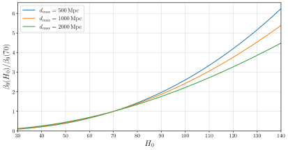
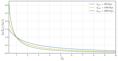
Figure 3: The functions $\beta_{0}(H_{0})$ (left panel) and $\beta_{0}(\Xi_{0})$ (right panel) computed as in eqs. (3.88) and (3.90), respectively. In order to show the results for different $d_{\rm max}$ on the same scale, we plot $\beta_{0}(H_{0})$ normalized to its value at $H_{0}=70~{}{\rm km}\,{\rm s}^{-1}\,{\rm Mpc}^{-1}$, and $\beta_{0}(\Xi_{0})$ normalized to its value at $\Xi_{0}=1$. In the left panel, as well as in all subsequent figures involving $H_{0}$, the units of the horizontal axis are ${\rm km}\,{\rm s}^{-1}\,{\rm Mpc}^{-1}$.

Note also that, in eq. (3.88), we made use of the fact that, by definition, $z_{\cal R}$ is chosen larger than $z_{\rm max}$ otherwise, formally, the integral over $z$ would give $\beta_{0}(H_{0};d_{\rm max})={\rm min}(1,{\cal V}_{c}[z_{\max}(H_{0};d_{\rm max})]/{\cal V}_{c}(z_{\cal R}))$. However, the condition $z_{\cal R}>z_{\rm max}$ is necessary for the consistency of the formalism, as we see from the derivation in app. B, and the apparent saturation of $\beta$ is just an artifact due to the fact that, if we take $z_{\cal R}<z_{\rm max}$, we miss some events in the count.

The corresponding result for $\beta_{0}(\Xi_{0};d_{\rm max})$ is trivially obtained replacing $z_{\max}(H_{0};d_{\rm max})$ by $z_{\max}(\Xi_{0};d_{\rm max})$, defined as the solution of $d_{L}^{\,\rm gw}(z;\Xi_{0})=d_{\rm max}$, so

$$\beta_{0}(\Xi_{0};d_{\rm max})=\frac{\int_{0}^{z_{\max}(\Xi_{0};d_{\rm max})}dz\,j(z)}{\int_{0}^{z_{\cal R}}dz\,j(z)}\,.$$ (3.90)

The result, for a few choices of $d_{\rm max}$, are shown in Fig. 3, for $\beta_{0}(H_{0})$ (left panel) and $\beta_{0}(\Xi_{0})$ (right panel).

3.3.2 Computation of $\beta$ including catalog completion

Homogeneous completion. We now generalize this computation to the full expression of the prior which includes the completion, still keeping for the moment the simplified detection model (3.86). We begin with homogeneous completion, so that the prior is given by eq. (3.65). Inserting eq. (3.65) into eq. (3.79), and using the detection model (3.86), we obtain [setting $z_{\cal R}$ sufficiently large, so that $z_{\rm max}(H_{0};d_{\rm max})<z_{\cal R}$ for the range of $H_{0}$ considered]

$$\beta^{\rm hom}(H_{0};d_{\rm max}) = \frac{\int_{0}^{z_{\cal R}}dz^{\prime}\,j(z^{\prime})P_{\rm compl}(z^{\prime})}{\int_{0}^{z_{\cal R}}dz^{\prime}\,j(z^{\prime})}\int_{0}^{z_{\rm max}(H_{0};d_{\rm max})}dz\int d\Omega\,p_{\rm cat}(z,\hat{\Omega};{\cal R})$$ (3.91)

$$+\frac{1}{\int_{0}^{z_{\cal R}}dz^{\prime}\,j(z^{\prime})}\,\int_{0}^{z_{\rm max}(H_{0};d_{\rm max})}dz\,j(z)\,\left[1-P_{\rm compl}(z)\right]\,,$$

where we also used eqs. (3.63) and (3.66). Inserting the expression (3.33) for $p_{\rm cat}(z,\hat{\Omega})$, we get our final result,

$$\beta^{\rm hom}(H_{0};d_{\rm max}) = \left(\frac{\int_{0}^{z_{\cal R}}dz^{\prime}\,j(z^{\prime})P_{\rm compl}(z^{\prime})}{\int_{0}^{z_{\cal R}}dz^{\prime}\,j(z^{\prime})}\right)\,\frac{\sum_{\alpha:z_{\alpha}<z_{\rm max}(H_{0};d_{\rm max})}w_{\alpha}}{\sum_{\alpha=1}^{N_{\rm cat}({\cal R})}w_{\alpha}}$$ (3.92)

$$+\frac{1}{\int_{0}^{z_{\cal R}}dz^{\prime}\,j(z^{\prime})}\,\int_{0}^{z_{\rm max}(H_{0};d_{\rm max})}dz\,j(z)\,\left[1-P_{\rm compl}(z)\right]\,,$$

where, in the first term, the sum in the numerator is restricted to the galaxies with redshift $z_{\alpha}<z_{\rm max}(H_{0};d_{\rm max})$, while that in the denominator is over all the galaxies of the catalog in the region ${\cal R}$. If one rather uses eq. (3.29) instead of the Dirac delta’s, we remain with a convolution in redshift involving the likelihoods for the $z_{\alpha}$.

In the limit $P_{\rm compl}(z,\hat{\Omega})\rightarrow 0$, we recover eq. (3.88). In the opposite limit $P_{\rm compl}(z,\hat{\Omega})\rightarrow 1$ we get

$$\beta^{\rm hom}(H_{0};d_{\rm max})=\frac{\sum_{\alpha:z_{\alpha}<z_{\rm max}(H_{0};d_{\rm max})}w_{\alpha}}{\sum_{\alpha=1}^{N_{\rm cat}({\cal R})}w_{\alpha}}\,.$$ (3.93)

For $w_{\alpha}=1$, this reduces to

$$\beta^{\rm hom}(H_{0};d_{\rm max})=\frac{N_{\rm cat}(z<z_{\rm max})}{N_{\rm cat}(z<z_{\cal R})}\,,$$ (3.94)

where $N_{\rm cat}(z<z_{\rm max})$ is the number of galaxies in the catalog with $z<z_{\rm max}(H_{0})$, and $N_{\rm cat}(z<z_{\cal R})$ is the number of galaxies in the catalog with $z<z_{\cal R}$. If the galaxies in the catalog are distributed uniformly in comoving volume, this is again the same as the ratio $V_{c}[z_{\max}(H_{0})]/V_{c}(z_{\cal R})$, so we expect that eq. (3.88) should be a reasonable zero-th order approximation.

It is straightforward to repeat these computations for $\beta(\Xi_{0})$. The only modification is that $z_{\rm max}(H_{0};d_{\rm max})$ is replaced by $z_{\rm max}(\Xi_{0};d_{\rm max})$, which is defined as the solution of

$$d_{L}^{\,\rm gw}(z_{\rm max},\Xi_{0})=d_{\rm max}\,.$$ (3.95)

Therefore

$$\beta^{\rm hom}(\Xi_{0};d_{\rm max}) = \left(\frac{\int_{0}^{z_{\cal R}}dz^{\prime}\,j(z^{\prime})P_{\rm compl}(z^{\prime})}{\int_{0}^{z_{\cal R}}dz^{\prime}\,j(z^{\prime})}\right)\,\frac{\sum_{\alpha:z_{\alpha}<z_{\rm max}(\Xi_{0};d_{\rm max})}w_{\alpha}}{\sum_{\alpha=1}^{N_{\rm cat}({\cal R})}w_{\alpha}}$$ (3.96)

$$+\frac{1}{\int_{0}^{z_{\cal R}}dz^{\prime}\,j(z^{\prime})}\,\int_{0}^{z_{\rm max}(\Xi_{0};d_{\rm max})}dz\,j(z)\,\left[1-P_{\rm compl}(z)\right]\,.$$

Multiplicative completion. We now consider multiplicative completion (at first without interpolation with homogeneous completion), so that the prior is given by eq. (3.70). Repeating the same steps as above, eq. (3.92) is replaced by

$$\beta^{\rm multi}(H_{0};d_{\rm max})=\left(\frac{\int_{0}^{z_{\cal R}}dz^{\prime}\,j(z^{\prime})P_{\rm compl}(z^{\prime})}{\int_{0}^{z_{\cal R}}dz^{\prime}\,j(z^{\prime})}\right)\,\frac{\sum_{\alpha:z_{\alpha}<z_{\rm max}(H_{0};d_{\rm max})}w_{\alpha}/P_{\alpha}}{\sum_{\alpha=1}^{N_{\rm cat}({\cal R})}w_{\alpha}}\,.$$ (3.97)

where we have defined

$$P_{\alpha}\equiv P_{\rm compl}(z_{\alpha},\hat{\Omega}_{\alpha})\,.$$ (3.98)

The factor $1/P_{\alpha}$ in eq. (3.97) reflects the fact that, within multiplicative completion, in regions where the completeness is smaller than one each observed galaxy is assumed to be representative of many more galaxies, and is therefore weighted with an extra factor $1/P_{\alpha}$. Once we interpolate between multiplicative and homogeneous completion, using eq. (3.71) as a prior, we get

$$\beta^{\rm multi/hom}(H_{0};d_{\rm max}) = \left(\frac{\int_{0}^{z_{\cal R}}dz^{\prime}\,j(z^{\prime})P_{\rm compl}(z^{\prime})}{\int_{0}^{z_{\cal R}}dz^{\prime}\,j(z^{\prime})}\right)\,$$

$$\times\frac{\sum_{\alpha:z_{\alpha}<z_{\rm max}(H_{0};d_{\rm max})}\left\{\theta[P_{\rm compl}(z_{\alpha},\hat{\Omega}_{\alpha})-P_{c}^{\rm min}]w_{\alpha}/P_{\alpha}+\theta[P_{c}^{\rm min}-P_{\rm compl}(z_{\alpha},\hat{\Omega}_{\alpha})]w_{\alpha}\right\}}{\sum_{\alpha=1}^{N_{\rm cat}({\cal R})}w_{\alpha}}$$

$$+\frac{1}{\int_{0}^{z_{\cal R}}dz^{\prime}\,j(z^{\prime})}\,\int_{0}^{z_{\rm max}(H_{0};d_{\rm max})}dz\,j(z)\,\int\frac{d\Omega}{4\pi}\,\theta[P_{c}^{\rm min}-P_{\rm compl}(z,\hat{\Omega})]\,\left[1-P_{\rm compl}(z,\Omega)\right]\,.$$

The corresponding expressions for $\beta(\Xi_{0};d_{\rm max})$ are obtained again replacing $z_{\rm max}(H_{0};d_{\rm max})$ by $z_{\rm max}(\Xi_{0};d_{\rm max})$.

3.3.3 Inclusion of the distribution of source parameters and more realistic detection model

The computation of $\beta(H_{0})$ and $\beta(\Xi_{0})$ discussed above still has a main limitation, particularly when applied to an ensemble of $N_{\rm obs}$ observed events, due to the simplified detection model (3.85). For an ensemble of events with different parameters, such as masses, inclination, etc., there is no notion of maximum detection distance. The distance to which an event can be detected depends strongly on its parameters, in particular on the masses of the components of the binary system, and on the inclination of the orbit.

The most direct way of including these effects is to perform a Monte Carlo (MC) evaluation of $\beta$ (the technical detail sof our MC are discussed in app. D) although one can get several insights also with a semi-analytic approximation, that we will discuss in app. C. Both for the semi-analytic approximation and for the MC evaluation, we consider BBHs with a distribution of component masses $\tilde{p}_{0}(m_{1},m_{2})$ (we use a tilde to distinguish it from the various other probability distributions that entered above). The formalism can be developed for an arbitrary choice of $\tilde{p}_{0}(m_{1},m_{2})$, but, for presenting the numerical results, we will use a broken power-law distribution, which is one of the models proposed in [6], where it is shown that it provides a good fit to the ensemble of BBHs observed in the O1,O2 and O3a LIGO/Virgo runs. This is given by

$$\tilde{p}_{0}(m_{1},m_{2})dm_{1}dm_{2}=\tilde{p}_{0}(m_{1})\tilde{p}_{0}(m_{2}|m_{1})dm_{1}dm_{2}\,,$$ (3.100)

where $m_{2}<m_{1}$. The function $\tilde{p}_{0}(m_{1})$ is chosen to follow a broken power law, $\tilde{p}_{0}(m_{1})\propto m_{1}^{-\gamma_{1}}$ for $m_{\rm min}<m_{1}<m_{\rm break}$ and $\tilde{p}_{0}(m_{1})\propto m_{1}^{-\gamma_{2}}$ for $m_{\rm break}<m_{1}<m_{\rm max}$, while the conditional distribution of the lighter mass, $\tilde{p}_{0}(m_{2}|m_{1})$, is taken to be proportional to $(m_{2}/m_{1})^{b_{q}}$, for some parameters $\gamma_{1},\gamma_{2},b_{q}$. The distribution is taken to vanish outside the interval $[m_{\rm min},m_{\rm max}]$. More precisely, for $\tilde{p}_{0}(m_{2}|m_{1})$ (writing explicitly its normalization factor, that depends on $m_{1}$) we have

$$\tilde{p}_{0}(m_{2}|m_{1})=\frac{1+b_{q}}{m_{1}}\,\frac{(m_{2}/m_{1})^{b_{q}}}{1-(m_{\rm min}/m_{1})^{1+b_{q}}}\,.$$ (3.101)

For $b_{q}=0$, corresponding to a conditional distribution flat in $m_{2}$, this reduces to $\tilde{p}_{0}(m_{2}|m_{1})=1/(m_{1}-m_{\rm min})$ [106]. Then

$$\tilde{p}_{0}(m_{1},m_{2})=A\,\frac{(m_{2}/m_{1})^{b_{q}}}{m_{1}[1-(m_{\rm min}/m_{1})^{1+b_{q}}]}\,\times\left\{\begin{array}[]{lc}(m_{1}/m_{\rm break})^{-\gamma_{1}}&\hskip 28.45274pt(m_{\rm min}<m_{1}<m_{\rm break})\\ (m_{1}/m_{\rm break})^{-\gamma_{2}}&\hskip 28.45274pt(m_{\rm break}<m_{1}<m_{\rm max})\end{array}\right.\,,$$ (3.102)

where $A$ is an overall normalization constant independent of $m_{1},m_{2}$, and we have enforced continuity at $m_{1}=m_{\rm break}$. The values of the various parameters that enter the distribution are determined by a fit to the masses of the observed BBHs and depend on several details such as, for instance, on whether GW190814, with its very low secondary mass, is considered a binary BH or not. The values obtained from the fit to the GWTC-2 data are

$$m_{\rm min}=2.2^{+0.27}_{-0.20}\,M_{\odot}\,,\qquad m_{\rm max}=86.16^{+12.37}_{-13.65}\,M_{\odot}\,,$$ (3.103)

$$\gamma_{1}=1.05^{+0.68}_{-1.08}\,,\qquad\gamma_{2}=5.17^{+3.22}_{-2.31}\,,\qquad b_{q}=0.28^{+1.28}_{-1.04}\,,$$ (3.104)

and

$$b_{\rm break}=0.41^{+0.16}_{-0.14}\,,$$ (3.105)

where $b_{\rm break}$ determines $m_{\rm break}$ from $m_{\rm break}=m_{\rm min}+b_{\rm break}(m_{\rm max}-m_{\rm min})$, so the mean value of $m_{\rm break}$ is $36.76\,M_{\odot}$. To have a quantitative idea of the dependence of the results on these choices, in sect. 4 we will vary the parameter $\gamma_{1}$, as well as the mass scales $m_{\rm break}$ and $m_{\rm max}$, first over the typical range of values which corresponds to their errors in the fit. It should be observed, however, that the fit to the mass function in ref. [105] is performed under the assumption of a fixed cosmology. Varying also the cosmology would broaden the allowed range of the parameters that enter in the mass function. We will therefore examine also the effect of larger variations of these parameters.

We first briefly summarize the results of the semi-analytic approximation, relegating the (rather long) technical details to App. C. For $\beta(H_{0})$, using homogeneous completion, we find

$$\beta^{\rm hom}(H_{0}) = \left(\frac{\int_{0}^{z_{\cal R}}dz^{\prime}\,j(z^{\prime})P_{\rm compl}(z^{\prime})}{\int_{0}^{z_{\cal R}}dz^{\prime}\,j(z^{\prime})}\right)\,\frac{\sum_{\alpha=1}^{N_{\rm cat}({\cal R})}w_{\alpha}B[d_{L}(z_{\alpha},H_{0})]}{\sum_{\alpha=1}^{N_{\rm cat}({\cal R})}w_{\alpha}}$$ (3.106)

$$+\frac{1}{\int_{0}^{z_{\cal R}}dz^{\prime}\,j(z^{\prime})}\,\int_{0}^{z_{\cal R}}dz\,j(z)\,\left[1-P_{\rm compl}(z)\right]\,B[d_{L}(z,H_{0})]\,,$$

while, for multiplicative completion,

$$\beta^{\rm multi}(H_{0})=\frac{\sum_{\alpha=1}^{N_{\rm cat}({\cal R})}w_{\alpha}B[d_{L}(z_{\alpha},H_{0})]/P_{\alpha}}{\sum_{\alpha=1}^{N_{\rm cat}({\cal R})}w_{\alpha}}\,.$$ (3.107)

The function $B[d_{L}(z,H_{0})]$, defined in eq. (C.22), is obtained from an integration over the inclination of the orbits (with a flat prior) and over the distribution of the component BH masses. Comparing with eqs. (3.92) and (3.97), we see that the function $B[d_{L}(z,H_{0})]$ plays the role of a smooth cutoff function, that replaces the theta function $\theta[z_{\rm max}(H_{0};d_{\rm max})-z]$.

A plot of the function $B(d_{L})$ is shown in the left panel of Fig. 4, using the BBH mass function (3.102) with the parameters set to the best fit values given in eqs. (3.103)–(3.105). In the right panel we show the result for a (source-frame) mass function appropriate to neutron stars in BNS, taken to be flat in the interval $[1-3]M_{\odot}$. The corresponding results for $\beta^{\rm hom}(H_{0})$, for the BBH and BNS mass function, are shown in Fig. 5. Similar results are obtained for $\beta(\Xi_{0})$, in which simply $d_{L}^{\,\rm gw}(z,\Xi_{0})$ replaces $d_{L}(z,H_{0})$ in the argument of $B[d]$, and are shown in the right panel of Fig. 5, again for BBHs and BNSs.

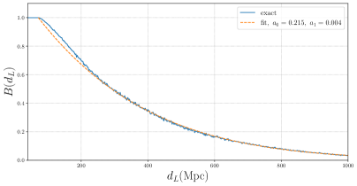
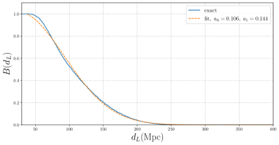
Figure 4: Left panel: The function $B[d_{L};z(d_{L},H_{0})]$ for BBHs, using the best fit values given in eqs. (3.103)–(3.105) in the BBH mass distribution (3.102) and the O2 strain sensitivity, and setting $H_{0}=70~{}{\rm km}\,{\rm s}^{-1}\,{\rm Mpc}^{-1}$. The blue solid curve is the numerical result and the dashed orange curve is the fit (C.29). Right panel: the function $B[d_{L};z(d_{L},H_{0})]$ for a BNS mass distribution, using a distribution for the source-frame masses flat in the range $[1-3]M_{\odot}$.

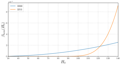
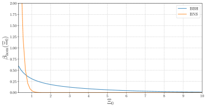
Figure 5: The functions $\beta_{\rm hom}(H_{0})$ (left) and $\beta_{\rm hom}(\Xi_{0})$ (right) for BBHs and for BNS, obtained using eq. (3.106), using the functions $B[d_{L};z(d_{L},H_{0})]$ shown in Fig. 4.

A further issue that deserves consideration is that, for a catalog such as GLADE, most of the events of the O2 and O3 LIGO/Virgo runs fall in regions of low or very low completeness; this is true in particular for all events at large redshift, given that, as we discuss in app. A, even with luminosity weighting and optimal choices of the cuts, GLADE becomes very incomplete beyond redshift $z\sim 0.2$. Events in region of very low completeness are in practice uninformative for our purpose of performing correlations between the GW events and the galaxy distribution and, if correctly treated, should give an essentially flat contribution to the posterior (at least after averaging over several such events). However, this flat contribution comes from a very delicate compensation of potentially large effects between the numerator and denominator of the posterior (3.11), and would require a very tight control over the function $\beta(H_{0})$ [or $\beta(\Xi_{0})$], including the precise BBH mass function, details of the detector sensitivities at time of detection, etc. A much more sound strategy, therefore, consists in simply excluding from the analysis the GW events that fall in regions of low completeness. This, however, introduces a selection effect that must be included also in the computation of $\beta$. In practice, this can only be done with a Monte Carlo (MC), which we perform to provide our final results.

Another element of the MC computation of $\beta(H_{0})$ [or of $\beta(\Xi_{0})$] is the choice of the waveform used for computing the SNR of a given event. The use of a waveform including only the inspiral part (that we have used in the semi-analytic technique, as described in app. C) could still be a reasonably good approximation for the O2 run. However, for the detections in the O3 run this is no longer the case, given the large total mass of many of the detected BBHs, that implies that they only have few inspiral cycles in the detector bandwidth, and a significant portion of the SNR comes from the merger (and possibly ringdown) phase. We therefore use full inspiral-merger-ringdown waveforms. In our MC, we use in particular the IMRPhenomXAS waveforms [107]. Note that this is still an approximation to the actual detection process, since it is based on a threshold on the SNR, as opposed to injecting mock signals into the actual detection pipelines.

3.4 Information from the overall rate

Finally, we consider the information that could be extracted from the total number of events detected in a given run, and from their redshift distribution. For definiteness, we use $\Xi_{0}$ in the discussion below since it can potentially give larger effects, but the equations apply to the case of $H_{0}$ with the replacement $\Xi_{0}\rightarrow H_{0}$.

Including the information on the rate, for an ensemble of $N_{\rm det}$ GW detections, the posterior (3.3) for $\Xi_{0}$ becomes [17]

$$p(\Xi_{0}|\{{\cal D}_{\rm GW}\})=p(N_{\rm det}|\Xi_{0})\,\,\frac{\pi(\Xi_{0})\prod_{i=1}^{N_{\rm det}}p({\cal D}^{i}_{\rm GW}|\Xi_{0})}{p(\{{\cal D}_{\rm GW}\})}\,,$$ (3.108)

where $p(N_{\rm det}|\Xi_{0})$ is the likelihood of detecting $N_{\rm det}$ events in the observation run, given $\Xi_{0}$. Since $\Xi_{0}$ effectively changes the horizon distance of the GW events, it can significantly affect the total number of detections. For instance, at $z=1$, for $\Xi_{0}=1.8$ we have $d_{L}^{\,\rm gw}/d_{L}^{\,\rm em}\simeq 1.6$, so the actual electromagnetic luminosity distance probed is smaller by a factor 1.6 compared to GR. For these redshifts, a reduction factor of about the same order takes place for the comoving distance, corresponding to a reduction by a factor $(1.6)^{3}\sim 4$ in the comoving volume explored. In principle, this is a large effect. However, to exploit it we need to have a comparably accurate estimate of the rate of BBH detections and of their distribution in redshift, in the absence of modified GW propagation. Unfortunately, this introduces large astrophysical uncertainties that, currently, seem to make difficult of obtaining convincing information on modified GW propagation from the the study of the overall number of detections and of their redshift distribution. This is apparent, for instance, from the clear discussion in [101]. The relevant quantity, to compute the number of detected events and their redshift distribution, is the differential mass-redshift distribution of BBH,

$$\frac{dN}{dm_{1}dm_{2}dz}=N_{\rm BBH}\,\tilde{p}_{0}(m_{1},m_{2},z)\,,$$ (3.109)

where $N_{\rm BBH}$ is the total number of BBHs across all masses and redshifts, and $\tilde{p}_{0}(m_{1},m_{2},z)$ is the (normalized) mass distribution, for which in sect. 3.3.3 we assumed an expression independent of redshift, given by eq. (3.102). Here, however, it is crucial to include also the redshift dependence, since this is partially degenerate with the effect of $\Xi_{0}$ on the rate. Note that, when computing the posterior $p({\cal D}^{i}_{\rm GW}|\Xi_{0})$ that expresses the GW-galaxy correlation, we are anyhow limited to small redshifts by the incompleteness of the galaxy catalog. For the overall rate we do not have this limitation, since it does not involve a correlation with galaxies, and indeed the effect become large only going to sufficiently large redshift. However, this also makes more important to understand the redshift dependence in $\tilde{p}_{0}(m_{1},m_{2},z)$.

Ref. [101] discusses several typical assumptions on $\tilde{p}_{0}(m_{1},m_{2},z)$, and their effect on the predictions. For instance, one in general starts from the simplifying assumption that the distribution factorizes, $\tilde{p}_{0}(m_{1},m_{2},z)=\tilde{p}_{0}(m_{1},m_{2})\tilde{p}_{0}(z)$, i.e. that the mass distribution of BBH does not evolve with $z$, an assumption that most probably breaks down at large redshift. One then proposes a parametrization for $\tilde{p}_{0}(m_{1},m_{2})$, involving some phenomenological and relatively poorly constrained parameters, such as eq. (3.102). For the redshift dependence, as we saw in eq. (3.42), for redshifts $z\,\raise 1.72218pt\hbox{$<$}\kern-8.00003pt\lower 2.6694pt\hbox{$\sim$}\,1$ a common parametrization is

$$\tilde{p}_{0}(z)\propto\frac{dV_{c}}{dz}\,(1+z)^{\lambda-1}\,,$$ (3.110)

where $V_{c}$ is comoving volume and $\lambda$ a free parameter, with $\lambda=0$ corresponding to a merger rate density uniform in comoving volume and source-frame time. However, as discussed below eq. (3.42), if the BBH merger rate follows the star formation rate (SFR), at low redshifts $z\,\raise 1.72218pt\hbox{$<$}\kern-8.00003pt\lower 2.6694pt\hbox{$\sim$}\,1$ one rather has $\lambda\sim 3$ while, convolving the SFR with a distribution of time delays between binary formation and merger can lead to estimates of $\lambda$ over a very broad range, from $\lambda\sim-10$ to $\lambda$ of order a few (see [101] for discussion and references).

With all these uncertainties on the mass distribution and redshift dependence, it is difficult to convincingly disentangle any extra redshift dependence on the BBH coalescence rate induced by modified GW propagation from the unknown redshift dependence of astrophysical origin (see fig. 2 of [101], where it is shown that the modification from a selected modified gravity model can be easily mimicked by changes in the astrophysical assumptions). The same limitations apply to the idea of exploiting the statistics of the signal-to-noise ratio from an ensemble of events, as attempted in refs. [108, 109, 110].

One could attempt to use the information on the rate only for events with $z\ll 1$, where one can hope to neglect the effect of source evolution. This could possibly be of use for the statistical measurement of $H_{0}$, but not for $\Xi_{0}$, because in the limit $z\ll 1$ also the effect of modified GW propagation disappears. Both modified GW propagation and astrophysical effects such as those parametrized in eq. (3.110) give corrections $1+{\cal O}(z)$ at low $z$, that, again, are very difficult to disentangle, at least with the current astrophysical uncertainties.

For this reason, in this work we will only consider the correlation with galaxy catalogs, and we will neglect the information potentially contained in the term $p(N_{\rm det}|\Xi_{0})$ in eq. (3.108). We will therefore set $p(N_{\rm det}|\Xi_{0})$ to a constant independent of $\Xi_{0}$ (and similarly for $H_{0}$). As shown in [31, 87], this is formally equivalent to marginalizing eq. (3.108) over the event rate $R$, assuming a prior $\pi(R)dR=dR/R$ i.e. a prior flat with respect to $\log R$, which is the typical prior that one use when one has no previous knowledge on a quantity, here $R$, that can vary over several orders of magnitudes.

3.5 Summary

We can now summarize the results of this long section as follows. From eq. (3.10), in the approximation in which we neglect the information on the total rate, the total likelihood for $H_{0}$ is

$$p(\{{\cal D}_{\rm GW}\}|H_{0})=\prod_{i=1}^{N_{\rm obs}}p(\{{\cal D}^{i}_{\rm GW}\}|H_{0})\,$$ (3.111)

where $p(\{{\cal D}^{i}_{\rm GW}\}|H_{0})$ is conveniently written as a ratio,

$$p(\{{\cal D}^{i}_{\rm GW}\}|H_{0})=\frac{n_{i}(H_{0})}{\beta(H_{0})}\,.$$ (3.112)

The expressions of the function $\beta(H_{0})$ and of the numerator $n_{i}(H_{0})$ depend on the prior $p_{0}(z,\hat{\Omega})$ and therefore on how we complete the catalog. We consider first the case in which the parameter $\lambda$ in eq. (3.45) is set to $\lambda=1$, so there is no redshift dependence in the prior induced by the merger rate. In this case, for homogeneous completion, inserting eqs. (3.33) and (3.65) into eq. (3.17) and using the likelihood (3.18) that depends on $z$ and $H_{0}$ [through $d_{L}(z,H_{0})$] and on $\hat{\Omega}$, we get

$$n_{i}(H_{0}) = \left[\frac{\int_{0}^{z_{R}}dz^{\prime}\,j(z^{\prime})P_{\rm compl}(z^{\prime})}{\int_{0}^{z_{R}}dz^{\prime}\,j(z^{\prime})}\right]\,$$

$$\times\left\{\frac{\sum_{\alpha=1}^{N_{\rm cat}({\cal R})}w_{\alpha}{\cal L}_{i}(z_{\alpha},\Omega_{\alpha};H_{0})}{\sum_{\alpha=1}^{N_{\rm cat}({\cal R})}w_{\alpha}}+\frac{\int_{0}^{z_{R}}dzj(z)\int d\Omega[1-P_{\rm compl}(z,\hat{\Omega})]\,\,{\cal L}_{i}(z,\hat{\Omega};H_{0})}{4\pi\int_{0}^{z_{R}}dz\,j(z)P_{\rm compl}(z)}\right\}\,,$$

where the jacobian $j(z)$ is defined in eq. (3.61); $P_{\rm compl}(z,\hat{\Omega})$ describes the completeness of the catalog, and has been defined in eqs. (3.49) or (3.55) for the case $w_{\alpha}=1$, and generalized in eq. (3.78) for the case of luminosity weighting. The structure in braces nicely shows how the catalog term is an average of the likelihood with respect to the weights $w_{\alpha}$, and the completion term is an average over the comoving volume, with the numerator weighted by $1-P_{\rm compl}(z,\hat{\Omega})$ and the denominator by $P_{\rm compl}(z)$. As we discussed below eq. (3.29) actually, rather than using a Dirac delta in redshift as in eq. (3.33), we use a full galaxy posterior. Then, the first term in braces ${\cal L}_{i}(z_{\alpha},\Omega_{\alpha};H_{0})$, which has been obtained by carrying out the integral over the redshift using a Dirac delta $\delta(z-z_{\alpha})$, is replaced by the full convolution in redshift.

We next include the effect of a generic parameter $\lambda$ in the merger rate. In this case, using eq. (3.45) [with $\tilde{p}_{0}(\theta^{\prime})=1$] we get

$$n_{i}(H_{0}) = c_{\lambda}\left[\frac{\int_{0}^{z_{R}}dz^{\prime}\,j(z^{\prime})P_{\rm compl}(z^{\prime})}{\int_{0}^{z_{R}}dz^{\prime}\,j(z^{\prime})}\right]\,\frac{\sum_{\alpha=1}^{N_{\rm cat}({\cal R})}w_{\alpha}(1+z_{\alpha})^{\lambda-1}{\cal L}_{i}(z_{\alpha},\Omega_{\alpha};H_{0})}{\sum_{\alpha=1}^{N_{\rm cat}({\cal R})}w_{\alpha}}$$ (3.114)

$$+c_{\lambda}\frac{\int_{0}^{z_{R}}dzj(z)(1+z)^{\lambda-1}\int d\Omega[1-P_{\rm compl}(z,\hat{\Omega})]\,\,{\cal L}_{i}(z,\hat{\Omega};H_{0})}{4\pi\int_{0}^{z_{R}}dz\,j(z)}\,.$$

The constant $c_{\lambda}$ is determined from eq. (3.46) and is independent of $H_{0}$, so it can be omitted. In any case, it is given by

$$c_{\lambda}^{-1} = \left[\frac{\int_{0}^{z_{R}}dz^{\prime}\,j(z^{\prime})P_{\rm compl}(z^{\prime})}{\int_{0}^{z_{R}}dz^{\prime}\,j(z^{\prime})}\right]\,\frac{\sum_{\alpha=1}^{N_{\rm cat}({\cal R})}w_{\alpha}(1+z_{\alpha})^{\lambda-1}}{\sum_{\alpha=1}^{N_{\rm cat}({\cal R})}w_{\alpha}}$$ (3.115)

$$+\frac{\int_{0}^{z_{R}}dzj(z)(1+z)^{\lambda-1}[1-P_{\rm compl}(z)]}{\int_{0}^{z_{R}}dz\,j(z)}\,.$$

Observe that, for a complete catalog, $P_{\rm compl}(z,\hat{\Omega})=1$, eqs. (3.114) and (3.115) reduce to

$$n_{i}(H_{0})=\frac{\sum_{\alpha=1}^{N_{\rm cat}({\cal R})}w_{\alpha}(1+z_{\alpha})^{\lambda-1}{\cal L}_{i}(z_{\alpha},\Omega_{\alpha};H_{0})}{\sum_{\alpha=1}^{N_{\rm cat}({\cal R})}w_{\alpha}(1+z_{\alpha})^{\lambda-1}}\,,$$ (3.116)

which amounts to using $w_{\alpha}(1+z_{\alpha})^{\lambda-1}$ as weights. Similarly, in the opposite limit $P_{\rm compl}(z,\hat{\Omega})=0$, eqs. (3.114) and (3.115) become

$$n_{i}(H_{0})=\frac{\int_{0}^{z_{R}}dzj(z)(1+z)^{\lambda-1}\,\,{\cal L}_{i}(z,\hat{\Omega};H_{0})}{\int_{0}^{z_{R}}dz\,j(z)(1+z)^{\lambda-1}}\,,$$ (3.117)

which corresponds to using a weight $j(z)(1+z)^{\lambda-1}$. However, in the presence of both the catalog term and the completion term, the result is more complicated, since the normalization constant involves both. We similarly compute the function $\beta(H_{0})$ by performing a Monte Carlo (MC) integration using eq. (3.45) as the prior.

Repeating the computation for purely multiplicative completion, we get

$$n_{i}(H_{0})=\frac{\sum_{\alpha}P_{\alpha}^{-1}w_{\alpha}(1+z_{\alpha})^{\lambda-1}{\cal L}_{i}(z_{\alpha},\Omega_{\alpha};H_{0})}{\sum_{\alpha}P_{\alpha}^{-1}w_{\alpha}(1+z_{\alpha})^{\lambda-1}}\,,$$ (3.118)

where $P_{\alpha}$ was defined in eq. (3.98). So, for pure multiplicative completion, each galaxy is weighted with a factor $P_{\alpha}^{-1}w_{\alpha}(1+z_{\alpha})^{\lambda-1}$. For the interpolation between multiplicative completion and homogeneous completion, in the case $\lambda=1$, inserting eqs. (3.33), (3.70) and (3.71) into eq. (3.17), and writing again the result in the form (3.112), we get

$$n_{i}(H_{0})=n_{i}^{(1)}(H_{0})+n_{i}^{(2)}(H_{0})\,,$$ (3.119)

where (apart from a normalization factor independent of $H_{0}$)

$$n_{i}^{(1)}(H_{0}) = \frac{1}{\sum_{\alpha=1}^{N_{\rm cat}({\cal R})}w_{\alpha}}$$

$$\times\sum_{\alpha=1}^{N_{\rm cat}({\cal R})}\left\{P_{\alpha}^{-1}w_{\alpha}(1+z_{\alpha})^{\lambda-1}\,\theta[P_{\rm compl}(z_{\alpha},\hat{\Omega}_{\alpha})-P_{c}^{\rm min}]\right.$$

$$\left.+w_{\alpha}(1+z_{\alpha})^{\lambda-1}\theta[P_{c}^{\rm min}-P_{\rm compl}(z_{\alpha},\hat{\Omega}_{\alpha})]\right\}{\cal L}_{i}(z_{\alpha},\Omega_{\alpha};H_{0})$$

and

$$n_{i}^{(2)}(H_{0})=\frac{\int_{0}^{z_{R}}dzj(z)\,(1+z)^{\lambda-1}\int d\Omega\,\theta[P_{c}^{\rm min}-P_{\rm compl}(z_{\alpha},\hat{\Omega}_{\alpha})]\,[1-P_{\rm compl}(z,\hat{\Omega})]\,\,{\cal L}_{i}(z,\hat{\Omega};H_{0})}{4\pi\int_{0}^{z_{R}}dz\,j(z)P_{\rm compl}(z)}\,,$$ (3.121)

where the theta functions are smoothed as in footnote 23 on page 23.

The denominator $\beta(H_{0})$ is computed through a MC evaluation, as discussed in sect. 3.3.3, using full inspiral-merger-ringdown waveforms. Details of our (publicly available) MC are given in app. D. The analysis is restricted to events that pass a cut in term of completeness (see footnote 32 on page 32 for details). The same cut is applied in the MC evaluation of $\beta(H_{0})$. The results for $\Xi_{0}$ are simply obtained replacing $H_{0}$ with $\Xi_{0}$ in the above expressions.

4 Results

We now present our results for the posteriors of $H_{0}$ and of $\Xi_{0}$, using the published data from the O1, O2 and O3a LIGO/Virgo runs. With current data, we cannot yet expect very stringent constraints. Our emphasis, however, will also be on the methodological aspects and on the dependence of the results on the various assumptions and approximations used, with the aim of understanding the systematic errors that, with the expected increase in the amount and quality of the GW data, will eventually become the limiting factor of the statistical method. In particular,

• we will compare the results obtained with different ways of quantifying the completeness of the catalog, i.e. mask vs. cone completeness, introduced in sect. 3.2.1. We will limit our main analysis to the GLADE catalog (see footnote 17 on page 17).

• For each of these two ways of quantifying the quasi-local completeness of the catalog, we will consider two different ways of distributing the missing galaxies, the homogeneous completion and the interpolation between multiplicative and homogeneous completion, introduced in sect. 3.2.2. For brevity, we will refer to the interpolation between multiplicative and homogeneous completion simply as ‘multiplicative completion’.

• As discussed at the end of sect. 3.3.3, GW events that fall in a region of low completeness should in principle give almost flat contributions to the posteriors. However, this comes from a delicate cancellation between the numerator and denominator of eq. (3.112) which, in practice, cannot be achieved unless one is able to compute the ‘exact’ expression for $\beta$, including the correct BBH mass function, the details of the detector sensitivities and their evolution during the run, etc. A better strategy is therefore to define the completeness of a GW event (relative to a given catalog) in terms of the completeness $P_{\rm comp}$ of the catalog in the region where it falls, and include only events whose completeness exceeds a threshold value $P_{\rm th}$. We will then have to account for this selection effect in the MC computation of the $\beta$ function. We will explore the effect of different choices for $P_{\rm th}$, in the range $0.1-0.7$.

• We will always use luminosity weighting, since, as discussed in app. A, for the GLADE catalog the weights $w_{\alpha}=1$ result in a level of completeness too low for the correlation with standard sirens. As discussed again in app. A, we adopt a lower cut on the luminosity $L_{\rm cut}=0.6L_{B}^{*}$ in B-band, and $L_{\rm cut}=0.6L_{K}^{*}$ in K-band. We will then compare the results obtained with B-band and with K-band luminosity weighting.

• We will study how the posterior of $H_{0}$ or $\Xi_{0}$ are affected by different choices for the values of the parameters that describe the astrophysical population. In particular, we will discuss the effect of changes in the parameters $m_{\rm break}$, $m_{\rm max}$ and $\gamma_{1}$ that characterize the BBH mass function (3.102), and of the parameter $\lambda$ that characterize the BBH rate (at low redshifts) according to eq. (3.42).

In order to avoid a proliferation of plots, in the main text we will only show the results for our ‘baseline’ set of choices, which is defined as follows: we use mask completeness (with 9 masks, but the results with, say, 5 masks, are very similar) to quantify the quasi-local completeness level of the catalog; we use multiplicative completion (more precisely, the interpolation between multiplicative and homogeneous completion) to distribute the missing galaxies; we use K-band luminosity weighting; and, finally, we set a rather high value of the completeness threshold, $P_{\rm th}=0.7$, for the selection of the GW events. In App. E we will justify these choices, and we will study how the results depend on them. As we will discuss there, mask completeness gives results consistent with cone completeness, and, similarly, homogeneous completion gives results consistent with multiplicative completions, within our (rather large) statistical uncertainty. In contrast, the choice of $P_{\rm th}$ is quite important, and, as we will discuss in App. E, we make the conservative choice of setting it to a rather high value, in order to minimize potential biases that could otherwise be induced by the GW events that fall in rather incomplete regions of the catalog. B-band is also consistent with K-band, but would require a higher completeness threshold to give similar results.

A consequence of the current limited statistics will be the dependence of the results on the range of prior chosen for $H_{0}$, and particularly on the upper limit. This is due to the fact that, for a given measured luminosity distance of the GW event, increasing $H_{0}$ corresponds to increasing the inferred redshift of the source and, as long as there are galaxies in the catalog at large $z$ (and as long as we complete the catalog, adding by hand ‘missing’ galaxies) we will always find a non-zero correlation. Therefore, the posterior on $H_{0}$ obtained from each individual GW event can extend to arbitrarily large values of $H_{0}$ (unless we use values of $H_{0}$ so high that the redshifts of the GW events are pushed into the dark epoch where no more galaxies are present, and we stop ‘completing’ the catalog), and is simply cut off by the choice of prior. As the mock data challenge in [17] shows, eventually, with a sufficiently large number of dark sirens, the total posterior on $H_{0}$ will take a well-behaved gaussian-like shape, with tails that become suppressed as we increase the number of events, effectively removing the dependence on the prior (see, in particular, Fig. 6 of [17]). However, with the current limited statistics of real data, we have to live with a dependence on the prior range chosen for $H_{0}$. In the following, we will use a flat prior in the range $[30,140]\,\,{\rm km}\,{\rm s}^{-1}\,{\rm Mpc}^{-1}$, similar to the prior $[20,140]\,\,{\rm km}\,{\rm s}^{-1}\,{\rm Mpc}^{-1}$ used in [32, 33]. When a posterior does not go to zero as we approach the upper limit of the prior range chosen, the notion of median value loses meaning, since the integral of the posterior distribution still gets significant extra contributions if we increase the upper limit of the prior range. In that cases, if the posterior shows a well defined peak, rather than the median value we quote the value at the maximum, which is independent of the prior range (as long as it includes the maximum), and the error that we quote corresponds to the $68\%$ highest density interval, i.e. the smallest interval which includes the maximum and contains $68\%$ of the area of the posterior; this quantity depends again on the prior range.

4.1 Hubble constant

4.1.1 Results using only dark sirens

We now present our results, using the BBH detections of the O1-O2 runs and of the O3a run. In Table 1 we list the O1-O2 BBH events, including some relevant data such as distance and masses, and the completeness at their nominal location (defined as in footnote 32), computed using cone completion (in B band and in K band), and using mask completion (again, in B band and K band). Observe that mask completeness gives higher values than cone completeness. This can be traced to the fact that cone completeness extends the region ${\cal S}$ toward larger redshifts compared to mask completeness, and increasing the redshift the catalog becomes less complete. In this sense, mask completeness seems a more faithful measure of the local completeness. In any case, we see that only few events have a high completeness. For instance, using mask completeness, both in B and K band there are 4 events that exceed a threshold $P_{\rm th}=0.5$, that reduce to 3 events if we raise the threshold to $P_{\rm th}=0.7$. We also observe that, for the majority of events, K band completeness is higher than B band completeness (the same happens for O3a data). We will discuss this further in app. E, and this will lead us to chose K-band in our baseline model. Observe also that events at comparable redshifts can have very different completeness level, according to our quasi-local notions of completeness (compare, for instance, GW170809 with GW170818). This shows the importance of using a quasi-local notion of completeness such as one of those that we have introduced, rather than a notion of completeness obtained from a $4\pi$ average.

name	$d_{L}$ (Mpc)	$z$	$m_{1}(M_{\odot})$	$m_{2}(M_{\odot})$	$P^{\rm cone}_{\rm comp,B}$	$P^{\rm cone}_{\rm comp,K}$	$P^{\rm mask}_{\rm comp,B}$	$P^{\rm mask}_{\rm comp,K}$
GW150914	440	0.09	35.6	30.6	0.75	1.00	1.00	1.00
GW151012	1080	0.21	23.2	13.6	0.00	0.05	0.04	0.07
GW151226	450	0.09	13.7	7.7	0.72	1.00	0.95	1.00
GW170104	990	0.20	30.8	20.0	0.10	0.41	0.27	0.41
GW170608	320	0.07	7.6	14.9	0.62	0.77	1.00	0.85
GW170729	2840	0.49	50.2	34.0	0.00	0.00	0.00	0.00
GW170809	1030	0.20	35.0	23.8	0.23	0.19	0.28	0.28
GW170814	600	0.12	30.6	25.2	0.36	0.69	0.52	0.57
GW170818	1060	0.21	35.4	26.7	0.01	0.06	0.03	0.08
GW170823	1940	0.35	39.5	29.0	0.00	0.00	0.00	0.00

Table 1: Values of luminosity distance (or GW luminosity distance, in the context of modified gravity), redshift (obtained from $d_{L}$ assuming $\Lambda$CDM with Planck cosmology) and source frame masses, for all BBH events detected in O1-O2 (from https://www.gw-openscience.org/eventapi/html/GWTC-1-confident/). In the last four columns we add the values of the completeness of GLADE at the nominal position of the event, computed using cone completeness (in B band and in K band), and mask completeness (again in B band and in K band).

We next consider the data from the O3a run [6]. The data release corresponds to 39 candidate GW events; given the threshold in the false alarm rate it is expected, statistically, that about $3$ of them will be false alarms. Despite this significantly larger number of events, compared to O2, we find that most of them fall into regions of very low completeness of GLADE, and are therefore not useful for correlation with this catalog. This is due to the fact that the increase in the number of detections comes from the increase of the reach of the detectors between O2 and O3, and so there are many more events at large redshift. However, these are precisely the events that are more likely to fall in regions where GLADE has low completeness. Table 2 lists all O3a events whose nominal position (defined as in footnote 32 on page 32) falls into a region with GLADE completeness higher than $0.1$, in at least one among B band and K band (restricting now, for definiteness, to mask completeness). We observe, from the value of the masses, that they all corresponds to BBH candidates, except for GW190426_152155, which has a component with mass $1.5M_{\odot}$, and it is rather a potential BH-NS binary. Its inclusion would therefore require a different computation of the beta function, with the mass function appropriate to BH-NS binaries, which is currently not really constrained. Furthermore, this is one of the three events in O3a (and the only one that makes it to Table 2) that, based on the false alarm rate, are more likely to be noise, rather than real GW events [6]. For these reasons, we will simply discard this event, and focus on the contribution from the BBH binaries in Table 2, which are all highly likely detections.

name	$d_{L}$ (Gpc)	$z$	$m_{1}(M_{\odot})$	$m_{2}(M_{\odot})$	$P^{\rm mask}_{\rm comp,B}$	$P^{\rm mask}_{\rm comp,K}$
GW190412	0.74	0.15	30.0	8.3	0.74	0.65
GW190426_152155	0.38	0.08	5.7	1.5	0.87	1.00
GW190527_092055	3.10	0.53	36.2	22.8	0.31	0.48
GW190630_185205	0.93	0.19	35.0	23.6	0.22	0.18
GW190707_093326	0.80	0.16	11.5	8.4	0.23	0.38
GW190708_232457	0.90	0.18	17.5	13.1	0.34	0.51
GW190814	0.24	0.05	23.2	2.59	1.00	1.00
GW190924_021846	0.57	0.12	8.8	5.0	0.99	1.00
GW190930_133541	0.78	0.16	12.3	7.8	0.20	0.24

Table 2: Median values of luminosity distance (or GW luminosity distance, in the context of modified gravity), redshift (obtained from $d_{L}$ assuming $\Lambda$CDM with Planck cosmology) and source frame masses, for the events in the O3a run (from [6]), restricting to the events whose mask completeness, either in B-band or in K-band (shown in the last two columns), is higher than $0.1$. As discussed in the text, we exclude GW190426_152155 (gray entry) from further analysis, since its masses do not correspond to a BBH and its false alarm probability is high.

In Fig. 6 we show the separate posterior for $H_{0}$ from the O1+O2 data and from the O3a data, and their combined posterior (the central lines corresponds to our reference value $\gamma_{1}=1.05$, while the shaded bands band give the effect of changing $\gamma_{1}$ within the range $\gamma_{1}=1.05^{+0.68}_{-1.08}$, as we will discuss in more detail below).

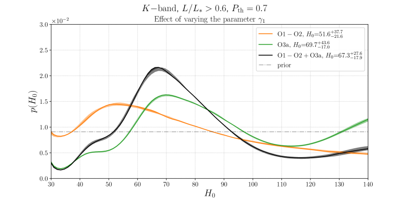
Figure 6: The separate posterior for $H_{0}$ from the O1+O2 data and from the O3a data, and their combined posterior, using mask completeness, multiplicative completion, K-band luminosity weighting, and a completeness threshold $P_{\rm th}=0.7$. The shaded bands give the effect of changing $\gamma_{1}$ within the range $\gamma_{1}=1.05^{+0.68}_{-1.08}$, with the central lines corresponding to our reference value $\gamma_{1}=1.05$.

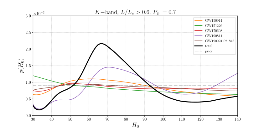
Figure 7: The separate contributions to the posteriors of $H_{0}$, from the individual events in O1+O2+O3a that pass the completeness threshold $P_{\rm th}=0.7$. The black line is the total posterior from O1+O2+O3a, already shown as the line inside the black band in Fig. 6.

Fig. 7 shows the separate contributions to the posterior of $H_{0}$, from the five events in O1+O2+O3a that pass the completeness threshold $P_{\rm th}=0.7$. We see that the single most important contribution comes from GW190814, followed by GW150914. Note, from Tables 1 and 2, that these two events have a completeness $P^{\rm mask}_{\rm comp}=1$. It is, however, interesting to remark that even if, individually, the other posteriors seem quite uninformative, still their combination produces a peak in the total posterior much more significant than that due to any single event. This nicely illustrates the power of the statistical method.

We observe that, with current statistics, the posterior for $H_{0}$ does not go to zero at the upper limit of the prior range considered (and in fact, for O3a, it even grows near the upper limit). Therefore, as discussed at the beginning of this section, the notion of median value loses meaning, since in this case it depends strongly on the prior range chosen. To condense the information contained in the posteriors shown in Fig. 6 into a single value of $H_{0}$ and a corresponding error, it is more meaningful to provide the value of the maximum of the posterior, with an error that corresponds to the $68\%$ highest density interval, i.e. the smallest interval which includes the maximum and contains $68\%$ of the area of the posterior. With this procedure, for the combined O1+O2+O3a data, we get

$$H_{0}=67.3^{+27.6}_{-17.9}\,\,\,\,{\rm km}\,{\rm s}^{-1}\,{\rm Mpc}^{-1}\,.$$ (4.1)

The maximum a posteriori values and the corresponding highest density intervals obtained separately from O1+O2 and from O3a are given in the inset of Fig. 6. Equation (4.1) corresponds to a measurement of $H_{0}$ at about $34\%$ accuracy from dark sirens only. This improves on the result $H_{0}=75^{+40}_{-32}\,\,{\rm km}\,{\rm s}^{-1}\,{\rm Mpc}^{-1}$ obtained in [32] by correlating the dark siren GW170814 with the DES galaxy catalog, and also on the result $H_{0}=66^{+55}_{-18}\,\,{\rm km}\,{\rm s}^{-1}\,{\rm Mpc}^{-1}$ obtained in [33] for the dark siren GW190814 (which is the event that gives the dominant contribution in our case), correlated with DES. Of course, the interest of these results is at a level of proof-of-principle of the statistical method, and much higher statistics will be needed to obtain an interesting accuracy.

We next investigate the dependence of the results on the astrophysical population parameters. We first vary the parameters $\gamma_{1}$, $m_{\rm break}$, $m_{\rm max}$ that enter in the broken power-law mass function (3.102) within the $1\sigma$ range found by the LVC fit, and we also vary the parameter $\lambda$ in the parametrization (3.110) of the merger rate, within the astrophysically plausible range $\lambda\in[0,3]$, which is also of the order of the range $\lambda=1.8^{+2.1}_{-2.2}$ ($90\%$ c.l.) obtained using the data from the GWTC-2 catalog [105], see the discussion below eq. (3.44). We present the results as an estimate of the corresponding systematic error. As already remarked, however, the mass distribution parameters, such as those given in eqs. (3.103) and (3.104), have been obtained from fits to the mass distribution, under the assumption of a fixed cosmology. The correct first-principle approach would be to turn this systematic error into a statistical error, by including the parameters that enter in the mass function into the set of parameters on which we wish to draw an inference, perform such a global inference, and finally present results for $H_{0}$ or $\Xi_{0}$ marginalized over the parameters that enter in the mass function. The same should be done for $\lambda$. Such a first-principle approach, however, would be numerically quite demanding. Given that anyhow the current dark sirens data do not yet allow us to get very stringent bounds on $H_{0}$ or $\Xi_{0}$, in this paper we limit ourselves to the simplest approach of fixing the parameters in the mass function to a reference value, and then vary this reference values within a plausible range, to obtain a first estimate of their effect, which, at this level, is treated as a systematic error. We begin by showing the results obtained varying the parameters in the mass function within the $1\sigma$ range found by the LVC fit, and $\lambda$ in the the range $\lambda\in[0,3]$. We will then show how the results change with more extreme values of these parameters, that might possibly emerge from changes in the underlying cosmology.

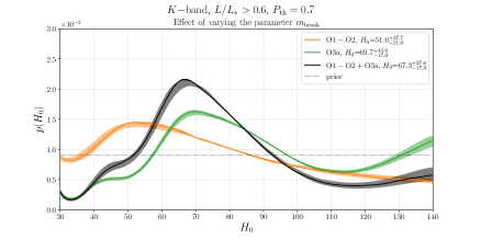
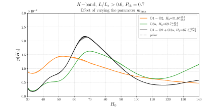
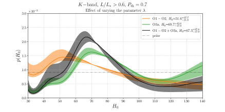
Figure 8: Upper row: the effect of changing $m_{\rm break}$ within the range $m_{\rm break}=36.76^{+11.37}_{-12.48}\,M_{\odot}$ (left panel) and the effect of changing $m_{\rm max}$ within the range $m_{\rm max}=86.16^{+12.37}_{-13.65}\,M_{\odot}$ (right panel). Lower panel: the effect of changing $\lambda$ in eq. (3.110) within the range $[0,3]$, with the central lines corresponding to our default value $\lambda=1$. We use mask completeness, multiplicative completion, K band, and a completeness threshold $P_{\rm th}=0.7$.

The effect of varying the parameter $\gamma_{1}$ within $1\sigma$ has already been shown in Fig. 6, where the shaded bands are obtained varying $\gamma_{1}$ within the range $\gamma_{1}=1.05^{+0.68}_{-1.08}$, which corresponds to its error in the fit to the observed BBH mass distribution [6]. In Fig. 8 the upper row (left panel) shows the effect of changing $m_{\rm break}$ within the range $m_{\rm break}=36.76^{+11.37}_{-12.48}\,M_{\odot}$, (corresponding to the $1\sigma$ variation of the LVC fit), with all other parameters of the mass function fixed at the reference values (3.103)–(3.105). The right panel shows the effect of changing $m_{\rm max}$ (with the other parameters fixed) in the interval $m_{\rm max}=86.16^{+12.37}_{-13.65}\,M_{\odot}$. We observe that changing $m_{\rm max}$ (at fixed $m_{\rm break}$) has only a minor effect. This can be understood from the fact that this only affects the tails of the mass distribution. The effects of changing $\gamma_{1}$ or $m_{\rm break}$ are more important, and somewhat comparable.

A much more important effect is obtained changing the parameter $\lambda$ that enters in the low-redshift limits of the BBH merger rate, eq. (3.42). The results are shown in the lower panel of Fig. 8, where the bands give the effect of changing $\lambda$ in eq. (3.110) within the astrophysically plausible range $[0,3]$, around our reference value $\lambda=1$. The effect becomes particularly large at small values of $H_{0}$, say $H_{0}<50\,\,\,{\rm km}\,{\rm s}^{-1}\,{\rm Mpc}^{-1}$. In principle, one could cut out this region with a narrower choice of prior range, given what we already know on $H_{0}$ from cosmological observation. Still, even in the most interesting range, say $H_{0}\in[60-80]\,\,\,{\rm km}\,{\rm s}^{-1}\,{\rm Mpc}^{-1}$, the effect of $\lambda$ on the shape of the posterior is quite significant, and appears to produce the dominant astrophysical uncertainty, at least among the astrophysical parameters that we have tested.

However, even if the shaded bands due to $\lambda$, in Fig. 8, are quite thick, the effect on the maximum a posteriori value and on the corresponding highest density intervals is not so large: for instance, for $\lambda=0$, we get $H_{0}=68.6^{+31.3}_{-18.1}$, while, for $\lambda=3$, we find $H_{0}=65.9^{+18.1}_{-21.6}$, to be compared with eq. (4.1) for $\lambda=1$. Of course, these results are all consistent, within their large statistical errors.

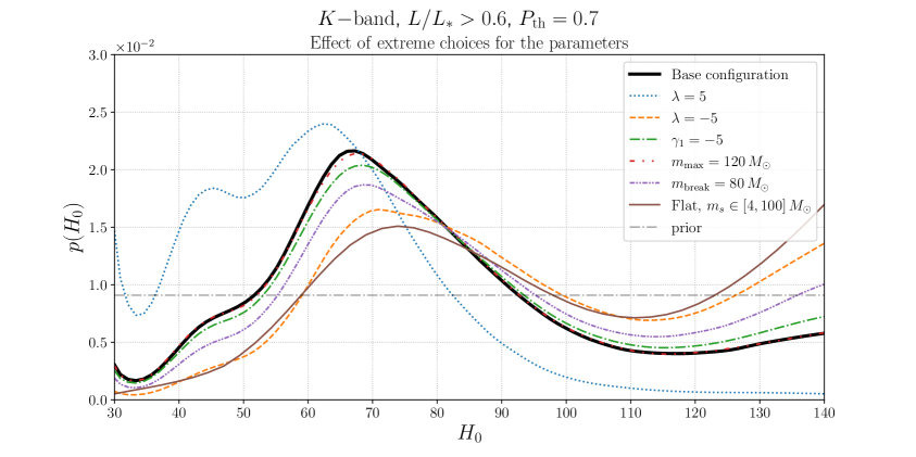
Figure 9: The baseline result compared with that obtained with some extreme choices for the values of the parameters in the mass function (3.102), as well as with a (source-frame) BBH mass distribution flat in the range $[4,100]M_{\odot}$.

In Fig. 9 we show how our baseline result changes with some more extreme choices for the values of these parameters. In particular (fixing each time all other parameters at our baseline configuration), we test the values $\lambda=5$ and $\lambda=-5$, as well as the value $m_{\rm max}=120M_{\odot}$, and the value $m_{\rm break}=80M_{\odot}$. We even consider, as an extreme case, a source-frame BBH mass distribution flat between $4M_{\odot}$ and $100M_{\odot}$. While, as expected, with such large changes the posterior for $H_{0}$ is appreciably modified, still we see that a clear peak always emerges, showing that the results are coming from the galaxy catalog and not from the assumed mass distribution.

In app. E we will study how the results presented here change with the completeness threshold, we will compare the results obtained for mask completeness with those obtained adopting cone completeness; for each of these two choices we will compare multiplicative with homogeneous completion, and we will compare K-band with B-band luminosity weighting.

4.1.2 Dark sirens combined with GW170817

Finally, it is interesting to combine the results obtained from dark sirens with the posterior for $H_{0}$ obtained from the BNS GW170817 and its electromagnetic counterpart. For GW170817, the likelihood (3.17) must be supplemented by the EM data about the position of the host galaxy NGC4993, and reads

$$p({\cal D}_{\rm GW},{\cal D}_{\rm EM}|H_{0})=\frac{1}{\beta(H_{0})}\int dzd\Omega d\theta^{\prime}\,p({\cal D}_{\rm EM}|z)p({\cal D}_{\rm GW}|d_{L}(z,H_{0}),\hat{\Omega},\theta^{\prime})\,p_{0}(z,\hat{\Omega},\theta^{\prime})\,,$$ (4.2)

where now $\beta(H_{0})$ is the normalization factor appropriate to BNS. The likelihood for the EM measurement is given by

$$p({\cal D}_{\rm EM}|z)=\mathcal{N}(z;z_{\rm EM},\sigma_{\rm EM})\times\delta\left(\hat{\Omega}-\hat{\Omega}_{\rm EM}\right)\,,$$ (4.3)

where $z_{\rm EM}$, $\sigma_{\rm EM}$ denote the mean and standard deviation of the redshift of the EM counterpart, and $\hat{\Omega}_{\rm EM}$ its angular position. For the mean and standard deviation of the redshift, it is important to take into account peculiar velocity corrections. The uncorrected value of the recession velocity of the host galaxy NGC4993 is $v=3327\pm 72\,\rm{km\;s^{-1}}$ [113, 18]. In principle, to fully take into account peculiar velocity corrections, one should add to eq. (4.2) a marginalisation over the peculiar velocity distribution. In Ref. [18] this is taken to be a gaussian with mean and standard deviation $v_{\rm p}=310\pm 150\,\rm{km\;s^{-1}}$. In this case the correction amounts to using in eq. (4.3) a gaussian with mean obtained by the recession velocity of NGC4993 corrected for the peculiar velocity, and standard deviation obtained by summing the errors in quadrature, which gives $v=3017\pm 166\,\rm{km\;s^{-1}}$. Ref. [114] uses a more refined estimate of the peculiar velocity PDF, resulting in $v_{\rm p}=373\pm 130\,\rm{km\;s^{-1}}$. The full PDF is non-gaussian, but in absence of its exact shape we will use a gaussian approximation with this mean and standard deviation. The resulting velocity of NGC4993 in this approximation is $v=2954\pm 149\,\rm{km\;s^{-1}}$. We shall use this value in the following, which corresponds to using $z_{\rm EM}=0.0098$, $\sigma_{\rm EM}=0.0004$ in eq. (4.2).

As for the prior $p_{0}(z,\hat{\Omega},\theta^{\prime})$, we take $\theta^{\prime}=\{m_{1},m_{2}\}$, where $m_{1},m_{2}$ are the source-frame masses, and we write the prior as $p_{0}(z,\hat{\Omega},\theta^{\prime})=\tilde{p}_{0}(z)\tilde{p}_{0}(m_{1},m_{2})$, as in sect. 3.4. Now, however, $\tilde{p}_{0}(m_{1},m_{2})$ is the distribution of (source-frame) NS masses in a BNS, and we take it to be flat between 1 and 3 solar masses. We choose $\tilde{p}_{0}(z)$ as in eq. (3.110), setting for definiteness $\lambda=1$. In any case, given the smallness of the redshift of GW170817, the choice of $\lambda$ is here irrelevant.

The term $p({\cal D}_{\rm GW}|d_{L}(z,H_{0}),\hat{\Omega},\theta^{\prime})$ in eq. (4.2) is the GW likelihood, marginalised over all variables except $d_{L}(z,H_{0}),\hat{\Omega}$, and $\theta^{\prime}=\{m_{1},m_{2}\}$. Using Bayes’ theorem and eq. (4.3), and integrating over $\hat{\Omega}$, we can rewrite eq. (4.2) as

$$p({\cal D}_{\rm GW},{\cal D}_{\rm EM}|H_{0}) = \frac{1}{\beta(H_{0})}\int dz\,\mathcal{N}(z;z_{\rm EM},\sigma_{\rm EM})\,\tilde{p}_{0}(z)$$ (4.4)

$$\times \int dm_{1}dm_{2}\,\frac{p(d_{L}(z,H_{0}),\hat{\Omega}_{\rm EM},m_{1},m_{2}|{\cal D}_{\rm GW})}{\pi(m_{1},m_{2})\pi(d_{L}(z,H_{0}))}\,\tilde{p}_{0}(m_{1},m_{2})\,.$$

where $\pi(m_{1},m_{2})$, $\pi(d_{L})$ are the prior used in the LVC analysis. The LVC provides posterior samples for GW170817 restricted to the sky location of the host galaxy [106], with a prior on luminosity distance $\pi(d_{L})\propto d_{L}^{2}$ and a flat prior in detector frame masses. Taking into account the $(1+z)$ factor between source frame and detector frame masses, the LVC prior is equivalent to $\pi(m_{1},m_{2})\propto(1+z)^{2}$, where $m_{1},m_{2}$ are the source-frame masses. To get the likelihood, we must divide the posteriors provided by the LVC by the priors that they use. Finally, we must multiply by the probability distribution $\tilde{p}_{0}(m_{1},m_{2})$, which corresponds exactly to use the same prior as in $\beta(H_{0})$. In order to evaluate the integral over the masses in eq. (4.4), for given $H_{0}$ we then re-weight the LVC posterior samples by a factor

$$w\propto\frac{\tilde{p}_{0}(m_{1},m_{2})}{[1+z(d_{L},H_{0})]^{2}}\,.$$ (4.5)

The resulting samples correspond to draws from the distribution

$$p(d_{L}(z,H_{0}),\hat{\Omega}_{\rm EM},m_{1},m_{2}|{\cal D}_{\rm GW})\frac{\tilde{p}_{0}(m_{1},m_{2})}{\pi(m_{1},m_{2})}\,.$$ (4.6)

Then, the integral over masses in eq. (4.4) corresponds to a marginalisation yielding the marginal likelihood $p({\cal D}_{\rm GW}|d_{L}(z,H_{0}),\hat{\Omega}_{\rm EM})$. We can evaluate it by interpolating the $d_{L}$ samples and further removing the $d_{L}^{2}$ prior. The remaining integral in redshift is evaluated by MC integration sampling from the gaussian distribution in redshift. Finally, for GW170817 the selection effect $\beta(H_{0})$ is computed from our MC (as discussed above, in this case for $\tilde{p}_{0}(m_{1},m_{2})$ we use a flat mass distribution in the range $[1-3]M_{\odot}$ for the source-frame masses of the neutron stars) in the absence of the additional selection effects given by the completeness of the catalog, described at the end of sect. 3.3.3. This also amounts to assuming that the EM counterpart for this event could always be detected, hence there are no selection effects depending on the EM part. We use the O2 strain sensitivity.

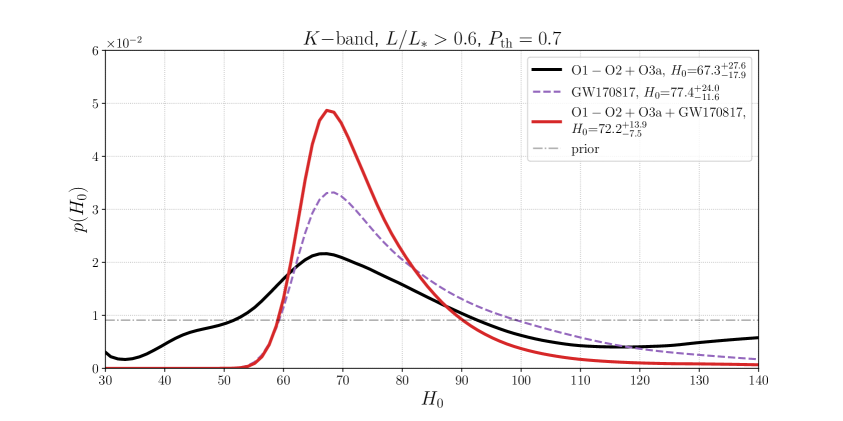
Figure 10: The posterior of $H_{0}$ obtained from GW170817 with its electromagnetic counterpart (violet dashed line), the posterior obtained from dark sirens in the O1+O2+O3a run obtained using mask completeness, multiplicative completion, K band, and $P_{\rm th}=0.7$ (black line, the same as the black lines in Figs. 6 and 7), and the combination of GW170817 and dark sirens (red solid line).

The results obtained combining O1+O2+O3a dark sirens with GW170817+counterpart are shown in Fig. 10, where we show, as before, the results for dark sirens is obtained using mask completeness, multiplicative completion, K band luminosity weighting, and a threshold on completeness $P_{\rm th}=0.7$. We see that the posterior of GW170817+counterpart falls to zero well before the upper limit of the prior range, and induces a similar behavior on the combined posterior. It therefore makes sense to quote the median of the posterior distribution. Using GW170817 alone, for the median and symmetric $68.3\%$ credible interval we find

$$H_{0}={77.4^{+24.0}_{-11.6}}\,\,\,{\rm km}\,{\rm s}^{-1}\,{\rm Mpc}^{-1}\,,\quad\quad\mbox{\small(GW170817 only)}\,.\\$$ (4.7)

This is consistent with the value $H_{0}=74^{+16}_{-8}\,{\rm km}\,{\rm s}^{-1}\,{\rm Mpc}^{-1}$ (again median and symmetric $68.3\%$ credible interval) obtained in ref. [18] using a prior proportional to $d_{L}^{2}$, a flat-in-log prior on $H_{0}$, and the value of the recession velocity of NGC4993 discussed above.

Combining the posterior from GW170817 with that from dark sirens, we get

$$H_{0}={72.2^{+13.9}_{-7.5}}\,\,{\rm km}\,{\rm s}^{-1}\,{\rm Mpc}^{-1}\,,\quad\quad\mbox{\small(GW170817+dark sirens) }\,.$$ (4.8)

We see that the addition of dark sirens provides a non-negligible improvement on the accuracy of the measurement of $H_{0}$. Equation (4.8) corresponds to a relative error on $H_{0}$ of $15\%$, to be compared with the relative error of $23\%$, obtained from eq. (4.7), using GW170817 only. Equation (4.8) also improves on the result $H_{0}=70^{+20}_{-9}\,{\rm km}\,{\rm s}^{-1}\,{\rm Mpc}^{-1}$, which corresponding to $21\%$ error, obtained in [34] from GW170817 and dark sirens from O1-O2 (using again a flat prior on $H_{0}$, as in our case). To compare with [34], we also report the result that we obtain from GW170817+dark sirens using a uniform in log prior on $H_{0}$, $H_{0}=70.9^{+12.2}_{-6.8}\,\,{\rm km}\,{\rm s}^{-1}\,{\rm Mpc}^{-1}$, corresponding to a $13\%$ error. This should be compared with the value $H_{0}=69^{+16}_{-8}\,\,{\rm km}\,{\rm s}^{-1}\,{\rm Mpc}^{-1}$ obtained in [34]. However, for $H_{0}$, our prior information from cosmological observations does not span several orders of magnitudes, so a prior uniform in $H_{0}$ is more justified than a prior uniform in $\log H_{0}$.

The above results were obtained without any modelization of the jet emission from GW170817, and rely only on the fact that standard sirens provide an absolute measurement of the luminosity distance. Therefore, they are purely ‘gravitational’ results. However, Very Long Baseline Interferometry (VLBI) constrains the emission angle of the jet associated to the EM counterpart of GW170817 [116]. In particular, one can constrain the viewing angle $\Theta=\min(\theta_{\rm{JN}},\pi-\theta_{\rm{JN}})$, where $\theta_{\rm{JN}}$ is the angle between the line of sight and the total angular momentum of the binary [2], as

$$0.25\,{\rm rad}\leq\left(\frac{d_{L}}{41\,\rm{Mpc}}\right)\Theta\,\leq 0.45\,{\rm rad}\,.$$ (4.9)

For small spins of the individual binaries and negligible precession of the orbital plane, as in the case of GW170817, $\theta_{\rm{JN}}\simeq\iota$ where $\iota$ is the inclination angle, so this information can be used to break the degeneracy between the distance and the inclination of the orbit. One then obtains a significantly tighter measurement of the Hubble parameter, $H_{0}=68.3^{+4.6}_{-4.5}\,{\rm km}\,{\rm s}^{-1}\,{\rm Mpc}^{-1}$ [114]. Of course, one must stress that this result is based on some jet modeling, which could potentially introduce extra uncertainties and systematic errors.

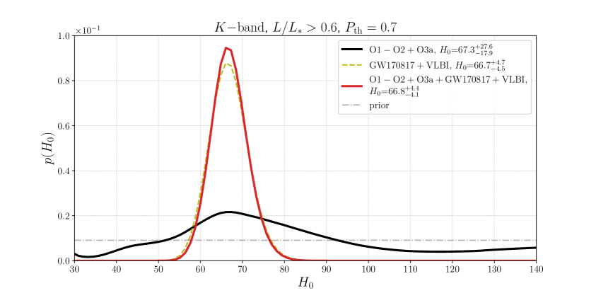
Figure 11: As in Fig. 10, adding the VLBI information on GW170817.

In any case, it is obviously interesting to combine this result with dark sirens. First of all, we have repeated the analysis for GW170817 using the VLBI constraint, by selecting only the posterior samples in the interval (4.9), finding $H_{0}=66.7^{+4.7}_{-4.5}\,{\rm km}\,{\rm s}^{-1}\,{\rm Mpc}^{-1}$, consistent with [114]. We have then combined it with the dark sirens posterior. The results are shown in Fig. 11, using again mask completeness, multiplicative completion, K-band, and $P_{\rm th}=0.7$. We see that, in this case, given that the posterior from GW170817 alone becomes much more narrow, combining it with the posteriors from current dark sirens gives only a very marginal improvement. Our result, from GW170817 with VLBI plus dark sirens, is

$$H_{0}=66.8^{+4.4}_{-4.1}\,\,{\rm km}\,{\rm s}^{-1}\,{\rm Mpc}^{-1}\quad\mbox{\small(GW170817+VLBI+dark\, sirens) },$$ (4.10)

corresponding to a measurement of $H_{0}$ at the $6.3\%$ level. By comparison, the Planck value is $H_{0}=67.4^{+0.5}_{-0.5}\,{\rm km}\,{\rm s}^{-1}\,{\rm Mpc}^{-1}$ [21] and the SH0ES value is $H_{0}=74.0^{+1.4}_{-1.4}\,{\rm km}\,{\rm s}^{-1}\,{\rm Mpc}^{-1}$ [19] (which becomes $H_{0}=73.8^{+1.1}_{-1.1}\,{\rm km}\,{\rm s}^{-1}\,{\rm Mpc}^{-1}$ when combined with H0LiCOW [20]). The result (4.10) slightly favors the Planck result. However, the error is still quite large (with both the SH0ES and the combined SH0ES+H0LiCOW results still within $1.5\sigma$), and one should also keep in mind the potential uncertainty due to possible systematics in the jet modelization, so that no definite conclusion can yet be drawn.

4.2 Modified GW propagation

We now repeat the analysis for modified GW propagation. As discussed in sect. 3.1 (see also footnote 9 on page 9), in this case we will fix $H_{0}$ to the value $H_{0}=67.88\,\,{\rm km}\,{\rm s}^{-1}\,{\rm Mpc}^{-1}$, which is the mean value obtained from a fit to CMB+BAO+SNa data, both in the $\Lambda$CDM and in the RT nonlocal model with large $\Delta N$ (and letting the sum of neutrino masses vary freely within the observational limits). In principle, a more correct approach would be to let both $H_{0}$ and $\Xi_{0}$ free, with a prior on $H_{0}$ fixed by the CMB+BAO+SNa data. However, CMB+BAO+SNa data fix $H_{0}$ to a precision of about $0.7\%$ while, as we will see, the bounds that we will obtain on $\Xi_{0}$ will rather be in the range $\Xi_{0}<{\cal O}(5)$, i.e. a deviation of order $500\%$ from the GR value $\Xi_{0}=1$. With current data, therefore, the degeneracy with $H_{0}$ can be neglected. We will also fix $n$ in eq. (2.7) to the value $n=1.91$, which is the value predicted by the RT model in the RT nonlocal model with large $\Delta N$, but this choice has a limited impact on our analysis, and similar results are obtained as long as $n={\cal O}(1)$.

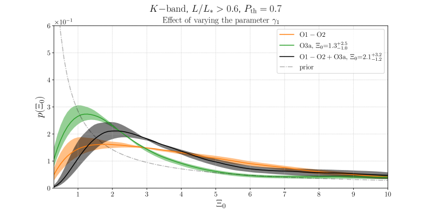
Figure 12: The separate posterior for $\Xi_{0}$ from the O1+O2 data and from the O3a data, and their combined posterior (using mask completeness, multiplicative, completion, $P_{\rm th}=0.7$, K-band luminosity weighting, and a prior uniform in $\log\Xi_{0}$). The shaded bands give the effect of changing $\gamma_{1}$ within the range $\gamma_{1}=1.05^{+0.68}_{-1.08}$.

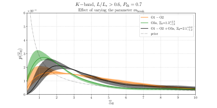
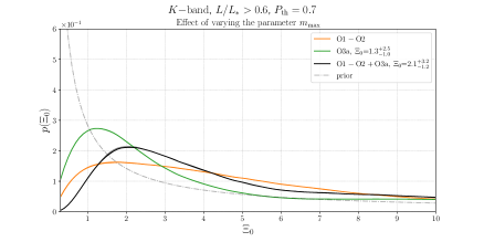
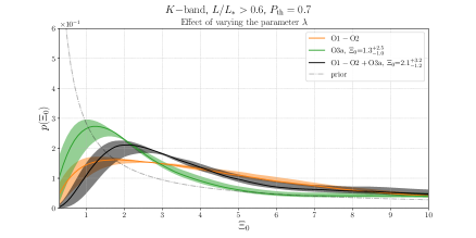
Figure 13: Upper row: the effect of changing $m_{\rm break}$ within the range $m_{\rm break}=36.76^{+11.37}_{-12.48}\,M_{\odot}$ (left panel) and the effect of changing $m_{\rm max}$ within the range $m_{\rm max}=86.16^{+12.37}_{-13.65}\,M_{\odot}$ (right panel). Lower panel: the effect of changing $\lambda$ in eq. (3.110) within the range $[0,3]$, with the central lines corresponding to our default value $\lambda=1$. We use mask completeness, multiplicative completion, K band, and a completeness threshold $P_{\rm th}=0.7$.

For the Hubble constant, we have used a prior uniform in $H_{0}$. This is the most natural choice, given that electromagnetic observations already constrain $H_{0}$ significantly. In contrast, as we reviewed in sect. 2.3, current limits on $\Xi_{0}$ are very broad. We will therefore use a correspondingly broad prior range $\Xi_{0}\in[0.3,10]$. In such a range, that extends over almost two orders of magnitude, a more natural choice is a prior uniform in $\log\Xi_{0}$, rather than in $\Xi_{0}$. In the following, we will therefore always use a uniform-in-log prior for $\Xi_{0}$. Since $d\log\Xi_{0}=d\,\Xi_{0}/\Xi_{0}$, with respect to a prior uniform in $\Xi_{0}$ this has the effect of suppressing the tails of the posterior at large $\Xi_{0}$. As discussed in App. E, the more stringent prior knowledge that we have on $H_{0}$ allowed us to determine the best settings for our baseline model. We will then use exactly the same settings for $\Xi_{0}$, namely mask completeness, multiplicative completion, $P_{\rm th}=0.7$ and K-band luminosity weighting.

In Fig. 12 (which is the analogous of Fig. 6 for $H_{0}$) we show the posteriors for $\Xi_{0}$ from the O1-O2 data, the O3a data, and the total posterior obtained by combining the O1+O2 data with the O3a data. As in Fig. 6, the central lines in the shaded bands give the posteriors for $\gamma_{1}=1.05$, while the shaded bands give the effect of varying $\gamma_{1}$ in the interval $\gamma_{1}=1.05^{+0.68}_{-1.08}$. For the maximum a posteriori value and its corresponding highest density interval, from the combined O1+O2+O3a data, we get

$$\Xi_{0}=2.1^{+3.2}_{-1.2}\,.$$ (4.11)

The effect of changing $\gamma_{1}$ in the BBH mass function, within the limits $\gamma_{1}=1.05^{+0.68}_{-1.08}$, can be appreciated from the shaded bands in Fig. 12. In Fig. 13 we show the effect of changing $m_{\rm break}$, $m_{\rm max}$ and $\lambda$, similarly to the plots made for $H_{0}$ in Fig. 8. We observe that changing $m_{\rm max}$ (at fixed $m_{\rm break}$) has almost no effect. The effect of changes in $\lambda$ on the posterior of $\Xi_{0}$ is less pronounced, compared to its effect on the posterior of $H_{0}$, and about comparable to that of changes in $m_{\rm break}$ and $\gamma_{1}$.

The individual contributions from the five events in O1+O2+O3a that pass the completeness threshold $P_{\rm th}=0.7$ are shown in Fig. 14. Similarly to what we found for $H_{0}$, the single most significant contribution comes from GW190814, but all other events contribute to the total posterior.

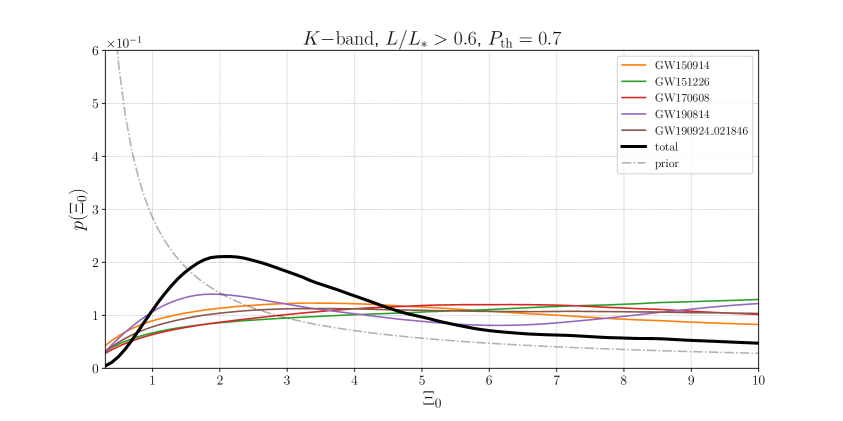
Figure 14: The separate contributions to the posteriors of $\Xi_{0}$, from the individual events in O1+O2+O3a that pass the completeness threshold $P_{\rm th}=0.7$. The black line is the total posterior from O1+O2+O3a, already shown as the line inside the black band in Fig. 12.

4.3 GW190521 and its candidate counterpart

One of the most interesting detections in the O3a run is the BBH GW190521 [119, 120]. Assuming a quasi-circular orbit, it is interpreted as the coalescence of two BHs with masses $85^{+21}_{-14}$ and $66^{+17}_{-18}M_{\odot}$. One reason that makes this event remarkable is that, because of the pulsational pair-instability supernova mechanism, it is believed that no BH should form from stellar collapse in the approximate mass range $\sim(65-135)M_{\odot}$. The primary BH mass in GW190521 lies in this mass gap, with only $0.32\%$ probability of being below $65M_{\odot}$. The inferred mass of the final BH is $142^{+28}_{-16}M_{\odot}$, which classifies it as the first observation of an intermediate mass BH. Another remarkable property of this event is its luminosity distance, estimated to be $d_{L}\simeq 5.3^{+2.4}_{-2.6}$ Gpc, making it currently the farthest GW detection. In $\Lambda$CDM, and assuming a Planck cosmology, the corresponding redshift is $z=0.82^{+0.28}_{-0.34}$. However, a main theme of this paper is that in modified gravity this luminosity distance becomes a GW luminosity distance and the redshift will be different, and we will elaborate on this below.

Ref. [70] has proposed a potential electromagnetic counterpart to this GW detection, consisting of an electromagnetic flare detected by the Zwicky Transient Facility, labeled ZTF19abanrhr. The flare is associated with an AGN at $z=0.438$ and could be interpreted as due to the remnant BH, which has been kicked by the merger and is moving at high speed through the accretion disk of the AGN, according to a model previously proposed in ref. [121]. As we already mentioned in sect. 2.3, doubts have been raised on this association. One aspect of the problem is that it is not currently clear how plausible is the model for an AGN flare from a kicked BH, and on this issue we will have nothing to add. On top of this, in ref. [71] it has been argued that the probability of a real association based on volume localization is not statistically sufficient for a confident identification of ZTF19abanrhr as the counterpart. This analysis, however, is based on the redshift determination of the GW event made using GR and $\Lambda$CDM. In modified gravity the situation is different, and the comparison of the GW posterior on the luminosity distance, that in this case is a GW luminosity distance, with the redshift of the candidate counterpart, can be translated into a posterior for $\Xi_{0}$. It is therefore interesting to reanalyze the possible association with the counterpart, in the context of modified GW propagation. A similar analysis has already been done in [72], using various parametrization of modified GW propagation including our eq. (2.7), while in [115] the event as been studied in the context of $w$CDM, and we will compare below with their results.

We consider again a likelihood of the form (4.2), with the likelihood for the EM measurement given by eq. (4.3), and we will study both the posterior for $H_{0}$ in the framework of $\Lambda$CDM, obtained from GW190521 assuming that ZTF19abanrhr is indeed the counterpart, and the corresponding posterior for $\Xi_{0}$ in the framework modified gravity. As discussed after eq. (3.2), when we study the Hubble parameter in the context of $\Lambda$CDM we fix all other cosmological parameters to the mean values obtained from CMB+BAO+SNe; similarly, when we study modified GW propagation, we keep $\Xi_{0}$ as the only free parameter and we fix all other cosmological parameters, including $H_{0}$, to their mean values obtained from CMB+BAO+SNe. Indeed, we will see below that, also in the case of GW190521+ZTF19abanrhr, just as for dark sirens, the limits that one can currently obtain on $\Xi_{0}$ are still very broad, allowing variation of about a factor of 3, i.e. of about $300\%$, or more compared to the value $\Xi_{0}=1$ of GR. Then, letting $H_{0}$ vary within a prior consistent with CMB+BAO+SNe data, which fix it to an accuracy at the $0.7\%$ level, would have a negligible effect, compared to fixing it to the corresponding mean value; on the other hand, the current data have too little constraining power to provide useful limits if we do not use at all the CMB+BAO+SNe prior, and we attempt a purely gravitational measurement.

Since the candidate counterpart is at considerably higher redshift than in the case of GW170817, there is no significant effect from peculiar velocities, and we can now neglect the small uncertainty in the electromagnetic determination of the redshift. We therefore fix the position of the counterpart to $z_{\rm EM}=0.438$, $(\alpha_{\rm EM},\delta_{\rm EM})=(192.42625^{\circ},34.82472^{\circ})$ [70]. As for the prior on masses, as explained in sect. 4.1.2, one should in principle re-weight the samples to include the correct mass distribution, which can also induce a dependence on the cosmology through the conversion between source and detector frame masses (see also footnote 14 on page 14). However, the choice of a mass function for GW190521 is a subtle point. First, as discussed above, when analysed with a standard flat prior in detector frame mass, this event has a reported primary mass that lies inside the pair instability Supernovae mass gap, and at the edge of all the best-fit primary mass distributions discussed in [105], including the broken power-law used in this work, eq. (3.102), which makes it difficult to efficiently re-sample the LVC posterior samples. Moreover, large uncertainties are still associated to all such mass distributions, which become relevant for such an extreme event. Additionally, it has been argued that the use of a population-informed prior on the secondary mass in the analysis could change substantially the inferred values for the parameters [122], and that this event could be a highly eccentric merger, which also gives different values for the component masses [123]. In conclusion, we make the standard choice of not re-weighting the LVC samples, which corresponds to the use of a prior flat in detector frame mass in the range $[30-100]\,M_{\odot}$ [120, 115, 72, 6]. It must, however, be kept in mind that the use of a proper mass function can have a large impact on the final result. As prior for the distance we choose $\tilde{p}_{0}(z)$ as in eq. (3.110) with $\lambda=0$, which corresponds to a merger rate uniform in comoving volume and source-frame time (this is the same prior used in the LVC analysis of O3a data, see sect. V.C of [6])

With the above assumptions, the calculation of the posterior for this event reduces to the computation of the line-of-sight marginal likelihood $p({\cal D}_{\rm GW}|d_{L},\hat{\Omega}_{\rm EM})$. The LVC provides posterior samples obtained by using four different waveform models. In Fig. 15 we show our reconstruction of the marginalized likelihood in the direction of the counterpart, $p({\cal D}_{\rm GW}|d_{L},\hat{\Omega}_{\rm EM})$, for the four waveforms.

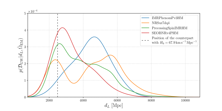
Figure 15: The line-of-sight marginal likelihood in the direction of the counterpart, $p({\cal D}_{\rm GW}|d_{L},\hat{\Omega}_{\rm EM})$, for the four different waveform models used by the LVC. The dotted vertical line represents the position of the counterpart for $H_{0}=67.9\,{\rm km}\,{\rm s}^{-1}\,{\rm Mpc}^{-1}$ and $\Xi_{0}=1$.

We first compute the posterior of $H_{0}$ in $\Lambda$CDM obtained from GW190521 assuming that ZTF19abanrhr is indeed the counterpart. To compute $\beta(H_{0})$ we use our MC in the absence of additional selection effects given by the incompleteness of the catalog, using the O3 strain sensitivity, the broken power law eq. (3.102) for the mass distribution, and neglecting any EM contribution to the selection effect.

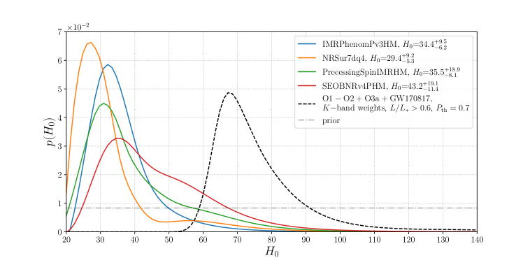
Figure 16: Posterior distributions for $H_{0}$ obtained from GW190521 and its potential EM counterpart for four different waveforms. For comparison, we show also the posterior obtained in the previous section combining GW170817 with dark sirens.

The resulting posterior distribution for $H_{0}$ is shown in Fig. 16, for the four waveform models provided by the LVC. By comparison, we plot it together with the posterior that we obtained by combining GW170817 with dark sirens, already shown as the red line in Fig. 10. Even if the statistical error is large and the difference can be accounted as a statistical fluctuations, we see that, independently of the waveform model used, the posterior for $H_{0}$ from GW190521+counterpart is in tension with the value of $H_{0}$ that we already know from electromagnetic observations, whether we use the Planck value $H_{0}=67.4^{+0.5}_{-0.5}\,{\rm km}\,{\rm s}^{-1}\,{\rm Mpc}^{-1}$ [21], or the even larger SH0ES value $H_{0}=74.0^{+1.4}_{-1.4}\,{\rm km}\,{\rm s}^{-1}\,{\rm Mpc}^{-1}$ [19], contrary to the result obtained from dark sirens together with GW170817+counterpart (black dotted line), which is fully consistent with them.

Apart from the possibility of a statistical fluctuation, within $\Lambda$CDM two possible interpretations are either that ZTF19abanrhr is simply not the counterpart, or that the estimate of the luminosity distance is not correct because the binary had a significant eccentricity. Indeed, as discussed in [120], the signal only stays in the detector bandwidth for about four cycles (as a consequence of the large mass of the system) so that, while considered the most plausible, the interpretation in terms of a quasi-circular coalescence is not certain. Using a model in which GW190521 was a highly eccentric BBH with eccentricity $e\sim 0.7$, and assuming that ZTF19abanrhr is the counterpart, ref. [123] finds $H_{0}=88.6^{+17.1}_{-34.3}\,{\rm km}\,{\rm s}^{-1}\,{\rm Mpc}^{-1}$, consistent with standard cosmology within the very large error.

Another obviously interesting possibility is to analyze the possible association between GW190521 and ZTF19abanrhr by enlarging the cosmological model, with respect to $\Lambda$CDM. An investigation in this direction has been done in [115], that considers $w$CDM, i.e. the phenomenological extension of $\Lambda$CDM where the DE equation of state is taken to be a constant $w_{0}$, while perturbations are assumed to be the same as in $\Lambda$CDM. In this case, assuming that ZTF19abanrhr is the counterpart and varying also $\Omega_{M}$, the result of ref. [115] is $H_{0}=48^{+23}_{-10}\,{\rm km}\,{\rm s}^{-1}\,{\rm Mpc}^{-1}$, $\Omega_{M}=0.35^{+0.41}_{-0.26}$ and $w_{0}=-1.31^{+0.61}_{-0.48}$ (median and $68\%$ credible interval). However, as we discussed in sect. 2.3, current limits from electromagnetic observations show that $w_{0}$ cannot differ from $-1$ by more than about $5\%$ and, using this as a prior, the result for $H_{0}$ from GW190521+ZTF19abanrhr obtained in $w$CDM would not be significantly different from that in $\Lambda$CDM. More importantly, as discussed in sect. 2, any known model that deviates from $\Lambda$CDM at the background level, giving a DE equation of state different from $w=-1$, also predicts modified GW propagation, and the effect of modified GW propagation in general dominates, possibly even by 1-2 orders of magnitude, over that induced by the DE equation of state, because: (1) in viable models $w_{0}$ is constrained to be equal to $-1$ within a few percent, while $\Xi_{0}$ can have large deviations from the GR value $\Xi_{0}=1$, with known examples where $\Xi_{0}$ can be as large as $1.80$; and, (2) the effect of $\Xi_{0}$ on the luminosity distance is more important than the effect of $w_{0}$ because of degeneracies among $H_{0}$, $\Omega_{M}$ and $w_{0}$, see the discussion on page 2. For these reasons, opening the parameter space by including $w_{0}$, while neglecting modified GW propagation, does not appear well justified. Here we will rather pursue the opposite strategy, investigating the effect of $\Xi_{0}$ in a model where the electromagnetic luminosity distance differs little from that in $\Lambda$CDM, see also the discussion at the beginning of sect. 2.4.

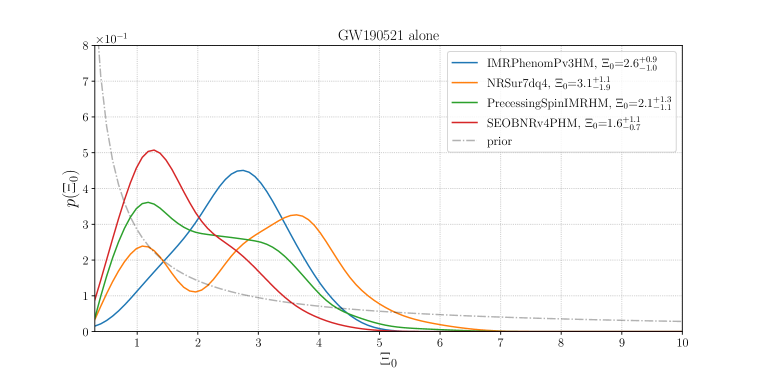
Figure 17: Posterior distributions for $\Xi_{0}$ obtained from GW190521 and its potential EM counterpart for four different waveform models.

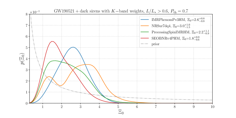
Figure 18: Posterior distribution for $\Xi_{0}$, combining GW190521 and dark sirens using K-band weights, and a threshold probability $P_{\rm th}=0.7$.

Proceeding as we have done for $H_{0}$, but keeping now $\Xi_{0}$ as the only free parameter, we find the posteriors shown in Fig. 17, for the four waveform models. The corresponding limits on $\Xi_{0}$ for the four waveform are given in Table 3 (median values and limits at $68.3\%$ and $95\%$ credible interval).

	NRSur	IMRPhenom	SEONBR	PrecessingSpin
$\Xi_{0}\,(68.3\%)$	$3.1^{+1.1}_{-1.9}$	$2.6^{+0.9}_{-1.0}$	$1.6^{+1.1}_{-0.7}$	$2.1^{+1.3}_{-1.1}$
$\Xi_{0}\,(95\%)$	$3.1^{+2.4}_{-2.5}$	$2.6^{+1.7}_{-1.8}$	$1.6^{+2.3}_{-1.1}$	$2.1^{+2.6}_{-1.6}$

Table 3: Median value and limits on $\Xi_{0}$ ($68.3\%$ and $95\%$ symmetric credible interval), for the four waveform models, from GW190521+ZTF19abanrhr.

	NRSur	IMRPhenom	SEONBR	PrecessingSpin
( $\Xi_{0}\,(68.3\%)$	$3.0^{+1.0}_{-1.5}$	$2.6^{+0.8}_{-0.8}$	$1.8^{+0.9}_{-0.6}$	$2.2^{+1.1}_{-0.9}$
( $\Xi_{0}\,(95\%)$	$3.0^{+2.1}_{-2.1}$	$2.6^{+1.6}_{-1.5}$	$1.8^{+1.9}_{-1.1}$	$2.2^{+2.2}_{-1.4}$

Table 4: Median value and limits on $\Xi_{0}$ ($68.3\%$ and $95\%$ symmetric credible interval), for the four waveform models, from GW190521+ZTF19abanrhr combined with dark sirens (using K-band, with a completeness threshold $P_{\rm th}=0.7$).

These results can be compared with those in Table 1 of ref. [72], where the limits are given at $95\%$ credible interval. The results are broadly consistent. However, ref. [72] only obtains upper limits on $\Xi_{0}$, while the results in our Table 3 provide both upper and lower limits on $\Xi_{0}$.^,

Contrary to what happens for $H_{0}$ in $\Lambda$CDM, see fig. 16, the posterior for $\Xi_{0}$ obtained from GW190521+ZTF19abanrhr is consistent with that obtained from dark sirens found in sect. 4.2, and therefore it makes sense to combine them. In Fig. 18 we show the total posterior obtained by combining the result from GW190521+ZTF19abanrhr (with the four waveform models) with the dark sirens posterior that we obtained in sect. 4.2 from O1+O2+O3a data (using K-band weights and a threshold probability $P_{\rm th}=0.7$). The corresponding limits on $\Xi_{0}$ for the four waveform are given in Table 4. The best bound depends on the waveform used, with the most stringent one being

$$\Xi_{0}=1.8^{+0.9}_{-0.6}\,,$$ (4.12)

(median and $68.3\%$ credible interval), obtained from GW190521+ZTF19abanrhr with SEOBNRv4PHM waveform, combined with dark sirens.

Observe that the ‘tension’ that, in the context of $\Lambda$CDM, exists between the spatial localization of GW190521 and the redshift of ZTF19abanrhr, and which has led to doubts on the interpretation of ZTF19abanrhr as the counterpart to GW190521 [70], once interpreted in the context of modified gravity translates into a (small) tension between the measured value of $\Xi_{0}$ in eq. (4.12) and the GR value $\Xi_{0}=1$. To interprete correctly this result, however, one must stress that the association of ZTF19abanrhr with GW190521 is anyhow tentative. Furthermore, the statistical error in eq. (4.12) is large, so that the GR value is still at the border of the $68\%$ credible interval. We have also seen that there is a large uncertainty due to different waveform models, as apparent from Fig. 18, and one must also take into account the possibility of explaining the low value of $H_{0}$ obtained from GW190521+ZTF19abanrhr within $\Lambda$CDM in terms of a large eccentricity [123]. Therefore, the result (4.12) should obviously be interpreted with care. It shows, however, the potential of standard sirens for obtaining interesting limits on $\Xi_{0}$.

5 Conclusions

In this paper we have first of all developed several methodological aspects relevant for performing statistical correlations of dark sirens with galaxy catalogs, paying special attention to many systematic errors, and to the effect of various choices that are made in the analysis. This will become more and more important as GW detectors increase their range and collect more and more events at high redshift, and will be even more important for third generation (3G) ground based interferometers such as the Einstein Telescope and Cosmic Explorer, as well as for the LISA space interferometer.

We have introduced and compared two different ‘quasi-local’ ways of quantifying the level of completeness of a galaxy catalog (cone completeness and mask completeness) and, given an assessment of the level of completeness, we have compared the results from two different ways of distributing the missing galaxies, the ‘homogeneous completion’, previously used in the literature, and the ‘multiplicative completion’, that we have proposed here. The latter can be seen as a quantitative realization of the intuitive idea that, for the GW/galaxy correlation, it is sufficient that a galaxy catalog traces the structure of galaxy clusters.

We have compared the results with different luminosity weightings, and with different astrophysical assumptions, as encoded for instance in the parameters that enters the BBH mass function (3.102) or in the parameter $\lambda$ that parametrizes the redshift dependence of the mass function, eq. (3.110). Eventually, the only way forward will be to turn some of the systematic uncertainties, at least the ones regarding the unknown mass and redshift distribution of BBH sources, into statistical uncertainties, and jointly fit for the population and cosmology.

We have paid special attention to the computation of the function $\beta(H_{0})$ that enters in eq. (3.10), using different levels of refinement. Another delicate point that emerged from our analysis is the need of including a completeness threshold on the events, that must be carefully accounted for in the computation of $\beta(H_{0})$. We have seen that there can be a significant dependence on this threshold, and that large values of this threshold are necessary to avoid the possible introduction of spurious effects. All these technical details turn out to be quite crucial if one eventually aims at measuring $H_{0}$ with percent level precision from dark sirens. Current data are still limited by statistics, but the results that we have presented show that, eventually, to reach such a precision, these systematic effects must be well understood, and our paper is meant first of all as a contribution in this direction.

Apart from the methodological aspects, the application to current data is already quite interesting, even if still clearly limited by the statistics and by the fact that, with the current detector network, the localization of GW events is very broad. Our best result from dark sirens only, for $H_{0}$, is shown in Fig. 6 and in eq. (4.1), and provides the currently most accurate results obtained from standard sirens only, while Fig. 10 and eqs. (4.7) and (4.8) show how the addition of dark sirens from the O1, O2 and O3a runs improves the constraint on $H_{0}$ obtained from GW170817 and its counterpart.

While, in the literature, most of the work on dark sirens has been currently focused on extracting $H_{0}$, we have stressed that, eventually, the most interesting contribution that GW observations can give to cosmology might be the observation of modified GW propagation, which is a smoking gun of dark energy and modified gravity, and can only be observed with GW detectors. We have presented our result in terms of $\Xi_{0}$, the main parameter that characterizes modified GW propagation, and we find that, even with the current limited statistics, dark sirens start to provide interesting limits. Our best results, using dark sirens only, are given by Fig. 12 and eq. (4.11).

Finally, we have considered the limits that can be obtained on modified GW propagation if one accepts the interpretation of the flare ZTF19abanrhr as the electromagnetic counterpart of the BBH coalescence GW190521 (assumed to be in a quasi-circular orbit). In this case, combining the result from GW190521 with the posterior from dark sirens, our most stringent result is given in eq. (4.12). Considering that, in nonlocal gravity with initial conditions in inflation, the prediction for $\Xi_{0}$ is in range $\Xi_{0}\simeq 1.6-1.8$ [60, 61], to be compared with $\Xi_{0}=1$ for GR, the result in eq. (4.12) is suggestive. However, because of the various caveats discussed in sect. 4.3, one cannot yet draw any conclusion, except that, with the expected increase in the amount and quality of the GW data, modified GW propagation can become an extremely interesting observable for GW observations.

Together with this paper, we release the publicly available code $\tt{DarkSirensStat}$, which is available under open source license at https://github.com/CosmoStatGW/DarkSirensStat.

Acknowledgments. We are grateful to Enis Belgacem for his contributions to the early stages of this work, and for many useful discussions. We thank Gergely Dálya, Archisman Ghosh, Ignacio Hernandez and Simone Mastrogiovanni for very useful discussions, and the referee for an extremely competent, careful and useful report. The work of the authors is supported by the Swiss National Science Foundation and by the SwissMap National Center for Competence in Research.

Appendix A Completeness of the GLADE catalog

In this appendix we discuss in some detail the completeness of the GLADE catalog (complementing the discussion in [99] and in [31]), both as an application of the tools developed in sect. 3.2, and for its intrinsic usefulness for the results that we present in the paper. This will also allow us to fix our choices for the parameters $\Delta z$, $\Delta\Omega$ that appear in the cone completeness $P_{\rm compl}^{\rm cone}(z,\hat{\Omega};\Delta z,\Delta\Omega)$ and to test mask completeness, and to select a choice of weights and of luminosity cuts. For definiteness, we will illustrate our results using cone completeness, which is more intuitive, but similar results are obtained from mask completeness (that, as we saw from Tables 1 and 2 in sect. 4.1.1, produces slightly higher values of the completeness).

Completeness strongly depends on the weights used, and on the direction of the sky. The upper panels of Fig. 19 show the distribution of galaxies with $0<z<0.2$ (upper left panel) and with $0<z<1$ (upper right panel) in the GLADE catalog, assigning a weight $w_{\alpha}=1$ to each galaxy and using galactic coordinates. Besides the cut in the Galactic plane, are clearly visible stripes (arising from the HyperLEDA catalog) and regions that have been much better covered than others, corresponding to the footprints of the various surveys that contribute to GLADE. From these plots, it is clear that a notion of completeness defined by integrating over $4\pi$, as used until now in the literature, is very approximate, and the angular-dependent completeness that we have introduced is more appropriate.

The lower panel of Fig. 19 is the same as the upper right panel, except that the plot is shown in equatorial coordinates (RA, dec), and we have marked by a cross the points with RA=0 and ${\rm dec}=\{60,30,-30,-60\}$. We see that the directions with RA=0 and ${\rm dec}=\{30,-30\}$ are examples of well-covered directions, while RA=0 and ${\rm dec}=\{60,-60\}$ are examples of directions with lesser coverage, and we will use them below, to illustrate the behavior of the completeness in different directions.

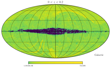
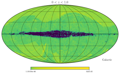
Figure 19: Upper panels: the distribution of galaxies in the GLADE catalog, in galactic coordinates, on a logarithmic scale, using weights $w_{\alpha}=1$. Left panel: the galaxies with $0<z<0.2$. Right panel: the galaxies with $0<z<1$. Lower panel: the same as the upper right panel, now in equatorial coordinates, and with the directions with RA=0 and ${\rm dec}=\{60,30,-30,-60\}$ marked by a cross.

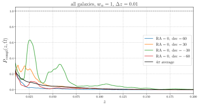
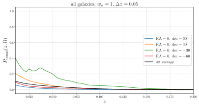
Figure 20: The function $P_{\rm compl}(z,\hat{\Omega})$ using all galaxies in GLADE and no luminosity weighting, i.e. $w_{\alpha}=1$, for the four directions $\hat{\Omega}$ corresponding to the crosses in the lower panel of Fig. 19 (colored lines) and the all-sky average (black line). The colored line are obtained using sections of cones with half-opening angle $\theta_{c}=5^{\circ}$. The black line is the $4\pi$ average. Left panel: using, in the radial direction, a section of a cone with $\Delta z=0.01$. Right panel: the same, with $\Delta z=0.05$.

Using $w_{\alpha}=1$ we can make use of all galaxies in the catalog (GLADE contains about 2.7 millions galaxies, of which 1.6 millions have a known B-band luminosity, and 1.0 millions have a known K-band luminosity; practically all galaxies with known K-band luminosity also have a known B-band luminosity).^,

However, in this case the catalog becomes quickly very incomplete with distance, since we miss most of the low-luminosity galaxies, and, with this weighting, a low-luminosity galaxy counts as much as a high-luminosity one. This is clearly visible from Fig. 20 that shows, as a function of $z$, the function $P_{\rm compl}(z,\hat{\Omega};\Delta z,\Delta\Omega)$ defined in eq. (3.49) (setting $\bar{n}_{\rm gal}=0.1\,{\rm Mpc}^{-3}$), with ${\cal S}(z,\hat{\Omega};\Delta z,\Delta\Omega)$ given by a section of a cone with axis $\hat{\Omega}$ and half-opening angle $\theta_{c}$ [so $\Delta\Omega=2\pi(1-\cos\theta_{c})$], and restricted, in the radial direction, to redshifts between $z-(\Delta z/2)$ and $z+(\Delta z/2)$. The four colored lines correspond to cones whose axis $\hat{\Omega}$ is given by the four directions marked with a cross in the lower panel of Fig. 19. We see that the curves corresponding to directions that visually had better coverage, indeed have higher values of $P_{\rm compl}(z,\hat{\Omega};\Delta z,\Delta\Omega)$. Figs. 19 and 20 are complementary: Fig. 20 gives more detailed information on the redshift dependence, which appears only in integrated form in Fig. 19, but only for a few selected directions, while Fig. 19 shows the full angular dependence.

The colored curves in the left panel of Fig. 20 have been obtained by setting $\theta_{c}=5^{\circ}$ and $\Delta z=0.01$, while those in the right panel correspond to $\theta_{c}=5^{\circ}$ and $\Delta z=0.05$. The choice $\theta_{c}=5^{\circ}$ is suggested by the fact that it is much smaller than the typical angular localization of GW events, and also sufficiently small to resolve the region of the galactic plane which is obscured by dust, where completeness drop dramatically, so that we do not significantly mix regions close to the galactic plane with good covering, with the region near the galactic plane that is plainly obscured. In both panels, the black line is the average of the completeness over the whole sky, i.e. the quantity $P_{\rm compl}(z)$ defined by eq. (3.63).

The comparison of these two panels allows us, first of all, to appreciate the effect of the choice of $\Delta z$. As discussed in sect. 3.2.1, the optimal choice of $\Delta z$ (and of $\theta_{c}$) must be such that the region ${\cal S}$ is small enough, compared to the typical localization of GW events, to represent a ‘quasi-local’ property; still, it must be sufficiently large that the number of galaxies inside ${\cal S}$ (possibly with luminosity weighting) should be representative of the average value of galaxy number density (or, respectively, luminosity density), rather than being sensitive to true fluctuations such as actual voids or actual over-densities. A simple criterion to ensure the latter condition is that $P_{\rm compl}(z,\hat{\Omega};\Delta z,\Delta\Omega)$ should be a smoothly decreasing function of $z$, since the effect of having missed some galaxies because of observational limitations should produce a decreasing function of redshift, while actual overdensities and voids will be responsible for fluctuations over this smooth behavior. In the left panel, we see significant fluctuations superimposed to the smooth behavior. These clearly correspond to actual structures, i.e. under-densities and over-densities. As we see from the right panel, taking a larger $\Delta z$ smooths out these short-scale fluctuations. When we complete the catalog, we want to compensate for galaxies that have been missed because of observational limitations, but we certainly do not what to smooth out actual structures (that contains precisely the information that we need, in order to perform the correlation with the localization of the GW events). Therefore a binning that is too small, such as $\Delta z=0.01$, and that allows us to resolve true fluctuations in the galactic field, is not appropriate in the definition of $P_{\rm compl}(z,\hat{\Omega};\Delta z,\Delta\Omega)$. Using such an expression for $P_{\rm compl}$ would lead us to compensate these fluctuations, which represent actual over- or under-densities, as if they where due to short-scale variation (with respect to $z$) in the survey’s capability of detecting galaxies. It is only what remains after averaging over these fluctuations, by taking $\Delta z$ sufficiently large, that gives a measure of the fraction of galaxies that have been lost by the surveys. Thus, the binning must be sufficiently large so that $P_{\rm compl}(z,\hat{\Omega};\Delta z,\Delta\Omega)$ is a smooth and monotonically decreasing function of $z$. From the right panel we see that, for $w_{\alpha}=1$, this is the case for $\Delta z=0.05$ (except for the direction corresponding to the green curve, so one should actually take an even larger value of $\Delta z$). To have a sense for these choices of $\theta_{c}$ and $\Delta z$, in Fig. 21 we plot $V_{c}^{1/3}$ as a function of $z$, where $V_{c}$ is the comoving volume of a truncated cone with $\theta_{c}=5^{\circ}$ and redshift between $z-(\Delta z/2)$ and $z+(\Delta z/2)$, for the two choices $\Delta z=0.01$ and $\Delta z=0.05$. The cosmic web has typical structures on scales up to ${\cal O}(100)$ Mpc, with the largest cosmic voids having a size $\sim 50h_{0}^{-1}$ Mpc, and filaments stretching for tens of Mpc [125, 126]. Therefore, it is not surprising that the choice $\Delta z=0.01$, for which, for instance, $V_{c}(z=1)\simeq(190\,{\rm Mpc})^{3}$, is not sufficient to average over these structures. In contrast, for $\Delta z=0.05$ we have $V_{c}(z=1)\simeq(326\,{\rm Mpc})^{3}$, which appears more adequate to smooth out structures that can extend up to the 100 Mpc scale.

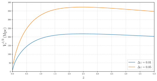
Figure 21: The quantity $V_{c}^{1/3}$ as a function of $z$, where $V_{c}$ is the comoving volume of a truncated cone with half-opening angle $\theta_{c}=5^{\circ}$ and redshift between $z-(\Delta z/2)$ and $z+(\Delta z/2)$, for the two choices $\Delta z=0.01$ and $\Delta z=0.05$.

Apart from obtaining an insight on the criterion for the optimal choice of $\Delta z$, what we learn from Fig. 19 is that, when using the weighting $w_{\alpha}=1$, the completeness of the GLADE catalog is quite poor already at $z\simeq 0.05$ (below $10\%$ for most directions, as shown by the $4\pi$ average, even having set $\bar{n}_{\rm gal}=0.1\,{\rm Mpc}^{-3}$, which is on the lower side of the estimate for $\bar{n}_{\rm gal}$), and at $z=0.10$ the catalog, with this weighting, is so incomplete that it is basically useless for our purposes. Therefore, except for events at very close distances, such as GW170817, we cannot get much information by correlating the localization of GW events with GLADE galaxies weighted with $w_{\alpha}=1$. In the following, we will therefore not use this weighting, when using GLADE.

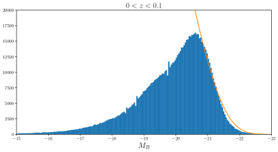
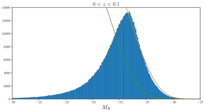
Figure 22: Left: the distribution in B-magnitude of the galaxies in the GLADE catalog compared to the Schechter function with parameters given in eq. (A.3) (yellow curve). Right: the same for K-band, with the Schechter function computed using the two choices of parameters discussed in the text, $M_{K}^{*}=-24.29$ (yellow curve) and $M_{K}^{*}=-23.55$ (green curve).

We then turn to luminosity weighting. First of all we observe that, for B band, the GLADE catalog provides both the measured apparent magnitudes of 1.6 millions galaxies, as well as their absolute magnitudes, that have been obtained, mostly from HyperLEDA, correcting for Galactic extinction, internal extinction (i.e., extinction within the galaxy in question) and K-correction (which corrects for the fact that the signal received in a given band was emitted in a different frequency range because of the frequency shift of the signal due to the cosmological or peculiar velocity of the source). In the left panel of Fig. 22 we show the distribution of GLADE galaxies with respect to the absolute B-band magnitude $M_{B}$ (considering for definiteness the range $0<z<0.1$). The yellow curve is the Schechter function (multiplied by the comoving volume out to redshift $z=0.1$) written in terms of magnitudes,

$$\phi(M_{B})=(0.4\ln 10)\phi_{B}^{*}\,\left[10^{0.4(M_{B}^{*}-M_{B})}\right]^{(1+\alpha_{B})}\,\exp\left[-10^{0.4(M_{B}^{*}-M_{B})}\right]\,,$$ (A.1)

which is obtained from eq. (3.76) using the standard relation between luminosity and absolute magnitude (in this case written for B-band quantities),

$$L_{B}=L_{B}^{*}\,10^{0.4(M_{B}^{*}-M_{B})}\,,$$ (A.2)

and requiring that $\phi(M)dM=\Phi(L)dL$, with $\Phi(L)dL$ given by eq. (3.76). For the Schechter parameters we used the values [127, 128, 99]

$$M_{B}^{*}=-20.47+5\log_{10}h_{0.7}\,,\qquad\phi_{B}^{*}=5.5\times 10^{-3}h_{0.7}^{3}\,{\rm Mpc}^{-3}\,,\qquad\alpha_{B}=-1.07\,,$$ (A.3)

where $h_{0.7}$ is $H_{0}$ in units of $70\,{\rm km}\,{\rm s}^{-1}\,{\rm Mpc}^{-1}$ (in the plots, we set $h_{0.7}=1$). Note that, plugging $L=L_{B,\odot}$ and $M=M_{B,\odot}$ in eq. (A.2), and using the value $M_{B,\odot}\simeq 5.498$ for the solar luminosity in B band, this corresponds to

$$L_{B}^{*}=2.45\,h_{0.7}^{-2}\,\times 10^{10}L_{B,\odot}\,.$$ (A.4)

We see from the figure that the Schechter function with these parameters (and $h_{0.7}=1$) fits reasonably well the high-luminosity tail of the distribution while, as expected, the low-luminosity part of the distribution of the galaxies in the GLADE catalog is well below the Schechter function, as a consequence of the fact that most low-luminosity galaxies are missed. This result is consistent with the plots in Fig. 3 of [99].

For K band, GLADE only provides the apparent magnitudes, from which we can obtain the absolute magnitude using $M_{K}=m_{K}-5\log_{10}(d_{L}/{\rm Mpc})-25$, which neglects extinction and K-corrections. However, in the case of B-band, we have checked that the distribution of absolute magnitudes shown in the left panel of Fig. 22, which includes these corrections, is basically undistinguishable from the distribution that would be obtained by using the uncorrected relation $M_{B}=m_{B}-5\log_{10}(d_{L}/{\rm Mpc})-25$. This indicates that, at the redshifts of interest, extinction and K-corrections are negligible, at least statistically, and we will then use the uncorrected absolute magnitudes for the K band. The corresponding distribution is shown in the right panel of Fig. 22 and compared with the result obtained from the Schechter function, for two different set of parameters used in the literature. The yellow curve is obtained using the values [129, 130, 113, 131]

$$M_{K}^{*}=-24.29+5\log_{10}h_{0.7}\,,\qquad\phi_{K}^{*}=3.70\times 10^{-3}h_{0.7}^{3}\,{\rm Mpc}^{-3}\,,\qquad\alpha_{K}=-1.02\,,$$ (A.5)

while the green curve corresponds to the choice $M_{K}^{*}=-23.55+5\log_{10}h_{0.7}$ (with the same values of $\phi_{K}^{*}$ and $\alpha_{K}$), proposed in [132]. We see that the yellow curve fits reasonably well the high-luminosity tail, while the green curve misses completely, so we will use the parameters given in eq. (A.5). Using $M_{K,\odot}=3.27$ (in the Vegamax system), the value of $M_{K}^{*}$ in eq. (A.5) corresponds to

$$L_{K}^{*}=10.56\,h_{0.7}^{-2}\,\times 10^{10}L_{K,\odot}\,,$$ (A.6)

while the value in [132] would give $L_{K}^{*}=5.35\,h_{0.7}^{-2}\,\times 10^{10}L_{K,\odot}$.

We can now study the completeness of GLADE with luminosity weighting, in the B and K bands. As we will see, compared to the case $w_{\alpha}=1$, the completeness improves drastically when using luminosity weighting, since the galaxies that are missed are typically those with low luminosity, that now weight less. We can further enhance this effect by setting a lower limit $L_{\rm cut}$ on the luminosity of the sample considered. Here, however, a trade-off enters: restricting to high luminosity galaxies we get, of course, a more complete sample, because it is more difficult to miss a high-luminosity galaxy; however, the price that we pay is that, increasing $L_{\rm cut}$, we decrease the number of galaxies that we can use for performing a correlation with the GW signal, so a compromise between these two effects must be found. To this purpose, we compare the results for $P_{\rm compl}(z,\hat{\Omega};\Delta z,\Delta\Omega;L_{\rm cut})$ for different choices of $\Delta z$ and of $L_{\rm cut}$, for B-band and for K-band. The four panels of Fig. 23 show the results for B band when no luminosity cut is applied (upper panels) and with $L>0.6L^{*}_{B}$ (lower panels). In each row we show the result for the two choices $\Delta z=0.01$ (left) and $\Delta z=0.05$ (right). In each plot we show again the same four directions as in Fig. 20 (with $\theta_{c}=5^{\circ}$), as well as the $4\pi$ average. Fig. 24 shows the same quantities for the K band.

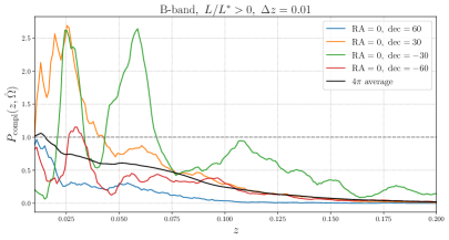
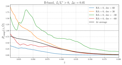
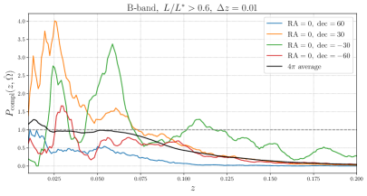
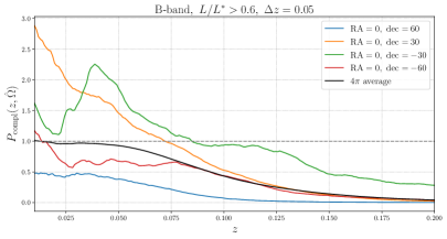
Figure 23: The function $P_{\rm compl}(z,\hat{\Omega})$ with B-band luminosity weighting, for different choices of $\Delta z$ and $L_{\rm cut}$ for four sky directions, and for the $4\pi$ average $P_{\rm compl}(z)$. Upper panels: with no luminosity cut and $\Delta z=0.01$ (left) and $\Delta z=0.05$ (right). Lower panels: the same, restricting to galaxies with $L>0.6L^{*}_{B}$.

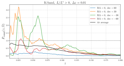
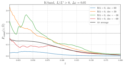
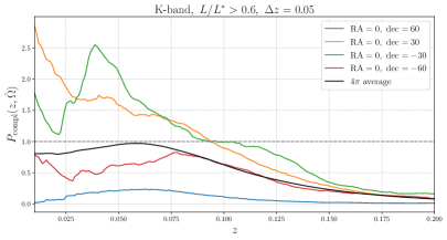
Figure 24: As in Fig. 23, for K band.

All plots on the left panels confirm that the choice $\Delta z=0.01$ is too small, since the actual over- and under-densities are clearly seen, and we do not want to artificially compensate them with the completion. We therefore restrict to the panels with $\Delta z=0.05$. We first observe that, up to some critical $z$, the completeness is larger than one. This over-completeness at small distances is due to local over-densities. These results agree with similar plots shown in refs. [99, 31]. Clearly, it would be meaningless to ‘compensate’ these over-densities by assigning a negative luminosity density that brings back $P_{\rm compl}(z,\hat{\Omega};\Delta z,\Delta\Omega)$ to the ‘expected’ value of one. Then, as already mentioned in sect. 3.2.2, once fixed $\Delta z$ and $\Delta\Omega$, for each direction $\hat{\Omega}$ our strategy will be to look for the highest value of $z$ for which $P_{\rm compl}(z,\hat{\Omega})=1$, that we denote by $z_{*}(\hat{\Omega})$. For $z<z_{*}(\hat{\Omega})$ we will use the galaxy catalog as it is, considering it complete [which formally amounts to setting $P_{\rm compl}(z,\hat{\Omega})=1$ in eqs. (3.58) or (3.70)] while, for $z>z_{*}(\hat{\Omega})$, we will complete the catalog according to the homogeneous completion or to the multiplicative completion discussed in sect. 3.2.2. From the plots in the right panels we see that, in all cases, for $\Delta z=0.05$ and $z>z_{*}(\hat{\Omega})$, $P_{\rm compl}(z,\hat{\Omega})$ is basically a smoothly decreasing function of redshift, and therefore $\Delta z=0.05$ is an adequate choice.

Comparison with Fig. 20 shows that luminosity weighting (both in B band and in K band) improves the completeness dramatically. To understand the best choice for the luminosity cut, in the left panel of Fig. 25 we show the angular average $P_{\rm compl}(z)$ for $\Delta z=0.05$ and several different choices of $L_{\rm cut}$, for B-band. As expected, the completeness increases with the cut. On the other hand, the number of galaxies in the catalog, even if luminosity weighted, decreases as we increase the cut. In the right panel Fig. 25 we show the distribution of B-band luminosities in GLADE, weighting the galaxies by their luminosity (which is the relevant quantity when we use luminosity weighting). The yellow, green and red and dashed vertical lines mark the values $L_{B}=0.3L_{B}^{*}$, $L_{B}=0.6L_{B}^{*}$ and $L_{B}=L_{B}^{*}$, respectively. We see that, raising the cut from $L_{\rm cut}=0$ to $L_{\rm cut}=0.3L_{B}^{*}$, or from $L_{\rm cut}=0.3L_{B}^{*}$ to $L_{\rm cut}=0.6L_{B}^{*}$ we lose a limited fraction of (luminosity-weighted) galaxies, while we have a good increase in completeness; in contrast, passing from $L_{\rm cut}=0.6L_{B}^{*}$ to $L_{\rm cut}=L_{B}^{*}$, we begin to lose a more significant fraction of the integrated luminosity, because we approach the peak of the distribution, while the increase in completeness, especially at large $z$, is not so significant. On this ground, we choose $L_{\rm cut}=0.6L_{B}^{*}$. A rather similar situation takes place for K-band, as we see from Fig. 26, and will choose again $L_{\rm cut}=0.6L_{K}^{*}$.

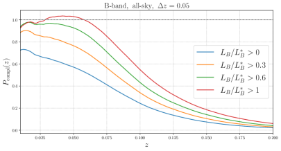
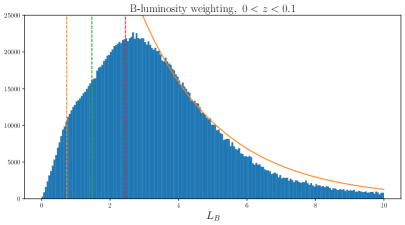
Figure 25: Left: the function $P_{\rm compl}(z)$, for $\Delta z=0.05$ and different luminosity cuts. Right: the number of galaxy per luminosity bin in the GLADE catalog, weighting each galaxy by its luminosity, in B-band. The yellow, green and red and dashed vertical lines mark the values $L_{B}=0.3L_{B}^{*}$, $L_{B}=0.6L_{B}^{*}$ and $L_{B}=L_{B}^{*}$, respectively. The yellow continuous line is the fit to the Schechter function, as in Fig. 22, now in terms of luminosity rather than absolute magnitude.

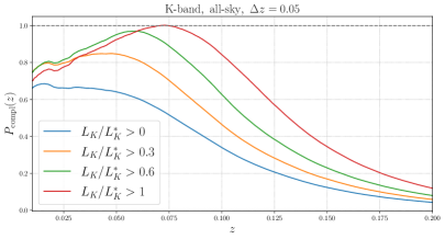
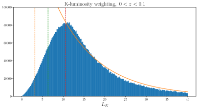
Figure 26: As in Fig. 25, for K band.

To summarize, the results of this appendix indicate that: (1) the use of all galaxies without luminosity weighting, for the GLADE catalog, is not appropriate because of the very limited completeness. We will therefore not use the $w_{\alpha}=1$ weighting for GLADE. (2) B-band and K-band luminosity weighting, with a lower cut on the luminosity, produces a good level of completeness up to redshifts $z\simeq 0.1$ and a still potentially useful level of completeness (i.e., at least larger than $10\%$ in most directions) up to $z\simeq 0.2$. Setting the cut in B band at $L_{\rm cut}=0.6L_{B}^{*}$, and in K band at $L_{\rm cut}=0.6L_{K}^{*}$, appears to be a good compromise between having a sample of galaxies as complete as possible and as large as possible. (3). For the region ${\cal S}$ used to define cone completeness, a good choice is given by a section of a cone, with half-opening angle $\theta_{c}=5^{\circ}$ extending, in the transverse size, between redshifts $z\pm\Delta z/2$ with $\Delta z=0.05$. We will therefore use these choices in our analysis.

A final technical point concerns the treatment of the error on the redshifts of the galaxies. The GLADE catalog does not provide the error on the redshift of the individual galaxies. The simplest option is to assign to all galaxies a gaussian uncertainty $\Delta v\simeq 200\,{\rm km/s}$, corresponding to $\Delta z=\Delta v/c\simeq 6.7\times 10^{-4}$, as in [31, 88]. This reflects a typical value of the peculiar velocities of the galaxies with respect to the Hubble flow. However, in the GLADE catalog the redshifts have already been corrected for peculiar velocities, using an algorithm described in [99]. Thus, what really matters here is the residual error in the measurement of the galaxy redshift, which depends on whether the redshift has been determined spectroscopically or photometrically. In the former case, for the GLADE catalog, $\Delta z$ is dominated by the uncertainty in the correction for peculiar velocities, and can be taken to be $\Delta z\simeq 1.5\times 10^{-4}$, while, for photometric redshifts, this is dominated by the error in the measurement of the redshift, which in this case is typically of order $\Delta z\simeq 1.5\times 10^{-2}$ [99]. The GLADE catalog (v2.4) has a flag that indicates whether the redshift has been obtained photometrically or spectroscopically, so we can assign the corresponding average error to each galaxy. We then use, in eq. (3.29), a gaussian with the variance chosen according to whether the galaxy has a spectroscopic of photometric redshift, using $\Delta z\simeq 1.5\times 10^{-4}$ and redshifts $\Delta z\simeq 1.5\times 10^{-2}$, respectively. We finally convolve the gaussian with a prior given by $p(z)=dV_{c}/dz$, as discussed below eq. (3.29).

Appendix B Dependence of the prior on the region ${\cal R}$

As we saw in sect. 3.2, upon completion the prior can be written in the form (3.35). At this level, it is necessary to specify a region ${\cal R}$ over which we compare the galaxies in the catalog to those that are missing. In this appendix we show that, in the end, the estimate of the parameters such as $H_{0}$ or $\Xi_{0}$ is independent of ${\cal R}$, as long as it is sufficiently larger than the localization region of the ensemble of all GW events (of the type that we are considering in the correlation, e.g. BBH, or BNS) detectable by the GW detector network.

This can be shown directly starting from eq. (3.2). To keep the notation more compact, we write

$$\sum_{\alpha=1}^{N_{\rm gal}({\cal R})}w_{\alpha}\equiv w_{\rm gal}({\cal R})\,,\qquad\sum_{\alpha=1}^{N_{\rm cat}({\cal R})}w_{\alpha}\equiv w_{\rm cat}({\cal R})\,,$$ (B.1)

and we use the shorthand $\delta(z-z_{\alpha})\delta^{(2)}(\hat{\Omega}-\hat{\Omega}_{\alpha})\equiv\delta(x-x_{\alpha})$. We consider for simplicity a single GW event (the argument is trivially generalized) and we take ${\cal R}_{1}$ to be the localization region of the GW event, say at $99.9\%$ c.l., and ${\cal R}_{2}$ a much larger region, that includes ${\cal R}_{1}$. Then

$$p_{0}(x;{\cal R}_{1})=\frac{1}{w_{\rm gal}({\cal R}_{1})}\left[\sum_{\alpha_{1}=1}^{N_{\rm cat}({\cal R}_{1})}w_{\alpha_{1}}\delta(x-x_{\alpha_{1}})+\sum_{\alpha_{2}=1}^{N_{\rm miss}({\cal R}_{1})}w_{\alpha_{2}}\delta(x-x_{\alpha_{2}})\right]\,,$$ (B.2)

$$p_{0}(x;{\cal R}_{2})=\frac{1}{w_{\rm gal}({\cal R}_{2})}\left[\sum_{\alpha_{1}=1}^{N_{\rm cat}({\cal R}_{2})}w_{\alpha_{1}}\delta(x-x_{\alpha_{1}})+\sum_{\alpha_{2}=1}^{N_{\rm miss}({\cal R}_{2})}w_{\alpha_{2}}\delta(x-x_{\alpha_{2}})\right]\,.$$ (B.3)

We now observe that, when in eq. (3.17) we multiply $p_{0}(z,\hat{\Omega};{\cal R}_{2})$ by the GW likelihood $p({\cal D}^{i}_{\rm GW}|z,\hat{\Omega},\theta^{\prime},H_{0})$, all terms in the sums in eq. (B.3) that fall outside the localization region ${\cal R}_{1}$ do not contribute, since there $p({\cal D}^{i}_{\rm GW}|z,\hat{\Omega},H_{0})$ is zero to all practical purposes. Therefore both sums in eq. (B.3) are effectively restricted to the region ${\cal R}_{1}$ and, in eq. (3.17), to use $p_{0}(x;{\cal R}_{2})$ is the same as using a prior $\tilde{p}_{0}(x;{\cal R}_{2})$ given by

$$\tilde{p}_{0}(x;{\cal R}_{2}) = \frac{1}{w_{\rm gal}({\cal R}_{2})}\left[\sum_{\alpha_{1}=1}^{N_{\rm cat}({\cal R}_{1})}w_{\alpha_{1}}\delta(x-x_{\alpha_{1}})+\sum_{\alpha_{2}=1}^{N_{\rm miss}({\cal R}_{1})}w_{\alpha_{2}}\delta(x-x_{\alpha_{2}})\right]$$ (B.4)

$$= \frac{w_{\rm gal}({\cal R}_{1})}{w_{\rm gal}({\cal R}_{2})}\,p_{0}(x;{\cal R}_{1})\,.$$

The overall constant $w_{\rm gal}({\cal R}_{1})/w_{\rm gal}({\cal R}_{2})$ cancels between numerator and denominator in eq. (3.17), with the denominator given by eq. (3.23). Therefore, in the end, while it is necessary to introduce a region ${\cal R}$ so that the expressions in eqs. (3.31)–(3.36) are well defined, its exact definition is irrelevant, as long as it covers the localization region of the GW event.

Appendix C Semi-analytic evaluation of $\beta$ including the distribution of source parameters

In this appendix we discuss an approach to the computation of $\beta(H_{0})$ and $\beta(\Xi_{0})$, that allows us to include the effect of the distribution of source parameters, with a relatively simple semi-analytic technique. We stress that, for producing our final results, we have used only our MC computation of $\beta$ (to be briefly discussed in app. D). However, the semi-analytic computation that we discuss here provides simple and ready to use formulas, a physical understanding of some effects, and a check for the MC itself, so we find useful to present it here.

We will limit ourselves to the distribution of component masses and orbit inclination, although the technique could in principle be generalized to other parameters. For the orbit inclination we assume a uniform prior for the source population. We keep for the moment generic the distribution of masses for the BH-BH population, and we denote it as $\tilde{p}_{0}(m_{1},m_{2})$. We will later specify it to the broken power-law distribution (3.102) proposed in [6].

To compute the SNR, for this simple semi-analytic estimate we work in the approximation in which one includes only the inspiral part of waveform, and to lowest-order in the post-Newtonian expansion. As discussed in [133, 134], the result of the actual detection pipelines is well approximated by the criterion that the SNR in the second loudest detector is larger than 8. For O2, we checked this assumption by computing the selection effects with ${\rm SNR}>8$ using inspiral-only waveforms, and comparing with publicly available LVC injections (we use the data in the file injections_O1O2an_spin.h5 at https://dcc.ligo.org/LIGO-P2000434-v1/public), and we found good agreement. For O3, this becomes a poorer approximation because of the heavier BBH masses of many events, which implies that these signals stay in the bandwidth for a small number of inspiral cycles. For this reason, our final results are obtained with a MC, where we have used exclusively full inspiral-merger-ringdown waveforms, both for O1-O2 and for O3a data. The semi-analytic technique that we are discussing could, in principle, be generalized beyond the inspiral waveform, but, in any case, our aim here is simply to improve on the analytic understanding provided by the lowest-order computation in presented in [15, 31].

In the approximation in which only the inspiral part of the waveform is included, the SNR in a single detector is given by [135] (see, e.g., sects. 4.1.4 and 7.7.2 of [49] for review)

$$({\rm SNR})^{2}=\frac{5}{6}\frac{(G{\cal M}_{c})^{5/3}|Q(\cos\iota,\hat{\Omega})|^{2}}{c^{3}\pi^{4/3}d_{L}^{2}}\,I_{7/3}({\cal M}_{\rm tot})\,,$$ (C.1)

where

$$I_{7/3}({\cal M}_{\rm tot})\equiv\int_{f_{\mathrm{min}}}^{f_{\rm insp}(z)}df\,\frac{f^{-7/3}}{S_{n}(f)}\,,$$ (C.2)

and ${\cal M}_{c}(z)=(1+z)M_{c}$ and ${\cal M}_{\rm tot}(z)=(1+z)M_{\rm tot}$ are the redshifted (‘detector-frame’) chirp mass and total mass of the system, respectively [with $M_{c}=(m_{1}m_{2})^{3/5}/M_{\rm tot}^{1/5}$ and $M_{\rm tot}=m_{1}+m_{2}$]; the factor

$$|Q(\cos\iota,\hat{\Omega})|^{2}=F_{+}^{2}(\hat{\Omega})\,\left(\frac{1+\cos^{2}\iota}{2}\right)^{2}+F_{\times}^{2}(\hat{\Omega})\cos^{2}\iota\,,$$ (C.3)

[where $F_{+,\times}(\hat{\Omega})$ are the pattern functions of the interferometer] encodes the detector response to the inclination angle $\iota$ of the orbit and to the source direction; $S_{n}(f)$ is the noise spectral density of the detector; $f_{\min}$ is the low frequency limit of the detector bandwidth, and $f_{\mathrm{insp}}(z)=f_{\mathrm{insp}}/(1+z)$ is the observed (redshifted) gravitational-wave frequency at the end of the inspiral phase. In the approximation in which we only consider the contribution to the SNR from the inspiral, the latter can be approximated as twice the orbital frequency at the innermost stable circular orbit, which gives $f_{\mathrm{insp}}\simeq 4.4\,{\rm kHz}\,(M_{\odot}/M_{\rm tot})$ [49], so in the end

$$f_{\mathrm{insp}}(z)\simeq 4.4\,{\rm kHz}\,\frac{M_{\odot}}{{\cal M}_{\rm tot}(z)}\,.$$ (C.4)

Including higher orders in the PN expansion, as well as the part of the waveform describing merger and ringdown, brings in the dependence on other parameters, such as the BH spins. Note that, in the context of modified gravity, in eq. (C.1) $d_{L}$ must be replaced by the GW luminosity distance $d_{L}^{\,\rm gw}$.

To evaluate eq. (C.2) we use an expression for $S_{h}(f)$ typical of the detectors at the time of detection. This changes between runs, such as the O2 and O3 run, and therefore also the the beta functions depends on the run considered. As detection criterion, we set a threshold value ${\rm SNR}_{t}=8$. In practice, the searches employed by LIGO/Virgo rather use a threshold on the false alarm rate of the detector network to identify the detections. However, at least at the level of O2 data, in terms of SNR this search is well approximated by the condition that the threshold in the inspiral SNR of the second-most-sensitive detector is greater than 8 [133, 134].

Adding to the list of $\theta^{\prime}$ parameters in eq. (3.23) the two BH source-frame masses $m_{1}$ and $m_{2}$ (with $m_{1}\geq m_{2}$) and the inclination angle $\iota$, eq. (3.79) is replaced by

$$\beta(H_{0}) = \int_{0}^{z_{\cal R}}dz\int d\Omega\,p_{0}(z,\hat{\Omega})\int dm_{1}dm_{2}\,\tilde{p}_{0}(m_{1},m_{2})\,$$ (C.5)

$$\times\int_{-1}^{1}\frac{d\cos\iota}{2}\,P_{\rm det}\left[d_{L}(z,H_{0}),\hat{\Omega},\cos\iota,{\cal M}_{1}(z),{\cal M}_{2}(z)\right]\,,$$

where $\tilde{p}_{0}(m_{1},m_{2})$ is the normalized distribution of BH masses, and ${\cal M}_{1,2}(z)=(1+z)m_{1,2}$ are the corresponding detector-frame masses. Notice that, according to eq. (C.1) (as well as to its generalization beyond the lowest-order inspiral), the SNR, and therefore the detection probability, is a function of the detector-frame masses, rather than of the source-frame masses, while the distribution probability for the BH masses is at first more naturally expressed in terms of the intrinsic, source-frame, masses. The distribution in the inclination angle has been taken flat in $\cos\iota$, and the factor $1/2$ normalizes it to one. For definiteness, we illustrate the procedure for $\beta(H_{0})$ but all the results below are trivially adapted to the case of $\beta(\Xi_{0})$.

We begin by evaluating this expression for the homogeneous completion, when $p_{0}(z,\hat{\Omega})$ is given by eq. (3.65). The result can be written as

$$\beta^{\rm hom}(H_{0})=\beta_{\rm cat}(H_{0})+\beta_{\rm compl}(H_{0})\,,$$ (C.6)

where $\beta_{\rm cat}(H_{0})$ is the term that depends on the catalog, while the term $\beta_{\rm compl}(H_{0})$ reflects the homogeneous component added by the completion procedure. The former is given by

$$\beta_{\rm cat}(H_{0})=\left(\frac{\int_{0}^{z_{\cal R}}dz^{\prime}\,j(z^{\prime})P_{\rm compl}(z^{\prime})}{\int_{0}^{z_{\cal R}}dz^{\prime}\,j(z^{\prime})}\right)\,\frac{\sum_{\alpha=1}^{N_{\rm cat}({\cal R})}w_{\alpha}\beta_{\alpha}(H_{0})}{\sum_{\alpha=1}^{N_{\rm cat}({\cal R})}w_{\alpha}}\,,$$ (C.7)

where

$$\beta_{\alpha}(H_{0})=\int dm_{1}dm_{2}\,\tilde{p}_{0}(m_{1},m_{2})\,\int_{-1}^{1}\frac{d\cos\iota}{2}\,P_{\rm det}\left[d_{L}(z_{\alpha},H_{0}),\hat{\Omega}_{\alpha},\cos\iota,{\cal M}_{1}(z_{\alpha}),{\cal M}_{2}(z_{\alpha})\right]\,.$$ (C.8)

The term $\beta_{\rm compl}(H_{0})$ is given

$$\beta_{\rm compl}(H_{0}) = \frac{1}{4\pi\int_{0}^{z_{\cal R}}dz^{\prime}\,j(z^{\prime})}\,\int_{0}^{z_{\cal R}}dz\,j(z)\int d\Omega\,\left[1-P_{\rm compl}(z,\hat{\Omega})\right]$$

$$\times\int dm_{1}dm_{2}\,\tilde{p}_{0}(m_{1},m_{2})\int_{-1}^{1}\frac{d\cos\iota}{2}\,P_{\rm det}\left[d_{L}(z,H_{0}),\hat{\Omega},\cos\iota,{\cal M}_{1}(z),{\cal M}_{2}(z)\right]\,.$$

In the semi-analytic approach, a significant simplification can be obtained approximating $P_{\rm det}$ by its average over the solid angle. This can be justified observing that the orientation of a given galaxy with respect to the interferometer arms changes with the Earth rotation. Adding to the list of $\theta^{\prime}$ parameters the time of the day at which the GW signal from a source in a given galaxy arrives, with a uniform prior over 24h, is equivalent to performing, for each galaxy, an angular average over a great circle in the sky. To a first approximation, especially when we are interested in an ensemble of sources, this can be replaced by an angular average over the full sphere. To compute the angular average of $P_{\rm det}$ we take the angular average of eq. (C.1). For interferometers, the angular average over $\hat{\Omega}$ gives $\langle F_{+}^{2}(\hat{\Omega})\rangle=\langle F_{\times}^{2}(\hat{\Omega})\rangle=1/5$, so $\langle|Q(\cos\iota,\hat{\Omega})|^{2}\rangle=(1/5)g(\cos\iota)$, where

$$g(\cos\iota)=\left(\frac{1+\cos^{2}\iota}{2}\right)^{2}+\cos^{2}\iota\,,$$ (C.10)

and eq. (C.1) becomes

$${\rm SNR}^{2}(d_{L},\cos\iota,{\cal M}_{1},{\cal M}_{2})=g(\cos\iota)\,\frac{(G{\cal M}_{c})^{5/3}}{6\pi^{4/3}c^{3}d_{L}^{2}}\,I_{7/3}({\cal M}_{\rm tot})\,.$$ (C.11)

We set a threshold value ${\rm SNR}_{t}$ in the signal-to-noise ratio as a criterion for detection, and we observe that the average of $g(\iota)$ over $\cos\iota$ is equal to $4/5$. This motivates the definition of $d_{H}({\cal M}_{1},{\cal M}_{2})$, given by (see e.g. eq. (7.182) of [49])

$${\rm SNR}_{t}^{2}=\frac{4}{5}\,\frac{(G{\cal M}_{c})^{5/3}}{6\pi^{4/3}c^{3}d_{H}^{2}({\cal M}_{1},{\cal M}_{2})}\,I_{7/3}({\cal M}_{\rm tot})\,.$$ (C.12)

The physical meaning of $d_{H}({\cal M}_{1},{\cal M}_{2})$ is that it is the distance at which a compact binary with (detector-frame) masses ${\cal M}_{1},{\cal M}_{2}$ can be detected, in a single interferometer, with a threshold ${\rm SNR}_{t}$ in the signal-to-noise ratio, after averaging over direction and inclination (this quantity is usually called the ‘range’ to the compact binary in question). In terms of $d_{H}({\cal M}_{1},{\cal M}_{2})$, eq. (C.11) can be rewritten more compactly as

$${\rm SNR}(d_{L},\cos\iota,{\cal M}_{1},{\cal M}_{2})={\rm SNR}_{t}\,\left(\frac{g(\cos\iota)}{4/5}\right)^{1/2}\,\frac{d_{H}({\cal M}_{1},{\cal M}_{2})}{d_{L}}\,.$$ (C.13)

For a generic ${\rm SNR}_{t}$, with our detection criterion we have

$$P_{\rm det}(d_{L},\cos\iota,{\cal M}_{1},{\cal M}_{2})=\theta\left[{\rm SNR}(d_{L},\cos\iota,{\cal M}_{1},{\cal M}_{2})-{\rm SNR}_{t}\right]\,,$$ (C.14)

which, using eq. (C.13), can be rewritten as

$$P_{\rm det}(d_{L},\cos\iota,{\cal M}_{1},{\cal M}_{2})=\theta\left[g(\cos\iota)-\frac{4}{5}\,\frac{d^{2}_{L}}{d^{2}_{H}({\cal M}_{1},{\cal M}_{2})}\right]\,.$$ (C.15)

In the following we will set ${\rm SNR}_{t}=8$ and therefore, from eq. (C.12),

$$d_{H}({\cal M}_{1},{\cal M}_{2})=\frac{1}{20}\,\left(\frac{5}{6}\right)^{1/2}\,\frac{1}{\pi^{2/3}c^{3/2}}\,(G{\cal M}_{c})^{5/6}I_{7/3}^{1/2}({\cal M}_{\rm tot})\,.$$ (C.16)

Having dropped the dependence of $P_{\rm det}$ on $\hat{\Omega}$, eq. (C.8) simplifies to

$$\beta_{\alpha}(H_{0})=\int dm_{1}dm_{2}\,\tilde{p}_{0}(m_{1},m_{2})\,\int_{0}^{1}d\cos\iota\,P_{\rm det}\left[d_{L}(z_{\alpha},H_{0}),\cos\iota,{\cal M}_{1}(z_{\alpha}),{\cal M}_{2}(z_{\alpha})\right]\,.$$ (C.17)

(Note that, since $g(\cos\iota)$ is even under $\cos\iota\rightarrow-\cos\iota$, the integral over $\cos\iota$ from $-1$ to $1$ becomes twice the integral from 0 to 1.) Similarly, dropping the dependence of $P_{\rm det}$ on $\hat{\Omega}$, the term $\beta_{\rm compl}(H_{0})$ in eq. (C) simplifies to

$$\beta_{\rm compl}(H_{0}) = \frac{1}{\int_{0}^{z_{\cal R}}dz^{\prime}\,j(z^{\prime})}\,\int_{0}^{z_{\cal R}}dz\,j(z)\,\left[1-P_{\rm compl}(z)\right]$$

$$\times\int dm_{1}dm_{2}\,\tilde{p}_{0}(m_{1},m_{2})\int_{0}^{1}d\cos\iota\,P_{\rm det}\left[d_{L}(z,H_{0}),\cos\iota,{\cal M}_{1}(z),{\cal M}_{2}(z)\right]\,.$$

It is convenient to express also the mass distribution function in terms of the detector-frame masses, defining $\tilde{p}({\cal M}_{1},{\cal M}_{2};z)$ from

$$dm_{1}dm_{2}\,\tilde{p}_{0}(m_{1},m_{2})=d{\cal M}_{1}d{\cal M}_{2}\,\tilde{p}({\cal M}_{1},{\cal M}_{2};z)\,,$$ (C.19)

Using eqs. (C.10) and (C.15), the integration over $\cos\iota$ in eqs. (C.17) and (C) can be done explicitly. Observing that $g(\cos\iota)$ is a monotonically increasing function of $\cos\iota$, such that $g(0)=1/4$ and $g(1)=2$, we see that the theta function in eq. (C.15) is always satisfied if $(4/5)d_{L}^{2}/d_{H}^{2}<1/4$, in which case the integral over $\cos\iota$ is equal to one, and is never satisfied if $(4/5)d_{L}^{2}/d_{H}^{2}>2$. In the intermediate regime there is one value $\cos\iota_{*}$ such that $g(\cos\iota_{*})=(4/5)d_{L}^{2}/d_{H}^{2}$, and the integral is equal to $1-\cos\iota_{*}$. In this way we get

$$\int_{0}^{1}d\cos\iota\,P_{\rm det}\left[d_{L},\cos\iota,{\cal M}_{1}(z),{\cal M}_{2}(z)\right]=f\left(\frac{4}{5}\,\frac{d^{2}_{L}}{d^{2}_{H}({\cal M}_{1},{\cal M}_{2})}\right)\,,$$ (C.20)

where

$$f(x)\equiv\left\{\begin{array}[]{lcc}1&\quad{\rm for}&\quad x\leq 1/4\\ 1-\sqrt{2\sqrt{x+2}-3}&\quad{\rm for}&\quad 1/4\leq x\leq 2\\ 0&\quad{\rm for}&\quad x\geq 2\,.\\ \end{array}\right.$$ (C.21)

It is convenient to define the function

$$B(d_{L};z)\equiv\int d{\cal M}_{1}d{\cal M}_{2}\,\tilde{p}({\cal M}_{1},{\cal M}_{2};z)\,f\left(\frac{4}{5}\,\frac{d^{2}_{L}}{d^{2}_{H}({\cal M}_{1},{\cal M}_{2})}\right)\,.$$ (C.22)

Note that $B(d_{L};z)$ depends both on $d_{L}$, which is itself a function of $z$ and $H_{0}$, and also explicitly on $z$ because of the dependence on $z$ in $\tilde{p}({\cal M}_{1},{\cal M}_{2};z)$. The latter enters only through the $z$ dependence of ${\cal M}_{\rm min}(z)=(1+z)m_{\rm min}$ and ${\cal M}_{\rm max}(z)=(1+z)m_{\rm max}$.

Then putting everything together, for homogeneous completion

$$\beta(H_{0}) = \left(\frac{\int_{0}^{z_{\cal R}}dz^{\prime}\,j(z^{\prime})P_{\rm compl}(z^{\prime})}{\int_{0}^{z_{\cal R}}dz^{\prime}\,j(z^{\prime})}\right)\,\frac{\sum_{\alpha=1}^{N_{\rm cat}({\cal R})}w_{\alpha}B[d_{L}(z_{\alpha},H_{0});z_{\alpha}]}{\sum_{\alpha=1}^{N_{\rm cat}({\cal R})}w_{\alpha}}$$ (C.23)

$$+\frac{1}{\int_{0}^{z_{\cal R}}dz^{\prime}\,j(z^{\prime})}\,\int_{0}^{z_{\cal R}}dz\,j(z)\,\left[1-P_{\rm compl}(z)\right]\,B[d_{L}(z,H_{0});z]\,.$$

Comparing with eq. (3.92) we see that the function $B[d_{L}(z,H_{0});z]$ plays the role of a smooth cutoff function, that replaces the theta function $\theta[z_{\rm max}(H_{0};d_{\rm max})-z]$, with $z_{\max}(H_{0})$ determined by $d_{L}(z_{\rm max};H_{0})=d_{\rm max}$, that was coming from the simplified detection model, and that would become quite arbitrary for a population of sources, for which there is no single notion of maximum detection distance. Similarly, eq. (3.96) is replaced by

$$\beta(\Xi_{0}) = \left(\frac{\int_{0}^{z_{\cal R}}dz^{\prime}\,j(z^{\prime})P_{\rm compl}(z^{\prime})}{\int_{0}^{z_{\cal R}}dz^{\prime}\,j(z^{\prime})}\right)\,\frac{\sum_{\alpha=1}^{N_{\rm cat}({\cal R})}w_{\alpha}B[d_{L}^{\,\rm gw}(z_{\alpha},\Xi_{0});z_{\alpha}]}{\sum_{\alpha=1}^{N_{\rm cat}({\cal R})}w_{\alpha}}$$ (C.24)

$$+\frac{1}{\int_{0}^{z_{\cal R}}dz^{\prime}\,j(z^{\prime})}\,\int_{0}^{z_{\cal R}}dz\,j(z)\,\left[1-P_{\rm compl}(z)\right]\,B[d_{L}^{\,\rm gw}(z,\Xi_{0});z]\,,$$

with $d_{L}^{\,\rm gw}(z,\Xi_{0})$ replacing $d_{L}(z,H_{0})\equiv d_{L}^{\,\rm em}(z,H_{0})$ in the argument of $B(d_{L})$ (and, as usual, we have not written explicitly the dependence of $d_{L}^{\,\rm gw}$ on $H_{0}$ when we study $\Xi_{0}$).

It is straightforward to repeat this computation for multiplicative completion. The results are

$$\beta^{\rm multi}(H_{0})=\left(\frac{\int_{0}^{z_{\cal R}}dz^{\prime}\,j(z^{\prime})P_{\rm compl}(z^{\prime})}{\int_{0}^{z_{\cal R}}dz^{\prime}\,j(z^{\prime})}\right)\,\frac{\sum_{\alpha=1}^{N_{\rm cat}({\cal R})}w_{\alpha}B[d_{L}(z_{\alpha},H_{0});z_{\alpha}]/P_{\alpha}}{\sum_{\alpha=1}^{N_{\rm cat}({\cal R})}w_{\alpha}}\,,$$ (C.25)

and

$$\beta^{\rm multi}(\Xi_{0})=\left(\frac{\int_{0}^{z_{\cal R}}dz^{\prime}\,j(z^{\prime})P_{\rm compl}(z^{\prime})}{\int_{0}^{z_{\cal R}}dz^{\prime}\,j(z^{\prime})}\right)\,\frac{\sum_{\alpha=1}^{N_{\rm cat}({\cal R})}w_{\alpha}B[d_{L}^{\,\rm gw}(z_{\alpha},\Xi_{0});z_{\alpha}]/P_{\alpha}}{\sum_{\alpha=1}^{N_{\rm cat}({\cal R})}w_{\alpha}}\,,$$ (C.26)

which generalize eq. (3.97) and the corresponding result for $\beta(\Xi_{0})$, again with $B[d_{L}(z,H_{0});z]$ or $B[d_{L}^{\,\rm gw}(z,\Xi_{0});z]$, respectively, replacing the theta functions. The same therefore happens for the mixture of homogeneous and multiplicative completion discussed in the text, and for the extention to $\lambda\neq 1$ discussed in eqs. (3.114)–(3.117).

Observe that the above results, that have been obtained using just the expression for the SNR with the lowest-order inspiral waveform, can be generalized to more accurate computations of the waveform. Indeed, as long as we work within the so-called restricted post-Newtonian (PN) approximation, where one considers corrections to the phase of the waveform of a coalescing binaries, but keeps only the lowest order in the amplitude, the dependence of the SNR on $\cos\iota$ remains the one that we have used, and therefore the integration over $\cos\iota$ goes through in the same way (in contrast, going beyond the restricted PN approximation the dependence on $\cos\iota$ changes, see sect. 5.6.4 of [49]). Then, in the above results we can simply replace the horizon distance $d_{H}({\cal M}_{1},{\cal M}_{2})$, that in our lowest-order inspiral-only approximation is given by eq. (C.16), with the expression obtained from the waveform used. If the latter includes the spins of the compact bodies (or other variables such as eccentricity. etc.), these variables must then be added to the list of integration variables in eq. (C.22).

We now evaluate these expression for the choice (3.102) of mass distribution. The function $B(d_{L};z)$ can be computed by direct numerical evaluation of the double integral in eq. (C.22). The left panel of Fig. 4, on page 4 of the main text, shows the result for $B(d_{L})\equiv B[d_{L};z(d_{L},H_{0})]$, using the O2 strain sensitivity to compute the integral $I_{7/3}({\cal M}_{\rm tot})$ that enters in eq. (C.16), for a population of BBHs, using the reference values (3.103), (3.104) in the mass distribution (3.102), and setting $H_{0}=70\,\,{\rm km}\,{\rm s}^{-1}\,{\rm Mpc}^{-1}$. First of all we see that, for $d_{L}$ smaller than a value $d_{0}$, $B(d_{L})=1$. This is easily understood: with the mass distribution that we are using, the BBH which has the lowest SNR, for a given distance, is the lightest system in our distribution, $m_{1}=m_{2}=2.2M_{\odot}$, when it has the most unfavorable orientation, $\cos\iota=0$, so that $g(\cos\iota)$ attains its its minimum value of $1/4$. When $d_{L}$ is so small that even this system goes above the detection threshold, all the BBHs in our distribution are above threshold, so the function $f(x)$ in eq. (C.21) is always equal to one, and then also $B(d_{L})=1$, since the mass distribution is normalized to one. From eq. (C.15), the value of $d_{0}$ is therefore given by

$$d_{0}=\frac{\sqrt{5}}{4}\,d_{H}(2.2M_{\odot},2.2M_{\odot})\,,$$ (C.27)

which, using the O2 strain sensitivity to compute $d_{H}(m_{1},m_{2})$, gives $d_{0}\simeq 71.69\,{\rm Mpc}$. Above this value, we find that the numerical result is very well fitted by an exponential with a linear and a quadratic term in $(d_{L}-d_{0})$. Therefore

$$B(d_{L})=1\,,\qquad(d_{L}\leq d_{0})\,,$$ (C.28)

and

$$B(d_{L})\simeq e^{-a_{0}\frac{d_{L}-d_{0}}{d_{0}}-a_{1}\left(\frac{d_{L}-d_{0}}{d_{0}}\right)^{2}}\,,\qquad(d_{L}>d_{0})\,.$$ (C.29)

Using $\gamma_{1}=1.05$ in the mass distribution (3.102) for BBHs, together with the other reference values given in eqs. (3.103) and (3.104), and the best O2 sensitivity curve (see footnote 61) the fit gives $a_{0}\simeq 0.215$, $a_{1}\simeq 0.004$. Similar considerations hold for the right panel of Fig. 4, that shows the corresponding result for a BNS population with a distribution for the source-frame masses flat in the range $[1-3]M_{\odot}$. In this case, the fit gives $a_{0}\simeq 0.106$, $a_{1}\simeq 0.144$, and the corresponding value of $d_{0}$ is $d_{0}=(\sqrt{5}/4)d_{H}(M_{\odot},M_{\odot})\simeq 37.2\,{\rm Mpc}$. Fig. 4 nicely shows how the naive theta function (3.85) is modified when we deal with a population of BBHs with an extended mass distribution, rather than a monochromatic population.

Notice that, in principle, $B$ is a function of two independent variables, that can be taken to be $d_{L}$ and $z$; alternatively, using the relation $d_{L}=d_{L}(H_{0},z)$, it can be taken to be a function of $z$ and $H_{0}$, or of $d_{L}$ and $H_{0}$. One might then be worried that we should compute it numerically on a two-dimensional grid, for instance in $d_{L}$ and $H_{0}$ (while Fig. 4 was obtained computing it as a function of $d_{L}$, at fixed $H_{0}$). Fortunately, this is not the case and, when using $d_{L}$ and $H_{0}$ as independent variables, $B(d_{L},H_{0})$ is basically independent of $H_{0}$. This is shown in the upper left panel of Fig. 27 where, even taking a very broad range of values of $H_{0}$, the three curves shown are basically indistinguishable. Thus $B(d_{L},H_{0})$ can be extremely well approximated by a function of $d_{L}$ only, with no explicit dependence on $H_{0}$, and given by eqs. (C.28) and (C.29). When we insert it into eqs. (C.23)–(C.26) we need to write it as a function of $z$, to compare with the redshifts of the galaxies, and this is done writing $d_{L}=d_{L}(z,H_{0})$, so in those equations $B[d_{L}(z,H_{0});z]$ can be simply written as $B[d_{L}(z,H_{0})]$, with no further explicit dependence on $z$, and with $B(d_{L})$ approximated by eqs. (C.28) and (C.29). Then eqs. (C.23)–(C.26) simplify to eqs. (3.106) and (3.107) of the main text.

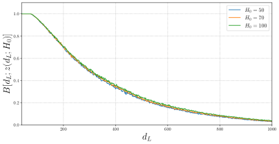
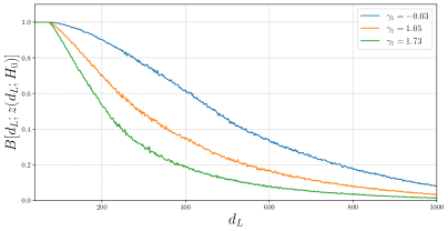
Figure 27: Left panel: the function $B[d_{L};z(d_{L},H_{0})]$, as a function of $d_{L}$, for three different values of $H_{0}$ (in units of ${\rm km}\,{\rm s}^{-1}\,{\rm Mpc}^{-1}$), and the value given in eqs. (3.103) and (3.104) for the other parameters. The three curves are basically indistinguishable. Right panel: the result for different values of $\gamma_{1}$, with the other parameters fixed.

Once computed $B(d_{L})$, the corresponding numerical results for $\beta(H_{0})$ or $\beta(\Xi_{0})$ can be obtained immediately from a numerical evaluation of eq. (C.23) or eq. (C.25). These results then allow us to compute a first approximation to $\beta(H_{0})$ or $\beta(\Xi_{0})$, including the mass distribution, and can be used to estimate the dependence of the result on the choice of parameters, such as $\gamma_{1}$, without the need of performing each time an MC. Actually, we found that the limit $P_{\rm compl}(z)=0$ of eq. (3.106), given by the simple expression

$$\left.\beta^{\rm hom}(H_{0})\right|_{P_{\rm compl}=0}=\frac{\int_{0}^{z_{\cal R}}dz\,j(z)\,\,B[d_{L}(z,H_{0})]}{\int_{0}^{z_{\cal R}}dz^{\prime}\,j(z^{\prime})}\,,$$ (C.30)

is already accurate to better than $5\%$ compared to a MC computation that also employs only the inspiral waveform (and without selection effect on the completeness of the events) over the most relevant range of values of $H_{0}$, and is much faster to compute. However, when selection effects are important, an accurate evaluation of $\beta(H_{0})$ requires a MC computation. Furthermore, the use of full inspiral-merger-waveform is also essential, particularly at the level of O3 data. Therefore, while the above expressions give some useful insight, for instance showing how the theta function is replaced by a smoothed cutoff function $B(d_{L})$ and how the latter is related to the mass distribution, eventually accurate numerical work still requires an MC evaluation, and all the resukts that we present are obtained with such a MC.

Appendix D Monte Carlo evaluation of $\beta(H_{0})$ and $\beta(\Xi_{0})$

In this appendix we give a short description of our MC evaluation of $\beta(H_{0})$ and $\beta(\Xi_{0})$, which is part of our code, publicly available at https://github.com/CosmoStatGW/DarkSirensStat.

For each value of $H_{0}$ (or $\Xi_{0}$) we generate a random sample of merger events by drawing the two source frame masses, inclination angle and detection time (which is used to evaluate the orientation in space of the arms of the interferometers), as well as the position in redshift space. For the latter, we split the computation with our completed galaxy catalog prior into two separate MC integrations as follows. For the part of the prior that depends directly on the galaxy positions in the catalog, we sample galaxies from the luminosity weighted catalog by drawing from the discrete distribution $w^{\text{gal}}_{\alpha}/\sum_{\alpha}w^{\text{gal}}_{\alpha}$ where $w^{\text{gal}}_{\alpha}=w_{\alpha}(1+z_{\alpha})^{\lambda-1}$, and each $z_{\alpha}$ in turn has been sampled from the galaxy posterior of the galaxy denoted by $\alpha$. For the homogenous part that is added to complete the catalog, we importance sample the redshift from $dV_{c}/dz(1+z)^{\lambda-1}/\mathcal{N}(z_{\text{max}})$ up to the maximal detector visibility $z_{\text{max}}$ for the current cosmological parameters at optimal detector-frame masses, where $\mathcal{N}(z_{\text{max}})=\int_{0}^{z_{\text{max}}}(dV_{c}/dz)(1+z)^{\lambda-1}dz$. We then discard all generated GW events that do not satisfy the completeness threshold cut. For the remaining events we evaluate the corresponding completeness factors that appear in our prior, and store them as weights $W_{i}$, where the index $i$ labels the GW event. We then compute, for each event, the theoretical SNR with the PyCBC software and the IMRPhenomXAS waveform model [107], and multiply the weights $W_{i}$ by the probability of detection, assuming a gaussian distribution for the detection SNR, and a detection threshold of 8 in the less loud detector among LIGO Hanford and LIGO Livingston (with their position on Earth at observation time taken into account). The $W_{i}$ for the galaxy term and for the completion term are then multiplied by the factors $\sum_{\alpha}w^{\text{gal}}_{\alpha}$ and $\mathcal{N}(z_{\text{max}})$, respectively, that compensate for the same factors implicitly present at the denominator, due to the fact that the MC samples from normalized distributions. We also need to include factors reflecting the two sample sizes used for the galaxy term and for the completion term, respectively, which we adapt to an estimate of their expected relative sizes to reduce variance of the estimator. Finally, the value of $\beta$ is proportional to the sum of the resulting weights $W_{i}$. This results in an unbiased estimator of $\beta$ at a single value of $H_{0}$ (or $\Xi_{0}$). We repeat this for $\mathcal{O}(1000)$ values of $H_{0}$ (or $\Xi_{0}$), resulting in total to the use of $\mathcal{O}(10^{8})$ sampled events, and we finally filter the resulting function to create a smoother result.

Appendix E Dependence of the results on different choices

In this appendix we discuss how our results change when making different choices with respect to our baseline model that, as discussed in sect. 4, is defined by the fact of using mask completion to quantify the quasi-local completeness level of the catalog, multiplicative completion to fill in the missing galaxies, K-band luminosity weighting, and a completeness threshold $P_{\rm th}=0.7$ for the selection of the GW events.

E.1 Dependence on the completeness threshold

We begin by studying the effect of the completeness threshold $P_{\rm th}$. This choice is determined by a balance between two different considerations. Lowering $P_{\rm th}$ we include more events, and we therefore have a larger statistical sample. On the other hand, when we correlate a GW event with a galaxy catalog, if the GW event falls in a region where the galaxy catalog is very incomplete, the result is eventually dominated by the completion procedure. As we have discussed, see in particular the discussion on page 28 and footnote 28, as long as we know the ‘exact’ functions $\beta(H_{0})$ appropriate to the completion procedure used, events that falls into very incomplete region should give, on average (i.e, after averaging over many such low-completeness events), a flat contribution to the posterior. However, this comes from a delicate compensation of potentially large effects between the numerator and the denominator of the posterior (3.11), and would require a very tight control over the function $\beta(H_{0})$ [or $\beta(\Xi_{0})$], including the precise BBH mass function, details of the detector sensitivities at time of detection, etc. Any error in the computation of $\beta(H_{0})$ or $\beta(\Xi_{0})$ would then systematically bias the contribution from events coming from incomplete regions.

To minimize such systematic biases, a conservative choice is to increase the value of the threshold $P_{\rm th}$, which makes the results less sensitive to the completion procedure, at the price of reducing the statistical sample. The determination of the optimal range of values of $P_{\rm th}$ cannot be made a priori, and requires some experimentation. Here we can be guided by the fact that, even if, in sect. 4.1, for $H_{0}$ we use a very broad prior, $H_{0}\in[30,140]\,\,{\rm km}\,{\rm s}^{-1}\,{\rm Mpc}^{-1}$, we actually know from cosmological observations that the prior range could be significantly restricted. For instance, any peak at $H_{0}\sim 40\,\,{\rm km}\,{\rm s}^{-1}\,{\rm Mpc}^{-1}$ should clearly be spurious. If such a peak happens to disappear increasing $P_{\rm th}$, it is natural to suspect that this spurious peak is due to a partially incorrect completion procedure. We will use this information to obtain some understanding on the optimal choice of $P_{\rm th}$, and we will then use the same value of $P_{\rm th}$ also in the study of $\Xi_{0}$, for which the prior information is less stringent.

Fig. 28 shows the posterior of $H_{0}$ for $P_{\rm th}=0.2$ (left) and $P_{\rm th}=0.5$ (right), while the result for $P_{\rm th}=0.7$ was shown in Fig. 6 on page 6 of the main text. Comparing these three plots, we note first of all that the dependence on $P_{\rm th}$ is very significant. We see that, in the total O1+O2+O3a posterior, for $P_{\rm th}=0.2$ there are two comparable peaks, one at $H_{0}\sim 40\,\,{\rm km}\,{\rm s}^{-1}\,{\rm Mpc}^{-1}$, and one at $H_{0}\sim 70\,\,{\rm km}\,{\rm s}^{-1}\,{\rm Mpc}^{-1}$, where we know that the correct result should be. Both the O1+O2 and the O3a posterior separately show a peak at $H_{0}\sim 40\,\,{\rm km}\,{\rm s}^{-1}\,{\rm Mpc}^{-1}$, suggesting a systematic effect rather than a statistical fluctuations. For $P_{\rm th}=0.5$ the peak at low $H_{0}$ has just become a minor bump and, as we see from Fig. 6, this secondary peak basically disappears when we further raise the completeness threshold to $P_{\rm th}=0.7$. This indicates that the peak at $H_{0}\sim 40\,\,{\rm km}\,{\rm s}^{-1}\,{\rm Mpc}^{-1}$ is an artifact of the completion procedure. The value $P_{\rm th}=0.7$ appears sufficient to basically get rid of this artifact, while leaving still enough statistics to have an informative, although broad, posterior. For this reason, we have adopted $P_{\rm th}=0.7$ as our reference choice, in the main text. In the following, we will then restrict to $P_{\rm th}=0.7$, both for $H_{0}$ and $\Xi_{0}$. With a larger statistical sample, as one could obtain in the near future from further LVC data, one could afford to set an even larger threshold, which likely will be advisable for obtaining accurate unbiased results.

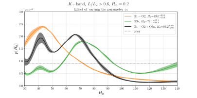
Figure 28: The same as Fig. 6 of the main text, using however $P_{\rm th}=0.2$ (left) and $P_{\rm th}=0.5$ (right). We use mask completion, multiplicative completion, and K-band luminosity weighting.

E.2 Comparison of B band and K band luminosity weighting

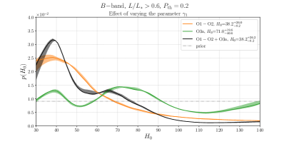
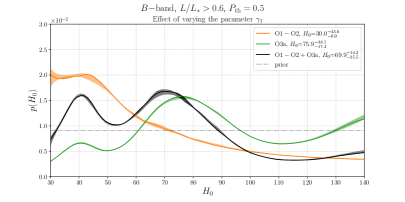
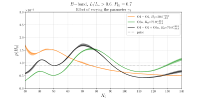
Figure 29: The posterior on $H_{0}$ in B band for $P_{\rm th}=0.2$ (upper left), $P_{\rm th}=0.5$ (upper right) and $P_{\rm th}=0.7$ (lower panel), using mask completeness and multiplicative completion.

Fig. 29 shows the analogous plot for B band, using $P_{\rm th}=0.2$ (upper left), $P_{\rm th}=0.5$ (upper right) and $P_{\rm th}=0.7$ (lower panel). We see that the situation for the dependence on $P_{\rm th}$ is similar to that in K band, with a spurious peak at $H_{0}\sim 40\,\,{\rm km}\,{\rm s}^{-1}\,{\rm Mpc}^{-1}$ that significantly decreases as we increase $P_{\rm th}$. However, in B band, for the same value of $P_{\rm th}$, the spurious peak is stronger than in K band. For $P_{\rm th}=0.2$ it is the dominant peak, and at $P_{\rm th}=0.5$ the peak at low $H_{0}$ is still basically as large as that at $H_{0}\sim 70\,\,{\rm km}\,{\rm s}^{-1}\,{\rm Mpc}^{-1}$ (while, in K band, it was just a small bump), and it is still well visible for $P_{\rm th}=0.7$, when in K band it had basically disappeared. Thus, to mitigate this bias, in B band one should set a higher value of $P_{\rm th}$, compared to K band (for instance, the plot with $P_{\rm th}=0.2$ in K band looks quite similar to that with $P_{\rm th}=0.5$ in B band, and that with $P_{\rm th}=0.5$ in K band looks quite similar to that with $P_{\rm th}=0.7$ in B band). For this reason, we use K band in our baseline model. Still, once a relatively high threshold such as $P_{\rm th}=0.7$ has been chosen, the results for the maximum a posteriori value and the corresponding highest density interval in B band become already comparable to those in K band. In particular, for $P_{\rm th}=0.7$, in B band, we get

$$H_{0}=70.8^{+20.3}_{-34.4}\,\qquad\qquad(\mbox{\rm B band})\,.$$ (E.1)

which is quite consistent with the K band result (4.1), although with a somewhat larger error.

E.3 Comparison of different completeness measures and completion procedures

We finally compare the results using our two ways of quantifying the quasi-completeness of a catalog, namely mask completeness and cone completeness, and our two ways of adding the missing galaxy, homogeneous and multiplicative completion (as explained in the text, what we call simply multiplicative completion in the result section, is actually the interpolation between multiplicative and homogeneous completion).

The results using cone completeness are shown in Fig. 30, for homogeneous completion (left) and multiplicative completion (right), where the shaded bands represent the effect of varying $\gamma_{1}$. The corresponding values for the maximum a posteriori value and the highest density interval, using the combined O1+O2+O3a data, are

$$H_{0} = 67.3^{+27.1}_{-21.4}\,\qquad\qquad(\mbox{\rm cone completeness, homogeneous completion})\,,$$ (E.2)

$$H_{0} = 67.3^{+28.4}_{-18.5}\,\qquad\qquad(\mbox{\rm cone completeness, multiplicative completion})\,,$$ (E.3)

These should be compared with our baseline result using mask completion and multiplicative completion, given by Fig. 6 and eq. (4.1). We see that the overall shapes of the posteriors in Fig. 30 are visually almost identical to those in Fig. 6 and the maximum a posteriori value of $H_{0}$ is exactly the same, within the digits given. The highest density intervals are also very similar, although slightly broader, compared to that given in eq. (4.1). The same happens using our default choice of mask completion as a measure of completeness, but filling the missing galaxies according to homogeneous completion, that gives again a very similar posterior, and

$$H_{0}=67.3^{+26.7}_{-22.3}\,\qquad\qquad(\mbox{\rm mask completeness, homogeneous completion})\,,$$ (E.4)

This shows that the different prescriptions that we have explored, both for quantifying the semi-local completeness of the catalog, and for distributing the missing galaxies, give very consistent results, at least for the relatively large completeness threshold $P_{\rm th}=0.7$ that we must anyhow chose, according to the discussion in sect. E.1.

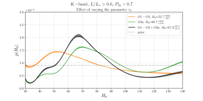
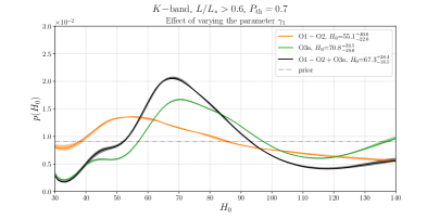
Figure 30: The posterior for $H_{0}$ using cone completeness and homogeneous completion (left) and cone completeness and multiplicative completion (right), while still keeping our default choices, K band and $P_{\rm th}=0.7$.

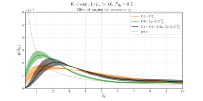
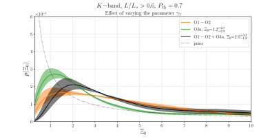
Figure 31: The posterior for $\Xi_{0}$ using cone completeness and homogeneous completion (left) and cone completeness and multiplicative completion (right), while still keeping our default choices, K band and $P_{\rm th}=0.7$.

The same situation takes place for $\Xi_{0}$. In Fig. 31 we show the posteriors for $\Xi_{0}$ using cone completeness and homogeneous completion (left) and cone completeness and multiplicative completion (right), which are visually identical to that in Fig. 12. The corresponding values for the maximum a posteriori value and the highest density interval, using the combined O1+O2+O3a data, are

$$\Xi_{0} = 2.3^{+3.2}_{-1.3}\,\qquad\qquad(\mbox{\rm cone completeness, homogeneous completion})\,,$$ (E.5)

$$\Xi_{0} = 2.0^{+3.3}_{-1.2}\,\qquad\qquad(\mbox{\rm cone completeness, multiplicative completion})\,,$$ (E.6)

again very consistent among them and with the result given in eq. (4.11). Similarly, for mask completeness and homogeneous completion, we get

$$\Xi_{0}=2.2^{+3.3}_{-1.2}\,.$$ (E.7)

References

- [1] B. P. Abbott et al., “Observation of Gravitational Waves from a Binary Black Hole Merger,” Phys. Rev. Lett. 116 (2016) 061102, arXiv:1602.03837 [gr-qc].
- [2] B. Abbott et al., “GW170817: Observation of Gravitational Waves from a Binary Neutron Star Inspiral,” Phys. Rev. Lett. 119 (2017) 161101, arXiv:1710.05832 [gr-qc].
- [3] A. Goldstein et al., “An Ordinary Short Gamma-Ray Burst with Extraordinary Implications: Fermi-GBM Detection of GRB 170817A,” Astrophys. J. 848 (2017) L14, arXiv:1710.05446 [astro-ph.HE].
- [4] V. Savchenko et al., “INTEGRAL Detection of the First Prompt Gamma-Ray Signal Coincident with the Gravitational-wave Event GW170817,” Astrophys. J. 848 (2017) L15, arXiv:1710.05449 [astro-ph.HE].
- [5] B. P. Abbott et al., “Gravitational Waves and Gamma-rays from a Binary Neutron Star Merger: GW170817 and GRB 170817A,” Astrophys. J. 848 (2017) L13, arXiv:1710.05834 [astro-ph.HE].
- [6] LIGO Scientific, Virgo Collaboration, R. Abbott et al., “GWTC-2: Compact Binary Coalescences Observed by LIGO and Virgo During the First Half of the Third Observing Run,” arXiv:2010.14527 [gr-qc].
- [7] B. F. Schutz, “Determining the Hubble Constant from Gravitational Wave Observations,” Nature 323 (1986) 310–311.
- [8] D. E. Holz and S. A. Hughes, “Using gravitational-wave standard sirens,” Astrophys. J. 629 (2005) 15–22, arXiv:astro-ph/0504616 [astro-ph].
- [9] N. Dalal, D. E. Holz, S. A. Hughes, and B. Jain, “Short GRB and binary black hole standard sirens as a probe of dark energy,” Phys. Rev. D74 (2006) 063006, arXiv:astro-ph/0601275 [astro-ph].
- [10] C. L. MacLeod and C. J. Hogan, “Precision of Hubble constant derived using black hole binary absolute distances and statistical redshift information,” Phys. Rev. D77 (2008) 043512, arXiv:0712.0618 [astro-ph].
- [11] S. Nissanke, D. E. Holz, S. Hughes, N. Dalal, and J. L. Sievers, “Exploring short gamma-ray bursts as gravitational-wave standard sirens,” Astrophys. J. 725 (2010) 496–514, arXiv:0904.1017 [astro-ph.CO].
- [12] C. Cutler and D. E. Holz, “Ultra-high precision cosmology from gravitational waves,” Phys. Rev. D80 (2009) 104009, arXiv:0906.3752 [astro-ph.CO].
- [13] W. Del Pozzo, “Inference of the cosmological parameters from gravitational waves: application to second generation interferometers,” Phys. Rev. D86 (2012) 043011, arXiv:1108.1317 [astro-ph.CO].
- [14] S. R. Taylor and J. R. Gair, “Cosmology with the lights off: standard sirens in the Einstein Telescope era,” Phys. Rev. D86 (2012) 023502, arXiv:1204.6739 [astro-ph.CO].
- [15] H.-Y. Chen, M. Fishbach, and D. E. Holz, “A two per cent Hubble constant measurement from standard sirens within five years,” Nature 562 (2018) 545, arXiv:1712.06531 [astro-ph.CO].
- [16] S. M. Feeney, H. V. Peiris, A. R. Williamson, S. M. Nissanke, D. J. Mortlock, J. Alsing, and D. Scolnic, “Prospects for resolving the Hubble constant tension with standard sirens,” arXiv:1802.03404 [astro-ph.CO].
- [17] R. Gray et al., “Cosmological Inference using Gravitational Wave Standard Sirens: A Mock Data Challenge,” Phys. Rev. D 101 (2020) 122001, arXiv:1908.06050 [gr-qc].
- [18] B. P. Abbott et al., “A gravitational-wave standard siren measurement of the Hubble constant,” Nature 551 no. 7678, (2017) 85–88, arXiv:1710.05835 [astro-ph.CO].
- [19] A. G. Riess, S. Casertano, W. Yuan, L. M. Macri, and D. Scolnic, “Large Magellanic Cloud Cepheid Standards Provide a 1% Foundation for the Determination of the Hubble Constant and Stronger Evidence for Physics Beyond LambdaCDM,” Astrophys. J. 876 (2019) 85, arXiv:1903.07603 [astro-ph.CO].
- [20] K. C. Wong et al., “H0LiCOW – XIII. A 2.4 per cent measurement of H0 from lensed quasars: 5.3 tension between early- and late-Universe probes,” Mon. Not. Roy. Astron. Soc. 498 no. 1, (2020) 1420–1439, arXiv:1907.04869 [astro-ph.CO].
- [21] Planck Collaboration, N. Aghanim et al., “Planck 2018 results. VI. Cosmological parameters,” Astron. Astrophys. 641 (2020) A6, arXiv:1807.06209 [astro-ph.CO].
- [22] DES Collaboration, T. M. C. Abbott et al., “Dark Energy Survey Year 1 Results: Constraints on Extended Cosmological Models from Galaxy Clustering and Weak Lensing,” Phys. Rev. D99 (2019) 123505, arXiv:1810.02499 [astro-ph.CO].
- [23] R. Nair, S. Bose, and T. D. Saini, “Measuring the Hubble constant: Gravitational wave observations meet galaxy clustering,” Phys. Rev. D 98 (2018) 023502, arXiv:1804.06085 [astro-ph.CO].
- [24] S. Mukherjee, B. D. Wandelt, and J. Silk, “Probing the theory of gravity with gravitational lensing of gravitational waves and galaxy surveys,” Mon. Not. Roy. Astron. Soc. 494 no. 2, (2020) 1956–1970, arXiv:1908.08951 [astro-ph.CO].
- [25] J. Yu, Y. Wang, W. Zhao, and Y. Lu, “Hunting for the host galaxy groups of binary black holes and the application in constraining Hubble constant,” Mon. Not. Roy. Astron. Soc. 498 no. 2, (2020) 1786–1800, arXiv:2003.06586 [astro-ph.CO].
- [26] A. Vijaykumar, M. Saketh, S. Kumar, P. Ajith, and T. R. Choudhury, “Probing the large scale structure using gravitational-wave observations of binary black holes,” arXiv:2005.01111 [astro-ph.CO].
- [27] S. Mukherjee, B. D. Wandelt, S. M. Nissanke, and A. Silvestri, “Accurate and precision Cosmology with redshift unknown gravitational wave sources,” arXiv:2007.02943 [astro-ph.CO].
- [28] S. Bera, D. Rana, S. More, and S. Bose, “Incompleteness Matters Not: Inference of from Binary Black Hole–Galaxy Cross-correlations,” Astrophys. J. 902 (2020) 79, arXiv:2007.04271 [astro-ph.CO].
- [29] S. Mukherjee, B. D. Wandelt, and J. Silk, “Testing the general theory of relativity using gravitational wave propagation from dark standard sirens,” arXiv:2012.15316 [astro-ph.CO].
- [30] S. Borhanian, A. Dhani, A. Gupta, K. Arun, and B. Sathyaprakash, “Dark Sirens to Resolve the Hubble-Lemaître Tension,” Astrophys. J. Lett. 905 (2020) L28, arXiv:2007.02883 [astro-ph.CO].
- [31] M. Fishbach et al., “A Standard Siren Measurement of the Hubble Constant from GW170817 without the Electromagnetic Counterpart,” Astrophys. J. Lett. 871 (2019) L13, arXiv:1807.05667 [astro-ph.CO].
- [32] DES, LIGO Scientific, Virgo Collaboration, M. Soares-Santos et al., “First Measurement of the Hubble Constant from a Dark Standard Siren using the Dark Energy Survey Galaxies and the LIGO/Virgo Binary–Black-hole Merger GW170814,” Astrophys. J. Lett. 876 (2019) L7, arXiv:1901.01540 [astro-ph.CO].
- [33] A. Palmese et al., “A statistical standard siren measurement of the Hubble constant from the LIGO/Virgo gravitational wave compact object merger GW190814 and Dark Energy Survey galaxies,” arXiv:2006.14961 [astro-ph.CO].
- [34] LIGO Scientific, Virgo Collaboration, B. Abbott et al., “A gravitational-wave measurement of the Hubble constant following the second observing run of Advanced LIGO and Virgo,” arXiv:1908.06060 [astro-ph.CO].
- [35] E. Belgacem, Y. Dirian, S. Foffa, and M. Maggiore, “The gravitational-wave luminosity distance in modified gravity theories,” Phys. Rev. D97 (2018) 104066, arXiv:1712.08108 [astro-ph.CO].
- [36] E. Belgacem, Y. Dirian, S. Foffa, and M. Maggiore, “Modified gravitational-wave propagation and standard sirens,” Phys. Rev. D98 (2018) 023510, arXiv:1805.08731 [gr-qc].
- [37] C. de Rham and S. Melville, “Gravitational Rainbows: LIGO and Dark Energy at its Cutoff,” Phys. Rev. Lett. 121 (2018) 221101, arXiv:1806.09417 [hep-th].
- [38] P. Creminelli and F. Vernizzi, “Dark Energy after GW170817 and GRB170817A,” Phys. Rev. Lett. 119 (2017) 251302, arXiv:1710.05877 [astro-ph.CO].
- [39] J. Sakstein and B. Jain, “Implications of the Neutron Star Merger GW170817 for Cosmological Scalar-Tensor Theories,” Phys. Rev. Lett. 119 (2017) 251303, arXiv:1710.05893 [astro-ph.CO].
- [40] J. M. Ezquiaga and M. Zumalacárregui, “Dark Energy After GW170817: Dead Ends and the Road Ahead,” Phys. Rev. Lett. 119 (2017) 251304, arXiv:1710.05901 [astro-ph.CO].
- [41] S. Boran, S. Desai, E. O. Kahya, and R. P. Woodard, “GW170817 Falsifies Dark Matter Emulators,” Phys. Rev. D 97 (2018) 041501, arXiv:1710.06168 [astro-ph.HE].
- [42] T. Baker, E. Bellini, P. G. Ferreira, M. Lagos, J. Noller, and I. Sawicki, “Strong constraints on cosmological gravity from GW170817 and GRB 170817A,” Phys. Rev. Lett. 119 (2017) 251301, arXiv:1710.06394 [astro-ph.CO].
- [43] I. D. Saltas, I. Sawicki, L. Amendola, and M. Kunz, “Anisotropic Stress as a Signature of Nonstandard Propagation of Gravitational Waves,” Phys. Rev. Lett. 113 (2014) 191101, arXiv:1406.7139 [astro-ph.CO].
- [44] L. Lombriser and A. Taylor, “Breaking a Dark Degeneracy with Gravitational Waves,” JCAP 1603 (2016) 031, arXiv:1509.08458 [astro-ph.CO].
- [45] A. Nishizawa, “Generalized framework for testing gravity with gravitational-wave propagation. I. Formulation,” Phys. Rev. D97 (2018) 104037, arXiv:1710.04825 [gr-qc].
- [46] S. Arai and A. Nishizawa, “Generalized framework for testing gravity with gravitational-wave propagation. II. Constraints on Horndeski theory,” Phys. Rev. D97 (2018) 104038, arXiv:1711.03776 [gr-qc].
- [47] L. Amendola, I. Sawicki, M. Kunz, and I. D. Saltas, “Direct detection of gravitational waves can measure the time variation of the Planck mass,” JCAP 1808 (2018) 030, arXiv:1712.08623 [astro-ph.CO].
- [48] LISA Cosmology Working Group Collaboration, E. Belgacem et al., “Testing modified gravity at cosmological distances with LISA standard sirens,” JCAP 1907 (2019) 024, arXiv:1906.01593 [astro-ph.CO].
- [49] M. Maggiore, Gravitational Waves. Vol. 1: Theory and Experiments. Oxford Master Series in Physics. Oxford University Press, 2007. http://www.oup.com/uk/catalogue/?ci=9780198570745.
- [50] M. Chevallier and D. Polarski, “Accelerating universes with scaling dark matter,” Int.J.Mod.Phys. D10 (2001) 213–224, arXiv:gr-qc/0009008 [gr-qc].
- [51] E. V. Linder, “Exploring the expansion history of the universe,” Phys.Rev.Lett. 90 (2003) 091301, arXiv:astro-ph/0208512 [astro-ph].
- [52] E. Belgacem, Y. Dirian, S. Foffa, E. J. Howell, M. Maggiore, and T. Regimbau, “Cosmology and dark energy from joint gravitational wave-GRB observations,” JCAP 1908 (2019) 015, arXiv:1907.01487 [astro-ph.CO].
- [53] W. M. Farr, M. Fishbach, J. Ye, and D. Holz, “A Future Percent-Level Measurement of the Hubble Expansion at Redshift 0.8 With Advanced LIGO,” Astrophys. J. Lett. 883 no. 2, (2019) L42, arXiv:1908.09084 [astro-ph.CO].
- [54] M. Punturo et al., “The Einstein Telescope: A third-generation gravitational wave observatory,” Class. Quant. Grav. 27 (2010) 194002.
- [55] M. Maggiore et al., “Science Case for the Einstein Telescope,” JCAP 03 (2020) 050, arXiv:1912.02622 [astro-ph.CO].
- [56] D. Reitze et al., “Cosmic Explorer: The U.S. Contribution to Gravitational-Wave Astronomy beyond LIGO,” Bull. Am. Astron. Soc. 51 (2019) 035, arXiv:1907.04833 [astro-ph.IM].
- [57] B. S. Sathyaprakash, B. F. Schutz, and C. Van Den Broeck, “Cosmography with the Einstein Telescope,” Class. Quant. Grav. 27 (2010) 215006, arXiv:0906.4151 [astro-ph.CO].
- [58] W. Zhao, C. Van Den Broeck, D. Baskaran, and T. G. F. Li, “Determination of Dark Energy by the Einstein Telescope: Comparing with CMB, BAO and SNIa Observations,” Phys. Rev. D83 (2011) 023005, arXiv:1009.0206 [astro-ph.CO].
- [59] P. Amaro-Seoane et al., “Laser Interferometer Space Antenna,” arXiv:1702.00786 [astro-ph.IM].
- [60] E. Belgacem, Y. Dirian, A. Finke, S. Foffa, and M. Maggiore, “Nonlocal gravity and gravitational-wave observations,” JCAP 1911 (2019) 022, arXiv:1907.02047 [astro-ph.CO].
- [61] E. Belgacem, Y. Dirian, A. Finke, S. Foffa, and M. Maggiore, “Gravity in the infrared and effective nonlocal models,” JCAP 04 (2020) 010, arXiv:2001.07619 [astro-ph.CO].
- [62] M. Cantiello et al., “A Precise Distance to the Host Galaxy of the Binary Neutron Star Merger GW170817 Using Surface Brightness Fluctuations,” Astrophys. J. Lett. 854 no. 2, (2018) L31, arXiv:1801.06080 [astro-ph.GA].
- [63] M. Lagos, M. Fishbach, P. Landry, and D. E. Holz, “Standard sirens with a running Planck mass,” Phys. Rev. D99 (2019) 083504, arXiv:1901.03321 [astro-ph.CO].
- [64] E. Bellini and I. Sawicki, “Maximal freedom at minimum cost: linear large-scale structure in general modifications of gravity,” JCAP 07 (2014) 050, arXiv:1404.3713 [astro-ph.CO].
- [65] K. Pardo, M. Fishbach, D. E. Holz, and D. N. Spergel, “Limits on the number of spacetime dimensions from GW170817,” JCAP 1807 (2018) 048, arXiv:1801.08160 [gr-qc].
- [66] D. Bertacca, A. Raccanelli, N. Bartolo, and S. Matarrese, “Cosmological perturbation effects on gravitational-wave luminosity distance estimates,” Phys. Dark Univ. 20 (2018) 32–40, arXiv:1702.01750 [gr-qc].
- [67] M. Kalomenopoulos, S. Khochfar, J. Gair, and S. Arai, “Mapping the inhomogeneous Universe with Standard Sirens: Degeneracy between inhomogeneity and modified gravity theories,” arXiv:2007.15020 [astro-ph.CO].
- [68] LIGO Scientific, Virgo Collaboration, R. Abbott et al., “GW190814: Gravitational Waves from the Coalescence of a 23 Solar Mass Black Hole with a 2.6 Solar Mass Compact Object,” Astrophys. J. 896 (2020) L44, arXiv:2006.12611 [astro-ph.HE].
- [69] DES Collaboration, R. Morgan et al., “Constraints on the Physical Properties of GW190814 through Simulations Based on DECam Follow-up Observations by the Dark Energy Survey,” Astrophys. J. 901 no. 1, (2020) 83, arXiv:2006.07385 [astro-ph.HE].
- [70] M. Graham et al., “Candidate Electromagnetic Counterpart to the Binary Black Hole Merger Gravitational Wave Event S190521g,” Phys. Rev. Lett. 124 no. 25, (2020) 251102, arXiv:2006.14122 [astro-ph.HE].
- [71] G. Ashton, K. Ackley, I. M. Hernandez, and B. Piotrzkowski, “Current observations are insufficient to confidently associate the binary black hole merger GW190521 with AGN J124942.3+344929,” arXiv:2009.12346 [astro-ph.HE].
- [72] S. Mastrogiovanni, L. Haegel, C. Karathanasis, I. Magana-Hernandez, and D. Steer, “Gravitational wave friction in light of GW170817 and GW190521,” arXiv:2010.04047 [gr-qc].
- [73] M. Maggiore, “Phantom dark energy from nonlocal infrared modifications of general relativity,” Phys.Rev. D89 (2014) 043008, arXiv:1307.3898 [hep-th].
- [74] M. Maggiore, “Nonlocal Infrared Modifications of Gravity. A Review,” Fundam. Theor. Phys. 187 (2017) 221–281, arXiv:1606.08784 [hep-th].
- [75] S. Foffa, M. Maggiore, and E. Mitsou, “Cosmological dynamics and dark energy from non-local infrared modifications of gravity,” Int.J.Mod.Phys. A29 (2014) 1450116, arXiv:1311.3435 [hep-th].
- [76] A. Kehagias and M. Maggiore, “Spherically symmetric static solutions in a non-local infrared modification of General Relativity,” JHEP 1408 (2014) 029, arXiv:1401.8289 [hep-th].
- [77] M. Maggiore and M. Mancarella, “Non-local gravity and dark energy,” Phys.Rev. D90 (2014) 023005, arXiv:1402.0448 [hep-th].
- [78] S. Nesseris and S. Tsujikawa, “Cosmological perturbations and observational constraints on nonlocal massive gravity,” Phys.Rev. D90 (2014) 024070, arXiv:1402.4613 [astro-ph.CO].
- [79] Y. Dirian, S. Foffa, N. Khosravi, M. Kunz, and M. Maggiore, “Cosmological perturbations and structure formation in nonlocal infrared modifications of general relativity,” JCAP 1406 (2014) 033, arXiv:1403.6068 [astro-ph.CO].
- [80] A. Barreira, B. Li, W. A. Hellwing, C. M. Baugh, and S. Pascoli, “Nonlinear structure formation in Nonlocal Gravity,” JCAP 1409 (2014) 031, arXiv:1408.1084 [astro-ph.CO].
- [81] Y. Dirian, S. Foffa, M. Kunz, M. Maggiore, and V. Pettorino, “Non-local gravity and comparison with observational datasets,” JCAP 1504 (2015) 044, arXiv:1411.7692 [astro-ph.CO].
- [82] Y. Dirian, S. Foffa, M. Kunz, M. Maggiore, and V. Pettorino, “Non-local gravity and comparison with observational datasets. II. Updated results and Bayesian model comparison with CDM,” JCAP 1605 (2016) 068, arXiv:1602.03558 [astro-ph.CO].
- [83] Y. Dirian, “Changing the Bayesian prior: Absolute neutrino mass constraints in nonlocal gravity,” Phys. Rev. D96 (2017) 083513, arXiv:1704.04075 [astro-ph.CO].
- [84] E. Belgacem, Y. Dirian, S. Foffa, and M. Maggiore, “Nonlocal gravity. Conceptual aspects and cosmological predictions,” JCAP 1803 (2018) 002, arXiv:1712.07066 [hep-th].
- [85] E. Belgacem, A. Finke, A. Frassino, and M. Maggiore, “Testing nonlocal gravity with Lunar Laser Ranging,” JCAP 1902 (2019) 035, arXiv:1812.11181 [gr-qc].
- [86] M. Ishak et al., “Modified Gravity and Dark Energy models Beyond CDM Testable by LSST,” arXiv:1905.09687 [astro-ph.CO].
- [87] I. Mandel, W. M. Farr, and J. R. Gair, “Extracting distribution parameters from multiple uncertain observations with selection biases,” Mon. Not. Roy. Astron. Soc. 486 (2019) 1086–1093, arXiv:1809.02063 [physics.data-an].
- [88] S. Vasylyev and A. Filippenko, “A Measurement of the Hubble Constant using Gravitational Waves from the Neutron-Star Black-Hole Candidate GW190814,” arXiv:2007.11148 [astro-ph.CO].
- [89] T. J. Loredo, “Accounting for source uncertainties in analyses of astronomical survey data,” AIP Conf. Proc. 735 (2004) 195, arXiv:astro-ph/0409387.
- [90] M. R. Adams, N. J. Cornish, and T. B. Littenberg, “Astrophysical Model Selection in Gravitational Wave Astronomy,” Phys. Rev. D 86 (2012) 124032, arXiv:1209.6286 [gr-qc].
- [91] E. Thrane and C. Talbot, “An introduction to Bayesian inference in gravitational-wave astronomy: parameter estimation, model selection, and hierarchical models,” Publ. Astron. Soc. Austral. 36 (2019) e010, arXiv:1809.02293 [astro-ph.IM].
- [92] S. Vitale, D. Gerosa, W. M. Farr, and S. R. Taylor, “Inferring the properties of a population of compact binaries in presence of selection effects,” arXiv:2007.05579 [astro-ph.IM].
- [93] S. R. Taylor, J. R. Gair, and I. Mandel, “Hubble without the Hubble: Cosmology using advanced gravitational-wave detectors alone,” Phys. Rev. D85 (2012) 023535, arXiv:1108.5161 [gr-qc].
- [94] S. Mastrogiovanni, K. Leyde, C. Karathanasis, E. Chassande-Mottin, D. A. Steer, J. Gair, A. Ghosh, R. Gray, S. Mukherjee, and S. Rinaldi, “Cosmology in the dark: On the importance of source population models for gravitational-wave cosmology,” arXiv:2103.14663 [gr-qc].
- [95] L. P. Singer et al., “Going the Distance: Mapping Host Galaxies of LIGO and Virgo Sources in Three Dimensions Using Local Cosmography and Targeted Follow-up,” Astrophys. J. Lett. 829 (2016) L15, arXiv:1603.07333 [astro-ph.HE].
- [96] L. P. Singer et al., “Supplement: Going the Distance: Mapping Host Galaxies of LIGO and Virgo Sources in Three Dimensions Using Local Cosmography and Targeted Follow-up,” Astrophys. J. Suppl. 226 (2016) 10, arXiv:1605.04242 [astro-ph.IM].
- [97] K. Gorski, E. Hivon, A. Banday, B. Wandelt, F. Hansen, M. Reinecke, and M. Bartelman, “HEALPix - A Framework for high resolution discretization, and fast analysis of data distributed on the sphere,” Astrophys. J. 622 (2005) 759, arXiv:astro-ph/0409513.
- [98] M. Fishbach, Z. Doctor, T. Callister, B. Edelman, J. Ye, R. Essick, W. M. Farr, B. Farr, and D. E. Holz, “When are LIGO/Virgo’s Big Black-Hole Mergers?,” arXiv:2101.07699 [astro-ph.HE].
- [99] G. Dálya, G. Galgóczi, L. Dobos, Z. Frei, I. S. Heng, R. Macas, C. Messenger, P. Raffai, and R. S. de Souza, “GLADE: A galaxy catalogue for multimessenger searches in the advanced gravitational-wave detector era,” Mon. Not. Roy. Astron. Soc. 479 (2018) 2374–2381, arXiv:1804.05709 [astro-ph.HE].
- [100] C. J. Conselice, A. Wilkinson, K. Duncan, and A. Mortlock, “The Evolution of Galaxy Number Density at and its Implications,” Astrophys. J. 830 (2016) 83, arXiv:1607.03909 [astro-ph.GA].
- [101] M. Fishbach, D. E. Holz, and W. M. Farr, “Does the Black Hole Merger Rate Evolve with Redshift?,” Astrophys. J. Lett. 863 (2018) L41, arXiv:1805.10270 [astro-ph.HE].
- [102] T. Callister, M. Fishbach, D. Holz, and W. Farr, “Shouts and Murmurs: Combining Individual Gravitational-Wave Sources with the Stochastic Background to Measure the History of Binary Black Hole Mergers,” Astrophys. J. Lett. 896 no. 2, (2020) L32, arXiv:2003.12152 [astro-ph.HE].
- [103] P. Madau and M. Dickinson, “Cosmic Star Formation History,” Ann. Rev. Astron. Astrophys. 52 (2014) 415–486, arXiv:1403.0007 [astro-ph.CO].
- [104] P. Madau and T. Fragos, “Radiation Backgrounds at Cosmic Dawn: X-Rays from Compact Binaries,” Astrophys. J. 840 (2017) 39, arXiv:1606.07887 [astro-ph.GA].
- [105] LIGO Scientific, Virgo Collaboration, R. Abbott et al., “Population Properties of Compact Objects from the Second LIGO-Virgo Gravitational-Wave Transient Catalog,” arXiv:2010.14533 [astro-ph.HE].
- [106] LIGO Scientific, Virgo Collaboration, B. Abbott et al., “GWTC-1: A Gravitational-Wave Transient Catalog of Compact Binary Mergers Observed by LIGO and Virgo during the First and Second Observing Runs,” Phys. Rev. X 9 (2019) 031040, arXiv:1811.12907 [astro-ph.HE].
- [107] G. Pratten, S. Husa, C. Garcia-Quiros, M. Colleoni, A. Ramos-Buades, H. Estelles, and R. Jaume, “Setting the cornerstone for a family of models for gravitational waves from compact binaries: The dominant harmonic for nonprecessing quasicircular black holes,” Phys. Rev. D 102 (2020) 064001, arXiv:2001.11412 [gr-qc].
- [108] H.-Y. Chen and D. E. Holz, “The Loudest Gravitational Wave Events,” arXiv:1409.0522 [gr-qc].
- [109] E. Calabrese, N. Battaglia, and D. N. Spergel, “Testing Gravity with Gravitational Wave Source Counts,” Class. Quant. Grav. 33 (2016) 165004, arXiv:1602.03883 [gr-qc].
- [110] J. García-Bellido, S. Nesseris, and M. Trashorras, “Gravitational wave source counts at high redshift and in models with extra dimensions,” JCAP 07 (2016) 021, arXiv:1603.05616 [astro-ph.CO].
- [111] J. María Ezquiaga, “Hearing gravity from the cosmos: GWTC-2 probes general relativity at cosmological scales,” arXiv:2104.05139 [astro-ph.CO].
- [112] T. W. Keelin, “The metalog distributions,” Decision Analysis 13 no. 4, (2016) 243–277, https://doi.org/10.1287/deca.2016.0338.
- [113] A. C. Crook, J. P. Huchra, N. Martimbeau, K. L. Masters, T. Jarrett, and L. M. Macri, “Groups of Galaxies in the Two Micron All-Sky Redshift Survey,” Astrophys. J. 655 (2007) 790, arXiv:astro-ph/0610732.
- [114] S. Mukherjee, G. Lava ux, F. R. Bouchet, J. Jasche, B. D. Wandelt, S. M. Nissanke, F. Leclercq, and K. Hotokezaka, “Velocity correction for Hubble constant measurements from standard sirens,” arXiv:1909.08627 [astro-ph.CO].
- [115] H.-Y. Chen, C.-J. Haster, S. Vitale, W. M. Farr, and M. Isi, “A Standard Siren Cosmological Measurement from the Potential GW190521 Electromagnetic Counterpart ZTF19abanrhr,” arXiv:2009.14057 [astro-ph.CO].
- [116] K. Mooley, A. Deller, O. Gottlieb, E. Nakar, G. Hallinan, S. Bourke, D. Frail, A. Horesh, A. Corsi, and K. Hotokezaka, “Superluminal motion of a relativistic jet in the neutron-star merger GW170817,” Nature 561 no. 7723, (2018) 355–359, arXiv:1806.09693 [astro-ph.HE].
- [117] S. Mastrogiovanni, R. Duque, E. Chassande-Mottin, F. Daigne, and R. Mochkovitch, “What role will binary neutron star merger afterglows play in multimessenger cosmology?,” arXiv:2012.12836 [astro-ph.HE].
- [118] N. Khetan et al., “A new measurement of the Hubble constant using Type Ia supernovae calibrated with surface brightness fluctuations,” arXiv:2008.07754 [astro-ph.CO].
- [119] LIGO Scientific, Virgo Collaboration, R. Abbott et al., “GW190521: A Binary Black Hole Merger with a Total Mass of ,” Phys. Rev. Lett. 125 no. 10, (2020) 101102, arXiv:2009.01075 [gr-qc].
- [120] LIGO Scientific, Virgo Collaboration, R. Abbott et al., “Properties and Astrophysical Implications of the 150 M⊙ Binary Black Hole Merger GW190521,” Astrophys. J. Lett. 900 no. 1, (2020) L13, arXiv:2009.01190 [astro-ph.HE].
- [121] B. McKernan, K. E. S. Ford, I. Bartos, M. J. Graham, W. Lyra, S. Marka, Z. Marka, N. P. Ross, D. Stern, and Y. Yang, “Ram-pressure stripping of a kicked Hill sphere: Prompt electromagnetic emission from the merger of stellar mass black holes in an AGN accretion disk,” Astrophys. J. Lett. 884 no. 2, (2019) L50, arXiv:1907.03746 [astro-ph.HE].
- [122] M. Fishbach and D. E. Holz, “Minding the gap: GW190521 as a straddling binary,” Astrophys. J. Lett. 904 no. 2, (2020) L26, arXiv:2009.05472 [astro-ph.HE].
- [123] V. Gayathri, J. Healy, J. Lange, B. O’Brien, M. Szczepanczyk, I. Bartos, M. Campanelli, S. Klimenko, C. Lousto, and R. O’Shaughnessy, “GW190521 as a Highly Eccentric Black Hole Merger,” arXiv:2009.05461 [astro-ph.HE].
- [124] WMAP Collaboration, G. Hinshaw et al., “Five-Year Wilkinson Microwave Anisotropy Probe (WMAP) Observations: Data Processing, Sky Maps, and Basic Results,” Astrophys. J. Suppl. 180 (2009) 225–245, arXiv:0803.0732 [astro-ph].
- [125] D. C. Pan, M. S. Vogeley, F. Hoyle, Y.-Y. Choi, and C. Park, “Cosmic Voids in Sloan Digital Sky Survey Data Release 7,” Mon. Not. Roy. Astron. Soc. 421 (2012) 926–934, arXiv:1103.4156 [astro-ph.CO].
- [126] N. I. Libeskind et al., “Tracing the cosmic web,” Mon. Not. Roy. Astron. Soc. 473 (2018) 1195–1217, arXiv:1705.03021 [astro-ph.CO].
- [127] N. Gehrels, J. K. Cannizzo, J. Kanner, M. M. Kasliwal, S. Nissanke, and L. P. Singer, “Galaxy Strategy for LIGO-Virgo Gravitational Wave Counterpart Searches,” Astrophys. J. 820 no. 2, (2016) 136, arXiv:1508.03608 [astro-ph.HE].
- [128] I. Arcavi et al., “Optical Follow-up of Gravitational-wave Events with Las Cumbres Observatory,” Astrophys. J. Lett. 848 (2017) L33, arXiv:1710.05842 [astro-ph.HE].
- [129] C. Kochanek, M. Pahre, E. Falco, J. Huchra, J. Mader, T. Jarrett, T. Chester, R. Cutri, and S. Schneider, “The k-band galaxy luminosity function,” Astrophys. J. 560 (2001) 566–579, arXiv:astro-ph/0011456.
- [130] J. Huchra, N. Martimbeau, T. Jarrett, R. Cutri, M. Skrutskie, S. Schneider, R. Steining, L. Macri, J. Mader, and T. George, “2MASS and the Nearby Universe,” in Maps of the Cosmos, M. Colless, L. Staveley-Smith, and R. A. Stathakis, eds., vol. 216 of IAU Symposium, pp. 170–179. Jan., 2005.
- [131] T. Lambert, R. Kraan-Korteweg, T. Jarrett, and L. Macri, “The 2MASS redshift survey galaxy group catalogue derived from a graph-theory based friends-of-friends algorithm,” Mon. Not. Roy. Astron. Soc. 497 no. 3, (2020) 2954–2973, arXiv:2007.00581 [astro-ph.GA].
- [132] Y. Lu, X. Yang, F. Shi, H. Mo, D. Tweed, H. Wang, Y. Zhang, S. Li, and S. Lim, “Galaxy groups in the 2MASS Redshift Survey,” Astrophys. J. 832 (2016) 39, arXiv:1607.03982 [astro-ph.GA].
- [133] LIGO Scientific, VIRGO Collaboration, J. Abadie et al., “Predictions for the Rates of Compact Binary Coalescences Observable by Ground-based Gravitational-wave Detectors,” Class. Quant. Grav. 27 (2010) 173001, arXiv:1003.2480 [astro-ph.HE].
- [134] D. Wysocki, J. Lange, and R. O’Shaughnessy, “Reconstructing phenomenological distributions of compact binaries via gravitational wave observations,” Phys. Rev. D 100 (2019) 043012, arXiv:1805.06442 [gr-qc].
- [135] L. S. Finn and D. F. Chernoff, “Observing binary inspiral in gravitational radiation: One interferometer,” Phys. Rev. D 47 (1993) 2198–2219, arXiv:gr-qc/9301003.