Exploring Cross-Image Pixel Contrast for Semantic Segmentation

Abstract

Current semantic segmentation methods focus only on mining “local” context, , dependencies between pixels within individual images, by context-aggregation modules (, dilated convolution, neural attention) or structure-aware${}_{\!}$ optimization${}_{\!}$ criteria${}_{\!}$ (, IoU-like${}_{\!}$ loss).${}_{\!}$ However, they ignore “global” context of the training data, , rich semantic relations between pixels across different images. Inspired by recent advance in unsupervised contrastive representation learning, we propose a pixel-wise contrastive algorithm for semantic segmentation in the fully supervised setting. The core idea is to enforce pixel embeddings belonging to a same semantic class to be more similar than embeddings from different classes. It raises a pixel-wise metric learning paradigm for semantic segmentation, by explicitly exploring the structures of labeled pixels, which were rarely explored before. Our method can be effortlessly incorporated into existing segmentation frameworks without extra overhead during testing. We experimentally show that, with famous segmentation models${}_{\!}$ (,${}_{\!}$ DeepLabV3,${}_{\!}$ HRNet,${}_{\!}$ OCR) and backbones${}_{\!}$ (, ResNet, HRNet), our method brings performance improvements across diverse datasets (, Cityscapes, PASCAL-Context, COCO-Stuff, CamVid). We expect this work will encourage our community to rethink the current de facto training paradigm in semantic segmentation.

1 Introduction

Semantic segmentation, which aims to infer semantic labels for all pixels in an image, is a fundamental problem in computer vision. In the last decade, semantic segmentation has achieved remarkable progress, driven by the availability of large-scale datasets (, Cityscapes [15]) and rapid evolution of convolutional networks (, VGG [62], ResNet [30]) as well as segmentation models (, fully convolutional network (FCN) [50]). In particular, FCN [50] is the cornerstone of modern deep learning techniques for segmentation, due to its unique advantage in end-to-end pixel-wise representation learning. However, its spatial invariance nature hinders the ability of modeling useful context among pixels (within images). Thus a main stream of subsequent effort delves into network designs for effective context aggregation, , dilated convolution​ [78, 8, 9], spatial pyramid pooling​ [82], multi-layer feature fusion​ [57, 45] and neural attention​ [33, 22]. In addition, as the widely adopted pixel-wise cross entropy loss fundamentally lacks the spatial discrimination power, some alternative optimization criteria are proposed to explicitly address object structures during segmentation network training [38, 2, 84].

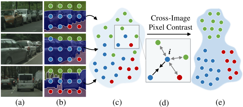
Figure 1: ​Main${}_{\!}$ idea.${}_{\!}$ Current${}_{\!}$ segmentation${}_{\!}$ models${}_{\!}$ learn to map pixels (b) to an embedding space (c), yet ignoring intrinsic structures of labeled data (, inter-image relations among pixels from a same class, noted with same color in ​(b)). Pixel-wise contrastive learning is introduced to foster a new training paradigm (d), by explicitly addressing intra-class compactness and inter-class dispersion. Each pixel (embedding) $i$ is pulled closer () to pixels () of the same class, but pushed far () from pixels ( ) from other${}_{\!}$ classes.${}_{\!}$ Thus${}_{\!}$ a${}_{\!}$ better-structured embedding${}_{\!}$ space (e) is derived, eventually${}_{\!}$ boosting the${}_{\!}$ performance${}_{\!}$ of${}_{\!}$ segmentation${}_{\!}$ models.${}_{\!\!}$

Basically, these segmentation models (excepting [35]) utilize deep architectures to project image pixels into a highly non-linear embedding space (Fig.​ 1(c)). However, they typically learn the embedding space that only makes use of “local” context around pixel samples (, pixel dependencies within individual images), but ignores “global” context of the whole dataset (, pixel semantic relations across images). Hence, an essential issue has been long ignored in the field: what should a good segmentation embedding space look like? Ideally, it should not only 1) address the categorization ability of individual pixel embeddings, but also${}_{\!}$ 2)${}_{\!}$ be${}_{\!}$ well${}_{\!}$ structured${}_{\!}$ to${}_{\!}$ address intra-class compactness and inter-class dispersion. With regard to 2), pixels from a same class should be closer than those from different classes, in the embedding space. Prior studies​ [48, 59] in representation learning also suggested that encoding intrinsic structures of training data (, 2)) would facilitate feature discriminativeness (, 1)). So we speculate that, although existing algorithms have achieved impressive performance, it is possible to learn a better structured pixel embedding space by considering both 1) and 2).

Recent advance in unsupervised representation learning [12, 29] can be ascribed to the resurgence of contrastive learning – an essential branch of deep metric learning [37]. The core idea is “learn to compare”: given an anchor point, distinguish a similar (or positive) sample from a set of dissimilar (or negative) samples, in a projected embedding space. Especially, in the field of computer vision, the contrast is evaluated based on image feature vectors; the augmented version of an anchor image is viewed as a positive, while all the other images in the dataset act as negatives.

The great success of unsupervised contrastive learning and our aforementioned speculation together motivate us to rethink the current de facto training paradigm in semantic segmentation. Basically, the power of unsupervised contrastive learning roots from the structured comparison loss, which takes the advantage of the context within the training data. With this insight, we propose a pixel-wise contrastive algorithm for more effective dense representation learning in the fully supervised setting. Specifically, in addition to adopting the pixel-wise cross entropy loss to address class discrimination (, property 1)), we utilize a pixel-wise contrastive loss to further shape the pixel embedding space, through exploring the structural information of labeled pixel samples (, property 2)). The idea of the pixel-wise contrastive loss is to compute pixel-to-pixel contrast: enforce embeddings to be similar for positive pixels, and dissimilar for negative ones. As the pixel-level categorical information is given during training, the positive samples are the pixels belonging to a same class, and the negatives are the pixels from different classes (Fig.​ 1(d)). In this way, the global property of the embedding space can be captured (Fig.​ 1(e)) for better reflecting intrinsic structures of training data and enabling more accurate segmentation predictions.

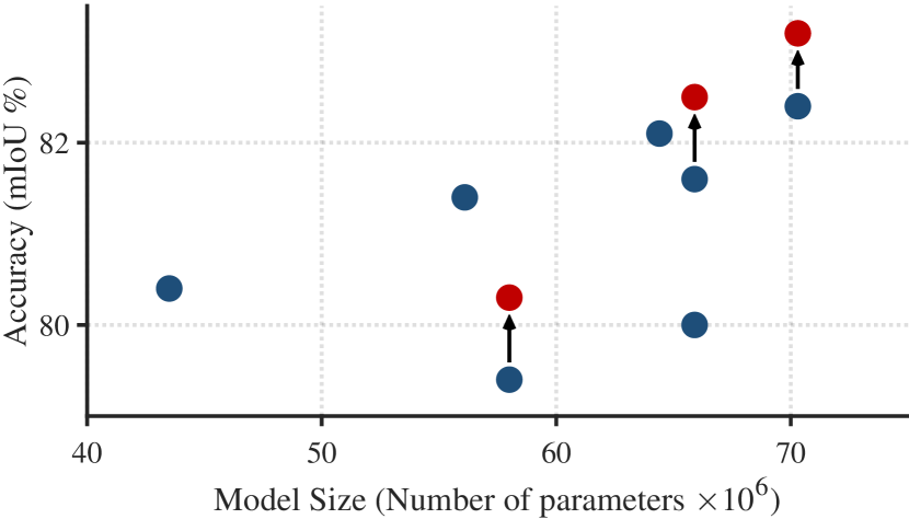
Figure 2: ​​​Accuracy ​vs. ​model ​size on Cityscapes ​test​ [15]. ​Our contrastive enables consistent performance improvements over state-of-the-arts, , DeepLabV3 ​[9], HRNet ​[64], OCR ​[79], without bringing any change to base networks during inference.

With our supervised pixel-wise contrastive algorithm, two novel techniques are developed. First, we propose a region memory bank to better address the nature of semantic segmentation. Faced with huge amounts of highly-structured pixel training samples, we let the memory store pooled features of semantic regions (, pixels with a same semantic label from a same image), instead of pixel-wise embeddings only. This leads to pixel-to-region contrast, as a complementary for the pixel-to-pixel contrast strategy. Such memory design allows us to access more representative data samples during each training step and fully explore structural relations between pixels and semantic-level segments, , pixels and segments belonging to a same class should be close in the embedding space. Second, we propose different sampling strategies to make better use of informative samples and let the segmentation model pay more attention to those segmentation-hard pixels. Previous works have confirmed that hard negatives are crucial for metric learning [37, 59, 61], and our study further reveals the importance of mining both informative negatives/positives and anchors in this supervised, dense image prediction task.

In a nutshell, our contributions are three-fold:

• We propose a supervised, pixel-wise contrastive learning method for semantic segmentation. It lifts current image-wise training strategy to an inter-image, pixel-to-pixel paradigm. It essentially learns a well structured pixel semantic embedding space, by making full use of the global semantic similarities among labeled pixels.

• We develop a region memory to better explore the large visual data space and support to further calculate pixel-to-region contrast. Integrated with pixel-to-pixel contrast computation, our method exploits semantic correlations among pixels, and between pixels and semantic regions.

• We demonstrate that more powerful segmentation models with better example and anchor sampling strategies could be delivered instead of selecting random pixel samples.

Our method can be seamlessly incorporated into existing segmentation networks without any changes to the base model and without extra inference burden during testing (Fig. 2). Hence, our method shows consistently improved intersection-over-union segmentation scores over challenging datasets (, Cityscapes​ [15], PASCAL-Context​ [52], COCO-Stuff​ [5] and CamVid​ [3]), using state-of-the-art segmentation architectures (, DeepLabV3​ [9], HRNet​ [64] and OCR​ [79]) and famous backbones (, ResNet​ [30], HRNet​ [64]). The impressive results shed light on the promises of metric learning in dense image prediction tasks. We expect this work to provide insights into the critical role of global pixel relationships in segmentation network training, and foster research on the open issues raised.

2 Related Work

Our work draws on existing literature in semantic segmentation, contrastive learning and deep metric learning. For brevity, only the most relevant works are discussed.

Semantic Segmentation. FCN [50] greatly promotes the advance of semantic segmentation. It is good at end-to-end dense feature learning, however, only perceiving limited visual context with local receptive fields. As strong dependencies exist among pixels in an image and these dependencies are informative about the structures of the objects [68], how to capture such dependencies becomes a vital issue for further improving FCN. A main group of follow-up effort attempts to aggregate multiple pixels to explicitly model context, for example, utilizing different sizes of convolutional/pooling kernels or dilation rates to gather multi-scale visual cues [78, 82, 8, 9], building image pyramids to extract context from multi-resolution inputs, adopting the Encoder-Decoder architecture to merge features from different network layers [57, 45], applying CRF to recover detailed structures [49, 85], and employing neural attention [65] to directly exchange context between paired pixels [10, 33, 34, 22]. Apart from investigating context-aggregation network modules, another line of work turns to designing context-aware optimization objectives [38, 2, 84], , directly verify segmentation structures during training, to replace the pixel-wise cross entropy loss.

Though impressive, these methods only address pixel dependencies within individual images, neglecting the global context of the labeled data, , pixel semantic correlations across different training images. Through a pixel-wise contrastive learning formulation, we map pixels in different categories to more distinctive features. The learned pixel features are not only discriminative for semantic classification within images, but also, more crucially, across images.

Contrastive Learning. Recently, the most compelling methods for learning representations without labels have been unsupervised contrastive learning [54, 32, 71, 13, 12], which significantly outperformed other pretext task-based alternatives [41, 24, 18, 53]. With a similar idea to exemplar learning [19], contrastive methods learn representations in a discriminative manner by contrasting similar (positive) data pairs against dissimilar (negative) pairs. A major branch of subsequent studies focuses on how to select the positive and negative pairs. For image data, the standard positive pair sampling strategy is to apply strong perturbations to create multiple views of each image data [71, 12, 29, 32, 6]. Negative pairs are usually randomly sampled, but some hard negative example mining strategies [39, 56, 36] were recently proposed. In addition, to store more negative samples during contrast computation, fixed [71] or momentum updated [51, 29] memories are adopted. Some latest studies [39, 31, 69] also confirm label information can assist contrastive learning based image-level pattern pre-training.

We raise a pixel-to-pixel contrastive learning method for semantic segmentation in the fully supervised setting. It yields a new training protocol that explores global pixel${}_{\!}$ relations in labeled data for regularizing segmentation embedding space. Though a few concurrent works also address contrastive learning in dense image prediction​ [73, 7, 67], the ideas are significantly different. First, they typically consider contrastive learning as a pre-training step for dense image embedding. Second, they simply use the local context within individual images, , only compute the contrast among pixels from augmented versions of a same image. Third, they do not notice the critical role of metric learning in complementing current well-established pixel-wise cross-entropy loss based training regime (cf.${}_{\!}$ §3.2).

Deep Metric Learning. The goal of metric learning is to quantify the similarity among samples using an optimal distance metric. Contrastive loss [26] and triplet loss [59] are two basic types of loss functions for deep metric learning. With a similar spirit of increasing and decreasing the distance between similar and dissimilar data samples, respectively, the former one takes pairs of sample as input while the latter is composed of triplets. Deep metric learning [20] has proven effective in a wide variety of computer vision tasks, such as image retrieval [63] and face recognition [59].

Although a few prior methods address the idea of metric learning in semantic segmentation, they only account for the local content from objects [27] or instances [16, 1, 20, 40]. It${}_{\!}$ is${}_{\!}$ worth${}_{\!}$ noting${}_{\!}$ [35]${}_{\!}$ also${}_{\!}$ explores${}_{\!}$ cross-image${}_{\!}$ information${}_{\!}$ of${}_{\!}$ training data, , leverage perceptual pixel groups for non-parametric pixel classification. Due to its clustering based metric learning strategy, [35] needs to retrieve extra labeled data for inference. Differently, our core idea, , exploit inter-image pixel-to-pixel similarity to enforce global constraints on the embedding space, is conceptually novel and rarely explored before. It is executed by a compact training paradigm, which enjoys the complementary advantages of unary, pixel-wise cross-entropy loss and pair-wise, pixel-to-pixel contrast loss, without bringing any extra inference cost or modification to the base network during deployment.

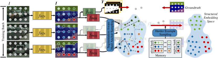
Figure 3: Detailed illustration of our pixel-wise contrastive learning based semantic segmentation network architecture.

3 Methodology

Before detailing our supervised pixel-wise contrastive algorithm for semantic segmentation (§3.2), we first introduce the contrastive formulation in unsupervised visual representation learning and the notion of memory bank (§3.1).

3.1 Preliminaries

Unsupervised Contrastive Learning. Unsupervised visual representation learning aims to learn a CNN encoder $f_{\text{CNN}}$ that transforms each training image $I$ to a feature vector $\bm{v}\!=\!f_{\text{CNN}}(I)\!\in\mathbb{R}^{D}$, such that $\bm{v}$ best describes $I$. To achieve this goal, contrastive approaches conduct training by distinguishing a positive (an augmented version of anchor $I$) from several negatives (images randomly drawn from the training set excluding $I$), based on the principle of similarity between samples. A popular loss function for contrastive learning, called InfoNCE [25, 54], takes the following form:​​​

$$\small\!\!\!\!\mathcal{L}^{\text{NCE}}_{I}\!=\!-\log\frac{\exp(\bm{v}\!\cdot\!\bm{v}^{+}/\tau)}{\exp(\bm{v}\!\cdot\!\bm{v}^{+}/\tau)\!+\!\sum_{\bm{v}^{-}\in\mathcal{N}_{I}}\exp(\bm{v}\!\cdot\!\bm{v}^{-}/\tau)},\!\!\vspace{-3pt}$$ (1)

where $\bm{v}^{+}$ is an embedding of a positive for $I$, $\mathcal{N}_{I}$ contains embeddings of negatives, ‘$\cdot$’ denotes the inner (dot) product, and $\tau\!>\!0$ is a temperature hyper-parameter. Note that all the embeddings in the loss function are $\ell_{2}$-normalized.

Memory Bank. As revealed by recent studies [71, 13, 29], a large set of negatives (, $|\mathcal{N}_{I}|$) is critical in unsupervised contrastive representation learning. As the number of negatives is limited by the mini-batch size, recent contrastive methods utilize large, external memories as a bank to store more navigate samples. Specifically, some methods [71] directly store the embeddings of all the training samples in the memory, however, easily suffering from asynchronous update. Some others choose to keep a queue of the last few batches [66, 13, 29] as memory. In [13, 29], the stored embeddings are even updated on-the-fly through a momentum-updated version of the encoder network $f_{\text{CNN}}$.

3.2 Supervised Contrastive Segmentation

Pixel-Wise Cross-Entropy Loss. In the context of semantic segmentation, each pixel $i$ of an image $I$ has to be classified into a semantic class $c\!\in\!\mathcal{C}$. Current approaches typically cast this task as a pixel-wise classification problem. Specifically, let $f_{\text{FCN\!}}$ be an FCN encoder (, ResNet [30]), that produces a dense feature $\bm{I}\!\in\!\mathbb{R}^{H\times W\times D\!}$ for $I$, from which the pixel embedding $\bm{i}\!\in\!\mathbb{R}^{D\!}$ of $i$ can be derived (, $\bm{i}\!\in\!\bm{I}$). Then a segmentation head $f_{\text{SEG\!}}$ maps $\bm{I}$ into a categorical score map $\bm{Y}\!=\!f_{\text{SEG\!}}(\bm{I})\!\in\!\mathbb{R}^{H\times W\times|\mathcal{C}|\!}$. Further let ${\bm{y}}\!=\![y_{1},\cdots\!,y_{|\mathcal{C}|}]\!\in\!\mathbb{R}^{|\mathcal{C}|\!}$ be the unnormalized score vector (termed as logit) for pixel $i$, derived from $\bm{Y}$, , ${\bm{y}}\!\in\!\bm{Y}$. Given ${\bm{y}}$ for pixel $i$ w.r.t its groundtruth label $\bar{c}\!\in\!\mathcal{C}$, the cross-entropy loss is optimized with softmax (cf. Fig. 3):​​

$$\small\mathcal{L}^{\text{CE}}_{i}=-\bm{1}^{\!\top}_{\bar{c}}\log(\texttt{softmax}({\bm{y}})),\vspace{-3pt}$$ (2)

where $\bm{1}_{\bar{c}}$ denotes the one-hot encoding of $\bar{c}$, the logarithm is defined as element-wise, and $\texttt{softmax}({y}_{c})\!=\!\frac{\exp({y}_{c})}{\sum_{c^{\prime}\!=\!1}^{|\mathcal{C}|}\exp(y_{c^{\prime}})}$. Such training objective design mainly suffers from two limitations. 1) It penalizes pixel-wise predictions independently but ignores relationship between pixels [84]. 2) Due to the use of softmax, the loss only depends on the relative relation among logits and cannot directly supervise on the learned representations [55]. These two issues were rarely noticed; only a few structure-aware losses are designed to address 1), by considering pixel affinity [38], optimizing intersection-over-union measurement [2], or maximizing the mutual information between the groundtruth and prediction map [84]. Nevertheless, these alternative losses only consider the dependencies between pixels within an image (, local context), regardless of the semantic correlations between pixels across images (, global structure).

Pixel-to-Pixel Contrast. In this work, we develop a pixel-wise contrastive learning method that addresses both 1) and 2), through regularizing the embedding space and exploring the global structures of training data. We first extend Eq. (1) to our supervised, dense image prediction setting. Basically, the data samples in our contrastive loss computation are training image pixels. In addition, for a pixel $i$ with its groundtruth semantic label $\bar{c}$, the positive samples are other pixels also belonging to the class $\bar{c}$, while the negatives are the pixels belonging to the other classes $\mathcal{C}\backslash\bar{c}$. Our supervised, pixel-wise contrastive loss is defined as:

$$\small\!\!\!\!\mathcal{L}^{\text{NCE}}_{i}\!=\!\frac{1}{|\mathcal{P}_{i}|}\!\!\sum_{\bm{i}^{+}\in\mathcal{P}_{i}\!\!}\!\!\!-_{\!}\log\frac{\exp(\bm{i}\!\cdot\!\bm{i}^{+\!\!}/\tau)}{\exp(\bm{i}\!\cdot\!\bm{i}^{+\!\!}/\tau)+\!\sum\nolimits_{\bm{i}^{-\!}\in\mathcal{N}_{i}\!}\!\exp(\bm{i}\!\cdot\!\bm{i}^{-\!\!}/\tau)},\!\!\vspace{-2pt}$$ (3)

where $\mathcal{P}_{i}$ and $\mathcal{N}_{i}$ denote pixel embedding collections of the positive and negative samples, respectively, for pixel $i$. Note that the positive/negative samples and the anchor $i$ are not restricted to being from a same image. As Eq. (3) shows, the purpose of such pixel-to-pixel contrast based loss design is to learn an embedding space, by pulling the same class pixel samples close and by pushing different class samples apart.

The pixel-wise cross-entropy loss in Eq. (2) and our contrastive loss in Eq. (3) are complementary to each other; the former lets segmentation networks learn discriminative pixel features that are meaningful for classification, while the latter helps to regularize the embedding space with improved intra-class compactness and inter-class separability through explicitly exploring global semantic relationships between pixel samples. Thus the overall training target is:

$$\small\mathcal{L}^{\text{SEG}}=\sum\nolimits_{i}\big{(}\mathcal{L}^{\text{CE}}_{i}+\lambda\mathcal{L}^{\text{NCE}}_{i}\big{)},\vspace{-1pt}$$ (4)

where $\lambda\!>\!0$ is the coefficient. As shown in Fig. ​4, the learned pixel embeddings by $\mathcal{L}^{\text{SEG}\!}$ become more compact and well separated. This suggests that, by enjoying the advantage of unary cross-entropy loss and pair-wise metric loss, segmentation network can generate more discriminative features, hence producing more promising results. Quantitative analyses are later provided in §4.2 and §4.3.

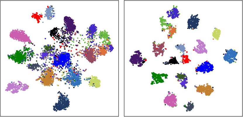
Figure 4: Visualization of features learned with (left) the pixel-wise entropy loss (, $\mathcal{L}^{\text{CE}}$ in Eq. (2)) and (right) our pixel contrast based optimization objective (, $\mathcal{L}^{\text{SEG}}$ in Eq. (4)) on Cityscapes val [15]. Features are colored according to class labels. As seen, the proposed $\mathcal{L}^{\text{SEG}}$ begets a well-structured semantic feature space.

Pixel-to-Region Contrast. As stated in §3.1, memory is a critical technique that helps contrastive learning to make use of massive data to learn good representations. However, since there are vast numbers of pixel samples in our dense prediction setting and most of them are redundant (, sampled from harmonious object regions), directly storing all the training pixel samples, like traditional memory [12], will greatly slow down the learning process. Maintaining several last batches in a queue, like [66, 13, 29], is also not a good choice, as recent batches only contain a limited number of images, reducing the diversity of pixel samples. Thus we choose to maintain a pixel queue per category. For each category, only a small number, , $V$, of pixels are randomly selected from each image in the latest mini-batch, and pulled into the queue, with a size of $T\!\gg\!V$. In practice we find this strategy is very efficient and effective, but the under-sampled pixel embeddings are too sparse to fully capture image content. Therefore, we further build a region memory bank that stores more representative embeddings absorbed from image segments (, semantic regions).

Specifically, for a segmentation dataset with a total of $N$ training images and $|\mathcal{C}|$ semantic classes, our region memory is built with size $|\mathcal{C}|\!\times\!N\!\times\!D$, where $D$ is the dimension of pixel embeddings. The $(\bar{c},n)$-th element in the region memory is a $D$-dimensional feature vector obtained by average pooling all the embeddings of pixels labeled as $\bar{c}$ category in the $n$-th image. The region memory brings two advantages: 1) store more representative “pixel” samples with low memory consumption; and 2) allow our pixel-wise contrastive loss (cf.${}_{\!}$ Eq.​ (3)) to further explore pixel-to-region relations. With regard to 2), when computing Eq.​ (3) for an anchor pixel $i$ belonging to $\bar{c}$ category, stored region embeddings with the same class $\bar{c}$ are viewed as positives, while the region embeddings with other classes $\mathcal{C}\backslash\bar{c}$ are negatives. For the pixel memory, the size is $|\mathcal{C}|\!\times\!T\!\times\!D$. Therefore, for the whole memory (denoted as $\mathcal{M}$), the total size is $|\mathcal{C}|\!\times\!(N\!+\!T)\!\times\!D$. We examine the design of $\mathcal{M}$ in §4.2. In the following sections, we will not distinguish pixel and region embeddings in $\mathcal{M}$, unless otherwise specified.

Hard Example Sampling. Prior research [59, 37, 39, 56, 36] found that, in addition to loss designs and the amount of training samples, the discriminating power of the training samples is crucial for metric learning. Considering our case, the gradient of the pixel-wise contrastive loss (cf. Eq. (3)) w.r.t. the anchor embedding $\bm{i}$ can be given as:

$$\small\!\!\frac{\partial\mathcal{L}^{\text{NCE}}_{i}}{\partial\bm{i}}\!=\!-_{\!}\frac{1}{\tau|\mathcal{P}_{i}|}\!\sum\nolimits_{\bm{i}^{+\!}\in\mathcal{P}_{i}\!\!\!}\Big{(}(1-p_{i^{+}\!})\cdot\bm{i}{{}^{+}\!}-\sum\nolimits_{\bm{i}^{-\!}\in\mathcal{N}_{i}\!}\!p_{i^{-}}\cdot\bm{i}^{-\!}\Big{)},\!\!$$ (5)

where $p_{i^{+\!/\!-\!\!}}\!\in\![0,1]$ denotes the matching probability between a positive/negative ${i}^{+\!/\!-\!}$ and the anchor ${i}$, , $p_{i^{+\!/\!-\!\!}}\!=\!\!\frac{\exp(\bm{i}\cdot\bm{i}^{+\!/\!-\!\!}/\tau)}{\sum_{\bm{i}^{\prime\!}\in\mathcal{P}_{\!i}\cup\mathcal{N}_{\!i}\!}\exp(\bm{i}\cdot\bm{i}^{\prime\!}/\tau)}$. We${}_{\!}$ view${}_{\!}$ the${}_{\!}$ negatives${}_{\!}$ with${}_{\!}$ dot${}_{\!}$ products${}_{\!}$ (, $\bm{i}\!\cdot\!\bm{i}^{-}$) closer${}_{\!}$ to${}_{\!}$ $1$${}_{\!}$ to${}_{\!}$ be${}_{\!}$ harder, , negatives which are similar to the anchor ${i}$. Similarly, the positives with dot products (, $\bm{i}\!\cdot\!\bm{i}^{+}$) closer to $-1$ are considered as harder, , positives${}_{\!}$ which${}_{\!}$ are${}_{\!}$ dissimilar${}_{\!}$ to${}_{\!}$ $i$.${}_{\!}$ We can find that, harder negatives bring more gradient contributions, , $p_{i^{-}}$, than easier negatives. This principle also holds true for positives, whose gradient contributions are $1_{\!}-_{\!}p_{i^{+}\!}$. Kalantidis et al. [36] further indicate that, as training progresses,${}_{\!}$ more${}_{\!}$ and${}_{\!}$ more${}_{\!}$ negatives${}_{\!}$ become${}_{\!}$ too simple to provide significant contributions to the unsupervised contrastive loss (cf.${}_{\!}$ Eq.​ (1)). This also happens in our supervised setting (cf.${}_{\!}$ Eq.​ (3)), for both negatives and positives. To remedy this problem, we propose the following sampling strategies:

• Hardest${}_{\!}$ Example${}_{\!}$ Sampling.${}_{\!}$ Inspired${}_{\!}$ by${}_{\!}$ hardest negative mining in metric learning [4], we first design a “hardest example sampling” strategy: for each anchor pixel embedding $\bm{i}$, only sampling top-$K$ hardest negatives and positives from the memory bank $\mathcal{M}$, for the computation of the pixel-wise contrastive loss (, $\mathcal{L}^{\text{NCE}}$ in Eq.​ (3)).

• Semi-Hard${}_{\!}$ Example${}_{\!}$ Sampling.${}_{\!}$ Some${}_{\!}$ studies${}_{\!}$ propose${}_{\!}$ to${}_{\!}$ make use of harder negatives, as${}_{\!}$ optimizing with${}_{\!}$ the${}_{\!}$ hardest negatives for metric learning likely leads to bad local minima [59, 72, 21]. Thus we further design a “semi-hard example sampling” strategy: for each anchor embedding $\bm{i}$, we first collect top $10\%$ nearest negatives (resp. top $10\%$ farthest positives) from the memory bank $\mathcal{M}$, from which we randomly then sample $K$ negatives (resp. $K$ positives) for our contrastive loss computation.

• Segmentation-Aware Hard Anchor Sampling. Rather than mining informative positive and negative examples, we develop an anchor sampling strategy. We treat the categorization ability of an anchor embedding as its importance during contrastive learning. This leads to “segmentation-aware hard anchor sampling”: the pixels with incorrect predictions, , $c\!\neq\!\bar{c}$, are treated as hard anchors. For the contrastive loss computation (cf. Eq.​ (3)), half of the anchors are randomly sampled and half are the hard ones. This anchor sampling strategy enables our contrastive learning to focus more on the pixels hard for classification, delivering more segmentation-aware embeddings.

In practice, we find “semi-hard example sampling” strategy performs better than “hardest example sampling”. In addition, after employing “segmentation-aware hard anchor sampling” strategy, the segmentation performance can be further improved. See §4.2 for related experiments.

3.3 Detailed Network Architecture

Our algorithm has five major components (cf. Fig.​ 3):

• FCN Encoder, $f_{\text{FCN}}$, which maps each input image $I$ into dense embeddings $\bm{I}\!=\!f_{\text{FCN}}(I)\!\in\!\mathbb{R}^{H\!\times\!W\!\times\!D}$. In our algorithm, any FCN backbones can be used to implement $f_{\text{FCN}}$ and we test two commonly used ones, , ResNet [30] and HRNet [64], in our experiments.

• Segmentation Head, $f_{\text{SEG}}$, that projects $\bm{I}$ into a score map $\bm{Y}\!\!=\!\!f_{\text{SEG}}(\bm{I})\!\in\!\mathbb{R}^{H\times\!W\!\times\!|\mathcal{C}|}$. We conduct evaluations using different segmentation heads in mainstream methods (, DeepLabV3 [9], HRNet [64], and OCR [79]).

• Project Head, $f_{\text{PROJ}}$, which maps each high-dimensional pixel embedding $\bm{i}\!\in\!\bm{I}$ into a 256-d $\ell_{2}$-normalized feature vector​ [12], for the computation of the contrastive loss $\mathcal{L}^{\text{NCE}}$. $f_{\text{PROJ}}$ is implemented as two $1\!\times 1\!$ convolutional layers with ReLU. Note that the project head is only applied during training and is removed at inference time. Thus it does not introduce any changes to the segmentation network or extra computational cost in deployment.

• Memory Bank, $\mathcal{M}$, which consists of two parts that store pixel and region embeddings, respectively. For each training image, we sample $V\!=\!10$ pixels per class. For each class, we set the size of the pixel queue as $T\!=\!10N$. The memory bank is also discarded after training.

• Joint Loss, $\mathcal{L}^{\text{SEG}\!}$ (cf. Eq. (4)), that takes the power of representation learning (, $\mathcal{L}^{\text{CE}}$ in Eq. (2)) and metric learning (, $\mathcal{L}^{\text{NCE}}$ in Eq. (3)) for more distinct segmentation feature learning. In practice, we find our method is not sensitive to the coefficient $\lambda$ (, when $\lambda\!\in\![0.1,1]$) and empirically set $\lambda$ as 1. For $\mathcal{L}^{\text{NCE}}$ in Eq. (3), we set the temperature $\tau$ as $0.1$. For sampling, we find “semi-hard example sampling” + “segmentation-aware hard anchor sampling” performs the best and set the numbers of sampled instances (, $K$) as $1,\!024$ and $2,\!048$ for positive and negative, respectively. For each mini-batch, 50 anchors are sampled per category (half are randomly sampled and the other half are segmentation-hard ones).

4 Experiment

4.1 Experimental Setup

Datasets. Our experiments are conducted on four datasets:​​

• Cityscapes [15] has $5,\!000$ finely annotated urban scene images, with $2,\!975/500/1,\!524$ for train/val/test. The segmentation performance is reported on $19$ challenging categories, such as person, sky, car, and building.

• PASCAL-Context [52] contains $4,\!998$ and $5,\!105$ images in train and test splits, respectively, with precise annotations of $59$ semantic categories.

• COCO-Stuff [5] consists of $10,\!000$ images gathered from COCO [46]. It is split into $9,\!000$ and $1,\!000$ images for train and test. It provides rich annotations for 80 object classes and 91 stuff classes.

• CamVid [3] has $367/101/233$ images for train/val/ test, with $11$ semantic labels in total.

Training. As mentioned in §3.3, various backbones (, ResNet​ [30] and HRNet​ [64]) and segmentation networks (, DeepLabV3​ [9], HRNet​ [64], and OCR​ [79]) are exploited in our experiments to thoroughly validate the proposed algorithm. We follow conventions [64, 79, 14, 74] for training hyper-parameters. For fairness, we initialize all backbones using corresponding weights pretrained on ImageNet [58], with the remaining layers being randomly initialized. For data augmentation, we use color jitter, horizontal flipping and random scaling with a factor in $[0.5,~{}2]$. We use SGD as our optimizer, with a momentum $0.9$ and weight decay $0.0005$. We adopt the polynomial annealing policy [9] to schedule the learning rate, which is multiplied by $(1\!-\!\frac{iter}{total\_iter})^{power\!}$ with $power\!=\!0.9$. Moreover, for Cityscapes, we use a mini-batch size of $8$, and an initial learning rate of $0.01$. All the training images are augmented by random cropping from $1024\!\times\!2048$ to $512\!\times\!1024$. For the experiments on test, we follow [64] to train the model for $100$K iterations. Note that we do not use any extra training data (, Cityscapes coarse [15]). For PASCAL-Context and COCO-Stuff, we opt a mini-batch size of $16$, an initial learning rate of $0.001$, and crop size of $520\!\times\!520$. We train for $60$K iterations over their train sets. For CamVid, we train the model for $6$K iterations, with batch size $16$, learning rate $0.02$ and original image size.

Testing. Following general protocol [64, 79, 60], we average the segmentation results over multiple scales with flipping, , the scaling factor is $0.75$ to $2.0$ (with intervals of $0.25$) times of the original image size. Note that, during testing, there is no any change or extra inference step introduced to the base segmentation models, , the projection head, $f_{\text{PROJ}}$, and memory bank, $\mathcal{M}$, are directly discarded.

Evaluation Metric. Following the standard setting, mean intersection-over-union (mIoU) is used for evaluation.

Reproducibility. Our model is implemented in PyTorch and trained on four NVIDIA Tesla V100 GPUs with a 32GB memory per-card. Testing is conducted on the same machine. Our implementations will be publicly released.

4.2 Diagnostic Experiment

We first study the efficacy of our core ideas and essential model designs, over Cityscapes val [15]. We adopt HRNet [64] as our base segmentation network (denoted as “Baseline (w/o contrast)” in Tables 1-3). To perform extensive ablation experiments, we train each model for $40$K iterations while keeping other hyper-parameters unchanged.

Pixel Contrast	Backbone	mIoU (%)
Baseline (w/o contrast)	HRNetV2-W48	78.1
Intra-Image Contrast	HRNetV2-W48	78.9 (+0.8)
Inter-Image Contrast	HRNetV2-W48	81.0 (+2.9)

Table 1: Comparison of different contrastive mechanisms on Cityscapes val [15]. See §4.2 for more details.

Memory	Backbone	mIoU (%)
Baseline (w/o contrast)	HRNetV2-W48	78.1
Mini-Batch (w/o memory)	HRNetV2-W48	79.8 (+1.7)
Pixel Memory	HRNetV2-W48	80.5 (+2.6)
Region Memory	HRNetV2-W48	80.2 (+2.1)
Pixel + Region Memory	HRNetV2-W48	81.0 (+2.9)

Table 2: Comparison of different memory bank designs on Cityscapes val [15]. See §4.2 for more details.

Inter-Image vs. ​Intra-Image Pixel Contrast. We first investigate the effectiveness of our core idea of inter-image pixel contrast. As shown in Table 1, additionally considering cross-image pixel semantic relations (, “Inter-Image Contrast”) in segmentation network learning leads to a substantial performance gain (, $\textbf{2.9}\%$), compared with “Baseline (w/o contrast)”. In addition, we develop another baseline, “Intra-Image Contrast”, which only samples pixels from same images during the contrastive loss (, $\mathcal{L}^{\text{NCE}}$ in Eq. (5)) computation. The results in Table 1 suggest that, although “Intra-Image Contrast” also boosts the performance over “Baseline (w/o contrast)” (, 78.1%$\rightarrow$78.9%), “Inter-Image Contrast” is more favored.

Sampling
Anchor	Pos./Neg.	Backbone	mIoU (%)
Baseline (w/o contrast)		HRNetV2-W48	78.1
	Random	HRNetV2-W48	79.3 (+1.2)
Random	Hardest	HRNetV2-W48	79.4 (+1.3)
	Semi-Hard	HRNetV2-W48	80.1 (+2.0)
Seg.-aware hard	Random	HRNetV2-W48	80.2 (+2.1)
	Hardest	HRNetV2-W48	80.5 (+2.4)
	Semi-Hard	HRNetV2-W48	81.0 (+2.9)

Table 3: Comparison of different hard example sampling strategies on Cityscapes val [15]. See §4.2 for more details.

Memory Bank. We next validate the design of our memory bank. The results are summarized in Table 2. Based on “Baseline (w/o contrast)”, we first derive a variant, “Mini-Batch w/o memory”: only compute pixel contrast within each mini-batch, without outside memory. It gets $79.8\%$ mIoU. We then provision this variant with pixel and region memories separately, and observe consistent performance gains ($79.8\%\!\rightarrow\!80.5\%$ for pixel memory and $79.8\%\!\rightarrow\!80.2\%$ for region memory). This evidences that i) leveraging more pixel samples during contrastive learning leads to better pixel embeddings; and ii) both pixel-to-pixel and pixel-to-region relations are informative cues. Finally, after using both the two memories, a higher score (, $81.0\%$) is achieved, revealing i) the effectiveness of our memory design; and ii) necessity of comprehensively considering both pixel-to-pixel contrast and pixel-to-region contrast.

Hard Example Mining. Table 3 presents a comprehensive examination of various hard example mining strategies proposed in §3.2. Our main observations are the following: i) For positive/negative sampling, mining meaningful pixels (, “hardest” or “semi-hard” sampling), rather than “random” sampling, is indeed useful; ii) Hence, “semi-hard” sampling is more favored, as it improves the robustness of training by avoiding overfitting outliers in the training set. This corroborates related observations in unsupervised setting [70] and indicates that segmentation may benefit from more intelligent sample treatment; and iii) For anchor sampling, “seg.-aware hard” strategy further improves the performance (, 80.1%$\rightarrow$81.0%) over “random” sampling only. This suggests that exploiting task-related signals in supervised metric learning may help develop better segmentation solutions, which has remained relatively untapped.

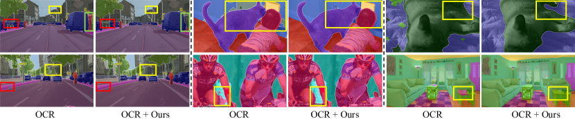
Figure 5: Visual comparisons between OCR [79] and OCR+Ours (from left to right: Cityscapes, PASCAL-Context, COCO-Stuff).

Model	Backbone	mIoU (%)
Model learned on Cityscapes train
PSPNet17 [82]	D-ResNet-101	78.4
PSANet18 [83]	D-ResNet-101	78.6
PAN18 [42]	D-ResNet-101	78.6
AAF18 [38]	D-ResNet-101	79.1
DeepLabV317 [9]	D-ResNet-101	78.1
DeepLabV3 $+~{}\textbf{{Ours}}$	D-ResNet-101	79.2 (+1.1)
HRNetV220 [64]	HRNetV2-W48	80.4
HRNetV2$+~{}\textbf{{Ours}}$	HRNetV2-W48	81.4 (+1.0)
Model learned on Cityscapes train+val
DFN18 [77]	D-ResNet-101	79.3
PSANet18 [83]	D-ResNet-101	80.1
SVCNet19 [17]	D-ResNet-101	81.0
CPN20 [75]	D-ResNet-101	81.3
DANet19 [22]	D-ResNet-101	81.5
ACF19 [80]	D-ResNet-101	81.8
DGCNet19 [81]	D-ResNet-101	82.0
HANet20 [14]	D-ResNet-101	82.1
ACNet19 [23]	D-ResNet-101	82.3
DeepLabV317 [9]	D-ResNet-101	79.4
DeepLabV3 $+~{}\textbf{{Ours}}$	D-ResNet-101	80.3 (+0.9)
HRNetV220 [64]	HRNetV2-W48	81.6
HRNetV2$+~{}\textbf{{Ours}}$	HRNetV2-W48	82.5 (+0.9)
OCR20 [79]	HRNetV2-W48	82.4
OCR$+~{}\textbf{{Ours}}$	HRNetV2-W48	83.2 (+0.8)

Table 4: Quantitative segmentation results on Cityscapes test [15]. D-ResNet-101 = Dilated ResNet-101. See §4.3.

4.3 Comparison to State-of-the-Arts

Cityscapes​ [15]. Table 4 lists the scores on Cityscapes test, under two widely used training settings [64] (trained over train or train+val). Our method brings impressive gains over 3 strong baselines (, DeepLabV3, HRNetV2, and OCR), and sets a new state-of-the-art.

Model	Backbone	mIoU (%)
DANet19 [22]	D-ResNet-101	52.6
SVCNet19 [17]	D-ResNet-101	53.2
CPN20 [75]	D-ResNet-101	53.9
ACNet19 [23]	D-ResNet-101	54.1
DMNet19 [28]	D-ResNet-101	54.4
RANet20 [60]	ResNet-101	54.9
DNL20 [74]	HRNetV2-W48	55.3
HRNetV220 [64]	HRNetV2-W48	54.0
HRNetV2$+~{}\textbf{{Ours}}$	HRNetV2-W48	55.1 (+1.1)
OCR20 [79]	HRNetV2-W48	56.2
OCR$+~{}\textbf{{Ours}}$	HRNetV2-W48	57.2 (+1.0)

Table 5: Quantitative segmentation results on PASCAL-Context test [52]. D-ResNet-101 = Dilated ResNet-101. See §4.3.

Model	Backbone	mIoU (%)
SVCNet19 [17]	D-ResNet-101	39.6
DANet19 [22]	D-ResNet-101	39.7
SpyGR20 [44]	ResNet-101	39.9
ACNet19 [23]	ResNet-101	40.1
HRNetV220 [64]	HRNetV2-W48	38.7
HRNetV2$+~{}\textbf{{Ours}}$	HRNetV2-W48	39.3 (+0.6)
OCR20 [79]	HRNetV2-W48	40.5
OCR$+~{}\textbf{{Ours}}$	HRNetV2-W48	41.0 (+0.5)

Table 6: Quantitative segmentation results on COCO-Stuff test [5]. D-ResNet-101 = Dilated ResNet-101. See §4.3.

Model	Backbone	mIoU (%)
DFANet19 [43]	Xception	64.7
BiSeNet18 [76]	D-ResNet-101	68.7
PSPNet17 [82]	D-ResNet-101	69.1
HRNetV220 [64]	HRNetV2-W48	78.5
HRNetV2$+~{}\textbf{{Ours}}$	HRNetV2-W48	79.0 (+0.5)
OCR20 [79]	HRNetV2-W48	80.1
OCR$+~{}\textbf{{Ours}}$	HRNetV2-W48	80.5 (+0.4)

Table 7: Quantitative segmentation results on CamVid test [3]. D-ResNet-101$=$Dilated ResNet-101. See §4.3.

PASCAL-Context [52]. Table 5 presents comparison results on PASCAL-Context test. Our approach improves the performance of base networks by solid margins (, $54.0\!\!\rightarrow\!\!55.1$ for HRNetV2, $56.2\!\!\rightarrow\!\!57.2$ for OCR). This is particularly impressive considering the fact that improvement on this extensively-benchmarked dataset is very hard.

COCO-Stuff [5]. Table 6 reports performance comparison of our method against seven competitors on COCO-Stuff test. As we find that OCR+Ours yields a mIoU of $41.0\%$, which leads to a promising gain of 0.5% over its counterpart (, OCR with a $40.5\%$ mIoU). Besides, HRNetV2+Ours outperforms HRNetV2 by 0.6%.

CamVid​ [3]. Table 7 shows that our method also leads to improvements over HRNetV2 and OCR on CamVid test.

Qualitative Results. fig:visual depicts qualitative comparisons of OCR+Ours against OCR over representative examples from three datasets (, Cityscapes, PASCAL-Context and COCO-Stuff). As seen, our method is capable of producing more accurate segments across various challenge scenarios.

5 Conclusion and Discussion

In${}_{\!}$ this${}_{\!}$ paper, we propose a${}_{\!}$ new${}_{\!}$ supervised${}_{\!}$ learning paradigm for semantic segmentation, enjoying the complementary advantages of unary classification and structured metric learning. Through pixel-wise contrastive learning, it investigates global semantic relations between training pixels, guiding pixel embeddings towards cross-image category-discriminative representations that eventually improve the segmentation performance. Our method generates promising results and shows great potential in a variety of dense image prediction tasks, such as pose estimation and medical image segmentation. It also comes with new challenges, in particular regarding smart data sampling, metric learning loss design, class rebalancing during training, and multi-layer feature contrast. Given the massive number of technique breakthroughs over the past few years, we expect a flurry of innovation towards these promising directions.

Loss	Type	Context	Backbone	mIoU (%)
Cross-Entropy Loss	unary	local	HRNetV2-W48	78.1
+AAF Loss [38]	pairwise	local	HRNetV2-W48	78.7
+RMI Loss [84]	higher-order	local	HRNetV2-W48	79.8
+Lovász Loss [2]	higher-order	local	HRNetV2-W48	80.3
+Contrastive Loss (Ours)	pairwise	global	HRNetV2-W48	81.0
+AAF [38] + Contrastive	-	-	HRNetV2-W48	81.0
+RMI [84] + Contrastive	-	-	HRNetV2-W48	81.3
+Lovász [2] + Contrastive	-	-	HRNetV2-W48	81.5

Table A1: Comparison of different loss designs on Cityscapes val [15]. See §A for more details.

Appendix A Comparison to Other Losses

We further study the effectiveness of our contrastive loss against representative semantic segmentation losses, including Cross-Entropy (CE) Loss, AAF loss [38], Lovász Loss [2], and RMI Loss [84].

For fair comparison, we examine each loss using HRNetV2 [64] as the base segmentation network, and train the loss jointly with CE on Cityscapes train for $40,\!000$ iterations with a mini-batch size of $8$. The results are reported in Table A1. We observe that all structure-aware losses outperform the standard CE loss. Notably, our contrastive loss achieves the best performance, outperforming the second-best Lovász loss by 0.7%, and the pairwise losses, , RMI and AAF, by 1.2% and 2.3%, respectively.

Additionally, Table A1 reports results of each loss in combination with our contrastive loss. From a perspective of metric learning, the CE loss can be viewed as a pixel-wise unary loss that penalizes each pixel independently and ignores dependencies between pixels, while AAF is a pairwise loss, which models the pairwise relations between spatially adjacent pixels. Moreover, the RMI and Lovász losses are higher-order losses: the former one accounts for region-level mutual information, and the latter one directly optimizes the intersection-over-union score over the pixel clique level. However, all these existing loss designs are defined within individual images, capturing local context/pixel relations only. Our contrastive loss, as it explores pairwise pixel-to-pixel dependencies, is also a pairwise loss. But it is computed over the whole training dataset, addressing the global context over the whole data space. Therefore, AAF can be viewed as a specific case of our contrastive loss, and additionally considering AAF does not bring any performance improvement. For other losses, our contrastive loss are complementary to them (global vs. local, pairwise vs. higher-order) and thus enables further performance uplifting. This suggests that designing a higher-order, global loss for semantic segmentation is a promising direction.

Appendix B Additional Quantitative Result

Table A2 provides comparison results with representative approaches on Cityscapes val [15] in terms of mIoU and training speed. We train our models on Cityscapes train for $80,\!000$ iterations with a mini-batch size of $8$. We find that, by equipping with cross-image pixel contrast, the performance of baseline models enjoy consistently improvements (1.2/1.1/0.8 points gain over DeepLabV3, HRNetV2 and OCR, respectively). In addition, the contrastive loss computation brings negligible training speed decrease, and does not incur any extra overhead during inference.

Model	Backbone	sec./iter.	mIoU (%)
SegSort19 [35]	D-ResNet-101	-	78.2
AAF18 [38]	D-ResNet-101	-	79.2
DeepLabV3+18 [11]	D-Xception-71	-	79.6
PSPNet17 [82]	D-ResNet-101	-	79.7
Auto-DeepLab-L19 [47]	-	-	80.3
HANet20 [14]	D-ResNet-101	-	80.3
SpyGR20 [44]	D-ResNet-101	-	80.5
ACF19 [80]	D-ResNet-101	-	81.5
DeepLabV317 [9]		1.18	78.5
DeepLabV3$+~{}\textbf{{Ours}}$	D-ResNet-101	1.37	79.7 (+1.2)
HRNetV220 [64]		1.67	81.1
HRNetV2$+~{}\textbf{{Ours}}$	HRNetV2-W48	1.87	82.2 (+1.1)
OCR20 [79]		1.29	80.6
OCR$+~{}\textbf{{Ours}}$	D-ResNet-101	1.41	81.2 (+0.6)
OCR20 [79]		1.75	81.6
OCR$+~{}\textbf{{Ours}}$	HRNetV2-W48	1.90	82.4 (+0.8)

Table A2: Quantitative semantic segmentation results on Cityscapes val​ [15]. D-ResNet-101 = Dilated-ResNet-101. D-Xception-71 = Dilated-Xception-71. See §B for more details.

Appendix C Additional Qualitative Result

We provide additional qualitative improvements of HRNetV2$+$Ours over HRNetV2 [64] on four benchmarks, including Cityscapes val [15] in fig:1, PASCAL-Context test [52] in fig:2, COCO-Stuff test [5] in fig:3, and CamVid test [3] in fig:4. The improved regions are marked by dashed boxes. As can be seen, our approach is able to produce great improvements on those hard regions, , small objects, cluttered background.

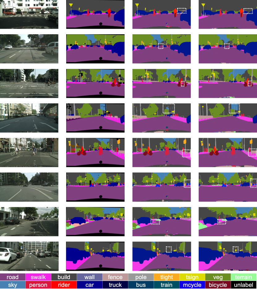
Figure A1: Qualitative semantic segmentation results on Cityscapes val [15]. From left to right: input images, ground-truths, results of HRNetV2 [64], results of HRNetV2$+$Ours. The improved regions are marked by white dashed boxes.

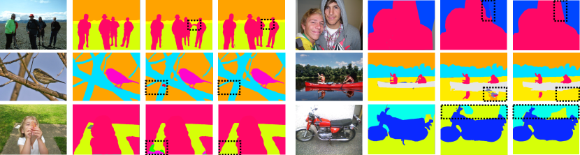
Figure A2: Qualitative semantic segmentation results on PASCAL-Context test [52]. From left to right: input images, ground-truths, results of HRNetV2 [64], results of HRNetV2$+$Ours. The improved regions are marked by black dashed boxes.

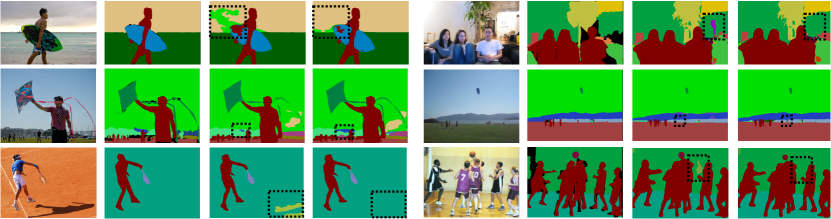
Figure A3: Qualitative semantic segmentation results on COCO-Stuff test [5]. From left to right: input images, ground-truths, results of HRNetV2 [64], results of HRNetV2$+$Ours. The improved regions are marked by black dashed boxes.

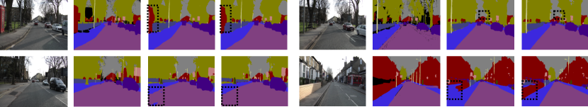
Figure A4: Qualitative semantic segmentation results on CamVid test [3]. From left to right: input images, ground-truths, results of HRNetV2 [64], results of HRNetV2$+$Ours. The improved regions are marked by black dashed boxes.

References

- [1] Min Bai and Raquel Urtasun. Deep watershed transform for instance segmentation. In CVPR, 2017.
- [2] Maxim Berman, Amal Rannen Triki, and Matthew B Blaschko. The lovász-softmax loss: A tractable surrogate for the optimization of the intersection-over-union measure in neural networks. In CVPR, 2018.
- [3] Gabriel J Brostow, Julien Fauqueur, and Roberto Cipolla. Semantic object classes in video: A high-definition ground truth database. Elsevier PRL, 30(2):88–97, 2009.
- [4] Maxime Bucher, Stéphane Herbin, and Frédéric Jurie. Hard negative mining for metric learning based zero-shot classification. In ECCV, 2016.
- [5] Holger Caesar, Jasper Uijlings, and Vittorio Ferrari. Coco-stuff: Thing and stuff classes in context. In CVPR, 2018.
- [6] Mathilde Caron, Ishan Misra, Julien Mairal, Priya Goyal, Piotr Bojanowski, and Armand Joulin. Unsupervised learning of visual features by contrasting cluster assignments. In NeurIPS, 2020.
- [7] Krishna Chaitanya, Ertunc Erdil, Neerav Karani, and Ender Konukoglu. Contrastive learning of global and local features for medical image segmentation with limited annotations. In NeurIPS, 2020.
- [8] Liang-Chieh Chen, George Papandreou, Iasonas Kokkinos, Kevin Murphy, and Alan L Yuille. Deeplab: Semantic image segmentation with deep convolutional nets, atrous convolution, and fully connected crfs. IEEE TPAMI, 40(4):834–848, 2017.
- [9] Liang-Chieh Chen, George Papandreou, Florian Schroff, and Hartwig Adam. Rethinking atrous convolution for semantic image segmentation. arXiv preprint arXiv:1706.05587, 2017.
- [10] Liang-Chieh Chen, Yi Yang, Jiang Wang, Wei Xu, and Alan L Yuille. Attention to scale: Scale-aware semantic image segmentation. In CVPR, 2016.
- [11] Liang-Chieh Chen, Yukun Zhu, George Papandreou, Florian Schroff, and Hartwig Adam. Encoder-decoder with atrous separable convolution for semantic image segmentation. In ECCV, 2018.
- [12] Ting Chen, Simon Kornblith, Mohammad Norouzi, and Geoffrey Hinton. A simple framework for contrastive learning of visual representations. In ICML, 2020.
- [13] Xinlei Chen, Haoqi Fan, Ross Girshick, and Kaiming He. Improved baselines with momentum contrastive learning. arXiv preprint arXiv:2003.04297, 2020.
- [14] Sungha Choi, Joanne T Kim, and Jaegul Choo. Cars can’t fly up in the sky: Improving urban-scene segmentation via height-driven attention networks. In CVPR, 2020.
- [15] Marius Cordts, Mohamed Omran, Sebastian Ramos, Timo Rehfeld, Markus Enzweiler, Rodrigo Benenson, Uwe Franke, Stefan Roth, and Bernt Schiele. The cityscapes dataset for semantic urban scene understanding. In CVPR, 2016.
- [16] Bert De Brabandere, Davy Neven, and Luc Van Gool. Semantic instance segmentation with a discriminative loss function. arXiv preprint arXiv:1708.02551, 2017.
- [17] Henghui Ding, Xudong Jiang, Bing Shuai, Ai Qun Liu, and Gang Wang. Semantic correlation promoted shape-variant context for segmentation. In CVPR, 2019.
- [18] Carl Doersch, Abhinav Gupta, and Alexei A Efros. Unsupervised visual representation learning by context prediction. In ICCV, 2015.
- [19] Alexey Dosovitskiy, Jost Tobias Springenberg, Martin Riedmiller, and Thomas Brox. Discriminative unsupervised feature learning with convolutional neural networks. In NeurIPS, 2014.
- [20] Alireza Fathi, Zbigniew Wojna, Vivek Rathod, Peng Wang, Hyun Oh Song, Sergio Guadarrama, and Kevin P Murphy. Semantic instance segmentation via deep metric learning. arXiv preprint arXiv:1703.10277, 2017.
- [21] Jonathan Frankle, David J Schwab, Ari S Morcos, et al. Are all negatives created equal in contrastive instance discrimination? arXiv preprint arXiv:2010.06682, 2020.
- [22] Jun Fu, Jing Liu, Haijie Tian, Yong Li, Yongjun Bao, Zhiwei Fang, and Hanqing Lu. Dual attention network for scene segmentation. In CVPR, 2019.
- [23] Jun Fu, Jing Liu, Yuhang Wang, Yong Li, Yongjun Bao, Jinhui Tang, and Hanqing Lu. Adaptive context network for scene parsing. In ICCV, 2019.
- [24] Spyros Gidaris, Praveer Singh, and Nikos Komodakis. Unsupervised representation learning by predicting image rotations. In ICLR, 2018.
- [25] Michael Gutmann and Aapo Hyvärinen. Noise-contrastive estimation: A new estimation principle for unnormalized statistical models. In AISTATS, 2010.
- [26] Raia Hadsell, Sumit Chopra, and Yann LeCun. Dimensionality reduction by learning an invariant mapping. In CVPR, 2006.
- [27] Adam W Harley, Konstantinos G Derpanis, and Iasonas Kokkinos. Segmentation-aware convolutional networks using local attention masks. In ICCV, 2017.
- [28] Junjun He, Zhongying Deng, and Yu Qiao. Dynamic multi-scale filters for semantic segmentation. In ICCV, 2019.
- [29] Kaiming He, Haoqi Fan, Yuxin Wu, Saining Xie, and Ross Girshick. Momentum contrast for unsupervised visual representation learning. In CVPR, 2020.
- [30] Kaiming He, Xiangyu Zhang, Shaoqing Ren, and Jian Sun. Deep residual learning for image recognition. In CVPR, 2016.
- [31] Olivier Henaff. Data-efficient image recognition with contrastive predictive coding. In ICML, 2020.
- [32] R Devon Hjelm, Alex Fedorov, Samuel Lavoie-Marchildon, Karan Grewal, Phil Bachman, Adam Trischler, and Yoshua Bengio. Learning deep representations by mutual information estimation and maximization. In ICLR, 2019.
- [33] Jie Hu, Li Shen, and Gang Sun. Squeeze-and-excitation networks. In CVPR, 2018.
- [34] Zilong Huang, Xinggang Wang, Lichao Huang, Chang Huang, Yunchao Wei, and Wenyu Liu. Ccnet: Criss-cross attention for semantic segmentation. In ICCV, 2019.
- [35] Jyh-Jing Hwang, Stella X Yu, Jianbo Shi, Maxwell D Collins, Tien-Ju Yang, Xiao Zhang, and Liang-Chieh Chen. Segsort: Segmentation by discriminative sorting of segments. In ICCV, 2019.
- [36] Yannis Kalantidis, Mert Bulent Sariyildiz, Noe Pion, Philippe Weinzaepfel, and Diane Larlus. Hard negative mixing for contrastive learning. In NeurIPS, 2020.
- [37] Mahmut Kaya and Hasan Şakir Bilge. Deep metric learning: A survey. Symmetry, 11(9):1066, 2019.
- [38] Tsung-Wei Ke, Jyh-Jing Hwang, Ziwei Liu, and Stella X Yu. Adaptive affinity fields for semantic segmentation. In ECCV, 2018.
- [39] Prannay Khosla, Piotr Teterwak, Chen Wang, Aaron Sarna, Yonglong Tian, Phillip Isola, Aaron Maschinot, Ce Liu, and Dilip Krishnan. Supervised contrastive learning. In NeurIPS, 2020.
- [40] Shu Kong and Charless Fowlkes. Recurrent pixel embedding for instance grouping. In CVPR, 2018.
- [41] Gustav Larsson, Michael Maire, and Gregory Shakhnarovich. Learning representations for automatic colorization. In ECCV, 2016.
- [42] Hanchao Li, Pengfei Xiong, Jie An, and Lingxue Wang. Pyramid attention network for semantic segmentation. arXiv preprint arXiv:1805.10180, 2018.
- [43] Hanchao Li, Pengfei Xiong, Haoqiang Fan, and Jian Sun. Dfanet: Deep feature aggregation for real-time semantic segmentation. In CVPR, 2019.
- [44] Xia Li, Yibo Yang, Qijie Zhao, Tiancheng Shen, Zhouchen Lin, and Hong Liu. Spatial pyramid based graph reasoning for semantic segmentation. In CVPR, 2020.
- [45] Guosheng Lin, Anton Milan, Chunhua Shen, and Ian Reid. Refinenet: Multi-path refinement networks for high-resolution semantic segmentation. In CVPR, 2017.
- [46] Tsung-Yi Lin, Michael Maire, Serge Belongie, James Hays, Pietro Perona, Deva Ramanan, Piotr Dollár, and C Lawrence Zitnick. Microsoft coco: Common objects in context. In ECCV, 2014.
- [47] Chenxi Liu, Liang-Chieh Chen, Florian Schroff, Hartwig Adam, Wei Hua, Alan L Yuille, and Li Fei-Fei. Auto-deeplab: Hierarchical neural architecture search for semantic image segmentation. In CVPR, 2019.
- [48] Weiyang Liu, Yandong Wen, Zhiding Yu, and Meng Yang. Large-margin softmax loss for convolutional neural networks. In ICML, 2016.
- [49] Ziwei Liu, Xiaoxiao Li, Ping Luo, Chen Change Loy, and Xiaoou Tang. Deep learning markov random field for semantic segmentation. IEEE TPAMI, 40(8):1814–1828, 2017.
- [50] Jonathan Long, Evan Shelhamer, and Trevor Darrell. Fully convolutional networks for semantic segmentation. In CVPR, 2015.
- [51] Ishan Misra and Laurens van der Maaten. Self-supervised learning of pretext-invariant representations. In CVPR, 2020.
- [52] Roozbeh Mottaghi, Xianjie Chen, Xiaobai Liu, Nam-Gyu Cho, Seong-Whan Lee, Sanja Fidler, Raquel Urtasun, and Alan Yuille. The role of context for object detection and semantic segmentation in the wild. In CVPR, 2014.
- [53] Mehdi Noroozi and Paolo Favaro. Unsupervised learning of visual representations by solving jigsaw puzzles. In ECCV, 2016.
- [54] Aaron van den Oord, Yazhe Li, and Oriol Vinyals. Representation learning with contrastive predictive coding. arXiv preprint arXiv:1807.03748, 2018.
- [55] Tianyu Pang, Kun Xu, Yinpeng Dong, Chao Du, Ning Chen, and Jun Zhu. Rethinking softmax cross-entropy loss for adversarial robustness. In ICLR, 2020.
- [56] Joshua Robinson, Ching-Yao Chuang, Suvrit Sra, and Stefanie Jegelka. Contrastive learning with hard negative samples. In ICLR, 2021.
- [57] Olaf Ronneberger, Philipp Fischer, and Thomas Brox. U-net: Convolutional networks for biomedical image segmentation. In MICCAI, 2015.
- [58] Olga Russakovsky, Jia Deng, Hao Su, Jonathan Krause, Sanjeev Satheesh, Sean Ma, Zhiheng Huang, Andrej Karpathy, Aditya Khosla, Michael S. Bernstein, Alexander C. Berg, and Fei-Fei Li. Imagenet large scale visual recognition challenge. IJCV, 115(3):211–252, 2015.
- [59] Florian Schroff, Dmitry Kalenichenko, and James Philbin. Facenet: A unified embedding for face recognition and clustering. In CVPR, 2015.
- [60] Dingguo Shen, Yuanfeng Ji, Ping Li, Yi Wang, and Di Lin. Ranet: Region attention network for semantic segmentation. NeurIPS, 2020.
- [61] Edgar Simo-Serra, Eduard Trulls, Luis Ferraz, Iasonas Kokkinos, Pascal Fua, and Francesc Moreno-Noguer. Discriminative learning of deep convolutional feature point descriptors. In ICCV, 2015.
- [62] Karen Simonyan and Andrew Zisserman. Very deep convolutional networks for large-scale image recognition. In ICLR, 2015.
- [63] Jiang Wang, Yang Song, Thomas Leung, Chuck Rosenberg, Jingbin Wang, James Philbin, Bo Chen, and Ying Wu. Learning fine-grained image similarity with deep ranking. In CVPR, 2014.
- [64] Jingdong Wang, Ke Sun, Tianheng Cheng, Borui Jiang, Chaorui Deng, Yang Zhao, Dong Liu, Yadong Mu, Mingkui Tan, Xinggang Wang, et al. Deep high-resolution representation learning for visual recognition. IEEE TPAMI, 2020.
- [65] Xiaolong Wang, Ross Girshick, Abhinav Gupta, and Kaiming He. Non-local neural networks. In CVPR, 2018.
- [66] Xun Wang, Haozhi Zhang, Weilin Huang, and Matthew R Scott. Cross-batch memory for embedding learning. In CVPR, 2020.
- [67] Xinlong Wang, Rufeng Zhang, Chunhua Shen, Tao Kong, and Lei Li. Dense contrastive learning for self-supervised visual pre-training. In CVPR, 2021.
- [68] Zhou Wang, Alan C Bovik, Hamid R Sheikh, and Eero P Simoncelli. Image quality assessment: from error visibility to structural similarity. IEEE TIP, 13(4):600–612, 2004.
- [69] Longhui Wei, Lingxi Xie, Jianzhong He, Jianlong Chang, Xiaopeng Zhang, Wengang Zhou, Houqiang Li, and Qi Tian. Can semantic labels assist self-supervised visual representation learning? arXiv preprint arXiv:2011.08621, 2020.
- [70] Mike Wu, Chengxu Zhuang, Milan Mosse, Daniel Yamins, and Noah Goodman. On mutual information in contrastive learning for visual representations. arXiv preprint arXiv:2005.13149, 2020.
- [71] Zhirong Wu, Yuanjun Xiong, Stella X Yu, and Dahua Lin. Unsupervised feature learning via non-parametric instance discrimination. In CVPR, 2018.
- [72] Jiahao Xie, Xiaohang Zhan, Ziwei Liu, Yew Soon Ong, and Chen Change Loy. Delving into inter-image invariance for unsupervised visual representations. arXiv preprint arXiv:2008.11702, 2020.
- [73] Zhenda Xie, Yutong Lin, Zheng Zhang, Yue Cao, Stephen Lin, and Han Hu. Propagate yourself: Exploring pixel-level consistency for unsupervised visual representation learning. arXiv preprint arXiv:2011.10043, 2020.
- [74] Minghao Yin, Zhuliang Yao, Yue Cao, Xiu Li, Zheng Zhang, Stephen Lin, and Han Hu. Disentangled non-local neural networks. In ECCV, 2020.
- [75] Changqian Yu, Jingbo Wang, Changxin Gao, Gang Yu, Chunhua Shen, and Nong Sang. Context prior for scene segmentation. In CVPR, 2020.
- [76] Changqian Yu, Jingbo Wang, Chao Peng, Changxin Gao, Gang Yu, and Nong Sang. Bisenet: Bilateral segmentation network for real-time semantic segmentation. In ECCV, 2018.
- [77] Changqian Yu, Jingbo Wang, Chao Peng, Changxin Gao, Gang Yu, and Nong Sang. Learning a discriminative feature network for semantic segmentation. In CVPR, 2018.
- [78] Fisher Yu and Vladlen Koltun. Multi-scale context aggregation by dilated convolutions. In ICLR, 2016.
- [79] Yuhui Yuan, Xilin Chen, and Jingdong Wang. Object-contextual representations for semantic segmentation. In ECCV, 2020.
- [80] Fan Zhang, Yanqin Chen, Zhihang Li, Zhibin Hong, Jingtuo Liu, Feifei Ma, Junyu Han, and Errui Ding. Acfnet: Attentional class feature network for semantic segmentation. In ICCV, 2019.
- [81] Li Zhang, Xiangtai Li, Anurag Arnab, Kuiyuan Yang, Yunhai Tong, and Philip HS Torr. Dual graph convolutional network for semantic segmentation. In BMVC, 2019.
- [82] Hengshuang Zhao, Jianping Shi, Xiaojuan Qi, Xiaogang Wang, and Jiaya Jia. Pyramid scene parsing network. In CVPR, 2017.
- [83] Hengshuang Zhao, Yi Zhang, Shu Liu, Jianping Shi, Chen Change Loy, Dahua Lin, and Jiaya Jia. Psanet: Point-wise spatial attention network for scene parsing. In ECCV, 2018.
- [84] Shuai Zhao, Yang Wang, Zheng Yang, and Deng Cai. Region mutual information loss for semantic segmentation. In NeurIPS, 2019.
- [85] Shuai Zheng, Sadeep Jayasumana, Bernardino Romera-Paredes, Vibhav Vineet, Zhizhong Su, Dalong Du, Chang Huang, and Philip HS Torr. Conditional random fields as recurrent neural networks. In ICCV, 2015.