A Bayesian approach for estimation of weight matrices in spatial autoregressive models††thanks: This working paper is an earlier draft of an article published by Taylor & Francis in Spatial Economic Analysis on 22nd July 2022, available at: https://www.tandfonline.com/doi/full/10.1080/17421772.2022.2095426.
Abstract
We develop a Bayesian approach to estimate weight matrices in spatial autoregressive (or spatial lag) models. Datasets in regional economic literature are typically characterized by a limited number of time periods relative to spatial units . When the spatial weight matrix is subject to estimation severe problems of over-parametrization are likely. To make estimation feasible, our approach focusses on spatial weight matrices which are binary prior to row-standardization. We discuss the use of hierarchical priors which impose sparsity in the spatial weight matrix. Monte Carlo simulations show that these priors perform very well where the number of unknown parameters is large relative to the observations. The virtues of our approach are demonstrated using global data from the early phase of the COVID-19 pandemic.
Keywords: Estimation of spatial weight matrix, spatial econometric model, Bayesian MCMC estimation, Monte Carlo simulations, COVID-19 pandemic
JEL Codes: C11, C21, C23, C51
1 Introduction
Spatial econometrics deals with the study of cross-sectional dependence and interactions among (spatial) observations. A particularly popular spatial econometric model is the spatial autoregressive (or spatial lag) specification, where spatial interdependence between observations is governed by a so-called spatial weight matrix. The spatial weight matrix is typically assumed non-negative, row-standardized and exogenously given, with spatial weights based on some concept of neighbourhood. Geographic neighbourhood is often preferred due to exogeneity assumptions. However, when relying on geographic information, several competing approaches exist for constructing the weight matrix (for a thorough discussion, see LeSage and Pace 2009). Recently, Kelejian and Piras (2014), Qu and Lee (2015), Han and Lee (2016), and Hsieh and Lee (2016) use alternative measures, such as (socio-)economic proximity. Another strand of the literature focusses on the uncertainty associated with the choice of neighbourhood structures by selecting or combining alternative weight matrices (see, for example, Debarsy and LeSage 2018 and Piribauer and Cuaresma 2016).
Since direct estimation of a spatial weight matrix requires estimating at least parameters (ignoring the other model parameters), only few approaches target direct estimation of spatial weight matrices. Recently, Ahrens and Bhattacharjee (2015) and Lam and Souza (2020) tackle this problem through LASSO-based approaches (Tibshirani 1996), which involve (a priori) expert knowledge about the interactions between spatial units, while allowing the final estimates of the spatial weights to slightly deviate from it.111Ahrens and Bhattacharjee (2015) consider the case of sparsity in the spatial weights by employing shrinkage towards the zero matrix. However, for regional economic panels, where the time dimension is often limited relative to the number of spatial observations , estimation results in a deleterious proliferation of the number of parameters.
In this paper we describe a novel and flexible Bayesian approach for estimation of spatial weight matrices. Our definition of spatial weight matrices fulfils the typical assumptions employed in the vast majority of spatial econometric literature. The resulting spatial weight matrices are assumed non-negative and specific requirements to identification of the parameters can be easily implemented in a Markov-chain Monte Carlo (MCMC) sampling strategy. Although our primary focus is on row-standardized spatial weight matrices, weights without row-standardization are also implementable. To make our estimation approach applicable to spatial panels where the number of time periods is limited as compared to the number of spatial units , we focus on spatial weight matrices which are binary prior to potential row-standardization.
In this paper we primarily focus on scenarios where no a priori information on the spatial structure is available. However, we also discuss how a priori spatial information can be implemented in a very simple and transparent way. For cases where the number of unknown parameters is large relative to the number of observations, we discuss hierarchical prior setups which impose sparsity in the weight matrix. In a Monte Carlo study, we show that these sparsity priors perform particularly well when the number of spatial observations is large relative to the time periods .
We show that our approach can be implemented in an efficient Gibbs sampling algorithm, which implies that the estimation strategy can be easily extended to other spatial econometric specifications. Among several others, such extensions include shrinkage estimation to avoid overparameterization (Piribauer and Cuaresma 2016), more flexible specifications of the innovation process (LeSage 1997), controlling for unobserved spatial heterogeneity (Cornwall and Parent 2017; Piribauer 2016), or allowing for non-linearity in the slope parameters (Basile 2008; Krisztin 2017). It is moreover worth noting that the proposed approach can be easily adapted to matrix exponential spatial specifications (LeSage and Pace 2007), spatial error specifications (see, LeSage and Pace 2009), or local spillover models (Vega and Elhorst 2015).
The rest of the paper is organized as follows: the next section outlines the panel version of the considered spatial lag model. Section 3 discusses the Bayesian estimation approach of the spatial weights along with several potential prior setups. Section 4 presents the Bayesian MCMC estimation algorithm and also discusses how to efficiently deal with the computational difficulties when updating the spatial weights in the MCMC sampler. Section 5 assesses the accuracy of the sampling procedure via a Monte Carlo simulation study. Section 6 illustrates our approach using data on global infection rates of the very first phase of the recent COVID-19 pandemic. The final section concludes.
2 Econometric framework
We consider a panel version of a global spillover spatial autoregressive model (SAR) of the form:222We also consider specifications with a spatial lag of the temporally lagged dependent variable. Sampling strategies for these cases are presented in the appendix.
| (1) |
where denotes an vector of observations on the dependent variable measured at period . and represent parameters associated with fixed effects for the spatial units and time periods, respectively. is an full rank matrix of explanatory variables, with corresponding vector of slope parameters . is a standard disturbance term .
The matrix denotes a spatial weight matrix and is a (scalar) spatial dependence parameter. is non-negative with if observation is considered as a neighbour to , and otherwise. A vital assumption is also that , in order to avoid the case that an observation is assumed as a neighbour to itself. A frequently made assumption amongst practitioners is that is row-stochastic with rows summing to unity. In this paper, we mainly present results relating to row-stochastic weight matrices. However, as the decision on row-standardizing depends on the empirical application, it is worth noting that the proposed approach may be easily adapted to problems without row-standardization of .333Thorough discussions on the implications of row-standardization are provided by Plümper and Neumayer (2010) and Liu et al. (2014).
The reduced form of the SAR model is given by:
| (2) |
where is a so-called spatial multiplier matrix. To ensure that () is invertible, appropriate stability conditions need to be imposed. For row-stochastic spatial weight matrices, a sufficient stability condition for the spatial autoregressive parameter often employed is (see, for example, LeSage and Pace 2009).
In most cases, the elements of are typically treated as known. In the spatial econometric literature, there are various ways as a means to constructing such a spatial weight matrix. In this study we focus on estimation of weight matrices which are binary prior to row-standardization. We therefore assume that the typical element of our spatial weight matrix can be obtained from an unknown spatial adjacency matrix (with typical element ).444Eq. (3) implies some observations may have zero neighbours. However, priors on the number of neighbours can be easily elicited to rule out such situations. Moreover, a researcher might easily abstain from row-standardization by neglecting the transformation in Eq. (3). We therefore define , where denotes the row-standardization function:555The function may simply be dropped when considering models without row-standardization of .
| (3) |
The elements of the adjacency matrix are assumed as unknown binary indicators, which are subject to estimation. It is worth noting that the assumption of a binary covers a wide range of specifications commonly used in the literature such as contiguity, distance band, or nearest neighbours (see, for example, LeSage and Pace 2009).
To alleviate further notation, we collect the respective dummy variables associated with the fixed effects along with the explanatory variables in a matrix with corresponding parameter vector . Moreover, define , , , and denotes the data. The Gaussian likelihood is then given by:
| (4) |
When the elements of the spatial weight matrix are subject to estimation, the number of unknown parameters is likely much larger than the number of observations. Since spatial economic panels often feature limited relative to , the proposed estimation approach has to address the issue of over-parametrization. We discuss different ways to tackle this problem. First and foremost, one may reduce the dimensionality of the problem by imposing a priori information on spatial weights or assuming symmetry of the spatial neighbourhood structure. Alternatively, we consider hierarchical prior setups which impose sparsity in the weight matrix.
When estimating spatial weights in addition to the spatial and slope parameters, identification issues are more complicated as compared to models assuming exogenous spatial weights. We therefore follow De Paula et al. (2019), who provide a thorough discussion on parameter identification for rather general spatial autoregressive model specifications. As mentioned before, we consider spatial weight matrices which are non-negative and for all . Further standard assumptions include , , and for some positive , as well as . As an additional identifying assumption, it is important that the main diagonal elements of are not proportional to a vector of ones.666The most obvious case, where this assumption would be violated is a fully connected with for all . Sufficient conditions for global identification are fulfilled if we make the additional assumption of (see Corollary 3 in De Paula et al. 2019). Without this additional restriction on , De Paula et al. (2019) show that a strongly connected spatial network for global identification is needed. Since strong a priori information on the spatial weight matrix is often not available (or desired), we therefore assume and only consider positive spatial autocorrelation, which is a typical assumption for empirical applications.777These assumptions can be checked during estimation by using standard rejection sampling techniques in the MCMC sampling steps (see, for example, LeSage and Pace 2009, or Koop 2003). Rejection sampling rejects draws of parameter combinations which do not fulfil these assumptions.
3 Bayesian estimation of W
In this paper we use a Bayesian estimation approach to obtain estimates and inference on the unknown quantities , , , as well as the elements of . After eliciting suitable priors for the unknown parameters, we employ a computationally efficient MCMC algorithm.
Let denote the prior belief in including the th element of the spatial weight matrix. Conversely, for a proper prior specification the prior probability of exclusion is then simply given by . With denoting the elements of the neighbourhood matrix without , the posterior probabilities of and conditional on all other parameters are given by:
| (5) |
where and are given by through updating the spatial weight matrix via setting and , respectively.888To reduce the dimensionality of the parameter space, an interesting alternative might be the assumption of a symmetric , which halves the number of free elements in the spatial weight matrix. This assumption can be imposed in the way by simply simultaneously updating , respectively. Using the law of total probability, it is straightforward to show that the resulting conditional posterior for is Bernoulli:
| (6) |
with and given in Eq. (5). Since the conditional posterior follows a convenient and well-known form, efficient Gibbs sampling can be employed.
A Bayesian estimation framework requires elicitation of a prior on . Obvious candidates are independent Bernoulli priors on the unknown indicators :
| (7) |
where denotes the prior inclusion probability of , . Conversely, the prior probability of exclusion then simply takes the form .
A natural prior choice would involve setting for , and zero otherwise, which implies that each off-diagonal element in has an equal prior chance of being included. However, in many cases a researcher has possible a priori information on the underlying structure of the spatial weight matrix. The following stylized examples demonstrate how to incorporate such information in a flexible and straightforward way.
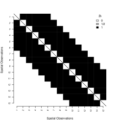
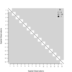
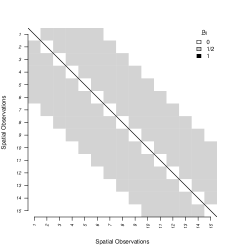
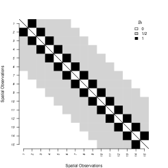
Notes: Alternative prior setups for a linear city of spatial observations. Case (A) shows a prior specification without any prior uncertainty on the spatial links. This setup implies an exogenous and no estimation of the weights is involved. Case (B) involves no spatial prior information and each element has a prior probability of inclusion . Case (C) shows uncertainty of the linkages in only within a certain spatial domain. Case (D) is a stylized prior specification considering uncertainty among two (or more) weight matrices, with setting in regions where the two matrices overlap.
Figure 1 illustrates the flexibility of prior elicitation for in the case of a "linear city" with equidistant regions. Case (A) in the figure shows a prior specification without any prior uncertainty on the elements of by setting if and are considered as neighbours and zero otherwise. In this case, no estimation on the spatial links is involved and the model reduces to a standard SAR model with an exogenously given (in this example, a distance band specification).
Case (B) depicts the opposite case where no prior spatial information is available. Specifically, this case considers full estimation of all potential links with respective prior inclusion probability for .
Subplots (C) and (D) in Figure 1 depict prior setups where a priori spatial information is available to the researcher, but associated with uncertainty. Case (C) illustrates a prior where the general spatial domain is assumed as being a priori known, but uncertainty over specific linkages exists. In empirical practice, spatial weight matrices based on geographic information are often viewed as being preferable due to exogeneity assumptions to (socio-)economic data. The illustrated prior specification follows this idea by still allowing for uncertainty and flexibility among the spatial neighbourhood.
Recent contributions to spatial econometric literature propose selecting (Piribauer and Cuaresma 2016) or combining (Debarsy and LeSage 2018) multiple exogenous spatial weight matrices. Case (D) follows a similar idea by depicting a mixture of a distance band and a contiguity matrix (i.e. neighbourhood if regions share a common border). The intersecting elements of the two spatial structures (resulting in a contiguity matrix) are assumed as being included by setting .
Hierarchical prior setups and sparsity
The prior structure in Eq. (7) involves fixed inclusion probabilities , which implies that the number of neighbours of observation follows a Binomial distribution with a prior expected number of neighbours of . However, such a prior structure has the potential undesirable effect of promoting a relatively large number of neighbours. For example, when , the prior expected number of neighbours is , since combinations of resulting in such a neighbourhood size are dominant in number.
To put more prior weight on parsimonious neighbourhood structures and therefore promote sparsity in the adjacency matrix, one may explicitly account for the number of linkages in each row of the adjacency matrix . We consider a flexible prior structure on the number of neighbours that corresponds to a beta-binomial distribution with two prior hyperparameters . The beta-binomial distribution is the result of treating the prior inclusion probability as random (rather than being fixed) by placing a hierarchical beta prior on it. For , the resulting prior can be written as follows:
| (8) |
where denotes the Gamma function, and and are prior hyperparameters.
In the case of , the prior takes the form of a discrete uniform distribution over the number of neighbours. By fixing , we follow Ley and Steel (2009) and anchor the prior expected number of neighbours via .
4 Bayesian MCMC estimation of the model
This section presents the Bayesian MCMC estimation algorithm for the proposed modelling framework. Estimation is carried out using an efficient Gibbs sampling scheme. The only exception is the sampling step for the spatial (scalar) autoregressive parameter , where we propose using a standard griddy Gibbs step.999A random walk Metropolis-Hastings step for might be employed as an alternative. The sampling scheme involves the following steps:
-
I.
Set starting values for the parameters (e.g. by sampling from the prior distributions)
-
II.
Sequentially update the parameters by subsequently sampling from the conditional posterior distributions presented in this section.
Step II. is repeated for times after discarding the first draws as burn-ins.
Sampling and
For the slope parameters and the error variance we use common Normal and inverted Gamma prior specifications, respectively. Specifically, and ), where , , and denote prior hyperparameters.
The resulting conditional posterior distribution is Gaussian and of well-known form (see, for example, LeSage and Pace 2009):
| (9) | |||||
The conditional posterior of is inverted Gamma:
| (10) | |||||
Sampling
For the spatial parameter , we use a standard Beta distribution (see LeSage and Pace, 2009, p. 142). The conditional posterior is given by:
| (11) |
Note that the conditional posterior for does not follow a well-known form and thus requires alternative sampling techniques. We follow LeSage and Pace (2009) and use a griddy-Gibbs step (Ritter and Tanner 1992) to sample .101010Since the support for is limited, the griddy-Gibbs approach (or sometimes inversion approach) relies on univariate numerical integration techniques of the conditional posterior for and uses the cumulative density function for producing draws of . A Metropolis-Hastings step may be used as a standard alternative, but these typically produce less efficient draws with poorer mixing properties (see also LeSage and Pace 2009).
Sampling the elements of the adjacency matrix
As discussed in the previous section, we propose two alternative prior specifications for the unknown indicators of the spatial weight matrix First, an independent Bernoulli prior structure with fixed inclusion probabilities (7). Second, a hierarchical prior structure which treats the inclusion probabilities as random (8). After eliciting the prior, the binary indicators can be sequentially sampled in random order from a Bernoulli distribution with conditional posterior given in (6).
Fast computation of the determinant terms
For the Bayesian MCMC algorithm, it is worth noting that repeated sampling from Eq. (6) is required. However, this requires evaluating the conditional probabilities and in Eq. (5). The main computational difficulty lies in the calculation of the determinants and , which has to be carried out per Gibbs sampling step for the unknown elements of the spatial adjacency matrix. The computational costs associated with direct calculation of these determinants steeply rises with – in fact by a factor of . This makes direct evaluation of the determinant prohibitively expensive, especially for large values of . To avoid direct evaluation, we provide computationally efficient updates for the determinant, allowing for estimation of models with larger sample sizes.
It is worth noting that it is not necessary to directly calculate the determinant of the matrix (with ). Only the determinant of the matrix needs to be updated, since . Here, denotes the spatial weight matrix obtained by setting and , respectively.
Direct evaluation of can be largely avoided, since updating changes only the -th row of , if we do not restrict to be symmetric (we will address this case shortly). To illustrate, let denote the current – to be updated – spatial adjacency matrix, and the associated spatial weight matrix with determinant . Using the so-called matrix determinant lemma, we can efficiently calculate:
| (12) |
is an vector of zeros, except for its -th entry, which is unity. The vector contains the differences between the -th row of and the -th row of .
It becomes clear that Eq. (12) provides a computationally cheap way for updating the determinant , conditional on and . This implies that during the MCMC procedure, for each update of , we have to keep track of the determinant (for which Eq. (12) provides a simple update) and the inverse of . Direct evaluation of is – similar to direct evaluation of the determinant – prohibitively expensive for moderate to large , since it has to be carried out for each unknown element of . However, we can rely on the so-called Sherman-Morrison formula to avoid direct evaluation of the matrix inverse:
| (13) |
Combining the formulas in Eqs. (12) and (13) thus provides a numerically cheap and viable way to update the elements of the spatial adjacency matrix.111111Note the implication that an update of necessitates a direct evaluation of the determinant and the matrix inverse , as in this case no convenient equations exist. An update of , however, has to be performed only once per Gibbs step, as opposed to the updates necessary for , thus justifying the relatively higher computational costs.
The binary nature of can be exploited for additional computational gains. Either or always exactly equals and thus its determinant and inverse is already known. This only necessitates calculating and for only or for , but not both.
If a symmetric spatial adjacency matrix is assumed, the update process remains generally the same, however the determinant and matrix inverse updates have to be performed iteratively. In this case, both and (for ) are set to either or . Thus, both the -th and the -th row of differ from . Following the notation in the non-symmetric case, let us denote the differences between these rows as and . To obtain an update of and , we first evaluate Eqs. (12) and (13), based on , , , and . Using the resulting determinant and matrix inverse, as well as , and , we again evaluate Eqs. (12) and (13), which yield and .
5 Simulation study
To assess the accuracy of our proposed approach, we evaluate its performance in a Monte Carlo study. Our benchmark data generating process comprises two randomly generated explanatory variables, as well as spatial unit and time fixed effects:
To maintain succinct notation, we denote the simulated values in the Monte Carlo study with a tilde. The matrix of explanatory variables is defined as , where both and are normally distributed with zero mean and variance of one, . The corresponding vector of coefficients is defined as . The vector of residuals is generated from a normal distribution with zero mean and . The fixed effects parameters and are randomly generated from a standard normal distribution.
The row-stochastic spatial weight matrix is based on an adjacency matrix , which is generated from an nearest neighbour specification, by additionally assuming symmetry of the weight matrix prior to row-standardization.121212More specifically, where is a nearest neighbour adjacency matrix. The nearest neighbour specification is based on a randomly generated spatial location pattern, sampled from a normal distribution with zero mean and unity variance. In the Monte Carlo study we vary and . Additionally, we vary the strength of spatial dependence .
For the Monte Carlo simulation study, we compare the following prior setups:
-
1.
Fixed () prior: this prior corresponds to the fixed Bernoulli prior specification in Eq. (7), where we set .
-
2.
Sparsity () prior: this is analogous to the prior setup in Eq. (8), with . This prior setup corresponds to a discrete uniform distribution over the number of neighbours.
-
3.
Sparsity () prior: this prior setup corresponds to Eq. (8), with and . We set the number of a priori expected neighbours to . This prior setup thus imposes more sparsity in as compared to the former.
For all prior specifications under scrutiny, we consider two alternative estimation setups by assuming that the adjacency matrix is either symmetric or non-symmetric.131313However, a direct comparison of the results between symmetric and non-symmetric specifications does not appear reasonable, since the adjacency matrix in the data generating process is assumed symmetric. We moreover report the predictive performance of two alternative specifications using exogenous weight matrices. In these cases the employed weights are based on the true (symmetric) adjacency matrix by fixing the accuracy to the 99% and 95% level, respectively. We simulate such cases by randomly switching 1% and 5% of the elements in the true binary adjacency matrix , respectively. The resulting exogenous adjacency matrices thus result in exactly 99% and 95% overlap in the binary observations with the true adjacency matrix, while maintaining the same level of sparsity.
The prior setup for our remaining parameters is as follows. We assume a Gaussian prior for with zero mean and a variance of . We use an inverse gamma prior for with rate and shape parameters . The prior for the spatial autoregressive parameter is a symmetric Beta specification with shape and rate parameters equal to . The chosen priors can thus be considered highly non-informative.
In Table 1 we use several criteria to evaluate the performance of the alternative specifications. For the spatial autoregressive and the slope parameters we report the well-known root mean squared error (RMSE). For assessing the ability to estimating the spatial adjacency matrix, we use the measure of accuracy. The accuracy measure is defined as the sum of correctly identified unknown elements, divided by the number of total elements to be estimated. This measure is calculated separately for each posterior draw. The reported value is an average over all posterior draws and Monte Carlo iterations.
[tbp] Non-symmetric Symmetric Exogenous Fixed Sparsity Sparsity Fixed Sparsity Sparsity RMSE() 20 40 0.3 0.193 0.161 0.163 0.162 0.163 0.164 0.168 0.176 0.5 0.172 0.173 0.172 0.170 0.169 0.171 0.179 0.216 0.8\bigstrut[b] 0.169 0.169 0.169 0.165 0.166 0.167 0.287 0.553 10 0.3 0.234 0.207 0.198 0.203 0.182 0.181 0.192 0.204 0.5 0.257 0.210 0.206 0.189 0.191 0.190 0.206 0.253 0.8\bigstrut[b] 0.217 0.216 0.217 0.205 0.204 0.206 0.371 0.658 100 40 0.3 0.098 0.099 0.097 0.099 0.099 0.098 0.079 0.080 0.5 0.144 0.088 0.083 0.145 0.114 0.076 0.084 0.086 0.8\bigstrut[b] 0.154 0.087 0.088 0.073 0.081 0.081 0.089 0.141 10 0.3 0.111 0.112 0.111 0.111 0.111 0.112 0.092 0.093 0.5 0.135 0.118 0.104 0.135 0.136 0.118 0.088 0.094 0.8\bigstrut[b] 0.346 0.143 0.140 0.254 0.102 0.102 0.100 0.151 RMSE() 20 40 0.3 0.199 0.029 0.031 0.030 0.029 0.030 0.034 0.060 0.5 0.035 0.040 0.042 0.035 0.035 0.035 0.039 0.083 0.8\bigstrut[b] 0.021 0.021 0.022 0.018 0.018 0.018 0.084 0.177 10 0.3 0.237 0.152 0.094 0.291 0.147 0.106 0.058 0.080 0.5 0.155 0.060 0.054 0.109 0.053 0.051 0.059 0.114 0.8\bigstrut[b] 0.027 0.032 0.032 0.028 0.028 0.029 0.097 0.179 100 40 0.3 0.280 0.283 0.277 0.279 0.283 0.287 0.027 0.033 0.5 0.447 0.109 0.101 0.446 0.353 0.220 0.021 0.054 0.8\bigstrut[b] 0.148 0.044 0.047 0.049 0.024 0.024 0.034 0.097 10 0.3 0.242 0.256 0.268 0.245 0.252 0.274 0.050 0.062 0.5 0.373 0.176 0.141 0.371 0.391 0.404 0.041 0.074 0.8\bigstrut[b] 0.473 0.106 0.110 0.169 0.141 0.137 0.044 0.105 Accuracy 20 40 0.3 0.648 0.930 0.954 0.963 0.982 0.983 0.990 0.950 0.5 0.983 0.988 0.989 0.998 0.998 0.998 0.990 0.950 0.8\bigstrut[b] 0.995 0.995 0.995 0.999 1.000 0.999 0.990 0.950 10 0.3 0.554 0.752 0.866 0.679 0.875 0.904 0.990 0.950 0.5 0.734 0.898 0.931 0.915 0.962 0.967 0.990 0.950 0.8\bigstrut[b] 0.975 0.983 0.984 0.996 0.997 0.997 0.990 0.950 100 40 0.3 0.530 0.713 0.847 0.539 0.686 0.848 0.990 0.950 0.5 0.530 0.898 0.929 0.539 0.793 0.933 0.990 0.950 0.8\bigstrut[b] 0.847 0.966 0.966 0.978 0.977 0.977 0.990 0.950 10 0.3 0.530 0.713 0.844 0.539 0.685 0.846 0.990 0.950 0.5 0.530 0.746 0.883 0.539 0.702 0.905 0.990 0.950 0.8\bigstrut[b] 0.531 0.926 0.933 0.564 0.944 0.944 0.990 0.950
-
•
Notes: Results are based on Monte Carlo iterations. For each Monte Carlo iteration the corresponding sampling algorithms are run using draws, where the initial were discarded as burn-in. The values given for RMSE() and RMSE() correspond to the average root mean squared error over all Monte Carlo iterations. Bold values denote the best performing specification within a section (symmetric or non-symmetric). The exogenous specifications correspond to classic SAR models with randomly perturbed exogenous adjacency matrices, which have an accuracy of 99% and 95% compared to the true adjacency matrix. For RMSEs, lower values indicate outperformance. Conversely, for the accuracy indicators of , higher values indicate outperformance.
Table 1 summarizes the results of our Monte Carlo simulation. For all combinations of , , under scrutiny, the table presents the respective root mean square error for both the slope coefficients and the spatial autoregressive parameter. The third block of the table shows the accuracy of the estimated adjacency matrix . Lower values in terms of RMSEs indicate outperformance. Conversely, for accuracy in higher values indicate outperformance. The best performance among the three employed prior scenarios within a subgroup is highlighted in bold. In addition, the last two columns in Table 1 show the results for the benchmark SAR models using exogenous randomly perturbed adjacency matrices with accuracy fixed at the and the level, respectively.
Intuitively, the precision of the estimation improves as the number of observations increases in proportion to the number of unknown parameters.141414The number of unknown parameters amounts to and for non-symmetric and symmetric spatial weight matrices, respectively. The results in Table 1 largely confirm this intuition. The performance indicators for both and also clearly improve for high levels of spatial autocorrelation (). In scenarios where the number of unknown parameters is smaller than the number of observations our approach even manages to outperform both rather hard benchmarks using exogenous spatial weight matrices close to the true DGP. This relative outperformance appears particularly pronounced when the strength of spatial dependence is large. In these settings, symmetric specifications (which resemble the true DGP) even manage to produce accuracy in the adjacency matrix close to unity.
Particularly interesting results appear in the most challenging Monte Carlo scenarios, where the number of unknown parameters is particularly large relative to the number of observations ( and ). In these scenarios, the number of parameters to be estimated exceeds the number of observations by a factor of more than ten. In these cases, prior specifications without using shrinkage appear to fail estimating the underlying spatial structure by producing rather poor accuracy measures. However, when employing sparsity priors, the table reveals that our approach still manages to produce relatively accurate predictive results. In the existence of pronounced spatial autocorrelation, the sparsity specifications even manage to closely track the predictive performance of the rather tough exogenous benchmarks.
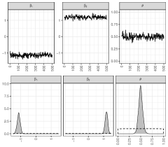
Note that the symmetric specifications (where we impose ) typically outperform their non-symmetric counterparts due to their resemblance to the true DGP. However, for settings where the number of unknown parameters is smaller than the number of observations both scenarios track each other closely. Among the alternative prior specifications under scrutiny, the table shows rather similar results (no clear best specification emerges) in scenarios where is small relative to . However, for particularly over-parametrized settings (high and low ) the proposed sparsity priors particularly outperform the fixed setups. Specifically, even in the scenario with and , the sparsity priors still perform comparatively well.151515Figure A4 in the appendix illustrates the convergence properties of a random Monte Carlo sample for the case of and . This case was chosen as it is similar to the settings in the empirical applications.
6 Empirical illustration
To illustrate our proposed approach using real data, we estimate spatial panel specifications based on country-specific daily infection rates in the very early phase of the coronavirus pandemic. We use the COVID-19 data set provided by the Johns Hopkins University (Dong et al. 2020). The database contains information on (official) daily infections for a large panel of countries around the globe. For the empirical illustration, we focus on the very beginning of the outbreak by using data from 17th of February to the 20th of April of 2020.
The starting date of our sample marks the beginning of the pandemic in major countries, such that large parts of Asia, Europe and North America can be included.161616Countries without any (official) infections in the starting period have been excluded from the sample. We moreover exclude India as a clear outlier from the sample due to its particular small (official) infection rates throughout the observation period. The choice of the end date is motivated by the results of Krisztin et al. (2020), where the degree of spatial dependence among infections rates becomes insignificant after the 20th April, when the majority of countries in the sample implemented lockdown policies.
For the empirical application we use data for the following countries: Australia (AUS), Bahrain (BHR), Belgium (BEL), Canada (CAN), China (CHN), Finland (FIN), France (FRA), Germany (DEU), Iran (IRN), Iraq (IRQ), Israel (ISR), Italy (ITA), Japan (JPN), Kuwait (KWT), Lebanon (LBN), Malaysia (MYS), Oman (OMN), Republic of Korea (KOR), Russian Federation (RUS), Singapore (SGP), Spain (ESP), Sweden (SWE), Thailand (THA), United Arab Emirates (ARE), United Kingdom (GBR), United States (USA), and Viet Nam (VNM).
By including a biweekly time lag, our resulting panel thus comprises countries across the globe for a period of days.171717With a biweekly time lag, the dependent variable thus captures data from 2nd of April to the 20th of April (). For a better comparison, we have fixed the time period captured by for all alternative specifications. It is moreover worth noting that a notable earlier starting date would result in relatively few (cross-sectional) observations. However, our results, are rather robust when considering a longer time horizon. We follow work by Guliyev (2020), Krisztin et al. (2020), or Han et al. (2021), among others, and use panel versions of a spatial growth specification for the country-specific COVID-19 infections:
| (14) |
where , and is an vector comprising the (logged) daily number of official cases per 100,000 inhabitants per country for time period .181818The spatial growth regression in (14) may be alternatively specified in levels rather than in log-differences by setting . Results using this alternative specification are very similar and are presented in the appendix. and represent fixed effects for the countries and the time periods, respectively. denotes the spatial weight matrix with spatial autoregressive parameter as defined before. We again primarily focus on row-stochastic weight matrices. Results based on spatial weight matrices without row-standardization are presented in the appendix.
We also consider alternative model specifications using contemporaneous as well as temporal lags of the spatial lag ( with ). A plethora of recent studies exploit the contemporaneous spatial information () for modelling the spread of COVID-19 infections (among others, see Han et al. 2021, Jaya and Folmer 2021, Kosfeld et al. 2021, Guliyev 2020, or Krisztin et al. 2020). Using contemporaneous spatial information appears reasonable when the primary interest lies in quantifying spatial co-movements of infection rates. However, for many questions of interest, a temporal spatial lag () might be an interesting alternative since it reflects the notion that the spatial process of virus transmission takes some time to manifest (Elhorst 2021, Mitze and Kosfeld 2021). Since our proposed estimation approach can be easily applied to these alternative specifications, we provide estimates for both specifications.191919It is worth noting that in the special case of , computational efficiency is tremendously increased, as no log-determinant calculations are required in the MCMC algorithm. The sampling strategy for these cases is presented in the appendix.
In addition to the Initial infections variable , matrix contains three explanatory variables on a daily basis. Several studies emphasize the importance of climatic condition on the COVID-19 virus spread. For a survey on the effects of climate on the spread of the COVID-19 pandemic, see Briz-Redón and Serrano-Aroca (2020). We therefore use daily data on the country specific maximum measured temperature (Temperature) and precipitation levels (Precipitation) as additional covariates. Both variables stem from a daily database of country-specifc data, which was compiled via the Dark Sky API.202020https://www.kaggle.com/datasets/vishalvjoseph/weather-dataset-for-covid19-predictions As a third variable, we also include the well-known stringency index (Stringency) put forward by Hale et al. (2020), which summarizes country-specific governmental policy measures to contain the spread of the virus. In this application, we use the biweekly average of the reported stringency index. Since all these influences arguably require some time to be reflected in the official infection figures, we use a biweekly lag of days (in accordance with in alternative variants).212121As robustness checks, we have also tried a shorter lag length of one week. The estimated spatial structures appeared very similar to the biweekly benchmarks. All these additional robustness checks, along with the R codes, are available from the authors upon request.
[tbp]
| Fixed | Sparsity | Fixed | Sparsity | |||||
| Mean | Std.Dev. | Mean | Std.Dev. | Mean | Std.Dev. | Mean | Std.Dev. | |
| Initial infections | -0.8761 | 0.0117 | -0.9244 | 0.0117 | -0.9533 | 0.0126 | -0.9911 | 0.0114 |
| Stringency | -0.4566 | 0.0736 | -0.5661 | 0.0451 | -0.2503 | 0.0858 | 0.0616 | 0.0410 |
| Precipitation | 0.0365 | 0.0339 | -0.0444 | 0.0335 | 0.0541 | 0.0608 | 0.0483 | 0.0511 |
| Temperature | -0.0014 | 0.0015 | -0.0016 | 0.0015 | -0.0032 | 0.0026 | -0.0017 | 0.0025 |
| 0.6319 | 0.0129 | 0.5592 | 0.0101 | 0.9618 | 0.0110 | 0.9481 | 0.0139 | |
| 0.0187 | 0.0013 | 0.0209 | 0.0014 | 0.0401 | 0.0034 | 0.0516 | 0.0036 | |
| Avg. # neighbours | 7.8370 | 3.6083 | 4.2849 | 2.8082 | ||||
| Fixed effects | Yes | Yes | Yes | Yes | ||||
| 27 | 27 | 27 | 27 | |||||
| 19 | 19 | 19 | 19 | |||||
-
•
Notes: Posterior quantities based on MCMC draws, where the first were discarded as burn-ins. Values in bold denote significance under a 90% posterior credible interval.
Table 2 presents a summary of the estimation results. The left part of the table shows results for specifications using a contemporaneous spatial lag , while the right part summarizes results for the case .
For each specification, the first rows contain the posterior mean and standard deviations for the slope parameters followed by estimates of and . Posterior quantities which appear significantly different from zero using a 90% posterior credible interval are depicted in bold. The table moreover presents the average posterior expected number of neighbours, which is given by the average row sum of the matrix of posterior inclusion probabilities based on . This measure can be viewed as a measure of sparsity in the estimated matrix of linkages. All specifications moreover contain fixed effects for both and .222222For the benchmark specifications, the number of unknown parameters and observations thus amounts to and , respectively.
Table 2 shows rather similar and posterior quantities for the flat and the sparsity prior. However, there appear some marked differences between the specifications and . In all cases, spatial dependence appears strong and precisely estimated, but appears particularly high in the temporal lag specification . However, the table similarly reveals higher estimates for the nuisance parameter for the temporal spatial lag models. The table shows rather precise and negative coefficients for the initial infections variable, indicating conditional convergence patterns. For most model variants the table moreover suggests a significant negative impact of the stringency index on infection growth. The majority of the slope parameter estimates associated with the variables temperature and precipitation appear more muted and insignificant. Overall, the table moreover clearly demonstrates that a hierarchical prior setup can enforce sparsity in the resulting adjacency matrix. Both sparsity specifications result in an average number of neighbours smaller than the models with fixed prior specifications.
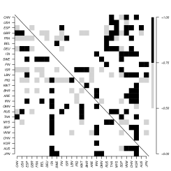
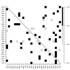
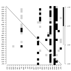

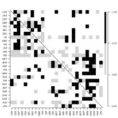
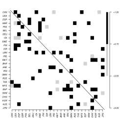
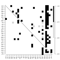
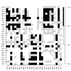
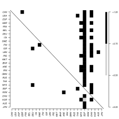
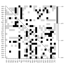
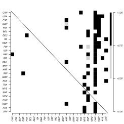
Notes: Posterior inclusion probabilities of spatial links based on MCMC draws. Inclusion probabilities 0.50-0.75 (little evidence for inclusion) are coloured grey. Strong evidence for inclusion (>0.75) indicated by black colour.
Figure 2 depicts the posterior inclusion probabilities for the considered specifications. To better visualize the results we have reordered the countries by their longitudes, starting with Canada and the United States and ending with south-east Asian countries, Australia and Japan. Clusters along the main diagonal thus roughly indicate geographic spatial linkages. For the sake of visualization, we distinguish between negligible evidence for inclusion (; white colour), moderate evidence (; grey colour), and strong evidence (; black colour).
The two upper plots in Figure 2 depict posterior inclusion probabilities for the specifications involving a contemporaneous spatial lag , while the lower part shows temporal spatial lag specifications . In both cases, the left subplots present results based on independent prior inclusion probabilities of . The right plots are based on sparsity priors using . The columns in the subplots indicate marginal posterior importance of the countries as predictors of coronavirus infections in linked countries. Conversely, rows depict the countries to be predicted. The results using sparsity priors generally produce similar patterns as the fixed prior specifications and clearly demonstrate its ability of dimension reduction in the connectivity structure. For the contemporaneous spatial lag specification (upper plots), the figure suggests a slightly more pronounced regional dependency structure as compared to the temporal spatial lags. The figure moreover reveals marked spill-out effects from Asian countries, as well as from Iran and Italy.232323The regional dependency structure appears particularly pronounced when a level specification of the infection dynamics is imposed. Sensitivity checks based on this alternative specifications are presented in Figure A1 in the appendix.
Results based on a biweekly temporal spatial lag show even more pronounced spill-out effects from Asian countries (most notably China, Republic of Korea, and Singapore).242424When comparing the results, it is important to note that for all specifications under scrutiny, we have fixed time period in the dependent variable ( ranges from the 2nd February to the 20th of February; i.e. ).The biweekly temporal spatial lag specification thus inherently comprises spatial information prior to the period in . For European countries, results similarly suggest Italy as a further important source country of spatial virus transmission. The estimated spatial linkages are thus in close agreement with the actual origins of the overall virus transmission for the very early period of the global outbreak of the pandemic.
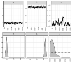
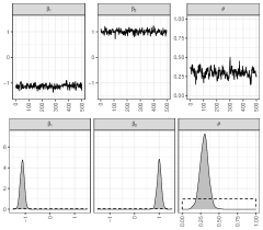
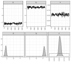
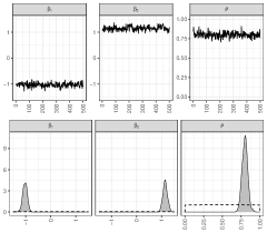
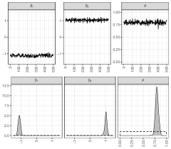
To showcase convergence of the posterior MCMC chains, Figure 3 depicts trace plots for , , and slope parameters. Overall, the trace plots show rather good mixing and convergence properties. Convergence of the chains have moreover been checked using the diagnostics proposed by Geweke (1992) implemented in the R package coda (Plummer et al. 2006). Results moreover appear rather robust concerning alternative modelling frameworks. Estimation results of these alternative specifications are presented in the appendix.252525Estimates when using a smaller time lag of seven days also appear very similar. Results along with the R codes used are available from the authors upon request.
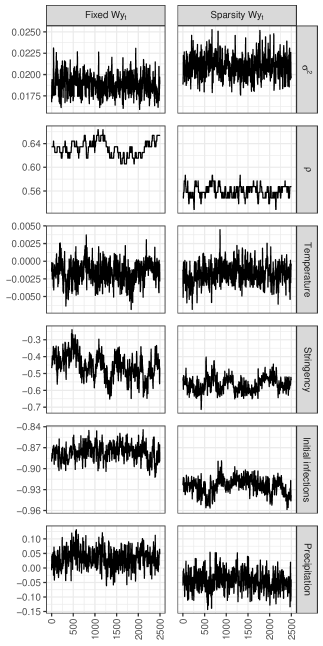
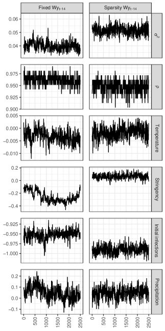
Notes: Posterior draws based on MCMC draws, where the first were discarded as burn-ins.
7 Concluding remarks
In this paper we propose a Bayesian approach for estimation of weight matrices in spatial econometric models. A particular advantage of our approach is the simple integration into a standard Bayesian MCMC algorithm. The proposed framework can therefore be adapted and extended in a simple and computationally efficient way to cover a large number of alternative spatial specifications prevalent in recent literature. Our approach may thus be easily extended to cover inter alia non-Gaussian models such as spatial probit (LeSage et al., 2011) or logit specifications (Krisztin and Piribauer, 2021), local spillover models (Vega and Elhorst, 2015), or spatial error models (LeSage and Pace, 2009).
Our approach does not not necessarily rely on specific prior information for the spatial linkages. Spatial information, however, can be easily implemented in a flexible and transparent way. We moreover motivate the use of hierarchical priors which impose sparsity in the resulting spatial weight matrix. These sparsity priors are particularly useful in applications where the number of unknown parameters exceeds those of the observations. The virtues of our approach comes at the price that we focus on spatial neighbourhood structures which are binary (prior to row-standardization). However, this assumption is implicitly assumed in many spatial applications in the regional economic literature where spatial weight matrices are constructed based on concepts of contiguity, distance band, or nearest neighbours.
Based on Monte Carlo simulations, we show that our approach appears particularly promising when the number of spatial observations is large relative to the time dimension , which is a rather common characteristic of data sets in the regional science literature. We moreover demonstrate the usefulness of our approach using real data on the outbreak of the COVID-19 pandemic. The results of this empirical application corroborate the findings in the Monte Carlo simulation study that the proposed approach performs well even in the cases of high over-parametrization.
References
- Ahrens and Bhattacharjee (2015) Ahrens A and Bhattacharjee A (2015) Two-step lasso estimation of the spatial weights matrix. Econometrics 3(1), 128–155
- Basile (2008) Basile R (2008) Regional economic growth in Europe: A semiparametric spatial dependence approach. Papers in Regional Science 87(4), 527–544
- Briz-Redón and Serrano-Aroca (2020) Briz-Redón Á and Serrano-Aroca Á (2020) The effect of climate on the spread of the COVID-19 pandemic: A review of findings, and statistical and modelling techniques. Progress in Physical Geography: Earth and Environment 44(5), 591–604
- Cornwall and Parent (2017) Cornwall GJ and Parent O (2017) Embracing heterogeneity: the spatial autoregressive mixture model. Regional Science and Urban Economics 64, 148–161
- De Paula et al. (2019) De Paula Á, Rasul I and Souza P (2019) Identifying network ties from panel data: theory and an application to tax competition. arXiv preprint arXiv:1910.07452
- Debarsy and LeSage (2018) Debarsy N and LeSage J (2018) Flexible dependence modeling using convex combinations of different types of connectivity structures. Regional Science and Urban Economics 69, 48–68
- Dong et al. (2020) Dong E, Du H and Gardner L (2020) An interactive web-based dashboard to track COVID-19 in real time. The Lancet infectious diseases 20(5), 533–534
- Elhorst (2021) Elhorst JP (2021) The dynamic general nesting spatial econometric model for spatial panels with common factors: Further raising the bar. Review of Regional Research , 1–19
- Geweke (1992) Geweke J (1992) Evaluating the accuracy of sampling-based approaches to the calculations of posterior moments. Bayesian Statistics 4, 641–649
- Guliyev (2020) Guliyev H (2020) Determining the spatial effects of COVID-19 using the spatial panel data model. Spatial Statistics 38, 100443
- Hale et al. (2020) Hale T, Petherick A, Phillips T and Webster S (2020) Variation in government responses to COVID-19. Blavatnik School of Government Working Paper 31, 2020–11
- Han and Lee (2016) Han X and Lee LF (2016) Bayesian analysis of spatial panel autoregressive models with time-varying endogenous spatial weight matrices, common factors, and random coefficients. Journal of Business & Economic Statistics 34(4), 642–660
- Han et al. (2021) Han X, Xu Y, Fan L, Huang Y, Xu M and Gao S (2021) Quantifying COVID-19 importation risk in a dynamic network of domestic cities and international countries. Proceedings of the National Academy of Sciences 118(31)
- Hsieh and Lee (2016) Hsieh CS and Lee LF (2016) A social interactions model with endogenous friendship formation and selectivity. Journal of Applied Econometrics 31(2), 301–319
- Jaya and Folmer (2021) Jaya IGNM and Folmer H (2021) Bayesian spatiotemporal forecasting and mapping of COVID-19 risk with application to West Java Province, Indonesia. Journal of Regional Science 61(4), 849–881
- Kelejian and Piras (2014) Kelejian HH and Piras G (2014) Estimation of spatial models with endogenous weighting matrices, and an application to a demand model for cigarettes. Regional Science and Urban Economics 46, 140–149
- Koop (2003) Koop G (2003) Bayesian Econometrics. John Wiley & Sons Ltd., West Sussex
- Kosfeld et al. (2021) Kosfeld R, Mitze T, Rode J and Wälde K (2021) The Covid-19 containment effects of public health measures: A spatial difference-in-differences approach. Journal of Regional Science 61(4), 799–825
- Krisztin (2017) Krisztin T (2017) The determinants of regional freight transport: A spatial, semiparametric approach. Geographical Analysis 49(3), 268–308
- Krisztin and Piribauer (2021) Krisztin T and Piribauer P (2021) A Bayesian spatial autoregressive logit model with an empirical application to European regional FDI flows. Empirical Economics 61, 231–257
- Krisztin et al. (2020) Krisztin T, Piribauer P and Wögerer M (2020) The spatial econometrics of the coronavirus pandemic. Letters in Spatial and Resource Sciences 13, 209–218
- Lam and Souza (2020) Lam C and Souza PC (2020) Estimation and selection of spatial weight matrix in a spatial lag model. Journal of Business & Economic Statistics 38(3), 693–710
- LeSage (1997) LeSage JP (1997) Bayesian estimation of spatial autoregressive models. International Regional Science Review 20(1-2), 113–129
- LeSage et al. (2011) LeSage JP, Kelley Pace R, Lam N, Campanella R and Liu X (2011) New Orleans business recovery in the aftermath of Hurricane Katrina. Journal of the Royal Statistical Society: Series A (Statistics in Society) 174(4), 1007–1027
- LeSage and Pace (2007) LeSage JP and Pace RK (2007) A matrix exponential spatial specification. Journal of Econometrics 140(1), 190–214
- LeSage and Pace (2009) LeSage JP and Pace RK (2009) Introduction to Spatial Econometrics. CRC Press, Boca Raton London New York
- Ley and Steel (2009) Ley E and Steel MF (2009) On the effect of prior assumptions in Bayesian model averaging with applications to growth regression. Journal of Applied Econometrics 24(4)
- Liu et al. (2014) Liu X, Patacchini E and Zenou Y (2014) Endogenous peer effects: local aggregate or local average? Journal of Economic Behavior & Organization 103, 39–59
- Mitze and Kosfeld (2021) Mitze T and Kosfeld R (2021) The propagation effect of commuting to work in the spatial transmission of COVID-19. Journal of Geographical Systems 24, 5–31
- Piribauer (2016) Piribauer P (2016) Heterogeneity in spatial growth clusters. Empirical Economics 51(2), 659–680
- Piribauer and Cuaresma (2016) Piribauer P and Cuaresma JC (2016) Bayesian variable selection in spatial autoregressive models. Spatial Economic Analysis 11(4), 457–479
- Plummer et al. (2006) Plummer M, Best N, Cowles K and Vines K (2006) CODA: Convergence diagnosis and output analysis for MCMC. R News 6(1), 7–11
- Plümper and Neumayer (2010) Plümper T and Neumayer E (2010) Model specification in the analysis of spatial dependence. European Journal of Political Research 49(3), 418–442
- Qu and Lee (2015) Qu X and Lee Lf (2015) Estimating a spatial autoregressive model with an endogenous spatial weight matrix. Journal of Econometrics 184(2), 209–232
- Ritter and Tanner (1992) Ritter C and Tanner MA (1992) Facilitating the Gibbs sampler: The Gibbs stopper and the Griddy–Gibbs sampler. Journal of the American Statistical Association 87(419), 861–868
- Tibshirani (1996) Tibshirani R (1996) Regression shrinkage and selection via the lasso. Journal of the Royal Statistical Society: Series B (Methodological) 58(1), 267–288
- Vega and Elhorst (2015) Vega HS and Elhorst JP (2015) The SLX model. Journal of Regional Science 55(3), 339–363
Appendix
Estimation strategies for alternative spatial lag specifications
In the empirical application, the paper also considers model variants with a spatial lag on the temporal lag of the dependent variable. The considered specification can be written as:
| (15) |
where now denotes the temporal lag of the dependent variable and the other quantities are defined as before. From a Bayesian perspective, it is worth noting that an additional temporal lag of the dependent variable can be treated like any other explanatory variable and thus part of the matrix of covariates .
From a computational perspective, the specification in Eq. (15) is much easier to deal with as compared to SAR models involving a contemporaneous spatial lag in the dependent variable (i. e. ). This is due to the fact that the likelihood function does not involve a determinant term.
To maintain succinct notation, we again collect the fixed effects along with the explanatory variables in a matrix and stack the quantities as before , with and denoting the stacked vectors of the dependent variable and the lag, respectively. Defining , the likelihood reduces to a much simpler form and is given by:
| (16) |
By using the same prior specifications like in the SAR case, the posterior probabilities of including or excluding conditional on the other parameters are then given by:
| (17) | |||
| (18) |
where and denote the updated vector of residuals when and , respectively. The conditional Bernoulli posterior for is given by:
| (19) |
with and .
The remaining conditional posterior distributions required for the MCMC sampler are given by:
| (20) | |||||
| (21) | |||||
Unlike the other parameters, the conditional posterior for again takes no well-known form and can be sampled by using a griddy-Gibbs or tuned Metropolis-Hastings step:
| (22) |
When using a normal prior distribution for , it is worth noting that the spatial lag can be simply captured in the matrix of explanatory variables, such that the parameter is incorporated in the vector . However, in order to pay particular attention to model stability as well as prior consistency to the benchmark SAR specification in the main body of the paper, we similarly employ a beta prior for , which results in the non-standard form of the conditional posterior for .262626When considering specifications with a spatial lag in the explanatory variables (typically referred to as SLX models), the MCMC sampling scheme is rather similar, which also considerably reduces the computational burden as compared to SAR frameworks.
Empirical results for additional model specifications and Monte Carlo diagnostics
This section provides results based on alternative model specifications. We provide estimates and inferences for three different specifications. We first consider a specification where the dependent variable is based on the log levels of infection rates rather than (biweekly) log differences (all else being equal). These results (labelled level specification are presented in Table A1 and Figure A1. Overall, the results in general appear very similar to the benchmark specifications.272727Note that the interpretation of initial infections variable in the level specifications is different to benchmark case using log differences as dependent variable. Specifically, in the former parameters smaller than unity (as compared to negative parameters in the benchmark specifications) point towards convergence. Second, we also consider specifications without row-standardization of the spatial weight matrix. A summary of the estimation results along with the posterior results for the spatial weigh matrix is provided in Table A2 and Figure A2, respectively.282828From an econometric point of view, estimation is the same as compared to the row-stochastic counterparts without conducting the standardization in the MCMC sampler. However, in this case several caveats arise. Most notably, row-standardization of has the great advantage that the parameter space for the spatial autoregressive parameter is clearly defined, such that the inverse exists. To ensure stationarity of the MCMC sampler in case of no row-standardization, we have therefore implemented a rejection step by rejecting draws resulting to singular solutions. Third, to show the merits of our approach in highly over-parametrized environments, we also present a robustness check with only .292929Specifically, in these specifications we reduce the end date of the dependent variable accordingly. Results are presented in Table A3 and Figure A3. We have moreover tried various other robustness checks including versions using a shorter time lag of only seven days or even shorter time periods, which produces similar results.
[tbp] Fixed Sparsity Fixed Sparsity Mean Std.Dev. Mean Std.Dev. Mean Std.Dev. Mean Std.Dev. Initial infections 0.0438 0.0126 0.0697 0.0097 0.0222 0.0109 0.0532 0.0152 Stringency -0.2633 0.0445 -0.2089 0.0498 0.0609 0.0398 -0.3677 0.0507 Precipitation -0.0205 0.0454 -0.0077 0.0405 0.0222 0.0517 0.0075 0.0572 Temperature -0.0059 0.0020 -0.0057 0.0018 -0.0032 0.0025 -0.0014 0.0027 0.9188 0.0139 0.8468 0.0168 0.9510 0.0155 0.9384 0.0166 0.0391 0.0029 0.0353 0.0026 0.0579 0.0044 0.0592 0.0043 Avg. # neighbours 7.9544 3.6625 3.7096 3.1224 Fixed effects Yes Yes Yes Yes 27 27 27 27 19 19 19 19
-
•
Notes: Posterior quantities based on MCMC draws, where the first were discarded as burn-ins. Values in bold denote significance under a 90% credible interval. Level specifications refer to specifications by using (all else being equal) log levels of infection rates rather than log-differences as the dependent variable.
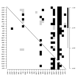
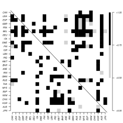
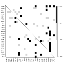
Notes: Posterior inclusion probabilities of spatial links based on MCMC draws. Inclusion probabilities 0.50-0.75 (little evidence for inclusion) are coloured grey. Strong evidence for inclusion (>0.75) indicated by black colour. Level specifications refer to specifications by using (all else being equal) log levels of infection rates rather than log-differences as the dependent variable.
[tbp] Fixed Sparsity Fixed Sparsity Mean Std.Dev. Mean Std.Dev. Mean Std.Dev. Mean Std.Dev. Initial infections -0.9538 0.0108 -0.9715 0.0093 -0.9718 0.0217 -0.9655 0.0223 Stringency -0.4062 0.0472 -0.5259 0.0360 -0.4856 0.0739 -0.3712 0.0738 Precipitation 0.0084 0.0365 -0.0304 0.0357 -0.0966 0.1023 -0.1284 0.1071 Temperature -0.0025 0.0017 -0.0018 0.0017 -0.0116 0.0047 -0.0172 0.0048 0.0801 0.0018 0.0960 0.0026 0.3624 0.0452 0.2526 0.0484 0.0264 0.0018 0.0266 0.0018 0.2318 0.0151 0.2457 0.0164 Avg. # neighbours 10.8863 6.5014 2.5103 2.0225 Fixed effects Yes Yes Yes Yes 27 27 27 27 19 19 19 19
-
•
Notes: Posterior quantities based on MCMC draws, where the first were discarded as burn-ins. Values in bold denote significance under a 90% credible interval.
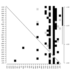
Notes: Posterior inclusion probabilities of spatial links based on MCMC draws. Inclusion probabilities 0.50-0.75 (little evidence for inclusion) are coloured grey. Strong evidence for inclusion (>0.75) indicated by black colour.
[tbp] Fixed Sparsity Fixed Sparsity Mean Std.Dev. Mean Std.Dev. Mean Std.Dev. Mean Std.Dev. Initial infections -0.9834 0.0161 -1.0090 0.0122 -1.0234 0.0207 -1.0016 0.0175 Stringency -0.2595 0.0853 -0.4966 0.0672 -0.1537 0.1667 0.0200 0.0822 Precipitation -0.0067 0.0453 0.0131 0.0440 -0.1114 0.0764 -0.1084 0.0724 Temperature 0.0030 0.0022 -0.0022 0.0024 -0.0093 0.0038 -0.0062 0.0037 0.7148 0.0111 0.4405 0.0164 0.8910 0.0317 0.8930 0.0359 0.0183 0.0019 0.0193 0.0019 0.0570 0.0060 0.0513 0.0064 Avg. # neighbours 10.4409 3.5630 3.1953 2.4116 Fixed effects Yes Yes Yes Yes 27 27 27 27 10 10 10 10
-
•
Notes: Posterior quantities based on MCMC draws, where the first were discarded as burn-ins. Values in bold denote significance under a 90% credible interval.
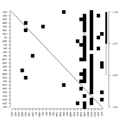
Notes: Posterior inclusion probabilities of spatial links based on MCMC draws. Inclusion probabilities 0.50-0.75 (little evidence for inclusion) are coloured grey. Strong evidence for inclusion (>0.75) indicated by black colour.
Notes: Trace plots and posterior densities based on MCMC draws, where the first were discarded as burn-ins. Dashed lines denote prior distributions.