D-STEM v2: A Software for Modelling Functional Spatio-Temporal Data

Yaqiong Wang, Francesco Finazzi, and Alessandro Fassò Modelling functional spatio-temporal data with D-STEM Modelling functional spatio-temporal data with D-STEM Functional spatio-temporal data naturally arise in many environmental and climate applications where data are collected in a three-dimensional space over time. The MATLAB D-STEM v1 software package was first introduced for modelling multivariate space-time data and has been recently extended to D-STEM v2 to handle functional data indexed across space and over time. This paper introduces the new modelling capabilities of D-STEM v2 as well as the complexity reduction techniques required when dealing with large data sets. Model estimation, validation and dynamic kriging are demonstrated in two case studies, one related to ground-level air quality data in Beijing, China, and the other one related to atmospheric profile data collected globally through radio sounding. functional data analysis, 4D data, climate data, environmetrics, EM algorithm functional data analysis, 4D data, climate data, environmetrics, EM algorithm Yaqiong Wang
Guanghua School of Management
Peking University
Yiheyuan road, 5
100871 Peking, China
E-mail:
Francesco Finazzi
Department of Management, Information and Production Engineering
University of Bergamo
viale Marconi, 5
24044 Dalmine (BG), Italy
E-mail:
URL: http://www.unibg.it/pers/?francesco.finazzi
Alessandro Fassò
Department of Management, Information and Production Engineering
University of Bergamo
viale Marconi, 5
24044 Dalmine (BG), Italy
E-mail:
URL: http://www.unibg.it/pers/?alessandro.fasso

1 Introduction

With the increase of multidimensional data availability and modern computing power, statistical models for spatial and spatio-temporal data are developing at a rapid pace. Hence, there is a need for stable and reliable, yet updated and efficient, software packages. In this section, we briefly discuss multidimensional data in climate and environmental studies as well as statistical software for space-time data.

1.1 Multidimensional data

Large multidimensional data sets often arise when climate and environmental phenomena are observed at the global scale over extended periods. In climate studies, relevant physical variables are observed on a three-dimensional (3D) spherical shell (the atmosphere) while time is the fourth dimension. For instance, measurements are obtained by radiosondes flying from ground level up to the stratosphere (fasso2014statistical), by interferometric sensors aboard satellites (finazzi2018statistical) or by laser-based methods, such as Light Detection and Ranging (LIDAR) (negri2018modeling). In this context, statistical modelling of multidimensional data requires describing and exploiting the spatio-temporal correlation of the underlying phenomenon or data-generating process. This is done using explanatory variables and multidimensional latent variables with covariance functions defined over a convenient spatio-temporal support. When considering 3D$\times$T data (4D for brevity), covariance functions defined over the 4D support may be adopted. However, these covariance functions often have a complex form (Porcu2018). Moreover, when estimating the model parameters or making inferences, very large covariance matrices (though they may be sparse) are implied.
In large climate and environmental applications, 4D data are rarely collected at high frequency in all spatial and temporal dimensions. Often, only one dimension is sampled at high frequency while the remaining dimensions are sampled sparsely. Radiosonde data, for instance, are sparse over the Earth’s sphere, but they are dense along the vertical dimension, providing atmospheric profiles. This suggests that handling all spatial dimensions equally (e.g. using a 3D covariance function) may not be the best option from a modelling or computational perspective, and a data reduction technique may be useful instead. In this paper, the functional data analysis (FDA) approach (ramsay2007applied) is adopted to model the relationship between measurements along the profile, while the remaining dimensions are handled following the classic spatio-temporal data modelling approach using only 2D spatial covariance functions.

1.2 Statistical software

Various software programmes are available for considering data on a plane or in a two-dimensional (2D) Euclidean space. The choice is more restricted when considering multidimensional or non-Euclidean spaces arising from atmospheric or remote sensing spatio-temporal data observed on the surface of a sphere and over time.

For example, Figure 1 depicts the spatial locations of measurements collected globally in a single day through radio sounding, as discussed in Section LABEL:sec:casestudy_climate. Space is three-dimensional, and measurements are repeated over time at the same spatial locations over the Earth’s surface but at different pressure values.

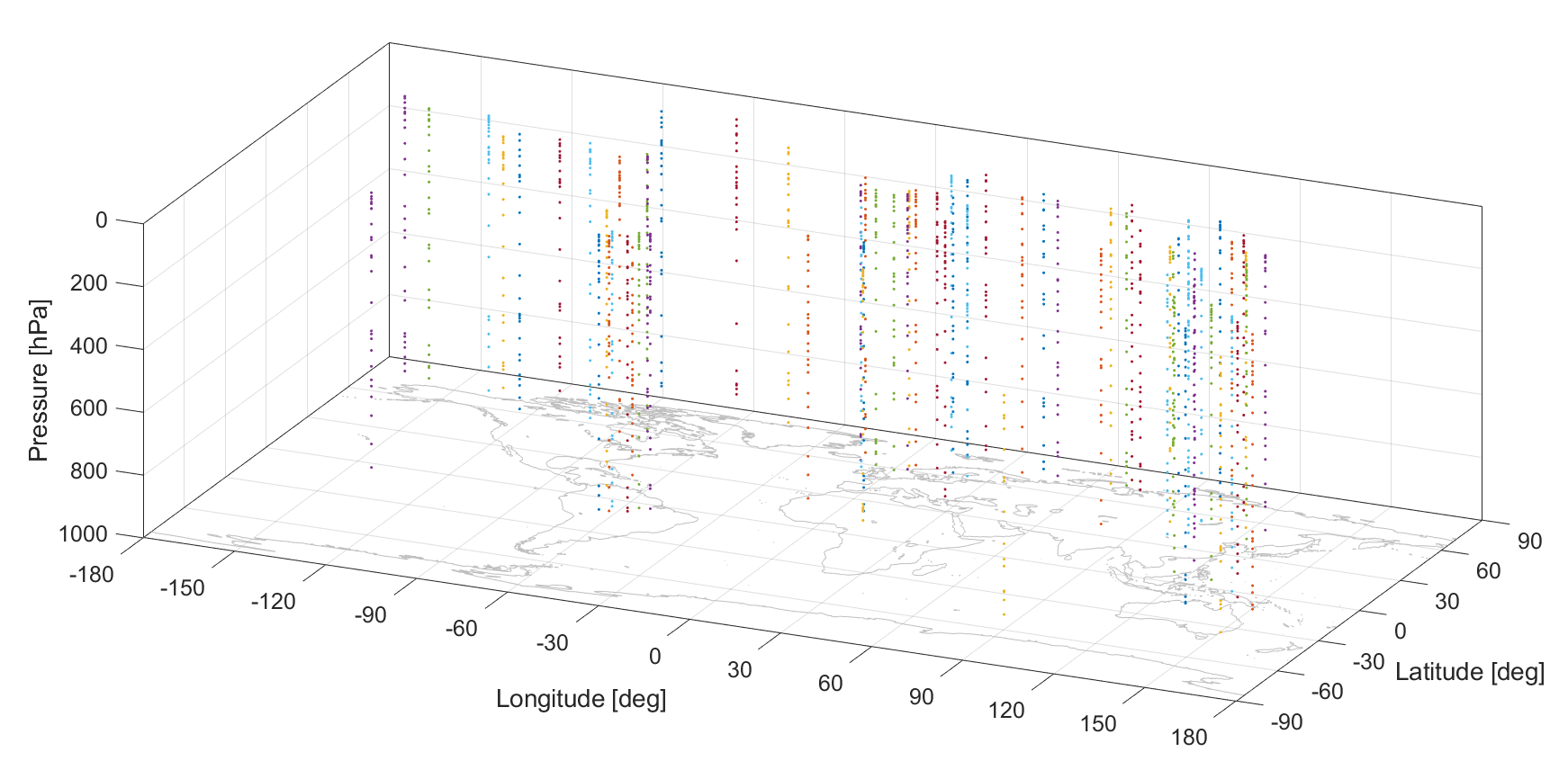
Figure 1: Radio sounding data example. Each dot represents the spatial location of a measurement taken by a radiosonde. Dots of the same colour belong to the same radiosonde. (Pressure axis not in scale).

The spBayes package (finley2015) handles large spatio-temporal data sets, but space is only 2D. The documentation of the spacetime (pebesma2012) and gstat (pebesma2016) packages does not explicitly address the multidimensional case, but, according to gasch2015, both packages have some capabilities to handle the 3D$\times$T. However, we want to avoid working with 3D spatial covariance functions or sample spatio-temporal variograms. Fixed rank kriging (cressie2008fixed cressie2008fixed) implemented in the R package FRK (zammit2018frk) handles spatial and spatio-temporal data both on the Euclidean plane and on the surface of the sphere. FRK implements a set of tools for data gridding and basis function computation, resulting in efficient dimension reduction, allowing it to handle large satellite data sets (cressie2018mission). It is based on a spatio-temporal random effects (SRE) model estimated by the expectation-maximisation (EM) algorithm. Recent extensions to FRK include the use of multi-resolution basis functions (tzeng2018resolution).

A second package based on SRE and the EM algorithm is D-STEM v1 (finazzi2014d). This package implements an efficient state-space approach for handling the temporal dimension and a heterotopic multivariate response approach that is useful when correlating heterogeneous networks (fasso2011; calculli2015maximum).

D-STEM v1 has been successfully used in various medium-to-large applications, proving that the EM algorithm implementation, being mainly based on closed-form iterations, is quite stable. These applications include air quality assessment in the metropolitan areas of Milan, Teheran and Beijing (fasso2013; Taghavi2019; Wan2020ENV); multivariate spatio-temporal modelling at the country and continental levels in Europe (finazzi2013; fasso2016); time series clustering (finazzi2015); emulators of atmospheric dispersion modelling systems (finazzi2019); and near real-time prediction of earthquake parameters (finazzi2020).

A brief, non-exhaustive list of other models and/or software packages for advanced spatial data modelling is presented below, according to the principal technique, allowing the handling of large data sets. In general, these techniques aim at avoiding the Cholesky decomposition of large and dense covariance matrices.

Some approaches, including FRK and D-STEM v1, leverage sparse variance–covariance matrices. Others exploit the sparsity of the precision matrix, thanks to a spatial Markovian assumption. This class includes the R packages LatticeKrig (nychka2015multiresolution; Nychka2016), INLA (blangiardo2013; lindgren2015; Bivand2015; rue2014) and the multi-resolution approximation approach of katzfuss2017multi, which uses the predictive process and the state space representation (jurek2018multi) to model spatio-temporal data. Low-rank models are another popular approach used by spBayes. Finally, the R package laGP (gramacy2016lagp), based on a machine learning approach, implements an efficient nearest neighbour prediction-oriented method. heaton2018case develop an interesting spatial prediction competition considering a large data set and involving the above-mentioned approaches.

We observe that, although some of the software packages mentioned above consider both space and time, to the best of our knowledge, none of them handles a spatio-temporal FDA approach for data sets of the kind discussed in 1.1.

In this paper, we present D-STEM v2, which is a MATLAB package, extending D-STEM v1. The new version introduces modelling of functional data indexed over space and time. Moreover, new complexity reduction techniques have been added for both model estimation and dynamic mapping, which are especially useful for large data sets.
The rest of the paper is organised as follows. Section 2 introduces the methodology adopted in this paper and, in particular, the data modelling approach and the complexity-reduction techniques. Section 3 describes the D-STEM v2 software in terms of the MATLAB classes used to define the data structure, model fitting and diagnostics and kriging. This is followed by an illustration of the software use through two case studies. The first one, discussed in Section 4, considers high-frequency spatio-temporal ozone data in Beijing. The second one, in Section LABEL:sec:casestudy_climate, considers modelling of global atmospheric temperature profiles and exploits the complexity-reduction capabilities of the new package. Finally, concluding remarks are provided in Section LABEL:sec:remarks.

2 Methodology

This section discusses the methodology behind the modelling and the complexity-reduction techniques implemented in D-STEM v2 when dealing with functional space-time data sets. Moreover, model estimation, validation and dynamic kriging are briefly discussed.

2.1 Model equations

Let $\bm{s}=(s_{lat},s_{lon})^{\top}$ be a generic spatial location on the Earth’s sphere, $\mathbb{S}^{2}$, and $t\in\mathbb{N}$ a discrete time index. It is assumed that the function of interest, $f\left(\bm{s},h,t\right)$, with domain $\mathcal{H}=\left[h_{1},h_{2}\right]\subset\mathbb{R}$, can be observed at any $\left(\bm{s},t\right)$ and $h\in\mathcal{H}$ through noisy measurements $y(\bm{s},h,t)$ according to the following model:

$$y(\bm{s},h,t) =f\left(\bm{s},h,t\right)+\varepsilon(\bm{s},h,t),$$ (1)

$$f\left(\bm{s},h,t\right) =\bm{x}(\bm{s},h,t)^{\top}\bm{\beta}\left(h\right)+\bm{\phi}(h)^{\top}\bm{z}(\bm{s},t),$$ (2)

$$\bm{z}(\bm{s},t) =\bm{G}\bm{z}(\bm{s},t-1)+\bm{\eta}(\bm{s},t).$$ (3)

This model is referred to as the functional hidden dynamic geostatistical model (f-HDGM). In Equation (1), $\varepsilon$ is a zero-mean Gaussian measurement error independent in space and time with functional variance $\sigma_{\varepsilon}^{2}\left(h\right)$, implying that $\varepsilon$ is heteroskedastic across the domain $\mathcal{H}$. The variance is modelled as

$$\log(\sigma_{\varepsilon}^{2}\left(h\right))=\bm{\phi}(h)^{\top}\bm{c}_{\varepsilon},$$

where $\bm{\phi}(h)$ is a $p\times 1$ vector of basis functions evaluated at $h$, while $\bm{c}_{\varepsilon}$ is a vector of coefficients to be estimated. In Equation (2), $\bm{x}(\bm{s},h,t)$ is a $b\times 1$ vector of covariates while $\bm{\beta}\left(h\right)=(\beta_{1}(h),...,\beta_{b}(h))^{\top}$ is the vector of functional parameters modelled as

$$\beta_{j}(h)=\bm{\phi}(h)^{\top}\bm{c}_{\beta,j},j=1,...,b,$$

and $\bm{c}_{\beta}=\left(\bm{c}_{\beta,1}^{\top},...,\bm{c}_{\beta,b}^{\top}\right)^{\top}$ is a $pb\times 1$ vector of coefficients that needs to be estimated. Additionally, $\bm{z}(\bm{s},t)$ is a $p\times 1$ latent space-time variable with Markovian dynamics given in Equation (3). The matrix $\bm{G}$ is a diagonal transition matrix with diagonal elements in the $p\times 1$ vector $\bm{g}$. The innovation vector $\bm{\eta}$ is obtained from a multivariate Gaussian process that is independent in time but correlated across space with matrix spatial covariance function given by

$$\bm{\Gamma}(\bm{s},\bm{s}^{\prime};\bm{\theta})=diag\left(v_{1}\rho(\bm{s},\bm{s}^{\prime};\bm{\theta}_{1}),...,v_{p}\rho(\bm{s},\bm{s}^{\prime};\bm{\theta}_{p})\right),$$

where $\bm{v}=\left(v_{1},...,v_{p}\right)^{\top}$ is a vector of variances and $\rho(\bm{s},\bm{s}^{\prime};\bm{\theta}_{j})$ is a valid spatial correlation function for locations $\bm{s},\bm{s}^{\prime}\in\mathbb{S}^{2}$, parametrised by $\bm{\theta}_{j}$, and $\bm{\theta}=(\bm{\theta}_{1},...,\bm{\theta}_{p})^{\top}$. The unknown model parameter vector is given by $\bm{\psi}=\left(\bm{c}_{\varepsilon}^{\top},\bm{c}_{\beta}^{\top},\bm{g}^{\top},\bm{v}^{\top},\bm{\theta}^{\top}\right)^{\top}$.

Note that, in order to ease the notation, the same $p$-dimensional basis functions $\bm{\phi}(h)$ are used to model $\sigma_{\varepsilon}^{2}$, $\beta_{j}$ and $\bm{\phi}(h)^{\top}\bm{z}(\bm{s},t)$ in Equations (1)-(3). In practice, D-STEM v2 allows one to specify a different number of basis functions for each model component. Also note that $\varepsilon$ is not a pure measurement error since it also accounts for model misspecification. Finally, the covariates $\bm{x}(\bm{s},h,t)$ are assumed to be known without error for any $\bm{s}$, $h$ and $t$, and thus they do not need a basis function representation.

2.2 Basis function choice

Choosing basis functions essentially means choosing the basis type and the number of basis functions. D-STEM v2 currently supports Fourier bases and B-spline bases. The former guarantee that the function is periodic in the domain $\mathcal{H}$, while the latter are not (in general) periodic but have higher flexibility in describing functions with a complex shape. Whichever basis function type is adopted, the number $p$ of basis functions must be fixed before model estimation. Usually, a high $p$ implies a better model $R^{2}$, but over-fitting may be an issue. Moreover, special care must be taken when choosing the number of basis functions for $\bm{\phi}(h)^{\top}\bm{z}(\bm{s},t)$. The classic FDA approach suggests fixing a high number of basis functions and adopting penalisation to avoid over-fitting. In our context, this is not viable since the covariance matrices involved in model estimation have dimension $n^{3}p^{3}\times n^{3}p^{3}$. Since $n$ is usually large, a large $p$ would make model estimation unfeasible, especially if the number of time points $T$ is also high. When using B-spline basis, a small $p$ implies that the location of knots along the domain $\mathcal{H}$ also matters and may affect the model fitting performance. Ideally, $p$ and knot locations are chosen using a model validation technique (see 2.7) by trying different combinations of $p$ and knot locations. If, due to time constraints, this is not possible, equally spaced knots are a convenient option.

2.3 Model estimation

The estimation of $\bm{\psi}$ and the latent space-time variable $\bm{z}(\bm{s},t)$ is based on the maximum likelihood approach considering profile data observed at spatial locations $\mathcal{S}=\{\bm{s}_{i},i=1,...,n\}$ and time points $t=1,...,T$.

At a specific location $\bm{s}_{i}$ and time $t$, $q_{i,t}$ measurements are taken at points $\bm{h}_{\bm{s}_{i},t}=\left(h_{i,1,t},...,h_{i,q_{i,t},t}\right)^{\top}$ and collected in the vector

$$\bm{y}_{\bm{s}_{i},t}=(y(\bm{s}_{i},h_{i,1,t},t),...,y(\bm{s}_{i},h_{i,q_{i,t},t},t))^{\top},$$

here called the observed profile.

Although D-STEM v2 allows for varying $q_{i,t}$, for ease of notation, it is assumed here that all profiles include exactly $q$ measurements, although $\bm{h}_{\bm{s}_{i},t}$ may be different across profiles. Profiles observed at time $t$ across spatial locations $\mathcal{S}$ are then stored in the $nq\times 1$ vector $\bm{y}_{t}=(\bm{y}_{s_{1},t}^{\top},...,\bm{y}_{s_{n},t}^{\top})^{\top}$. Applying model (1)-(3) to the defined data above, we have the following matrix representation:

$$\bm{y}_{t} =\tilde{\bm{X}}_{t}\bm{c}_{\bm{\beta}}+\bm{\Phi}_{\bm{z},t}\bm{z}_{t}+\bm{\varepsilon}_{t},$$

$$\bm{z}_{t} =\tilde{\bm{G}}\bm{z}_{t-1}+\bm{\eta}_{t},$$

where $\tilde{\bm{X}}_{t}=\bm{X}_{t}\bm{\Phi}_{\bm{\beta},t}$ is a $nq\times bp$ matrix, with $\bm{X}_{t}$ the matrix of covariates and $\bm{\Phi}_{\bm{\beta},t}$ the basis matrix for $\bm{\beta}$. $\bm{\Phi}_{\bm{z},t}$ is the $nq\times np$ basis matrix for the latent $np\times 1$ vector $\bm{z}_{t}=(\bm{z}(\bm{s}_{1},t)^{\top},...,\bm{z}(\bm{s}_{n},t)^{\top})^{\top}$. $\bm{\eta}_{t}=(\bm{\eta}(\bm{s}_{1},t)^{\top},...,\bm{\eta}(\bm{s}_{n},t)^{\top})^{\top}$ is the $np\times 1$ innovation vector, while $\bm{\varepsilon}_{t}\$ is the $nq\times 1$ vector of measurement errors. Additionally, $\tilde{\bm{G}}=\bm{I}_{n}\otimes\bm{G}$ is the $np\times np$ diagonal transition matrix.

The complete-data likelihood function $L(\bm{\psi};\bm{Y},\bm{Z})$ can be written as

$$L(\bm{\psi};\bm{Y},\bm{Z})=L(\bm{\psi}_{\bm{z}_{0}};\bm{z}_{0})\prod_{t=1}^{T}L(\bm{\psi}_{\bm{y}};\bm{y}_{t}|\bm{z}_{t})L(\bm{\psi}_{\bm{z}};\bm{z}_{t}|\bm{z}_{t-1}),$$

where $\bm{Y}=\left(\bm{y}_{1},...,\bm{y}_{T}\right)$, $\bm{Z}=\left(\bm{z}_{0},\bm{z}_{1},...,\bm{z}_{T}\right)$, $\bm{\psi}_{\bm{z}}=\left(\bm{g}^{\top},\bm{v}^{\top},\bm{\theta}^{\top}\right)^{\top}$, $\bm{\psi}_{\bm{y}}=\left(\bm{c}_{\varepsilon}^{\top},\bm{c}_{\beta}^{\top}\right)^{\top}$, and $\bm{z}_{0}$ is the Gaussian initial vector with parameter $\bm{\psi}_{\bm{z}_{0}}$. Maximum likelihood estimation is based on an extension of the EM algorithm detailed in calculli2015maximum. The model parameter set $\bm{\psi}$ is initialised with starting values $\bm{\psi}^{\left\langle 0\right\rangle}$ and then updated at each iteration $\iota$ of the EM algorithm.

The algorithm terminates if any of the following conditions is satisfied:

$$\max_{l}\left|\psi_{l}^{\left\langle\iota\right\rangle}-\psi_{l}^{\left\langle\iota-1\right\rangle}\right|/\left|\psi_{l}^{\left\langle\iota\right\rangle}\right|<\epsilon_{1}$$

$$\left|L(\bm{\psi}^{\left\langle\iota\right\rangle};\bm{Y})-L(\bm{\psi}^{\left\langle\iota-1\right\rangle};\bm{Y})\right|/\left|L(\bm{\psi}^{\left\langle\iota\right\rangle};\bm{Y})\right|<\epsilon_{2},$$

$$\iota>\iota^{\ast},$$

where $\psi_{l}^{\left\langle\iota\right\rangle}$ is the generic element of $\bm{\psi}^{\left\langle\iota\right\rangle}$ at the $\iota\text{-}th$ iteration, $L(\bm{\psi}^{\left\langle\iota\right\rangle};\bm{Y})$ is the observed-data likelihood function evaluated at $\bm{\psi}^{\left\langle\iota\right\rangle}$, $0<\epsilon_{1}\ll 1$ and $0<\epsilon_{2}\ll 1$ are small positive numbers

(e.g. $10^{-4}$), while $\iota^{\ast}$ is a user-defined positive integer number (e.g. $100$) to limit the iterations in the case of convergence failure of the EM algorithm.

Note that $\mathcal{S}$ is not time-varying, which means that spatial locations are fixed. This could be a limit in applications where spatial locations change for each $t$. On the other hand, missing profiles are allowed; that is, $\bm{y}_{\bm{s}_{i},t}$ may be a vector of $q$ missing values at some $t$. In the extreme case, a given spatial location $\bm{s}_{i}$ has only one profile over the entire period (if all the profiles are missing, the spatial location can be dropped from the data set). shumway2017 explains how the likelihood function of a state-space model changes in the case of a missing observation vector and how the EM estimation formulas are derived. Missing data handling in D-STEM v2 is based on the same approach.

2.4 Partitioning

At each iteration of the EM algorithm, the computational complexity of the E-step is $O\left(Tn^{3}p^{3}\right)$, which may be unfeasible if $n$ is large. When necessary, D-STEM v2 allows one to use a partitioning approach (stein2013) for model estimation. The spatial locations $\mathcal{S}$ are divided into $k$ partitions, and $\bm{z}_{t}$ is partitioned conformably, namely, $\bm{z}_{t}=\left(\bm{z}_{t}^{(1)\top},...,\bm{z}_{t}^{(k)\top}\right)^{\top}$. Hence, the likelihood function becomes

$${\prod\limits_{t=1}^{T}}L\left(\bm{\psi}_{\bm{y}};\bm{y}_{t}\mid\bm{z}_{t}\right)\cdot{\prod\limits_{j=1}^{k}}L\left(\bm{\psi}_{\bm{z}_{0}};\bm{z}_{0}^{(j)}\right)\cdot{\prod\limits_{j=1}^{k}}{\prod\limits_{t=1}^{T}}L\left(\bm{\psi}_{\bm{z}};\bm{z}_{t}^{(j)}\mid\bm{z}_{t-1}^{(j)}\right).$$

From the EM algorithm point of view, this implies that the E-step is independently applied to each partition, possibly in parallel. When all partitions are equal in size, the computational complexity reduces to $\mathcal{O}\left(Tkr^{3}p^{3}\right)$, with $r$ as the partition size.

Geographical partitioning, constructed aggregating proximal locations, is a natural choice for environmental applications. Given the number of partitions $k$, the k-means algorithm applied to spatial coordinates provides a geographical partitioning of $\mathcal{S}$. However, the number of points in each partition is not controlled, and a heterogeneous partitioning may arise. If some subsets are very large and others are small, the reduction in computational complexity given above is far from being achieved. This can easily happen, for example, when $\mathcal{S}$ is a global network constrained by continent shapes.

For this reason, D-STEM v2 provides a heuristically modified k-means algorithm that encourages partitions with similar numbers of elements. The algorithm optimises the following objective function:

$$\sum_{j=1}^{k}\sum_{\bm{s}\in\mathcal{S}_{j}}d\left(\bm{s},\bm{c}_{j}\right)+\lambda\sum_{j=1}^{k}\left(r_{j}-\frac{n}{k}\right)^{2},$$ (4)

where $\lambda\geq 0$, $\mathcal{S}_{j}\subset\mathcal{S}$ is the set of coordinates in the $j\text{-}th$ partition, $d$ is the geodesic distance on the sphere $\mathbb{S}^{2}$ and $\bm{c}_{j}$ and $r_{j}$ are the centroid and the number of elements in the $j\text{-}th$ partition, respectively.
The second term in (4) accounts for the variability of the partition sizes and acts as a penalisation for heterogeneous partitionings. Clearly, when $\lambda=0$, the above-mentioned objective function gives the classic k-means algorithm. For high values of $\lambda$, solutions with similarly sized partitions are favoured.
Unfortunately, an optimality theory for this algorithm has not yet been developed, and the choice of $\lambda$ is left to the user. Nonetheless, it may be a useful tool to define a partitioning that is appropriate for the application at hand with regard to computing time and geographical properties.

2.5 Variance-covariance matrix estimation

The EM algorithm provides a point estimate of the parameter vector $\bm{\psi}$ but no uncertainty information. Building on shumway2017, D-STEM v2 estimates the variance–covariance matrix $\Sigma_{\bm{\psi},T}=\mathbb{V}\left(\bm{\psi}\mid\bm{Y}\right)$, by means of the observed Fisher information matrix, $\mathbf{I}_{T}$, namely

$$\hat{\Sigma}_{\bm{\psi},T}=(\mathbf{I}_{T})^{-1}.$$

To understand its computational cost, note that the information matrix given above may be written as a sum: $\mathbf{I}_{T}=\sum_{t=1}^{T}\mathbf{i}_{t}$.
For large data sets, each matrix $\mathbf{i}_{t}$ may be expensive to compute, and the total computational cost is linear in $T$, provided missing data are evenly distributed in time. This results in a time-consuming task with a computational burden even higher than that for model estimation. For this reason, D-STEM v2 makes it possible to approximate $\hat{\Sigma}_{\bm{\psi},T}$ using a truncated information matrix, namely:

$$\tilde{\Sigma}_{\bm{\psi},t^{*}}=(\frac{T}{t^{*}}\mathbf{I}_{t^{*}})^{-1},$$ (5)

which reduces the computational burden by a factor of $1-t^{*}/T$.
Since $\tilde{\Sigma}_{\bm{\psi},t^{*}}\rightarrow\hat{\Sigma}_{\bm{\psi},T}$ for $t^{*}\rightarrow T$, the truncation time $t^{*}$ is chosen to control the approximation error in $\hat{\Sigma}_{\bm{\psi}}$. In particular, $t^{*}$ is the first integer such that

$$\frac{\left\|\tilde{\Sigma}_{\bm{\psi},t}-\tilde{\Sigma}_{\bm{\psi},t-1}\right\|_{F}}{\left\|\tilde{\Sigma}_{\bm{\psi},t}\right\|_{F}}\leq\delta,$$ (6)

where $\left\|{\cdot}\right\|_{F}$ is the Frobenius norm, and $\delta$ may be defined by the user.
Generally speaking, the behaviour of $\hat{\Sigma}_{\bm{\psi},T}$ for large $T$ and, hence, the behaviour of $\tilde{\Sigma}_{\bm{\psi},t}$ relays on stationarity and ergodicity of the underlying stochastic process; see, for example, shumway2017 and references therein.
To have operative guidance for the user, let us assume first that no missing values are present, the information matrix is well-conditioned and the covariates have no isolated outliers or extreme trends. In this case, away from the borders $t\cong 1$ and $t\cong T$, the observed conditional information $\mathbf{i}_{t}$ has a relatively smooth stochastic behaviour, and the approximation in (5) is expected to be satisfactory at the level defined by $\delta$. Conversely, if some data are missing at time $t$, the information $\mathbf{i}_{t}$ is reduced accordingly. If the missing pattern is random over time, this is not an issue. But, in the unfavourable case with a high percentage of missing data mostly concentrated at the end the time series, $t\cong T$, the above approximation may over-estimate the information and under-estimate the variances of the parameter estimates.

2.6 Dynamic kriging

In this paper, dynamic kriging refers to evaluating the following quantities:

$$\hat{f}\left(\bm{s},h,t\right) =\mathbb{E}_{\hat{\bm{\psi}}}\left(f\left(\bm{s},h,t\right)\mid\bm{Y}\right),$$ (7)

$$\VAR\left(\hat{f}\left(\bm{s},h,t\right)\right) =\mathbb{V}_{\hat{\bm{\psi}}}\left(f\left(\bm{s},h,t\right)\mid\bm{Y}\right),$$ (8)

for any $\bm{s}\in\mathbb{S}^{2}$, $h\in\mathcal{H}$ and $t=1,...,T$. A common approach is to map the kriging estimates on a regular pixelation $\mathcal{S}^{\ast}=\left\{\bm{s}_{1}^{\ast},...,\bm{s}_{m}^{\ast}\right\}$. This may be a time-consuming task when $m$ and/or $n$ and/or $T$ are large. To tackle this problem, D-STEM v2 allows one to exploit a nearest-neighbour approach, where the conditioning term in Equations (7) and (8) is not $\bm{Y}$, but the data at the spatial locations $\mathcal{S}_{\sim j}$, where $\mathcal{S}_{\sim j}\subset\mathcal{S}$ is the set of the $\tilde{n}\ll n$ nearest spatial locations to $\bm{s}_{j}^{\ast}$. The use of the nearest-neighbour approach is justified by the so-called screening effect. Even when the spatial correlation function exhibits long-range dependence, it can subsequently be assumed that $y$ at spatial location $\bm{s}$ is nearly independent of spatially distant observations when conditioned on nearby observations (see Stein2002; furrer2006, for more details).

For computational efficiency, D-STEM v2 performs kriging for blocks of pixels. To do this, $\mathcal{S}^{\ast}$ is partitioned in $u$ blocks $\mathcal{S}^{\ast}=\left\{\mathcal{S}_{1}^{\ast},...,\mathcal{S}_{u}^{\ast}\right\}$, and kriging is done on each block $\mathcal{S}_{l}^{\ast}$, $l=1,...,u$, with $u\ll m$ controlled by the user. For each target block $\mathcal{S}_{l}^{\ast}$, the conditioning term in Equations (7) and (8) is given by the data observed at $\mathcal{\tilde{S}}_{l}=\bigcup\nolimits_{j\in\mathcal{J}_{l}}\mathcal{S}_{\sim j},\mathcal{J}_{l}=\left\{j:s_{j}^{\ast}\in\mathcal{S}_{l}^{\ast}\right\}$. Note that, if $\mathcal{S}_{l}^{\ast}$ is dense and $\mathcal{S}$ is sparse (namely $n\ll m$), then $\mathcal{\tilde{S}}_{l}$ is not much larger than $\mathcal{S}_{\sim j}$ since most of the spatial locations in $\mathcal{S}_{l}^{\ast}$ tend to have the same neighbours $\mathcal{S}_{\sim j}$.

2.7 Validation

D-STEM v2 allows one to implement an out-of-sample validation by partitioning the original spatial locations $\mathcal{S}$ into subsets $\mathcal{S}_{est}$ and $\mathcal{S}_{val}$. Data at $\mathcal{S}_{est}$ are used for model estimation while data at $\mathcal{S}_{val}$ are used for validation. Once the model is estimated, the kriging formula in Equation (7) is used to predict at $\mathcal{S}_{val}$ for all times $t$ and heights $\bm{h}$. The following validation mean squared errors are then computed

$$MSE_{t} =\frac{1}{P_{1}}\sum_{\bm{s}\in\mathcal{S}_{val}}\sum_{h\in\bm{h}_{\bm{s},t}}\left(y\left(\bm{s},h,t\right)-\hat{y}\left(\bm{s},h,t\right)\right)^{2},$$

$$MSE_{\bm{s}} =\frac{1}{P_{2}}\sum_{t=1}^{T}\sum_{h\in\bm{h}_{\bm{s},t}}\left(y\left(\bm{s},h,t\right)-\hat{y}\left(\bm{s},h,t\right)\right)^{2},$$

$$MSE_{h} =\frac{1}{P_{3}}\sum_{t=1}^{T}\sum_{\bm{s}\in\mathcal{S}_{val}}\left(y\left(\bm{s},h,t\right)-\hat{y}\left(\bm{s},h,t\right)\right)^{2},$$

where $\hat{y}\left(\bm{s},h,t\right)$ is obtained from Equation (7), while $P_{1}$, $P_{2}$ and $P_{3}$ are the number of terms in each sum.

When $\bm{h}_{\bm{s},t}$ varies across the profiles, D-STEM v2 provides a binned MSE by splitting the continuous domain $\mathcal{H}$ into $B$ equally spaced intervals. Let $H^{*}_{r}$ be the set of observation points in the $r\text{-}th$ interval, let $n_{r}$ be the corresponding observation number and let $\bar{h}_{r}=\frac{1}{n_{r}}\sum_{h\in H^{*}_{r}}h$ be the mean of points in $b\text{-}th$ interval. Then, the $MSE_{\bar{h}_{r}}$ is computed by

$$MSE_{\bar{h}_{r}} =\frac{1}{P_{4}}\sum_{h\in H^{*}_{r}}\sum_{t=1}^{T}\sum_{\bm{s}\in\mathcal{S}_{val}}\left(y\left(\bm{s},h,t\right)-\hat{y}\left(\bm{s},h,t\right)\right)^{2},$$

where $P_{4}$ is the total number of observations in the $b\text{-}th$ interval.

D-STEM v2 also provides the validation $R^{2}$ with respect to time

$$R^{2}_{t} =1-\frac{MSE_{t}}{\VAR\left(\{y\left(\bm{s},h,t\right),\bm{s}\in\mathcal{S}_{val},h\in\bm{h}_{\bm{s},t}\}\right)}.$$

and the analogous validation $R^{2}$ with respect to location $\bm{s}$ and $h_{r}$.

3 Software

This section starts by briefly describing the modelling capabilities of D-STEM v2 inherited by the previous version for dealing with spatio-temporal data sets. Then, it focuses on the D-STEM v2 classes and methods, which implement estimation, validation and dynamic mapping of the model presented in Section 2. Although some of the classes are already available in D-STEM v1, they are listed here for completeness.

3.1 Software description

D-STEM v1 implemented a substantial number of models. The dynamic coregionalisation model (DCM, finazzi2014d finazzi2014d) and the hidden dynamic geostatistical model (HDGM, calculli2015maximum calculli2015maximum) are suitable for modelling and mapping multivariate space-time data collected from unbalanced monitoring networks. Model-based clustering (MBC, finazzi2015 finazzi2015) has been introduced for clustering time series, and it is suitable for large data sets with spatially registered time series. Moreover, the emulator model (finazzi2019) is based on a Gaussian emulator, and it is exploited for modelling the multivariate output of a complex physical model.

In addition, D-STEM v2 (available at github.com/graspa-group/d-stem) provides the functional version of HDGM, denoted by f-HDGM, which handles modelling and mapping of functional space-time data, following the methodology of Section 2. For implementing f-HDGM, D-STEM v2 relies on the MATLAB version of the fda package (ramsay2018), which is automatically downloaded and installed by D-STEM v2.

3.2 Data format

Two data formats are available to define observations for the f-HDGM. One is the internal format used by the D-STEM v2 classes, and the other one is the user format based on the more user-friendly table data type implemented in recent versions of MATLAB. The latter permits storing measurement profiles, covariate profiles, coordinates, timestamps and units of measure in a single object. The internal format is not discussed here.
Considering a table in the user format, each row includes the profiles collected at a given spatial location and time point. The column labels are defined as follows: columns Y and Y_name are used for the dependent variable $y$ and its name as a string field, respectively; the column with prefix X_h_ is used for the values of the domain $h$; eventually, columns with prefix X_beta_ are used for covariates $\bm{x}$. These tables have only one column for $y$ and only one column for $h$. Instead, we can have any number $b\geqslant 0$ of covariate columns. Additionally, the table has columns X_coordinate and Y_coordinate for spatial location $\bm{s}$ and column Time for the timestamp. Units of measure are stored in the Properties.VariableUnits property of the table columns and used in outputs and plots. Units for X_coordinate and Y_coordinate can be deg for degrees, m for meters and km for kilometres. Geodetic distance is used when the unit is deg; otherwise, the Euclidean distance is used.
At the table row corresponding to location $\bm{s}_{i}$ and time $t$, the elements related to $y$ and $\bm{x}$ are vectors with $q_{i,t}$ elements. Vectors related to $y$ may include missing data (NaN). If $y$ is entirely missing for a given $\left(\bm{s},t\right)$, the row must be removed from the table. Since spatial locations $\mathcal{S}$ are fixed in time, and as their number $n$ is determined by the number of unique coordinates in the table, profiles observed at different time points but the same spatial location $\bm{s}$ must have the same coordinates.

3.3 Software structure

In D-STEM, a hierarchical structure of object classes and methods is used to handle data definition, model definition and estimation, validation, dynamic kriging and the related plotting capabilities. The structure is schematically given below. Further details on the use of each class are given within the two case studies in this paper, while class constructors, methods and property details can be obtained in MATLAB using the command

doc <class_name>.

3.3.1 Data handling

The stem_data class allows the user to define the data used in f-HDGM models, mainly through the following objects and methods.

• Objects of stem_data

  • stem_modeltype: model type (DCM, HDGM, MBC, Emulator or f-HDGM); note that model type is needed here because the data structure varies among the different models;

  • stem_fda: basis functions specification;

  • stem_validation (optional): definition of the learning and testing datasets for model validation.

• Methods and Properties of stem_data

  • kmeans_partitioning: data partitioning for parallel EM computations of Section 2.4; this method is applied to a stem_data object, and its output is used by the EM_estimation method in the stem_model class below;

  • shape (optional): structure with geographical borders used for mapping.

• Internal Objects of stem_data

  • stem_varset: observed data and covariates;

  • stem_gridlist: list of stem_grid objects

    • stem_grid: spatial locations coordinates;

  • stem_datestamp: temporal information.

Interestingly, stem_misc.data_formatter is a helper method, which is useful for building stem_varset objects starting from data tables. Its class, stem_misc, is a miscellanea static class implementing other methods for various intermediate tasks not discussed here for brevity.

3.3.2 Model building

The stem_model class is used to define, estimate, validate and output a f-HDGM, mainly through the following objects and methods.

• Objects of stem_model

  • stem_data: defined above;

  • stem_par: model parameters;

  • stem_EM_result: container of the estimation output, after EM_estimate;

  • stem_validation_result (optional): container of validation output, available only if stem_data contains the stem_validation object;

  • stem_EM_options (optional): model estimation options; it is an input of the EM_estimate method below.

• Methods of stem_model

  • EM_estimate: computation of parameter estimates;

  • set_varcov: computation of the estimated variance-covariance matrix;

  • plot_profile: plot of functional data;

  • print: print estimated model summary;

  • beta_Chi2_test: testing significance of covariates;

  • plot_par: plot functional parameter;

  • plot_validation: plot MSE validation.

3.3.3 Kriging

The kriging handling is implemented with two classes. The first is the stem_krig class, which implements the kriging spatial interpolation.

• Objects of stem_krig

  • stem_krig_data: mesh data for kriging;

  • stem_krig_options: kriging options;

• Methods of stem_krig

  • kriging: computation of kriging, the output is a stem_krig_result object.

The second is the stem_krig_result class, which stores the kriging output and implements the methods for plotting the kriging output.

• Methods of stem_krig_result

  • surface_plot: mapping of kriging estimate and their standard deviation for fixed $h$;

  • profile_plot: method for plotting the kriging function and the variance-covariance matrix for a fixed space and time.

Although at first reading the user could prefer a single object for both input and output of the kriging, these objects may be quite large, making the current approach more flexible.

4 Case study on ozone data

This section illustrates how to make inferences on an f-HDGM for ground-level high-frequency air quality data collected by a monitoring network. In particular, hourly ozone ($O_{3}$, in $\mu g/m^{3}$) measured in Beijing, China, is considered.

4.1 Air quality data

Ground-level $O_{3}$ is an increasing public concern due to its essential role in air pollution and climate change. In China, $O_{3}$ has become one of the most severe air pollutants in recent years (wang2017ozone).

In this case study, the aim is to model hourly $O_{3}$ concentrations from 2015 to 2017 with respect to temperature and ultraviolet radiation (UVB) across Beijing. Concentration and temperature data are available at twelve monitoring stations (Figure 2). Hourly UVB data are obtained from the ERA-Interim product of the European Centre for Medium-Range Weather Forecasts (ECMWF) at a grid size of $0.25^{\circ}\times 0.25^{\circ}$ over the city.

Figure 2: Spatial locations of the twelve stations in Beijing (david2013ggmap).

To describe the diurnal cycle of $O_{3}$, which peaks in the afternoon and reaches a minimum at night-time, the 24 hours of the day are used as domain $\mathcal{H}$ of the basis functions, while the time index $t$ is on the daily scale. Moreover, due to the circularity of time, Fourier basis functions are adopted, which implies that $\beta_{j}\left(h\right)$, $\sigma_{\varepsilon}^{2}\left(h\right)$ are periodic functions.

The measurement equation for $O_{3}$ is

$$y(\bm{s},h,t)=\beta_{0}(h)+x_{temp}(\bm{s},h,t)\beta_{temp}(h)+x_{uvb}\left(t\right)\beta_{uvb}(h)+\bm{\phi}(h)^{\top}\bm{z}(\bm{s},t)+\varepsilon(\bm{s},h,t),$$ (9)

where $\bm{s}$ is the generic spatial location, $h\in\left[0,24\right)$ is the time within the day expressed in hours and $t=1,...,1096$ is the day index over the period 2015–2017. Based on a preliminary analysis, the number of basis functions for $\beta_{j}\left(h\right)$, $\sigma_{\varepsilon}^{2}\left(h\right)$ and $\bm{\phi}(h)^{\top}\bm{z}(\bm{s},t)$ is chosen to be $5$, $5$ and $7$, respectively.

4.2 Software implementation

This paragraph details the implementation of the D-STEM v2 in three aspects: model estimation, validation and kriging. Relevant scripts are demo_section4_model_estimate.m, demo_section4_validation.m and demo_section4_kriging.m, respectively, which are available in the supplementary material. All the scripts can be executed by choosing the option number from 1 to 3 in the demo_menu_user.m script.

4.2.1 Model estimation

This paragraph describes the demo_section4_model_estimate.m script devoted to the estimation of the model parameters and of their variance–covariance matrix.

The data set needed to perform this case study is stored as a MATLAB table in the user format of Section 3.2 and named Beijing_O3. It can be loaded from the corresponding file as follows:

load ../Data/Beijing_O3.mat;

In the Beijing_O3 table, each row refers to a fixed space-time point and gives a 24-element hourly ozone profile with the corresponding conformable covariates, which are: a constant, temperature and UVB.

The following lines of code specify the model type and the basis functions, which are stored in an object of class stem_fda:

o_modeltype = stem_modeltype(’f-HDGM’); input_fda.spline_type = ’Fourier’; input_fda.spline_range = [0 24]; input_fda.spline_nbasis_z = 7; input_fda.spline_nbasis_beta = 5; input