B-spline Parameterized Joint Optimization of Reconstruction and K-space Trajectories (BJORK) for Accelerated 2D MRI

Abstract

Optimizing k-space sampling trajectories is a promising yet challenging topic for fast magnetic resonance imaging (MRI). This work proposes to optimize a reconstruction method and sampling trajectories jointly concerning image reconstruction quality in a supervised learning manner. We parameterize trajectories with quadratic B-spline kernels to reduce the number of parameters and apply multi-scale optimization, which may help to avoid sub-optimal local minima. The algorithm includes an efficient non-Cartesian unrolled neural network-based reconstruction and an accurate approximation for backpropagation through the non-uniform fast Fourier transform (NUFFT) operator to accurately reconstruct and back-propagate multi-coil non-Cartesian data. Penalties on slew rate and gradient amplitude enforce hardware constraints. Sampling and reconstruction are trained jointly using large public datasets. To correct for possible eddy-current effects introduced by the curved trajectory, we use a pencil-beam trajectory mapping technique. In both simulations and in-vivo experiments, the learned trajectory demonstrates significantly improved image quality compared to previous model-based and learning-based trajectory optimization methods for 10$\times$ acceleration factors. Though trained with neural network-based reconstruction, the proposed trajectory also leads to improved image quality with compressed sensing-based reconstruction.

Magnetic resonance imaging, non-Cartesian sampling, deep learning, eddy-current effect, image reconstruction

1 Introduction

Magnetic Resonance Imaging (MRI) systems acquire raw data in the frequency domain (k-space). Most scanning protocols sample data points sequentially according to a pre-determined sampling pattern. The most common sampling patterns are variants of Cartesian rasters and non-Cartesian trajectories such as radial spokes [1] and spiral interleaves [2]. The local smoothness of these patterns facilitates ensuring that they obey hardware limits, namely the maximum gradient and slew rate that constrain the speed and acceleration when traversing k-space. These patterns also make it easy to ensure sufficient sampling densities. In recent years, hardware improvements, especially with the RF and gradient systems, enable more complex gradient waveform designs and sampling patterns. For a given readout time, optimized designs can cover a broader and potentially more useful region in k-space, reducing the overall scanning time and/or improving image quality, particularly when combined with multiple receive coils.

For fast imaging, many works focus on acceleration in the phase-encoding (PE) direction with fully sampled frequency-encoding (FE) lines [3, 4, 5, 6, 7]. Usually, there is enough time for the $\Delta k$ shifts in the PE direction, so gradient and slew rate constraints are readily satisfied. More general non-Cartesian trajectory designs in 2D and 3D can further exploit the flexibility in the FE direction. However, in addition to hardware physical constraints, MRI systems are affected by imperfections such as the eddy currents that cause the actual trajectory to deviate from the nominal one and introduce undesired phase fluctuations in the acquired data [8]. Some studies optimize properties of existing trajectories such as the density of spiral trajectories [9] or the rotation angle of radial trajectories [10]. More complex waveforms, e.g., wave-like patterns [11], can provide more uniform coverage of k-space and mitigate aliasing artifacts. To accommodate the incoherence requirements of compressed sensing based methods, [12, 13] introduce slight perturbations to existing trajectories, like radial or spiral trajectories. Some works also explore genetic algorithms to solve this non-convex constrained problem [14].

The recent SPARKLING method [15, 16, 17] considers two criteria for trajectory design: (1) the trajectory should match a pre-determined sampling density according to a certain measure, and (2) the sampling points should be locally uniform to avoid clusters or gaps. The density and uniformity criteria are transformed into “attraction” and “repulsion” forces among the sampling points. The work uses fast multipole methods (FMM) [18] to efficiently calculate the interactions between points. Projection-based optimization handles the gradient and slew rate constraints [19]. In-vivo and simulation experiments demonstrate that this approach reduces aliasing artifacts for 2D and 3D T2*-weighted imaging. However, in SPARKLING, the density is determined heuristically; determining the optimal sampling density for different protocols remains an open problem. The work also does not consider some k-space signal characteristics such as conjugate symmetry. Furthermore, the point spread function (PSF) of the calculated trajectory for high under-sampling rates may be suboptimal for reconstruction algorithms like those based on convolution neural networks, because the reconstruction algorithm is not part of the SPARKLING design process.

With rapid advances in deep learning and auto-differentiation software, learning-based signal sampling strategies are being investigated in multiple fields such as optics and ultrasound [20, 21]. In MRI, most learning-based works have focused on sampling patterns of phase encoding locations. Some studies formulate the on-grid sampling pattern as i.i.d samples from multivariate Bernoulli distribution [22, 23]. Since random sampling operations are not differentiable, different surrogate gradients, such as Gumbel-Softmax, are developed in these works. Rather than gradient descent, [24] uses a greedy search method. [25] further reduces the complexity of greedy search by Pareto optimization, an evolutionary algorithm for sparse regression [26]. Some works have used reinforcement learning. For example, [27] and [28] adopted a double network setting: one for reconstruction and the other generating a sampling pattern, where the first work used Monte-Carlo Tree Search (MCTS) and the second used Q-learning to optimize the 1-D sub-sampling. Instead of using an end-to-end CNN as the reconstruction algorithm in other works, [29] constructs a differentiable compressed sensing reconstruction framework. [30] used an unrolled neural network as the reconstruction algorithm.

To our knowledge, PILOT [31] is the first work to optimize a 2D non-Cartesian trajectory and an image reconstruction method simultaneously. The training loss is the reconstruction error since the ultimate goal of trajectory optimization is high image quality. The trained parameters were the locations of sampling points and the weights of the reconstruction neural network. Large datasets and stochastic gradient descent were used to optimize the parameters. To meet the hardware limits, a penalty was applied on the gradient and slew rate. Since the reconstruction involves non-Cartesian data, PILOT uses a (bilinear, hence differentiable almost everywhere) gridding reconstruction algorithm to map the k-space data into the image domain, followed by a U-Net [32] to refine the gridded image data. Simulation experiments report encouraging results compared to ordinary trajectories. Nevertheless, the algorithm often gets stuck in sub-optimal local minima where the initial trajectory is only slightly perturbed yet the slew rate rapidly oscillates. To reduce the effect of initialization, [31] uses a randomized initialization algorithm based on the traveling salesman problem (TSP). However, this initialization approach works only with single-shot long TE sequences, limiting its utility in many clinical applications. The implementation in [31] relies on auto-differentiation to calculate the Jacobian of the non-uniform Fourier transform; here we adopt a new NUFFT Jacobian approximation that is faster and more accurately approximates the non-Cartesian discrete Fourier transform (DFT) [33].

To overcome the limitations of previous methods and further expand their possible applications, this paper proposes an improved supervised learning workflow called B-spline parameterized Joint Optimization of Reconstruction and K-space trajectory (BJORK). Our main contributions include the following. (1) We parameterize the trajectories with quadratic B-spline kernels. The B-spline reparameterization reduces the number of parameters and facilitates multilevel optimization, enabling non-local improvements to the initial trajectory. Moreover, the local smoothness of B-spline kernels avoids rapid waveform oscillations. (2) We adopt an unrolled neural network reconstruction method for non-Cartesian sampling patterns [34]. Compared to the image-domain U-Net implemented in previous works, the proposed approach combines the strength of learning-based and model-based reconstruction, improving the effect of both reconstruction and trajectory learning. (3) We adopt accurate and efficient NUFFT-based approximations of the Jacobian matrices of the DFT operations used in the reconstruction algorithm. (See [33] for detailed derivations and validation.) (4) In addition to a simulation experiment, we also conducted phantom and in-vivo experiments with protocols that differ from the training dataset to evaluate the generalizability and applicability of the model. (5) We used a k-space mapping technique to correct potential eddy current-related artifacts. (6) Compared with SPARKLING, the proposed learning-based approach does not need to assume signal characteristics such as spectrum energy density. Instead, BJORK learns the required sampling trajectories from a large data set in a supervised manner.

The remaining materials are organized as follows. Section II details the proposed method. Section III describes experiment settings and control methods. Sections IV and V present and discuss the results.

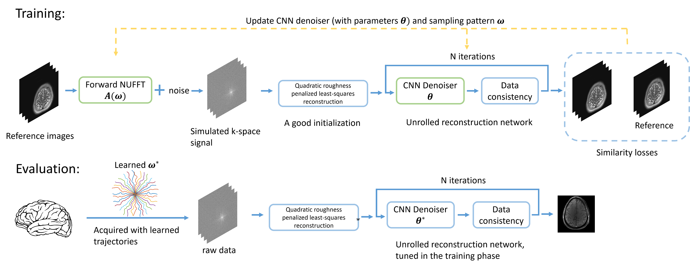
Figure 1: Diagram of the proposed approach. To optimize the sampling trajectory and the reconstruction algorithm jointly using a stochastic gradient descent (SGD)-type method, we construct a differentiable forward MRI system matrix $\bm{A}(\bm{\omega})$ that simulates k-space data w.r.t. trajectory $\bm{\omega}$ from ground truth images, and an unrolled neural network for reconstruction. The reconstruction errors compared with the ground truth are used as the training loss to update learnable parameters (the trajectory $\bm{\omega}$ and the network’s parameters $\bm{\theta}$).

2 Methods

This section describes the proposed approach for supervised learning of the sampling trajectory and image reconstruction method.

2.1 Problem formulation

Fig. 1 shows the overall workflow of the proposed approach. The goal is to optimize $\bm{\omega}\in\mathbb{R}^{N_{\mathrm{s}}\times N_{\mathrm{d}}}$, a trainable (possibly multi-shot) sampling pattern, and $\bm{\theta}\in\mathbb{R}^{M}$, the $M$ parameters of the image reconstruction method, where $N_{\mathrm{s}}$ denotes the total number of k-space samples, and $N_{\mathrm{d}}$ denotes the image dimensionality. (The results are for $N_{\mathrm{d}}=2$, i.e., 2D images, but the method is general.)

The training loss for jointly optimizing the trajectory parameters $\bm{\omega}$ and reconstruction parameters $\bm{\theta}$ is as follows:

$$\operatornamewithlimits{arg\,min}_{\bm{\omega}\in\mathbb{R}^{N_{\mathrm{s}}\times N_{\mathrm{d}}},\,\bm{\theta}\in\mathbb{R}^{M}}\mathbb{E}_{\bm{x}\in\mathcal{X}}[\ell(f_{\bm{\theta}}(\bm{\omega};\bm{A}(\bm{\omega})\bm{x}+\bm{\varepsilon}),\bm{x})]$$ (1)

s.t. $$\|\bm{D}_{1}\bm{\omega}^{[d]}\|_{\infty}\leq\gamma\Delta tg_{\max},$$

$$\|\bm{D}_{2}\bm{\omega}^{[d]}\|_{\infty}\leq\gamma\Delta t^{2}s_{\max},\ d=1,\ldots,N_{\mathrm{d}},$$

where each $\bm{x}\in\mathbb{C}^{N_{\mathrm{v}}}$ is a fully sampled reference image having $N_{\mathrm{v}}$ voxels drawn from the training data set $\mathcal{X}$ and $\bm{\varepsilon}$ is simulated additive complex Gaussian noise. (In practice the expectation is taken over mini-batches of training images.)

The system matrix $\bm{A}=\bm{A}(\bm{\omega})\in\mathbb{C}^{N_{\mathrm{s}}N_{\mathrm{c}}\times N_{\mathrm{v}}}$ represents the MR imaging physics (encoding), where $N_{\mathrm{c}}$ denotes the number of receiver coils. For multi-coil non-Cartesian acquisition, it is a non-Cartesian SENSE operator [35] that applies a pointwise multiplication of the sensitivity maps followed by a NUFFT operator (currently we do not consider field inhomogeneity but it would be straightforward to extend because the Jacobian approximation can cover such cases [33]). The function $f_{\bm{\theta}}(\bm{\omega};\cdot)$ denotes an image reconstruction algorithm with parameters $\bm{\theta}$ that is applied to simulated under-sampled data $\bm{A}(\bm{\omega})\bm{x}+\bm{\varepsilon}$. As detailed in subsection 2.3, we use an unrolled neural network. The reconstruction loss $\ell(\cdot,\cdot)$ quantifies the similarity between a reconstructed image and the ground truth, and can be a combination of different terms. Here we chose the loss $\ell$ to be a combined $\ell_{1}$ and square of $\ell_{2}$ norm. The matrices $\bm{D}_{1}$ and $\bm{D}_{2}$ denote the first-order and second-order finite difference operators. $\Delta t$ is the raster time and $\gamma$ denotes the gyromagnetic ratio. For multi-shot imaging, the difference operator applies to each shot individually. The optimization is constrained in gradient field strength ($g_{\max}$), and slew rate ($s_{\max}$). To use the stochastic gradient descent (SGD) method, we convert the box constraint into a penalty function $\bm{\phi}$, where

$$\bm{\phi}_{\lambda}(|\bm{x}|)=\bm{1}^{T}\max.(|\bm{x}|-\lambda,0),$$

where $\max.(\cdot)$ operates point-wisely. Our final joint optimization problem has the following form:

$$\operatornamewithlimits{arg\,min}_{\bm{\omega}\in\mathbb{C}^{N_{\mathrm{s}}\times N_{\mathrm{d}}},\,\bm{\theta}\in\mathbb{R}^{M}}\mathbb{E}_{\bm{x}\in\mathcal{X}}[ \,\ell(f_{\bm{\theta},\bm{\omega}}(\bm{\omega};\bm{A}(\bm{\omega})\bm{x}+\bm{\varepsilon}),\bm{x})]$$ (2)

$$+\mu_{1}\bm{\phi}_{\gamma\Delta tg_{\max}}(|\bm{D}_{1}\bm{\omega}|)$$

$$+\mu_{2}\bm{\phi}_{\gamma\Delta t^{2}s_{\max}}(|\bm{D}_{2}\bm{\omega}|).$$

We update $\bm{\theta}$ and $\bm{\omega}$ simultaneously for each mini-batch of training data.

2.2 Parameterization and multi-level optimization

We parameterize the sampling pattern with 2nd-order quadratic B-spline kernels:

$$\bm{\omega}^{[d]}=\bm{B}\bm{c}^{[d]},\ d=1,\ldots,N_{\mathrm{d}},$$ (3)

where $\bm{B}\in\mathbb{R}^{N_{\mathrm{s}}\times L}$ denotes the interpolation matrix, and $\bm{c}^{[d]}$ denotes the $d$th column of the coefficient matrix $\bm{c}\in\mathbb{R}^{L\times N_{\mathrm{d}}}$. $L$ denotes the length of $\bm{c}^{[d]}$, or the number of interpolation kernels in each dimension. The decimation rate in Fig. 5 is defined as $\text{Decim.}=N_{\mathrm{s}}/L$. Compared to other parameterization kernels, B-spline kernels reduce the number of individual inequality constraints (on maximum gradient strength and slew rate) from $4N_{\mathrm{d}}N_{\mathrm{s}}$ to $4N_{\mathrm{d}}L$ where typically $L\ll N_{\mathrm{s}}$. See [36] for more details.

Early versions of previous work [31] and our preliminary experiments found optimized trajectories that were often local minima near the initialization, only slightly perturbing the initial trajectory. We use a multilevel training strategy to improve the optimization process [37, 38].

We initialized the decimation rate $N_{\mathrm{s}}/L$ with a large value (like 64). Thus, many neighboring sample points are controlled by the same coefficient, which introduces more ‘non-local’ improvements. After both $\bm{c}$ and $\bm{\theta}$ converge, we reduce the decimation rate, typically by a factor of $2$, and begin a new round of training initialized with $\bm{\omega}$ and $\bm{\theta}$ of the previous round. Fig. 5 depicts the evolution along with decimation rates.

2.3 Reconstruction

In the joint learning model, we adopted a model-based unrolled neural network (UNN) approach to image reconstruction [34, 39, 40, 41]. Compared to the previous joint learning model (PILOT) that used a single image domain network [31], an unrolled network can lead to a more accurate reconstruction [34], at the price of longer reconstruction time.

A typical cost function for regularized MR image reconstruction has the form:

$$\hat{\bm{x}}=\operatornamewithlimits{arg\,min}_{\bm{x}}\|\bm{A}\bm{x}-\bm{y}\|_{2}^{2}+\mathcal{R}(\bm{x}).$$ (4)

The first term is usually called the data-consistency term that ensures the reconstructed image is consistent with the acquired k-space data $\bm{y}$. (In the training phase, $\bm{A}(\bm{\omega})\bm{x}+\bm{\varepsilon}$ is the simulated $\bm{y}$.) The regularization term $\mathcal{R}(\cdot)$ is designed to control aliasing and noise when the data is under-sampled. By introducing an auxiliary variable $\bm{z}$, one often replaces (4) with the following alternative:

$$\hat{\bm{x}}=\operatornamewithlimits{arg\,min}_{\bm{x}}\min_{\bm{z}}\|\bm{A}\bm{x}-\bm{y}\|_{2}^{2}+\mathcal{R}(\bm{z})+\mu\|\bm{x}-\bm{z}\|_{2}^{2},$$ (5)

where $\mu>0$ is a penalty parameter. Using an alternating minimization approach, the optimization updates become:

$$\bm{x}_{i+1}=\operatornamewithlimits{arg\,min}_{\bm{x}}{\|\bm{A}\bm{x}-\bm{y}\|_{2}^{2}+\mu\|\bm{x}-\bm{z}_{i}\|_{2}^{2}},$$ (6)

$$\bm{z}_{i+1}=\operatornamewithlimits{arg\,min}_{\bm{z}}{\mathcal{R}(\bm{z})+\mu\|\bm{x}_{i+1}-\bm{z}\|_{2}^{2}}.$$ (7)

The analytical solution for the $\bm{x}$ update is

$$\bm{x}_{i+1}=(\bm{A}^{\prime}\bm{A}+\mu\bm{I})^{-1}(\bm{A}^{\prime}\bm{y}+\mu\bm{z}_{i}),$$

which involves a matrix inverse that would be computationally prohibitive to compute directly. Following [34], we use a few iterations of the conjugate gradient (CG) method for the $\bm{x}$ update. The implementation uses a Toeplitz embedding technique to accelerate the computation of $\bm{A}^{\prime}\bm{A}$ [42, 43].

For a mathematically defined regularizer, the $\bm{z}$ update would be a proximal operator. Here we follow previous work [44, 34] and use a CNN-based denoiser $\bm{z}_{i+1}=\mathcal{D}_{\bm{\theta}}(\bm{x}_{i+1})$. To minimize memory usage and avoid over-fitting, we used the same $\bm{\theta}$ across iterations, though iteration-specific networks may improve the reconstruction result [41].

For the CNN-based denoiser, we used the Deep Iterative Down-Up CNN (DIDN) [45, 41]. As a state-of-art model for image denoising, the DIDN model requires less memory than popular models like U-net [32] while providing improved reconstruction results. In our experiments, it also led to faster training convergence than previous denoising networks.

Since neural networks are sensitive to the scale of the input, a good and consistent initial estimate of $\bm{x}$ is important. We used the following quadratic roughness penalty approach to compute an initial image estimate:

$$\bm{x}_{0} =\operatornamewithlimits{arg\,min}_{\bm{x}}{\|\bm{A}\bm{x}-\bm{y}\|_{2}^{2}+\lambda\|\bm{R}\bm{x}\|_{2}^{2}}$$ (8)

$$=(\bm{A}^{\prime}\bm{A}+\lambda\bm{R}^{\prime}\bm{R})^{-1}\bm{A}^{\prime}\bm{y},$$

where $\bm{R}$ denotes the $N_{\mathrm{d}}$-dimensional first-order finite difference (roughness) operator. We also used the CG method to (approximately) solve this quadratic minimization problem.

2.4 Correction of eddy-current effect

Rapidly changing gradient waveforms may suffer from eddy-current effects, even with shielded coils. This hardware imperfection requires additional measurements and corrections so that the actual sampling trajectory is used for reconstructing real MRI data. Some previous works used a field probe and corresponding gradient impulse-response (GIRF) model [46]. In this work, we adopted the ‘k-space mapping’ method [47, 8] that does not require additional hardware. Rather than mapping the $k_{x}$ and $k_{y}$ components separately as in previous papers, we excited a pencil-beam region using one $90^{\circ}$ flip and a subsequent $180^{\circ}$ spin-echo pulse [48]. We averaged multiple repetitions to estimate the actual acquisition trajectory. We also subtracted a zero-order eddy current phase term from the acquired data [8].

The following pseudo-code summarizes the BJORK training process.

Algorithm 1 Training algorithm for BJORK

1:Training set $\mathcal{X}$; denoiser $\mathcal{D}_{\bm{\theta}}$ for initial CNN weights $\bm{\theta}_{0}$; initial trajectory $\bm{\omega}_{0}$; levels of optimization $N_{\mathrm{level}}$; number of epoch $N_{\mathrm{epoch}}$; step size of denoiser update $\eta_{\mathcal{D}}$; step size of trajectory update $\eta_{\bm{\omega}}$; penalty parameter for gradient/slew rate constraint $\mu_{1}$ and $\mu_{2}$.

2:$\bm{\omega}=\bm{B}\bm{c}$

3:$\bm{\theta}\leftarrow\bm{\theta}_{0}$

4:$\bm{\omega}\leftarrow\bm{\omega}_{0}$

5:Pre-train $\mathcal{D}_{\bm{\theta}}$ with fixed $\bm{\omega}_{0}$.

6:for $l$ = 1 to $N_{\mathrm{level}}$ do

7:     Initialize new coefficient matrix $\bm{B}_{l}$.

8:     Initialize new coefficient $\bm{c}_{l}^{0}$ with $\bm{\omega}_{l-1}\approx\bm{B}_{l}\bm{c}_{l}^{0}$.

9:     for $j$ = 1 to $N_{\mathrm{epoch}}$ do

10:         for training batches $\bm{x}^{K}$ in $\mathcal{X}$ do

11:              Simulate the k-space w.r.t. $\bm{\omega}_{l}$:

12:              $\bm{y}^{K}=\bm{A}(\bm{\omega}_{l}^{K})\bm{x}^{K}+\bm{\varepsilon}$

13:              Reconstruction with UNN:

14:              Reconstruct initial images using (8) with CG

15:              for $i$ = 1 to $N_{\mathrm{iter}}$ do

16:                  $\bm{x}_{i+1}$: UNN reconstruction update of $\bm{z}_{i}$

17:                      using (6)

18:                  Apply CNN: $\bm{z}_{i+1}=\mathcal{D}_{\bm{\theta}}(\bm{x}_{i+1})$

19:              end for

20:              Calculate loss function:

21:              $L=\ell(\hat{\bm{x}}^{K},\bm{x}^{K})+\mu_{1}\bm{\phi}_{\gamma\Delta tg_{\max}}(|\bm{D}_{1}\bm{\omega}_{i}^{K}|)$

22:              $\quad\mbox{}+\mu_{2}\bm{\phi}_{\gamma\Delta t^{2}s_{\max}}(|\bm{D}_{2}\bm{\omega}_{i}^{K}|)$

23:              Update denoiser and trajectory:

24:              $\bm{\theta}^{K}=\bm{\theta}^{K-1}-\eta_{\mathcal{D}}\nabla_{\bm{\theta}^{K-1}}L$

25:              $\bm{\omega}_{l}^{K}=\bm{\omega}_{l}^{K-1}-\eta_{\bm{\omega}}\nabla_{\bm{\omega}_{l}^{K-1}}L$

26:         end for

27:     end for

28:end for

3 Experiments

Table 1: Protocols for data acquisition

Protocols for the prospective experiment:
Name	FOV(cm)	dz(mm)	Gap(mm)	TR(ms)	TE(ms)	FA	Acqs	dt(us)	Time
Radial-like	22*22*4	2	0.5	318.4	3.56	90°	32*1280	4	0:11
Radial-full	22*22*4	2	0.5	318.4	3.56	90°	320*1280	4	1:40
dz: slice thickness; Gap: gap between slices; Acqs: number of shots * readout points; FA: flip angle

3.1 Comparison with prior art

We compared the proposed BJORK approach with the SPARKLING method for trajectory design in all experiments, and have set the readout length and physical constraints to be the same for both methods.

Both BJORK and PILOT [31] are methods for joint sampling design and reconstruction optimization. We compared three key differences between the two methods individually. (1) The NUFFT Jacobian matrices, as discussed in [33] and the Appendix. (2) The reconstruction method involved. Our BJORK approach uses an unrolled neural network, while PILOT uses a single reconstruction neural network in the image domain (U-Net). We also presented the effect of trajectory parameterization (BJORK uses quadratic B-splines following [36], whereas versions 1-3 of PILOT used no parameterization and more recent versions of PILOT use cubic splines [31]).

3.2 Image quality evaluation

To evaluate the reconstruction quality provided by different trajectories, we used two types of reconstruction methods in the test phase: unrolled neural network (UNN) (with learned $\bm{\theta}$) and a compressed sensing approach (sparsity regularization for an discrete wavelet transform). For SPARKLING-optimzed trajectories and standard undersampled trajectories (radial/spiral), we used the same unrolled neural networks as in BJORK for reconstruction. Only the network parameters $\bm{\theta}$ were trained, with the trajectory $\bm{\omega}$ fixed.

We also used compressed sensing-based reconstruction to test the generalizability of BJORK-optimized trajectories. The penalty function is the $\ell_{1}$ norm of a discrete wavelet transform with a Daubechies 4 wavelet. The ratio between the penalty term and the data-fidelity term is $10^{-7}$. We used the SigPy package and its default primal-dual hybrid gradient (PDHG) algorithm (with 50 iterations). This study includes two evaluation metrics: the structural similarity metric (SSIM) and peak signal-to-noise ratio (PSNR) [49].

3.3 Trajectories

For both simulation and real acquisition, the acquisition sampling time and gradient raster time are both 4 $\mu$s, with a target matrix size of 320$\times$320. The maximum gradient strength is 26.7 mT/m, and the maximum slew rate is 150 T/m/s, which were set to limit peripheral nerve stimulation and conform to the Nyquist criterion.

To demonstrate the proposed model’s adaptability, we investigated two types of initialization of waveforms: an undersampled in-out radial trajectory with a shorter readout time ($\sim$5 ms) and an undersampled center-out spiral trajectory with a longer readout time ($\sim$16 ms). For the in-out radial initialization, the number of spokes is 16/24/32, and each spoke has 1280 points of acquisition (4 $\mu$s samples). The rotation angle is equidistant between $-\pi/2$ and $\pi/2$. For the center-out spiral initialization, the number of spokes is 8, and each leaf has $\sim$4000 points of acquisition. We used the variable-density spiral design package from [50]. For SPARKLING, we use $\tau=0.5$ and $d=2.5$ for 16-spoke radial, $\tau=0.5$ and $d=2.5$ for 24-spoke radial, $\tau=0.6$ and $d=2.5$ for 32-spoke radial, and $\tau=0.5$ and $d=2$ for 8-shot spiral ([15, Eqn. 8], which can also be learned as described in [51].) after grid search with CS-based reconstruction.

3.4 Network training and hyper-parameter setting

The simulation experiments used the NYU fastMRI brain dataset to train the trajectories and neural networks [52]. The dataset consists of multiple contrasts, including T1w (23220 slices), T2w (42250 slices), and FLAIR (5787 slices). FastMRI’s knee subset was also used in a separate training run to investigate the influence of training data on learned sampling patterns. The central $320\times 320$ region was cropped (or zero-filled). Sensitivity maps were estimated using the ESPIRiT method [53] with the central 24 phase-encoding lines, and the corresponding conjugate phase reconstruction was regarded as the ground truth during training.

The batchsize was 4. The number of blocks, or the number of outer iterations for the unrolled neural network was 6. The weight $\mu$ in (5) could also be learned, but this operation would double the computation load with minor improvement. We set $\mu=2$. The number of training epochs was set to 3 for each level of B-spline kernel length, which is empirically enough for the training to converge. We used $N_{\mathrm{level}}=4$ optimization levels, and $N_{\mathrm{epoch}}=3$ so the total number of epochs was 12. We set $N_{\mathrm{iter}}=6$ of the unrolled neural network. For training the reconstruction network with existing trajectories (radial, spiral, and SPARKLING-optimized), we also used 12 training epochs. We used the Adam optimizer [54], with parameter $\bm{\beta}$ = $[0.5,0.999]$, for both trajectories $\bm{\omega}$ and network parameters $\bm{\theta}$. The learning rate linearly decayed from 1e-3 to 0 for the trajectory update, and from 1e-5 to 0 for the network update. We did not observe obvious over-fitting phenomena on the validation set. The training on a Intel Xeon Gold 6138 CPU and an Nvidia RTX2080Ti GPU took around 120-150 hours.

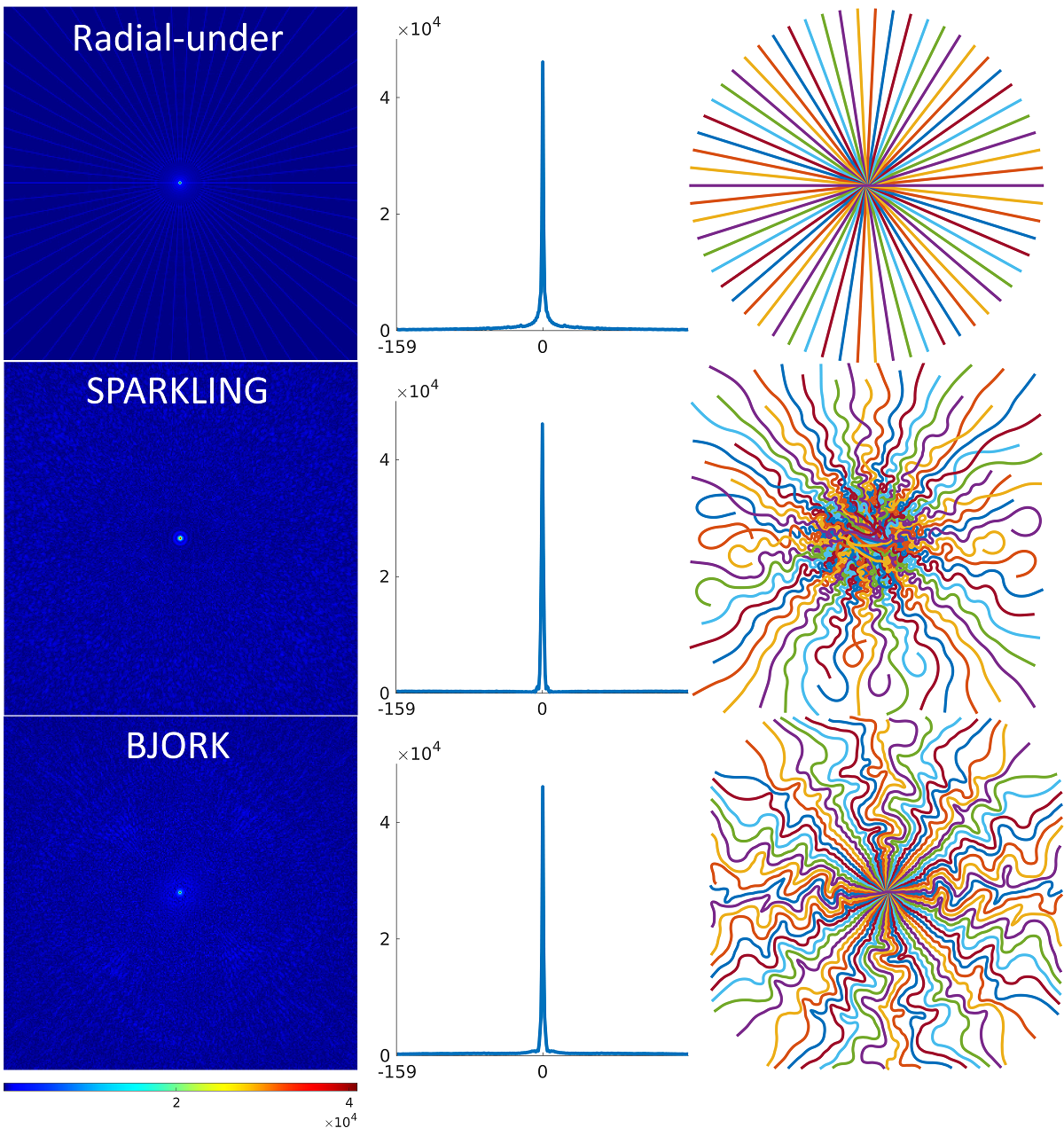
Figure 2: PSFs of different sampling patterns. Each middle plot is the averaged profile of different views (angles) through the origin. The FWHM for undersampled radial, BJORK and SPARKLING is respectively 1.5, 1.6, 2.1 pixels.

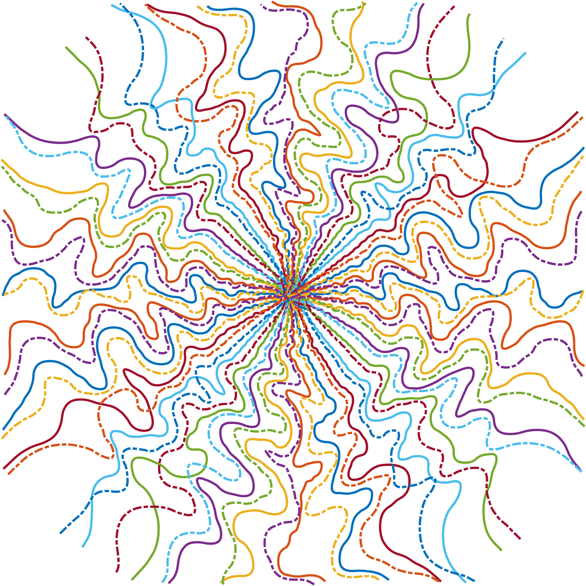
Figure 3: The dash-dot line shows the $180^{\circ}$ rotated BJORK trajectory. The original and rotated trajectory have little overlap, suggesting that the BJORK automatically learned a sampling pattern that exploits approximate k-space Hermitian symmetry.

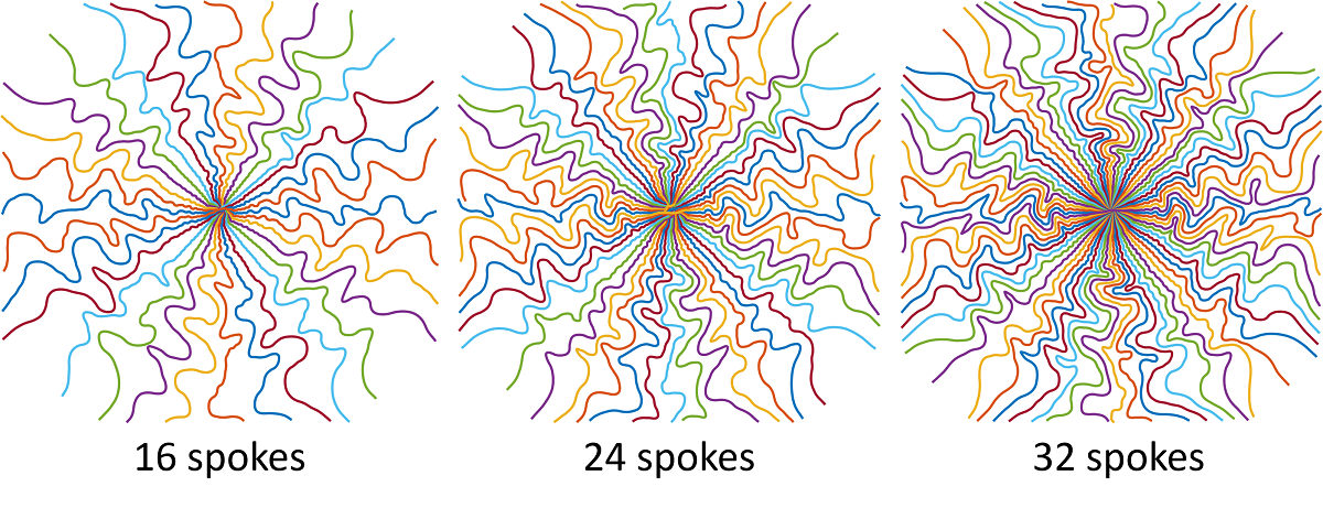
Figure 4: Learned radial-like trajectories with different acceleration ratios.

3.5 Prospective Studies

Table 1 details the scanning protocols of the RF-spoiled, gradient echo (GRE) sequences used. For in-vivo acquisitions, a fat-saturation pulse was applied before the tip-down RF pulse. We chose the TR and FA combination for desired T1-weighed contrast. For radial-like sequences, we tested a GRE sequence with 3 different readout trajectories: standard undersampled radial, BJORK initialized with undersampled radial, and SPARKLING initialized with undersampled radial. Radial-full means the fully sampled radial trajectory. The simulation experiments (evaluation) and real experiments use the same readout trajectory.

We also acquired an additional dual-echo Cartesian GRE image, for generating the sensitive map and (potentially) B0 map. The sensitivity maps were generated by ESPIRiT [53] methods. The sequences were programmed with TOPPE [48], and implemented on a GE MR750 3.0T scanner with a Nova Medical 32 channel Rx head coil. Subjects gave informed consent under local IRB approval. For phantom experiments, we used a water phantom with 3 internal cylinders.

The k-space mapping was implemented on a water phantom. The thickness of the pencil-beam was $2$mm $\times$ $2$mm. The trajectory estimates were based on an average of 30 repetitions.

4 Results

4.0.1 Quantitative results of simulation reconstruction study

The test set includes 1520 slices, and the validation set includes 500 slices. Table 2 shows the quantitative results (SSIM and PSNR). The proposed method has significant improvement compared with un-optimized trajectories ($P<0.005$). It also has improved reconstruction quality compared with SPARKLING considering unrolled neural network-based reconstruction. Compared to undersampled radial trajectory or SPARKLING trajectory, the proposed method has a better restoration of details and lower levels of artifacts. In the experiment, different random seeds in training led to very similar learned sampling trajectories.

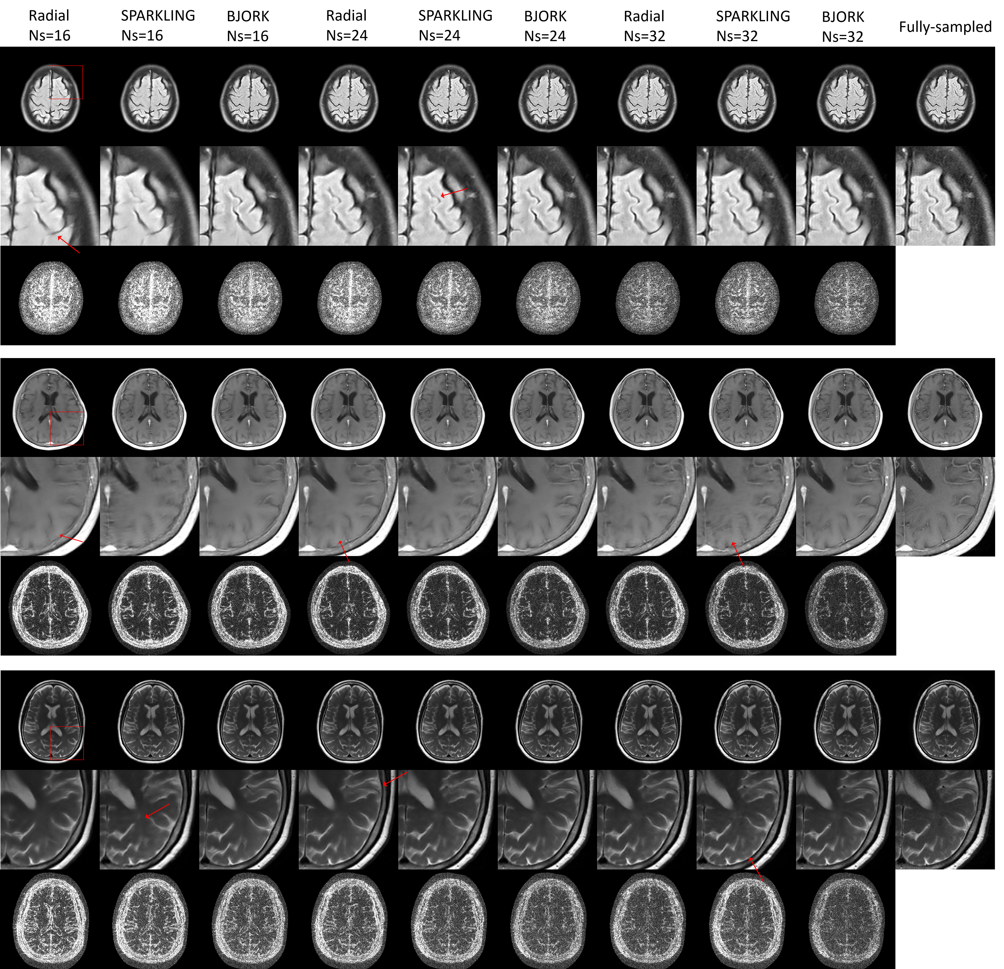
Figure 11: Examples from the simulation experiment using the UNN-based reconstruction algorithm, with three different acceleration ratios. Ns stands for the number of shots or spokes. The first slice is FLAIR contrast. The second slice is T1w contrast. The third slice T2w contrast. Red boxes indicate the zoom-in region, and red arrows point to reconstruction artifacts/blur. Below the zoomed-in regions are the corresponding error maps, compared with fully sampled images.

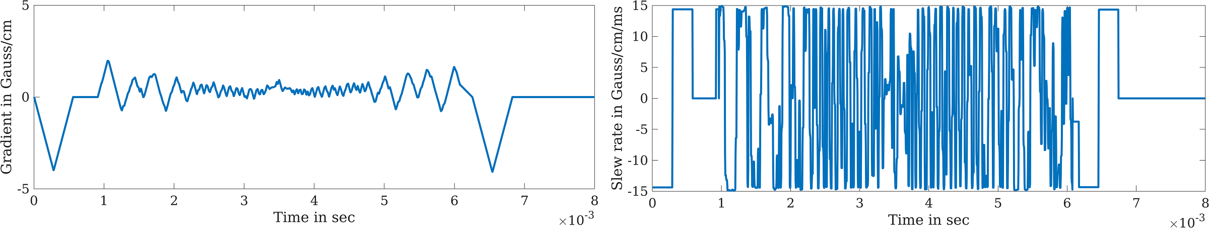
Figure 12: The gradient strength and slew rate of one spoke from BJORK-optimized radial trajectory.

Fig. 2 displays point spread functions of 32-spoke radial-like trajectories. The BJORK’s PSF has a narrower central-lobe than SPARKLING and much fewer streak artifacts than standard radial. Fig. 3 shows the conjugate symmetry relationship implicitly learned in the BJORK trajectory. Fig. 4 displays optimization results under different acceleration ratios. Fig. 11 in the Appendix exhibits example slices. Fig. 12 in the Appendix shows the gradient waveform of one shot on one direction (from the optimized 32-spoke radial-like trajectory) and the corresponding slew rate.

Table 2: Quantitative results for simulation experiments

SSIM:
		Standard	SPARKLING	BJORK
radial-like Ns=16	UNN	0.940	0.946	0.950
	CS	0.911	0.936	0.938
radial-like Ns=24	UNN	0.950	0.955	0.959
	CS	0.929	0.943	0.948
radial-like Ns=32	UNN	0.957	0.963	0.968
	CS	0.932	0.946	0.956
spiral-like Ns=8	UNN	0.986	0.989	0.990
	CS	0.976	0.978	0.981

PSNR (in dB):
		Standard	SPARKLING	BJORK
radial-like Ns=16	UNN	32.7	33.9	34.3
	CS	31.7	33.6	34.1
radial-like Ns=24	UNN	34.1	35.0	35.6
	CS	33.3	34.6	35.1
radial-like Ns=32	UNN	35.0	36.0	36.9
	CS	33.9	35.7	36.3
spiral-like Ns=8	UNN	40.9	41.7	41.9
	CS	39.9	40.4	40.7
Ns: the number of shots or spokes.

4.0.2 Multi-level optimization

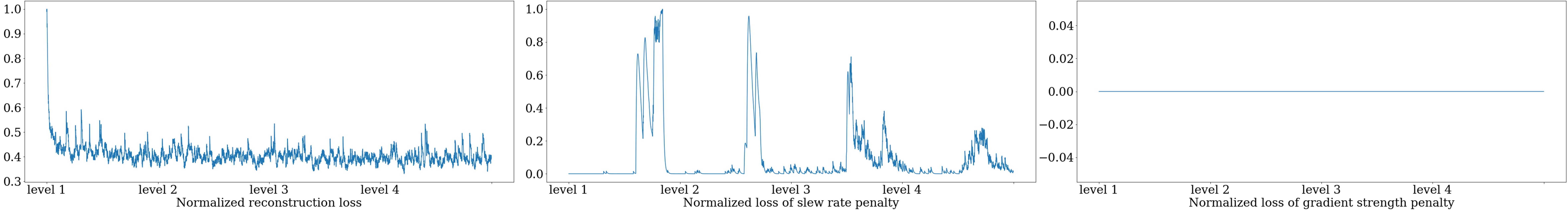
Figure 13: Smoothed training training losses of a 16-spoke radial-initialized sequence. We use 4 levels and each level contains 3 epochs. The three columns are the reconstruction loss, penalty on the maximum slew rate, and penalty on the maximum gradient strength.

Fig. 5 shows the evolution of sampling patterns using our proposed multi-level optimization. Different widths of the B-spline kernels introduce different levels of improvement as the acquisition is optimized. Also shown are the results of multi-level optimization and a nonparametric trajectory as used early versions of the PILOT paper [31, versions 1-3]. Directly optimizing sampling points seems only to introduce a small perturbation to the initialization. Fig. 13 in the Appendix shows the training losses: the reconstruction loss $\ell(\cdot,\cdot)$, the penalty on maximum gradient strength, and the penalty on maximum slew rate. Transitions between different B-spline kernel widths led to a stepped training loss descent pattern.

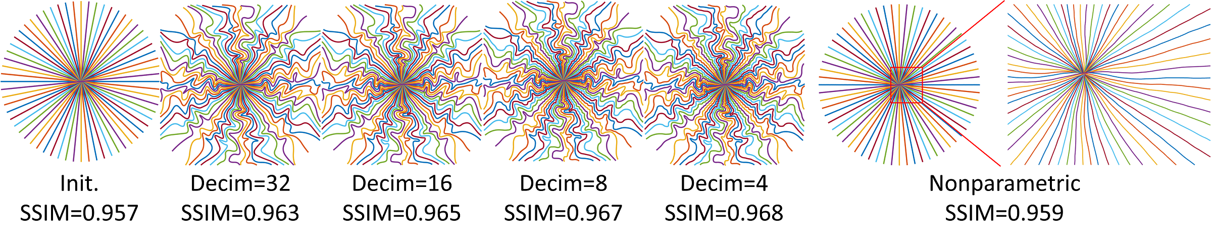
Figure 5: The evolution of the learned trajectories. Decim means $N_{\mathrm{s}}/L$ in (3). Nonparametric means the locations of each sampling points are independent trainable variables, rather than being parameterized by quadratic B-spline kernels. SSIM denotes the average reconstruction quality on the evaluation set of each level. The rightmost zoomed-in set shows the very small perturbations produced by the nonparametric approach (stuck into local-minima).

4.0.3 Effect of training set

Fig. 6 shows radial-initialized trajectories trained by BJORK with brain and knee datasets. Different trajectories are learned from different datasets. We hypothesize that the difference is related to frequency distribution of energy, as well as the noise level, which requires further study. This phenomenon was also observed in [22].

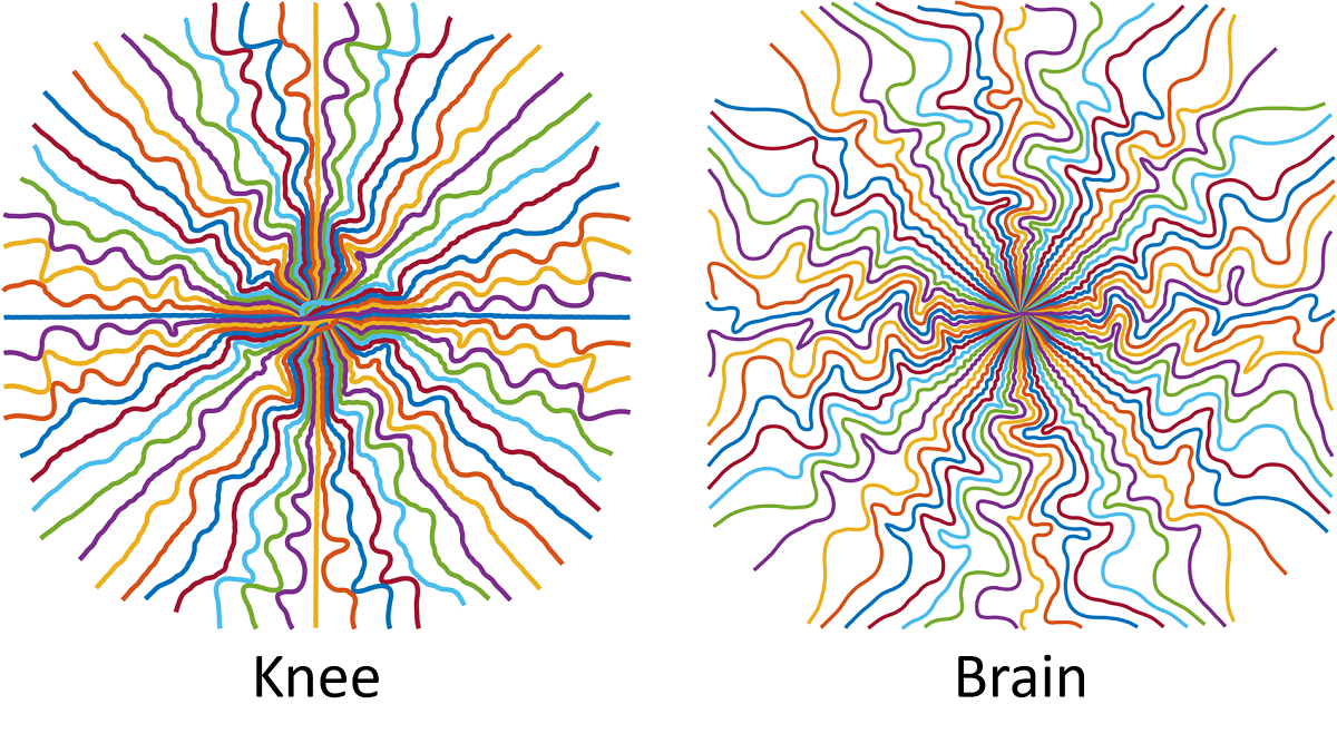
Figure 6: Trajectories learned from different datasets.

4.0.4 Effect of reconstruction methods

To test the influence of reconstruction methods on trajectory optimization, we tried a single image-domain refinement network as the reconstruction method in the joint learning model, similar to PILOT’s approach. Quadratic roughness penalty reconstruction in (8) still is the network’s input. The initialization of the sampling pattern is an undersampled radial trajectory. Table 3 shows that the proposed BJORK reconstruction method (unrolled neural network, UNN) improves reconstruction quality compared to a single end-to-end model. Such improvements are consistent with other comparisons between UNN methods and image-domain CNN methods using fixed sampling patterns (reconstruction only) [39, 34, 41].

Table 3: Effect of different reconstruction networks involved in the joint learning model

	SSIM	PSNR(dB)
UNN	0.968	36.9
Single U-net	0.934	32.8

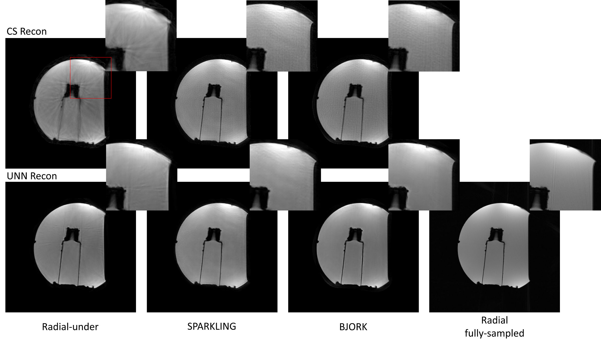
Figure 7: Representative results of the prospective phantom experiment using CS-based and UNN-based reconstruction algorithms. The sequences involved were radial-like GRE (detailed in Table 1) with T1w contrast. The parameters of UNNs are trained with fastMRI dataset without fine-tuning. The readout length was 5.12 ms. The number of shots for undersampled trajectories was 32, and for the fully-sampled radial trajectory is 320 ($10\times$ acceleration). The FOV was 22cm. Red boxes indicate the zoomed-in regions displayed on the upper right corner.

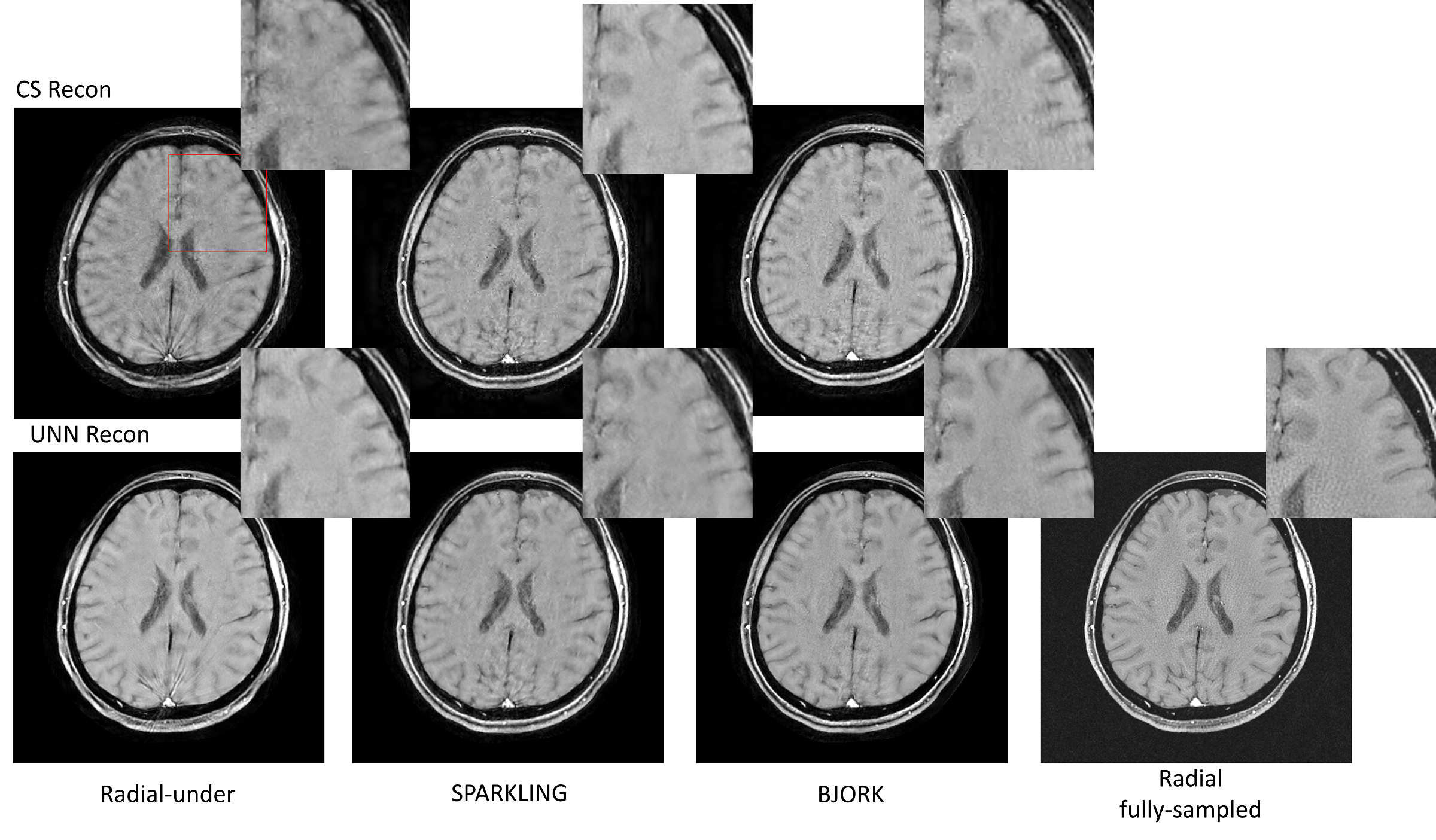
Figure 8: Results of the T1w prospective in-vivo experiment. The trajectories were also radial-like (detailed in Table 1). The parameters of UNNs are trained with the fastMRI dataset without fine-tuning. The readout time was 5.12 ms. The number of shots for undersampled trajectories was 32, and for the fully-sampled radial trajectory is 320 ($10\times$ acceleration). The FOV was 22cm. Red boxes indicate the zoomed-in regions displayed on the upper right corner.

4.0.5 Prospective experiments

Fig. 7 shows the water phantom results for different reconstruction algorithms. The rightmost column is the fully-sampled ground truth (Radial-full). Note that the unrolled neural network (UNN) here was trained with fastMRI brain dataset, and did not receive fine-tuning in all prospective experiments. The BJORK-optimized trajectory leads to fewer artifacts and improved contrast for the UNN-based reconstruction.

Fig. 8 showcases one slice from the in-vivo experiment. For CS-based reconstruction, the undersampled radial trajectory exhibits stronger streak artifacts than SPARKLING- and BJORK-optimized trajectories. For UNN-based reconstruction, all trajectories’ results show reductions of artifacts compared to CS-based reconstruction. The proposed method restores most of the structures and fine details, with minimal artifacts.

The Appendix also contains examples of reconstruction results before/after eddy currents correction, the measurement of actual k-space trajectories, and effectiveness of the warm initialization (quadratic least-squares reconstruction).

5 Discussion

This paper proposes an efficient learning-based framework for the joint design of MRI sampling trajectories and reconstruction parameters. Defining an appropriate objective function for trajectory optimization is an open question. We circumvented this long-lasting problem by directly using the reconstruction quality as the training loss function in a supervised learning paradigm. The workflow includes a differentiable reconstruction algorithm for which the learning process obtains an intermediate gradient w.r.t. the reconstruction loss. However, solely depending on backpropagation and stochastic gradient descent cannot guarantee optimal results for this non-convex problem. To improve the training effect, we adopted several techniques, including trajectory parameterization, multi-level training, warm initialization of the reconstruction network, and an accurate approximation of NUFFT’s Jacobian [33]. Results show that these approaches can stabilize the training and provide better local minimizers than previous methods.

We trained an unrolled neural network-based reconstruction method for non-Cartesian MRI data. The single image-domain network used in previous work does not efficiently remove aliasing artifacts. Additionally, the k-space “hard” data-consistency trick for data fidelity [55, 56] is inapplicable for non-Cartesian sampling. An unrolled algorithm can reach a balance between data fidelity and the de-aliasing effect across multiple iterations. For 3D trajectory design using the proposed approach, the unrolled method’s memory consumption can be huge. More memory-efficient reconstruction models, such as the memory-efficient network [57] should be explored in further study. We would also investigate recent calibration-less unrolled neural networks, which do not require external sensitivity maps, and shows improved performance relative to MoDL [58].

For learning-based medical imaging algorithms, one main obstacle towards clinical application is the gap between simulation and the physical world. Some factors include the following.

First, inconsistency exists between the training datasets and real-world acquisition, such as different vendors and protocols, posing a challenge to reconstruction algorithms’ robustness and generalizability. Our training dataset consisted of T1w/T2w/FLAIR Fast Spin-Echo (FSE or TSE) sequences, acquired on Siemens 1.5T/3.0T scanners. The number of receiver channels includes 4, 8, and 16, etc. We conducted the in-vivo/phantom experiment on a 3.0T GE scanner equipped with a 32-channel coil. The sequence is a GRE sequence that has lower SNR compared to FSE sequences in the training set. Despite the very large differences with the training set, our work still demonstrated improved and robust results in the in-vivo and phantom experiment, without any fine-tuning.

We hypothesize that several factors could contribute to the generalizability: (1) the reconstruction network uses the quadratic roughness penalized reconstruction as the initialization, normalized by the median value. Previous works typically use the adjoint reconstruction as the input of the network. In comparison, our regularized initialization helps provide consistency between different protocols, without too much compromise of the computation time/complexity, (2) the PSF of the learned trajectory has a compact central lobe, without significant streak artifacts. Thus the reconstruction is basically a de-blurring/denoising task that is a local low-level problem and thus may require less training data than de-aliasing problems. For de-blurring of natural images, networks are usually adaptive to different noise levels and color spaces, and require small cohorts of data [59, 60]. For trajectories like radial and SPARKLING, in contrast, a reconstruction CNN needs to remove global aliasing artifacts, such as the streak and ringing artifacts. The dynamics behind the neural network’s ability to resolve such artifacts is still an unsolved question, and the training requires a large amount of diverse data.

Secondly, it is not easy to simulate system imperfections like eddy currents and off-resonance in the training phase. These imperfections can greatly affect image quality in practice. We used a trajectory measurement method to correct for the eddy-current effect. Future work will incorporate field inhomogeneity into the workflow.

Furthermore, even though the BJORK sampling was optimized for a UNN reconstruction method, the results in Fig. 7 and Fig. 8 suggest that the learned trajectory is also useful with a CS-based reconstruction method or other model-based reconstruction algorithms. This approach can still noticeably improve the image quality by simply replacing the readout waveform in the existing workflow, promoting the applicability of the proposed approach, similar to [22]. We plan to apply the general framework to optimize a trajectory for (convex) CS-based reconstruction and compare to the (non-convex) open-loop UNN approach in future work.

Though the proposed trajectory is learned via a data-driven approach, it can also reflect the ideas behind SPARKLING and Poisson disk sampling: sampling patterns having large gaps or tight clusters of points are inefficient, and the sampling points should be somewhat evenly distributed (but not too uniform). Furthermore, BJORK appears to have learned some latent characteristics, like the conjugate symmetry for these spin-echo training datasets. To combine both methods’ strengths, a promising future direction is to use SPARKLING as a primed initialization of BJORK.

The learning used here exploited a big public data set. As is shown in the results, knee imaging and brain imaging led to different learned trajectories. This demonstrates that the data set can influence the optimization results, as was observed in [22]. We also implemented a complementary experiment on a smaller training set (results not shown). We found that a small subset (3000 slices) also led to similar learned trajectories. Therefore, for some organs where a sizeable dataset is not publicly available, this approach may still work with small-scale private datasets. To examine the influence of scanner models, field strength, and sequences, follow-up studies should investigate more diverse datasets.

The eddy-current effect poses a long-term problem for non-Cartesian trajectories and impedes their widespread clinical use. This work used a simple k-space mapping technique as the correction method. The downside of this method is its long calibration time, although it can be performed in a scanner’s idle time. This method is waveform-specific, which means that correction should be done for different trajectories. Other methods relying on field probes can get a more accurate correction with less time, albeit with dedicated hardware. In a future study, the eddy current-related artifacts could be simulated according to the GIRF model in the training phase, so that the trajectory is learned to be robust against the eddy current effect.

Aside from practical challenges with GPU memory, the general approach described here is readily extended from 2D to 3D sampling trajectories [16]. A more challenging future direction is to extend the work to dynamic imaging applications like fMRI and cardiac imaging, where both the sampling pattern and the reconstruction method should exploit redundancies in the time dimension, e.g., using low-rank models [61]. To optimize sampling in higher dimensions, the proposed approach should also have additional regularization on the PNS effect.

Appendix A Experiments

A.1 Eddy-current effect

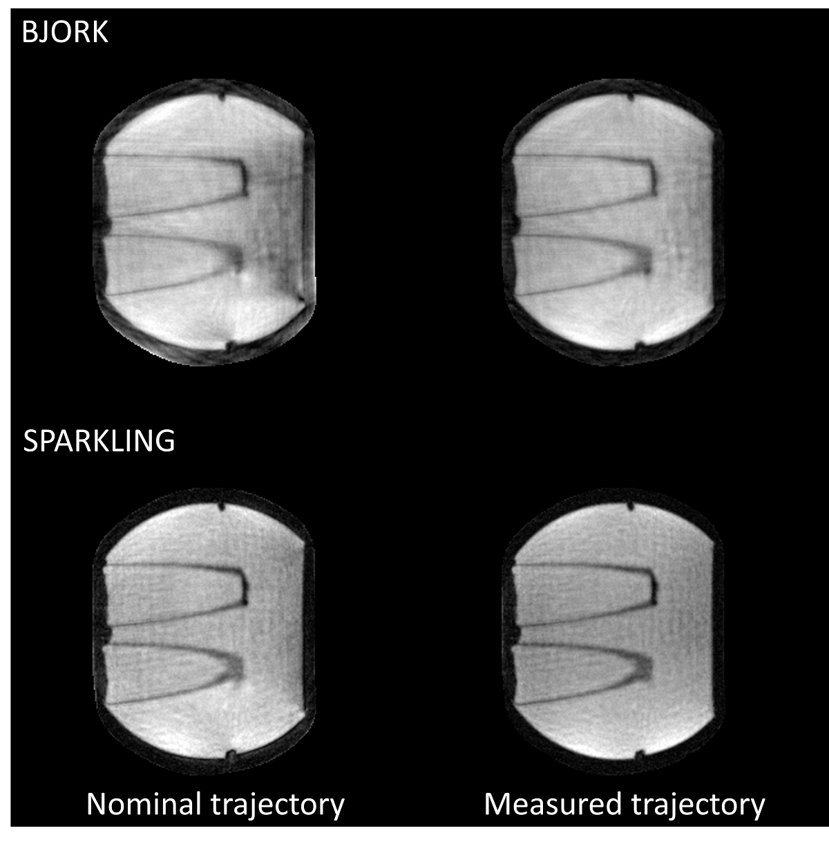
Figure 9: Compressed sensing-based reconstruction of a water phantom. The left column is the reconstruction with the nominal trajectory, and right is with the measured trajectory. Reconstruction with the mapped trajectory introduces fewer artifacts.

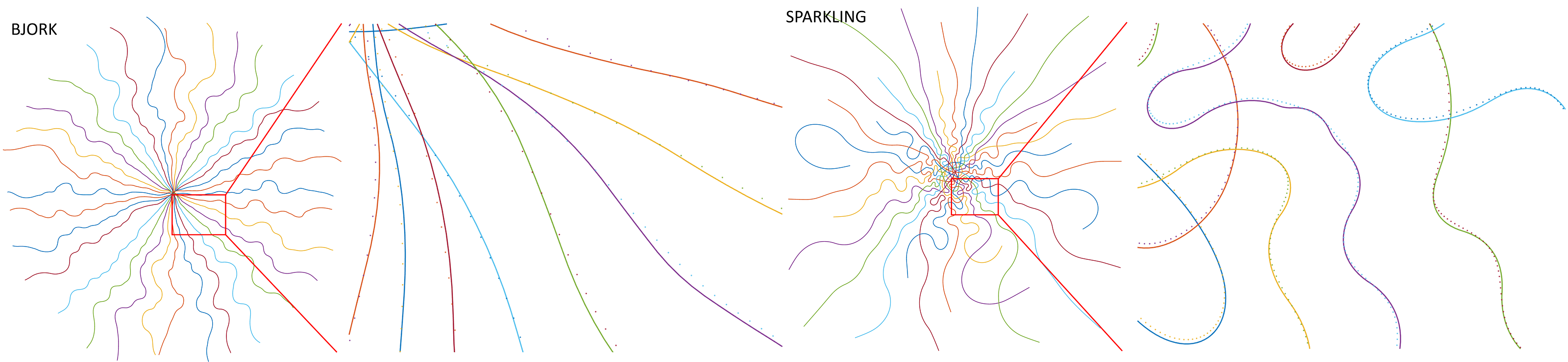
Figure 10: The measurement of the influence of the eddy currents on readout waveform. The solid line is the nominal trajectory, and the dotted line is the measurement.

Fig. 9 displays the CS-based reconstruction of real acquisitions reconstructed using both the nominally designed trajectories and the measured trajectories.

Fig. 10 shows the results of the trajectory measurements. Using the measurement of the actual trajectory seems to mitigate the influence of eddy current effects in the reconstruction results.

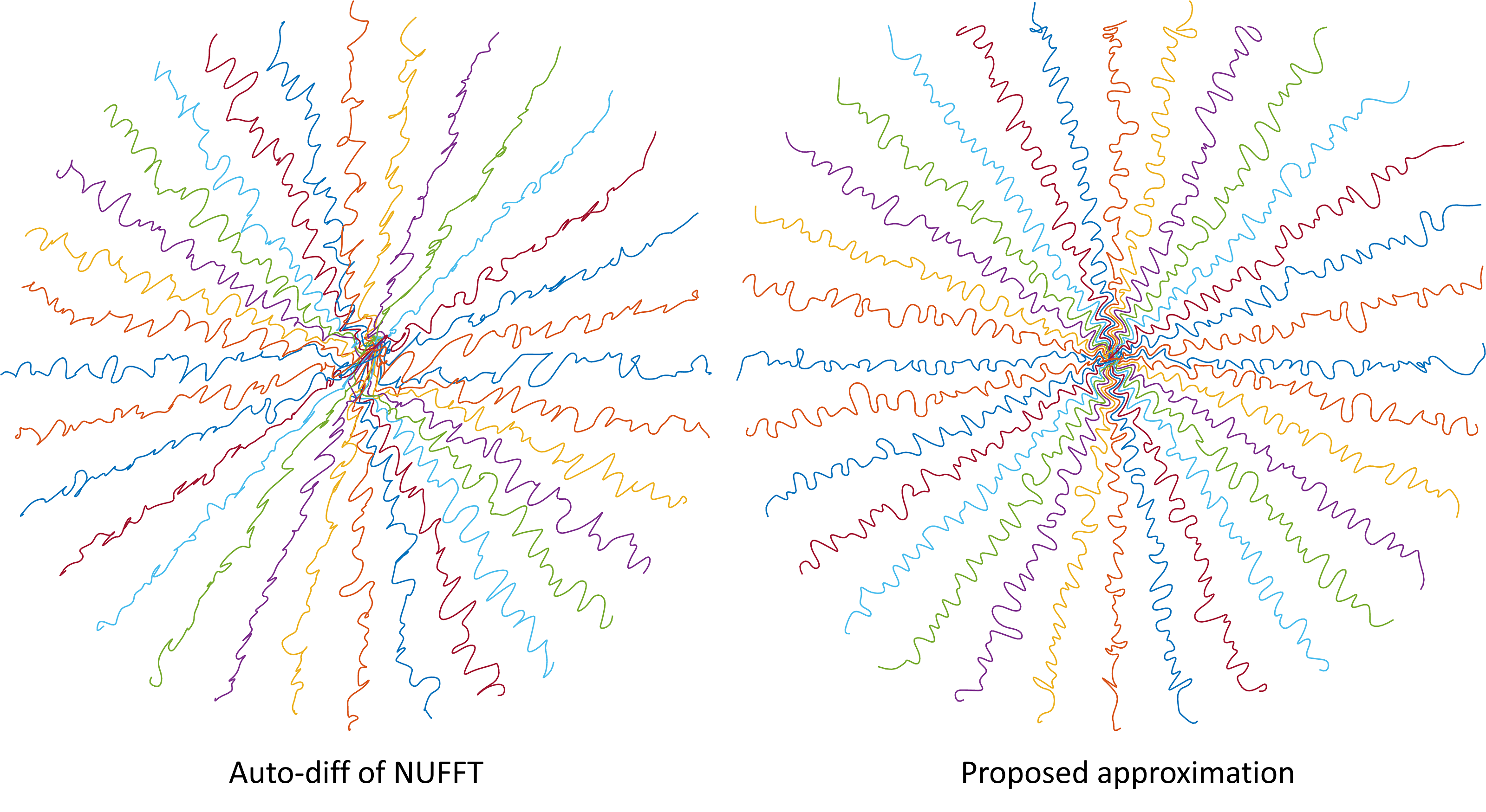
Figure 14: The learned trajectories with descent directions calculated by different methods.

A.2 Cross contrast validation

In this experiment, we trained the model with one image contrast from the fastMRI brain dataset (without simulated additive noise), and tested the learned trajectory with all contrasts (with simulated additive Gaussian noise whose variance is $10^{-3}$ of the mean magnitude of the signal). Each contrast has 4500 training slices and 500 test slices. We fine-tuned the reconstruction unrolled neural network for different test contrasts. The initialization is a 16-spoke radial trajectory. Table 4 shows the average reconstruction quality. The learned trajectories are insensitive to different contrasts within the fastMRI dataset.

Table 4: Effect of different contrasts on learned models.

	T1w	T2w	FLAIR
T1w+noise	0.981	0.980	0.981
T2w+noise	0.951	0.953	0.953
FLAIR+noise	0.974	0.974	0.975

A.3 Accurate Jacobian of NUFFT

We compared the trajectories learned with different NUFFT Jacobian calculation methods: our accurate DFT approximation methods [33], and using auto-differentiation of NUFFT (the approach used in PILOT [31]). To save time, we used only one level of parameterization ($Decim.$ = 4) and 6 epochs. In Fig. 14, our approximation method leads to a learned trajectory consistent with intuition: sampling points should not be clustered or too distant from each other. The quantitative reconstruction results also demonstrate significant improvement (950 test slices, SSIM: 0.930 vs. 0.957.)

A.4 Benefit of the warm initialization

We compared two inputs of the unrolled neural network: the adjoint of undersampling signal ($\bm{A}^{\prime}\bm{y}$) and quadratic roughness penalized reconstruction $(\bm{A}^{\prime}\bm{A}+\lambda\bm{R}^{\prime}\bm{R})^{-1}\bm{A}^{\prime}\bm{y}$. The experiment optimized a 16-spoke radial trajectory and used 1520 test slices. The average reconstruction quality (SSIM values) of the two settings are 0.944 and 0.950, respectively.

References

- [1] P. C. Lauterbur, “Image formation by induced local interactions: examples employing nuclear magnetic resonance,” Nature, vol. 242, no. 5394, pp. 190–191, 1973.
- [2] C. B. Ahn, J. H. Kim, and Z. H. Cho, “High-speed spiral-scan echo planar NMR imaging-I,” IEEE Trans. Med. Imag., vol. 5, no. 1, pp. 2–7, Mar. 1986.
- [3] D. J. Larkman and R. G. Nunes, “Parallel magnetic resonance imaging,” Phys. Med. Biol., vol. 52, no. 7, pp. R15–R55, Mar. 2007.
- [4] Z. Wang and G. R. Arce, “Variable density compressed image sampling,” IEEE Trans. Image Proc., vol. 19, no. 1, pp. 264–270, Jan. 2010.
- [5] F. Knoll, C. Clason, C. Diwoky, and R. Stollberger, “Adapted random sampling patterns for accelerated MRI,” Magn. Reson. Mater. Phys. Biol. Med., vol. 24, no. 1, pp. 43–50, Feb. 2011.
- [6] M. Seeger, H. Nickisch, R. Pohmann, and B. Schölkopf, “Optimization of k-space trajectories for compressed sensing by Bayesian experimental design,” Magn. Reson. Med., vol. 63, no. 1, pp. 116–126, 2010.
- [7] N. Chauffert, P. Ciuciu, and P. Weiss, “Variable density compressed sensing in MRI. Theoretical vs heuristic sampling strategies,” in 2013 IEEE 10th Intl. Symp. on Biomed. Imag. (ISBI), Apr. 2013, pp. 298–301.
- [8] R. K. Robison, Z. Li, D. Wang, M. B. Ooi, and J. G. Pipe, “Correction of B0 eddy current effects in spiral MRI,” Magn. Reson. Med., vol. 81, no. 4, pp. 2501–2513, 2019.
- [9] J. H. Lee, B. A. Hargreaves, B. S. Hu, and D. G. Nishimura, “Fast 3D imaging using variable-density spiral trajectories with applications to limb perfusion,” Magn. Reson. Med., vol. 50, no. 6, pp. 1276–1285, 2003.
- [10] S. Winkelmann, T. Schaeffter, T. Koehler, H. Eggers, and O. Doessel, “An optimal radial profile order based on the golden ratio for time-resolved MRI,” IEEE Trans. Med. Imag., vol. 26, no. 1, pp. 68–76, Jan. 2007.
- [11] B. Bilgic et al., “Wave-CAIPI for highly accelerated 3D imaging,” Magn. Reson. Med., vol. 73, no. 6, pp. 2152–2162, 2015.
- [12] A. Bilgin, T. Troouard, A. Gmitro, and M. Altbach, “Randomly perturbed radial trajectories for compressed sensing MRI,” in Proc. Intl. Soc. Magn. Reson. Med. (ISMRM), vol. 16, 2008, p. 3152.
- [13] M. Lustig, S. Kim, and J. M. Pauly, “A fast method for designing time-optimal gradient waveforms for arbitrary k-space trajectories,” IEEE Trans. Med. Imag., vol. 27, no. 6, pp. 866–873, Jun. 2008.
- [14] S. Sabat, R. Mir, M. Guarini, A. Guesalaga, and P. Irarrazaval, “Three dimensional k-space trajectory design using genetic algorithms,” Magn. Reson. Imag., vol. 21, no. 7, pp. 755–764, Sep. 2003.
- [15] C. Lazarus et al., “SPARKLING: variable-density k-space filling curves for accelerated T2*-weighted MRI,” Mag. Res. Med., vol. 81, no. 6, pp. 3643–61, Jun. 2019.
- [16] P. Weiss, A. Massire, A. Vignaud, P. Ciuciu et al., “Optimizing full 3D SPARKLING trajectories for high-resolution T2*-weighted Magnetic Resonance Imaging,” 2021. [Online]. Available: http://arxiv.org/abs/2108.02991
- [17] C. Lazarus et al., “3D variable-density SPARKLING trajectories for high-resolution T2*-weighted magnetic resonance imaging,” NMR Bio., vol. 33, no. 9, p. e4349, 2020.
- [18] W. Fong and E. Darve, “The black-box fast multipole method,” J. Comput. Phys., vol. 228, no. 23, pp. 8712–8725, Dec. 2009.
- [19] N. Chauffert, P. Weiss, J. Kahn, and P. Ciuciu, “A projection algorithm for gradient waveforms design in magnetic resonance imaging,” IEEE Trans. Med. Imag., vol. 35, no. 9, pp. 2026–2039, Sep. 2016.
- [20] S. Elmalem, R. Giryes, and E. Marom, “Learned phase coded aperture for the benefit of depth of field extension,” Opt. Exp., vol. 26, no. 12, pp. 15 316–15 331, Jun. 2018.
- [21] I. A. M. Huijben, B. S. Veeling, K. Janse, M. Mischi, and R. J. G. van Sloun, “Learning sub-sampling and signal recovery with applications in ultrasound imaging,” IEEE Trans. Med. Imag., vol. 39, no. 12, pp. 3955–3966, Dec. 2020.
- [22] C. D. Bahadir, A. Q. Wang, A. V. Dalca, and M. R. Sabuncu, “Deep-learning-based optimization of the under-sampling pattern in MRI,” IEEE Trans. Comput. Imag., vol. 6, pp. 1139–1152, 2020.
- [23] I. A. M. Huijben, B. S. Veeling, and R. J. G. van Sloun, “Learning sampling and model-based signal recovery for compressed sensing MRI,” in 2020 IEEE Intl. Conf. on Acous., Speech and Sig. Proc. (ICASSP), May 2020, pp. 8906–8910.
- [24] T. Sanchez et al., “Scalable learning-based sampling optimization for compressive dynamic MRI,” in 2020 IEEE Intl. Conf. on Acous., Speech and Sig. Proc. (ICASSP), May 2020, pp. 8584–8588.
- [25] M. V. W. Zibetti, G. T. Herman, and R. R. Regatte, “Fast data-driven learning of parallel MRI sampling patterns for large scale problems,” Sci Rep, vol. 11, no. 1, p. 19312, Sep. 2021.
- [26] C. Qian, Y. Yu, and Z.-H. Zhou, “Subset selection by Pareto optimization,” in Proc. Intl. Conf. Neur. Info. Proc. Sys. (NeurIPS), ser. NIPS’15, Dec. 2015, pp. 1774–1782.
- [27] K. H. Jin, M. Unser, and K. M. Yi, “Self-supervised deep active accelerated MRI,” 2020. [Online]. Available: http://arxiv.org/abs/1901.04547
- [28] D. Zeng, C. Sandino, D. Nishimura, S. Vasanawala, and J. Cheng, “Reinforcement learning for online undersampling pattern optimization,” in Proc. Intl. Soc. Magn. Reson. Med. (ISMRM), 2019, p. 1092.
- [29] F. Sherry, M. Benning, J. C. D. . Reyes, M. J. Graves, G. Maierhofer, G. Williams, C.-B. Schonlieb, and M. J. Ehrhardt, “Learning the sampling pattern for MRI,” IEEE Trans. Med. Imag., vol. 39, no. 12, pp. 4310–21, Dec. 2020.
- [30] H. K. Aggarwal and M. Jacob, “Joint optimization of sampling patterns and deep priors for improved parallel MRI,” in 2020 IEEE Intl. Conf. on Acous., Speech and Sig. Proc. (ICASSP), May 2020, pp. 8901–8905.
- [31] T. Weiss, O. Senouf, S. Vedula, O. Michailovich, M. Zibulevsky, and A. Bronstein, “PILOT: Physics-Informed Learned Optimized Trajectories for Accelerated MRI,” MELBA, pp. 1–23, 2021.
- [32] O. Ronneberger, P. Fischer, and T. Brox, “U-Net: convolutional networks for biomedical image segmentation,” in Med. Imag. Comput. and Comput.-Assist. Interv. (MICCAI), 2015, pp. 234–241.
- [33] G. Wang and J. A. Fessler, “Efficient approximation of Jacobian matrices involving a non-uniform fast Fourier transform (NUFFT),” 2021. [Online]. Available: https://arxiv.org/abs/2111.02912
- [34] H. K. Aggarwal, M. P. Mani, and M. Jacob, “MoDL: model-based deep learning architecture for inverse problems,” IEEE Trans. Med. Imag., vol. 38, no. 2, pp. 394–405, Feb. 2019.
- [35] K. P. Pruessmann, M. Weiger, P. Börnert, and P. Boesiger, “Advances in sensitivity encoding with arbitrary k-space trajectories,” Magn. Reson. Med., vol. 46, no. 4, pp. 638–651, 2001.
- [36] S. Hao, J. A. Fessler, D. C. Noll, and J.-F. Nielsen, “Joint design of excitation k-space trajectory and RF pulse for small-tip 3D tailored excitation in MRI,” IEEE Trans. Med. Imag., vol. 35, no. 2, pp. 468–479, Feb. 2016.
- [37] F. J. Nielsen JF, Sun H and N. DC, “Improved gradient waveforms for small-tip 3D spatially tailored excitation using iterated local search,” in Proc. Intl. Soc. Magn. Reson. Med. (ISMRM), 2016, p. 1013.
- [38] C. Boyer, N. Chauffert, P. Ciuciu, J. Kahn, and P. Weiss, “On the generation of sampling schemes for magnetic resonance imaging,” SIAM J. Imag. Sci., vol. 9, no. 4, pp. 2039–2072, 2016.
- [39] Y. Yang, J. Sun, H. Li, and Z. Xu, “Deep ADMM-Net for compressive sensing MRI,” in Proc. of the 30th Intl. Conf. on Neur. Info. Proc. Sys. (NIPS), Dec. 2016, pp. 10–18.
- [40] K. Hammernik et al., “Learning a variational network for reconstruction of accelerated MRI data,” Magn. Reson. Med., vol. 79, no. 6, pp. 3055–3071, 2018.
- [41] J. Schlemper, C. Qin, J. Duan, R. M. Summers, and K. Hammernik, “Sigma-net: ensembled iterative deep neural networks for accelerated parallel MR image reconstruction,” 2020. [Online]. Available: http://arxiv.org/abs/1912.05480
- [42] J. A. Fessler, S. Lee, V. T. Olafsson, H. R. Shi, and D. C. Noll, “Toeplitz-based iterative image reconstruction for MRI with correction for magnetic field inhomogeneity,” IEEE Trans. Sig. Proc., vol. 53, no. 9, pp. 3393–402, Sep. 2005.
- [43] M. J. Muckley, R. Stern, T. Murrell, and F. Knoll, “TorchKbNufft: A high-level, hardware-agnostic non-uniform fast fourier transform,” in ISMRM Workshop on Data Sampling & Image Reconstruction, 2020.
- [44] K. Gregor and Y. LeCun, “Learning fast approximations of sparse coding,” in Proc. of the 27th Intl. Conf. on Mach. Learn. (ICML), Jun. 2010, pp. 399–406.
- [45] S. Yu, B. Park, and J. Jeong, “Deep iterative down-up CNN for image denoising,” in Proc. of the IEEE Conf. on Comput. Vis. and Patt. Recog. Work. (CVPRW), 2019, pp. 0–0.
- [46] S. J. Vannesjo et al., “Gradient system characterization by impulse response measurements with a dynamic field camera,” Magn. Reson. Med., vol. 69, no. 2, pp. 583–593, 2013.
- [47] J. H. Duyn, Y. Yang, J. A. Frank, and J. W. van der Veen, “Simple correction method for k-space trajectory deviations in MRI,” J. Magn. Reson., vol. 132, pp. 150–153, May 1998.
- [48] J.-F. Nielsen and D. C. Noll, “TOPPE: a framework for rapid prototyping of MR pulse sequences,” Magn. Reson. Med., vol. 79, no. 6, pp. 3128–3134, 2018.
- [49] A. Horé and D. Ziou, “Image quality metrics: PSNR vs. SSIM,” in Intl. Conf. on Patn. Recog. (ICPR), Aug. 2010, pp. 2366–2369.
- [50] J. H. Lee, B. A. Hargreaves, B. S. Hu, and D. G. Nishimura, “Fast 3D imaging using variable-density spiral trajectories with applications to limb perfusion,” Magn. Reson. Med., vol. 50, no. 6, pp. 1276–1285, 2003.
- [51] G. Chaithya, Z. Ramzi, and P. Ciuciu, “Learning the sampling density in 2D SPARKLING MRI acquisition for optimized image reconstruction,” in 2021 29th Euro. Sig. Proc. Conf. (EUSIPCO). IEEE, 2021, pp. 960–964.
- [52] J. Zbontar et al., “fastMRI: An open dataset and benchmarks for accelerated MRI,” 2018. [Online]. Available: http://arxiv.org/abs/1811.08839
- [53] M. Uecker et al., “ESPIRiT - an eigenvalue approach to autocalibrating parallel MRI: where SENSE meets GRAPPA,” Mag. Reson. Med., vol. 71, no. 3, pp. 990–1001, Mar. 2014.
- [54] D. P. Kingma and J. Ba, “Adam: a method for stochastic optimization,” 2017. [Online]. Available: http://arxiv.org/abs/1412.6980
- [55] M. Mardani et al., “Deep generative adversarial neural networks for compressive sensing MRI,” IEEE Trans. Med. Imag., vol. 38, no. 1, pp. 167–179, 2018.
- [56] J. Schlemper, J. Caballero, J. V. Hajnal, A. N. Price, and D. Rueckert, “A deep cascade of convolutional neural networks for dynamic MR image reconstruction,” IEEE Trans. Med. Imag., vol. 37, no. 2, pp. 491–503, Feb. 2018.
- [57] S. C. van de Leemput, J. Teuwen, B. van Ginneken, and R. Manniesing, “MemCNN: a Python/PyTorch package for creating memory-efficient invertible neural networks,” J. Open Source Softw., vol. 4, no. 39, p. 1576, Jul. 2019.
- [58] M. J. Muckley et al., “Results of the 2020 fastMRI challenge for machine learning MR image reconstruction,” IEEE Trans. Med. Imaging, vol. 40, no. 9, pp. 2306–2317, Sep. 2021.
- [59] S. Nah et al., “NTIRE 2020 challenge on image and video deblurring,” in Proc. of the IEEE Conf. on Comput. Vis. and Patt. Recog. Work. (CVPRW), 2020, pp. 416–417.
- [60] A. Lugmayr et al., “NTIRE 2020 challenge on real-world image super-resolution: methods and results,” in Proc. of the IEEE Conf. on Comput. Vis. and Patt. Recog. Work. (CVPRW), 2020, pp. 494–495.
- [61] M. Jacob, M. P. Mani, and J. C. Ye, “Structured low-rank algorithms: theory, MR applications, and links to machine learning,” IEEE Sig. Proc. Mag., vol. 37, no. 1, pp. 54–68, Jan. 2020.