Damped and Driven Breathers and Metastability

Abstract

In this article we prove the existence of a new family of periodic solutions for discrete, nonlinear Schrödinger equations subject to spatially localized driving and damping. They provide an alternate description of the metastable behavior in such lattice systems which agrees with previous predictions for the evolution of metastable states while providing more accurate approximations to these states. We analyze the stability of these breathers, finding a very small positive eigenvalue whose eigenvector lies almost tangent to the surface of the cylinder formed by the family of breathers. This causes solutions to slide along the cylinder without leaving its neighborhood for very long times.

1 Introduction and background

Metastable systems are common throughout multiple disciplines including biology, physics, machine learning and chemistry. In this paper we reexamine the existence and properties of metastable states in (finite) lattices of coupled nonlinear oscillators. We are specifically interested in a finite discrete nonlinear Schrödinger equation (DNLSE) chain in which energy is forced to flow through the system from one end to the other. Stochastically perturbed systems of this type have been used as models to understand the microscopic origins of heat transport and steady state behavior in non-equilibrium statistical systems [1]. A key question in such studies is how long it takes for the system to converge to its invariant measure. This controls how long it takes for the system to exhibit ergodic properties - in some cases making that time scale so long that these properties are effectively unobservable [2] [3] [4] [5] [6]. While statistical mechanics methods have been applied to such systems, it has been been observed that the presence of breathers in the system prevents the definition of a well-defined thermodynamic temperature for the state. [7] [8]. In both numerical studies and theoretical investigations, it has been observed that the solution can be “trapped” for long times in small regions of the phase space. This long-time trapping of the solution in restricted regions of phase space is the metastability we will be studying, and in this paper we look for geometric structures in the phase space, and an analytical mechanism that can help explain this trapping.

In recent work, it has been proven that for chains of oscillators subject to very weak, localized damping, there are open sets of initial data in which this metastable behavior can be approximated for very long times by “breathers”, i.e. temporally periodic, spatially localized solutions of the undamped equation [9] [10] [11]. The proof used a modulation approach in which the solution of the damped system was decomposed into a breather whose frequency and phase were allowed to vary (slowly) in time, and a correction term which was proven to remain small for very long times. A similar effect is present in the experimental technique of self-localization, where damping is turned on at both ends of a dNLSE chain for a short period of time to prepare the system into a localized state after which the dissipation is turned off [12] [13]. Thus, we expect that while employing this technique, the system is in fact in a metastable state similar to the one studied above and it is this metastability which causes the phenomenon of self-localization.

In the present paper we prove the existence of a new family of breather type solutions which give even better approximations to the metastable states. We are specifically interested in modeling the types of states that have been found to inhibit the convergence of models of heat conduction toward their invariant measure [4] [5] [14]. These states are ones in which the motion of the system is approximately periodic, and there is a strong localization effect of the system. In additional the dissipation in the system typically only occurs near the ends, either through an explicit dissipative term, or through the coupling of the end of the system to a heat bath. This localization of the dissipation is important, and as pointed out in [5](p.1001) is quite different from models in which the dissipation acts equally on all sites of the system. This new family of breather type solution is constructed, not by regarding the damped system as a perturbation of the undamped case, but instead by adding an additional very small perturbation to the damped system. We prove that this perturbed system has breather solutions, and we then analyze the stability of these solutions. We show that these new localized states (which we dub damped and driven breathers) reproduce previous predictions for the metastable behavior, but also provide more accurate approximations to the metastable states themselves. An additional advantage of these solutions is that they allow us to use standard techniques for analyzing the stability of fixed points in studying the metastable states.

There has been an immense amount of work on breathers in general nonlinear lattices, including the addition of damping and driving terms. Such systems arise naturally in optical cavities, for example, [15], [16]. The existence and properties of the breathers in such systems have been studied both numerically and analytically in these papers and others such as [17], [18], [19]. However, in these models the dissipation is spread throughout the system and this creates very different issues and effects, both physically and mathematically. Indeed, one of the first rigorous investigations of breathers included the possibility of dissipation [20], but again, the types of systems considered in that work do not include those with localized dissipation of the type studied here.

Much closer to our work is that of Khomeriki [21], and Maniadis, et al [22]. In the first of these papers, the author studies a discrete NLS equation with driving and one end and damping at the other, very similar to the model we study. The author finds that for sufficiently large driving, one can create moving solitons in band gaps for this model. For small driving amplitudes one finds stationary breathers similar to those analyzed here, but the focus of [21] is not on the sort of metastability issues considered in this paper nor is the stability of those solutions analyzed. Maniadis, et al, also consider a chain of nonlinear Hamiltonian oscillators driven at one end, though in this case they focus on a discrete Klein-Gordon chain. They also find numerically that one can generate a large family of moving breather type solutions in this model by varying the driving force, and they track the types of solutions generated by a numerically implemented bifurcation analysis. Again, the focus of this paper is not of the type of metastable behavior that we are interested in.

Finally, one very interesting possible connection of our work to current research that was pointed out by a referee is to PT-symmetry breaking in nonlinear lattices [23]. If one chooses the strength of the damping and driving to be equal, then the linearization of our problem satisfies the PT symmetry property. Quantum mechanical systems with this type of perturbation present at two sites as a sort of “impurity” have been studied in [24] and [25]. There, the authors find that if the strength of the perturbation is sufficiently large, one has PT-symmetry breaking and the appearance of exponentially growing or decaying states. One could then ask whether there is a bifurcation that occurs when the driving and damping differ from one another and whether or not this could be used to give an alternate proof of the existence of the sort of states we study. Since in our particular situation, the values of the driving and damping differ by several orders of magnitude, we haven’t pursued this approach here, but it seems like an interesting question for future investigation.

Impurity states have also been studied in systems without PT-symmetry (see for example, [26]) where they have again been shown to give rise to localized breathing modes. However, the mechanism in this case is rather different than the one we observe since it arises from exponentially localized eigenstates of the linearized problem created by the potential well associated with the impurity, whereas the states we study are perturbations of inherently nonlinear states.

We conclude the introduction with an overview of the remainder of the paper. Our goal is to understand the trapping of energy in localized regions of the lattice which is observed in studies of heat transport in coupled lattice of nonlinear Hamiltonian oscillators. These “trapped” regions correspond to states in which the energy is highly localized in particular spatial regions, and exhibits a very slow dissipation rate. With this goal, we first prove the existence of a class of spatially localized, temporally periodic solutions in a system subject to weak damping and driving. We then derive precise estimates on these states which we show reproduce aspects of the metastable or trapped states observed in the numerical studies of such systems. The states we construct occur in continuous families and we then analyze the stability of this family. In particular, we prove that the linearization of the system at each of these fixed points has one zero eigenvalue, corresponding to a symmetry of the system, one very small positive eigenvalue, and all the remaining eigenvalues have strictly negative real part. We then argue that these stability properties explain why solutions are trapped near these states for long periods - in particular, the eigenvalues with negative real part imply that nearby solutions are attracted toward the family of fixed points, while the small positive eigenvalue leads to a very slow drift along that family. Finally, we present numerics which show that solutions which start close to some member of one of these families of states do remain close to that family for very long times.

1.1 Past results

Following [9]  [11], we work with a very specific system of coupled oscillators, namely the discrete nonlinear Schrödinger (dNLS) equation:

$$-i\dot{z}_{j}=-\epsilon(\Delta z)_{j}+|z_{j}|^{2}z_{j}\ ,\ \ j=1,2,\dots,N\ .$$ (1)

Note that if $\epsilon=0$, this system becomes $N$, uncoupled, nonlinear oscillators, and we then have trivial, localized, periodic solutions in which one site rotates with non-zero angular frequency, and all other sites have zero amplitude. This is sometimes referred to as the anti-integrable limit.

We add a driving term to the first site of our system, and a damping term to the last site by modifying the equation as

$$-i\dot{z}_{j}=-\epsilon(\Delta z)_{j}+|z_{j}|^{2}z_{j}-i\beta\delta_{j,1}z_{1}+i\gamma\delta_{j,N}z_{N}\ ,\ \ j=1,2,\dots,N\ .$$ (2)

The addition of damping and driving to the equation allows one to study energy flow from one end of the system to the other. The existence of breathers in the dNLS equation with localized forcing but distributed damping was studied in [27]. Throughout the paper we will be referring to the $\gamma=0,\beta=0$ case as undamped, $\gamma\neq 0,\beta=0$ as damped, and $\gamma\neq 0,\beta\neq 0$ as damped and driven. We emphasize again that the choice of our particular type of damping and driving is motivated by the desire to understand the very slow evolution of models of heat conduction toward their equilibrium state and on the basis of numerical experiments the most slowly decaying states appear to be those in which the energy is localized as far as possible from the sites at which the damping occurs. However, we believe that if one chose to impose the damping and driving at other sites, one would also observe localized periodic solutions of the type we construct - however they would correspond to more rapidly decaying states in the heat conduction models.

If we now translate to a rotating frame of reference $z_{j}(t)=e^{i\omega t}\zeta_{j}$, then

$$-i\dot{\zeta}_{j}=-\epsilon(\Delta\zeta)_{j}-\omega\zeta_{j}+|\zeta_{j}|^{2}\zeta_{j}\ -i\beta\delta_{j,1}\zeta_{1}+i\gamma\delta_{j,N}\zeta_{N}.$$ (3)

Finally, we will often want to work with real variables so we decompose $\zeta_{j}=p_{j}+iq_{j}$. Then (3) can be written as the system of differential equations:

$$\dot{p}_{j} = \epsilon(\Delta q)_{j}+\omega q_{j}-(|p_{j}|^{2}+|q_{j}|^{2})q_{j}$$

$$\qquad\qquad\qquad\qquad\qquad+\beta\delta_{j,1}p_{1}-\delta_{j,N}p_{N}$$

$$\dot{q}_{j} = -\epsilon(\Delta p)_{j}-\omega p_{j}+(|p_{j}|^{2}+|q_{j}|^{2})p_{j}$$

$$\qquad\qquad\qquad\qquad\qquad+\beta\delta_{j,1}q_{1}-\delta_{j,N}q_{N}\ .$$

Past research on systems of this type has focused mainly on the Hamiltonian case in which the damping and driving are both absent - i.e. $\gamma=\beta=0$. In this case, there is an extensive theory investigating the existence and properties of “breathers”. These spatially localized but temporally periodic solutions are known to exist for very general types of lattices of nonlinear Hamiltonian oscillators including the NLS equation, [28] [29] [30].

For the particular case of (1.1)-(1.1), one has the following result:

Theorem 1

(see [11]; Theorem 1.6) If $\beta=\gamma=0$, there exists $\epsilon_{0}>0$ and $\Delta\Omega>0$ such that for all $|\epsilon|<\epsilon_{0}$, and $|\omega-1|<\Delta\Omega$, the equations (1.1)-(1.1) have a family of fixed points $(p_{j}^{*}(\epsilon,\omega),0)$ which vary smoothly with $\epsilon$ and $\omega$, and such that $p_{1}^{*}=1+{\cal{O}}(\epsilon,|1-\omega|)$, $p_{j}^{*}={\cal{O}}(\epsilon^{j-1})$, $j=2,\dots,n$, and $q_{j}^{*}=0$.

Remark 1

Note that when we say that (1.1)-(1.1) has a family of fixed points of the form $(p_{j}^{*}(\epsilon,\omega),0)$, we mean that the $q_{j}$ components of the fixed point are zero.

Remark 2

Due to the invariance of (3) under complex rotations $\zeta_{j}\to e^{i\theta}\zeta_{j}$, each of the fixed points constructed in Theorem 1 corresponds to a circle of fixed points.

Remark 3

Because the fixed points in Theorem 1 are constructed with the aid of the Implicit Function Theorem, for each $(\epsilon,\omega)$, they are the unique fixed points in a neighborhood of $p_{1}=1,p_{2}=p_{3}=\dots=p_{N}=0$ (up to the complex rotation noted in the previous remark).

Remark 4

Note that each of the fixed points constructed in Theorem 1 corresponds to a periodic solution with angular frequency $\omega$ for (2). If we fix $\epsilon$ and consider the family of solutions as a function of $\omega$, combined with the circle of solutions given by the complex rotations we see that in the phase space of (2) we have a cylinder filled with periodic orbits.

2 Existence and properties of damped and driven breather for NLS

2.1 The implicit function theorem and the existence of breathers for the damped and driven system

Coupled systems of nonlinear oscillators like (2) have often been studied as models for heat transport in solid state matter. In these studies, the first and last oscillator are coupled to stochastic heat baths with different temperatures, to force an energy flow through the system, and a damping term is added to insure that the total energy in the system does not grow without bound. It has been observed that the convergence to the invariant measure in such systems is often extremely slow due to the presence of metastable states in the phase space. In prior work, the energy flow through the system is enforced by placing a localized damping term at one end of the system and placing all the initial energy of the system at the opposite end [31] [9]. One can prove that the energy in the system tends to zero as $t\to\infty$ and hence it must flow through the system in order to dissipate in this way. In [11] it is proven that for very long times during this dissipative process the system remains in a neighborhood of the cylinder of breather solutions for the undamped system.

In this paper we argue that a new family of solutions for a system subject to both damping and (very weak) driving provides even better approximations to the metastable states than do the undamped breathers. The existence of this family of breathers follows from the following theorem.

Theorem 2

For $\epsilon$ and $\gamma$ sufficiently small and all $\omega$ in a neighborhood of $\omega=1$, there exists a unique value of $\beta$ such that the equations (1.1)-(1.1) have a stationary solution in a neighborhood of the undamped breather. This family of fixed points depends smoothly on $\gamma$, $\omega$ and $\epsilon$.

Remark 5

Note that stationary solutions of (1.1)-(1.1) correspond to periodic solutions with angular frequency $\omega$ of (2).

The proof of this theorem follows from an application of the Implicit Function Thoerem. Details are provided in Appendix A.

2.2 Approximating the damped and driven breathers

We wish to show that the damped and driven breathers constructed in the previous subsection provide a better approximation to the metastable states that occur during energy dissipation in these systems than do the undamped breathers. To do so, we need accurate approximations to these solutions which we derive in this subsection. Because we proved the existence of these breathers with the aid of implicit function theorem, we know that they are analytic functions of the parameters $\epsilon$, $\gamma$ and $\omega$, and hence we can derive power series approximations for them. We describe those approximations in this section and provide the details of their derivation in Appendix A.

In Appendix A, we define functions $f_{j}(p_{2},p_{3},\dots p_{N},q_{2},q_{3},\dots,q_{N};\epsilon,\omega,\gamma,p_{1},q_{1})$ whose solutions give the breather solutions. For example,

$$f_{2}(p_{2},p_{3},\dots,p_{N},q_{2},q_{3},\dots,q_{N};\epsilon,\omega,\gamma,p_{1},q_{1})=-\epsilon(p_{3}+p_{1}-p_{2})-\omega p_{2}+(p_{2}^{2}+q_{2}^{2})p_{2}$$

- i.e. the component of the vector field corresponding to $\dot{q}_{2}$.

In order to derive approximations to the breathers, we consider

$$f_{j}(p_{2},p_{3},\dots,p_{N},q_{2},q_{3},\dots,q_{N};\epsilon,\omega,\gamma,p_{1},q_{1}) = 0$$ (6)

$$f_{j+N}(p_{2},p_{3},\dots,p_{N},q_{2},q_{3},\dots,q_{N};\epsilon,\omega,\gamma,p_{1},q_{1}) = 0\ ,$$ (7)

for $j=2,\dots,N$. We want to approximate the solutions of these equations when $\epsilon$ and $\gamma$ are small and $p_{1}$ and $\omega$ are near $1$.

Note the equations for $f_{2},\dots f_{N-1},f_{N+2},\dots,f_{2N-1}$ do not involve $\gamma$ or $\beta$, and hence are the same as those for the undamped breathers. Thus we can construct power-series approximations for these equations exactly as in the undamped case - i.e., $p_{2}^{*}=-\frac{\epsilon p_{1}}{\omega}+\dots$, $p_{3}^{*}=\frac{\epsilon p_{2}^{*}}{\omega}=(\frac{\epsilon}{\omega})^{2}p_{1}+\dots$, $\dots$, $p_{N-1}^{*}=(-\frac{\epsilon}{\omega})^{N-2}p_{1}+\dots$, while all of the $q_{j}^{*}$ are zero to this order in $\epsilon$. (See Section 2 of [9] for more details.) Note that because the implicit function theorem guarantees that the solution is analytic and unique, if we can find a consistent power series approximation to the solution to a given order in $\epsilon$, $\gamma$, $\dots$, then it must correspond to the actual solution. In order to find the leading order terms in $p_{N}^{*}$ and $q_{N}^{*}$, we must look simultaneously at the equations for $f_{N}$ and $f_{2N}$. We find that (to lowest order in $\epsilon$ and $\gamma$) they satisfy:

$$\omega q_{N}^{*}-\gamma p_{N}^{*} = 0$$ (8)

$$\epsilon p_{N-1}^{*}-\omega p_{N}^{*}-\gamma q_{N}^{*} = 0\ .$$

Inserting our leading order expansion for $p_{N-1}^{*}$, and inverting the matrix $\left(\begin{array}[]{cc}\omega&-\gamma\\ -\gamma&-\omega\end{array}\right)$, we find:

$$\left(\begin{array}[]{c}q_{N}^{*}\\ p_{N}^{*}\end{array}\right) = \frac{1}{\omega^{2}+\gamma^{2}}\left(\begin{array}[]{cc}\omega&-\gamma\\ -\gamma&-\omega\end{array}\right)\left(\begin{array}[]{c}0\\ \frac{(-1)^{N-2}\epsilon^{N-1}}{\omega^{N-2}}p_{1}\end{array}\right)+\dots$$ (18)

$$\qquad\qquad\qquad=\left(\begin{array}[]{c}\frac{\gamma(-\epsilon)^{N-1}p_{1}}{\omega^{N}}\\ (-\frac{\epsilon}{\omega})^{N-1}p_{1}\end{array}\right)+\dots$$

Using this result for $q_{N}^{*}$, we construct the leading order terms for $q_{j}^{*}$ for $j=N-1,N-2,\dots,2$. For instance, consider the equation

$$0 = f_{N-1}=\epsilon(q^{*}_{N-2}+q^{*}_{N}-2q^{*}_{N-1})+$$

$$\qquad\qquad\qquad+\omega q_{N-1}^{*}+((p_{N-1}^{*})^{2}+(q_{N-1}^{*})^{2})q^{*}_{N-1}$$

Inserting the leading order expression for $q_{N}^{*}$ from (18), we find

$$(-1)^{N-1}\gamma\left(\frac{\epsilon}{\omega}\right)^{N}p_{1}+(\omega-2\epsilon)q_{N-1}^{*}+{\cal{O}}(\epsilon^{N+1})=0\ ,$$ (20)

or

$$q_{N-1}^{*}=(-1)^{N}\frac{\gamma}{\omega}\left(\frac{\epsilon}{\omega}\right)^{N}p_{1}+{\cal{O}}(\epsilon^{N+1})\ .$$ (21)

Continuing in this way, we find the leading order expression

$$q_{j}^{*}=(-1)^{2N-j-1}\frac{\gamma}{\omega}\left(\frac{\epsilon}{\omega}\right)^{2N-j-1}p_{1}+\dots$$ (22)

for $j=2,\dots,N-1$.

If we now substitute the leading order expression for $q_{2}^{*}$ into the equation $f_{N+1}=0$, (see (92) in Appendix A for the form of $f_{N+1}$) we calculate that the unique value of $\beta$ up to leading order is:

$$\beta=(-1)^{2N-2}\gamma\left(\frac{\epsilon}{\omega}\right)^{2N-2}+\dots=\gamma\left(\frac{\epsilon}{\omega}\right)^{2N-2}+\dots$$ (23)

Remark 6

The last equality used the fact that $2N-2$ is always even and it shows that the value of $\beta$ is positive for any choice of $N$, and also extremely small when $N$ becomes large. The positivity of $\beta$ is important and natural, since in order to have a steady state in the damped system we expect to need to inject energy at some point, which corresponds to a positive value of $\beta$.

2.3 The “twist” of the breathers

For the undamped breathers, the fixed points all have $q_{j}^{*}=0$ which means that the $z_{j}$ all lie on the real line within the complex plane - although by rotational invariance, they can be rotated to any line through the origin. In contrast, the damped and driven breathers calculated in the previous section have $q_{j}^{*}\neq 0$ for $j>1$, when $q_{1}=0$. Therefore, the components of the damped and driven breathers do not lie on the same line through the origin. This is the twist of the breathers which we will explore in this section.

An appropriate form of analyzing the twist is by studying the norm and the complex phase of the equations $z_{j}(t)=r_{j}(t)e^{i\varphi_{j}(t)}$. The utility of such a representation in the study of periodic solution of the undamped dNLS equation was noted at least as long ago as [32]. Since we are interested in studying the energy of the system, we can look at the energy of each site individually, defined by $E_{j}(t)=\tfrac{1}{2}|z_{j}(t)|^{2}$. The system can be represented using these energies and the complex phase. Furthermore, due to rotational invariance we can use the differences in the phases rather than the absolute phases to represent the system. The breather solutions correspond to stationary points of this representation. Calling $\psi_{j}(t)=\varphi_{j+1}(t)-\varphi_{j}(t)$ for $j=1,2,\dots,N-1$, the system can be written as follows:

$$\dot{E}_{j} = -2\epsilon\sqrt{E_{j}E_{j-1}}\sin\psi_{j-1}+2\epsilon\sqrt{E_{j+1}E_{j}}\sin\psi_{j}+2\beta\delta_{1,j}E_{1}-2\gamma\delta_{N,j}E_{N}$$ (24)

$$\dot{\psi}_{1} = 2(E_{2}-E_{1})\left(1+\epsilon\frac{\cos\psi_{1}}{2\sqrt{E_{1}E_{2}}}\right)-\epsilon\sqrt{\frac{E_{3}}{E_{2}}}\cos\psi_{2}+\epsilon$$ (25)

$$\dot{\psi}_{j} = 2(E_{j+1}-E_{j})\left(1+\epsilon\frac{\cos\psi_{j}}{2\sqrt{E_{j}E_{j+1}}}\right)-\epsilon\left(\sqrt{\frac{E_{j+2}}{E_{j+1}}}\cos\psi_{j+1}-\sqrt{\frac{E_{j-1}}{E_{j}}}\cos\psi_{j-1}\right)$$ (26)

$$\dot{\psi}_{N-1} = 2(E_{N}-E_{N-1})\left(1+\epsilon\frac{\cos\psi_{N-1}}{2\sqrt{E_{N-1}E_{N}}}\right)+\epsilon\sqrt{\frac{E_{N-2}}{E_{N-1}}}\cos\psi_{N-2}-\epsilon$$ (27)

Remark 7

Note that an additional advantage of the energy-phase representation is that it uses the rotational invariance of the system to reduce the dimension of the system of equations from $2N$ to $2N-1$.

Remark 8

In (24), we set the first term equal to zero if $j=1$, and the second term equal to zero if $j=N$.

This energy-phase representation of the breathers is especially useful when we wish to compare the metastable states which emerge when the damped system is allowed to decay with our breather solutions. In particular, in the undamped, n-site case all the breathers have $\sin\psi_{j}=0$ for all $j$. This means, for example, that if we use the rotational invariance to set $q_{1}^{*}=0$, then all the $q_{j}^{*}$ will be equal to zero. However, for nonzero $\beta,\gamma$ the equations will lead to $\sin\psi_{j}\neq 0$.

For the particular breather calculated in Section 2.2, the phase is calculated from $\varphi_{j}=\arctan(\tfrac{q_{j}^{*}}{p_{j}^{*}})=\tfrac{q_{j}^{*}}{p_{j}^{*}}+\dots$. The phases for this breather will be:

$$\varphi_{j}=\frac{\gamma}{\omega}\left(-\frac{\epsilon}{\omega}\right)^{2(N-j)}+\dots=\frac{\gamma}{\omega}\left(\frac{\epsilon}{\omega}\right)^{2(N-j)}+\dots\ ,{\mathrm{for}}\ \ j=2,3\dots,N\ ,$$ (28)

while $\varphi_{1}=0$ as a consequence of choosing $q_{1}=0$. Using this, we find that $\psi_{j}=\varphi_{j+1}-\varphi_{j}$ to leading order is simply:

$$\psi_{j}=\frac{\gamma}{\omega}\left(\frac{\epsilon}{\omega}\right)^{2(N-j-1)}+\dots$$ (29)

In particular, we obtain the interesting following result for the last phase difference:

Theorem 3

For a fixed $\gamma>0,\omega>0$, the phase difference between the last two oscillators, $\psi_{N-1}$, is up to leading order independent of the number of sites. The expression for this phase is:

$$\psi_{N-1}=\frac{\gamma}{\omega}+\dots$$ (30)

Remark 9

As we will see in the numerical experiments in Section 5, the metastable states we observe during the energy decay in these systems, also exhibit a non-zero “twist” of this type, whose value is very close to the prediction of (30).

3 Stability

In this section, we examine the stability of the damped and driven breathers constructed above, using the fact that they are fixed points of the equations (1.1)-(1.1). Define

$$\tilde{F}(p_{1},\dots,p_{N},q_{1},\dots,q_{N},\beta;\epsilon,\omega,\gamma)$$ (31)

$$\qquad\qquad=(f_{1},f_{2},\dots,f_{N},f_{N+1},\dots f_{2N})\ ,$$

where the component functions $f_{j}$ are defined in (83)-(85)-(90) in Appendix A. We recall that our goal in this stability analysis is to show that the stability properties of the family of breathers constructed in the previous section is consistent with the trapping of trajectories observed in studies of heat conduction.

If we linearize $\tilde{F}$ at the the fixed points $(p^{*},q^{*})=(p_{1}^{*},\dots,p_{N}^{*},q_{1}^{*},\dots,q_{N}^{*})$, the Jacobian matrix takes the form

$$D_{(p,q)}\tilde{F}\big{|}_{(p^{*},q^{*})}=\left(\begin{array}[]{cc}D^{(1)}&A^{(\omega,\epsilon)}\\ B^{(\omega,\epsilon)}&D^{(2)}\end{array}\right)$$ (32)

Here, $A^{(\omega,\epsilon)}$ and $B^{(\omega,\epsilon)}$ are $N\times N$ tri-diagonal matrices and $D^{(1)}$ and $D^{(2)}$ are $N\times N$ diagonal matrices. More precisely, the matrix $A^{(\omega,\epsilon)}$ has $\epsilon$ on the sub- and super-diagonal, while the diagonal elements are $\omega-a_{j}\epsilon-(p_{j}^{*})^{2}-3(q_{j}^{*})^{3}$, $j=1,2,\dots,N$, where $a_{1}=1$, $a_{N}=1$ and all other $a_{j}=2$. The matrix $B^{(\omega,\epsilon)}$ has sub- and super-diagonal elements equal to $-\epsilon$, while the diagonal elements are $-\omega+a_{j}\epsilon+3(p_{j}^{*})^{2}+(q_{1}^{*})^{2}$. The diagonal matrix $D^{(1)}$ has diagonal elements $D^{(1)}_{jj}=\beta\delta_{1,j}-\gamma\delta_{N,j}-2p_{j}^{*}q_{j}^{*}$, while $D^{(2)}$ has matrix elements $D^{(2)}_{jj}=\beta\delta_{1,j}-\gamma\delta_{N,j}+2p_{j}^{*}q_{j}^{*}$. Note that from the approximations to $p_{j}^{*}$ and $q_{j}^{*}$ derived in the preprint, we see that $D^{(k)}_{jj}=-\gamma\delta_{j,N}+{\cal{O}}(\gamma\epsilon^{2(N-1)})$. Thus, the diagonal part of the Jacobian is dominated by the dissipation coming from $\gamma$.

We begin by recalling a few key facts that we already know about the spectrum of the linearization which we will need in order to approximate the “small” eigenvalue. The proofs of these facts can be found in [11]

1. Due to the invariance of the original system of equations under complex rotations, there is a zero eigenvalue with eigenvector

   $$\mathbf{v}^{(1)}=\left(\begin{array}[]{c}-q^{*}\\ p^{*}\end{array}\right)\ .$$ (33)

2. The linearization also has $2N-2$ simple eigenvalues near $\pm i$ which all have negative real parts that are $\mathcal{O}(\gamma)$. Denote these eigenvalues by $\lambda_{3},\lambda_{4},\dots,\lambda_{2N}$ and the associated eigenvectors by $\mathbf{v}^{(j)}$, $j=3,4,\dots,2N$. Note that in [11] this is proven for the linearization about the breather with $\beta=0$. However, since all of these eigenvalues are simple, this remains true for $\beta$ sufficiently small by simple, non-degenerate perturbation theory estimates.

We also identify another vector

$$\tilde{\mathbf{v}}^{(2)}=\left(\begin{array}[]{c}\partial_{\omega}p^{*}\\ \partial_{\omega}q^{*}\end{array}\right)\ ,$$ (34)

which corresponds to the tangent vector in the direction of changes in frequency of the breathers. While not an eigenvector, there are two important properties of $\tilde{\mathbf{v}}^{(2)}$ that we use in what follows:

1. The set of vectors $\{\mathbf{v}^{(1)},\tilde{\mathbf{v}}^{(2)},\mathbf{v}^{(3)},\mathbf{v}^{(4)},\dots,\mathbf{v}^{(2N)}\}$ form a basis for ${\mathbb{R}}^{2N}$. This follows from the fact that they are small perturbations of the eigenvectors and generalized eigenvector of the linearization of the undamped breathers studied in [11].

2. We know that when the linearization at the breather acts on $\tilde{\mathbf{v}}^{(2)}$ we have

   $$D_{(p,q)}\tilde{F}\big{|}_{(p^{*},q^{*})}\tilde{\mathbf{v}}^{(2)}=\mathbf{v}^{(1)}-(\partial_{\omega}\beta)\left(\begin{array}[]{c}p_{1}^{*}\\ 0\\ \cdot\\ \cdot\\ \cdot\\ 0\end{array}\right)\ .$$ (35)

   This follows by differentiating the equation for the damped and driven breather with respect to $\omega$.

From our approximations to the breather we have

$$\partial_{\omega}p_{1}^{*}=\frac{1}{2\sqrt{\omega}}+\dots\ ,\ {\mathrm{and}}\ \ \partial_{\omega}\beta=-(2N-2)\frac{\gamma}{\omega}\left(\frac{\epsilon}{\omega}\right)^{2N-1}+\dots$$ (36)

From the form of $\tilde{\mathbf{v}}^{(2)}$, and the expression for $\partial_{\omega}p_{1}^{*}$ we have

$$\left(\begin{array}[]{c}p_{1}^{*}\\ 0\\ \cdot\\ \cdot\\ \cdot\\ 0\end{array}\right)=2\omega\tilde{\mathbf{v}}^{(2)}+{\mathcal{O}(\epsilon)}\ .$$ (37)

Remark 10

To simplify the following expressions, we choose $\omega=1$ for the remainder of this section, but the case of general $\omega$ is very similar.

Then, if we expand $(p_{1}^{*},0,\dots,0)^{T}$ in terms of the basis $\{\mathbf{v}^{(1)},\tilde{\mathbf{v}}^{(2)},\mathbf{v}^{(3)},\mathbf{v}^{(4)},\dots,\mathbf{v}^{(2N)}\}$, we have

$$\left(\begin{array}[]{c}p_{1}^{*}\\ 0\\ \cdot\\ \cdot\\ \cdot\\ 0\end{array}\right)=\alpha_{2}\tilde{\mathbf{v}}^{(2)}+\alpha_{1}\mathbf{v}^{(1)}+\sum_{j=3}^{2N}\alpha_{j}\mathbf{v}^{(j)}\ ,$$ (38)

with $\alpha_{2}=2+\dots$, and all the other $\alpha_{j}$ at least $\mathcal{O}(\epsilon)$ or smaller. Note that the coefficients $\alpha_{j}$ are, in principle, computable, at least approximately, since we have explicit formulas for $\mathbf{v}^{(1)}$ and $\tilde{\mathbf{v}}^{(2)}$, and since the remaining $\mathbf{v}^{(j)}$’s correspond to simple eigenvalues, they can be computed approximately by ordinary non-degenerate perturbation theory, at least to leading order.

We now denote the small, non-zero eigenvalue as $\lambda_{2}$, and write its eigenvector as

$$\mathbf{v}^{(2)}=\mathbf{v}^{(1)}+\mu_{2}\tilde{\mathbf{v}}^{(2)}+\sum_{j=3}^{2N}\mu_{j}\mathbf{v}^{(j)}\ .$$ (39)

Note that we compute below that the $\mu_{j}$’s are all small and go to zero as $\gamma\to 0$. This is expected since for $\gamma=0$, we know that the linearization at the breather has a two-dimensional zero eigenspace, but only one zero eigenvector, $\mathbf{v}^{(1)}$ [11].

Now consider the eigenvalue equation for $\lambda_{2}$:

$$D_{(p,q)}\tilde{F}\big{|}_{(p^{*},q^{*})}\mathbf{v}^{(2)}=\lambda_{2}\mathbf{v}^{(2)}.$$ (40)

Insert the expansion from (39) into both sides of this equation and use the fact that on the left hand side we know that $D_{(p,q)}\tilde{F}\big{|}_{(p^{*},q^{*})}\mathbf{v}^{(1)}=0$, $D_{(p,q)}\tilde{F}\big{|}_{(p^{*},q^{*})}\mathbf{v}^{(j)}=\lambda_{j}\mathbf{v}^{(j)}$, for $j=3,\dots,2N$, and $D_{(p,q)}\tilde{F}\big{|}_{(p^{*},q^{*})}\tilde{\mathbf{v}}^{(2)}$ is given by (35).

Thus, we have

$$\mu_{2}\left(\mathbf{v}^{(1)}-(\partial_{\omega}\beta)\left(\alpha_{2}\tilde{\mathbf{v}}^{(2)}+\alpha_{1}\mathbf{v}^{(1)}+\sum_{j=3}^{2N}\alpha_{j}\mathbf{v}^{(j)}\right)\right)+\sum_{j=3}^{2N}\lambda_{j}\mu_{j}\mathbf{v}^{(j)}=$$

$$\qquad\qquad\qquad\qquad=\lambda_{2}\left(\mathbf{v}^{(1)}+\mu_{2}\tilde{\mathbf{v}}^{(2)}+\sum_{j=3}^{2N}\mu_{j}\mathbf{v}^{(j)}\right)\ .$$ (41)

We now equate the coefficients of the various basis vectors on the two sides of this equation. From the coefficients of the vector $\tilde{\mathbf{v}}^{(2)}$, we have

$$-\alpha_{2}\mu_{2}\partial_{\omega}\beta=\lambda_{2}\mu_{2}\ ,\ \ {\mathrm{or}}\ \ \lambda_{2}=-\alpha_{2}(\partial_{\omega}\beta)\ .$$ (42)

Inserting our approximate expressions for $\alpha_{2}$ and $(\partial_{\omega}\beta)$, we find the approximate expression for the small, positive eigenvalue:

$$\lambda_{2}=2(2N-2)\gamma\epsilon^{(2N-2)}+\dots$$ (43)

(Recall that we have set $\omega=1$.) While they are not really important, we can also solve for the remaining coefficients $\mu_{j}$. Thus, equating the coefficients of $\mathbf{v}^{(1)}$ in (42), we find

$$\mu_{2}=\lambda_{2}/(1-\alpha_{1}(\partial_{\omega}\beta))\ ,$$ (44)

while

$$\mu_{j}=\frac{-\alpha_{j}\mu_{2}(\partial_{\omega}\beta)}{\lambda_{j}-\lambda_{2}}\ ,\ \ j=3,\dots,2N\ .$$ (45)

Remark 11

Note that for $N=2$, the formula in (43) agrees with the computation for the two-site breather in energy-angle coordinates in (79)

From this expression, we obtain $\mu_{j}<<\mu_{2}$ for $j\geq 3$. Thus, from (39), the small positive eigenvector is (up to very high order) in the span of the vectors $\mathbf{v}^{(1)},\tilde{\mathbf{v}}^{(2)}$ which corresponds to the tangent space of the cylinder of breathers, with $\mathbf{v}^{(1)}$ corresponding to rotations around the cylinder and $\tilde{\mathbf{v}}^{(2)}$ to the direction along the family of breathers. Hence, the positive eigenvalue pushes solutions to slide along the family of breathers, causing $\omega$ to decrease over time. Movement perpendicular to the cylinder is negligible until $\epsilon\sim\omega$, at which point $\mathbf{v}^{(2)}$ has a significant component in the normal direction ($\mu_{j}\sim\mu_{2}$) forcing the solution to finally exit the neighborhood of the cylinder.

4 Effects on evolution/Metastable behavior

We next consider how the spectral picture derived in the previous subsection can be used to model the metastable evolution in the damped (but not driven) system of oscillators. We will see that we reproduce the picture obtained from the modulation approach of [11], by considering the evolution near one of the fixed points represented by the damped and driven breathers. However, as we discuss, these damped and driven breathers provide a more accurate approximation to the metastable state than the undamped breathers used as an approximation in the prior work.

To simplify the exposition, we introduce the following notation. We set $u=(p,q)^{T}$, where $p$ and $q$ are $N$-vectors. Likewise, the damped and driven breather will be denoted by $u^{*}=(p^{*},q^{*})$ - depending on the context, we may also include the dependence of the breathers on the parameters - i.e. $u^{*}=u^{*}(\gamma,\omega)$. We also introduce two diagonal matrices which represent respectively the driving and damping - $B(\beta)$ is a $2N\times 2N$ matrix with $(1,1)$ and $((N+1),(N+1))$ element equal to $\beta$ and all other elements zero, and $\Gamma(\gamma)$ is $2N\times 2N$ matrix with $(N,N)$ and $(2N,2N)$ element equal to $\gamma$ and all other elements zero. Finally, we let $H(u)$ denote the Hamiltonian of the undamped and undriven lattice of oscillators. We can then write the damped, but not driven, evolution as

$$\dot{u}=J\nabla_{u}H(u)-\Gamma u\ .$$ (46)

The damped and driven breathers $u^{*}$ are solution of the system of equations

$$J\nabla_{u}H(u^{*})+B(\beta^{*})u^{*}-\Gamma(\gamma)u^{*}=0\ .$$ (47)

Here, $J$ is the standard, symplectic matrix for Hamiltonian systems, which takes the form $J=\left({\begin{array}[]{cc}0&1\\ -1&0\end{array}}\right)$, with $0$ representing an $N\times N$ matrix of zeros, and $1$ an $N\times N$ identity matrix.

Recall that $u^{*}$ is the $\theta=0$ member of a family of fixed points of (47) of the form

$$U^{*}(\theta)=(\Re(e^{i\theta}u^{*}),\Im(e^{i\theta}u^{*}))\ .$$ (48)

Because of the equivariance of the linearized equation under these complex rotations, the spectrum of the linearization at the breather solution is independent of $\theta$, and hence, without loss of generality, we can assume that $\theta=0$.

We will consider a solution of (46) with initial conditions near the breather. We will expand the solution with respect to the basis of vectors $\{\mathbf{v}^{(1)},\tilde{\mathbf{v}}^{(2)},\mathbf{v}^{(3)},\dots,\mathbf{v}^{(2N)}\}$, where as in Section 3, $\mathbf{v}^{(1)}=(-q^{*},p^{*})$ is the eigenvector of the linearization about the damped and driven breather with eigenvalue zero, $\mathbf{v}^{(j)}$, with $j=3,4,\dots,2N$ are the eigenvectors with eigenvalues near $\pm i$ (but all with real parts $\sim-{\mathcal{O}}(\gamma)$) and $\tilde{\mathbf{v}}^{(2)}=\partial_{\omega}u^{*}$. We know from our discussion of the spectrum of the linearization about the damped and driven breather that the eigenvector with small positive eigenvalue is approximately $\mathbf{v}^{(1)}+\mu_{2}\tilde{\mathbf{v}}^{(2)}$, with $\mu_{2}\sim{\mathcal{O}}(\epsilon^{2N-2})$.

We take an initial condition for (46) of the form

$$u_{0}=u^{*}+w_{0}\ .$$ (49)

We assume that $w_{0}$ is:

1. small, and

2. has no component in the $\mathbf{v}^{(1)}$ or $\tilde{\mathbf{v}}^{(2)}$ direction.

The second of these conditions can be enforced by adjusting the angle $\theta$ in (48) and the frequency $\omega$. Because of the equivariance of the linearization about the damped and driven breather with respect to the complex rotations by $\theta$, the spectrum of the linearization is independent of $\theta$ (and depends only weakly on $\omega$) so we will assume that we are linearizing about the breather with $\theta=0$ and $\omega=1$.

We look for a decomposition of the solution similar to that in (49) - that is, we write the solution of (46) as

$$u=u^{*}+w\ .$$ (50)

Inserting this into (46) we find

$$\dot{w} = J\nabla H(u^{*}+w)-\Gamma(u^{*}+w)$$ (53)

$$= J\nabla H(u^{*})-\Gamma u^{*}+Bu^{*}$$

$$\qquad+\left(J\nabla H(u^{*}+w)-J\nabla H(u^{*})\right)+Bw-\Gamma w$$

$$\qquad\qquad-B(u^{*}+w)$$

The goal in rewriting the equation for $\dot{w}$ in this form is to note that from the definition of $u^{*}$, the expression in (53) vanishes, while if we apply Taylor’s Theorem to expand (53) in $w$, the linear terms in $w$ just give $L_{u^{*}}w$, the linearization about the damped and driven breather. Thus, we have

$$\dot{w}=L_{u^{*}}w-Bw-Bu^{*}+\tilde{N}(w)\ ,$$ (54)

where $\tilde{N}(w)$ collects the nonlinear terms resulting from applying Taylor’s Theorem to (53), and is ${\cal{O}}(w^{2})$.

We can write the solution as

$$w(t)=\alpha_{1}(t)\mathbf{v}^{(1)}+\tilde{\alpha}_{2}(t)\tilde{\mathbf{v}}^{(2)}+\sum_{j=3}^{2N}\alpha_{j}(t)\mathbf{v}^{(j)}\ .$$ (55)

We will ignore the contributions of $\alpha_{j}(t)$, with $j\geq 3$, since we expect the components of the solution in those directions to be contracting since the eigenvalues corresponding to these eigendirections all have negative real part.

To isolate the evolution of $\alpha_{1}(t)$ and $\tilde{\alpha}_{2}(t)$, we also introduce the vectors

$$\tilde{\mathbf{n}}^{(1)}=c_{1}\left(\begin{array}[]{c}\partial_{\omega}q^{*}\\ \partial_{\omega}p^{*}\end{array}\right)\ ,\ \ \mathbf{n}^{(2)}=c_{2}\left(\begin{array}[]{c}p^{*}\\ -q^{*}\end{array}\right)\ ,$$ (56)

for constants $c_{1}$ and $c_{2}$ determined below. Note that if we consider the transpose of $L_{u^{*}}$, we have

$$(L_{u^{*}})^{T}\tilde{\mathbf{n}}^{(1)}=-\left(\begin{array}[]{c}0\\ \left(\begin{array}[]{c}(\partial_{\omega}\beta)p_{1}^{*}\\ 0\end{array}\right)\end{array}\right)+\frac{c_{1}}{c_{2}}\mathbf{n}^{(2)}+\mathcal{O}(\gamma\epsilon^{2N-1})\ \ ,$$ (57)

and

$$(L_{u^{*}})^{T}\mathbf{n}^{(2)}=\left(\begin{array}[]{c}0\\ 0\end{array}\right)+\mathcal{O}(\gamma\epsilon^{2N-1})\ .$$ (58)

The first vector on the right hand side of (57) is the $2N$ vector whose first $N$ components are all zero, and whose second $N$ components have $(\partial_{\omega}\beta)p_{1}^{*}$ in the $(N+1)^{st}$ component and then zero in the remaining components. We choose the constants $c_{1}$ and $c_{2}$ so that $\tilde{\mathbf{n}}^{(1)}\cdot\mathbf{v}^{(1)}=\mathbf{n}^{(2)}\cdot\tilde{\mathbf{v}}^{(2)}=1$. Note that from the definitions of these vectors, and the asymptotic formulas we derived for $p^{*}$ and $q^{*}$, we find that for $\omega=1$, $c_{1}=2+\mathcal{O}(\epsilon)$, $c_{2}=2+\mathcal{O}(\epsilon)$ and that $\tilde{\mathbf{n}}^{(1)}\cdot\tilde{\mathbf{v}}^{(2)}$ and $\mathbf{n}^{(2)}\cdot\mathbf{v}^{(1)}$ are both $\mathcal{O}(\gamma\epsilon^{2N-1})$.

Thus, if we take the dot product of the equation (54) with $\tilde{\mathbf{n}}^{(1)}$, we have (ignoring the nonlinear terms, for the moment)

$$\dot{\alpha}_{1} = \alpha_{1}\langle\tilde{\mathbf{n}}^{(1)},L_{u^{*}}\mathbf{v}^{(1)}\rangle+\tilde{\alpha}_{2}\langle\tilde{\mathbf{n}}^{(1)},L_{u^{*}}\tilde{\mathbf{v}}^{(2)}\rangle$$

$$\qquad\qquad-\langle\tilde{\mathbf{n}}^{(1)},Bu^{*}\rangle-\langle\tilde{\mathbf{n}}^{(1)},B(\alpha_{1}\mathbf{v}^{(1)}+\tilde{\alpha}_{2}\tilde{\mathbf{v}}^{(2)})\rangle-\dot{\tilde{\alpha}}_{2}\langle\tilde{\mathbf{n}}^{(1)},\tilde{\mathbf{v}}^{(2)}\rangle$$

$$= \alpha_{1}\langle\left(\begin{array}[]{c}0\\ \left(\begin{array}[]{c}(\partial_{\omega}\beta)p_{1}^{*}\\ 0\end{array}\right)\end{array}\right)+\frac{c_{1}}{c_{2}}\mathbf{n}^{(2)},\mathbf{v}^{(1)}\rangle+\tilde{\alpha}_{2}\langle\left(\begin{array}[]{c}0\\ \left(\begin{array}[]{c}(\partial_{\omega}\beta)p_{1}^{*}\\ 0\end{array}\right)\end{array}\right)+\frac{c_{1}}{c_{2}}\mathbf{n}^{(2)},\tilde{\mathbf{v}}^{(2)}\rangle$$

$$\qquad\qquad-\langle\tilde{\mathbf{n}}^{(1)},Bu^{*}\rangle+\mathcal{O}(\epsilon^{2N-1}(\alpha_{1}+\tilde{\alpha}_{2}+\dot{\tilde{\alpha}}_{2}))$$

$$= \frac{c_{1}\tilde{\alpha_{2}}}{c_{2}}+\mathcal{O}(\gamma\epsilon^{2N-1}(\alpha_{1}+\tilde{\alpha}_{2}+\dot{\tilde{\alpha}}_{2}))+\mathcal{O}(\epsilon^{4N-2})\ ,$$

or

$$\dot{\alpha}_{1}=(1+\mathcal{O}(\epsilon))\tilde{\alpha}_{2}+\mathcal{O}(\gamma\epsilon^{2N-1}(\alpha_{1}+\tilde{\alpha}_{2}+\dot{\tilde{\alpha}}_{2}))+\mathcal{O}(\epsilon^{4N-2})\$$ (69)

Here we used the form of $\tilde{\mathbf{n}}^{(1)}$ and $u^{*}$ to bound $|\langle\tilde{\mathbf{n}}^{(1)},Bu^{*}\rangle|$ by $\mathcal{O}(\epsilon^{4N-2})$.

If we now repeat this procedure, taking the dot product of (54) with $\mathbf{n}^{(2)}$, we find

$$\dot{\tilde{\alpha}}_{2} = \alpha_{1}\langle\mathbf{n}^{(2)},L_{u^{*}}\mathbf{v}^{(1)}\rangle+\tilde{\alpha}_{2}\langle\mathbf{n}^{(2)},L_{u^{*}}\tilde{\mathbf{v}}^{(2)}\rangle-\dot{\alpha}_{1}\langle\mathbf{n}^{(2)},\mathbf{v}^{(1)}\rangle$$

$$\qquad\qquad-\langle\mathbf{n}^{(2)},Bu^{*}\rangle-\langle\mathbf{n}^{(2)},B(\alpha_{1}\mathbf{v}^{(1)}+\tilde{\alpha}_{2}\tilde{\mathbf{v}}^{(2)})\rangle$$

$$= -\langle\mathbf{n}^{(2)},Bu^{*}\rangle+\mathcal{O}(\gamma\epsilon^{2N-1}(\alpha_{1}+\tilde{\alpha}_{2}+\dot{\alpha}_{1}))$$

$$= -c_{2}\beta+\mathcal{O}(\gamma\epsilon^{2N-1}(\alpha_{1}+\tilde{\alpha}_{2}+\dot{\alpha}_{1}))\ ,$$

or

$$\dot{\tilde{\alpha}}_{2}=-(2+\mathcal{O}(\epsilon))\beta+\mathcal{O}(\gamma\epsilon^{2N-1}(\alpha_{1}+\tilde{\alpha}_{2}+\dot{\alpha}_{1}))\ .$$ (71)

If we ignore the high order correction terms, we can solve these equations and we find

$$\tilde{\alpha}_{2}(t)=\tilde{\alpha}_{2}(0)-2\beta t\ ,$$ (72)

and

$$\alpha_{1}(t)=\alpha_{1}(0)+\tilde{\alpha}_{2}(0)t-\beta t^{2}\ .$$ (73)

By adjusting the breather $u^{*}$ about which we are perturbing, we can insure that $\alpha_{1}(0)=\tilde{\alpha}_{2}(0)=0$, so we have

$$\alpha_{1}(t)=-\beta t^{2}\ ,\ \ {\mathrm{and}}\ \ \tilde{\alpha}_{2}(t)=-2\beta t\ .$$ (74)

Inserting the value of $\beta$, we have

$$\alpha_{1}(t)=-\gamma\epsilon^{2N-2}t^{2}\ ,\ \ {\mathrm{and}}\ \ \tilde{\alpha}_{2}(t)=-2\gamma\epsilon^{2N-2}t\ .$$ (75)

Recall that our parameter $\gamma$ corresponds to $\gamma\epsilon$ and our $\tilde{\alpha}_{2}$ corresponds to $\phi$ in the paper [9]. (This last equivalence follows from the fact that $\phi$ in [9] is the change in the frequency of the breather, while our $\tilde{\alpha}_{2}$ corresponds to the displacement in the direction $\partial_{\omega}u^{*}$ - i.e. also the change in frequency of the breather.) Then for $N=3$, the case considered in that reference, the formula for $\phi(t)$ derived in that work agrees exactly with our formula for $\tilde{\alpha}_{2}$.

To compare the expression for $\alpha_{1}(t)$ with that of $\theta(t)$ in [9], note that $\alpha_{1}(t)$ is the coefficient of $\mathbf{v}^{(1)}$, the eigenvector corresponding to rotations in the complex plane $u\to e^{i\theta}u$. (This is not the same $\theta$ as in [9]). In [9], the quantity corresponding to a complex rotation of this sort is $t\phi(t)+\theta(t)$ (see equation (13) of that reference). If we take the formulas $\theta(t)$ and $\phi(t)$ from [9] and compute, we obtain

$$t\phi(t)+\theta(t)=-2\gamma\epsilon^{5}t^{2}+\gamma\epsilon^{5}t^{2}=-\gamma\epsilon^{5}t^{2}\ ,$$ (76)

which again, agrees exactly with our formula for $\alpha_{1}(t)$ when $N=3$. (Again, recalling that our $\gamma$ should be replaced by $\gamma\epsilon$ to compare with the results of [9].)

This is only an approximate calculation - in particular, we have ignored the contributions of the nonlinear terms, but in [11] it was shown rigorously that in the case of damping alone, the nonlinear effects could be rigorously incorporated without changing the predictions of the linear approximation and we expect that the same is true here.

5 Numerical verification

In this section, we present numerical experiments which illustrate the results of the preceding sections. We will compute the spectrum of the linearization about the breather, showing that it has the form described in the previous section, and we will compute the dynamics of the metastable state of the damped system. In addition to showing that solutions of the damped system, which start close to the damped and driven breathers remain close to this family for a long time we will also follow such solutions until their disappearance and develop a conjecture about how such families of metastable states terminate. We focus on systems with a small number of sites (specifically, $N=2,3$) because the very slow drift along the family of breathers means that the computational time required increases very rapidly with $N$. This makes it unfeasible to compute the solution up until the disappearance of the metastable state for larger $N$. In addition, by concentrating on these small systems we are able to perform many computations explicitly, which helps to elucidate the numerical results. All numerical computations are done with Mathematica.

We begin by computing the spectrum of the linearization of equations (1.1)-(1.1) about the breather solution. Table 1 contains the spectrum of the linearization around the breather solution with $\epsilon=0.03$, $\gamma=0.0035$, and $\omega=1$. Note that as expected, there are two eigenvalues near $i$, and two more near $-i$, all with negative real part, one with small, positive real part and one eigenvalue which is zero to within the errors of our computations (i.e. $\sim{\mathcal{O}(10^{-9}})$),

Table 1: Numerically computed spectrum of the linearization about the breather, when $\epsilon=0.03$, $\gamma=0.0035$, and $\omega=1$.

$-0.00257707+0.987135i$

$-0.00257707-0.987135i$

$-0.000922942+0.914551i$

$-0.000922942-0.914551i$

$3.43099*10^{-8}+0.i$

$2.28602*10^{-9}+0.i$

As we saw in the previous section, the crucial eigenvalue for understanding the metastable behavior of the system is the small positive eigenvalue, so we focus on that. In Figure 1, we plot the numerically computed value of this eigenvalue for $N=3$, $\gamma=0.0035$, and for five different values of $\epsilon$, $\epsilon_{k}=0.03+0.002*k$, $k=1,2,\dots,5$, and compare these values to the values predicted by equation (43). As we see, the computed values are quite close to the theoretically predicted values, and the approximation improves as $\epsilon$ becomes smaller.

Figure 1: Numerically computed value of the small, positive eigenvalue (blue dots), when $N=3$, $\gamma=0.0035$, and $\epsilon_{k}=0.03+0.002*k$, for $k=1,2,\dots,5$, compared with the formula in (43)

We next compute the full time evolution of the three site system to examine how long the metastable behavior persists, and how it terminates. For these computations we found it easier to work in the energy-phase representation of the system, (24), since this reduces the number of equations we need to solve by one. We choose as initial conditions for our numerics the approximation to the damped and driven breather computed in Section 2.2. We also need some way of determining what member of the breather family we are close to at any given time in the course of the the computation.

We proceed as follows. Choose a value of $\omega_{0}$ to determine the initial values for the equations. Then set $p_{1}=\sqrt{\omega_{0}}$. and approximate the initial values for the other variables using the equations of motion and our knowledge of the breather solution.

As the solution evolves, it moves along the family of breathers, and we need to determine how the frequency (which determines which breather we are close to) changes. If we are very close to a damped and driven breather we can consider $\dot{\psi}_{j}\approx 0$ and so all the $\dot{\varphi}_{j}$ are the same. For this reason, we can define $\omega(t)$ to be any of the $\dot{\varphi}_{j}$ and we should obtain approximately the same result. For simplicity, we define it as $\omega(t)=\dot{\varphi}_{1}(t)$ and in turn we can calculate it from:

$$\dot{\varphi}_{1}=2E_{1}+\epsilon-\epsilon\sqrt{\frac{E_{2}}{E_{1}}}\cos\psi_{1}$$ (77)

Notice that $\omega_{0}\neq\omega(0)$ because of the fact that we calculate an approximation to $p_{1}$ from $\omega_{0}$ and then use it to calculate approximations for $E_{1}(0),E_{2}(0),\psi_{1}(0)$. In fact $\omega_{0}=2E_{1}(0)$.

The first quantity we examine are the graphs of $\psi_{1}(t)$ and $\psi_{2}(t)$ for the three site system. We recall that for the undamped breathers, all of the $\psi_{j}(t)$ are zero, while the damped and driven breathers have non-zero “twist”. Figure 2 graphs $\psi_{1}(t)$ for the three-site system with two approximations. The blue curve represents the computed value of $\psi_{j}(t)$. From Theorem 3, we know that the lowest order approximation to the twist of the breather is $\psi_{j}(t)\approx\tfrac{\gamma}{\omega(t)}$, and this is plotted in orange, using the approximation $\omega(t)\approx\dot{\varphi}_{1}(t)$. We obtain a good approximation to the computed twist, showing that the damped and driven breathers provide a better approximation to the metastable states than the undamped breathers. Finally, recalling that $\omega(t)\approx 2E_{1}(t)$ we have also plotted (in green) the quantity $\tfrac{\gamma}{E_{1}(t)}$. Interestingly, this quantity seems to provide an even better approximation to the numerically computed twist though at the moment we have no theoretical explanation of why this should be the case.

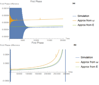
Figure 2: Graph of the phase difference between the first and second oscillator and its approximation for $\omega_{0}=1,\gamma=0.005,\epsilon=-0.1$ and initial condition given by the approximation to the damped and driven breathers of Section 2.2; (a) is graphed between times $0$ and $20\,000$, and (b) between times $0$ and $295\,000$, approximately when it leaves the metastable state.

Speaking colloquially, our numerics show that the metastable state slides along the family of damped and driven breathers. This is consistent with our computations of the spectrum of the linearization which showed that the span of the eigenspace of the zero eigenvector and the eigenvector with small positive eigenvalue was very close to the tangent plane of the family of damped and driven breathers. Moreover, this allows for the modeling of the dynamical evolution of the metastable state of the damped system from the damped and driven breathers (especially the time evolution of the phases) for long times. We believe that the period for which this approximation is accurate is connected to the bifurcations of the undamped system.

In Figure 3, we present numerics for a system with $N=8$ sites, which show that the effects we have described persist for systems with larger numbers of oscillators. Again we note that once the system has fully settled in the metastable state, we observe an initial, almost flat state where the system moves along the family of damped and driven breathers for a very long time. The system eventually reaches a point where the energy of the first oscillator decays suddenly while that of the other oscillators rise to meet it until they have the same energy, after which they reach the thermalized state and decay exponentially. The sudden decay in the energy is significantly more dramatic for the eight sites than it was for two or three sites.

Thus, we conjecture that the general evolution of these metastable states is as follows. When the trajectory is “captured” by one of the damped and driven breathers, the system begins to evolve by drifting along this family until the family of breathers disappears through bifurcation, at which point the system may be captured by another attractive family of approximately periodic orbits. There may, of course be other, possibly large, parts of the phase space where these metastable solutions do not exist and the evolution of the system is chaotic. In particular, it is not clear what properties of the periodic orbit in the undamped Hamiltonian system result in the solution becoming attractive once the system is subjected to damping.

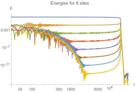
Figure 3: The energy of each oscillator in an eight-site system. The parameters chosen were $\gamma=0.05$, $\epsilon=-0.1$, and the initial condition is $p_{1}=1$ and all other $p_{j},q_{j}=0$.

We now turn to a discussion of the two-site damped and driven system where many of the phenomena discussed above can be illustrated by explicit computations. A detailed derivation is found in Appendix B, while in this section we will mostly show the results. The family of breathers of the Damped and Driven system related to the metastable state we have studied is analytically calculated to be:

$$E_{1}=\frac{1}{2}\sqrt{\frac{\gamma}{\beta}}\sqrt{\epsilon^{2}-\gamma\beta},\quad E_{2}=\frac{1}{2}\sqrt{\frac{\beta}{\gamma}}\sqrt{\epsilon^{2}-\gamma\beta},\quad\psi=\Bigg{\{}\begin{array}[]{cc}-\pi+\arcsin\left(\frac{\sqrt{\gamma\beta}}{\epsilon}\right)&\quad\epsilon>0\\ -\arcsin\left(\frac{\sqrt{\gamma\beta}}{\epsilon}\right)&\quad\epsilon<0.\end{array}$$ (78)

We can compute the spectrum of the linearization around these breathers, first writing out the Jacobian and then using Mathematica to derive series approximations. The small positive eigenvalue is:

$$\lambda_{2} = 4\gamma\left(\frac{\epsilon}{\omega}\right)^{2}+\mathcal{O}(\gamma\epsilon^{4})$$ (79)

The zero eigenvalue, $\lambda_{1}$, is absent in the energy-phase representation, because it corresponds to uniform phase rotation at all sites, and the energy-phase representation considers only phase differences between adjacent sites and hence is insensitive to phase rotations of the whole system. The leading order term in the small positive eigenvalue $\lambda_{2}$ has the same form as we derived in equation (43), if we set $N=2$ in that formula, as expected.

In Appendix B, we derive an approximation to the time evolution of the metastable state using the Ansatz that the solution maintains the relation $E_{1}(t)-E_{2}(t)=\sqrt{E(t)^{2}-\epsilon^{2}}$ resulting in an expression for the phase shift:

$$\sin\psi=\frac{\gamma}{2\sqrt{E^{2}-\epsilon^{2}}}$$ (80)

Note that this is only an approximation to the solution - this value of $\psi$ will not satisfy the equation for $\dot{\psi}$. However Figure 4 shows that it is a very accurate approximation when $E\gtrsim|\epsilon|$.

This result can then be used to calculate an approximation to the time evolution of the energy with initial energy $E(0)=E_{0}$:

$$E(t)\approx\frac{|\epsilon|}{2}\left(\sqrt{-W_{-1}\left(-e^{-1+4\gamma(t-\tau)}\right)}+\frac{1}{\sqrt{-W_{-1}\left(-e^{-1+4\gamma(t-\tau)}\right)}}\right)$$ (81)

Here $W_{-1}$ is the $-1$ branch of the product logarithm, and $\tau$ is the time for which $\lim_{t\to\tau}E(t)=|\epsilon|$ and is given by:

$$\tau=\frac{1}{2\gamma}\left(E_{0}\frac{E_{0}+\sqrt{E_{0}^{2}-\epsilon^{2}}}{\epsilon^{2}}-\ln\left(\frac{E_{0}+\sqrt{E_{0}^{2}-\epsilon^{2}}}{|\epsilon|}\right)-1\right)$$ (82)

If (81) was exact, $\tau$ would be the time when $E=|\epsilon|$, corresponding to the bifurcation for the undamped system, therefore the solution would be valid up until $\tau$. Since this is not the case, $\tau$ instead serves as an approximation for the time at which (81) stops working. In fact, the approximation stops working a small amount of time before $\tau$. This is expected since (80) does not make sense for $E>\sqrt{\epsilon^{2}-\tfrac{\gamma^{2}}{4}}$ due to the domain of the $\arcsin$.

Figure 4 shows the effectiveness of the approximation. $E_{0}$ was chosen so that it coincided with the initial energy of the graphs in the previous sections, leading to $\tau=4700.8$. The energy was graphed for longer than $\tau$ to identify the behaviour after it leaves the breather, while the phase difference was graphed for less than $\tau$ since the expression for the approximation explodes due to the singularity in the $\arcsin$. After this, the behavior of the solution is governed either by (102) or (103). Note that by approximating the energy of the solution by the expression for the energy of the breather in (105) we are assuming that this approximation moves along the family of breathers and from Figure 4 we again see that this scenario accurately reproduces the observed numerical behavior of the solution of the system.

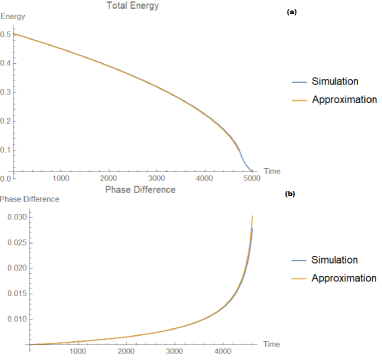
Figure 4: Graphs of the total energy and the phase difference for $E_{0}=0.505,\epsilon=-0.1,\gamma=0.005$. (a) Is the total energy graphed from $t=0$ to $t=\tau+300\approx 5000$ and (b) is the phase difference graphed from $t=0$ to $\tau-100\approx 4600$.

6 Summary and Conclusions

In this paper we have derived a new family of periodic solutions of the damped and driven discrete nonlinear Schrödinger equation. We have derived approximations to these solutions and analyzed their stability. We have also proposed an explanation for the appearance of very long-lived metastable states in the phase space of weakly damped lattice systems in which the trajectory is attracted to a cylinder of such breathers and then drifts very slowly along the cylinder of breathers until this family of solutions disappears. We suspect that the disappearance occurs near a bifurcation of the undamped system. Finally, we have shown that certain aspects of the metastable states are better approximated by these damped and driven breathers than by the breather solutions of the undamped lattice system.

Acknowledgements: The research of CEW was supported in part by NSF grant DMS-18133. CEW also acknowledges many helpful conversations about breather solutions in the dNLS equation with J.-P. Eckmann. DAC is thankful for the support from Boston University’s Undergraduate Research Opportunities Program.

Appendix A Proof of Theorem 2

In this appendix, we apply the implicit function theorem to establish the existence of the breather solutions discussed in Theorem 2. We begin by defining a function whose components are the equations for $\dot{p}_{j}$ and $\dot{q}_{j}$. Thus, we set

$$f_{j}(p_{2},p_{3},\dots,p_{N},q_{2},q_{3},\dots,q_{N};\epsilon,\omega,\gamma,p_{1},q_{1})=$$ (83)

$$\qquad\qquad\qquad\qquad=\epsilon(q_{j+1}+q_{j-1}-2q_{j})+\omega q_{j}-(p_{j}^{2}+q_{j}^{2})q_{j}$$

$$f_{j+N}(p_{2},p_{3},\dots,p_{N},q_{2},q_{3},\dots,q_{N};\epsilon,\omega,\gamma,p_{1},q_{1})=$$ (84)

$$\qquad\qquad\qquad\qquad=-\epsilon(p_{j+1}+p_{j-1}-2p_{j})-\omega p_{j}+(p_{j}^{2}+q_{j}^{2})p_{j}\ ,$$

for $j=2,3,\dots N-1$, and

$$f_{N}(p_{2},p_{3},\dots,p_{N},q_{2},q_{3},\dots,q_{N};\epsilon,\omega,\gamma,p_{1},q_{1})=$$ (85)

$$\qquad\qquad\qquad\qquad=\epsilon(q_{N-1}-q_{N})+\omega q_{N}-(p_{N}^{2}+q_{N}^{2})q_{N}-\gamma p_{N}$$

$$f_{2N}(p_{2},p_{3},\dots,p_{N},q_{2},q_{3},\dots,q_{N};\epsilon,\omega,\gamma,p_{1},q_{1})=$$ (86)

$$\qquad\qquad\qquad\qquad=-\epsilon(p_{N-1}-p_{N})-\omega p_{N}+(p_{N}^{2}+q_{N}^{2})p_{N}-\gamma q_{N}.$$

Defining

$$F(p_{2},p_{3},\dots,p_{N},q_{2},q_{3},\dots,q_{N};\epsilon,\omega,\gamma,p_{1},q_{1})=$$

$$\qquad\qquad=(f_{2},f_{3},\dots,f_{N},f_{N+2},f_{N+3},\dots,f_{2N})\ ,$$ (87)

we see that $F:{\mathbb{R}}^{2(N-1)}\times{\mathbb{R}}^{5}\to{\mathbb{R}}^{2(N-1)}$ and that $F(0,0,\dots,0;0,1,0,1,0)=0$. Computing the Jacobian at this fixed point gives:

$$D_{(\tilde{p},\tilde{q})}F=\left(\begin{array}[]{cc}0&1\\ -1&0\end{array}\right)$$ (88)

where $\tilde{p}=(p_{2},\dots,p_{N})$, $\tilde{q}=(q_{2},\dots,q_{N})$, and where $0$ represents and $(N-1)\times(N-1)$ matrix of zeros and $1$ represents an $(N-1)\times(N-1)$ dimensional identity matrix.

Thus, by the Implicit Function Theorem, for every $\epsilon,\gamma,q_{1}$ sufficiently close to zero and every $\omega$ and $p_{1}$ sufficiently close to $1$, there exists (a unique) $p_{2}^{*},\dots,p_{N}^{*},q_{2}^{*},\dots,q_{N}^{*}$ such that

$$F(p_{2}^{*},p_{3}^{*},\dots,p_{N}^{*},q_{2}^{*},q_{3}^{*},\dots,q_{N}^{*};\epsilon,\omega,\gamma,p_{1},q_{1})=0\ .$$ (89)

Furthermore, the solution $(p_{2}^{*},\dots,p_{N}^{*},q_{2}^{*},\dots,q_{N}^{*})$ depends smoothly (in fact, analytically) on $(\epsilon,\omega,\gamma,p_{1},q_{1})$.

Finally, consider the two equations for $\dot{p}_{1}$ and $\dot{q}_{1}$. In order to have a fixed point, we need

$$f_{1}(\epsilon,\omega,\beta,p_{1},q_{1},p_{2},q_{2})=$$ (90)

$$\qquad=\epsilon(q_{2}-q_{1})+\omega q_{1}-(q_{1}^{2}+p_{1}^{2})q_{1}+\beta p_{1}=0$$

$$f_{N+1}(\epsilon,\omega,\beta,p_{1},q_{1},p_{2},q_{2})=$$ (91)

$$\qquad=-\epsilon(p_{2}-p_{1})-\omega p_{1}+(q_{1}^{2}+p_{1}^{2})p_{1}+\beta q_{1}=0$$

By rotational invariance, we choose $q_{1}=0$. Then, inserting the solutions $q_{2}^{*}$ and $p_{2}^{*}$ from above, from the requirement that $f_{1}=0$, we see that we must have

$$\beta p_{1}=-\epsilon q_{2}^{*}\ ,$$ (92)

while the requirement that $f_{N+1}=0$ implies

$$-\epsilon(p_{2}^{*}-p_{1})-\omega p_{1}+p_{1}^{3}=0\ .$$ (93)

Using the implicit function theorem, and the fact that $p_{2}^{*}$ depends smoothly on $p_{1}$, we see that there exists a solution $p_{1}^{*}$ of (93), for $\omega$ near $1$ and $\gamma$ and $\epsilon$ sufficiently small which satisfies $(p_{1}^{*})^{2}=\omega+{\cal{O}}(\epsilon)$. Inserting this into (92), we see that there is a unique value of $\beta$ (depending smoothly on $\epsilon$, $\gamma$, and $\omega$), such that we have a damped and driven breather near the $(1,0,0,\dots,0)$ breather, for each value of $\omega$ near one and $\epsilon$ and $\gamma$ sufficiently small.

Appendix B Detailed analysis of the two site system

The simplicity of the two-site system allows for a more global investigation of the phase space. Once again, the analysis is better suited to using the energy-phase equations rather than expressing the system in the $p,q$ coordinates, and the energy-phase equations for the two-site system give the simple system of three ODEs:

$$\dot{E}_{1} = 2\epsilon\sqrt{E_{1}E_{2}}\sin\psi+2\beta E_{1}$$ (94)

$$\dot{E}_{2} = -2\epsilon\sqrt{E_{1}E_{2}}\sin\psi-2\gamma E_{2}$$

$$\dot{\psi} = 2(E_{2}-E_{1})\left(1+\epsilon\frac{\cos\psi}{2\sqrt{E_{1}E_{2}}}\right)$$

For the undriven-undamped, two-site system, (i.e. $\gamma=\beta=0$), all breather solutions were found in [32] and in our notation they take the form:

$$E_{1}^{(1)}=\tfrac{1}{2}E\quad E_{2}^{(1)}=\tfrac{1}{2}E \quad\psi^{(1)}=0$$ (95)

$$E_{1}^{(2)}=\tfrac{1}{2}E\quad E_{2}^{(2)}=\tfrac{1}{2}E \quad\psi^{(2)}=\pi$$ (96)

$$E_{1}^{(3)}=\tfrac{1}{2}\left(E+\sqrt{E^{2}-\epsilon^{2}}\right)\quad E_{2}^{(3)}=\tfrac{1}{2}\left(E-\sqrt{E^{2}-\epsilon^{2}}\right) \quad\psi^{(3)}=\pi$$ (97)

$$E_{1}^{(4)}=\tfrac{1}{2}\left(E-\sqrt{E^{2}-\epsilon^{2}}\right)\quad E_{2}^{(4)}=\tfrac{1}{2}\left(E+\sqrt{E^{2}-\epsilon^{2}}\right) \quad\psi^{(4)}=\pi$$ (98)

when $\epsilon>0$ with similar expressions for $\epsilon<0$. For each of these breathers, we can calculate the angular frequency $\omega$ from $E$. The values are $\omega^{(1)}=E,\omega^{(2)}=E+2\epsilon,\omega^{(3)}=\omega^{(4)}=2E+\epsilon$. The third breather is the one close to the metastable states discussed so far.

These breathers continue to the damped and driven setting , and again, one can derive explicit formulas for them by calculating the fixed points of (94) - for example, if $0<\beta<<\gamma$, and $\beta\gamma<\epsilon^{2}$, the family of breathers $E^{(3)}$, continues to a family of the form described by (78) (Note that to compare these formulas with those derived for the general $N$-site damped and driven breather, one should first fix $\gamma$ and $\epsilon$ and then choose $\beta$ so that $E^{(3)}_{1}=1/2$, since those breathers were chosen to be close to the breather with $p_{1}=1$ and all other components zero.)

If we linearize energy-phase system system (94) about this breather, the Jacobian matrix takes the form:

$$\left(\begin{array}[]{ccc}\beta&-\gamma&-(\varepsilon^{2}-\gamma\beta)\\ \beta&-\gamma&(\varepsilon^{2}-\gamma\beta)\\ -1+\frac{\beta}{\gamma}&1-\frac{\gamma}{\beta}&\beta-\gamma\end{array}\right)$$ (99)

Using Mathematica to derive series approximations for the solutions of the characteristic polynomial, we find the eigenvalues of the linearization are the eigenvalue $\lambda_{2}$, given by (79) and:

$$\lambda_{3} = -\gamma\left(1+\left(\frac{\epsilon}{\omega}\right)^{2}+\mathcal{O}(\epsilon^{4})\right)+i\left(\omega+\mathcal{O}(\epsilon^{2})\right)$$ (100)

$$\lambda_{4} = -\gamma\left(1+\left(\frac{\epsilon}{\omega}\right)^{2}+\mathcal{O}(\epsilon^{4})\right)-i\left(\omega+\mathcal{O}(\epsilon^{2})\right)$$ (101)

These two eigenvalues are close to $\pm i\omega$, but with strictly negative real part, proportional to $\gamma$, as expected. An important fact to notice is that if we instead find the linearization about this fixed point using the $p,q$ coordinates, we obtain the same eigenvalues $\lambda_{2},\lambda_{3},\lambda_{4}$, with an added $0$ eigenvalue corresponding to the invariance with respect to rotations about the cylinder of breathers.

For $|\epsilon|>>\gamma>0$ but $\beta=0$, the breathers disappear but they can be used to help find approximate solutions of the damped problem, and to understand its metastable behavior. For example, if we make the Ansatz that $E_{1}(t)=E_{2}(t)$ for all time, and substitute this into the equations of motion we find exact solutions:

$$E_{1}(t)=\tfrac{1}{2}E_{0}e^{-\gamma t}\quad E_{2}(t)=\tfrac{1}{2}E_{0}e^{-\gamma t} \quad\psi(t)=\ -\arcsin\left(\frac{\gamma}{2\epsilon}\right)$$ (102)

$$E_{1}(t)=\tfrac{1}{2}E_{0}e^{-\gamma t}\quad E_{2}(t)=\tfrac{1}{2}E_{0}e^{-\gamma t} \quad\psi(t)=-\pi+\arcsin\left(\frac{\gamma}{2\epsilon}\right)$$ (103)

where $E_{0}=E_{1}(0)+E_{2}(0)$ is the initial total energy, and $\epsilon>0$. One has similar expressions when $\epsilon<0$. These are the states corresponding to (95) and (96) respectively, with only the first of these being stable.

We can use a similar argument to approximate the effects of initial conditions close to the solution $E^{(3)}$ of (95). First, differentiate $\tfrac{d}{dt}E_{1}^{(3)}$ and $\tfrac{d}{dt}E_{2}^{(3)}$:

$$\frac{d}{dt}E_{1}^{(3)} = \frac{1}{2}\dot{E}\left(1+\frac{E}{\sqrt{E^{2}-\epsilon^{2}}}\right)$$

$$\frac{d}{dt}E_{2}^{(3)} = \frac{1}{2}\dot{E}\left(1-\frac{E}{\sqrt{E^{2}-\epsilon^{2}}}\right)$$

Using $\dot{E}=\dot{E}_{1}+\dot{E_{2}}=-2\gamma E_{2}$, and considering $E_{1}=E_{1}^{(3)},E_{2}=E_{2}^{(3)}$, we set:

$$\tfrac{d}{dt}E_{1}^{(3)}-\tfrac{d}{dt}E_{2}^{(3)}=\dot{E}_{1}-\dot{E}_{2}=-2\epsilon\sqrt{E_{1}E_{2}}\sin\psi-(2\epsilon\sqrt{E_{1}E_{2}}-2\gamma E_{2})$$ (104)

Solving for $\sin\psi$ we get (80). However, if we calculate $\dot{\psi}$ from this expression, it will not match the expression in the equations of motion, meaning that the solution is not exact. This is expected due to the metastability of the state, the solution cannot be described by these equations for all time. Numerically, the above expression provides a very good approximation for long time. Recall that for this breather $\omega^{(3)}=2E+\epsilon$, so calculating the leading order in $\psi$ we find $\psi=\tfrac{\gamma}{\omega}+\dots$, which is identical to the value of the twist in the damped and driven breather from Theorem 3. This is further evidence of the fact that the damped and driven breathers provide a better approximation to the metastable states than do the undamped breathers.

We also obtain an approximation to the time evolution of the energy through:

$$\dot{E}=-2\gamma E_{2}\approx-2\gamma E_{2}^{(3)}=-\gamma\left(E-\sqrt{E^{2}-\epsilon^{2}}\right)$$ (105)

If the system starts with initial total energy $E_{0}$, an approximate expression we simply solve the integral:

$$\int_{E_{0}}^{E(t)}\frac{dx}{x-\sqrt{x^{2}-\epsilon^{2}}}=-\gamma t$$ (106)

If we set the upper limit to be $\epsilon$ and the right hand side to be $-\gamma\tau$, we obtain (82), using the indefinite integral:

$$\int\frac{dx}{x-\sqrt{x^{2}-\epsilon^{2}}}=\frac{1}{2}\left[x\frac{x+\sqrt{x^{2}-\epsilon^{2}}}{\epsilon^{2}}-\ln\left(x+\sqrt{x^{2}-\epsilon^{2}}\right)\right]$$ (107)

To obtain (81), it is worth defining:

$$f(t)=E(t)+\sqrt{E(t)^{2}-\epsilon^{2}}$$ (108)

Then, evaluating the indefinite integral (107) at $E(t),E_{0}$, will lead to an algebraic equation in $f(t)$:

$$4\gamma t-2\frac{E_{0}}{\epsilon^{2}}+1=-\left(\frac{f(t)}{\epsilon}\right)^{2}+\ln\left(\left(\frac{f(t)}{f(0)}\right)^{2}\right)$$ (109)

Which can be shown to solve to:

$$f(t)=\epsilon\sqrt{-W_{-1}(e^{-1+4\gamma(t-\tau)})}$$ (110)

From where (81) is derived, and $\tau$ defined as in (82). To get that the branch of the product logarithm, we take the limit:

$$\lim_{t\to 0}E(t)=E_{0}$$ (111)

References

- [1] Jean-Pierre Eckmann, Claude-Alain Pillet, and Luc Rey-Bellet. Entropy production in nonlinear, thermally driven Hamiltonian systems. J. Statist. Phys., 95(1-2):305–331, 1999.
- [2] Stefano Iubini, Stefano Lepri, Roberto Livi, Antonio Politi, and Paolo Politi. Nonequilibrium Phenomena in Nonlinear Lattices: From Slow Relaxation to Anomalous Transport, pages 185–203. Springer International Publishing, 2020.
- [3] C. Danieli, D. K. Campbell, and S. Flach. Intermittent many-body dynamics at equilibrium. Phys. Rev. E, 95:060202, June 2017.
- [4] Carlo Danieli, Thudiyangal Mithun, Yagmur Kati, David K. Campbell, and Sergej Flach. Dynamical glass in weakly nonintegrable Klein-Gordon chains. Phys. Rev. E, 100:032217, Sep 2019.
- [5] Martin Hairer and Jonathan C. Mattingly. Slow energy dissipation in anharmonic oscillator chains. Communications on Pure and Applied Mathematics, 62(8):999–1032, 2009.
- [6] Salvatore D. Pace and David K. Campbell. Behavior and breakdown of higher-order Fermi-Pasta-Ulam-Tsingou recurrences. Chaos: An Interdisciplinary Journal of Nonlinear Science, 29(2):023132, 2019.
- [7] K. Ø. Rasmussen, T. Cretegny, P. G. Kevrekidis, and Niels Grønbech-Jensen. Statistical mechanics of a discrete nonlinear system. Phys. Rev. Lett., 84:3740–3743, Apr 2000.
- [8] Uri Levy and Yaron Silberberg. Equilibrium temperatures of discrete nonlinear systems. Phys. Rev. B, 98:060303, Aug 2018.
- [9] J.-P. Eckmann and C.E. Wayne. Breathers as metastable states for the discrete NLS equation. Discrete & Continuous Dynamical Systems - A, 38:6091–6103, 2018.
- [10] Sergej Flach and Andrey V. Gorbach. Discrete breathers — advances in theory and applications. Physics Reports, 467(1):1 – 116, 2008.
- [11] J.-P. Eckmann and C.E. Wayne. Decay of hamiltonian breathers under dissiptation. Comm. Math. Phys., 380:71–102, 2020.
- [12] Holger Hennig and Ragnar Fleischmann. Nature of self-localization of Bose-Einstein condensates in optical lattices. Physical Review A, 87:033605, 2013.
- [13] Roberto Livi, Roberto Franzosi, and Gian-Luca Oppo. Self-localization of Bose-Einstein condensates in optical lattices via boundary dissipation. Phys. Rev. Lett., 97:060401, Aug 2006.
- [14] N. Cuneo, J.-P. Eckmann, and C. Poquet. Non-equilibrium steady state and subgeometric ergodicity for a chain of three coupled rotors. Nonlinearity, 28(7):2397–2421, jun 2015.
- [15] U. Peschel, O. Egorov, and F. Lederer. Discrete cavity solitons. Opt. Lett., 29(16):1909–1911, Aug 2004.
- [16] Jaroslaw E. Prilepsky, Alexey V. Yulin, Magnus Johansson, and Stanislav A. Derevyanko. Discrete solitons in coupled active lasing cavities. Opt. Lett., 37(22):4600–4602, Nov 2012.
- [17] Nikolaos K. Efremidis and Demetrios N. Christodoulides. Discrete Ginzburg-Landau solitons. Phys. Rev. E, 67:026606, Feb 2003.
- [18] Dirk Hennig. Periodic, quasiperiodic, and chaotic localized solutions of a driven, damped nonlinear lattice. Phys. Rev. E, 59:1637–1645, Feb 1999.
- [19] J. L. Marín, F. Falo, P. J. Martínez, and L. M. Floría. Discrete breathers in dissipative lattices. Phys. Rev. E, 63:066603, May 2001.
- [20] Jacques-Alexandre Sepulchre and Robert S MacKay. Localized oscillations in conservative or dissipative networks of weakly coupled autonomous oscillators. Nonlinearity, 10(3):679–713, may 1997.
- [21] Ramaz Khomeriki. Nonlinear band gap transmission in optical waveguide arrays. Phys. Rev. Lett., 92:063905, Feb 2004.
- [22] P. Maniadis, G. Kopidakis, and S. Aubry. Energy dissipation threshold and self-induced transparency in systems with discrete breathers. Physica D: Nonlinear Phenomena, 216(1):121–135, 2006. Nonlinear Physics: Condensed Matter, Dynamical Systems and Biophysics.
- [23] Vladimir V. Konotop, Jianke Yang, and Dmitry A. Zezyulin. Nonlinear waves in -symmetric systems. Rev. Mod. Phys., 88:035002, Jul 2016.
- [24] L. Jin and Z. Song. Solutions of -symmetric tight-binding chain and its equivalent hermitian counterpart. Phys. Rev. A, 80:052107, Nov 2009.
- [25] Yogesh N. Joglekar, Derek Scott, Mark Babbey, and Avadh Saxena. Robust and fragile -symmetric phases in a tight-binding chain. Phys. Rev. A, 82:030103, Sep 2010.
- [26] G. Theocharis, M. Kavousanakis, P. G. Kevrekidis, Chiara Daraio, Mason A. Porter, and I. G. Kevrekidis. Localized breathing modes in granular crystals with defects. Phys. Rev. E, 80:066601, Dec 2009.
- [27] Panayotis Panayotaros and Felipe Rivero. Multi-peak breather stability in a dissipative discrete Nonlinear Schrödinger (NLS) equation. Journal of Nonlinear Optical Physics & Materials, 23(04):1450044, 2014.
- [28] R. S. MacKay and S. Aubry. Proof of existence of breathers for time-reversible or Hamiltonian networks of weakly coupled oscillators. Nonlinearity, 7(6):1623–1643, nov 1994.
- [29] S. Flach and C. R. Willis. Discrete breathers. Phys. Rep., 295(5):181–264, 1998.
- [30] P. G. Kevrekidis, K. Ø. Rasmussen, and A. R. Bishop. The discrete nonlinear Schrödinger equation: A survey of recent results. International Journal of Modern Physics B, 15(21):2833–2900, 2001.
- [31] Noé Cuneo, Jean-Pierre Eckmann, and C. Eugene Wayne. Energy dissipation in hamiltonian chains of rotators. Nonlinearity, 30(11):R81–R117, oct 2017.
- [32] J.C. Eilbeck, P.S. Lomdahl, and A.C. Scott. The discrete self-trapping equation. Physica D: Nonlinear Phenomena, 16(3):318 – 338, 1985.