Abstract

Phase I clinical trials are designed to test the safety (non-toxicity) of drugs and find the maximum tolerated dose (MTD). This task becomes significantly more challenging when multiple-drug dose-combinations (DC) are involved, due to the inherent conflict between the exponentially increasing DC candidates and the limited patient budget. This paper proposes a novel Bayesian design, SDF-Bayes, for finding the MTD for drug combinations in the presence of safety constraints. Rather than the conventional principle of escalating or de-escalating the current dose of one drug (perhaps alternating between drugs), SDF-Bayes proceeds by cautious optimism: it chooses the next DC that, on the basis of current information, is most likely to be the MTD (optimism), subject to the constraint that it only chooses DCs that have a high probability of being safe (caution). We also propose an extension, SDF-Bayes-AR, that accounts for patient heterogeneity and enables heterogeneous patient recruitment. Extensive experiments based on both synthetic and real-world datasets demonstrate the advantages of SDF-Bayes over state of the art DC trial designs in terms of accuracy and safety.

1 INTRODUCTION

The use of combinations of drugs is becoming an increasingly valuable–and common–treatment modality (Bamias et al.,, 2011; Flaherty et al.,, 2012; Ocana et al.,, 2019; Kelly and Halabi,, 2018), especially in the treatment of cancer, where it has been widely observed that combinations of drugs can be effective when single drugs are not (Paller et al.,, 2019). (Similar observations have been made for other diseases, including COVID-19.) As a result, there has been an enormous effort to test and validate drug combinations for treatment; indeed combination trials now account for more than 25% of all clinical trials in oncology (Wu et al.,, 2014).

However, clinical trials of drug combinations face greater challenges than those of single drugs, especially in Phase I trials which are required to find safe doses. The essential problem is that the number of potential dose-combinations (DCs) to be tested in a trial increases exponentially with the number of drugs, but the patient budget cannot scale proportionately. Indeed, a typical real-world Phase I trial often recruits fewer than 100 patients; a few examples are shown in Table 1. The limited patient budget constrains the number of DCs that can be throughly tested. Moreover, because drugs interact differently with different body chemistry of different groups of patients (e.g., with the different hormone balances and levels in males and females), it is frequently possible to identify in advance groups of patients who might be expected to exhibit very different tolerances for the same DC (Sun and Braun,, 2015; Kim et al.,, 2009; Dasari et al.,, 2013; Moss et al.,, 2015; Wages et al.,, 2015).

In view of the growing importance of drug combinations in the treatment of disease, it is of enormous importance to design Phase I drug combination trials in a way that is efficient, informative and safe (Hamberg et al.,, 2010). This design includes the path of DC testing and, in the presence of identified heterogeneous groups, the allocation of patient budgets to groups as well.

Table 1: Examples of Phase I clinical trial studies with drug combinations

Study	Drugs	No. of DC	No. of Patients	Target disease
(Plummer et al.,, 2008)	Rucaparib & temozolomide	12	32	Advanced solid tumors
(Bailey et al.,, 2009)	Nilotinib & imatinib	20	50	Gastrointestinal stromal tumors
(Bagatell et al.,, 2014)	Temsirolimus & irinotecan & temozolomide	24	71	Solid tumors
(Calvo et al.,, 2017)	Dacomitinib & Figitumumab	12	74	Advanced solid tumors

This paper develops a new dose-finding Phase I clinical trial method for drug combinations and heterogeneous patient groups and demonstrates that it is superior to existing methods. For a given patient budget, the design objective is to maximize the probability of finding the maximum tolerated dose (MTD), defined to be the DC that is closest to a given target toxicity threshold, subject to constraints on the exposure of patients to unsafe doses throughout the trial. Our safe dose-finding (SDF) method employs an adaptive design: the DC to be tested in the current round is chosen on the basis of past observations. This is possible because Phase I trials are not blind; the trialist knows the DC given to each patient and observes the outcome. The SDF-Bayes algorithm builds on a novel learning principle we call Cautious Optimism, which manifests by combining two opposing ideas: (1) SDF-Bayes constrains the choice of DC to be tested in the current round to a set of DCs that it estimates to be unlikely to violate the safety constraint; this is the principle of caution, and (2) within this constrained set of DCs, SDF-Bayes chooses the DC to be tested in the current round to be the one estimated to be most likely to be the MTD; this is the optimistic belief principle (Aziz et al.,, 2019).

To deal with settings in which potentially heterogeneous patient groups can be identified in advance, we also propose a extension, that we call SDF-Bayes-AR, in which both the DC to be tested and the patient group to be sampled in the current round are chosen adaptively. To determine the group from which to recruit the next patient, SDF-Bayes-AR uses the criterion of expected improvement (EI). Adaptive recruitment is especially useful when there is prior information about one or several groups (Pallmann et al.,, 2018; Park et al.,, 2018; Atan et al.,, 2019), and an appealing feature of our approach is that it can smoothly incorporate prior information, be it from the drug development phase, from dose-toxicity models, from tests in vitro and in animals, or from previous trials (Gasparini,, 2013; Shen et al.,, 2019).

We validate the proposed designs via extensive simulated trials using both synthetic and real-world datasets. We show that, using a realistic number of patients, our algorithms provide significantly more accurate recommendations than state-of-the-art designs, while obeying the safety constraints, for both homogeneous and heterogeneous patient populations.

2 DC-FINDING CLINICAL TRIALS

2.1 Dose-Toxicity Model

We consider a dual-agent dose-finding Phase I clinical trial for the combination of agents (drugs) A and B. We assume discrete dose levels $\mathcal{J}\!=\!\{1,...,J\}$ for agent A and $\mathcal{K}\!=\!\{1,...,K\}$ for agent B. We use $(j,k)$ to denote the combination of dose $j$ of agent A and dose $k$ of agent B so that the set of all DCs is just $\mathcal{A}\!=\!\mathcal{J}\times\mathcal{K}$. We model the toxicity event $Y_{jk}$ of DC $(j,k)$ as a Bernoulli random variable with unknown parameter $p_{jk}$. We set $Y_{jk}=1$ to indicate that a dose-limiting toxicity (DLT) was observed for $(j,k)$, and $Y_{jk}=0$ otherwise.

We assume the toxicities follow a parametric joint dose-toxicity model

$$\pi:\Theta\times\mathcal{J}\times\mathcal{K}\to[0,1]\vspace{-3pt}$$ (1)

where $\Theta$ is some space of parameters, and $\pi(\theta,j,k)=p_{jk}(\theta)$ is the toxicity of the DC $(j,k)$ if the parameter is $\theta\in\Theta$. The true vector of parameters $\theta^{*}$ is unknown and must be learned/estimated. The literature has suggested various dose-toxicity models (Gasparini,, 2013; Riviere et al.,, 2014); we present details of some commonly-used models in the Supplementary Material; we focus here on developing a methodology that can be used with many parametric joint dose-toxicity models.

2.2 Problem Formulation

We consider an adaptive Phase I clinical trial for drug combinations with a given patient budget $T$. The nominal trial objective is to find the DC whose estimated toxicity is closest to the threshold $\xi$; i.e. to find any DC that belongs to

$$\mathcal{A}^{*}=\mathop{\rm argmin}_{jk}\big{|}p_{jk}(\theta^{*})-\xi\big{|}.\vspace{-6pt}$$

For each $t$, write $\mathcal{O}(t)=\{(Y_{\tau},a(\tau))\}^{t-1}_{\tau=1}$ for the history of trial actions and observations before $t$; $a(\tau)$ is the DC that was administered to patient $\tau$ and $Y_{\tau}$ is the observed toxicity for DC $a(\tau)$ on patient $\tau$. As in typical adaptive clinical trial designs, all DCs are actionable in the trial. A DC-finding algorithm $\Pi$ maps the history $\mathcal{O}(t)$ to the DC $a(t)\in\mathcal{A}$ that is to be administered to patient $t$. At the end of the clinical trial, the algorithm recommends a DC $\hat{a}^{*}$. The recommendation is correct if $\hat{a}^{*}\in\mathcal{A}^{*}$; otherwise the recommendation is an error. We set the objective of our algorithm to minimize the probability that errors occur. (Because the occurrence of toxicity events is stochastic, there is always some positive probability that errors will occur.)

Because testing unsafe DCs should be avoided, we insist that, with high probability, the average toxicity should not exceed the toxicity threshold plus a margin of error. We formalize this by defining the DLT observation rate to be

$$S(T)=\frac{1}{T}\sum_{t=1}^{T}Y_{t}\vspace{-3pt}$$

and we impose the safety constraint

$$\mathbb{P}\big{(}S(T)\leq\xi+\epsilon\big{)}\geq 1-\delta,\vspace{-3pt}$$ (2)

where $\epsilon>0$ is a prescribed margin of error and $\delta>0$ is a prescribed acceptable probability of failure.

3 CAUTIOUS OPTIMISM

3.1 Preliminaries

Given the dose-toxicity structure, we begin with a prior distribution $f(\theta)$ on the parameter vector $\theta$ and update the posterior distribution, based on the observations. (The assumption of a prior distribution is common in the literature, and is natural, because the toxicities of the individual drugs are usually understood on the basis of prior use, and the various drug combinations will have already been tested in vitro and in animals.) We write $f(\theta|\mathcal{O}(t))$ to denote the posterior distribution of $\theta$ following the history $\mathcal{O}(t)$. The likelihood of $\theta$ in round $t$ for the observations $\mathcal{O}(t)$ satisfies

$$L(\theta|\mathcal{O}(t))\propto\prod_{a\in\mathcal{A}}p_{a}(\theta)^{s_{a}(t)}(1-p_{a}(\theta))^{n_{a}(t)-s_{a}(t)},\vspace{-3pt}$$

where $n_{a}(t)$ is the number of times DC $a$ has been chosen before round $t$ and $s_{a}(t)=\sum_{\tau=1}^{t-1}\mathbb{I}[a(\tau)=a]Y_{\tau}$ is the number of DLTs observed for the DC $a$ before round $t$. The posterior distribution satisfies

$$f(\theta|\mathcal{O}(t))\propto L(\theta|\mathcal{O}(t))f(\theta).\vspace{-3pt}$$ (3)

3.2 Cautious Optimism in Bayesian SDF

We base our algorithm on the principle of “optimism in the face of uncertainty” (Bubeck and Cesa-Bianchi,, 2012), which means choosing the DC that is currently estimated to be most likely to be the MTD, but we maintain safety by constraining the set of DCs from which we choose.

Optimism for Efficiency

We assess which DC is most likely to be the MTD by using the posterior distribution $f(\theta|\mathcal{O})$ as described in (3). For this, in our algorithm we follow the literature (see (Riviere et al.,, 2014), for example) and find the DC

$$\mathop{\rm argmax}_{a}{\mathbb{P}}\big{(}\{\theta:|p_{a}(\theta)-\xi|<u\}\big{)},\vspace{-3pt}$$

where $u$ is some prescribed allowable margin of error, and the probability is taken with respect to the posterior distribution on the parameter space $\Theta$.

The probability $G_{a}^{\mathcal{O}(t)}(u)$ that the toxicity of DC $a$ belongs to the given target toxicity interval $[\xi-u,\xi+u]$ isrl G_a^O(t)(u)  &= P[p_a(θ)∈[ξ-u,ξ+u]—O(t)]
= ∫_ΘI[p_a(θ)∈[ξ-u,ξ+u]]f(θ—O(t))dθ. Then, we find a DC $a(t)$ that is deemed most likely to have toxicity in $[\xi-u,\xi+u]$; i.e.

$$a_{o}(t)=\mathop{\rm argmax}_{a}G_{a}^{\mathcal{O}(t)}(u).$$

The DC is chosen to be allocated if it is deemed “safe enough” (see the next paragraph) at round $t$. If the argmax is not a singleton, we choose arbitrarily, subject to maximizing the total dose of both drugs.

Caution for Safety

To determine the set of DCs that are “safe enough” in round $t$ we first choose a hyperparameter $v>0$ that controls conservativeness and define

$$F_{a}^{\mathcal{O}(\tau)}(v) =\max\Big{\{}x\in[0,1]:\mathbb{P}\big{[}p_{a}(\theta)\leq x\,\big{|}\,\mathcal{O}(\tau)\big{]}\leq v\Big{\}}$$

$$\Phi(t,v) =\sum_{\tau=1}^{t-1}F_{a(\tau)}^{\mathcal{O}(t)}(v)$$

$$r(t,v) =(\xi+\epsilon)t-\Phi(t,v).$$ (4)

Roughly speaking, $\Phi(t,v)$ represents the number of DLT observations that would have been expected before round $t$, given the posterior. For safety, we are “allowed” a DLT observation rate $\xi+\epsilon$ so if $\Phi(t,v)\leq(t-1)(\xi+\epsilon)$ the safety constraint holds in expectation after $t-1$ rounds; if we choose $a(t)$ so that $\Phi(t+1,v)\leq t(\xi+\epsilon)$ then we will have met the safety constraint in expectation after $t$ rounds. We cannot be assured of choosing such an $a(t)$ because we do not know what the posterior will be after $t$ rounds, but if the posterior after $t$ rounds were the same as the posterior after $t-1$ rounds and we choose $a(t)$ to have expected toxicity less than the residual $r(t,v)$ then the safety constraint will be met in expectation after $t$ rounds. So define

$$\mathcal{A}_{r}(t)\coloneqq\{a\in\mathcal{A}:F_{a}^{\mathcal{O}(t)}(v)\leq r(t,v)\}.\vspace{-3pt}$$ (5)

Unfortunately it might be that $a_{o}(t)\notin\mathcal{A}_{r}(t)$. (That would certainly be the case if $r(t,v)<0$, which means that the safety constraint had already been violated in expectation.) In that case we can use a conservative DC, one whose expected toxicity is no greater than $\xi$, so that after $t$ rounds the residual $r(t+1,v)$ will be greater than the residual $r(t,v)$. The set of conservative DCs is

$$\mathcal{A}_{c}(t)\coloneqq\{a\in\mathcal{A}:F_{a}^{\mathcal{O}(t)}(v)\leq\xi\}.\vspace{-3pt}$$

We allocate the most likely conservative DC to be the MTD; i.e., $\mathop{\rm argmax}_{a\in\mathcal{A}_{c}(t)}G_{a}^{\mathcal{O}(t)}(u)$. Finally, if $\mathcal{A}_{c}(t)=\emptyset$ we terminate the procedure with no recommendation.

Theoretical Guarantee

The following Proposition shows that, when this cautiously optimistic procedure can be carried out, it maintains the safety constraint by keeping the residual non-negative with a high probability. (The proof is in the Supplementary Materials.)

Proposition 1

Fix $t\leq T$. For each $\tau\leq t$, set $v_{\tau}=(1-\delta)^{1/\tau}$. If the residuals $r(\tau,v_{\tau})$ are non-negative for all $\tau\leq t$ then the cautious optimism principle in Bayesian SDF satisfies

$$\mathbb{P}\left[\left.\frac{1}{t}\sum_{\tau=1}^{t}p_{a(\tau)}(\theta)\leq\xi+\epsilon\right|\mathcal{O}(t)\right]\geq 1-\delta.$$

3.3 Algorithm Description

Here we provide an implementation of the cautious optimism principle described above. Because we are considering an arbitrary joint dose-toxicity model, our implementation relies on Bayesian sampling in order to ensure the universal applicability of the algorithm. We comment that our algorithm can be easily extended for drug combinations with more than two drugs if a corresponding dose-toxicity model is given.

We denote the number of samples from the posterior distribution $f(\theta|\mathcal{O})$ by $L$, and the samples in round $t$ as $\tilde{\Theta}(t)=\{\theta^{(l)}(t)\}_{l\in[L]}$. We use a Gibbs sampler (Gilks et al.,, 1995); this is a common multidimensional Bayesian sampling algorithm. Inside the Gibbs sampler, we use the adaptive rejection Metropolis sampling method (Gilks et al.,, 1995). Details can be found in the Supplementary Material.

In round $t$, we use the samples to approximate the probability $G_{a}^{\mathcal{O}(t)}(u)$ by

$$\tilde{G}_{a}^{\mathcal{O}(t)}(u)=\frac{1}{L}\sum_{l=1}^{L}\mathbb{I}\big{\{}t:\xi-u\leq p_{a}(\theta^{(l)}(t))\leq\xi+u\big{\}}.\vspace{-5pt}$$

Using this approximation, the DC most likely to be the MTD in round $t$ is $\tilde{a}_{o}(t)=\mathop{\rm argmax}_{a\in\mathcal{A}}\tilde{G}_{a}^{\mathcal{O}(t)}(u)$. SDF-Bayes then infers whether the safety constraint is violated or not for the chosen DC by evaluating the residual. To calculate the residual in practice, we define $\tilde{F}_{a}^{\mathcal{O}(t)}(v)\coloneqq\texttt{Prctile}(a,\tilde{\Theta}(t),v)$ that returns the percentile of the toxicities of DC $a$ calculated from the samples $\tilde{\Theta}(t)$ for the percentage $v\in[0,1]$. Then, from (4), we calculate the residual $r(t,v)$ in round $t$ by $r(t,v)=(\xi+\epsilon)t-\sum_{\tau=1}^{t-1}\tilde{F}_{a(\tau)}^{\mathcal{O}(t)}(v)$ and define $\tilde{\mathcal{A}}_{r}(t)$ as in (5) with $\tilde{F}_{a}^{\mathcal{O}(t)}(v)$. To keep the residual non-negative, SDF-Bayes accepts the chosen DC $\bar{a}(t)$ if it does not make the residual negative: $\tilde{a}_{o}(t)\in\tilde{\mathcal{A}}_{r}(t)$. Otherwise, it rejects the chosen DC and chooses the most likely DC to be the MTD in the set of conservative DCs; i.e., $\mathop{\rm argmax}_{a\in\tilde{\mathcal{A}}_{c}(t)}\tilde{G}_{a}^{\mathcal{O}(t)}(u)$, where

$$\tilde{\mathcal{A}}_{c}(t,v)=\{a\in\mathcal{A}:\tilde{F}_{a}^{\mathcal{O}(t)}(v)\leq\xi\}.$$

If the set is empty, then the trial is terminated in the cautious optimism principle. However, this may be too conservative in the practical implementation, especially if $v$ is relatively large, because it implies that there is no “safe enough” DC in a conservative view, not all DCs are unacceptably unsafe. Hence, if $\tilde{\mathcal{A}}_{c}(t,v)=\emptyset$, SDF-Bayes first finds $w$ so that $\tilde{\mathcal{A}}_{c}(t,w)\neq\emptyset$ and $\tilde{\mathcal{A}}_{c}(t,v^{\prime})=\emptyset$ for all $v^{\prime}>w$. Then, it continues the trial by choosing the most likely DC in $\tilde{\mathcal{A}}_{c}(t,w)$ if $w>\psi$, where $\psi$ is a predefined parameter for early termination rule. Otherwise, it terminates the trial with no recommendation because it implies all DCs are unsafe. (This early termination rule is widely used in the literature (Riviere et al.,, 2014; Yin and Yuan, 2009a, ).) With the chosen DC $a(t)$, the DLT $Y_{t}$ is then observed, and the observation $\mathcal{O}(t+1)$ is updated. This process repeats until $T$ patients have been administered. At the end of the clinical trial, the DC recommendation is given by $\hat{a}^{*}=\mathop{\rm argmax}_{a\in\mathcal{A}}\tilde{G}_{a}^{\mathcal{O}(T)}(u)$. The pseudocode of the algorithm is summarized in Algorithm 1.

Algorithm 1 SDF-Bayes

1:while $t\leq T$ do

2:     Sample $\theta$ from their posterior distribution

3:     if $\tilde{a}_{o}(t)\in\tilde{\mathcal{A}}_{r}(t)$ then

4:         $a(t)\leftarrow\tilde{a}_{o}(t)$

5:     else if $\tilde{\mathcal{A}}_{c}(t,v)\neq\emptyset$ then

6:         $a(t)\leftarrow\mathop{\rm argmax}_{a\in\tilde{\mathcal{A}}_{c}(t,v)}\tilde{G}_{a}^{\mathcal{O}(t)}(u)$

7:     else

8:         if $w>\psi$ then

9:              $a(t)\leftarrow\mathop{\rm argmax}_{a\in\tilde{\mathcal{A}}_{c}(t,w)}\tilde{G}_{a}^{\mathcal{O}(t)}(u)$

10:         else

11:              Terminate trial without recommendation

12:         end if

13:     end if

14:     Observe the DLT $Y_{t}$

15:     Update $s_{a(t)}(t+1)$ and $n_{a(t)}(t+1)$

16:     $t\leftarrow t+1$

17:end while

18:Output: $\hat{a}^{*}=\mathop{\rm argmax}_{a\in\mathcal{A}}\tilde{G}_{a}^{\mathcal{O}(T)}(u)$

4 HETEROGENEOUS GROUPS

4.1 Problem formulation

We now show how to adapt SDF-Bayes to deal with heterogeneous groups. We continue to assume a total budget of $T$ patients, which now can be distributed across $M$ patient groups $\mathcal{M}=\{1,2,...,M\}$. We allow for the possibility that the dose-toxicity model varies across different groups, and model the toxicity $Y_{jk}^{m}$ of $(j,k)$ for group $m$ as a Bernoulli random variable with unknown parameter $p_{jk}^{m}$. For each group $m$, we assume $p_{jk}^{m}$ follows a parametric joint dose-toxicity model $p_{jk}^{m}(\theta)=\pi^{m}(j,k,\theta)$; we write $\theta_{m}^{*}$ for the true parameter and $\xi_{m}$ for the prescribed toxicity threshold. For patient $t$, the algorithm first chooses a group $g(t)\in\mathcal{M}$ from which to recruit the next patient, then chooses a DC for the recruited patient based on the history $\mathcal{O}(t)=\{(Y_{\tau},g(\tau),a(\tau)\}_{\tau=1}^{t-1}$ prior to round $t$. The outcome (DLT or not) is then observed and recorded. This continues until the total budget $T$ is exhausted.

At the end of the trial, the algorithm recommends, for each group $m$, a DC $\hat{a}^{*}_{m}$ to be used as the MTD for that group. As before, the (set of) true MTD(s) for group $m$ is

$$\mathcal{A}_{m}^{*}=\mathop{\rm argmin}_{a\in\mathcal{A}}|p_{a}^{m}(\theta_{m}^{*})-\xi_{m}|,\vspace{-3pt}$$

and the recommendation is an error if $\hat{a}^{*}_{m}\notin\mathcal{A}^{*}_{m}$. The safety constraint for group $m$ is $\mathbb{P}[S_{m}(T)\leq\xi_{m}+\epsilon]\leq 1-\delta,~{}\forall m\in\mathcal{M}$, where $S_{m}(T)=\frac{\sum_{t=1}^{T}Y_{t}\mathbb{I}[g(t)=m]}{\sum_{t=1}^{T}\mathbb{I}[g(t)=m]}$.

4.2 SDF-Bayes for Heterogeneous Groups

The goal of a clinical trial with heterogeneous groups is to minimize the DC recommendation error while satisfying the safety constraints of each group. Given the flexibility of recruiting patients from different groups, it is intuitive that uniform recruitment across groups, which does not utilize the history information prior to each decision time, may be inefficient. For example, if a particular patient group has already accumulated sufficient observations to determine the MTD with high confidence, recruiting more patients for this group is not as beneficial as for other groups. We reinforce this intuition by proposing SDF-Bayes-AR, a modification of SDF-Bayes in which patients are adaptively recruited. We will prove that SDF-Bayes-AR utilizes the limited number of patients more efficiently, by adaptively recruiting patients to obtain the best information for each group while satisfying the safety constraints.

Adaptive Patient Recruitment

In SDF-Bayes-AR, we use the probability $G_{a}^{\mathcal{O}(t)}(u)$ in (3.2) to measure the likelihood of MTD. We denote the probability in round $t$ that the DC $a$ for group $m$ is the MTD by

$$G_{m,a}^{\mathcal{O}(t)}(u)=\int_{\Theta}\mathbb{I}[p_{a}^{m}(\theta)\in[\xi_{m}-u,\xi_{m}+u]]f_{m}(\theta|\mathcal{O}(t))d\theta,$$

where $f_{m}(\theta|\mathcal{O}(t))$ is the posterior distribution of $\theta$ for group $m$. The posterior distribution for each group can be calculated as in (3) by using, for each DC $a$, the number ($n^{m}_{a}(t)$) of times $a$ is used for group $m$ before round $t$ and the number ($s^{m}_{a}(t)$) of DLTs observed when $a$ is used within group $m$ before round $t$. The improvement of the probability of the most probable DC for group $m$ in round $t$ for an additional patient with DC $a^{\prime}$ and observed toxicity $Y$ is given by

$$I_{m,a^{\prime}}^{\mathcal{O},Y}(u)=\left|G_{m,*}^{\{\mathcal{O},(Y,m,a^{\prime})\}}(u)-G_{m,*}^{\mathcal{O}}(u)\right|,$$

where $G_{m,*}^{\mathcal{O}}=\max_{a\in\mathcal{A}}G_{m,a}^{\mathcal{O}}$. Define the expected improvement (EI)

$$H_{m,a^{\prime}}^{\mathcal{O}(t)}(u) =\int_{\Theta}\Big{\{}p_{a^{\prime}}^{m}(\theta)I_{m,a^{\prime}}^{\mathcal{O}(t),1}(u)$$

$$\hskip 30.0pt+(1-p_{a^{\prime}}^{m}(\theta)I_{m,a^{\prime}}^{\mathcal{O}(t),0}(u)\Big{\}}f_{m}(\theta|\mathcal{O}(t))d\theta$$

Denote the tentatively allocated DC of group $m$ in round $t$ by $a_{m}(t)$. Then, in SDF-Bayes-AR, we adaptively recruit a patient of group $m^{*}$ by using $a_{m}(t)$’s as $m^{*}(t)=\mathop{\rm argmax}_{m\in\mathcal{M}}H^{\mathcal{O}(t)}_{m,a_{m}(t)}(u).$

Algorithm Description

In round $t$, we apply SDF-Bayes for each group $m$ to find the DC $a_{m}(t)$ that should be chosen for that group. Specifically, we use lines 2–13 of Algorithm 1. We then approximate the EI $H_{m,a_{m}(t)}^{\mathcal{O}(t)}(u)$ for group $m$. To this end, we sample from three different posterior distributions, $f_{m}(\theta|\mathcal{O}(t))$, $f_{m}(\theta|\{\mathcal{O}(t),(1,m,a^{\prime})\})$, and $f_{m}(\theta|\{\mathcal{O}(t),(0,m,a^{\prime})\})$. We denote the sets of the samples by $\tilde{\Theta}_{m}(t)$, $\tilde{\Theta}_{m}^{(1,m,a^{\prime})}(t)$, and $\tilde{\Theta}_{m}^{(0,m,a^{\prime})}(t)$, respectively. We approximate the EI $H_{m,a^{\prime}}^{\mathcal{O}(t)}(u)$ by $\tilde{H}_{m,a^{\prime}}^{\mathcal{O}(t)}(u)=\tilde{p}_{a^{\prime}}^{m}(\mathcal{O}(t))\tilde{I}^{\mathcal{O}(t),1}_{m,a^{\prime}}(u)+(1-\tilde{p}_{a^{\prime}}^{m}(\mathcal{O}(t)))\tilde{I}^{\mathcal{O}(t),0}_{m,a^{\prime}}(u),$ where $\tilde{p}_{a}^{m}(\mathcal{O}(t))=\frac{1}{L}\sum_{\theta\in\tilde{\Theta}_{m}(t)}p_{a}^{m}(\theta)$. Finally, the group to be recruited is chosen to be $g(t)=\mathop{\rm argmax}_{m\in\mathcal{M}}\tilde{H}_{m,a_{m}(t)}^{\mathcal{O}(t)}(u)$, and the DC to be allocated to that group is $a(t)=a_{g(t)}(t)$. (Ties for $g(t)$ or $a_{g(t)}$ are broken arbitrarily.) We then observe the DLT $Y_{t}$ from the recruited patient of group $g(t)$ with the allocated DC $a(t)$ and construct the history $\mathcal{O}(t+1)$. At the end of the trial, the DC recommendation for each group is given by $\hat{a}^{*}_{m}=\mathop{\rm argmax}_{a\in\mathcal{A}}\tilde{G}_{m,a}^{\mathcal{O}(T)}(u)$. A more detailed description of SDF-Bayes-AR is provided in the Supplementary Material.

5 EXPERIMENTS

Here we describe a variety of experiments using a real-world dataset and several synthetic data sets. Synthetic datasets are widely used in designing and evaluating novel Phase I clinical trials in order to thoroughly investigate the design before subjecting human subjects to a potentially dangerous regime of drugs. Moreover, because a Phase I trial never identifies toxicity probabilities exactly and never identifies the MTD with certainty, a real-world dataset is not “completely realistic” either.

Table 2: True toxicity probabilities in datasets A,B,C,D,RW

	Synthetic A				Synthetic B				Synthetic C				Synthetic D				Real-World
	1	2	3	4	1	2	3	4	1	2	3	4	1	2	3	4	1	2	3	4
3	0.15	0.30	0.45	0.50	0.09	0.12	0.15	0.30	0.08	0.15	0.45	0.60	0.30	0.42	0.52	0.62	0.13	0.21	0.30	0.43
2	0.10	0.15	0.30	0.45	0.05	0.10	0.13	0.15	0.05	0.12	0.30	0.55	0.10	0.20	0.30	0.40	0.08	0.13	0.20	0.30
1	0.05	0.10	0.15	0.30	0.02	0.08	0.10	0.11	0.02	0.10	0.15	0.50	0.05	0.12	0.20	0.30	0.04	0.07	0.11	0.17

The real-world dataset RW we use is taken from (Bailey et al.,, 2009), which reports the observations during a real Phase I clinical trial for the combination of two oncology drugs, nilotinib and imatinib. Bailey et al., (2009) constructs a dose-toxicity model based on DLT observations and on prior information about the drugs. The dose combinations consist of 400, 600, and 800 mg of nilotinib (drug A) and 0, 400, 600, and 800 mg of imatinib (drug B). (Further details are in the Supplementary Materials.) The synthetic datasets A,B,C,D are constructed as variations on RW. (Additional synthetic datasets and results are presented in the Supplementary Materials.) Table 2 reports the true toxicities for the various doses in the datasets A,B,C,D,RW; the true MTD’s are shown in boldface.

For comparison purposes, we implemented five dose-finding algorithms: SDF-Bayes; DF-Bayes (SDF-Bayes without caution, chosen to illustrate the effect of optimism without caution); SOTA Bayes (Riviere et al.,, 2014), a state-of-the-art Bayesian dose-finding algorithm; IndepTS (Aziz et al.,, 2019), a Thompson sampling-based multi-armed bandit (MAB) clinical trial algorithm; and StructMAB, a structured MAB-based clinical trial algorithm that exploits the joint dose-toxicity model based on the structured bandit method from (Gupta et al.,, 2019) while taking into account the safety constraint, which is an advanced version of the safe dose allocation method in Shen et al., (2020) to drug combinations. In the algorithms that exploit the joint dose-toxicity model (SDF-Bayes, DF-Bayes, SOTA Bayes and StructMAB), we use the logistic model in Riviere et al., (2014) for fair comparison.

Table 3: Safety Violations and Recommendation Errors for datasets A,B,C,D,RW

	Synthetic A		Synthetic B		Synthetic C		Synthetic D		Real-World
Algorithms	Safety Viol.	Rec. Errors	Safety Viol.	Rec. Errors	Safety Viol.	RecErrors	Safety Viol.	Rec Errors	Safety Viol.	Rec Errors
SDF-Bayes	0.019$\pm$.004	0.205$\pm$.011	0.001$\pm$.001	0.193$\pm$.009	0.010$\pm$.002	0.443$\pm$.012	0.040$\pm$.005	0.344$\pm$.011	0.003$\pm$.001	0.368$\pm$.011
DF-Bayes	0.411$\pm$.014	0.237$\pm$.012	0.020$\pm$.003	0.123$\pm$.008	0.434$\pm$.012	0.643$\pm$.011	0.460$\pm$.012	0.317$\pm$.011	0.154$\pm$.008	0.341$\pm$.011
SOTA Bayes	0.023$\pm$.004	0.233$\pm$.012	0.000$\pm$.000	0.196$\pm$.009	0.013$\pm$.003	0.570$\pm$.012	0.041$\pm$.005	0.394$\pm$.011	0.002$\pm$.001	0.391$\pm$.011
StructMAB	0.018$\pm$.004	0.516$\pm$.014	0.000$\pm$.000	0.488$\pm$.012	0.011$\pm$.002	0.740$\pm$.010	0.060$\pm$.006	0.564$\pm$.012	0.002$\pm$.001	0.621$\pm$.011
IndepTS	0.013$\pm$.003	0.603$\pm$.014	0.000$\pm$.000	0.847$\pm$.008	0.006$\pm$.002	0.819$\pm$.009	0.072$\pm$.006	0.623$\pm$.011	0.000$\pm$.000	0.749$\pm$.010

5.1 Homogeneous Groups

For each of these datasets, we conducted 5,000 runs of each algorithm, each with a pool of 60 patients, using $\xi=0.30,\epsilon=0.05,\delta=0.05$ (these values are typical of actual Phase I trials). In any run, we counted a recommendation error if the recommended DC is not the true MTD and a safety violation if the DLT observation rate exceeds the threshold $\xi+\epsilon$. Table 3 reports, for each algorithm and each dataset, the proportions of runs in which there was a safety violation and runs in which the recommended DC was an error, with 95% confidence intervals. Safety violations do not satisfy the safety constraint (i.e., the proportion of runs in which there was a safety violation is more than 0.05) are shown in red; in the absence of those safety violations, the best error performance for each dataset is shown in boldface. As can be seen, for every dataset, SDF-Bayes satisfies the safety constraint while making fewer recommendation errors than SOTA Bayes, Indep TS, or StructMAB. Indeed, SOTA Bayes is the only one of these algorithms that is at all competitive with SDF-Bayes; Indep TS and StructMAB are recommending the wrong MTD more than half the time. DF-Bayes makes fewer recommendation errors than SDF-Bayes for dataset B, in which no DC exceeds the threshold $\xi$, but makes wildly unacceptable proportions of safety violations for all other datasets.

SDF-Bayes does best because cautious optimism allows it to more efficiently explore the boundary between safe and unsafe DCs. In the Supplementary Materials, we document that SDF-Bayes is more often testing DC’s that are believed to be close to being unsafe, while other algorithms more often test DC’s that are believed to be safe. Because the primary objective of a Phase I trial is to find the MTD while maintaining acceptable patient safety, which is determined by the trialist, SDF-Bayes is making the proper trade-off between accurate prediction and safety of patients in the trial.

5.2 Heterogeneous Groups

To evaluate SDF-Bayes for heterogeneous groups, we use the groups A, B whose toxicities are given by Synthetic A and Synthetic B, respectively, provided in Table 2. Because we have two groups, we allow for a total of $80$ patients. For each simulated trial, we compute both the safety violations for each group and the overall safety violation for the whole trial. (Other details are in the Supplementary Material.)

To evaluate the effectiveness of adaptive recruitment in SDF-Bayes-AR, we use as baselines the various Bayesian algorithms with uniform recruitment (UR), so that patients from each group are recruited with equal probability, and SOTA Bayes-AR in which the proposed adaptive patient recruitment is adopted to SOTA Bayes. (We have already found that the MAB-based algorithms are not competitive, so we do not use them here.) We also apply the Bayesian algorithms to the entire population, treated as a single group called EP, whose true toxicity probabilities are just the averages of the toxicity probabilities for the two groups A and B. At the end of each trial, the algorithms recommend a single DC for EP, which we evaluate as a recommendation for each group separately. As before, we use boldface to indicate the best performance subject to satisfying the safety constraints.

Table 4: Safety Violations and Recommendation Errors

Algorithm	Safety Violation Rate			Recommendation Error Rate
	Entire trial	Group A	Group B	Average	Group A	Group B
SDF-Bayes-AR	0.000$\pm$.000	0.049$\pm$.006	0.002$\pm$.001	0.283$\pm$.012	0.287$\pm$.013	0.279$\pm$.012
SDF-Bayes-UR	0.000$\pm$.000	0.028$\pm$.005	0.001$\pm$.001	0.288$\pm$.013	0.287$\pm$.013	0.288$\pm$.013
DF-Bayes-UR	0.095$\pm$.008	0.452$\pm$.014	0.025$\pm$.004	0.257$\pm$.012	0.325$\pm$.013	0.188$\pm$.011
SOTA Bayes-AR	0.000$\pm$.000	0.064$\pm$.006	0.000$\pm$.000	0.294$\pm$.011	0.301$\pm$.011	0.287$\pm$.011
SOTA Bayes-UR	0.000$\pm$.000	0.036$\pm$.005	0.000$\pm$.000	0.298$\pm$.013	0.314$\pm$.013	0.283$\pm$.012
SDF-Bayes-EP	0.004$\pm$.002	0.734$\pm$.012	0.000$\pm$.000	0.806$\pm$.011	0.706$\pm$.008	0.906$\pm$.008
DF-Bayes-EP	0.139$\pm$.010	0.842$\pm$.010	0.007$\pm$.002	0.819$\pm$.011	0.807$\pm$.011	0.830$\pm$.010
SOTA Bayes-EP	0.003$\pm$.002	0.493$\pm$.014	0.000$\pm$.000	0.800$\pm$.011	0.692$\pm$.013	0.908$\pm$.008

Safety Violations and Recommendation Errors

Table 4 shows that SDF-Bayes-AR achieves the lowest overall error rate among the algorithms that satisfy the safety constraint, but that the improvement of SDF-Bayes-AR over SDF-Bayes-UR is marginal. As we will see below, this is because no prior information is used; as we show, adaptive recruitment is more effective when prior information is available.

When we force the algorithms to treat EP as a homogeneous group, we see that the rate of safety violations in group B is extremely low; as a result, the overall rate of safety violations is also low (for SDF-Bayes and SOTA Bayes, applied to EP) although the rate of safety violations for group A is extremely high. We also see that, in this setting, the recommendation errors are all very high. This is because according to the averages of the toxicity probabilities for the two groups A and B, the true MTDs for EP are (2,4) and (3,3), neither of which is an MTD for either group A or group B. This highlights the danger of treating heterogeneous populations as if they were homogeneous.

Table 5: Impact of Prior Information (A: Group A, B: Group B, E: Entire trial)

		Fraction Recruited from Group			Safety Violation Rates			Recommendation Errors
		$T_{p}=20$	$T_{p}=40$	$T_{p}=60$	$T_{p}=20$	$T_{p}=40$	$T_{p}=60$	$T_{p}=20$	$T_{p}=40$	$T_{p}=60$
AR	A	0.517$\pm$.001	0.599$\pm$.003	0.719$\pm$.004	0.027$\pm$.004	0.014$\pm$.003	0.014$\pm$.003	0.286$\pm$.013	0.281$\pm$.012	0.258$\pm$.012
	B	0.483$\pm$.001	0.401$\pm$.003	0.281$\pm$.004	0.047$\pm$.006	0.105$\pm$.009	0.207$\pm$.011	0.233$\pm$.012	0.170$\pm$.010	0.131$\pm$.009
	E	-	-	-	0.001$\pm$.001	0.002$\pm$.001	0.001$\pm$.001	0.259$\pm$.012	0.226$\pm$.012	0.195$\pm$.011
UR	A	0.500$\pm$.000	0.500$\pm$.000	0.500$\pm$.000	0.031$\pm$.005	0.031$\pm$.005	0.031$\pm$.005	0.303$\pm$.013	0.303$\pm$.013	0.303$\pm$.013
	B	0.500$\pm$.000	0.500$\pm$.000	0.500$\pm$.000	0.021$\pm$.004	0.039$\pm$.005	0.055$\pm$.006	0.234$\pm$.012	0.162$\pm$.010	0.127$\pm$.009
	E	-	-	-	0.006$\pm$.002	0.011$\pm$.003	0.017$\pm$.004	0.268$\pm$.012	0.232$\pm$.012	0.215$\pm$.011

Impact of Prior Information

As we have noted, useful prior information about one or both groups may be available (Hobbs et al.,, 2011). To illustrate the impact of prior information on the adaptive recruitment in SDF-Bayes-AR and hence on the results, we assume that the prior information comes from a previous trial for group B; we parametrize the amount/quality of prior information by controlling the number of patients $T_{p}$ in the previous trial. Table 5 records the fraction of patients recruiting in group A, the safety violation rates, and the recommendation error rates of SDF-Bayes-AR and SDF-Bayes-UR for various sizes of prior trials (and hence various amounts of prior information). We can see that SDF-Bayes-AR adaptively recruits the patients according to the amount of the prior information. In SDF-Bayes-AR, patients from group B are seldom recruited after the most likely MTD DC for group B is determined with high probability. (See the Supplementary Material for more detail.) Because patients from group A are recruited more frequently, more is learned about group A and the error rate for group substantially reduced; the cost is only a marginal increase in the error rate for group B. As a result, the overall error rate is improved as expected. Because adaptive recruitment reduces the number of patients recruited from group B, it also reduces the possibility of balancing the risk of group B and increases the rate of safety violations in group B – although fewer group B patients are exposed to DCs that are found to be unsafe. Overall, SDF-Bayes-AR outperforms SDF-Bayes-UR in both accuracy and safety: it makes fewer total errors with fewer total safety violations.

Table 6: Comparison of adaptive clinical trial Phase I methodologies

Reference	Principle	No. of DCs	Toxicity Model	Safety	Heterogeneous Groups
Villar et al., (2015); Garivier et al., (2017); Villar and Rosenberger, (2018)	MAB	less than 10	No	No	No
Varatharajah et al., (2018)	MAB	less than 10	No	No	Yes
Aboutalebi et al., (2019)	MAB	less than 10	No	Implicitly considered	No
Aziz et al., (2019)	MAB	less than 10	Fixed	Implicitly considered	No
Shen et al., (2020)	MAB	less than 10	Fixed	$\delta$-safety guaranteed	No
Lee et al., (2020)	MAB	less than 10	Fixed	$\delta$-safety guaranteed	Yes
Yan et al., (2017)	Bayesian	less than 10	No	Dose-escalation	No
Wages et al., (2015)	Bayesian	less than 10	Fixed	Dose-escalation	Yes
Yin and Yuan, 2009a ; Riviere et al., (2014)	Bayesian	more than 10	Fixed	Dose-escalation	No
This work (SDF-Bayes)	Bayesian	more than 10	Arbitrary	$\delta$-safety guaranteed	Yes

6 RELATED WORK

Bayesian methodology for clinical trials

Bayesian methodology has been widely used for clinical trials, first to label the effectiveness of treatments (Atan et al.,, 2019; Berry,, 2006). It has also been used in dose-finding clinical trials (Wages et al.,, 2015; O’Quigley et al.,, 1990) and for drug combination trials (Riviere et al.,, 2014; Yin and Yuan, 2009a, ; Yin and Yuan, 2009b, ; Yan et al.,, 2017), which are about online learning for dose-finding clinical trials. In the latter setting it is typically used in conjunction with a dose-toxicity model because it can significantly reduce the size of the search space (Shen et al.,, 2019). By using the posterior distribution of the parameters of the dose-toxicity model, traditional Bayesian DC-finding algorithms are proposed to find the MTD based on dose escalation and de-escalation from the lowest dose levels for safety (Riviere et al.,, 2014; Yin and Yuan, 2009a, ; Yan et al.,, 2017).

MAB for clinical trials

MABs have also been widely proposed for dose-finding clinical trials, especially for trials with a single drug (Aziz et al.,, 2019; Shen et al.,, 2020; Varatharajah et al.,, 2018; Villar and Rosenberger,, 2018; Lee et al.,, 2020). Nevertheless, they do not address the challenging issues of Phase I clinical trials for multiple drugs, which operate in the small sample size regime relative to the number of potential doses. In trials for drug combination with more than ten potential DCs, their asymptotic optimality is not meaningful for a practical number (fewer than 100) of patients in Phase I trials. In MAB models, various safety management methods have been studied to address safety issue. However, they deal with the safety issue only implicitly or cannot be applied to the drug combination setting because they rely on a very limited dose-toxicity model with a single drug.

Methods for heterogeneous groups

For both Bayesian and MAB methods, there has been only limited work involving heterogeneous groups. In Wages et al., (2015), a well-known Bayesian continual reassessment method (CRM) is extended for an adaptive clinical trial design for heterogeneous groups. However, it does not consider drug combinations and a patient recruitment with a limited number of patients. In Atan et al., (2019), a patient recruitment with a limited number of patients is adaptively determined based on a Bayesian knowledge gradient policy, but its goal is to label the effectiveness of drugs as opposed to dose-finding. (Varatharajah et al.,, 2018; Lee et al.,, 2020) adapt a contextual MAB for clinical trials with heterogeneous groups by treating groups as contexts. However, this work does not consider either drug combinations or patient recruitment with a limited number of patients.

Table 6 provides a summary comparison of our work with other methodologies.

7 CONCLUSION

In this paper, we have studied the problem of designing Phase I clinical trials for drug combinations. We have enunciated a principle of cautious optimism and proposed the SDF-Bayes algorithm that applies that principle to effectively balance the trade-off between the exploration of drug combinations and the risk of safety violation. For settings with identified heterogeneous groups, we proposed an extension SDF-Bayes-AR in which both the DC to be allocated and the group from which the next patient is to be recruited are chosen adaptively. On the basis of experiments, we demonstrated that our proposed algorithms outperform previous state-of-the-art algorithms.

 

Supplementary Material for SDF-Bayes: Cautious Optimism in Safe Dose-Finding Clinical Trials with Drug Combinations and Heterogeneous Patient Groups

 

A Joint Dose-Toxicity Models for Drug Combinations

To reduce the search space in dose-finding for drug combinations, various joint dose-toxicity models have been proposed. They help us to efficiently investigate the toxicities of combinations of drugs. We denote the vector of the parameters of joint-toxicity model as ${\boldsymbol{\theta}}=\{{\boldsymbol{\alpha}},{\boldsymbol{\beta}},{\boldsymbol{\gamma}}\}$, where ${\boldsymbol{\alpha}}$ is a vector of the parameters that represents the relation between the toxicity effect and the dosage of drug A, ${\boldsymbol{\beta}}$ is a vector of the parameters that represents the relation between the toxicity effect and the dosage of drug B, and ${\boldsymbol{\gamma}}$ is a vector of the parameters that represents the relation between the toxicity effect and both dosages (i.e., drug-drug interaction). The type of functions suitable for a joint dose-toxicity model is defined as the following admissibility conditions (Gasparini,, 2013):

1. $\pi(j,k,{\boldsymbol{\theta}})$ is increasing separately in both $j$ and $k$

2. There are functions $\pi_{1}(j,{\boldsymbol{\alpha}})$ and $\pi_{2}(k,{\boldsymbol{\beta}})$, which are called marginal dose-toxicity model such that $\pi(j,0,{\boldsymbol{\theta}})=\pi_{1}(j,{\boldsymbol{\alpha}})$ and $\pi(0,k,{\boldsymbol{\theta}})=\pi_{2}(k,{\boldsymbol{\beta}})$

3. $\pi_{1}(0,{\boldsymbol{\alpha}})=\pi_{2}(0,{\boldsymbol{\beta}})=0$

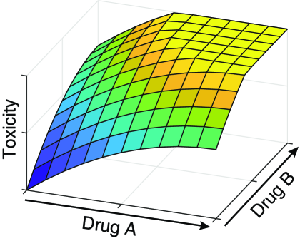
(a) Synergistic.

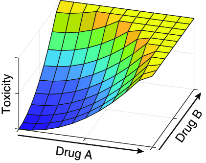
(b) Antagonistic.

Figure 1: Examples of drug-drug interactions.

In joint dose-toxicity models, the drug-drug interaction such as synergy and antagonism shown in Fig. 1 should be captured. To this end, various joint dose-toxicity models have been proposed in the literature as in Table 7. In some models, the joint dose-toxicity model is defined by using the marginal model (i.e., $\pi_{1}(j,{\boldsymbol{\alpha}})$ and $\pi_{2}(k,{\boldsymbol{\beta}})$). In this case, any dose-toxicity model for a single drug such as two-parameter logistic model can be used. In the logistic model, the standardized dosage levels are used (i.e., $d_{j}$ and $u_{k}$ do not indicate actual dosage levels). Thus, there is a parameter $\zeta$ that is not related to any drugs to ensure the appropriate toxicity modeling (Riviere et al.,, 2014). All the models except for the no interaction model can capture the drug-drug interaction and the parameter ${\boldsymbol{\gamma}}$ implies the characteristics of the interaction. For the detailed description and discussion on drug-drug interactions, we refer the readers to (Gasparini,, 2013).

Table 7: Summary of joint dose-toxicity models

Model	$\pi(j,k,{\boldsymbol{\theta}})$
No interaction	$1-\{1-\pi_{1}(j,{\boldsymbol{\alpha}})\}\{1-\pi_{2}(k,{\boldsymbol{\beta}})\}$
Constant log-odds difference	$\frac{1}{1+\gamma^{-1}[\{\pi_{1}(j,{\boldsymbol{\alpha}})+\pi_{2}(k,{\boldsymbol{\beta}})-\pi_{1}(j,{\boldsymbol{\alpha}})\pi_{2}(k,{\boldsymbol{\beta}})\}^{-1}-1]}$
Copula-based (Yin and Yuan, 2009a, )	$1-C\{1-\pi_{1}(j,{\boldsymbol{\alpha}}),1-\pi_{2}(k,{\boldsymbol{\beta}}),\gamma\}$
Thall (Thall et al.,, 2003)	$\frac{\alpha_{1}d_{j}^{\alpha_{2}}+\beta_{1}u_{k}^{\beta_{2}}+\gamma\alpha_{1}d_{j}^{\alpha_{2}}\beta_{1}u_{k}^{\beta_{2}}}{1+\alpha_{1}d_{j}^{\alpha_{2}}+\beta_{1}u_{k}^{\beta_{2}}+\gamma\alpha_{1}d_{j}^{\alpha_{2}}\beta_{1}u_{k}^{\beta_{2}}}$
Exponential	$1-\exp\{-(\alpha d_{j}+\beta u_{k}+\alpha\beta\gamma d_{j}u_{k})\}$
Logistic (Riviere et al.,, 2014)	$\frac{1}{1-\exp(-\zeta-\alpha d_{j}-\beta u_{k}-\gamma d_{j}u_{k})}$

B Proof of Proposition 1

From the definition of $F_{a}^{\mathcal{O}}(v)$, in round $t$, we have

$$\mathbb{P}\left[\left.p_{a}({\boldsymbol{\theta}})\leq F_{a}^{\mathcal{O}(t)}(v)\right|\mathcal{O}(t)\right]=v.$$

Note that the event $\bigcap_{\tau=1}^{t}\left\{\left.p_{a(\tau)}({\boldsymbol{\theta}})\leq F_{a(\tau)}({\boldsymbol{\theta}})^{\mathcal{O}(t)}(v)\right|\mathcal{O}(t)\right\}$ is a subset of the event $\left\{\left.\sum_{\tau=1}^{t}p_{a(\tau)}({\boldsymbol{\theta}})\leq\sum_{\tau=1}^{t}F_{a}^{\mathcal{O}(t)}(v)\right|\mathcal{O}(t)\right\}$ clearly. Then, with $v=(1-\delta)^{1/t}$, we have

$$\mathbb{P}\left[\left.\sum_{\tau=1}^{t}p_{a(\tau)}({\boldsymbol{\theta}})\leq\sum_{\tau=1}^{t}F_{a(\tau)}^{\mathcal{O}(t)}(v)\right|\mathcal{O}(t)\right]\geq\prod_{\tau=1}^{t}\mathbb{P}\left[\left.p_{a(\tau)}({\boldsymbol{\theta}})\leq F_{a(\tau)}^{\mathcal{O}(t)}(v)\right|\mathcal{O}(t)\right]=v^{t}=1-\delta.$$

From the proposition, the residual is non-negative, which implies that $(\xi+\epsilon_{s})t\geq\sum_{\tau=1}^{t}F_{a}^{\mathcal{O}(t)}(v)$. We then have

$$\mathbb{P}\left[\left.\sum_{\tau=1}^{t}p_{a(\tau)}({\boldsymbol{\theta}})\leq(\xi+\epsilon_{s})t\right|\mathcal{O}(t)\right]\geq\mathbb{P}\left[\left.\sum_{\tau=1}^{t}p_{a(\tau)}({\boldsymbol{\theta}})\leq\sum_{\tau=1}^{t}F_{a(\tau)}^{\mathcal{O}(t)}(v)\right|\mathcal{O}(t)\right]\geq 1-\delta.$$

C StructMAB: Safe DC-Finding Bandits Based on Dose-Toxicity Structure

C.1 DC-Finding Bandits Based on Structured Bandits

In our manuscript, we propose a DC-finding algorithm which allows the agent to effectively find the best recommendation for the MTD. To this end, our algorithm exploits a dose-toxicity structure for the drugs from the joint dose-toxicity model. Moreover, it is able to exploit arbitrary joint dose-toxicity models to ensure its practical use. Since the conventional MAB-based dose-finding clinical trial algorithm in Aziz et al., (2019) does not consider the dose-toxicity structure for drug combinations, we develop an advanced MAB-based algorithm by using structured bandits (Gupta et al.,, 2019).

We first define a confidence set for the parameters as

$$\hat{\Theta}(t)\coloneqq\left\{{\boldsymbol{\theta}}:\forall a\in\mathcal{C},~{}|\bar{p}_{a}(t)-p_{a}({\boldsymbol{\theta}})|<\sqrt{\frac{\alpha\log t}{2n_{a}(t)}}\right\},$$ (6)

where $\bar{p}_{a}(t)$ is the empirical toxicity of DC $a$ in round $t$ and $n_{a}(t)$ is the number of observed samples for DC $a$ until round $t$. Since there is no assumption on the parameters ${\boldsymbol{\theta}}$, this confidence set can be obtained for arbitrary joint dose-toxicity models. Then, by using the confidence set, we define a set of candidate MTDs as

$$\mathcal{A}(t)\coloneqq\left\{a\in\mathcal{C}:\mathop{\rm argmin}_{a^{\prime}\in\mathcal{C}}|p_{a^{\prime}}({\boldsymbol{\theta}})-\xi|\textrm{ for some }{\boldsymbol{\theta}}\in\hat{\Theta}(t)\right\}.$$ (7)

For the candidate MTDs, we choose the DC by using Thompson sampling. To this end, we assume that the expected toxicity of the DCs, $p_{a}$’s, are random variables. The posterior probability of the expected toxicity of DC $a$ in round $t$ is updated as $\textrm{Beta}(s_{a}(t)+1,n_{a}(t)-s_{a}(t)+1)$. Then, Thompson sampling is conducted on the set of candidate MTDs as

$$\tilde{p}_{a}(t)\sim\textrm{Beta}(s_{a}(t)+1,n_{a}(t)-s_{a}(t)+1),~{}\forall a\in\mathcal{A}(t).$$ (8)

Based on the samples, the DC whose the sample is closest to the threshold is chosen as

$$a(t)=\mathop{\rm argmin}_{a\in\mathcal{A}(t)}|\tilde{p}_{a}(t)-\xi|.$$ (9)

At the end of the algorithm, the agent chooses the dose whose empirical toxicity is closest to $\xi$ as the MTD

$$\hat{a}^{*}(T)=\mathop{\rm argmin}_{a\in\mathcal{C}}|\bar{p}_{a}(T)-\xi|$$ (10)

or pick $\hat{a}^{*}$ uniformly at random among the allocated doses.

C.2 Safe DC-Finding Bandits

In clinical trials, it is important to avoid testing the unsafe DCs due to the ethical issues. This can be achieved by considering the safety constraint in (1). Here, we propose a safe DC-finding approach that satisfies the safety constraint as in the cautiousness of SDF-Bayes.

For the safe DC-finding approach, we first define a set of conservative DCs as

$$\mathcal{A}_{c}(t)\coloneqq\left\{a\in\mathcal{C}:\max_{{\boldsymbol{\theta}}\in\hat{\Theta}(t)}p_{a}({\boldsymbol{\theta}})\leq\xi\right\}.$$ (11)

The DCs in the set of conservative DCs are safe (i.e., toxicity probability does not exceed the MTD threshold) with a high probability. Thus, by choosing the DCs in the set only, we can avoid the trials with unsafe doses with a high probability. However, this is too conservative and we cannot expect a good MTD recommendation.

To resolve this issue, we consider a residual for the safety constraint in each round. The residual for the safety constraint in round $t$ is defined as

$$r(t)=(\xi+\epsilon_{s})t-\sum_{\tau=1}^{t-1}\max_{{\boldsymbol{\theta}}\in\hat{\Theta}(t)}p_{a(\tau)}({\boldsymbol{\theta}}).$$

Note that the confidence set for the parameters in round $t$, $\hat{\Theta}(t)$, is used for the calculation of the sum of the expected toxicities until round $t$. By using the residual, we can infer whether the safety constraint will be violated or not based on the current confidence set for the parameters. If we still have the non-negative residual with the chosen DC in (9) (i.e., $r(t)-\max_{{\boldsymbol{\theta}}\in\hat{\Theta}(t)}p_{a(t)}({\boldsymbol{\theta}})\geq 0$), then we can expect the safety constraint not to be violated with the chosen DC. Thus, in that case, the safe DC-finding approach accepts the chosen DC, and otherwise, it rejects the chosen DC and chooses the DC in the conservative set $\mathcal{A}_{c}(t)$ instead to ensure the positive residual. We summarize the safe DC-finding algorithm (StructMAB) in Algorithm 2.

Algorithm 2 StructMAB

1:while $t\leq T$ do

2:     Obtain a confidence set $\hat{\Theta}(t)$ as in (6)

3:     Obtain a set of candidate MTDs $\mathcal{A}(t)$ as in (7)

4:     Sample the expected toxicities for all candidate MTDs as in (8)

5:     $\bar{a}\leftarrow\mathop{\rm argmin}_{a\in\mathcal{A}(t)}|\tilde{p}_{a}(t)-\xi|$

6:     if $r(t)-\max_{{\boldsymbol{\theta}}\in\hat{\Theta}(t)}p_{\bar{a}}\geq 0$ then

7:         $a(t)\leftarrow\bar{a}$

8:     else

9:         Obtain a set of conservative DCs $\mathcal{A}_{c}(t)$ as in (11)

10:         Sample the expected toxicities for all conservative DCs

11:         $a(t)\leftarrow\mathop{\rm argmin}_{a\in\mathcal{A}_{c}(t)}|\tilde{p}_{a}(t)-\xi|$

12:     end if

13:     Observe the DLT $Y_{t}$

14:     Update $m_{a(t)}(t+1)$ and $n_{a(t)}(t+1)$

15:     $t\leftarrow t+1$

16:end while

C.3 Sampling-Based Implementation of StructMAB

To use StructMAB in practice, we need to identify the confidence set $\hat{\Theta}$ and the set of candidate MTDs $\mathcal{A}$ based on the confidence set, which requires a high computational complexity in general. Besides, we need different identification methods for different joint dose-toxicity model used in the algorithm. Thus, to resolve these issues, we propose a simple sampling method for StructMAB that can efficiently approximate the confidence set and set of candidate MTDs regardless of which joint dose-toxicity model is used.

Here, we sample ${\boldsymbol{\theta}}$ from the posterior distribution of ${\boldsymbol{\theta}}$, $f({\boldsymbol{\theta}}|\mathcal{O})$, by using Gibbs sampling which is one of most representative Bayesian sampling algorithms for multidimensional sampling as in SDF-Bayes. The posterior distribution of ${\boldsymbol{\theta}}$ can be found in Section 3.1. of our manuscript. Details of the Gibbs sampling procedure can be found in the following section. We denote the number of samples from the posterior distribution $p({\boldsymbol{\theta}}|\mathcal{O}(t))$ by $L$ and the samples by $\tilde{\Theta}(t)=\{{\boldsymbol{\theta}}^{(l)}\}_{l\in[L]}$. Then, from the samples, we can define an approximated confidence set for the parameters as

$$\hat{\Theta}^{\prime}(t)\coloneqq\left\{{\boldsymbol{\theta}}^{(l)}\in\tilde{\Theta}(t):\forall a\in\mathcal{C},~{}|\bar{p}_{a}(t)-p_{a}({\boldsymbol{\theta}}^{(l)})|<\sqrt{\frac{\alpha\log t}{2n_{a}(t)}}\right\}$$

and an approximated set of candidate MTDs as

$$\mathcal{A}^{\prime}(t)\coloneqq\left\{a\in\mathcal{C}:\mathop{\rm argmin}_{a^{\prime}\in\mathcal{C}}|p_{a^{\prime}}({\boldsymbol{\theta}}^{(l)})-\xi|\textrm{ for some }{\boldsymbol{\theta}}^{(l)}\in\hat{\Theta}^{\prime}(t)\right\}.$$ (12)

Similarly, we can define an approximated conservative DCs as

$$\mathcal{A}_{c}^{\prime}(t)\coloneqq\left\{a\in\mathcal{C}:p_{a^{\prime}}({\boldsymbol{\theta}}^{(l)})\leq\xi,~{}\forall{\boldsymbol{\theta}}^{(l)}\in\hat{\Theta}^{\prime}(t)\right\}.$$

We can use these approximated sets for StructMAB. Note that these approximations converges to the true sets as the number of samples goes to infinity. Moreover, for the residual, we use $\max_{{\boldsymbol{\theta}}^{(l)}\in\tilde{\Theta}(t)}p_{a(t)}({\boldsymbol{\theta}}^{(l)})$.

D Description of Sampling Procedure

We describe the sampling procedure used in SDF-Bayes.

• Gibbs sampling: Gibbs sampling is one of the most representative Markov chain Monte Carlo (MCMC) sampling methods to generate a sequence of samples for multiple variables from a multivariate joint probability distribution. In SDF-Bayes, it is used to generate a sequence of samples of the parameter vector ${\boldsymbol{\theta}}=\{\theta_{0},\theta_{1},...,\theta_{D_{\boldsymbol{\theta}}-1}\}$ from $f({\boldsymbol{\theta}}|\mathcal{O})$, where $D_{{\boldsymbol{\theta}}}$ is the dimension of the parameter vector. Note that the dimension of the parameter vector depends on which joint toxicity model is used for SDF-Bayes. In Gibbs sampling, we start from an arbitrary initial sample ${\boldsymbol{\theta}}$ in the distribution. We then samples each component of the parameter vector in turn based on each of the full conditional distribution with updated parameter samples. In Gibbs sampling, we discard $L_{b}$ samples at the beginning which is so-called burn-in period, and then, retain the following $L$ samples. We formally summarize Gibbs sampling as following Algorithm 3.

  Algorithm 3 Gibbs sampling

  1:Initialize ${\boldsymbol{\theta}}^{(0)}$

  2:for $l=1$ to $L_{b}+L$ do

  3:     for $d=0$ to $D_{{\boldsymbol{\theta}}}-1$ do

  4:         Sample $\theta_{d}^{(l)}$ from its full conditional distribution $f\left(\theta_{d}\left|\theta_{0}^{(l)},...,\theta_{d-1}^{(l)},\theta_{d+1}^{(l-1)},...,\theta_{D_{{\boldsymbol{\theta}}}-1}^{(l-1)},\mathcal{O}\right.\right)$

  5:     end for

  6:end for

• Adaptive rejection metropolis sampling: Gibbs sampling relies on the complete full conditional distributions of all components. However, in general, we cannot access to closed forms of such distributions. Thus, in SDF-Bayes, we use adaptive rejection metropolis sampling (ARMS) within Gibbs sampling (Gilks et al.,, 1995). ARMS is a MCMC sampling method as well, and it used to sample from a univariate target distribution specified by (unnormalized) log density.

  Thus, we utilize ARMS to sample each component of the parameter vector from its univariate full conditional distribution (i.e., for line 4 of Algorithm 3). We assume that the prior distributions of the parameters are independent. We denote the parameter vector except for $d$-th component by ${\boldsymbol{\theta}}_{-d}$. Then, we can obtain the unnormalized density of the full conditional distribution of $d$-th parameter, $f(\theta_{d}|{\boldsymbol{\theta}}_{-d}^{\prime},\mathcal{O})$, from the likelihood of ${\boldsymbol{\theta}}$ and the prior distribution as

  $$f(\theta_{d}|{\boldsymbol{\theta}}_{-d}^{\prime},\mathcal{O})\propto L(\theta_{d},{\boldsymbol{\theta}}_{-d}^{\prime}|\mathcal{O})f(\theta_{d})\prod_{d^{\prime}\in\{1,...,d-1,d+1,...D_{{\boldsymbol{\theta}}}\}}f(\theta_{d^{\prime}}^{\prime}).$$

  By using this density, we can sample each component of the parameters within Gibbs sampling. For the detail procedure of ARMS, we refer to (Gilks et al.,, 1995).

E Description of SDF-Bayes-AR

Algorithm 4 SDF-Bayes-AR

1:while $t\leq T$ do

2:     Obtain $a_{m}(t)$’s by SDF-Bayes (lines 2–13)

3:     $g(t)\leftarrow\mathop{\rm argmax}_{m\in\mathcal{M}}\tilde{H}^{\mathcal{O}(t)}_{m,a_{m}(t)}(u)$

4:     $a(t)\leftarrow a_{g(t)}(t)$

5:     Observe DLT $Y_{t}$

6:     Update $s^{g(t)}_{a(t)}(t+1)$ and $n^{g(t)}_{a(t)}(t+1)$

7:     $t\leftarrow t+1$

8:end while

9:Output: $\hat{a}^{*}_{m}\!=\!\mathop{\rm argmax}_{a\in\mathcal{A}}\tilde{G}_{m,a}^{\mathcal{O}(T)}(u),~{}\forall m\!\in\!\mathcal{M}$

F Description of Detailed Experiment Settings

F.1 Real-World Dataset

We describe the real-world dataset used in the experiments. We consider a Phase I drug combination clinical trial dataset and its corresponding dose-toxicity model provided in Bailey et al., (2009). In the dataset, the drug combination of nilotinib and imatinib is considered and the DLT observations from 50 patients are provided to assess the toxicity of different dose combinations. Furthermore, in Bailey et al., (2009), the dose-toxicity model of the combination is constructed in a Bayesian way based on a logistic regression model by using the DLT observations and the prior information about the drugs. In specific, the model is given by

$$\textrm{logit}(d,X_{1},X_{2},X_{3})=\log(\alpha)+\beta\log(d/d^{*})+\xi_{1}X_{1}+\xi_{2}X_{2}+\xi_{3}X_{3},$$

where $\alpha$, $\beta$, $\xi_{n}$’s are dose-toxicity model parameters, $d$ represents the doses of nilotinib and $d^{*}$ is the reference dose of nilotinib (400mg) for scaling. Also, $(X_{1},X_{2},X_{3})$ represents the dose of imatinib by taking the form $(0,0,0)$, $(1,0,0)$, $(1,1,0)$, and $(1,1,1)$ for imatinib doses 0, 400, 600, and 800mg, respectively. The prior distributions of the parameters are tuned by using the historical data such as previous clinical data of each drug without combinations. We rounded up the toxicities at the third decimal place. This trial is originally designed to find the DCs whose toxicities belong to the target interval $(0.20,0.35)$. This implies that the potential DCs of the trial are more conservative in terms of safety (toxicity) compared with typical synthetic datasets designed to find the DC whose toxicity is close to the target toxicity 0.3 because it should find the DCs whose toxicities is lower than 0.3 in average.

F.2 Description of Algorithms in Experiments

Here, we describe the algorithms used in the experiments. We set $u=0.1$ for all the Bayesian algorithms.

• SDF-Bayes: We implement SDF-Bayes based on Algorithm 1 in our manuscript. Here, we provide the settings of SDF-Bayes in the experiments. We set $v=0.9$ unless mentioned. For warm-start of SDF-Bayes, the residual at the early stage of trials can be given by $r(t)=\max\left((\xi+\epsilon_{s})t-\sum_{\tau=1}^{t-1}\tilde{F}_{a(\tau)}^{\mathcal{O}(t)}(v),R\right)$, where $R$ is a constant. Typically, $\xi T$ works well for the cases with a single group. For the joint dose-toxicity model, we use the following logistic dose-toxicity model proposed in Riviere et al., (2014):

  $$\texttt{logit}(\pi_{jk})=\theta_{0}+\theta_{1}u_{j}+\theta_{2}v_{k}+\theta_{3}u_{j}v_{k},$$

  where $\theta_{0}$, $\theta_{1}$, $\theta_{2}$, and $\theta_{3}$ are parameters and $u_{j}$ and $v_{k}$ are the standardized dose of drugs. In the literature (Riviere et al.,, 2014), $u_{j}$’s and $v_{k}$’s are defined as $u_{j}=\log\left(\frac{p_{j}}{1-p_{j}}\right)$ and $v_{k}=\log\left(\frac{q_{k}}{1-q_{k}}\right)$, where $p_{j}$ and $q_{k}$ are the prior estimates of the toxicity probabilities of the $j$-th dosage of drug A and $k$-th dosage of drug B. However, such prior information is not always available, and thus, in the algorithm, we simply use $(-2,-1,0)$ for $u_{j}$’s and $(-3,-2,-1,0)$ for $v_{k}$’s assuming without any prior information. In this model, the parameters are defined as $\theta_{1}>0$ and $\theta_{2}>0$ and $-\infty<\theta_{0}<\infty$. In addition, $\theta_{3}$ should satisfy $\theta_{1}+\theta_{3}v_{k}>0$ and $\theta_{2}+\theta_{3}u_{j}$ for all $k\in\mathcal{K}$ and $j\in\mathcal{J}$. This ensures that the increasing toxicity probability with the increasing dose of a single drug. For the prior of the parameters, we use a normal distribution $\mathcal{N}(0,10)$ for $\theta_{0}$ and $\theta_{3}$. This prior is vague with relatively high variance. For $\theta_{1}$ and $\theta_{2}$, we use an exponential distribution $\textrm{Exp}(1)$ since they are positive. These default prior settings are same with used in the literature (Riviere et al.,, 2014) and used for the other algorithms with the joint dose-toxicity model. For dataset RW, we use $v=0.85$ because the potential DCs of the dataset are designed to be more conservative in terms of safety compared with other datasets as described in the previous section.

• SOTA Bayes (Riviere et al.,, 2014): We implement a Bayesian dose-finding algorithm in Riviere et al., (2014). We denote the probability threshold for dose escalation by $c_{e}$ and the probability threshold for dose de-escalation by $c_{d}$. To avoid that the dose is determined to be escalated and de-escalated at the same time, we need to ensure $c_{e}+c_{d}>1$. We use the joint dose-toxicity model with the same setting from SDF-Bayes for fair comparison. The dose-finding algorithm proposed in Riviere et al., (2014) is described in following:

  • Dose escalation: Let the current DC be $(j,k)$. If $\mathbb{P}[p_{jk}<\xi|\mathcal{O}]>c_{e}$, then the current DC is escalated to an adjacent DC among $\{(j+1,k),(j,k+1),(j+1,k-1),(j-1,k+1)\}$ that has a toxicity probability higher than $p_{jk}$ and closest to $\xi$. If the current DC is the highest one, the same DC is allocated. With the samples from the posterior distribution $f({\boldsymbol{\theta}}|\mathcal{O})$, we approximate the condition as $\frac{1}{L}\sum_{l=1}^{L}\mathbb{I}[p_{jk}({\boldsymbol{\theta}}^{(l)})<\xi]>c_{e}$.

  • Dose de-escalation: Let the current DC be $(j,k)$. If $\mathbb{P}[p_{jk}>\xi|\mathcal{O}]>c_{d}$, then the current DC is de-escalated to an adjacent DC among $\{(j-1,k),(j,k-1),(j+1,k-1),(j-1,k+1)\}$ that has a toxicity probability lower than $p_{jk}$ and closest to $\xi$. If the current DC is the lowest one, the same DC is allocated. With the samples from the posterior distribution $f({\boldsymbol{\theta}}|\mathcal{O})$, we approximate the condition as $\frac{1}{L}\sum_{l=1}^{L}\mathbb{I}[p_{jk}({\boldsymbol{\theta}}^{(l)})>\xi]>c_{d}$.

  • Dose retainment: Let the current DC be $(j,k)$. If $\mathbb{P}[p_{jk}<\xi|\mathcal{O}]\leq c_{e}$ and $\mathbb{P}[p_{jk}>\xi|\mathcal{O}]\leq c_{d}$, the current DC is allocated. With the samples from the posterior distribution $f({\boldsymbol{\theta}}|\mathcal{O})$, we approximate the condition as $\frac{1}{L}\sum_{l=1}^{L}\mathbb{I}[p_{jk}({\boldsymbol{\theta}}^{(l)})<\xi]\leq c_{e}$ and $\frac{1}{L}\sum_{l=1}^{L}\mathbb{I}[p_{jk}({\boldsymbol{\theta}}^{(l)})>\xi]\leq c_{d}$.

  At the end of the trial, the DC recommendation is determined as same with SDF-Bayes.

• StructMAB: We implement StructMAB based on Algorithm 2. For the algorithm, we use the same joint dose-toxicity model and settings for the model used in SDF-Bayes. We set the exploration parameter $\alpha$ in the confidence set for the parameters in (6) to be $1$. Moreover, when constructing the set of candidate MTDs in (12), its condition to include a DC into the set of candidate MTDs is too sensitive in practice since a DC will be included into the set even with only one ground sample that asserts that the DC is optimal. Thus, to mitigate such sensitivity of the condition, we add the following condition: from the set, remove the DCs whose number of ground samples is below the 20% percentile of the number of ground samples of each DC. This helps to remove only the outliers from the set of candidate MTDs. For example, when all the DCs in the set have only one ground sample, then the condition does not remove any DC from the set. Similarly, to avoid StructMAB being too conservative, we use the 80% percentile of the toxicity of the allocated DC among the samples when calculating the residual for the safety constraint.

• IndepTS (Aziz et al.,, 2019): We extend an independent Thompson sampling algorithm in Aziz et al., (2019) for drug combinations. To this end, we simply expand an arm space of IndepTS into two dimensional space for drug combinations. In IndepTS, Thompson sampling is used to estimate the toxicity of DC $a$ as follows:

  $$\tilde{p}_{a}(t)\sim\textrm{Beta}(\alpha_{a}(t),\beta_{a}(t)),$$

  where $\alpha_{a}(t)=s_{a}(t)+1$ and $\beta_{a}(t)=n_{a}(t)-s_{a}(t)+1$. In each round $t$, the expected toxicities of all DCs are sampled based on the above equation. Then, the DC $a(t)$ that has the maximum toxicity sample $\tilde{p}_{a}(t)$ is chosen (i.e., $a(t)=\mathop{\rm argmin}_{a\in\mathcal{C}}|\tilde{p}_{a}(t)-\xi|$). At the end of the trial, it recommends a DC as: $\hat{a}^{*}(T)=\mathop{\rm argmin}_{a\in\mathcal{C}}|\hat{p}_{s,k}(T)-\xi|$. Note that the implicit safety consideration in IndepTS is not exploited in IndepTS-DC since it is for a single drug.

   

• SDF-Bayes-AR: We implement SDF-Bayes-AR based on Algorithm 4 in this supplementary material. In a practical implementation of SDF-Bayes-AR, we adopt uniform patient recruitment in an early phase of clinical trial with the rounds $t\leq T/4$. This enables a warm-start of adaptive patient recruitment and avoids biased recruitment. In addition, we adopt an early stopping strategy to adaptive patient recruitment that has been widely considered in clinical literatures (Riviere et al.,, 2014). If the posterior probability of the most likely DC to be the MTD for group $m$ exceeds a threshold (i.e., $\max_{a\in\mathcal{C}}\tilde{G}_{m,a}^{\mathcal{O}(t)}(u)>p_{es}$, where $p_{e}s$ is the threshold), then SDF-Bayes-AR stops recruiting the patients from group $m$. This prevents unnecessary patient recruitment for the groups whose MTD is confidently discovered.

• SOTA Bayes-AR: We implement SOTA Bayes-AR by adopting our proposed adaptive patient recruitment (AR) to SOTA Bayes. For this, we can simply change line 2 in Algorithm 4 as “Obtain $a_{m}(t)$’s by SOTA Bayes”.

F.3 Experiments with Heterogeneous Groups

Table 8: True toxicity of EP

	Synthetic EP
	1	2	3	4
3	0.12	0.21	0.30	0.40
2	0.075	0.125	0.215	0.30
1	0.035	0.09	0.125	0.205

In the experiments with heterogeneous groups, we apply the Bayesian algorithms to the entire population by treating it as a single group called EP. The toxicity probabilities for EP are the averages of the toxicity probabilities for group A and B, which are provided in Table 8. In the results, the safety violations of each group and the entire trial are considered. For each simulated trial, the safety violation of each group occurs if $S_{m}(T)>\xi+\epsilon$ as described in Section 4.1. On the other hand, the safety violation of the entire trial occurs if $\frac{1}{T}\sum_{t=1}^{T}Y_{t}>\xi+\epsilon$. For prior information, we run a simulated trial for group B with $T_{p}$ patients using SDF-Bayes. Then, we use the observations from the simulated trial as the prior information.

G More Experiment Results with Homogeneous Group

G.1 DLT Observation Rates with Datasets and Distribution of DLT Observation Rates

Table 9: DLT observation rates with datasets A,B,C,D,RW.

	Synthetic A	Synthetic B	Synthetic C	Synthetic D	Real-World
SDF-Bayes	0.296$\pm$.001	0.245$\pm$.001	0.286$\pm$.001	0.305$\pm$.001	0.274$\pm$.001
DF-Bayes	0.342$\pm$.002	0.260$\pm$.001	0.343$\pm$.001	0.351$\pm$.001	0.303$\pm$.001
SOTA Bayes	0.268$\pm$.001	0.204$\pm$.001	0.268$\pm$.001	0.275$\pm$.001	0.238$\pm$.001
StructMAB	0.282$\pm$.001	0.184$\pm$.001	0.279$\pm$.001	0.301$\pm$.001	0.238$\pm$.001
IndepTS	0.239$\pm$.001	0.118$\pm$.001	0.233$\pm$.001	0.278$\pm$.001	0.176$\pm$.001

From Table 9, SDF-Bayes satisfies the safety constraint but it does not achieve the lowest DLT observation rate because it is more often testing DC’s that are believed close to being unsafe; this allows it to more effectively find the true MTD. This exploration-toxicity trade-off can be seen even more clearly by looking at the distribution of DLT observation rates in the following.

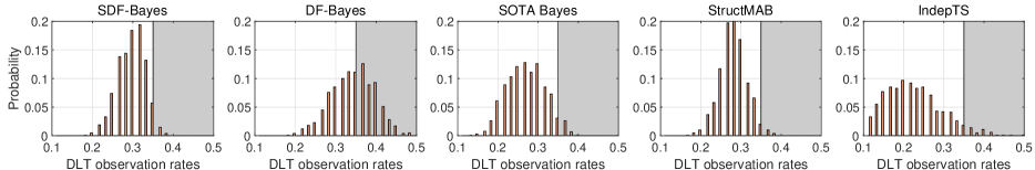
Figure 2: The distribution of DLT observation rates. The region shaded in gray is the region of the DLT observation rates that violate the safety constraint.

In Fig. 2, we provide the histogram of the DLT observation rates of the trials with synthetic dataset A. From the figure, we can see that the DLT observation rates with SDF-Bayes are distributed close to the safety threshold, but only a few trials violate the safety constraint. This clearly shows that SDF-Bayes effectively balances the trade-off between the exploration of the toxicities of the DCs and the DLT observation as intended in its cautious optimism. On the other hand, DF-Bayes frequently violates the safety constraint. This shows the effectiveness of the risk management by the cautiousness in SDF-Bayes. The safety constraint is rarely violated with SOTA Bayes as much as SDF-Bayes. However, their DLT observation rates do not concentrate as in SDF-Bayes since its dose escalation does not have a capability to balance the trade-off explicitly. StructMAB has the similar distribution of DLT observation rates with SDF-Bayes, since the cautiousness principle of SDF-Bayes is adopted in StructMAB. The DLT observation rates of IndepTS are distributed over a low rate region since it fails to estimate the toxicities of DCs.

G.2 DC Allocation Ratios

Figure 3: Heatmaps for DC allocation ratios of Bayesian algorithms. The regions with blue, green, and black borders are underdosing, target-dose, and overdosing regions, respectively.

Fig. 3 shows heatmaps for the DC allocation ratios of the Bayesian algorithms. We can see that the optimism of DF-Bayes results in allocating the most DCs to the target-dose and overdosing. SOTA Bayes concentrates DCs near the MTD $(3,2)$ because of the way it escalates doses. On the other hand, SDF-Bayes allocates DCs in a less concentrated fashion because it tempers its optimism with caution. The result is that SDF-Bayes obtains more information than the other algorithms (and hence makes fewer recommendation errors) while managing risk better.

G.3 Results with More Toxicity Probability Models

Table 10: Synthetic models.

	Synthetic E				Synthetic F				Synthetic G				Synthetic H				Synthetic I
	1	2	3	4	1	2	3	4	1	2	3	4	1	2	3	4	1	2	3	4
3	0.15	0.30	0.45	0.50	0.10	0.15	0.35	0.50	0.17	0.35	0.45	0.50	0.10	0.15	0.25	0.40	0.10	0.25	0.40	0.60
2	0.09	0.12	0.15	0.30	0.07	0.12	0.16	0.35	0.10	0.17	0.35	0.45	0.07	0.12	0.16	0.25	0.07	0.12	0.25	0.40
1	0.05	0.08	0.10	0.13	0.03	0.06	0.08	0.10	0.05	0.10	0.17	0.35	0.03	0.06	0.08	0.10	0.03	0.08	0.18	0.25

Table 11: Safety constraint violation rates and DC recommendation error rates with different datasets.

	Synthetic E		Synthetic F		Synthetic G		Synthetic H		Synthetic I
Algorithms	Safety vio.	Errors	Safety vio.	Errors	Safety vio.	Errors	Safety vio.	Errors	Safety vio.	Errors
SDF-Bayes	0.010$\pm$.002	0.295$\pm$.011	0.006$\pm$.002	0.251$\pm$.010	0.035$\pm$.004	0.285$\pm$.011	0.003$\pm$.001	0.331$\pm$.011	0.033$\pm$.004	0.298$\pm$.011
DF-Bayes	0.239$\pm$.010	0.235$\pm$.010	0.245$\pm$.010	0.195$\pm$.009	0.530$\pm$.012	0.277$\pm$.010	0.112$\pm$.007	0.359$\pm$.011	0.300$\pm$.011	0.392$\pm$.011
SOTA Bayes	0.005$\pm$.002	0.318$\pm$.011	0.005$\pm$.002	0.214$\pm$.010	0.049$\pm$.005	0.283$\pm$.010	0.001$\pm$.001	0.338$\pm$.011	0.014$\pm$.003	0.361$\pm$.011
StructMAB	0.001$\pm$.001	0.592$\pm$.011	0.001$\pm$.001	0.547$\pm$.012	0.033$\pm$.004	0.616$\pm$.011	0.000$\pm$.000	0.490$\pm$.012	0.010$\pm$.002	0.445$\pm$.012
IndepTS	0.000$\pm$.000	0.726$\pm$.010	0.000$\pm$.000	0.697$\pm$.011	0.029$\pm$.004	0.632$\pm$.011	0.000$\pm$.000	0.712$\pm$.011	0.004$\pm$.001	0.582$\pm$.011

Here, we introduce 5 more different synthetic datasets to consider various possible combination toxicities. The toxicity probabilities of each synthetic model are summarized in Table 10 and the MTDs are highlighted in bold. Datasets F and G describe the scenarios in which the MTD’s toxicity probability is higher than the target toxicity ($\xi=0.3$) and datasets H and I describe the scenarios in which the MTD’s toxicity probability is lower than the target toxicity. In Table 11, we provide the performance of the algorithms with the additional synthetic model in Table 10. From the results, we can see that in terms of recommendation error rates, SDF-Bayes outperforms SOTA Bayes in datasets E, H, and I. On the other hand, in datasets F and G, SOTA Bayes achieves lower error rates. This is because SDF-Bayes cautiously chooses the DC to be allocated considering the safety violation; it is hard to follow the optimism principle in those datasets because the MTDs have the higher toxicity than the target toxicity. Hence, SDF-Bayes has an advantage in terms of safety as shown in the results of dataset G; SOTA Bayes is very close to the boundary of a failure to satisfy the safety constraint while SDF-Bayes is not. In the results of MAB-based algorithms (i.e., StructMAB and IndepTS), StructMAB outperforms IndepTS in terms of error rates and achieves similar or lower safety violation rates. However, their error rates are too high compared with those of the other Bayesian algorithms.

G.4 Impact of Budgets

Fig. 4 reports the error rate as a function of the total patient budget. We see that in the practical regime of budgets (less than 100), the error rates of the MAB-based algorithms are significantly higher than the Bayesian algorithms. We note that this is even by using StructMAB, which already exploits the dose-toxicity structure to speed up learning. This clearly shows that the Bayesian designs are more suitable than the MAB-based designs in practice in terms of error rates.

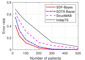
Figure 4: Error rates varying budgets.

Table 12: Performances of SDF-Bayes varying $v$

$v$	Safety vio.	Rec. errors	DLT observ.
0.80	0.135	0.191	0.313
0.85	0.056	0.188	0.313
0.90	0.022	0.203	0.296
0.95	0.005	0.222	0.279

G.5 Impact of Hyperparameter $v$

To show the impact of hyperparameter $v$ on the performance of SDF-Bayes, we provide the performance of SDF-Bayes varying $v$ from 0.80 to 0.95 in Table 12. Note that the hyperparameter $v$ controls how conservative the algorithm is. From the results, we can see that the recommendation error rate increases as $v$ increases. On the other hand, the safety constraint violation rate decreases as $v$ increases. These results clearly show that the hyperparameter $v$ controls the conservativeness of SDF-Bayes well. When $v$ is increasing, SDF-Bayes chooses the DCs more conservatively. Thus, the risk of safety constraint violation decreases. On the other hand, it results in a less exploration. Then, the recommendation error rate increases.

Table 13: Performances of SDF-Bayes varying the prior distribution

Prior	Safety vio.	Rec. errors	DLT observ.
Default	0.023	0.203	0.296
HiVar	0.008	0.212	0.288
NonInfo	0.008	0.208	0.261

G.6 Sensitivity of Prior Distribution

We now provide the performances of SDF-Bayes varying the prior distribution of the parameters of the dose-toxicity model in Table 13. To show the sensitivity of the algorithms, we consider the non-informative prior distribution (NonInfo) (i.e., a uniform distribution) and the distributions with higher variances (HiVar) compared with the prior distributions in our default setting. Specifically, for the non-informative prior, we use a uniform distribution that is truncated according to the domain of each parameter. For the high variance prior, we use a normal distribution $\mathcal{N}(0,50)$ for $\theta_{0}$ and $\theta_{3}$ and use a gamma distribution with mean 1 and variance 10 (i.e., $\Gamma(0.1,0.1)$) for $\theta_{1}$ and $\theta_{2}$.

From the results, we can see that the performance of SDF-Bayes is similar regardless of the prior distribution of the parameters. This implies that SDF-Bayes is robust to the prior distribution since the posterior distribution of the parameters is effectively constructed thanks to the cautious optimism. Beside, it is worth noting that the prior distribution in the default setting is not a precise one as well (Riviere et al.,, 2014). Thus, the case with the non-informative prior distribution is an extreme case in clinical trials for drug combinations since the prior information on the parameters can be usually acquired from historical information, such as laboratory tests and clinical trials for a single drug, and characteristics of dose-combination models. In conclusion, we can use SDF-Bayes in practice even in case with a lack of the prior information of drugs.

Table 14: Performances of SDF-Bayes varying $\psi_{s}$.

$\psi_{s}$	Safety viol. ($\psi_{s}$)	Safety viol. ($\xi+\epsilon_{s}$)	Rec. errors	DLT observ.
0.20	0.048	0.000	0.421	0.169
0.25	0.056	0.000	0.328	0.221
0.30	0.022	0.000	0.257	0.263
0.35	0.019	0.019	0.203	0.297
0.40	0.027	0.193	0.193	0.321

G.7 Impact of Target Safety

In clinical trials, the target toxicity threshold is a standard of safety, and thus, the target safety is usually defined by the target toxicity threshold $\xi$ ($\xi+\epsilon_{s}$ in our manuscript). In SOTA Bayes, dose (de-)escalation is determined based on the target toxicity threshold. Thus, its safety naturally focuses on the target toxicity threshold, and the target safety threshold cannot be arbitrarily determined. On the other hand, SDF-Bayes can consider arbitrary target safety $\psi_{s}$ in its cautious principle by substituting the safety threshold, $\xi+\epsilon_{s}$, in residual $r(t)$ and the set of conservatice DCs $\mathcal{A}_{c}(t)$ in our manuscript, respectively, to any other target safety $\psi_{s}$.

Here, we show the impact of the safety threshold on SDF-Bayes. In Table 14, the recommendation error rates, the safety violation rates with $\psi_{s}$, the safety violation rates with $\xi+\epsilon_{s}$, and the DLT observation rates are provided. From the table, we can see that the safety violation rates with $\psi_{s}$ are similar regardless of the target safety, $\psi_{s}$. This implies that SDF-Bayes effectively manages the risk of safety violation for any given target safety. Consequently, the DLT observation rates increase according to the target safety. This effective risk management in SDF-Bayes makes the target safety $\psi_{s}$ become a safety budget for the exploration of the toxicities of the DCs. Thus, the larger $\psi_{s}$ allows SDF-Bayes to choose the DCs more optimistically during clinical trials. Consequently, in the results, the recommendation error rates decreases as $\psi_{s}$ increases. However, the target safety satisfying $\psi_{s}>\xi+\epsilon_{s}$ is hard to use in practice since the safety violation rate with the standard target safety in clinical trials (i.e., $\xi+\epsilon_{s}$) significantly increases. On the other hand, the target safety satisfying $\psi_{s}<\xi+\epsilon_{s}$ can be used to make trials safer while sacrificing the error rates.

G.8 Runtime and Scalability of SDF-Bayes

We evaluated runtime of SDF-Bayes in our simulations with homogeneous group; on average, it took approximately 2.7 milliseconds to complete a one-round update. (The implementation employed MATLAB with Intel Core i7-8700 3.2GHz CPU but without parallel computing.) By contrast, in a clinical trial, it takes days or weeks (sometimes months) to enroll patients for each round. Besides, actual clinical trials have limited numbers of patients and drug combinations. Even if the trial allowed for a large number of patients, testing hundreds of drug combinations would not be realistic because of safety issues. Hence, the runtime of SDF-Bayes is short enough that it can be used in any realistic trial.

H More Experiment Results with Heterogeneous Groups

H.1 Understanding of Behavior of Bayesian Algorithms Applied to Entire Population

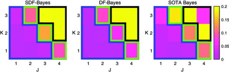
Figure 5: Heatmaps for DC allocation ratios of the patients of group A with the Bayesian algorithms applied to entire population.

Given the toxicities of group EP, the toxicities to group A are under-estimated because the toxicities to group B are very low. As a result, SDF-Bayes and DF-Bayes choose the DCs close to the MTDs of the averaged synthetic model for the entire population (i.e., (2,4) and (3,3) as shown in Table 8). Also, SOTA Bayes escalates dose above the MTDs of group A. These imply that the algorithms applied to group EP frequently select overdosing DCs for the patients of group A; see Fig. 5. Then, as shown in Table 4 in the manuscript, the safety violation rates of group A become excessively high.

H.2 Expected Improvements and Patient Recruitment Ratios

To understand the recruitment behavior of SDF-Bayes-AR, Fig. 6 plots the expected improvement (EI) probability for the most likely DC for each group and the patient recruitment ratio of each group as a function of the amount of prior information ($T_{p}$). The EI for group B decreases as the amount of the prior information increases. (Previous observations render later observations less useful.) SDF-Bayes-UR recruits patients uniformly; SDF-Bayes-AR adaptively recruits patients in order to maximize the EI gain from the next patient.

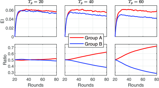
Figure 6: EI of the probability measures and patient recruitments ratio of groups varying the amount of the prior information.

H.3 Results in Section 5.2. with DLT Observation Rates

Here, we provide the DLT observation rates of the results for heterogeneous groups. Tables 15 and 16 provides the DLT observation rates aligned to the results in Tables 3 and 4 in our manuscript, respectively. Table 15 shows that the DLT observation rates of variants of SDF-Bayes are slightly higher than those of SOTA Bayes-UR due to the exploration-toxicity trade-off as in the single group case. (It is shown that they satisfy the safety constraint in Table 3 in our manuscript.) Table 16 shows that SDF-Bayes-AR outperforms SDF-Bayes-UR in terms of total DLT observation rates.

Table 15: DLT observation rates with heterogeneous groups (from Table 3 in the paper).

Algorithms	Total	Group A	Group B
SDF-Bayes-AR	0.263$\pm$.001	0.292$\pm$.001	0.236$\pm$.001
SDF-Bayes-UR	0.263$\pm$.001	0.297$\pm$.001	0.229$\pm$.001
DF-Bayes-UR	0.302$\pm$.001	0.352$\pm$.002	0.252$\pm$.002
SOTA Bayes-UR	0.233$\pm$.001	0.270$\pm$.001	0.196$\pm$.001
SDF-Bayes-EP	0.278$\pm$.001	0.391$\pm$.002	0.166$\pm$.002
DF-Bayes-EP	0.302$\pm$.001	0.427$\pm$.002	0.178$\pm$.002
SOTA Bayes-EP	0.247$\pm$.001	0.352$\pm$.002	0.142$\pm$.001

Table 16: DLT observation rates varying the amount of the prior information (from Table 5 in the paper).

		$T_{p}=20$	$T_{p}=40$	$T_{p}=60$
AR	Group A	0.282$\pm$.001	0.261$\pm$.001	0.250$\pm$.001
	Group B	0.243$\pm$.002	0.259$\pm$.002	0.269$\pm$.003
	Entire	0.262$\pm$.001	0.255$\pm$.001	0.248$\pm$.001
UR	Group A	0.296$\pm$.001	0.296$\pm$.001	0.296$\pm$.001
	Group B	0.238$\pm$.002	0.248$\pm$.002	0.255$\pm$.002
	Entire	0.267$\pm$.001	0.272$\pm$.001	0.275$\pm$.001

References

- Aboutalebi et al., (2019) Aboutalebi, H., Precup, D., and Schuster, T. (2019). Learning modular safe policies in the bandit setting with application to adaptive clinical trials. arXiv preprint arXiv:1903.01026.
- Atan et al., (2019) Atan, O., Zame, W. R., and Schaar, M. (2019). Sequential patient recruitment and allocation for adaptive clinical trials. In Proceedings of the 22nd International Conference on Artificial Intelligence and Statistics (AISTATS).
- Aziz et al., (2019) Aziz, M., Kaufmann, E., and Riviere, M.-K. (2019). On multi-armed bandit designs for dose-finding clinical trials. arXiv preprint arXiv:1903.07082.
- Bagatell et al., (2014) Bagatell, R., Norris, R., Ingle, A. M., Ahern, C., Voss, S., Fox, E., Little, A. R., Weigel, B. J., Adamson, P. C., and Blaney, S. (2014). Phase 1 trial of temsirolimus in combination with irinotecan and temozolomide in children, adolescents and young adults with relapsed or refractory solid tumors: a children’s oncology group study. Pediatric blood & cancer, 61(5):833–839.
- Bailey et al., (2009) Bailey, S., Neuenschwander, B., Laird, G., and Branson, M. (2009). A bayesian case study in oncology phase I combination dose-finding using logistic regression with covariates. Journal of biopharmaceutical statistics, 19(3):469–484.
- Bamias et al., (2011) Bamias, A., Aravantinos, G., Kastriotis, I., Alivizatos, G., Anastasiou, I., Christodoulou, C., Gyftaki, R., Kalofonos, H. P., and Dimopoulos, M. A. (2011). Report of the long-term efficacy of two cycles of adjuvant bleomycin/etoposide/cisplatin in patients with stage I testicular nonseminomatous germ-cell tumors (NSGCT): a risk adapted protocol of the Hellenic Cooperative Oncology Group. Urologic Oncology: Seminars and Original Investigations, 29(2):189–193.
- Berry, (2006) Berry, D. A. (2006). Bayesian clinical trials. Nature reviews Drug discovery, 5(1):27.
- Bubeck and Cesa-Bianchi, (2012) Bubeck, S. and Cesa-Bianchi, N. (2012). Regret analysis of stochastic and nonstochastic multi-armed bandit problems. Foundations and Trends in Machine Learning, 5(1):1–122.
- Calvo et al., (2017) Calvo, E., Soria, J.-C., Ma, W. W., Wang, T., Bahleda, R., Tolcher, A. W., Gernhardt, D., O’Connell, J., Millham, R., Giri, N., et al. (2017). A phase I clinical trial and independent patient-derived xenograft study of combined targeted treatment with dacomitinib and figitumumab in advanced solid tumors. Clinical Cancer Research, 23(5):1177–1185.
- Dasari et al., (2013) Dasari, A., Gore, L., Messersmith, W., Diab, S., Jimeno, A., Weekes, C., Lewis, K., Drabkin, H., Flaig, T., and Camidge, D. (2013). A phase I study of sorafenib and vorinostat in patients with advanced solid tumors with expanded cohorts in renal cell carcinoma and non-small cell lung cancer. Investigational new drugs, 31(1):115–125.
- Flaherty et al., (2012) Flaherty, K. T., Infante, J. R., Daud, A., Gonzalez, R., Kefford, R. F., Sosman, J., Hamid, O., Schuchter, L., Cebon, J., Ibrahim, N., et al. (2012). Combined BRAF and MEK inhibition in melanoma with BRAF V600 mutations. New England Journal of Medicine, 367(18):1694–1703.
- Garivier et al., (2017) Garivier, A., Ménard, P., Rossi, L., and Menard, P. (2017). Thresholding bandit for dose-ranging: The impact of monotonicity. arXiv preprint arXiv:1711.04454.
- Gasparini, (2013) Gasparini, M. (2013). General classes of multiple binary regression models in dose finding problems for combination therapies. Journal of the Royal Statistical Society: Series C (Applied Statistics), 62(1):115–133.
- Gilks et al., (1995) Gilks, W. R., Best, N. G., and Tan, K. (1995). Adaptive rejection metropolis sampling within Gibbs sampling. Journal of the Royal Statistical Society: Series C (Applied Statistics), 44(4):455–472.
- Gupta et al., (2019) Gupta, S., Chaudhari, S., Mukherjee, S., Joshi, G., and Yağan, O. (2019). A unified approach to translate classical bandit algorithms to the structured bandit setting. arXiv preprint arXiv:1810.08164.
- Hamberg et al., (2010) Hamberg, P., Ratain, M. J., Lesaffre, E., and Verweij, J. (2010). Dose-escalation models for combination phase I trials in oncology. European Journal of Cancer, 46(16):2870–2878.
- Hobbs et al., (2011) Hobbs, B. P., Carlin, B. P., Mandrekar, S. J., and Sargent, D. J. (2011). Hierarchical commensurate and power prior models for adaptive incorporation of historical information in clinical trials. Biometrics, 67(3):1047–1056.
- Kelly and Halabi, (2018) Kelly, W. K. and Halabi, S. (2018). Oncology clinical trials: successful design, conduct, and analysis. Springer Publishing Company.
- Kim et al., (2009) Kim, T., Sym, S., Lee, S., Ryu, M., Lee, J., Chang, H., Kim, H., Shin, J., Kang, Y., and Lee, J. (2009). A UGT1A1 genotype-directed phase I study of irinotecan (CPT-11) combined with fixed dose of capecitabine in patients with metastatic colorectal cancer (mCRC). Journal of Clinical Oncology, 27(15_suppl):2554–2554.
- Lee et al., (2020) Lee, H.-S., Shen, C., Jordon, J., and van der Schaar, M. (2020). Contextual constrained learning for dose-finding clinical trials. In Proceedings of the 23rd International Conference on Artificial Intelligence and Statistics (AISTATS).
- Moss et al., (2015) Moss, R. B., Flume, P. A., Elborn, J. S., Cooke, J., Rowe, S. M., McColley, S. A., Rubenstein, R. C., and Higgins, M. (2015). Efficacy and safety of ivacaftor treatment: randomized trial in subjects with cystic fibrosis who have an R117H-CFTR mutation. The Lancet. Respiratory medicine, 3(7):524.
- Ocana et al., (2019) Ocana, A., Gil-Martin, M., Antolín, S., Atienza, M., Montaño, Á., Ribelles, N., Urruticoechea, A., Falcón, A., Pernas, S., Orlando, J., et al. (2019). Efficacy and safety of dasatinib with trastuzumab and paclitaxel in first line HER2-positive metastatic breast cancer: results from the phase II GEICAM/2010-04 study. Breast cancer research and treatment, 174(3):693–701.
- O’Quigley et al., (1990) O’Quigley, J., Pepe, M., and Fisher, L. (1990). Continual reassessment method: a practical design for phase 1 clinical trials in cancer. Biometrics, pages 33–48.
- Paller et al., (2019) Paller, C. J., Huang, E., Luechtefeld, T., Masset, H., Williams, C., Zhao, J., Gravell, A., Tamashiro, T., Reeves, S., Rosner, G., et al. (2019). Factors affecting combination trial success (FACTS): Investigator survey results on early-phase combination trials. Frontiers in Medicine, 6:122.
- Pallmann et al., (2018) Pallmann, P., Bedding, A. W., Choodari-Oskooei, B., Dimairo, M., Flight, L., Hampson, L. V., Holmes, J., Mander, A. P., Sydes, M. R., Villar, S. S., et al. (2018). Adaptive designs in clinical trials: why use them, and how to run and report them. BMC medicine, 16(1):29.
- Park et al., (2018) Park, J. J., Thorlund, K., and Mills, E. J. (2018). Critical concepts in adaptive clinical trials. Clinical epidemiology, 10:343.
- Plummer et al., (2008) Plummer, R., Jones, C., Middleton, M., Wilson, R., Evans, J., Olsen, A., Curtin, N., Boddy, A., McHugh, P., Newell, D., et al. (2008). Phase I study of the poly (ADP-ribose) polymerase inhibitor, AG014699, in combination with temozolomide in patients with advanced solid tumors. Clinical cancer research, 14(23):7917–7923.
- Riviere et al., (2014) Riviere, M.-K., Yuan, Y., Dubois, F., and Zohar, S. (2014). A bayesian dose-finding design for drug combination clinical trials based on the logistic model. Pharmaceutical statistics, 13(4):247–257.
- Shen et al., (2020) Shen, C., Wang, Z., Villar, S., and van der Schaar, M. (2020). Learning for dose allocation in adaptive clinical trials with safety constraints. In Proceedings of International Conference on Machine Learning (ICML).
- Shen et al., (2019) Shen, Y., Liu, T., Chen, J., Li, X., Liu, L., Shen, J., Wang, J., Zhang, R., Sun, M., Wang, Z., et al. (2019). Harnessing artificial intelligence to optimize long-term maintenance dosing for antiretroviral-naive adults with HIV-1 infection. Advanced Therapeutics, page 1900114.
- Sun and Braun, (2015) Sun, Z. and Braun, T. M. (2015). A two-dimensional biased coin design for dual-agent dose-finding trials. Clinical Trials, 12(6):596–607.
- Thall et al., (2003) Thall, P. F., Millikan, R. E., Mueller, P., and Lee, S.-J. (2003). Dose-finding with two agents in phase I oncology trials. Biometrics, 59(3):487–496.