Sample path generation of the stochastic volatility CGMY process and its application to path-dependent option pricing

Abstract

This paper proposes the sample path generation method for the stochastic volatility version of CGMY process. We present the Monte-Carlo method for European and American option pricing with the sample path generation and calibrate model parameters to the American style S&P 100 index options market, using the least square regression method. Moreover, we discuss path-dependent options such as Asian and Barrier options.

1 Introduction

Since Heston (1993) applied the CIR model by Cox et al. (1985) to option pricing, the model has been the standard framework for option pricing because it allows for stochastic volatility and volatility smile effect that observed for the Black Scholes model (Black and Scholes (1973)). However, the Lévy process models with time-varying volatility have been used in option pricing in descrete time model, since empirical studies based on the stochastic volatility model show that the Brownian Motion is often rejected (See Rachev and Mittnik (2000), Kim et al. (2010), Kim et al. (2011)). Carr et al. (2003) defined the class of continuous time stochastic volatility model on Lévy processes (SVLP) using the time changed Lévy process. The SVLP has been successfully applied in European option pricing, but the absence of an efficient sample path generation method makes the SVLP model hard to be applied to path-dependent options such as American, Barrier or Asian option.

This paper proposes the sample path generation method for the stochastic volatility version of CGMY (CGMYSV) process, which is a subclass of the SVLP model. The method is constructed by an approximation of the series representation of CGMY process with the time-varying scale parameter. The series representations for the tempered stable and tempered infinitely divisible processes are discussed in Rosiński (2007) and Bianchi et al. (2010), and it is applied to Monte-Carlo simulation for CGMY market model with a GARCH volatility in Kim et al. (2010). Yet, the CGMYSV model is a continuous-time model different from the GARCH model with CGMY innovations. We develop an algorithm of the CGMYSV sample path generation, and it will be applied Monte-Carlo simulation (MCS). The algorithm will be used to price European and American option and to calibrate risk-neutral parameters to the S&P 500 index option (European style) and S&P 100 option (American style) data. We will use the least square regression method by Longstaff and Schwartz (2001) for American option pricing with MCS. We verify that the new sample path generation method performs well in American option pricing by that empirical study. We also apply the algorithm to Asian and Barrier option pricing with MCS.

The remainder of this paper is organized as follows. The CIR process and the CGMY process with the series representation are presented in Section 2. The sample path generation method based on the series representation is constructed in Section 3. In Section 4, we perform the CGMYSV model calibration for S&P 500 index option and S&P 100 index option. Also, the Asian and Barrier option prices are discussed. Finally, Section 6 concludes.

2 Preliminary

In this section, we briefly discuss CIR model and CGMY process.

2.1 CIR model

The CIR model is given by

$$dv_{t}=\kappa(\eta-v_{t})dt+\zeta\sqrt{v_{t}}dW_{t}\text{ and }v_{0}>0,$$ (1)

for $\kappa,\eta,\zeta>0$ and Brownian motion $\{W_{t}\}_{t\geq 0}$. Let $\mathcal{F}^{v}_{t}$ be a smallest $\sigma$-algebra generated by process $\{v_{s}\}_{0\leq s\leq t}$ then $v_{t+{\varDelta t}}|_{\mathcal{F}^{v}_{t}}\stackrel{{\scriptstyle\mathrm{d}}}{{=}}\xi/(2c)$ where $c=\frac{2\kappa}{(1-e^{-\kappa{\varDelta t}})\zeta^{2}}$ and the random variable $\xi$ is non-central $\chi^{2}$-distributed with degrees of freedom $4\kappa\eta/\zeta^{2}$ and noncentrality parameter $2cv_{t}e^{-\kappa{\varDelta t}}$.

Let ${\mathcal{V}}_{t}=\int_{0}^{t}v_{s}ds$ then the joint distribution of $\left(v_{t},,{\mathcal{V}}_{t}\right)$ is characterized by the characteristic function $\Phi_{t}(a,b,x)=E\left[\exp(a{\mathcal{V}}_{t}+ibv_{t})|v_{0}=x\right]$ given as following (Proposition 6.2.5 in Lamberton and Lapeyre (1996))

$$\Phi_{t}(a,b,x)=A(t,a,b)\exp\left(B(t,a,b)x\right)$$ (2)

with

$$A(t,a,b) =\frac{\exp\left(\frac{\kappa^{2}\eta t}{\zeta^{2}}\right)}{\left(\cosh\left(\frac{\gamma t}{2}\right)+\frac{\kappa-ib\zeta^{2}}{\gamma}\sinh\left(\frac{\gamma t}{2}\right)\right)^{2\kappa\eta/\zeta^{2}}}$$

$$B(t,a,b) =\frac{ib\left(\gamma\cosh\left(\frac{\gamma t}{2}\right)-\kappa\sinh\left(\frac{\gamma t}{2}\right)\right)+2ia\sinh\left(\frac{\gamma t}{2}\right)}{\gamma\cosh\left(\frac{\gamma t}{2}\right)+\left(\kappa-ib\zeta^{2}\right)\sinh\left(\frac{\gamma t}{2}\right)}$$

$$\gamma =\sqrt{\kappa^{2}-2\zeta^{2}ia}.$$

2.2 CGMY Process

For $\alpha\in(0,2)$, $C,\lambda_{+},\lambda_{-}>0$, and $\mu\in\mathbb{R}$, an infinitely divisible random variable $X$ with characteristic function (Ch.F)

$$\phi_{\textup{CGMY}}(u;\alpha,C,\lambda_{+},\lambda_{-},\mu)=\phi_{X}(u)=E[e^{iuX}]$$

$$=\exp\left((\mu-C\Gamma(1-\alpha)(\lambda_{+}^{\alpha-1}-\lambda_{-}^{\alpha-1}))iu-C\Gamma(-\alpha)\left((\lambda_{+}-iu)^{\alpha}-\lambda_{+}^{\alpha}+(\lambda_{-}+iu)^{\alpha}-\lambda_{-}^{\alpha}\right)\right)$$

is referred to as the CGMY distributed random variable with parameters $(\alpha$, $C$, $\lambda_{+}$, $\lambda_{-}$, $\mu)$. In this case, we denote $X\sim\textup{CGMY}(\alpha$, $C$, $\lambda_{+}$, $\lambda_{-}$, $\mu)$.

Let $C=(\Gamma(2-\alpha)(\lambda_{+}^{\alpha-2}+\lambda_{-}^{\alpha-2}))^{-1}$ and $\mu=0$. Then a CGMY random variable $Z\sim\textup{CGMY}(\alpha$, $C$, $\lambda_{+}$, $\lambda_{-}$, $\mu)$ has zero mean ($E[Z]=0$) and unit variance ($\textrm{var}(Z)=1$). In this case, we say that $Z$ is standard CGMY distributed and denote $Z\sim\textup{stdCGMY}(\alpha$, $\lambda_{+}$, $\lambda_{-})$. Moreover, the Ch.F of $Z$ is given by

$$\phi_{\textup{stdCGMY}}(u;\alpha,\lambda_{+},\lambda_{-})=\phi_{Z}(u)=E[e^{iuZ}]$$

$$=\exp\left(\frac{\lambda_{+}^{\alpha-1}-\lambda_{-}^{\alpha-1}}{(\alpha-1)(\lambda_{+}^{\alpha-2}+\lambda_{-}^{\alpha-2})}iu+\frac{(\lambda_{+}-iu)^{\alpha}-\lambda_{+}^{\alpha}+(\lambda_{-}+iu)^{\alpha}-\lambda_{-}^{\alpha}}{\alpha(\alpha-1)(\lambda_{+}^{\alpha-2}+\lambda_{-}^{\alpha-2})}\right).$$ (3)

Since the CGMY distribution is purely non-Gaussian infinitely divisible, it generate a pure jump Lévy process $\{X_{t}\}_{t\geq 0}$ such that $X_{1}$ $\sim$ $\textup{CGMY}(\alpha$, $C$, $\lambda_{+}$, $\lambda_{-}$, $\mu)$. In this case, we say that $(X_{t})_{t\geq 0}$ is CGMY process with parameters $(\alpha$, $C$, $\lambda_{+}$, $\lambda_{-}$, $\mu)$. The characteristic function (Ch.F) of $X_{t}$ is

$$\phi_{X_{t}}(u)=\exp(t\log(\phi_{\textup{CGMY}}(u;\alpha,C,\lambda_{+},\lambda_{-},\mu))).$$

With the same argument, a pure jump Lévyprocess $\{Z_{t}\}_{t\geq 0}$ such that $Z_{1}$ $\sim$ $\textup{stdCGMY}(\alpha$, $\lambda_{+}$, $\lambda_{-})$ is referred to as the standard CGMY process with parameters $(\alpha$, $\lambda_{+}$, $\lambda_{-})$. The CGMY and standard CGMY processes are characterized by their Lévy symbols

$$\psi_{\textup{CGMY}}(u;\alpha,C,\lambda_{+},\lambda_{-},\mu)=\log\phi_{\textup{CGMY}}(u;\alpha,C,\lambda_{+},\lambda_{-},\mu)$$

and

$$\psi_{\textup{stdCGMY}}(u;\alpha,\lambda_{+},\lambda_{-})=\log\phi_{\textup{stdCGMY}}(u;\alpha,\lambda_{+},\lambda_{-}),$$

respectively.

2.3 Series Representation of the CGMY Process

Rosiński (2007) introduced the series representation form for the tempered stable random variable and process, and it can be used for the CGMY sample path generation. Assume that $X\sim\textup{CGMY}(\alpha$, $C$, $\lambda_{+}$, $\lambda_{-}$, $0)$. Let $\{U_{j}\}_{j=1,2,\cdots}$ be an independent and identically distributed (i.i.d.) sequence of uniform random variables on $(0,1)$. Let $\{E_{j}\}_{j=1,2,\cdots}$ be i.i.d. sequences of exponential random variables with parameters 1, and let $\{\Gamma_{j}\}_{j=1,2,\cdots}$ be a Poisson point process with parameter 1. Let $\{V_{j}\}_{j=1,2,\cdots}$ be an i.i.d. sequence of random variables in $\{\lambda_{+},\lambda_{-}\}$ with $P(V_{j}=\lambda_{+})=P(V_{j}=\lambda_{-})=1/2$. Suppose that $\{U_{j}\}_{j=1,2,\cdots}$, $\{V_{j}\}_{j=1,2,\cdots}$, $\{E_{j}\}_{j=1,2,\cdots}$, and $\{\Gamma_{j}\}_{j=1,2,\cdots}$ are independent. Then $X$ represented by the following series form:

$$X=\sum_{j=1}^{\infty}\left[\left(\frac{\alpha\Gamma_{j}}{2C}\right)^{-1/\alpha}\wedge E_{j}U_{j}^{1/\alpha}|V_{j}|^{-1}\right]\frac{V_{j}}{|V_{j}|}+b,$$

where $b=-C\Gamma(1-\alpha)\left(\lambda_{+}^{\alpha-1}-\lambda_{-}^{\alpha-1}\right)$. Let $\{\tau_{j}\}_{j=1,2,\cdots}$ be an i.i.d. sequence of uniform random variables on $(0,T)$ independent of $\{U_{j}\}_{j=1,2,\cdots}$, $\{V_{j}\}_{j=1,2,\cdots}$, $\{E_{j}\}_{j=1,2,\cdots}$, and $\{\Gamma_{j}\}_{j=1,2,\cdots}$. Suppose

$$X_{t}=\sum_{j=1}^{\infty}\left[\left(\frac{\alpha\Gamma_{j}}{2CT}\right)^{-1/\alpha}\wedge E_{j}U_{j}^{1/\alpha}|V_{j}|^{-1}\right]\frac{V_{j}}{|V_{j}|}1_{\tau_{j}\leq t}+tb_{T},~{}~{}~{}t\in[0,T],$$

where $b_{T}=-C\Gamma(1-\alpha)\left(\lambda_{+}^{\alpha-1}-\lambda_{-}^{\alpha-1}\right)$. Then the the process $\{X_{t}\}_{t\in[0,T]}$ is the CGMY process with parameters $(\alpha$, $C$, $\lambda_{+}$, $\lambda_{-}$, $0)$ for the time horizon $T>0$.

3 Stochastic volatility version of the CGMY process

Suppose $\{Z_{t}\}_{t\geq 0}$ is the standard CGMY process with parameters $(\alpha$, $\lambda_{+}$, $\lambda_{-})$ and $\{v_{t}\}$ is the stochastic volatility process given by CIR model in(1). We define a process $\{L_{t}\}_{t\geq 0}$ by

$$L_{t}=Z_{{\mathcal{V}}_{t}}+\rho v_{t}$$ (4)

where ${\mathcal{V}}_{t}=\int_{0}^{t}v_{s}ds$, and $\{Z_{t}\}_{t\geq 0}$ is independent of the process $\{v_{t}\}_{t\geq 0}$. The process $\{L_{t}\}_{t\geq 0}$ is referred to as the stochastic volatility version of the CGMY process or simply CGMYSV process with parameters $(\alpha$, $\lambda_{+}$, $\lambda_{-}$, $\kappa$, $\eta$, $\zeta$, $\rho$, $v_{0})$. By (2), we obtain the characteristic function of $L_{t}$ as

$$\phi_{L_{t}}(u)=\Phi_{t}(-i\psi_{\textup{stdCGMY}}(u;\alpha,\lambda_{+},\lambda_{-}),\rho u,v_{0}),$$ (5)

where $\phi_{\textup{stdCGMY}}(u;\alpha,\lambda_{+},\lambda_{-})$ is the characteristic function of $Z_{1}$ defined in (3).

Result: SVMYSV sample path

Let $T$ be the time horizon ;

Let $M$, $J$, and $N$ be large positive integer ;

$\varDelta t=T/M$, $v_{n,0}=v_{0}$, $c=\frac{2\kappa}{(1-e^{-\kappa{\varDelta t}})\zeta^{2}}$, $C=(\Gamma(2-\alpha)(\lambda_{+}^{\alpha-2}+\lambda_{-}^{\alpha-2}))^{-1}$ ;

$n=1$ ;

while $n\leq N$ do

       $m=1$;

       while $m\leq M$ do

             $\xi=$ non-central $\chi^{2}$-distributed random variable with degrees of freedom $4\kappa\eta/\zeta^{2}$ and noncentrality parameter $2cv_{n,m-1}e^{-\kappa{\varDelta t}}$ ;

             $v_{n,m}=\xi/(2c)$ ;

             $m=m+1$

       end while

      $j=1$, $\Gamma_{0}=0$;

       while $j\leq N$ do

             $U_{j}=$ uniform random numbers on $(0,1)$ ;

             $U^{\prime}_{j}=$ uniform random numbers on $(0,1)$ ;

             $E_{j}=$ exponential random numbers with parameter 1 ;

             $E^{\prime}_{j}=$ exponential random numbers with parameter 1 ;

             $\Gamma_{j}=\Gamma_{j-1}+E_{j}^{\prime}$ ;

             if $U^{\prime}_{j}\leq 0.5$ then

                   $V_{j}=\lambda_{+}$

            else

                   $V_{j}=\lambda_{-}$

             end if

            $\tau_{j}=$ uniform random numbers on $(0,T)$ ;

             $c(\tau_{j})=C\sum_{k=1}^{M}v_{n,k-1}1_{(k-1){\varDelta t}<\tau_{j}\leq k{\varDelta t}}$ ;

             $j=j+1$ ;

            

       end while

      $m=1$, $Y_{n,0}=0$ ;

       while $m\leq M$ do

             $b_{m}=-\frac{v_{n,m-1}\left(\lambda_{+}^{\alpha-1}-\lambda_{-}^{\alpha-1}\right)}{(1-\alpha)(\lambda_{+}^{\alpha-2}+\lambda_{-}^{\alpha-2})}$;

             $Y_{n,m}=Y_{n,m-1}+\sum_{j=1}^{J}\left[\left(\frac{\alpha\Gamma_{j}}{2c(\tau_{j})T}\right)^{-1/\alpha}\wedge E_{j}U_{j}^{1/\alpha}|V_{j}|^{-1}\right]\frac{V_{j}}{|V_{j}|}1_{(m-1){\varDelta t}<\tau_{j}\leq m{\varDelta t}}+b_{m}{\varDelta t}\;$ $L_{n,m}=Y_{n,m}+\rho v_{n,m}$ ;

             $m=m+1$;

            

       end while

      $n=n+1$;

      

end while

Algorithm 1 CGMYSV sample path generation

3.1 Series representation of the CGMYSV Process

Suppose that we have a CIR process $\{v_{t}\}_{t\geq 0}$ with parameters $\kappa,\eta,$ and $\zeta$ as defined in (1), ${\mathcal{V}}_{t}=\int_{0}^{t}v_{s}ds$ for $t>0$, and suppose that $\{\mathcal{F}^{v}_{t}\}_{t\geq 0}$ is natural filtration generated by $\{v_{t}\}_{t\geq 0}$. Let $P=\{0=t_{0}<t_{1}<\cdots<t_{m}<\cdots<M=T\}$ be the partition of time, ${\varDelta t}_{m}=t_{m}-t_{m-1}$ for $m\in\{1,2,\cdots,M\}$, and let $||P||=\max\{{\varDelta t}_{m}\,|\,m=1,2,\cdots,M\}$. Suppose that $\{v_{t_{m}}\}_{t_{m}\in P}$ and $\{L_{t_{m}}\}_{t_{m}\in P}$ are discrete sub-sequences of the CIR process and the CGMYSV process, respectively. Let $\varDelta L_{t_{m}}=L_{t_{m}}-L_{t_{m-1}}$, $\varDelta{\mathcal{V}}_{t_{m}}={\mathcal{V}}_{t_{m}}-{\mathcal{V}}_{t_{m-1}}$, and $\varDelta v_{t_{m}}=v_{t_{m}}-v_{t_{m-1}}$. Then we have

$$\varDelta L_{t_{m}}|_{\mathcal{F}^{v}_{t_{m-1}}}\stackrel{{\scriptstyle\mathrm{d}}}{{=}}(Z_{{\mathcal{V}}_{t_{m}}-{\mathcal{V}}_{t_{m-1}}})|_{\mathcal{F}^{v}_{t_{m-1}}}+\rho(v_{t_{m}}-v_{t_{m-1}})|_{\mathcal{F}^{v}_{t_{m-1}}}=Z_{\varDelta{\mathcal{V}}_{t_{m}}}|_{\mathcal{F}^{v}_{t_{m-1}}}+\rho(\varDelta v_{t_{m}}|_{\mathcal{F}^{v}_{t_{m-1}}}),$$

where

$$Z_{\varDelta{\mathcal{V}}_{t_{m}}}|_{\mathcal{F}^{v}_{t_{m-1}}}\sim\textup{CGMY}\left(\alpha,C(\varDelta{\mathcal{V}}_{t_{m}}|_{\mathcal{F}^{v}_{t_{m-1}}}),\lambda_{+},\lambda_{-},0\right),$$

and $C=\left(\Gamma(2-\alpha)(\lambda_{+}^{\alpha-2}+\lambda_{-}^{\alpha-2})\right)^{-1}$. Since we approximate

$$\varDelta{\mathcal{V}}_{t_{m}}|_{\mathcal{F}^{v}_{t_{m-1}}}=\int_{t_{m-1}}^{t_{m}}v_{t}\,dt\approx v_{t_{m-1}}{\varDelta t}_{m},$$

we have

$$Z_{\varDelta{\mathcal{V}}_{t_{m}}}|_{\mathcal{F}^{v}_{t_{m-1}}}\approx Z_{v_{t_{m-1}}{\varDelta t}_{m}}|_{\mathcal{F}^{v}_{t_{m-1}}}\sim\textup{CGMY}\left(\alpha,Cv_{t_{m-1}}{\varDelta t}_{m},\lambda_{+},\lambda_{-},0\right).$$

Suppose $\{Y_{t_{m}}\}_{t_{m}\in P}$ is a process defined by

$$Y_{t_{m}}=Y_{t_{m-1}}+Z_{v_{t_{m-1}}{\varDelta t}_{m}}|_{\mathcal{F}^{v}_{t_{m-1}}},~{}~{}~{}m=1,2,\cdots,M$$

with $Y_{0}=0$, then $Y_{t_{m}}\approx Z_{{\mathcal{V}}_{t_{m}}}|_{\mathcal{F}^{v}_{t_{m-1}}}$ and $\{Y_{t_{m}}\}_{t_{m}\in P}$ is an approximation of the process $\{Z_{{\mathcal{V}}_{t_{m}}}|_{\mathcal{F}^{v}_{t_{m-1}}}\}_{t_{m}\in P}$.

By the series representation, we have

$$Z_{v_{t_{m-1}}{\varDelta t}_{m}}|_{\mathcal{F}^{v}_{t_{m-1}}}\stackrel{{\scriptstyle\mathrm{d}}}{{=}}\sum_{j=1}^{\infty}\left[\left(\frac{\alpha\Gamma_{j}}{2c_{m}{\varDelta t}_{m}}\right)^{-1/\alpha}\wedge E_{j}U_{j}^{1/\alpha}|V_{j}|^{-1}\right]\frac{V_{j}}{|V_{j}|}+b_{m}{\varDelta t}_{m}$$

where $b_{m}=-c_{m}\Gamma(1-\alpha)\left(\lambda_{+}^{\alpha-1}-\lambda_{-}^{\alpha-1}\right)$, $c_{m}=v_{t_{m-1}}C$, and $\{U_{j}\}_{j=1,2,\cdots}$, $\{V_{j}\}_{j=1,2,\cdots}$, $\{E_{j}\}_{j=1,2,\cdots}$, and $\{\Gamma_{j}\}_{j=1,2,\cdots}$ are given in Section 2.3. The same argument as the relation between series representation of the CGMY process presented in Section 2.3, we can define a series representation of $Y_{t_{m}}$ as follows:

$$Y_{t_{m}}=\sum_{j=1}^{\infty}\left[\left(\frac{\alpha\Gamma_{j}}{2c(\tau_{j})T}\right)^{-1/\alpha}\wedge E_{j}U_{j}^{1/\alpha}|V_{j}|^{-1}\right]\frac{V_{j}}{|V_{j}|}1_{\tau_{j}\leq t_{m}}+\sum_{k=1}^{m}b_{k}{\varDelta t}_{k}$$ (6)

where

$$b_{k}=-\frac{v_{t_{k-1}}\left(\lambda_{+}^{\alpha-1}-\lambda_{-}^{\alpha-1}\right)}{(1-\alpha)(\lambda_{+}^{\alpha-2}+\lambda_{-}^{\alpha-2})},$$

$$c(\tau_{j})=C\sum_{m=1}^{M}v_{t_{m-1}}1_{t_{m-1}<\tau_{j}\leq t_{m}},$$

and $\{\tau_{j}\}_{j=1,2,\cdots}$ is an i.i.d. sequence of uniform random variables on $(0,T)$ independent of $\{U_{j}\}_{j=1,2,\cdots}$, $\{V_{j}\}_{j=1,2,\cdots}$, $\{E_{j}\}_{j=1,2,\cdots}$, and $\{\Gamma_{j}\}_{j=1,2,\cdots}$. Therefore, we have

$$L_{t_{m}}|_{\mathcal{F}^{v}_{t_{m-1}}}=Z_{{\mathcal{V}}_{t_{m}}}|_{\mathcal{F}^{v}_{t_{m-1}}}+\rho v_{t_{m}}|_{\mathcal{F}^{v}_{t_{m-1}}}\approx Y_{t_{m}}+\rho v_{t_{m}}|_{\mathcal{F}^{v}_{t_{m-1}}}.$$ (7)

Combining equations (6) and (7), we can generate sample path of the CGMYSV process as Algorithm 1.

3.2 Simulation of the CGMYSV Process

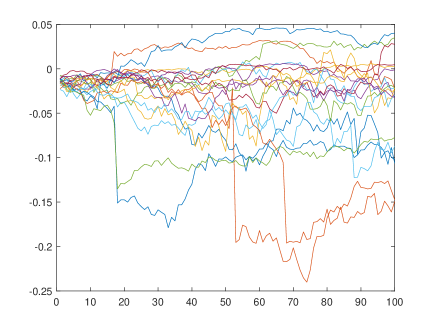
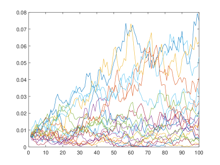
Figure 1: CGMYSV sample paths (left) and CIR sample paths (right).

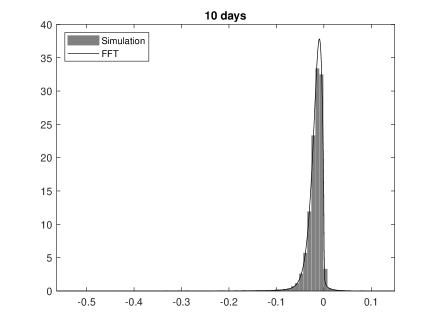
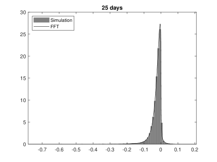
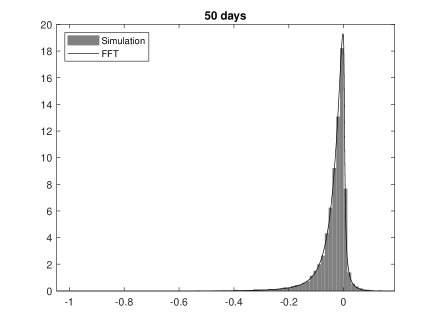
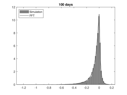
Figure 2: CGMYSV pdfs based on the simulated sample path (gray bar-plots) vs pdf using FFT method (solid curves). Distributions of $X_{t}$ are for $t=10\varDelta t$ (top-left), $t=25\varDelta t$ (top-right), $t=50\varDelta t$ (bottom-left), and $t=10\varDelta t$ (bottom-right), where $\varDelta t=1/252$ is one day of year fraction.

In order to verify the performance of Algorithm 1, we generate a set of example sample paths of the CGMYSV process $\{L_{t}\}_{t\geq 0}$ with parameters $\alpha=0.52$, $\lambda_{+}=25.46$, $\lambda_{-}=4.604$, $\kappa=1.003$, $\eta=0.0711$, $\zeta=0.3443$, $v_{0}=0.0064$, and $\rho=-2.0280$. We set $M=100$, $J=1024$, $N=10,000$ , and ${\varDelta t}=1/252$ which is the annual fraction of 1 day. Example 20 sample-paths are presented in the first plate of Figure 1. The second plate of the figure is for 20 sample path of CIR process. For goodness of fit test for the generated path, we perform Kolmogorov-Smirnov test. We compare the distribution of 10-days simulated random numbers $\{L_{n,10}|n=1,2,\cdots,N\}$ with the distribution of $L_{10{\varDelta t}}$. The cumulative distribution function of $L_{10{\varDelta t}}$ can be obtained by the Ch.F of the CGMYSV using the inverse Fourier-Transform methos (See Carr et al. (2002) and Rachev et al. (2011) more details). Table 1 presents the result of the KS test, and it has 70.29% $p$-value and it is not rejected at the 5% significant level. Using the same arguments, we perform KS test for 25-days, 50-days, and 100-days simulated random numbers. They are not rejected at the 5% significant level, either. We graphically compare the empirical probability density function (pdf) of the simulated sample path and the CGMYSV pdfs for those four cases. We draw empirical pdfs using gray bar charts and draw solid lines for CGMYSV pdfs in four plates in Figure 2.

4 The CGMYSV Option Pricing Model

In this section we discuss the option pricing model on the CGMYSV model. We define the model and calibrate parameters using European style S&P 500 index option (SPX option) and American style S&P 100 index option (OEX option).

Let $r$ and $q$ be the risk free rate of return and the continuous dividend rate of a given underlying asset, respectively. The risk-neutral price process $\{S_{t}\}_{t\geq 0}$ of a given underlying asset is assumed as

$$S_{t}=\frac{S_{0}\exp((r-q)t+L_{t})}{E\left[\exp(L_{t})\right]}$$ (8)

where $\{L_{t}\}_{t\geq 0}$ is the CGMYSV process with parameters $(\alpha$, $\lambda_{+}$, $\lambda_{-}$, $\kappa$, $\eta$, $\zeta$, $\rho$, $v_{0})$. By (5), we also have

$$S_{t}=\frac{S_{0}\exp((r-q)t+L_{t})}{\Phi_{t}(-i\log\phi_{stdCTS}(-i;\alpha,\lambda_{+},\lambda_{-}),-\rho i,v_{0})}.$$

4.1 Calibration to European Options

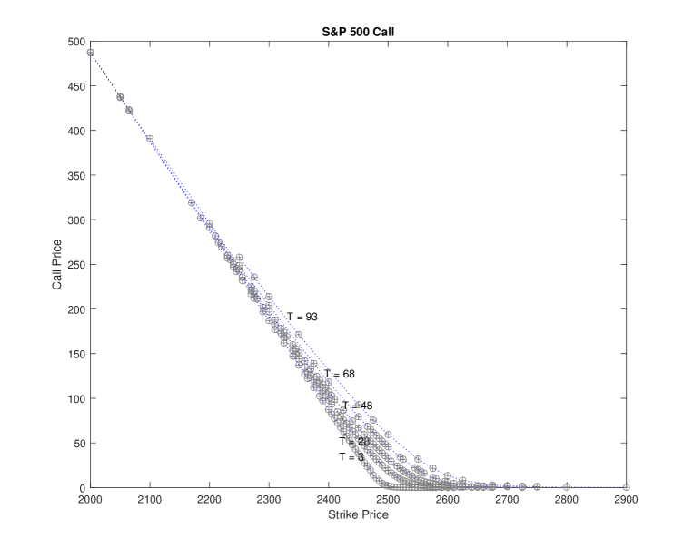
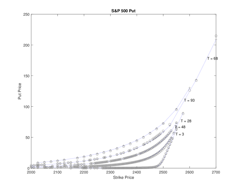
Figure 3: Observed SPX option price and model prices calibrated to the market prices for Call (top) and put (bottom) on September 11, 2017. ‘$\circ$’ stands for the market price and ‘+’ stands for the FFT price.

On the risk neutral price process $\{S_{t}\}_{t\geq 0}$ defined by (8), the European call and put prices with the strike price $K$ and the time to maturity $T$ are equal to $C(K,T)=e^{-rT}E[(S_{t}-K)^{+}]$ and $C(K,T)=e^{-rT}E[(K-S_{t})^{+}]$, respectively. Moreover, the Fast-Fourier-Transform (FFT) method by Carr and Madan (1999) and Boyarchenko and Levendorskiĭ (2000), we can calculate European call/put prices numerically. We calibrate the CGMYSV parameters $(\alpha$, $\lambda_{+}$, $\lambda_{-}$, $\kappa$, $\eta$, $\zeta$, $\rho$, $v_{0})$ using the SPX option prices on September 11, 2017. We observed 247 call prices and 289 put prices on the day. The S&P 500 price $S_{0}$, risk-free rate of return, and continuous dividend rate at the day were $S_{0}=2488.11$, $r=1.213\%$, and $q=1.884\%$ respectively. The calibration results for SPX calls and puts are provided in Table 2. Figure 3 shows observed SPX call and put prices ( drawn by ‘$\circ$’), and calibrated CGMYSV prices using FFT (drawn by ‘$+$’).

We recalculate the European call and put prices using Monte-Carlo Simulation (MCS) method with the calibrated parameters in Table 2. The sample paths of the MCS method are generated by Algorithm 1. The number of sample paths is 10,000 in this investigation.

To compare the MCS method with the FFT method, we use the four error estimators:the average absolute error (AAE), the average absolute error as a percentage of the mean price (APE), the average relative percentage error (ARPE), and the root mean square error (RMSE) (see Schoutens (2003)). Those four error estimators for the FFT method and the MCS method are in Table 3. Both call and put cases, the MCS method has larger error estimators than the FFT method. That is not surprising because we calibrate those parameters using the FFT method. The table says that the four error estimators of MCS method are similar to those of the FFT method. That means the sample path generation with Algorithm 1 performs well, and prices by the MCS are similar performance as FFT method.

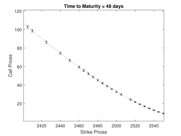
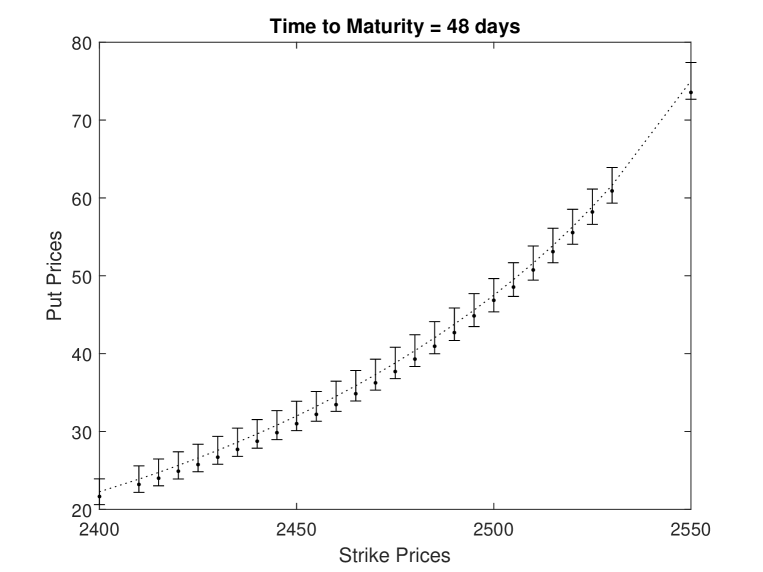
Figure 4: Confidence Intervals for the MCS option prices. Dots are observed market prices, dot-coves are MCS prices, and ‘I’ shape bars are 95% confidence intervals of MCS prices. The first (top) plate is for call option pricing and the second (bottom) plate is for put option pricing.

In this option pricing with MCS method, we also obtain standard error for each 247 call and 289 put options, but we do not provide them all because of the space limitation. Instead, we show MCS prices with the 95% confidence interval in Figure 4 only for the case $2,400<K<2,600$ and time to maturity 48 days.

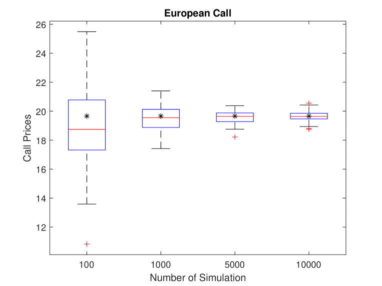
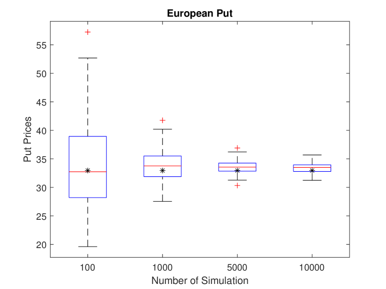
Figure 5: Boot strapping for call (top) and put (bottom).

Finally, we perform the bootstrapping. We select an at-the-money call and an at-the-money put of $K=2,500$ and $T=28\,days$ as an example, and calculate call and put prices with MCS parameters in Table 2, respectively. Table 4 shows that the MCS prices and their standard errors for 100, 1,000, 5,000, and 10,000 number of sample paths. We repeat this process 100 times and draw boxplots. Boxplots for call and put for each number of sample paths are the up plate and the bottom plate of Figure 5. Stars in those boxplots are the call/put prices using FFT method. We can observe that the number of sample paths increases, then the MCS prices close to the FFT price and dispersions are reduced.

4.2 Calibration to American Options

We see that the sample path generation method using the series representation works for MCS of European option pricing in the previous section. In this section, we discuss the American option pricing with the same sample path generation method. We use Least Square Regression Method (LSM) by Longstaff and Schwartz (2001) for American option pricing with MCS. When we do the regression for the expected value of option, we use $S_{t}$, $S_{t}^{2}$, $\sigma_{t}$, $\sigma_{t}^{2}$ and $\sigma_{t}S_{t}$ as independent variables, following the idea in Chapter 15 of Rachev et al. (2011).

For empirical illustration, we use market prices of the OEX option, which is American style. We calibrate parameters of the CGMYSV model with fixed seed numbers for each random number generation. That is, we fix a seed number of $\chi^{2}$ random number generator in the CIR process, and we generate uniform and exponential random numbers $U_{j}$, $U^{\prime}_{j}$, $E_{j}$, $E^{\prime}_{j}$ and $\tau_{j}$ with predefined seed numbers, and fix them. Then we set the model parameters, generate sample paths using Algorithm 1 with the fixed seed number and the fixed random number sets, and then calculate American option price using LSM. Repeat that process and find the optimal parameters to minimize RMSE. As a benchmark, we calibrate the parameters of the CGMY option pricing model (See Carr et al. (2002)) to the OEX option prices using LSM with sample path generated by the series representation explained in Section 2.3.

The calibration results are presented in Table 5. We calibrate the CGMY and the CGMYSV model parameters for 12 Wednesdays in 2015 and 2016 exhibited in the table. The four error estimators, AAE, APE, ARPE, and RMSE, are also provided in Table 6. Since the smaller error estimator means the better calibration performance, smaller errors are written in bold letters for each day. This table shows that the CGMYSV calibration performs better than CGMY calibration except for the cases of February 10, 2016 and June 10, 2015. On March 9, 2016, AAE and APE of the CGMY model are less than those of CGMYSV, but ARPE and RMSE of CGMY are larger than those of CGMYSV. ARPE of CGMY is smaller than that of CGMYSV on November 10, 2015, but the other three error values of CGMY are larger than CGMYSV. Therefore, we can conclude that the CGMYSV option pricing model performs typically better than the CGMY option pricing model, except in a few cases in this investigation. Hence, LSM with Algorithm 1 works well in the American option calibration.

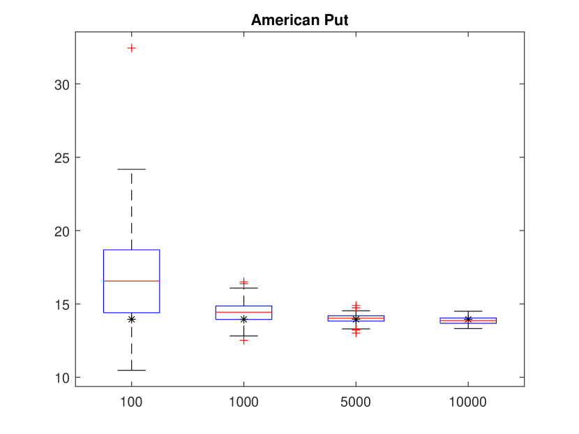
Figure 6: Boot strapping for OEX put option with time to maturity of $T=31days$ and strike price $K=910$.

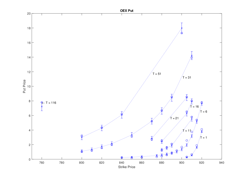
Figure 7: OEX put prices on April 6, 2016 and LSM prices with their confidence intervals. Circles (‘$\circ$’) are observed OEX put prices, ‘$\times$’ points are MCS prices, and ‘I’ shape bars are 95% confidence intervals of LMS prices.

Finally, we perform the bootstrapping. We selected the at-the-money put for the strike price $K=910$ and the days to maturity $T=31$ days on April 6, 2016. Put prices are obtained by LSM using parameters calibrated to the day provided in Table 5. On the day, the underlying S&P 100 index price was 918.21, and the market put price was 13.95 for the strike price 910 and 31 days to maturity. Table 7 shows that the LSM prices and their standard errors for 100, 1,000, 5,000, and 10,000 number of sample paths. The LSM prices approach to the market price and the standard error decreases as the number of sample paths increases. We repeat this process 100 times and present boxplots for those 100 prices, as Figure 6. Stars in those boxplots are the market put prices. We can observe that the LSM prices close to the market price and dispersions are reduced as the number of sample paths increases. Additionally, Figure 7 provides a graphical illustration of the calibration for April 6, 2016. Calibrated CGMYSV prices are drawn by ‘$\times$’, the market observed prices are drawn by ‘$\circ$’, and the 95% confidence intervals are marked by ’I’ shape. The day to maturities $T$ are written on the plate.

4.3 Asian and Barrier options

The sample path generation method for the CGMYSV model can be used for Asian and Barrier option pricing. In this section, we briefly show examples of Asian and Barrier option pricing using MCS with the sample path generated by Algorithm 1.

We generate 10,000 sample path of the CGMYSV model with parameters $\alpha=0.52$, $\lambda_{+}=25.46$, $\lambda_{-}=4.604$, $\kappa=1.003$, $\eta=0.0711$, $\zeta=0.3443$, $v_{0}=0.0064$, and $\rho=-2.0280$. Then we generate the underlying price process $\{S_{t}\}_{t\geq 0}$ using (8) where $S_{0}=2,488$, $r=0.0121$, $d=0.0188$.

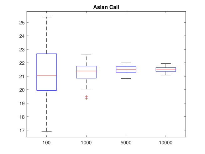
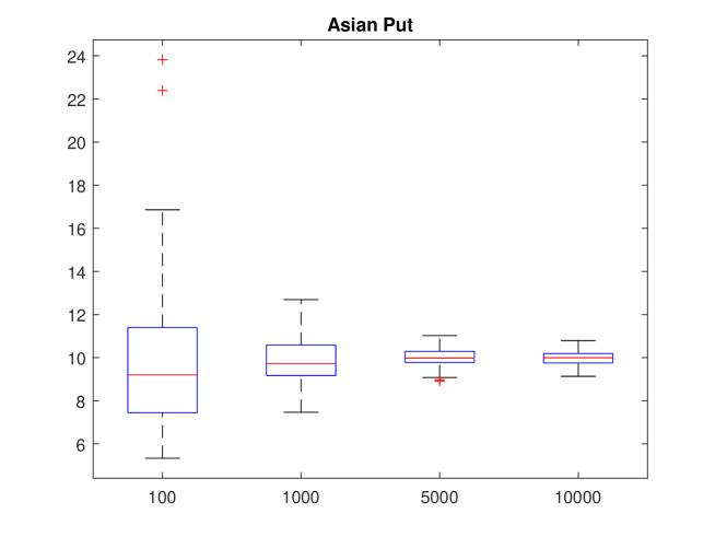
Figure 8: Boot strapping for Asian call (top) & put (bottom).

For the Asian option, we consider the arithmetic average call and put where the strike price $K=2,500$ and the time to maturity $T=25days$. Table 8 shows that the MCS prices for Asian call & put and their standard errors for 100, 1,000, 5,000, and 10,000 number of sample paths. The the standard error of the MCS prices decreases as the number of sample paths increases. We repeat this process 100 times and present boxplots for those 100 prices, as Figure 8. We can observe that the MCS prices converge, and dispersions are reduced as the sample paths increase.

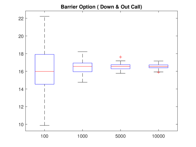
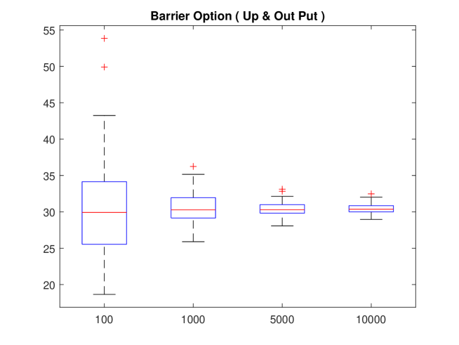
Figure 9: Boot strapping for Barrier options: the down-and-out call (top) and the up-and-out put (bottom).

With the same argument, we find MCS price for the Barrier options. We consider the down-and-out call and the up-and-out put Barrier options with the strike price $K=2,500$ and the time to maturity $T=25days$. Barrier of the down-and-out call and the up-and-out put are $2,400$ and $2,750$, respectively. Table 9 shows that the MCS prices and their standard errors for 100, 1,000, 5,000, and 10,000 number of sample paths. The standard error of the MCS prices decreases as the number of sample paths increases. We repeat this process 100 times and present boxplots for those 100 prices, as Figure 9. We can also observe that the MCS prices converge, and dispersions are reduced as the sample paths increase.

5 Conclusion

In this paper, we develop the CGMYSV sample path generation algorithm using the series representation. The series representation method’s performance is tested by comparing the simulated distribution to the pdf calculated by the inverse Fourier transform method. We apply the sample path generation method to European and American option pricing with MCS and LSM. We compare the MCS method to the FFT method in European option pricing with SPX option market data. Also, we calibrate the parameters of the CGMYSV model to the American style OEX option using LSM. We measure the performance of the calibration using four error estimators and the boot-strapping method. We conclude that the sample path generation method of CGMYSV model performs well, and it can be successfully applied to American option pricing with LSM. Finally, we present Asian and Barrier option pricing examples with MCS method using the sample path generation algorithm.

Acknowledgments The author is grateful to Professor Svetlozar T. Rachev for his valuable discussion on this problem and encouragement. The author gratefully acknowledges the support of GlimmAnalytics LLC and Juro Instruments Co., Ltd.

	KS statistic	$p$-value
10 days	0.0070	0.7029
25 days	0.0122	0.1026
50 days	0.0069	0.7296
100 days	0.0110	0.1748

Table 1: KS test for distributions of simulated sample paths

Parameter	Call	Put
$\alpha$	$0.5184$	$0.0089$
$\lambda_{+}$	$25.4592$	$2.0852$
$\lambda_{-}$	$4.6040$	$6.2380$
$\kappa$	$1.0029$	$1.4333$
$\eta$	$0.0711$	$0.1961$
$\zeta$	$0.3443$	$1.1931$
$\rho$	$-2.0283$	$-0.1695$
$v_{0}$	$0.006381$	$0.0619$

Table 2: Calibrated Parameters for the SPX option at September 11, 2017.

	Call			Put
Error	FFT	MCS		FFT	MCS
AAE	$0.4442$	$0.6220$		$0.4047$	$0.5512$
APE	$0.0053$	$0.0074$		$0.0226$	$0.0308$
ARPE	$0.0711$	$0.0813$		$0.2094$	$0.1672$
RMSE	$0.6016$	$0.8019$		$0.7006$	$0.8608$

Table 3: Error estimators for the parameter calibration to the call and put option market price at September 11, 2017.

	Call			Put
Number of Simulation	Price	Standard error		Price	Standard error
100	15.9651	2.1001		34.3371	7.9356
1000	17.8790	0.7511		32.5601	2.2353
5000	19.6536	0.3634		32.7791	1.0458
10000	19.6840	0.2551		32.6914	0.7617
FFT Price	19.6590			32.9541
Market Price	19.05			31.50

Table 4: MCS prices and standard errors for SPX call and put with the strike price $K=2500$ and time to maturity $T=28\,days$ using calibrated parameters at September 11, 2017.

	CGMY					CGMYSV
Date	$\alpha$	$C$	$\lambda_{+}$	$\lambda_{-}$		$\alpha$	$\lambda_{+}$	$\lambda_{-}$	$\kappa$	$\eta$	$\zeta$	$v_{0}$	$\rho$
Apr. 6, 2016	$0.5459$	$0.3495$	$6.3595$	$7.7563$		$1.1356$	$35.2115$	$7.7883$	$1.9322$	$0.3550$	$1.2211$	$0.0100$	$1.2237$
Mar. 9, 2016	$1.6885$	$0.0246$	$21.2919$	$2.8805$		$0.0353$	$20.3911$	$9.9256$	$2.1262$	$0.4570$	$1.2665$	$0.0236$	$1.3434$
Feb. 10, 2016	$0.9287$	$3.5284$	$72.5855$	$46.4594$		$0.0257$	$1.3491$	$0.7503$	$2.4301$	$0.4185$	$1.8126$	$0.2711$	$0.3567$
Jan. 6, 20166	$1.2290$	$0.4104$	$64.6344$	$21.3096$		$1.3081$	$33.2233$	$32.5605$	$2.0656$	$0.4237$	$1.8947$	$0.0810$	$0.1172$
Dec. 9, 2015	$1.3241$	$0.2984$	$57.6574$	$30.2749$		$0.6308$	$40.5190$	$24.3874$	$5.0247$	$0.3299$	$3.5989$	$0.0593$	$0.2334$
Nov. 10, 2015	$1.5907$	$0.0184$	$26.4398$	$2.7714$		$0.0266$	$1.6365$	$0.7506$	$1.0354$	$0.5658$	$0.3936$	$0.1111$	$1.2914$
Oct. 7, 2015	$0.9792$	$0.2955$	$53.8624$	$8.4758$		$0.8763$	$65.0630$	$67.4571$	$1.8555$	$0.2794$	$2.1050$	$0.0422$	$0.0080$
Sep. 9, 2015	$1.2572$	$0.5862$	$54.0807$	$15.3905$		$0.5836$	$30.2731$	$17.2115$	$5.1193$	$0.3569$	$4.8231$	$0.1189$	$0.1158$
Aug. 12, 2015	$0.7574$	$0.5926$	$61.7876$	$14.2761$		$0.4848$	$42.9235$	$31.7027$	$2.1644$	$0.1964$	$2.1032$	$0.0283$	$0.1639$
Jul. 8, 2015	$1.1742$	$0.2429$	$78.6224$	$11.4198$		$0.9127$	$46.3671$	$46.3013$	$2.2125$	$0.2173$	$2.0394$	$0.0547$	$-0.0637$
Jun. 10, 2015	$1.3849$	$0.0407$	$64.9276$	$7.8355$		$0.0391$	$1.0381$	$0.7820$	$1.1451$	$0.6167$	$0.6062$	$0.0518$	$1.2736$
May. 6, 2015	$1.2247$	$0.1125$	$87.0744$	$8.6069$		$0.8628$	$53.8182$	$54.3726$	$2.0949$	$0.2023$	$2.0731$	$0.0352$	$0.0647$

Table 5: Parameter Calibration Results for the OEX Option market

Date	Model	AAE	APE	ARPE	RMSE
Apr. 6, 2016	CGMY	0.6623	0.1726	0.4587	0.8833
	CGMYSV	0.1881	0.0490	0.1242	0.2497
Mar. 9, 2016	CGMY	0.6780	0.1106	0.2871	0.8323
	CGMYSV	0.6833	0.1115	0.2492	0.8086
Feb. 10, 2016	CGMY	0.7755	0.0513	0.1282	1.1076
	CGMYSV	0.9267	0.0613	0.2075	1.2042
Jan. 6, 2016	CGMY	0.6945	0.0644	0.1617	0.9379
	CGMYSV	0.4140	0.0384	0.0784	0.6574
Dec. 9, 2015	CGMY	0.7986	0.0931	0.1855	1.1230
	CGMYSV	0.5903	0.0688	0.0957	0.7885
Nov. 10, 2015	CGMY	0.3137	0.0576	0.2169	0.4159
	CGMYSV	0.2337	0.0429	0.2560	0.3815
Oct. 7, 2015	CGMY	0.5268	0.1018	0.3741	0.6891
	CGMYSV	0.2186	0.0423	0.1520	0.3221
Sep. 9, 2015	CGMY	0.8948	0.0880	0.1681	1.2499
	CGMYSV	0.5874	0.0577	0.1002	0.9153
Aug. 12, 2015	CGMY	0.6464	0.0941	0.1894	0.9097
	CGMYSV	0.4137	0.0602	0.1401	0.5652
Jul. 8, 2015	CGMY	0.7636	0.0800	0.1456	1.0079
	CGMYSV	0.2518	0.0264	0.1023	0.3238
Jun. 10, 2015	CGMY	0.2535	0.0671	0.2576	0.3483
	CGMYSV	0.3180	0.0841	0.3676	0.4120
May. 6, 2015	CGMY	0.7361	0.0765	0.1479	0.9776
	CGMYSV	0.3880	0.0403	0.1097	0.5137

Table 6: Error Estimates for the calibration of the OEX option

	Put
Number of Simulation	Price	Standard error
100	15.4565	2.7280
1000	15.0373	1.0173
5000	13.9616	0.3990
10000	13.8768	0.2856
Market Price	13.950

Table 7: MCS prices and standard errors for the OEX put with time to maturity of $T=31days$ and strike price $K=910$ using parameters calibrated at April 6, 2016.

	Call			Put
Number of Simulation	Price	Standard error		Price	Standard error
100	22.0834	1.7485		11.7400	3.4463
1000	21.0078	0.5866		9.7009	1.0759
5000	21.4664	0.2785		10.5634	0.5443
10000	21.6513	0.1937		9.9964	0.3679

Table 8: MCS prices and standard errors for Asian call & put.

	Down & Out Call			Up & Out Put
Number of Simulation	Price	Standard error		Price	Standard error
100	12.9019	1.4535		36.2543	3.6254
1000	15.3738	0.5165		30.0687	0.9509
5000	16.6097	0.2460		31.8030	0.4498
10000	16.5518	0.1749		30.2590	0.3026

Table 9: MCS prices and standard errors for the down-and-out call and the up-and-out put.

References

- Bianchi et al. (2010) Bianchi, M. L., Rachev, S. T., Kim, Y. S., and Fabozzi, F. J. (2010). Tempered infinitely divisible distributions and processes. Theory of Probability and Its Applications (TVP), Society for Industrial and Applied Mathematics (SIAM), 55(1), 58–86.
- Black and Scholes (1973) Black, F. and Scholes, M. (1973). The pricing of options and corporate liabilities. The Journal of Political Economy, 81(3), 637–654.
- Boyarchenko and Levendorskiĭ (2000) Boyarchenko, S. I. and Levendorskiĭ, S. Z. (2000). Option pricing for truncated Lévy processes. International Journal of Theoretical and Applied Finance, 3, 549–552.
- Carr et al. (2002) Carr, P., Geman, H., Madan, D., and Yor, M. (2002). The fine structure of asset returns: An empirical investigation. Journal of Business, 75(2), 305–332.
- Carr et al. (2003) Carr, P., Geman, H., Madan, D., and Yor, M. (2003). Stochastic volatility for Lévy processes. Mathematical Finance, 13, 345–382.
- Carr and Madan (1999) Carr, P. and Madan, D. (1999). Option valuation using the fast fourier transform. Journal of Computational Finance, 2(4), 61–73.
- Cox et al. (1985) Cox, J., Ingersoll, J., and Ross, S. (1985). A theory of the term structure of interest rates. Econometrica, 53, 385–407.
- Heston (1993) Heston, S. (1993). A closed-form solution for options with stochastic volatility with applications to bond and currency options. Review of Financial Studies, 6, 327–343.
- Kim et al. (2011) Kim, S., Rachev, S. T., Bianchi, M. L., Mitov, I., and Fabozzi, F. J. (2011). Time series analysis for financial market meltdowns. Journal of Banking and Finance, 35, 1879–1891.
- Kim et al. (2010) Kim, Y. S., Rachev, S. T., Bianchi, M. L., and Fabozzi, F. J. (2010). Tempered stable and tempered infinitely divisible GARCH models. Journal of Banking and Finance, 34, 2096–2109.
- Koponen (1995) Koponen, I. (1995). Analytic approach to the problem of convergence of truncated Lévy flights towards the gaussian stochastic process. Physical Review E, 52, 1197–1199.
- Lamberton and Lapeyre (1996) Lamberton, D. and Lapeyre, B. (1996). Introduction to Stochastic Calculus Applied Finaice. Chapman & Hall/CRC.
- Longstaff and Schwartz (2001) Longstaff, F. A. and Schwartz, E. S. (2001). Valuing American options by simulation: a simple least-squares approach. Review of Financial Studies, 14, 113–148.
- Rachev et al. (2011) Rachev, S. T., Kim, Y. S., Bianch, M. L., and Fabozzi, F. J. (2011). Financial Models with Lévy Processes and Volatility Clustering. John Wiley & Sons.
- Rachev and Mittnik (2000) Rachev, S. T. and Mittnik, S. (2000). Stable Paretian Models in Finance. John Wiley & Sons: New York.
- Rosiński (2007) Rosiński, J. (2007). Tempering stable processes. Stochastic Processes and Their Applications, 117(6), 677–707.
- Schoutens (2003) Schoutens, W. (2003). Lévy Processes in Finance: Pricing Financial Derivatives. John Wiley and Sons: Chichester.