Hubs-biased resistance distances on graphs and networks

Abstract

We define and study two new kinds of “effective resistances” based on hubs-biased – hubs-repelling and hubs-attracting – models of navigating a graph/network. We prove that these effective resistances are squared Euclidean distances between the vertices of a graph. They can be expressed in terms of the Moore–Penrose pseudoinverse of the hubs-biased Laplacian matrices of the graph. We define the analogous of the Kirchhoff indices of the graph based of these resistance distances. We prove several results for the new resistance distances and the Kirchhoff indices based on spectral properties of the corresponding Laplacians. After an intensive computational search we conjecture that the Kirchhoff index based on the hubs-repelling resistance distance is not smaller than that based on the standard resistance distance, and that the last is not smaller than the one based on the hubs-attracting resistance distance. We also observe that in real-world brain and neural systems the efficiency of standard random walk processes is as high as that of hubs-attracting schemes. On the contrary, infrastructures and modular software networks seem to be designed to be navigated by using their hubs.

AMS Subject Classification: 05C50; 05C82; 15A18; 47N50

1 Introduction

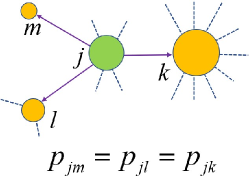
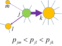
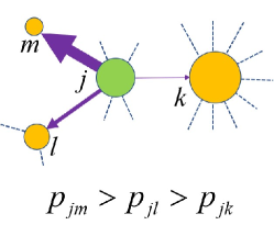
Random walk and diffusive models are ubiquitous in mathematics, physics, biology and social sciences, in particular when the random walker moves through the vertices and edges of a graph $G=\left(V,E\right)$ [35, 1, 12, 8, 36]. In this scenario a random walker at the vertex $j\in V$ of $G$ at time $t$ can move to any of the nearest neighbors of $j$ with equal probability at time $t+1$ [35]. That is, if as illustrated in Fig. 1.1(a) the vertex $j$ has three nearest neighbors $\left\{k,l,m\right\}$ the random walker can move to any of them with probability $p_{jm}=p_{jl}=p_{jk}=k_{j}^{-1}$, where $k_{j}$ is the degree of $j$. We can figure out situations in which the movement of the random walker at a given position is facilitated by the large degree of any of its nearest neighbors. Here we use a relaxed definition of the term “hub”. Although this term is used in network theory for those nodes of exceptionally large degree, we use it here in the following way: If there are two connected vertices of different degree, we call a “hub” the one of larger degree. This is formally defined later on in the paper.

Then, let us suppose that there are situations in which the probability that the random walker moves to a nearest neighbor of $j$ at time $t+1$ increases with the degree of the nearest neighbor. This is illustrated in Fig. 1.1(b) where $k_{i}>k_{l}>k_{m}$, and consequently $p_{jm}<p_{jl}<p_{j{i}}$. We will refer hereafter to this scenario as the “hubs-attracting” one. Another possibility is that the random walker is repelled by large degree vertices, such as for $k_{i}>k_{l}>k_{m}$, we have $p_{jm}>p_{jl}>p_{j{i}}$ as illustrated in Fig. 1.1(c). We will refer to this model as the “hubs-repelling” one. These scenarios could be relevant in the context of real-world complex networks where vertices represent the entities of the system and the edges the interrelation between them [4, 42, 19]. An example of hubs-repelling strategies of navigation are some of the diffusive processes in the brain where there is a high energetic cost for navigating through the hubs of the system [47, 46]. Hubs-attracting mechanisms could be exhibited, for instance, by diffusive epidemic processes in which hubs are major attractors of the disease and can be considered at high risk of contagion by spreaders in the network [41].

(a)

(b)

(c)

Figure 1.1: Schematic illustration of a normal (a), hubs-attracting (b) and hubs-repelling schemes of a particle hopping on a network.

From a mathematical perspective, one of the most important aspects of the model of random walks on graphs is its connection with the graph Laplacian matrix [37, 38, 29, 30, 45] and with the concept of resistance distance [17, 34, 43, 48, 28, 18]. In a simple graph the resistance distance is the effective resistance between two vertices $v$ and $w$, which measures the resistance of the total system when a voltage is connected across $v$ and $w$. Klein and Randić [34] proved that the effective resistance is a squared Euclidean distance between the two vertices of the graph, which can be obtained from the Moore–Penrose pseudoinverse of the graph Laplacian. It is also known that the commute time between two vertices $v$ and $w$ of a random walker [17, 43, 28, 18], i.e., the number of steps of a random walker starting at $v$, before arriving at $w$ and returning to $v$ again, is proportional to the resistance distance between the two vertices.

Strategies for avoiding large/small degree vertices in random-walk processes on graphs/networks have been proposed in the literature under the general umbrella of ‘degree-biased random walks’ [9, 39, 27, 6]. However, in the current work we go beyond the random walk formulation of the problem and express it in terms of hubs-biased Laplacians [22, 26] and the corresponding resistance distance matrices on graphs. Thus, we focus here on the algebraic properties of these resistance distance matrices. We note in passing that the current concept has nothing in common with the so-called “degree-resistance” between a pair of vertices, which is nothing else that the resistance distance multiplied by the difference of degrees of the vertices forming the corresponding edge [31].

Due to the relation between resistance distance and commute time of random walks on graphs, we study here the efficiency of hubs attracting/repelling diffusive processes on graphs. In closing, in this work we define the hubs-biased resistance distances between pairs of vertices of a simple graph and study their main spectral properties. We also propose analogues of the Kirchhoff index [34, 50, 44, 14], the semi-sum of all resistance distances in the graph, for the hubs-biased resistances. We report here several bounds for the two new kinds of resistance distances as well as for the corresponding Kirchhoff indices. Finally, we study the commute time of the hubs-attracting random walks and analyze their relative improvement over the standard one. We observe that certain classes of real-world networks, such as brain/neuronal networks and electronic circuits, have normal random walks as efficient as the hubs-attracting one, while others, like infrastructural networks, can reduce their average commuting times by 300% by using the hubs-attracting mechanism.

2 Preliminaries

In this article we consider simple weighted graphs. We will always impose the following throughout.

Assumptions 2.1.

$G$ is a weighted graph with vertex set $V$ and edge set $E$. The underlying unweighted graph $(V,E)$ is simple and finite: we denote by $n,m\in\mathbb{N}$ the number of vertices and edges, respectively. To avoid trivialities, we also assume $n\geq 2$ and that no vertex is isolated. We also denote by $\mathcal{C}$ its number of connected components.

Additionally, each edge is assigned a weight by means of a surjective mapping $\varphi:E\rightarrow W$, with $W\subset(0,\infty)$.

In the following we use interchangeably the terms graphs and networks.

Let $A$ be the adjacency matrix of the (weighted) graph $G$ and let $k_{i}$ denote the degree of the vertex $i\in V$, i.e., the sum of the $i$th row or column of $A$; or equivalently $k_{i}:=\#\mathcal{N_{\mathit{i}}}$ where $\mathcal{N_{\mathit{j}}}=\left\{j\in V|\left(i,j\right)\in E\right\}$ is the set of all nearest neighbors of $i$. We will denote the minimal and maximum degree by $\delta$ and $\varDelta$, respectively. Let $j$ be a node such that $j\in{\mathcal{N_{\mathit{i}}}}$. Then, we say that $j$ is a “hub”, more correctly a “local hub”, if it has the largest degree among all $j\in{\mathcal{N_{\mathit{i}}}}$. We will denote by $K$ the diagonal matrix of vertex degrees.

We use the following condensed notation across this paper. If $x_{\alpha}$ is a number depending on an index $\alpha$ – in the following typically $\alpha\in\left\{-1,1\right\}$ – then we will write $x_{\alpha}$ to symbolize both $x_{-1}$ and $x_{1}$ depending on the choice on the index $\alpha$. Let $\ell^{2}(V)$ be the finite-dimensional Hilbert space of functions on $V$ with respect to the inner product

$$\langle f,g\rangle=\sum_{v\in V}f(v)\overline{g(v)},\qquad f,g\in\ell^{2}(V).$$

The standard graph Laplacian is an operator in $\ell^{2}(V)$ which is defined by

$$\bigl{(}\mathscr{L}f\bigr{)}(v)\coloneqq\sum_{w\in V:\,(v,w)\in E}{\varphi(vw)}\bigl{(}f(v)-f(w)\bigr{)},\qquad f\in\ell^{2}(V),$$ (2.1)

where $\varphi(v,w)\in W$ is the weight of the edge $(v,w)\in E$.

Finally, in the following ${1_{n}}$ will denote the all-ones column vector of order $n$; $J_{n}$ the $n\times n$ all-one matrix; and $I_{n}$ the identity matrix of order $n$.

3 Hubs-biased Laplacians and their spectra

Here we introduce the concepts of hubs-biased Laplacians in the context of resistive networks.

Definition 3.1.

A conductance function is a function $c:V\times V\rightarrow\mathbb{R}^{+}$ which respects adjacency between vertices, i.e., $\left(v,w\right)\in E$ if and only if $c\left(v,w\right)>0$.

Definition 3.2.

The total conductance at a vertex $v$ is defined as

$$\begin{split}c\left(v\right)&\coloneqq\sum_{\left(v,w\right)\in E}c\left(v,w\right)\\ &=\sum_{w\in V}c\left(v,w\right).\end{split}$$ (3.1)

(The second equality in (3.1) holds in view of Definition 3.1.)

To motivate the following definition, let us now consider a diffusive particle that does not necessarily hop to any nearest neighbor with the same probability. More precisely, in a hubs-attracting model the hopping of a diffusive particle from a vertex $i$ to a target neighboring vertex $j$ is favored by a (comparatively) small degree of $i$ and a large degree of $j$ (“$j$ is a hub”), corresponding to a small ratio $\frac{k_{i}}{k_{j}}$. On the other hand, the hopping from $i$ to $j$ is disfavored by a (comparatively) large degree of $i$ and a (comparatively) small degree of $j$. Notice that these conditions for the hopping from $i$ to $j$ are different from the ones for the hopping from $j$ to $i$: hubs-attracting diffusion is not symmetric.

Specularly, hubs-repelling models are conceivable in which the hopping from $i$ to $j$ would be favored by a comparatively large degree of $i$ and a comparatively small degree of $j$, and disfavored by a comparatively small degree of $i$ and a comparatively large degree of $j$.

We will capture this intuition by the following.

Definition 3.3.

Let $G$ be a graph satisfying the Assumptions 2.1 and let $\alpha\in\left\{-1,1\right\}.$ The hubs-biased Laplacian corresponding to $\alpha$ is the operator on $\ell^{2}(V)$ defined by

$$\bigl{(}\mathscr{L}_{\alpha}f\bigr{)}(v)\coloneqq\sum_{w\in\mathcal{N}_{v}}c_{\alpha}\left(v,w\right)\bigl{(}f(v)-f(w)\bigr{)},\qquad f\in\ell^{2}(V),$$ (3.2)

where here and in the following

$$c_{\alpha}\left(v,w\right):=\left(\dfrac{k_{v}}{k_{w}}\right)^{\alpha}.$$ (3.3)

We call $\mathscr{L}_{\alpha}$ the hubs-repelling Laplacian if $\alpha=1$ and hence $c_{\alpha}\left(v,w\right)=\dfrac{k_{v}}{k_{w}}$; or hubs-attracting Laplacian if $\alpha=-1$ and hence $c_{\alpha}\left(v,w\right)=\dfrac{k_{w}}{k_{v}}$.

Remark 3.4.

Actually, we could easily extend this definition by allowing for any $\alpha\in{\mathbb{R}}$; for $\alpha=0$, corresponding to the unweighted case, we would then recover the standard (discrete) Laplacian ${\mathscr{L}}_{0}$. However, we will not explore this direction in this paper.

Remark 3.5.

In order to understand the main difference between the current approach and some previous approaches introduced for the analysis of weighted directed graphs we should point out the following. First, we analyze here unweighted and undirected graphs, which are then transformed into a very specific kind of weighted directed graphs. In [5, 49, 3, 7], among others, the authors focus on weighted directed graphs. Then, they generate either asymmetric Laplacians $L^{a}$ [5, 3] or symmetrized versions $L^{s}$ thereof [5, 7]. Yet another approach was proposed by Young et al. [49] where the resistance distances are calculated from a matrix $X=2Q^{T}{\Sigma}Q$ where $\tilde{\mathscr{L}}{\Sigma}+{\Sigma}\tilde{\mathscr{L}}^{T}=I_{n-1}$, $\tilde{\mathscr{L}}=QLQ^{T}$ and the matrix $Q$ obeys the following conditions: $Q1_{n}=0$, $QQ^{T}=I_{n-1}$ and $Q^{T}Q=I_{n}-(1/n)J_{n}$. The matrix $\tilde{\mathscr{L}}=Q{\mathscr{L}}Q^{T}$ is known as the reduced Laplacian. In a further work, Fitch [25] demonstrated that the resistance distances obtained through the matrix $X$ for any pair of vertices in any connected, directed graph, are equal to the resistance distances obtained for a certain symmetric, undirected Laplacian on the same set of nodes and possibly admitting negative edge weights. As the hubs-biased Laplacian matrices are non-symmetric in general, it is obvious that these two approaches are not equivalent.

In the current study a different kind of matricial structure emerges, which is neither the asymmetric cases previously considered nor a symmetric one. The matrices $\mathscr{L}_{\alpha}$ correspond to the class of quasi-reciprocal matrices (see [32]), which has not been previously used in the analysis of graphs. An $n\times n$ matrix $M$ is called quasi-reciprocal if

$$M_{ij}\neq 0\Rightarrow M_{ji}=M_{ij}^{-1},\forall i,j=1,2,\ldots,n.$$ (3.4)

Therefore, due to this notable difference the approach developed here for the resistance distance and related descriptions of undirected graphs are substantially different from the ones previously analyzed for weighted directed graphs [5, 49, 3, 7].

Let $e_{v}$, $v\in V$ be a standard orthonormal basis in $\ell^{2}(V)$ consisting of the vectors

$$e_{v}(w)\coloneqq\begin{cases}1&\text{if $w=v$},\\[2.15277pt] 0&\text{otherwise}.\end{cases}$$ (3.5)

Then, $\mathscr{L}_{\alpha}$ acts on the vectors $e_{v}$ as follows:

$$(\mathscr{L}_{\alpha}e_{v})(w)=\begin{cases}c_{\alpha}(v)&\text{if $w=v$},\\[2.15277pt] -c_{\alpha}\left(v,w\right)&\text{if $(v,w)\in E$},\\[2.15277pt] 0&\text{otherwise},\end{cases}$$ (3.6)

where

$$c_{\alpha}(v)=\sum_{w\in\mathscr{\mathcal{N_{\mathit{v}}}}}c_{\alpha}\left(v,w\right)$$ (3.7)

is the total $\alpha$-conductance of the vertex $v$. Then, the hubs-biased matrices can be expressed as

$$\mathscr{L}_{\alpha}=\Xi_{\alpha}-K^{\alpha}AK^{-\alpha},$$ (3.8)

where

$$\begin{split}\Xi_{\alpha}&:=\operatorname{diag}\left(c_{\alpha}(v)\right)_{v\in V},\\ K&:=\operatorname{diag}\left(k_{v}\right)_{v\in V},\end{split}$$ (3.9)

and $A$ is the unweighted adjacency matrix of the graph.

Let us note an elementary but important fact concerning the trace of (any) hubs-biased Laplacians.

Lemma 3.6.

There holds

$$\operatorname{tr_{{}_{\,HB}}}\left(G\right):=\textnormal{tr}\left(\mathscr{L}_{1}\right)=\textnormal{tr}\left(\mathscr{L}_{-1}\right)=\sum_{v,w\in V}a_{vw}\dfrac{k_{v}}{k_{w}}.$$ (3.10)

Proof.

Let us, for $\alpha\in\{-1,1\}$, consider the definition of total conductance and in view of (3.1),

$$\textnormal{tr}\left(\mathscr{L}_{\alpha}\right)=\sum_{v\in V}c_{\alpha}\left(v\right)=\sum_{v,w\in V}a_{vw}\left(\dfrac{k_{v}}{k_{w}}\right)^{\alpha}.$$ (3.11)

Now, because $a_{v,w}=1$ if and only if $a_{w,v}=1$ (and in this case both addends $\dfrac{k_{v}}{k_{w}},\dfrac{k_{w}}{k_{v}}$ appear), we conclude that

$$\textnormal{tr}\left(\mathscr{L}_{\alpha}\right)=\sum_{v\in V}c_{\alpha}\left(v\right)=\sum_{v,w\in V}a_{vw}\dfrac{k_{v}}{k_{w}}:$$ (3.12)

since the right-hand side is independent of $\alpha$, the claim is proved. ∎

Remark 3.7.

A rather natural generalization of Definition 3.3 involves infinite graphs. Let for a moment – unlike under the standing Assumptions 2.1! – the graph $G$ be allowed to have infinitely many vertices. If the degree sequence $(k_{v})_{v\in V}$ is still bounded, then by (3.3) and (3.7) the sequence $(c_{\alpha}(v))_{v\in V}$ is bounded, too; it is then easy to see that the matrices $\Xi_{\alpha}$, $K^{\pm\alpha}$, and $A$ define bounded linear operators on the (infinite dimensional!) space $\ell^{2}(V)$. We conclude that for such infinite, uniformly locally bounded graphs $\mathcal{L}_{\alpha}$ is well-defined as a bounded linear operator on $\ell^{2}(V)$, too. However, $A$ and hence $\mathcal{L}_{\alpha}$ have absolutely continuous spectrum, rather than a discrete set of eigenvalues as in the finite case: for this reason, this setting is not convenient for our purposes: for example, $\mathcal{L}_{\alpha}$ will not have finite trace.

The double-sided bound

$$2m\dfrac{\delta}{\varDelta}\leq\operatorname{tr_{{}_{\,HB}}}\left(G\right)\leq 2m\dfrac{\varDelta}{\delta}$$ (3.13)

on the hubs-biased trace immediately follows from (3.10), since $\delta\leq k_{v}\leq\varDelta$ for all $v\in V$, and because $\sum_{v,w\in V}a_{vw}=\sum_{v\in V}k_{v}=2m$ by the Handshaking Lemma. (We recall that $\delta$ and $\varDelta$ denote the minimum and maximum degree of the vertices of $G$, respectively, and $m$ is the number of edges of $G$.)

The estimates in (3.13) are rough, yet sharp as both inequalities become equalities for complete graphs. (We should observe that if $G$ is complete, then $\operatorname{tr_{{}_{\,HB}}}\left(G\right)$ also agrees with the trace of the standard discrete Laplacian.)

We are able to provide a few improved estimates.

Lemma 3.8.

There holds

$$\dfrac{1}{\varDelta}\sum_{v\in V}k_{v}^{2}\leq\operatorname{tr_{{}_{\,HB}}}\left(G\right)\leq\dfrac{1}{\delta}\sum_{v\in V}k_{v}^{2}.$$ (3.14)

Proof.

The bounds follow directly from (3.10), since

$$\sum_{w\in V}a_{vw}k_{v}=k_{v}\sum_{w\in V}a_{vw}=k_{v}^{2}\qquad\hbox{for all $v\in V$}.$$ (3.15)

Summing over $v\in V$ yields the claimed bounds. ∎

Because of the well-known identity

$$\sum_{v\in V}k_{v}^{2}=\sum_{(v,w)\in E}\left(k_{v}+k_{w}\right),$$

the estimates in (3.14) imply those in (3.13), but are clearly sharper if, e.g., $G$ is bi-regular (recall that $G$ is bi-regular if $V$ can be partitioned in $V_{1},V_{2}$ with $k_{v}\equiv k_{1}\in\mathbb{N}$ for all $v\in V_{1}$; and $k_{w}\equiv k_{2}\in\mathbb{N}$ for all $w\in V_{2}$).

More explicit bounds in (3.14) can be obtained using known estimates on $\sum_{v\in V}k_{v}^{2}$ and $\sum_{v\in V}k_{v}^{-1}$, the so-called (first) Zagreb index and Randić index of $G$, respectively: we refer to [2] for a comprehensive survey of results on this topic, including improving bounds for special classes, like planar or triangle-free graphs, that might be of interest in applications. In particular, we mention the following.

Corollary 3.9.

There holds

$$\dfrac{4m^{2}}{n\varDelta}\leq\operatorname{tr_{{}_{\,HB}}}\left(G\right)\leq\dfrac{2m\left(2m+\left(n-1\right)\left(\varDelta-\delta\right)\right)}{\delta\left(n+\varDelta-\delta\right)}.$$ (3.16)

The lower estimate becomes an equality if and only if $G$ is regular. The upper estimate becomes an equality if and only if $G$ is a graph with $t$ vertices of degree $n-1$ and the remaining $n-t$ vertices forming an independent set.

Proof.

The claimed bounds follow from the known estimates

$$\dfrac{4m^{2}}{n}\leq\sum_{v\in V}k_{v}^{2}\leq\dfrac{2m\left(2m+\left(n-1\right)\left(\varDelta-\delta\right)\right)}{n+\varDelta-\delta}:$$ (3.17)

cf. [11, Remark 4 and Remark 5] and [13], where also the extremal graphs are characterized. ∎

Remark 3.10.

(1) The lower estimate in (3.16) is significantly better than the lower estimate in (3.13): indeed, the net effect is like replacing $\delta$ by the average degree $\dfrac{2m}{n}$ in (3.13). The upper estimate in (3.16) is better than the upper estimate in (3.13) if and only if

$$2m+\left(n-1\right)\left(\varDelta-\delta\right)\leq\varDelta\left(n+\varDelta-\delta\right),$$ (3.18)

which is sometimes the case, for instance for any regular graph, and sometimes not, for instance for any path on more than 2 edges. The equality in (3.18) holds for complete graphs.

(2) Further estimates on the hubs-biased trace may be obtained re-writing (3.10) in alternative ways, including

$$\sum_{v,w\in V}a_{vw}\dfrac{k_{v}}{k_{w}}=\sum_{v\in V}k_{v}\left(\sum_{w\in V}\dfrac{a_{vw}}{k_{w}}\right)=\sum_{v\in V}k_{v}\left(\sum_{w\in\mathcal{N}_{v}}\dfrac{1}{k_{w}}\right),$$ (3.19)

or

$$\sum_{v,w\in V}a_{vw}\dfrac{k_{v}}{k_{w}}=\sum_{v\in V}\dfrac{1}{k_{v}}\left(\sum_{w\in V}a_{vw}k_{w}\right)=\sum_{v\in V}\dfrac{1}{k_{v}}\left(\sum_{w\in\mathcal{N}_{v}}k_{w}\right)$$ (3.20)

(we recall that $\mathcal{N}_{v}$ is the set of nearest neighbors of $v$). Considering the minima $\delta_{\mathcal{N}_{v}}$ and maxima $\varDelta_{\mathcal{N}_{v}}$ of the degree function in neighborhoods $\mathcal{N}_{v}$ we can deduce from (3.19) and (3.20) the following sharper estimates:

$$\sum_{v\in V}\dfrac{k_{v}^{2}}{\varDelta_{\mathcal{N}_{v}}}\leq\operatorname{tr_{{}_{\,HB}}}\left(G\right)\leq\sum_{v\in V}\dfrac{k_{v}^{2}}{\delta_{\mathcal{N}_{v}}},$$ (3.21)

$$\sum_{v\in V}\delta_{\mathcal{N}_{v}}\leq\operatorname{tr_{{}_{\,HB}}}\left(G\right)\leq\sum_{v\in V}\varDelta_{\mathcal{N}_{v}},$$ (3.22)

which shows, for instance, that $\operatorname{tr_{{}_{\,HB}}}\left(G\right)=2pq$ for the complete bipartite graph $K_{p,q}.$

(3) Invoking Titu’s Lemma we also obtain

$$\sum_{w\in\mathcal{N}_{v}}\dfrac{1}{k_{w}}\geq\dfrac{\left(\sum_{w\in\mathcal{N}_{v}}1\right)^{2}}{\sum_{w\in\mathcal{N}_{v}}k_{w}}=\dfrac{k_{v}^{2}}{\sum_{w\in\mathcal{N}_{v}}k_{w}}.$$ (3.23)

Because Titu’s Lemma is equivalent to the Cauchy–Schwarz inequality, the previous inequality becomes an equality if and only if $\left(1\right)_{w\in\mathcal{N}_{v}}$ and $\left(k_{w}\right)_{w\in\mathcal{N}_{v}}$ are linearly dependent, i.e., if and only if the degree function is constant on each neighborhood, which is the case for instance in regular and bi-regular graphs. We finally deduce the estimate

$$\operatorname{tr_{{}_{\,HB}}}\left(G\right)\geq\sum_{v\in V}\dfrac{k_{v}^{3}}{\sum_{w\in\mathcal{N}_{v}}k_{w}},$$ (3.24)

which of course implies the lower estimate in (3.21).

Let us now collect a few important properties of the hubs-biased Laplacian matrices of any graphs satisfying our standing Assumptions 2.1.

Theorem 3.11.

Let $\alpha\in\{-1,1\}$. Then the hubs-biased Laplacian matrix ${\mathscr{L}}_{\alpha}$ enjoys the following properties:

(i) its eigenvalues are real;

(ii) it is positive semidefinite;

(iii) $\textnormal{{rank\,}}{\mathscr{L}}_{\alpha}=n-\mathscr{C}$;

(iv) it can be diagonalized as ${\mathscr{L}}_{\alpha}=\left(KU_{\alpha}\right)\Lambda_{\alpha}\left(KU_{\alpha}\right)^{-1}$, where $\Xi_{\alpha}-A=U_{\alpha}\Lambda_{\alpha}U_{\alpha}^{-1}$ and $K$ is as in (3.9).

Proof.

(i) Under the Assumptions 2.1, no vertex is isolated, hence $k_{i}\geq 1$ for all $i$. Therefore, for any $\alpha\in\left\{-1,1\right\}$ the diagonal matrix $K^{\alpha}$ is invertible and we observe that

$$\begin{split}{\mathscr{L}}_{\alpha}&=\Xi_{\alpha}-K^{\alpha}AK^{-\alpha}\\ &=K^{\alpha}\left(K^{-\alpha}\Xi_{\alpha}K^{\alpha}-A\right)K^{-\alpha}\\ &=K^{\alpha}\left(\Xi_{\alpha}-A\right)K^{-\alpha},\end{split}$$ (3.25)

since $\Xi_{\alpha}$ is diagonal, too. We conclude that ${\mathscr{L}}_{\alpha}$ is similar to the symmetric matrix $\left(\Xi_{\alpha}-A\right)$, and so their eigenvalues are real.

(ii) Now let $x\in\ell^{2}(V)$ and $x\neq{0}$. Then, we can write

$$\begin{split}x^{T}\left(\Xi_{\alpha}-A\right)x&=\sum_{\left(i,j\right)\in E}\left(\left(k_{i}^{\alpha/2}k_{j}^{-\alpha/2}\right)x_{i}-\left(k_{j}^{\alpha/2}k_{i}^{-\alpha/2}\right)x_{j}\right)^{2}\end{split}\geq 0.$$ (3.26)

Therefore, because $\Xi_{\alpha}-A$ and ${\mathscr{L}}_{\alpha}$ are similar, we have that ${x}^{T}{\mathscr{L}}_{\alpha}{x}\geq 0$.

(iii) Let us now prove that the dimension of the null space of ${\mathscr{L}}_{\alpha}$ is $\mathscr{C}$. Let ${z}$ be a vector such that ${\mathscr{L}}_{\alpha}{z}=0$. This implies that for every $\left(i,j\right)\in E$, $z_{i}=z_{j}$. Therefore ${z}$ takes the same value on all vertices of the same connected component, which indicates that the dimension of the null space is $\mathscr{C}$, and so $\textnormal{{rank\,}}{\mathscr{L}}_{\alpha}=n-\mathscr{C}$.

(iv) Finally, we also have that because $\Xi_{\alpha}-A$ is symmetric we can write it as: $\Xi_{\alpha}-A=U_{\alpha}\Lambda_{\alpha}U_{\alpha}^{-1}$. Thus, ${\mathscr{L}}_{\alpha}=\left(KU_{\alpha}\right)\Lambda_{\alpha}\left(KU_{\alpha}\right)^{-1}$ which indicates that all hubs-biased Laplacians are diagonalizable. ∎

We know from Theorem 3.11 that all eigenvalues of any hubs-biased Laplacian are real positive: we will denote them by $\rho_{\alpha,1}\ldots,\rho_{\alpha_{n}}$ in ascending order, i.e.,

$$0=\rho_{\alpha,1}\leq\ldots\leq\rho_{\alpha,n}.$$

Let us conclude this section deducing some estimates on them. To avoid trivialities, and in view of Theorem 3.11.(iii), in the remainder of this section we always assume the graph $G$ to be connected.

Corollary 3.12.

Let $\alpha\in\left\{-1,1\right\}$. Then we have

$$\rho_{\alpha,n}\geq\frac{4m^{2}}{n(n-1)\varDelta}$$ (3.27)

and

$$\left.\begin{array}[]{c}\dfrac{2m\left(2m+\left(n-1\right)\left(\varDelta-\delta\right)\right)}{\delta(n-1)\left(n+\varDelta-\delta\right)}\\[15.0pt] \dfrac{2m\varDelta}{(n-1)\delta}\end{array}\right\}\geq\rho_{\alpha,2}.$$ (3.28)

We note in passing that on a $\left(k+1\right)$-star, the upper bounds in (3.28) reduce to

$$\left.\begin{array}[]{c}2+k\\ 2k+1\end{array}\right\}\geq\rho_{\alpha,2,}$$ (3.29)

which does not prevent $\rho_{\alpha,2}$ to tend to $+\infty$ as the graph grows.

We also remark that these estimates are only really interesting for non-regular graphs, because in regular graphs the hubs-biased Laplacians coincide with the standard discrete Laplacian for which many different bounds are known for its eigenvalues.

Proof.

Observe that $\dfrac{1}{n-1}\operatorname{tr_{{}_{\,HB}}}\left(G\right)$ yields the arithmetic mean of all non-zero eigenvalues of ${\mathscr{L}}_{\alpha}$; in particular, the lowest non-zero eigenvalue $\rho_{\alpha,2}$ cannot be larger than $\dfrac{1}{n-1}\operatorname{tr_{{}_{\,HB}}}\left(G\right)$ while the largest eigenvalue $\rho_{\alpha,n}$ cannot be larger that $\dfrac{1}{n-1}\operatorname{tr_{{}_{\,HB}}}\left(G\right)$. Taking into account (3.13) and (3.16) we deduce the claimed estimate. ∎

Remark 3.13.

(1) The naive upper bound

$$\rho_{\alpha,n}\leq 2\max_{v\in V}\left({\mathscr{L}}_{\alpha}\right)_{vv}$$ (3.30)

on the largest eigenvalue of ${\mathscr{L}}_{\alpha}$ follows from Geršgorin’s Theorem, since by (3.6) $\left({\mathscr{L}}_{\alpha}\right)_{vv}=\sum_{w\in V}\left|\left({\mathscr{L}}_{\alpha}\right)_{vw}\right|$. Now,

$$\begin{split}\left({\mathscr{L}}_{-1}\right)_{vv}&=\sum_{w\in\mathcal{N}_{v}}\dfrac{k_{w}}{k_{v}}\leq\dfrac{\varDelta_{\mathcal{N}_{v}}}{k_{v}}\sum_{w\in\mathcal{N}_{v}}1=\varDelta_{\mathcal{N}_{v}}\leq\varDelta,\\ \left({\mathscr{L}}_{1}\right)_{vv}&=\sum_{w\in\mathcal{N}_{v}}\dfrac{k_{v}}{k_{w}}\leq\dfrac{k_{v}}{\delta}\sum_{w\in\mathcal{N}_{v}}1=\dfrac{k_{v}^{2}}{\delta}\leq\dfrac{\varDelta^{2}}{\delta},\end{split}$$ (3.31)

which are both sharp for regular graphs. Plugging these expressions in (3.30) yields

$$\rho_{-1,n}\leq 2\varDelta$$ (3.32)

and

$$\rho_{1,n}\leq 2\dfrac{\varDelta^{2}}{\delta}.$$ (3.33)

(2) In order to show some lower bounds on $\rho_{\alpha,2}$, we remark that the standard discrete Laplacian $\mathcal{\mathscr{L}}$ and ${\mathscr{L}}_{\alpha}$ share the null space, cf. the proof of Theorem 3.11.(iii). Then, we can quotient it out, thus studying the lowest eigenvalue of $\mathcal{\mathscr{L}}$ and ${\mathscr{L}}_{\alpha}$ on $\mathbb{C}^{n}/\left\langle{\mathbf{1}}\right\rangle$, the space of vectors orthogonal to the vector ${\mathbf{1}}=(1,\ldots,1)$. Taking a normalized vector $f$ in this space one sees that

$$\dfrac{\delta}{\varDelta}\left(\mathscr{L}f,f\right)\leq\left(\mathscr{L}_{\alpha}f,f\right).$$ (3.34)

In particular, choosing $f$ to be an eigenfunction associated with the lowest non-zero eigenvalue $\rho_{\alpha,2}$ of $\mathscr{L}_{\alpha}$ and applying the Courant–Fischer min-max characterization of the eigenvalues of the Hermitian matrix we deduce

$$\dfrac{\delta}{\varDelta}\rho_{2}\leq\rho_{\alpha,2},$$ (3.35)

where $\rho_{2}$ is the second lowest eigenvalue of the discrete Laplacian, i.e., the algebraic connectivity [16]. Alternatively, for $\alpha=-1$ we can use

$$\delta\left(\mathscr{L}_{\textnormal{norm}}f,f\right)\leq\left(\mathscr{L}_{\alpha}f,f\right),$$ (3.36)

and deduce

$$\delta\rho_{2,\textnormal{norm}}\leq\rho_{\alpha,2},$$ (3.37)

where $\mathscr{L}_{\textnormal{norm}}\coloneqq K^{-1/2}\mathscr{L}K^{-1/2}$ is the normalized Laplacian. Now we can either apply explicit formulae for $\rho_{2}$ and $\rho_{2,\textnormal{norm}}$ for classes of graphs or use general estimates like

$$\rho_{2}\geq 2\eta\left(1-\cos\dfrac{\pi}{n}\right),$$ (3.38)

from [23] or

$$\rho_{2,\textnormal{norm}}\geq\left\{\begin{array}[]{c}\dfrac{1}{Dn},\\ 1-\cos\dfrac{\pi}{m},\end{array}\right.$$ (3.39)

from [10, 33], respectively, where $\eta\geq 1$ is the edge connectivity and $D$ is the diameter of $G$.

(3) Further sharp bounds on the Zagreb index are known, including [15, Theorem 2.3 and Theorem 2.6], immediately yielding

$$\varDelta+\frac{(2m-\varDelta)^{2}}{\varDelta(n-1)}+\frac{2(n-2)(\varDelta_{2}-\delta)^{2}}{\varDelta(n-1)^{2}}\leq\operatorname{tr_{{}_{\,HB}}}(G)\leq\frac{(n+1)m-\varDelta(n-\varDelta)}{\delta}+\frac{2(m-\varDelta)^{2}}{\delta(n-2)},$$

where $\varDelta_{2}$ denotes the second largest degree of $G$, the upper bound holding under the additional assumption that $n\geq 3$. (A characterization of the extremal graphs where equality is attained is available, too, but is rather technical.)

Following the same proof as in Corollary 3.12 finally yields the bounds

$$\rho_{\alpha,n}\geq\frac{\varDelta}{n-1}+\frac{(2m-\varDelta)^{2}}{\varDelta(n-1)^{2}}+\frac{2(n-2)(\varDelta_{2}-\delta)^{2}}{\varDelta(n-1)^{3}}$$

and

$$\frac{(n+1)m-\varDelta(n-\varDelta)}{\delta(n-1)}+\frac{2(m-\varDelta)^{2}}{\delta(n-2)(n-1)}\geq\rho_{\alpha,2}.$$

4 Hubs-biased Resistance Distance

We adapt here some general definitions of resistive networks to the case of hubs-biased systems, mainly following the classic formulations given in [17, 34, 18]. Let us consider $G$ as a resistive network in which every edge $\left(v,w\right)\in E$ has edge resistance $r_{\alpha}\left(v,w\right)\coloneqq c_{\alpha}^{-1}\left(v,w\right)$.

Let us consider the connection of a voltage between the vertices $v$ and $w$, and let $i\left(v,w\right)>0$ be the net current out the source $v$ and into the sink $w$, such that $i\left(v,w\right)=-i\left(w,v\right).$ Then, according to the first Kirchhoff’s law we have that $\sum_{w\in\mathcal{N}_{v}}i\left(v,w\right)=I$ if $v$ is a source, $\sum_{w\in\mathcal{N}_{v}}i\left(v,w\right)=-I$ if $v$ is a sink, or zero otherwise, where we have denoted by $I$ the net current flowing through the whole network. The application of the second Kirchhoff’s law, namely that $\sum_{\left(v,w\right)\in C}i\left(v,w\right)r_{\alpha}\left(v,w\right)=0$ where $C$ is a cycle with edges labeled in consecutive order, implies that a potential $\mathscr{V}$ may be associated with any vertex $v$, such that for all edges

$$i\left(v,w\right)r_{\alpha}\left(v,w\right)=\mathscr{V}\left(v\right)-\mathscr{V}\left(w\right),$$ (4.1)

which represents the Ohm’s law, and where $i$ and $\mathscr{V}$ depend on the net current $I$ and on the pair of vertices where the voltage source has been placed. Let us now define formally the hubs-biased effective resistance, which is the resistance of the total system when a voltage source is connected across a corresponding pair of vertices. Throughout this section we are still adopting the notation in Section 3: in particular, $\alpha\in\{-1,1\}$.

Definition 4.1.

The hubs-biased effective resistance between the vertices $v$ and $w$ of $G$ is

$$\Omega_{\alpha}\left(v,w\right):=\dfrac{\mathscr{V}\left(v\right)-\mathscr{V}\left(w\right)}{I}.$$ (4.2)

We now prove the following result, showing that hubs-biased resistance between any two vertices of $G$ is a squared Euclidean distance.

Lemma 4.2.

Let $v,w\in V$. Then for $\alpha\in\{-1,1\}$ the hubs-biased resistance $\Omega_{\alpha}\left(v,w\right)$ is given by

$$\Omega_{\alpha}\left(v,w\right)=\mathscr{L}_{\alpha}^{+}\left(v,v\right)+\mathscr{L}_{\alpha}^{+}\left(w,w\right)-\mathscr{L}_{\alpha}^{+}\left(v,w\right)-\mathscr{L}_{\alpha}^{+}\left(w,v\right),$$ (4.3)

where $\mathscr{L}_{\alpha}^{+}$ stands for the Moore–Penrose pseudoinverse of $\mathscr{L}_{\alpha}$.

Proof.

First, we will prove that

$$\Omega_{\alpha}\left(v,w\right)=\left({e}_{v}-{e}_{w}\right)^{T}\mathscr{L}_{\alpha}^{+}\left(v,v\right)\left({e}_{v}-{e}_{w}\right),$$ (4.4)

where ${e}_{v}$ is the vector with all entries equal to zero except the one corresponding to vertex $v$ which is equal to one. Using the second Kirchhoff’s law we have

$$\sum_{w\in\mathcal{N}_{v}}\dfrac{1}{r\left(v,w\right)}\left(\mathscr{V}\left(v\right)-\mathscr{V}\left(w\right)\right)=\begin{cases}I\qquad&\hbox{if $v$ is a source},\\ -I\qquad&\hbox{if $v$ is a sink},\\ 0&\hbox{otherwise},\end{cases}$$ (4.5)

which can also be written as

$$c_{\alpha}\left(v\right)\mathscr{V}\left(v\right)-\sum_{w=1}^{n}\dfrac{1}{r\left(v,w\right)}\mathscr{V}\left(w\right)=\begin{cases}I\qquad&\hbox{if $v$ is a source},\\ -I\qquad&\hbox{if $v$ is a sink},\\ 0&\hbox{otherwise}.\end{cases}$$ (4.6)

Let us write it in matrix-vector form as

$$\mathscr{\mathscr{L}_{\alpha}{V}}=I\left({e}_{v}-{e}_{w}\right).$$ (4.7)

Due to the fact that the right-hand side of (4.7) is orthogonal to ${1}$ we can obtain ${\mathscr{V}}$ as

$$\mathscr{V}\left(v\right)-\mathscr{V}\left(w\right)=\left({e}_{v}-{e}_{w}\right)^{T}\mathscr{{V}}=I\left({e}_{v}-{e}_{w}\right)^{T}\mathscr{L}_{\alpha}^{+}\left({e}_{v}-{e}_{w}\right).$$ (4.8)

Then, using the definition of the effective resistance we have

$$\Omega_{\alpha}\left(v,w\right)=\dfrac{\mathscr{V}\left(v\right)-\mathscr{V}\left(w\right)}{I}=\left({e}_{v}-{e}_{w}\right)^{T}\mathscr{L}_{\alpha}^{+}\left({e}_{v}-{e}_{w}\right).$$ (4.9)

Now, because $\left({e}_{v}-{e}_{w}\right)^{T}\mathscr{L}_{\alpha}^{+}\left({e}_{v}-{e}_{w}\right)=\mathscr{L}_{\alpha}^{+}\left(v,v\right)+\mathscr{L}_{\alpha}^{+}\left(w,w\right)-\mathscr{L}_{\alpha}^{+}\left(v,w\right)-\mathscr{L}_{\alpha}^{+}\left(w,v\right)$ we only remain to prove that it is a distance. Let $\mathscr{L}_{\alpha}=V_{\alpha}\Lambda_{\alpha}V_{\alpha}^{-1}$, where $V_{\alpha}=KU_{\alpha}.$ Then $\mathscr{L}_{\alpha}^{+}=V_{\alpha}\Lambda_{\alpha}^{+}V_{\alpha}^{-1},$ with $\Lambda_{\alpha}^{+}$ being the Moore–Penrose pseudoinverse of the diagonal matrix of eigenvalues of$\mathscr{L}_{\alpha},$ i.e., the diagonal matrix whose $i$th entry is

$$\Lambda_{\alpha}^{+}\left(i,i\right)=\begin{cases}0\quad&\hbox{if the $i$th eigenvalue is $0$},\\ \rho_{\alpha,i}^{-1}\quad&\hbox{if the $i$th eigenvalue is $\neq 0$}.\end{cases}$$

Let us write the right-hand side of (4.3) as

$${v}_{\alpha}\Lambda_{\alpha}^{+}{u}_{\alpha}^{T}+{w}_{\alpha}\Lambda_{\alpha}^{+}{w}_{\alpha}^{T}-{v}_{\alpha}\Lambda_{\alpha}^{+}{w}_{\alpha}^{T}-{w}_{\alpha}\Lambda_{\alpha}^{+}{v}_{\alpha}^{T},$$ (4.10)

where ${v}$ and ${w}$ are the corresponding rows of $V_{\alpha}$ for the vertices $u$ and $w$, respectively. Then, we have

$$\begin{split}&\mathscr{L}_{\alpha}^{+}\left(u,u\right)+\mathscr{L}_{\alpha}^{+}\left(w,w\right)-\mathscr{L}_{\alpha}^{+}\left(u,w\right)-\mathscr{L}_{\alpha}^{+}\left(w,u\right)\\ &={v}_{\alpha}\left(\Lambda_{\alpha}^{+}{v}_{\alpha}^{T}-\Lambda_{\alpha}^{+}{w}_{\alpha}^{T}\right)-{w}_{\alpha}\left(\Lambda_{\alpha}^{+}{v}_{\alpha}^{T}-\Lambda_{\alpha}^{+}{w}_{\alpha}^{T}\right),\\ &=\left({v}_{\alpha}-{w}_{\alpha}\right)\left(\Lambda_{\alpha}^{+}{v}_{\alpha}^{T}-\Lambda_{\alpha}^{+}{w}_{\alpha}^{T}\right)\\ &=\left({v}_{\alpha}-{w}_{\alpha}\right)\Lambda_{\alpha}^{+}\left({v}_{\alpha}-{w}_{\alpha}\right)^{T}\\ &=\left(\left({v}_{\alpha}-{w}_{\alpha}\right)\sqrt{\Lambda_{\alpha}^{+}}\right)\left(\left({v}_{\alpha}-{w}_{\alpha}\right)\sqrt{\Lambda_{\alpha}^{+}}\right)^{T}\\ &=\left(\mathscr{V}_{\alpha}\left(v\right)-\mathscr{V}_{\alpha}\left(w\right)\right)^{T}\left(\mathscr{V}_{\alpha}\left(v\right)-\mathscr{V}_{\alpha}\left(w\right)\right)\\ &=\left\|\mathscr{V}_{\alpha}\left(v\right)-\mathscr{V}_{\alpha}\left(w\right)\right\|^{2},\end{split}$$ (4.11)

where $\mathscr{V}_{\alpha}\left(v\right)={v}_{\alpha}\sqrt{\Lambda_{\alpha}^{+}}$ is the position vector of the vertex $v$ in the Euclidean space induced by the hubs-repelling Laplacian. ∎

Corollary 4.3.

Let $\alpha\in\{-1,1\}$ and $\mathscr{L}_{\alpha}=V_{\alpha}\Lambda_{\alpha}V_{\alpha}^{-1}$, where $V_{\alpha}:=KU_{\alpha}$ for $V_{\alpha}:=\left[{\psi}_{\alpha,1},{\psi}_{\alpha,2},\cdots,{\psi}_{\alpha n}\right]$ and $\Lambda_{\alpha}:=\operatorname{diag}\left(\rho_{\alpha,k}\right)$. Then,

$$\Omega_{\alpha}\left(u,w\right)=\sum_{k=2}^{n}\rho_{\alpha,k}^{-1}\left(\psi_{\alpha,k,u}-\psi_{\alpha,k,w}\right)^{2}.$$ (4.12)

Proof.

It is easy to see from Lemma 4.2 that

$$\begin{split}\Omega_{\alpha}\left(u,w\right)&=\sum_{k=2}^{n}\rho_{\alpha,k}^{-1}\psi_{\alpha,k,u}^{2}+\sum_{k=2}^{n}\rho_{\alpha,k}^{-1}\psi_{\alpha,k,w}^{2}-2\sum_{k=2}^{n}\rho_{\alpha,k}^{-1}\psi_{\alpha,k,u}\psi_{\alpha,k,w}\\ &=\sum_{k=2}^{n}\rho_{\alpha,k}^{-1}\left(\psi_{\alpha,k,u}^{2}+\psi_{\alpha,k,w}^{2}-2\psi_{\alpha,k,u}\psi_{\left\{R,A\right\},k,w}\right)\\ &=\sum_{k=2}^{n}\rho_{\alpha,k}^{-1}\left(\psi_{\alpha,k,u}-\psi_{\alpha,k,w}\right)^{2}.\end{split}$$ (4.13)

∎

Corollary 4.4.

Let $\alpha=\{-1,1\}$ and $0=\rho_{\alpha,1}<\rho_{\alpha,2}\leq\cdots\leq\rho_{\alpha,n}$ be the eigenvalues of $\mathscr{L}_{\alpha}$. Then,

$$\dfrac{2}{\rho_{\alpha,n}}\leq\Omega_{\alpha}\left(u,w\right)\leq\dfrac{2}{\rho_{\alpha,2}}.$$ (4.14)

Proof.

Using Corollary 4.3 and the fact that $\rho_{\alpha,2}$ is the smallest eigenvalue of $\mathscr{L}_{\alpha}$ we have the upper bound if all the eigenvalues are equal to $\rho_{\alpha,2}$. The result follows from the fact that $\sum_{k=1}^{n}\psi_{\alpha,k,u}^{2}=1$ and $\sum_{k=1}^{n}\psi_{\alpha,k,u}\psi_{\alpha,k,w}=0$ for every $u\neq w$. The lower bound is obtained similarly by the fact that $\rho_{\alpha,n}$ is the largest eigenvalue of $\mathscr{L}_{\alpha}$. ∎

4.1 Hubs-biased Kirchhoff index

In full analogy with the definition of the so-called Kirchhoff index by Klein and Randić [34] we define here the hubs-biased Kirchhoff indices of a graph.

Definition 4.5.

Let $\alpha\in\{-1,1\}$. The total hubs-biased resistance distance, or hubs-biased Kirchhoff index, of a graph $G$ is defined as

$$\mathcal{\mathscr{R}}_{\alpha}\left(G\right)=\sum_{v<w}\Omega_{\alpha}\left(v,w\right).$$ (4.15)

Lemma 4.6.

Let $\alpha\in\{-1,1\}$ and $0=\rho_{\alpha,1}<\rho_{\alpha,2}\leq\cdots\leq\rho_{\alpha,n}$ be the eigenvalues of $\mathscr{L}_{\alpha}$. Then,

$$\mathcal{\mathscr{R}}_{\alpha}\left(G\right)=n\sum_{k=2}^{n}\dfrac{1}{\rho_{\alpha,k}}.$$ (4.16)

Proof.

Let us write the sum of the hubs-biased resistance distances as

$$\begin{split}\dfrac{1}{2}\sum_{v,w\in V}\Omega_{\alpha}\left(u,w\right)&=\dfrac{1}{2}\left({1}^{T}\textnormal{diag$\left(\mathscr{L}_{\alpha\ }^{+}\right){1}^{T}$}{1}+{1}^{T}{1}\left(\operatorname{diag}\left(\mathscr{L}_{\alpha}^{+}\right)\right)^{T}{1}-{1}^{T}\mathscr{L}_{\alpha}^{+}{1}-{1}^{T}\left(\mathscr{L}_{\alpha}^{+}\right)^{T}{1}\right)\\ &=\dfrac{1}{2}\left(2n\textnormal{tr}\left(\mathscr{L}_{\alpha}^{+}\right)\right)\\ &=n\sum_{k=2}^{n}\dfrac{1}{\rho_{\alpha,k}},\end{split}$$

where $\textnormal{tr}\left(\mathscr{L}_{\alpha}^{+}\right)$ is the trace of $\mathscr{L}_{\alpha}^{+}$. ∎

Corollary 4.7.

Let $\alpha\in\{-1,1\}$ and $0=\rho_{\alpha,1}<\rho_{\alpha,2}\leq\cdots\leq\rho_{\alpha,n}$ be the eigenvalues of $\mathscr{L}_{\alpha}$ for $G$ with $n\geq 2$. Then,

$$\dfrac{n\left(n-1\right)}{\rho_{\alpha,n}}\mathcal{\leq\mathcal{\mathscr{R}}_{\mathnormal{\alpha}}}\left(G\right)\leq\dfrac{n\left(n-1\right)}{\rho_{\alpha,2}}.$$ (4.17)

Lemma 4.8.

Let $\alpha\in\{-1,1\}$. Then

$$\mathcal{\mathcal{\mathscr{R}}_{\mathnormal{\alpha}}}\left(G\right)\geq n-1,$$ (4.18)

with equality if and only if $G=K_{n}$.

Proof.

Let $\mathcal{S}$ be the set of all column vectors $x$ such that $x\cdot x=1$, $x\cdot e$= 0. Then, it is known that

$$\rho_{\alpha,2}=\min_{x\in S}x^{T}\mathscr{L}_{\alpha}x.$$ (4.19)

Then, we can show that the matrix $\mathscr{\tilde{L}}_{\alpha}\coloneqq\mathscr{L}_{\alpha}-\rho_{\alpha,2}\left(I_{n}-n^{-1}J_{n}\right)$ is also positive semidefinite. Since $\mathscr{\tilde{L}}_{\alpha}e=0$ we have

$$y^{T}\mathscr{\tilde{L}}_{\alpha}y=c_{2}^{2}x^{T}\mathscr{\tilde{L}}_{\alpha}x=c_{2}^{2}\left(x^{T}\mathscr{L}_{\alpha}x-\rho_{\alpha,2}\right)\geq 0.$$ (4.20)

Thus

$$\min_{v}\mathscr{L}_{\alpha}\left(v,v\right)-\rho_{\alpha,2}\left(1-n^{-1}\right)\geq 0.$$ (4.21)

We can then write,

$$\rho_{\alpha,2}\leq\dfrac{n}{n-1}\min_{v}\mathscr{L}_{\alpha}\left(v,v\right).$$ (4.22)

Now, because $\min_{v}\mathscr{L}_{\alpha}\left(v,v\right)$ cannot be larger than $\varDelta/\delta\leq n-1$ we have that $\rho_{\alpha,2}\leq n$ and then using the result in Corollary 4.7 we have $\mathcal{\mathcal{\mathscr{R}}_{\mathnormal{\alpha}}}\left(G\right)\geq n-1$. The equality is obtained only for the case of the complete graph where $\rho_{\alpha,k\neq 2}=n-1$, which proves the final result. ∎

We now obtain some bounds for the Kirchhoff index for $\alpha=1$ and $\alpha=-1$, respectively. (As usual, in the following $n$ denotes the number of vertices of $G$, while $\delta,\varDelta$ are its smallest and largest degree, respectively.)

Lemma 4.9.

Let $\alpha\in\{-1,1\}$. Then

$$\mathcal{\mathcal{\mathscr{R}}_{\mathnormal{\alpha=1}}}\left(G\right){\color[rgb]{0,0,0}{{\color[rgb]{0,0,0}\geq\dfrac{n\left(n-1\right)\delta}{\varDelta^{2}}}}.}$$ (4.23)

Proof.

We already know from Remark 3.13 that $\rho_{\alpha=1,n}\leq\varDelta^{2}/\delta$. Then, $c_{\alpha=1}(v)=k_{v}\sum_{j\in\eta_{v}}k_{j}^{-1}\leq\varDelta^{2}/\delta$ and using the Corollary 4.7 we obtain the result. ∎

Remark 4.10.

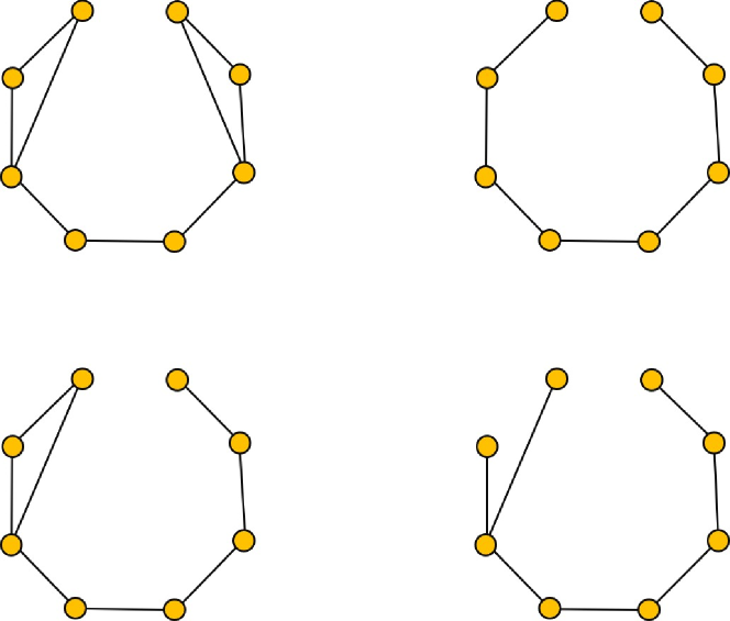
The four graphs with the largest value of $\mathcal{\mathcal{\mathscr{R}}_{\mathnormal{\alpha=1}}}\left(G\right)$ among all connected graphs with 8 vertices are illustrated in Fig. 4.1.

Figure 4.1: Graphs with the maximum values of $\mathcal{\mathcal{\mathscr{R}}_{\mathnormal{\alpha=1}}}\left(G\right)$ among all connected graphs with 8 vertices.

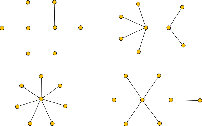
Lemma 4.11.

Let $\alpha\in\{-1,1\}$. Then

$$\mathcal{\mathcal{\mathscr{R}}_{\mathnormal{\alpha=-1}}}\left(G\right){\color[rgb]{0,0,0}{{\color[rgb]{0,0,0}\geq\dfrac{n\left(n-1\right)}{2\varDelta}}}.}$$ (4.24)

Proof.

Again by Remark 3.13, $\rho_{\alpha=-1,n}\leq 2\varDelta$. Then, $\underset{i}{\max}c_{\alpha=-1}\left(i\right)=\underset{i}{\max}k_{i}^{-1}\sum_{v\in\eta_{i}}k_{v}$, with the maximum being attained at those vertices $i$ with minimal degree $k_{i}=\delta$ and connected to $\delta$ vertices $v\in\eta_{i}$ which all have the maximum degree $\varDelta$. Thus, the result follows using the Corollary 4.7. ∎

The four graphs with the largest value of $\mathcal{\mathcal{\mathscr{R}}_{\mathnormal{\alpha=-1}}}\left(G\right)$ among all connected graphs with 8 vertices are illustrated in Fig. 4.2.

Figure 4.2: Graphs with the maximum values of $\mathcal{\mathcal{\mathscr{R}}_{\mathnormal{\alpha=-1}}}\left(G\right)$ among all connected graphs with 8 vertices.

Remark 4.12.

In $d$-regular graphs, $c_{\alpha=1}\left(v,w\right)=c_{\alpha=-1}\left(v,w\right)=1$ for all $\left(v,w\right)\in E$. Thus, $\Omega_{\alpha=1}\left(v,w\right)=\Omega_{\alpha=-1}\left(v,w\right)=\Omega\left(v,w\right)$ for all $\left(v,w\right)\in E$, and $\mathcal{\mathcal{\mathscr{R}}_{\mathnormal{\alpha=1}}}\left(G\right)=\mathcal{\mathcal{\mathscr{R}}_{\mathnormal{\alpha=-1}}}\left(G\right)=\mathcal{\mathcal{\mathscr{R}}}_{\alpha=0}$.

Then, we calculated the hubs-repelling $\mathcal{\mathcal{\mathscr{R}}_{\mathnormal{\alpha=1}}}\left(G\right)$, attracting $\mathcal{\mathcal{\mathscr{R}}_{\mathnormal{\alpha=-1}}}\left(G\right)$ and normal $\mathcal{\mathcal{\mathscr{R}}}_{\alpha=0}\left(G\right)$ Kirchhoff indices for all connected graphs with $5\leq n\leq 8$. In general, we observed for these more than 12,000 graphs that: $\mathcal{\mathcal{\mathscr{R}}_{\mathnormal{\alpha=1}}}\left(G\right)\geq\mathcal{\mathcal{\mathscr{R}}}_{\alpha=0}\left(G\right)\geq\mathcal{\mathcal{\mathscr{R}}_{\mathnormal{\alpha=-1}}}\left(G\right)$. Finally we formulate the following conjecture for the Kirchhoff indices of graphs.

Conjecture 4.13.

Let $\alpha\in\{-1,1\}$. Then

$$\mathcal{\mathcal{\mathscr{R}}_{\mathnormal{\alpha=1}}}\left(G\right)\geq\mathcal{\mathcal{\mathscr{R}}}_{\alpha=0}\left(G\right)\geq\mathcal{\mathcal{\mathscr{R}}_{\mathnormal{\alpha=-1}}}\left(G\right),$$ (4.25)

with equality if and only if $G$ is regular.

5 Computational results

5.1 Random-walks connection

Let us consider a “particle” performing a standard random walk through the vertices and edges of any of the networks studied here. The use of random walks in graphs [35] and networks [36] is one of the most fundamental types of stochastic processes, used to model diffusive processes, different kinds of interactions, and opinions among humans and animals [36]. They can also be used as a way to extract information about the structure of networks, including the detection of dense groups of entities in a network [36]. Then, we consider a random walk on $G$, which represents the real-world network under consideration. We start at a vertex $v_{0}$; if at the $r$th step we are at a vertex $v_{r}$, we move to any neighbor of $v_{r}$, with probability $k_{r}^{-1},$ where $k_{r}$ is the degree of the vertex $r$. Clearly, the sequence of random vertices ($v_{t}:t=0,1,\ldots$) is a Markov chain [35].

An important quantity in the study of random walks on graphs is the access or hitting time $\mathcal{H}\left(v,w\right),$ which is the number of steps before vertex $w$ is visited, starting from vertex $v$ [35]. The sum $\mathcal{C}\left(v,w\right)=\mathcal{H}\left(v,w\right)+\mathcal{H}\left(w,v\right)$ is called the commute time, which is the number of steps in a random walk starting at $v$, before vertex $w$ is visited and then the walker comes back again to vertex $v$ [35]. The connection between random walks and resistance distance on graphs is then provided by the following result (see for instance [1]), where we as usual denote by $c\left(v\right)$ the vertex conductances of vertices $v$.

Lemma 5.1.

For any two vertices $v$ and $w$ in $G$, the commute time is

$$\mathcal{C}\left(v,w\right)=\textnormal{vol}(G)\Omega\left(v,w\right).$$ (5.1)

Here and in the following, $\textnormal{vol}(G)=\sum\limits_{v=1}^{n}c\left(v\right)$ is volume of the graph. (Notice that if the graph is unweighted (the case formally corresponding to $\alpha=0$) then by the Handshaking Lemma $\textnormal{vol}(G)=2m$.) The “efficiency” of a standard random walk process on $G$ can then be measured by

$$\varepsilon\left(G\right)=1/\sum_{v,w}{\mathcal{C}}\left(v,w\right),$$ (5.2)

That is, if a standard random walker on a graph uses small times to commute between every pair of vertices in the graph, it is an efficient navigational process. On the contrary, large commuting times between pairs of vertices reveal very inefficient processes. Obviously, $\varepsilon\left(G\right)=1/\left(\textnormal{vol}(G)\sum_{v,w}\Omega\left(v,w\right)\right)$.

We now extend these concepts to the use of hubs-biased random walks and calculated the Kirchhoff indices $\mathcal{\mathcal{\mathscr{R}}}\left(G\right),$ $\mathcal{\mathcal{\mathscr{R}}_{\mathnormal{\alpha=-1}}}\left(G\right)$ and $\mathcal{\mathcal{\mathscr{R}}_{\mathnormal{\alpha=1}}}\left(G\right)$ for all these networks. Following a similar reasoning as before we define the efficiencies of the hubs-biased random walks by:

$$\varepsilon_{\alpha}\left(G\right)\coloneqq 1/\left(\textnormal{vol}_{\alpha}\sum_{v,w}{\Omega}_{\alpha}\left(v,w\right)\right),$$ (5.3)

where $\textnormal{vol}_{\alpha}$ is the volume of the graph with conductances based on $\alpha$. We are interested here in the efficiency of the hubs-biased random walk processes relative to the standard random walk. We propose to measure these relative efficiencies by

$$\mathscr{E}_{\alpha}\left(G\right)\coloneqq\dfrac{\varepsilon_{\alpha}\left(G\right)}{\varepsilon\left(G\right)}=\dfrac{\textnormal{vol}}{\textnormal{vol}_{\alpha}}\dfrac{\mathcal{\mathcal{\mathscr{R}}}\left(G\right)}{\mathcal{\mathcal{\mathscr{R}}_{\mathnormal{\alpha}}}\left(G\right)}.$$ (5.4)

When $\mathscr{E}_{\alpha}\left(G\right)>1$ the hubs-biased random walk is more efficient than the standard random walk. On the other hand, when $\mathscr{E}_{\alpha}\left(G\right)<1$ the standard random walk is more efficient than the hubs-biased one. When the efficiency of both processes, hubs-biased and standard, are similar we have $\mathscr{E}_{\alpha}\left(G\right)\approx 1$.

5.2 Efficiency in small graphs

We start by analyzing the 11,117 connected graphs with 8 vertices that we studied previously. In Fig. 5.1 we illustrate the results in a graphical way. As can be seen

• $\mathscr{E}_{\alpha=-1}\left(G\right)>1$ for 95.7% of the graphs considered (10,640 out of 11,117), indicating that in the majority of graphs a hubs-attracting random walk can be more efficient than the standard random walk driven by the unweighted Laplacian, corresponding to $\alpha=0$;

• $\mathscr{E}_{\alpha=1}\left(G\right)>1$ only in 91 out of the 11,117 graphs, which indicates that hubs-repelling random walks are more efficient than the standard random walk only for very few graphs;

• All graphs for which $\mathscr{E}_{\alpha=1}\left(G\right)\geq 1$ also have $\mathscr{E}_{\alpha=-1}\left(G\right)\geq 1$, with equality only for regular graphs;

• Only 461 graphs (4.15% of all graphs considered) have simultaneously $\mathscr{E}_{\alpha=1}\left(G\right)<1$ and $\mathscr{E}_{\alpha=-1}\left(G\right)<1$. These are graphs for which the standard random walk is more efficient than both hubs-biased random walks;

• Only 17 graphs have $\mathscr{E}_{\alpha=1}\left(G\right)=\mathscr{E}_{\alpha=-1}\left(G\right)=1$. They are all the regular graphs having 8 nodes that exist.

Figure 5.1: Plot of the efficiency of hubs-biased random walks relative to the standard one for all 11,117 connected graphs with 8 vertices.

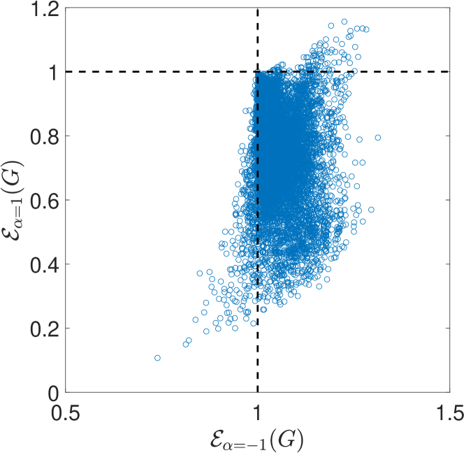
These results bring some interesting hints about the structural characteristics that the graphs have to display to be benefited from hubs-biased processes. For instance, the fact that most of the graphs can be benefited from hubs-attracting ($\alpha=-1$) random walks is explained as follow. A standard random walk typically does not follow the shortest topological path connecting a pair of non-connected vertices. However, the number of shortest paths crossing a vertex increases with the degree of that vertex. For instance, let $k_{v}$ and $t_{v}$ be the degree and the number of triangles incident to a vertex $v$. The number of shortest paths connecting pairs of vertices is $P\geq\dfrac{1}{2}k_{v}\left(k_{v}-1\right)-t_{v}$. Therefore, the hubs-attracting strategy induces the random walker to navigate the network using many of the shortest paths interconnecting pairs of vertices, which obviously decreases the commute time and increases the efficiency of the process. Most networks can be benefited from this strategy.

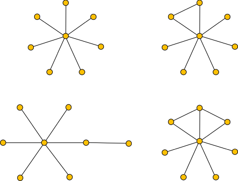
The case of the hubs-repelling strategies is more subtle. To reveal the details we illustrate the four graphs having the minimum efficiency of a hubs-repelling ($\alpha=1$) random walk in Fig. 5.2. As can be seen all these graphs have star-like structures, which are the graphs with the largest possible degree heterogeneity [20, 21]. Therefore, in these graphs the use of hubs-repelling strategies lets the random walker get trapped in small degree vertices without the possibility of visiting other vertices, because for such navigation they have to cross the hubs of the graph, a process which is impeded by the hubs-repelling strategy.

Figure 5.2: Illustration of the graphs with the minimum values of $\mathscr{E}_{\alpha=1}\left(G\right)$ among the 11,117 connected graphs with 8 vertices.

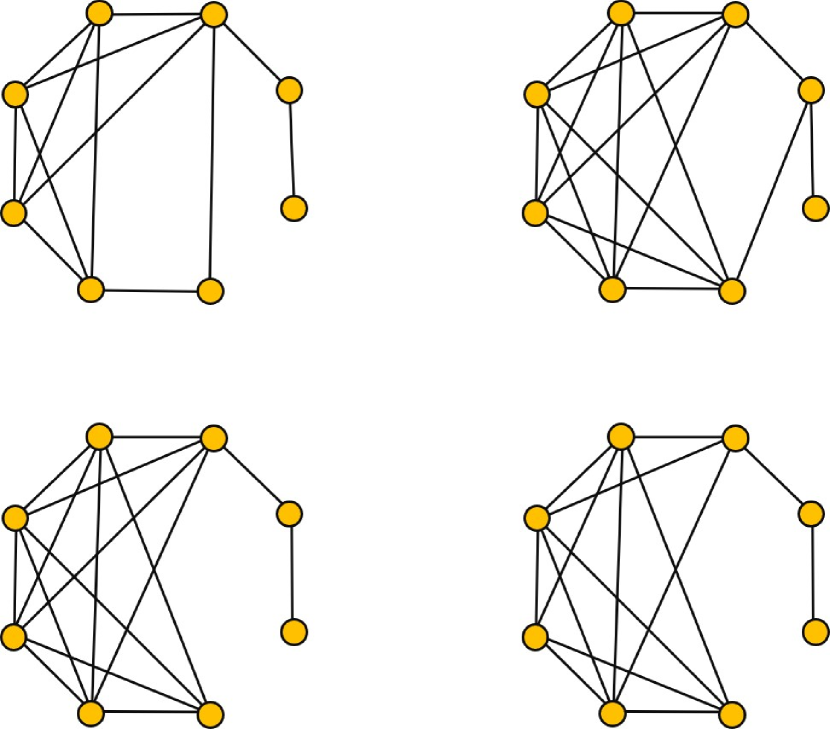
The previous analysis allows us to consider the reason why so little number of graphs display $\mathscr{E}_{\alpha=1}\left(G\right)>1$. Such graphs have to display very small degree heterogeneity, but without being regular, as for regular graphs $\mathscr{E}_{\alpha=1}\left(G\right)=1$. The four graphs with the highest value of $\mathscr{E}_{\alpha=1}\left(G\right)$ among all connected graphs with 8 vertices are illustrated in Fig. 5.3. As can be seen these graphs display “quasi-regular” structures but having at least one pendant vertex connected to another low-degree vertex. Then, in a hubs-repelling strategy this relatively isolated vertex (the pendant one) has larger changes (than in a standard random walk) of being visited by the random walker who is escaping from the vertices of larger degree.

Figure 5.3: Illustration of the graphs with the maximum values of $\mathscr{E}_{\alpha=1}\left(G\right)$ among the 11,117 connected graphs with 8 vertices.

In closing, we have observed that hubs-attracting random walks are very efficient in most of graphs due to the fact that such processes increase the chances of navigating the graph through their shortest paths. On the other hand, hubs-repelling random walks are efficient only in those quasi-regular graphs having some relatively isolated vertices which can be visited by the hubs-repelling walker with higher chances than in a standard random walk.

5.3 Efficiency in real-world networks

Here we study 59 real-world networks representing brain/neuronal systems, electronic circuits, social systems, food webs, protein-protein interaction networks (PIN), modular software, citation networks, transcription networks and infrastructure networks. The description of all the networks is in the Appendix of the book [19].

The results obtained here for the 59 real-world networks are resumed in Table 1 where we report the average values of the previous indices for groups of networks in different functional classes, i.e., brain networks, electronic circuits, social networks, etc.

type	number	$\mathscr{\bar{E}}_{\alpha=1}\left(G\right)$	std	$\mathscr{\bar{E}}_{\alpha=-1}\left(G\right)$	std
brain	3	0.6365	0.2552	0.9938	0.0489
circuits	3	0.5187	0.0277	1.0662	0.0095
foodweb	14	0.4134	0.2715	1.1247	0.2545
social	12	0.3536	0.1917	1.0103	0.1812
citations	7	0.2032	0.1758	0.8199	0.2769
PIN	8	0.1385	0.0896	0.7855	0.1864
infrastructure	4	0.0869	0.1439	0.4846	0.4638
software	5	0.0712	0.0296	0.6148	0.1515
transcription	3	0.0711	0.0710	0.5806	0.3218

Table 1: Average values of the relative efficiency of using a hubs-attracting random walk on the graph with respect to the use of the standard random walk: $\mathscr{\bar{E}}_{\alpha=-1}\left(G\right)$ for different networks grouped in different classes. The number of networks in each class is given in the column labeled as “number”. The same for a hubs-repelling random walk: $\mathscr{\bar{E}}_{\alpha=1}\left(G\right)$. In both cases the standard deviations of the samples of networks in each class is also reported.

The main observations from the analysis of these real-world networks are:

• $\mathscr{E}_{\alpha=-1}\left(G\right)>1$ for 50.8% of the networks considered, indicating that only in half of the networks a hubs-attracting random walk can be more efficient than the standard random walk;

• $\mathscr{E}_{\alpha=1}\left(G\right)>1$ in none of the networks, which indicates that standard random walks are always more efficient than hubs-repelling random walks in all these networks.

The first result is understood by the large variability in the degree heterogeneity of real-world networks. In this case, only those networks with skew degree distributions are benefited from the use of hubs-attracting random walks, while in those with more regular structures are not.

The second result indicates that there are no network with such quasi-regular structures where some of the vertices are relatively isolated as the graphs displayed in Fig. 5.3. However, as usual the devil is in the details. The analysis of the results in Table 1 indicates that brain networks, followed closely by electronic flip-flop circuits, are the networks in which the use of hubs-repelling strategies of navigation produces the highest efficiency relative to standard random walks. This can also be read as that these brain networks have evolved in a way in which their topologies guarantee random walk processes as efficient as the hubs-attracting ones without the necessity of navigating the brain using such specific mechanisms. In addition, the use of hubs-repelling processes do not affect significantly the average efficiency of brain networks, as indicated by the value of $\mathscr{\bar{E}}_{\alpha=1}\left(G\right),$ which is very close to one. This result indicates that if these networks have to use a hubs-repelling strategies of navigation due to certain biological constraints, they have topologies which are minimally affected – in terms of efficiency – when using such strategies.

Finally, another remarkable result is that the efficiency of navigational processes in infrastructural and modular software systems is more than 1000% efficient by using normal random-walk approaches than by using hubs-repelling strategies. Those infrastructural networks seem to be wired to be navigated by using their hubs, and avoiding them cost a lot in terms of efficiency. This is clearly observed in many transportation networks, such as air transportation networks, where the connection between pairs of airports is realized through the intermediate of a major airport, i.e., a hub, in the network.

6 Conclusions

We have introduced the concept of hubs-biased resistance distance. These Euclidean distances are based on graph Laplacians which consider the edges $e=\left(v,w\right)$ of a graph weighted by the degrees of the vertices $v$ and $w$ in a double orientation of that edge. Therefore, the hubs-biased Laplacian matrices are non-symmetric and reflect the capacity of a graph/network to diffuse particles using hubs-attractive or hubs-repulsive strategies. The corresponding hubs-biased resistance distances and the corresponding Kirchhoff indices can be seen as the efficiencies of these hubs-attracting/repelling random walks of graphs/networks. We have proved several mathematical results for both the hubs-biased Laplacian matrices and the corresponding resistances and Kirchhoff indices. Finally we studied a large number of real-world networks representing a variety of complex systems in nature, and society. All in all we have seen that there are networks which have evolved, or have being designed, to operate efficiently under hubs-attracting strategies. Other networks, like brain ones, are almost immune to the change of strategies, because the use of hubs-attracting strategies improve very little the efficiency of a standard random walk, and the efficiency of hubs-repelling strategies is not significantly different than that of the classical random walks. Therefore, in such networks the use of the standard random walk approach is an efficient strategy of navigation, while infrastructures and modular software networks seem to be designed to be navigated by using their hubs.

References

- [1] D. Aldous, and J. Fill, Reversible Markov Chains And Random Walks On Graphs. Book in preparation. Available at: https://www.stat.berkeley.edu/~aldous/RWG/book.pdf.
- [2] A. Ali, I. Gutman, E. Milovanović, and I. Milovanović, Sum of Powers of the Degrees of Graphs: Extremal Results and Bounds, MATCH Commun. Math. Comput. Chem. 80 (2018), 5–84.
- [3] M. Bianchi, J.L. Palacios, A. Torriero, and A.L. Wirkierman, Kirchhoffian indices for weighted digraphs. Discrete Applied Mathematics 255 (2019) 142–154.
- [4] S. Boccaletti, V. Latora, Y. Moreno, M. Chavez, and D.-U. Hwang, Complex networks: Structure and dynamics, Phys. Rep. 424 (2006), 175–308.
- [5] D. Boley, G. Ranjan, and Z. L. Zhang, Commute times for a directed graph using an asymmetric Laplacian. Lin. Algebra Appl. 435 (2011), 224–242.
- [6] M. Bonaventura, V. Nicosia, and V. Latora, Characteristic times of biased random walks on complex networks. Phys. Rev. E. 89 (2014), 012803.
- [7] Z.M. Boyd, N. Fraiman, J. Marzuola, P.J. Mucha, B. Osting, and J. Weare, A metric on directed graphs and Markov chains based on hitting probabilities. SIAM J. Math. Data Science 3 (2021), 467–493.
- [8] A. Bunde, J. Caro, J. Kärger, and G. Vogl (eds.), Diffusive Spreading in Nature, Technology and Society, Springer-Verlag, Berlin, 2017.
- [9] Z. Burda, J. Duda, J. M. Luck, and B. Waclaw, Localization of the maximum entropy random walk. Phys. Rev. Lett. 102 (2009), 160602.
- [10] F. R. K. Chung, Spectral Graph Theory. Vol. 92 of Reg. Conf. Series Math., Amer. Math. Soc., Providence (RI), 1997.
- [11] S. M. Cioabă, Sums of powers of the degrees of a graph. Discrete Math. 306 (2006), 1959–1964.
- [12] D. Coppersmith, U. Feige, and J. Shearer, Random walks on regular and irregular graphs. SIAM J. Discr. Math. 9 (1996), 301–308.
- [13] K. C. Das, Maximizing the sum of the squares of the degrees of a graph. Discrete Math. 285 (2004), 57–66.
- [14] K. C. Das, On the Kirchhoff index of graphs. Zeitsch. Naturforsch. A. 68 (2013), 531–538.
- [15] K. C. Das, K. Xu, and J. Nam, Zagreb indices of graphs. Front. Math. China 10 (2015), 567–582.
- [16] N. M. De Abreu, Old and new results on algebraic connectivity of graphs. Lin. Algebra Appl. 423 (2007), 53–73.
- [17] P. G. Doyle and J. L. Snell, Random Walks And Electric Networks. vol. 22 of Carus Math. Monogr., Math. Assoc. Amer., Washington (DC), 1984.
- [18] W. Ellens, F. M. Spieksma, P. Van Mieghem, A. Jamakovic, and R. E. Kooij, Effective graph resistance. Lin. Algebra Appl. 435 (2011), 2491–2506.
- [19] E. Estrada, The Structure Of Complex Networks: Theory And Applications, Oxford University Press, Oxford, 2012.
- [20] E. Estrada, Degree heterogeneity of graphs and networks. I. Interpretation and the “heterogeneity paradox”. J. Interdisc. Math. 22 (2019), 503–529.
- [21] E. Estrada, Degree heterogeneity of graphs and networks. II. Comparison with other indices. J. Interdisc. Math. 22 (2019), 711–735.
- [22] E. Estrada, ‘Hubs-repelling’ Laplacian and related diffusion on graphs/networks. Lin. Algebra Appl. 596 (2020), 256–280.
- [23] M. Fiedler, Algebraic connectivity of graphs, Czechoslovak Math. J. 23 (1973), 298–305.
- [24] M. Fiedler, Laplacian of graphs and algebraic connectivity, Banach Center Publications 25 (1989), 57–70.
- [25] K. Fitch, Effective resistance preserving directed graph symmetrization. SIAM J. Matrix Analysis Appl. 40 (2019), 49–65.
- [26] L. V. Gambuzza, M. Frasca, and E. Estrada, Hubs-attracting Laplacian and Related Synchronization on Networks. SIAM J. Appl. Dyn. Syst. 19 (2020), 1057–1079.
- [27] A. Gerbaud, K. Altisen, S. Devismes, and P. Lafourcade, Comparison of mean hitting times for a degree-biased random walk. Discr. Appl. Math. 19 (2014), 104–109.
- [28] A. Ghosh, S. Boyd, and A. Saberi, Minimizing effective resistance of a graph. SIAM Rev. 50 (2008), 37–66.
- [29] R. Grone, R. Merris, and V. S. Sunder, The Laplacian spectrum of a graph, SIAM J. Matrix Anal. Appl. 11 (1990), 218–238.
- [30] R. Grone and R. Merris, The Laplacian spectrum of a graph II, SIAM J. Matrix Anal. Appl. 7 (1994), 221–229.
- [31] I. Gutman, L. Feng, and G. Yu, Degree resistance distance of unicyclic graphs. Trans. Combinat. 1 (2012), 27–40.
- [32] P.T. Harker, Alternative modes of questioning in the analytic hierarchy process. Mathematical Modelling 9 (1987), 353–360.
- [33] J. B. Kennedy, P. Kurasov, G. Malenová, and D. Mugnolo, On the spectral gap of a quantum graph. Ann. Henri Poincaré 17 (2016), 2439–2473.
- [34] D. J. Klein, and M.Randić, Resistance distance. J. Math. Chem. 12 (1993), 81–95.
- [35] L. Lovász, Random walks on graphs: A survey. In: D. Miklos, V. T. Sos, and T. Szonyi (eds.), Combinatorics, Paul Erdős is Eighty, Vol. 2, János Bolyai Mathematical Society, Budapest, 1993, pp. 1–46.
- [36] N. Masuda, M. A. Porter, and R. Lambiotte, Random walks and diffusion on networks. Phys. Rep. 716 (2017), 1–58.
- [37] R. Merris, Laplacian matrices of graphs: a survey. Lin. Algebra Appl. 197 (1994), 143–176.
- [38] B. Mohar, The Laplacian spectrum of graphs. In: Y. Alavi, G. Chartrand, O. R. Oellermann, and A. J. Schwenk (eds.), Graph Theory, Combinatorics, and Applications, Vol. 2, Wiley, New York, 1991, pp. 871–898.
- [39] R. J. Mondragón, Core-biased random walks in networks. J. Complex Net. 6 (2018), 877–886.
- [40] D. Mugnolo, Semigroup Methods For Evolution Equations On Networks. Springer-Verlag, Cham, 2014.
- [41] M. E. Newman. Spread of epidemic disease on networks. Phys. Rev. E 66 (2002), 016128.
- [42] M. E. Newman, The structure and function of complex networks, SIAM Review 45 (2003), 167–256.
- [43] J. L. Palacios, Resistance distance in graphs and random walks. Int. J. Quantum Chem. 81 (2001), 29–33.
- [44] J. L. Palacios, Closed-form formulas for Kirchhoff index. Int. J. Quantum Chem. 81 (2001), 135–140.
- [45] C. Poignard, T. Pereira, and J. P. Pade, Spectra of Laplacian matrices of weighted graphs: structural genericity properties, SIAM J. Appl. Math. 78 (2018), 372–394.
- [46] C. Seguin, M. P. Van Den Heuvel, and A. Zalesky, Navigation of brain networks. Proc. Natl. Acad. Sci. USA 115 (2018), 6297–6302.
- [47] D. Tomasi, G. J. Wang, and N. D. Volkow, Energetic cost of brain functional connectivity. Proc. Natl. Acad. Sci. USA 110 (2013), 13642–13647.
- [48] W. Xiao, and I. Gutman, Resistance distance and Laplacian spectrum. Theoret. Chem. Acc. 110 (2003), 284–289.
- [49] G. F. Young, L. Scardovi, and N. E. Leonard, A new notion of effective resistance for directed graphs – Part I: Definition and properties. IEEE Transactions on Automatic Control. 61 (2015), 1727–1736.
- [50] B. Zhou, and N. Trinajstić. On resistance-distance and Kirchhoff index. J. Math. Chem. 46 (2009), 283–289.